histogram-based prefiltering for luminance and chrominance
TRANSCRIPT

IEEE Transaction on Circuits and Systems for Video Technology
Vol. 18, No. 9, 2008
Ulrich Fecker, Marcus Barkowsky, and Andre Kaup
Presented by Euiwon Nam
School of Electrical Engineering and Computer Science
Kyungpook National Univ.
Histogram-based Prefiltering for
Luminance and Chrominance
Compensation of Multiview Video
Abstract
Histogram-based prefiltering
– Luminance and chrominance compensation
• Time-constant calculation of mapping function
− Adoption cumulative histogram
» Distorted sequence to reference sequence
• RGB color conversion
• Use of global disparity compensation
− Combination with JMVM S/W
» Block-based illumination compensation
2/26

Introduction
Multiview video
– Technique for recording object or scene
• Static light fields
− Rigid and nonmoving objects
• Dynamic light fields
− Moving objects or scenes
Application for multiview video
– Three-dimensional television
– Free-veiwpoint television
– 3-D visualizations of inner organs of human
• Image-based rendering technique for medicine
3/26

Recoding of multiview video
– Simulcast coding
• Using H.264/AVC video coding standard independently
• Improvement of efficiency
− Using both temporal correlation and spatial correlation
• Motion compensation and disparity compensation
− Using reference
• Current scheme
− Joint Video Team of ISO/IEC MPEG and ITU-T VCEG
4/26
luminance and chrominance variations
– Impairing performance of multiview coder or renderer
• Block-based illumination compensation for Joint Video Team
− Improvement coding efficiency in H264/AVC
» By predictive coding of DC coefficient of integer transform
• Histogram matching as proposed method
− Fitting distorted image to reference image
» Adapting cumulative histogram of distorted image to reference
5/26
Proposed method
– Histogram matching
• Adapting all camera views to reference view
• Advantage for processing
− Non-assumption type of distortion like brightness or contrast variation
− Non-consideration of nonlinear operations
− Useful to correct global discrepancies in luminance and chrominance
» Applying to entire image for correction
− Preserving local illumination change
6/26
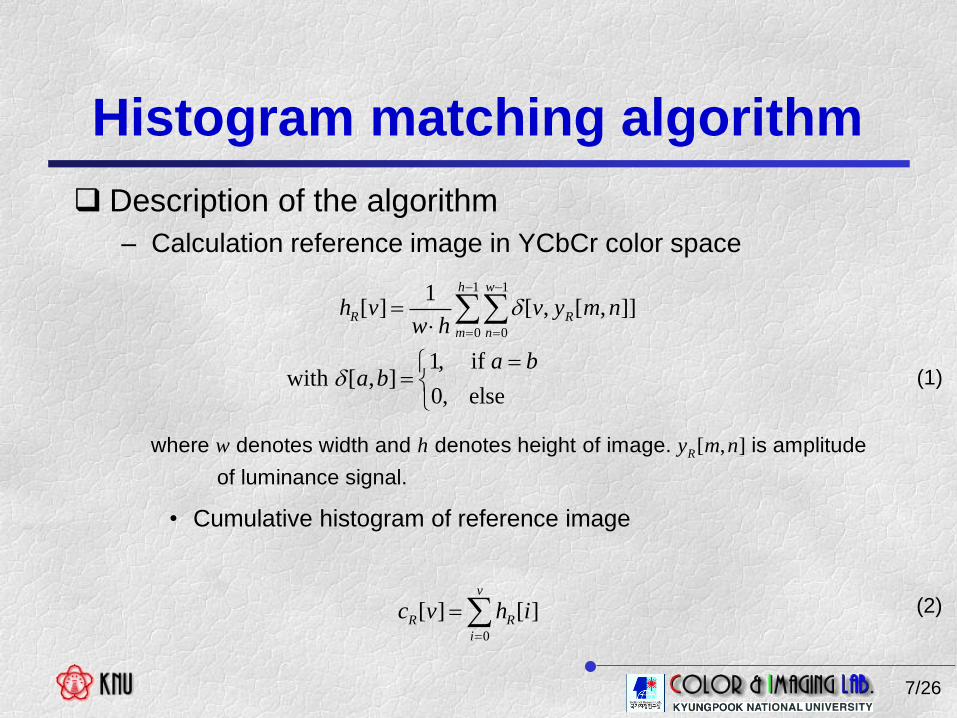
Histogram matching algorithm
Description of the algorithm
– Calculation reference image in YCbCr color space
• Cumulative histogram of reference image
1 1
0 0
1 [ ] [ , [ , ]]
1, if with [ , ]
0, else
h w
R R
m n
h v v y m nw h
a ba b
(1)
[ , ]Rw h y m nwhere denotes width and denotes height of image. is amplitude
of luminance signal.
0
[ ] [ ]v
R R
i
c v h i
(2)
7/26
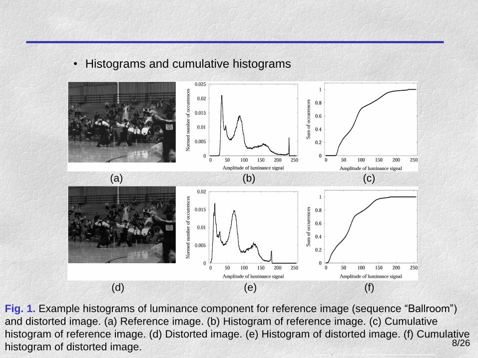
• Histograms and cumulative histograms
(a) (b) (c)
(d) (e) (f)
Fig. 1. Example histograms of luminance component for reference image (sequence “Ballroom”)
and distorted image. (a) Reference image. (b) Histogram of reference image. (c) Cumulative
histogram of reference image. (d) Distorted image. (e) Histogram of distorted image. (f) Cumulative
histogram of distorted image. 8/26

– Mapping function based on cumulative histograms
• Applying mapping to distorted image
[ ] with [ ] [ ] [ 1]R D RM v u c u c v c u (3)
Fig. 2. Details of mapping algorithm shown in section of cumulative histogram.
[ , ] [ [ , ]]C Dy m n M y m n (4)
9/26
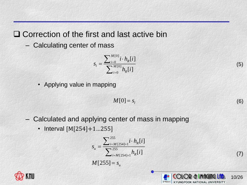
Correction of the first and last active bin
– Calculating center of mass
• Applying value in mapping
– Calculated and applying center of mass in mapping
• Interval [M[254]+1…255]
[0]
0
[0]
0
[ ]
[ ]
M
Ril M
Ri
i h is
h i
(5)
[0] lM s (6)
255
[254] 1
255
[254] 1
[ ]
[ ]
[255]
Ri M
u
Ri M
u
i h is
h i
M s
(7)
10/26

Application to multiview sequence
– Correcting all other camera fitting histogram
• Using histogram of chosen reference view
Fig. 3. Example for histogram of corrected image compared with the reference image and distorted
image (sequence “Ballroom”). 11/26

Effect of histogram matching on multiview coding
Statistical evaluation of the prediction step
– Using Minimum mean square error(MSE)
12/26 Fig. 4. Prediction scheme assumed for the statistical analysis.
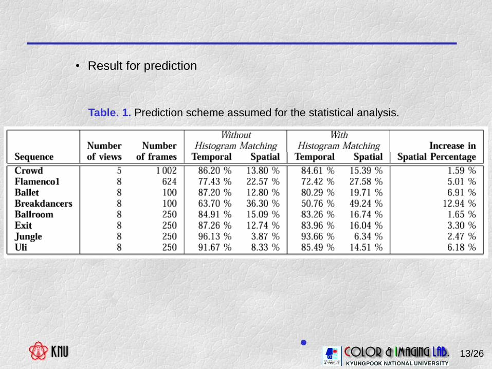
• Result for prediction
13/26
Table. 1. Prediction scheme assumed for the statistical analysis.

Effect on the JMVM multiview video coder
– Compared coding performance with and without histogram matching
Fig. 5. Coding performance using the basic histogram matching algorithm(“Ballroom”, eight views).
Average PSNR difference: -0.26 dB (Y), 0.00 dB(Cb), and -0.28 dB (Cr). 14/26

Extensions to the algorithm
Time-constant mapping function
– Compensation of deteriorated coding performance
• Extension mapping function by modifying Eq.(1)
1 1 1
0 0 0
1 [ ] [ , [ , , ]]
1, if with [ , ]
0, else
l h w
R R
t m n
h v v y m n tl w h
a ba b
(8)
[ , , ]
.
Ry m n t t
l
where denotes amplitude of luminance image at time step of
reference view. Length of sequence is denoted by
15/26

• Coding performance by extension mapping function
Fig. 6. Coding performance using time-constant histogram matching (“Ballroom,” eight views).
Average PSNR difference: 0.05 dB (Y), 0.15 dB (Cb), and -0.02 dB (Cr).
16/26
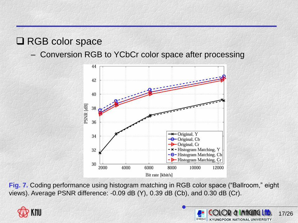
RGB color space
– Conversion RGB to YCbCr color space after processing
Fig. 7. Coding performance using histogram matching in RGB color space (“Ballroom,” eight
views). Average PSNR difference: -0.09 dB (Y), 0.39 dB (Cb), and 0.30 dB (Cr).
17/26
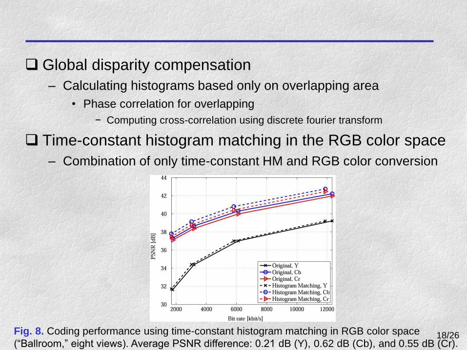
Global disparity compensation
– Calculating histograms based only on overlapping area
• Phase correlation for overlapping
− Computing cross-correlation using discrete fourier transform
Time-constant histogram matching in the RGB color space
– Combination of only time-constant HM and RGB color conversion
Fig. 8. Coding performance using time-constant histogram matching in RGB color space
(“Ballroom,” eight views). Average PSNR difference: 0.21 dB (Y), 0.62 dB (Cb), and 0.55 dB (Cr). 18/26

– Block diagram for processing
Fig. 9. Block diagram of proposed algorithm. Time-constant histogram matching is applied in RGB
color space before color conversion, chrominance downsampling, and multiview coding.
19/26

Reversibility of the algorithm
– Applying inverse of mapping function
Fig. 10. Example for mapping function in RGB color space and its inverse (Race1, view 0, R
component).
20/26
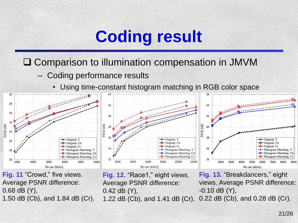
Coding result
Comparison to illumination compensation in JMVM
– Coding performance results
• Using time-constant histogram matching in RGB color space
Fig. 11 “Crowd,” five views.
Average PSNR difference:
0.68 dB (Y),
1.50 dB (Cb), and 1.84 dB (Cr).
Fig. 12. “Race1,” eight views.
Average PSNR difference:
0.42 dB (Y),
1.22 dB (Cb), and 1.41 dB (Cr).
Fig. 13. “Breakdancers,” eight
views. Average PSNR difference:
-0:10 dB (Y),
0.22 dB (Cb), and 0.28 dB (Cr).
21/26
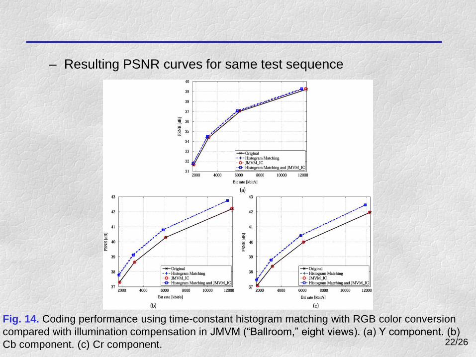
– Resulting PSNR curves for same test sequence
Fig. 14. Coding performance using time-constant histogram matching with RGB color conversion
compared with illumination compensation in JMVM (“Ballroom,” eight views). (a) Y component. (b)
Cb component. (c) Cr component. 22/26

– Other sequence
Fig. 15. Coding performance using time-constant histogram matching with RGB color conversion
compared to illumination compensation in JMVM (“Crowd”, 5 views). (a) Y component, (b) Cb
component, (c) Cr component. 23/26

– Other sequence
Fig. 16. Coding performance using time-constant histogram matching with RGB color conversion
compared to illumination compensation in JMVM (“Race1”, 8 views). (a) Y component, (b) Cb
component, (c) Cr component. 24/26

– Resulting PSNR curves
Fig. 17. Coding performance using time-constant histogram matching with RGB color conversion
compared to illumination compensation in JMVM (“Breakdancers”, 8 views). (a) Y component, (b) Cb
component, (c) Cr component. 25/26

– Average PSNR gains
Table. 2. Average PSNR gains of histogram matching, JMVM-IC as well as combination of histogram
matching and JMVM-IC. PSNR differences are always calculated compared to multiview coding
without luminance or chrominance compensation
26/26

Summary and conclusion
Histogram matching
– Compensation of luminance and chrominance components
• Extended as time-constant histogram matching
– Combination with Illumination compensation method
• Implementation prefiltering in JMVM software
– Result of coding performance
• Improvement of performance for compensating
27/26