hille and nehari type criteria for third-order dynamic ...apeterson1/pub/thirdhillenehari.pdf ·...
TRANSCRIPT

HILLE AND NEHARI TYPE CRITERIA FORTHIRD-ORDER DYNAMIC EQUATIONS
L. ERBE, A. PETERSON AND S. H. SAKER
Abstract. In this paper, we extend the oscillation criteria that havebeen established by Hille [15] and Nehari [21] for second-order differentialequations to third order dynamic equations on an arbitrary time scaleT, which is unbounded above. Our results are essentially new even forthird order differential and difference equations, i.e. when T = R andT = N. We consider several examples to illustrate our results.
Keywords and Phrases: Oscillation, third-order dynamic equa-tions, time scales.
2000 AMS Subject Classification: 34K11, 39A10, 39A99.
1. Introduction
The study of dynamic equations on time scales, which goes back to itsfounder Stefan Hilger [14], is an area of mathematics that has recently re-ceived a lot of attention. It has been created in order to unify the studyof differential and difference equations. Many results concerning differen-tial equations carry over quite easily to corresponding results for differenceequations, while other results seem to be completely different from theircontinuous counterparts. The study of dynamic equations on time scalesreveals such discrepancies, and helps avoid proving results twice - once fordifferential equations and once again for difference equations. The generalidea is to prove a result for a dynamic equation where the domain of theunknown function is a so-called time scale T, which is a nonempty closedsubset of the reals R. In this way results not only related to the set of realnumbers or set of integers but those pertaining to more general time scalesare obtained.
The three most popular examples of calculus on time scales are differen-tial calculus, difference calculus (see [17]), and quantum calculus (see Kacand Cheung [16]), i.e, when T = R, T = N and T = qN0 = {qt : t ∈ N0},where q > 1. Dynamic equations on a time scale have an enormous poten-tial for applications such as in population dynamics. For example, it can
1991 Mathematics Subject Classification. 34K11, 39A10, 39A99.Key words and phrases. Oscillation, third-order dynamic equations, time scales.
1

2 L. ERBE, A. PETERSON AND S. H. SAKER
model insect populations that are continuous while in season, die out insay winter, while their eggs are incubating or dormant, and then hatch in anew season, giving rise to a nonoverlapping population (see [4]). There areapplications of dynamic equations on time scales to quantum mechanics,electrical engineering, neural networks, heat transfer, and combinatorics. Arecent cover story article in New Scientist [29] discusses several possible ap-plications. The books on the subject of time scales by Bohner and Peterson[4] and [5] summarize and organize much of time scale calculus and someapplications.
For completeness, we recall the following concepts related to the notionof time scales. A time scale T is an arbitrary nonempty closed subset ofthe real numbers R. We assume throughout that T has the topology that itinherits from the standard topology on the real numbers R. The forwardjump operator and the backward jump operator are defined by:
σ(t) := inf{s ∈ T : s > t}, ρ(t) := sup{s ∈ T : s < t},
where sup ∅ = inf T. A point t ∈ T, is said to be left–dense if ρ(t) = tand t > inf T, is right–dense if σ(t) = t, is left–scattered if ρ(t) < t andright–scattered if σ(t) > t. A function g : T → R is said to be right–dense continuous (rd–continuous) provided g is continuous at right–densepoints and at left–dense points in T, left hand limits exist and are finite. Theset of all such rd–continuous functions is denoted by Crd(T). The graininessfunction µ for a time scale T is defined by µ(t) := σ(t) − t, and for anyfunction f : T → R the notation fσ(t) denotes f(σ(t)).
Definition 1. Fix t ∈ T and let x : T → R. Define x∆(t) to be the number(if it exists) with the property that given any ε > 0 there is a neighbourhoodU of t with
|[x(σ(t))− x(s)]− x∆(t)[σ(t)− s]| ≤ ε|σ(t)− s|, for all s ∈ U.
In this case, we say x∆(t) is the (delta) derivative of x at t and that x is(delta) differentiable at t.
We will frequently use the results in the following theorem which is dueto Hilger [14].
Theorem 1. Assume that g : T → R and let t ∈ T.(i) If g is differentiable at t, then g is continuous at t.(ii) If g is continuous at t and t is right-scattered, then g is differentiableat t with
g∆(t) =g(σ(t))− g(t)
µ(t).

HILLE AND NEHARI TYPE CRITERIA 3
(iii) If g is differentiable and t is right-dense, then
g∆(t) = lims→t
g(t)− g(s)
t− s.
(iv) If g is differentiable at t, then g(σ(t)) = g(t) + µ(t)g∆(t).
In this paper we will refer to the (delta) integral which we can define asfollows:
Definition 2. If G∆(t) = g(t), then the Cauchy (delta) integral of g isdefined by ∫ t
a
g(s)∆s := G(t)−G(a).
It can be shown (see [4]) that if g ∈ Crd(T), then the Cauchy integral
G(t) :=∫ t
t0g(s)∆s exists, t0 ∈ T, and satisfies G∆(t) = g(t), t ∈ T. For a
more general definition of the delta integral see [4], [5].In the last few years, there has been increasing interest in obtaining suf-
ficient conditions for the oscillation/nonoscillation of solutions of differentclasses of dynamic equations on time scales. We refer the reader to thepapers [1-3], [6], [7], [9-12], [22-28] and the references cited therein. In thispaper, we are concerned with the oscillatory behavior of solutions of thethird-order linear dynamic equation
(1.1) x∆∆∆(t) + p(t)x(t) = 0,
on an arbitrary time scale T, where p(t) is a positive real-valued rd−continuousfunction defined on T. Since we are interested in the oscillatory and asymp-totic behavior of solutions near infinity, we assume that sup T = ∞, anddefine the time scale interval [t0,∞)T by [t0,∞)T := [t0,∞) ∩ T. By a solu-tion of (1.1) we mean a nontrivial real–valued functions x(t) ∈ C3
r [Tx,∞),Tx ≥ t0 where Cr is the space of rd−continuous functions. The solutionsvanishing in some neighborhood of infinity will be excluded from our con-sideration. A solution x of (1.1) is said to be oscillatory if it is neithereventually positive nor eventually negative, otherwise it is nonoscillatory.Equation (1.1) is said to be oscillatory in case there exists at least oneoscillatory solution.
We note that, Equation (1.1) in its general form covers several differenttypes of differential and difference equations depending on the choice of thetime scale T. For example, if T = R, then σ(t) = t, µ(t) = 0, x∆(t) = x′(t),∫ b
af(t)∆t =
∫ b
af(t)dt and (1.1) becomes the third order linear differential
equation
(1.2) x′′′(t) + p(t)x(t) = 0.

4 L. ERBE, A. PETERSON AND S. H. SAKER
If T = N, then σ(t) = t + 1, µ(t) = 1, x∆(t) = ∆x(t) = x(t + 1) − x(t),∫ b
af(t)∆t =
∑b−1t=a f(t) and (1.1) becomes the third-order difference equation
(1.3) ∆3x(t) + p(t)x(t) = 0.
If T =hZ+, h > 0, then σ(t) = t+h, µ(t) = h, x∆(t) = ∆hx(t) = x(t+h)−x(t)h
,∫ b
af(t)∆t =
∑ b−a−hh
k=0 f(a+kh)h and (1.1) becomes the third-order differenceequation
(1.4) ∆3hx(t) + p(t)x(t) = 0.
If T = qN = {t : t = qk, k ∈ N, q > 1, then σ(t) = q t, µ(t) = (q − 1)t,
x∆(t) = ∆qx(t) = x(q t)−x(t)(q−1) t
(this is the so-called quantum derivative, see
Kac and Cheung [16]),∫ b
af(t)∆t =
∑t∈(a,b) f(t)µ(t) and (1.1) becomes the
third order q−difference equation
(1.5) ∆3qx(t) + p(t)x(t) = 0.
When T = N20 = {t = n2 : n ∈ N0}, then σ(t) = (
√t + 1)2 and µ(t) =
1 + 2√
t, ∆Nx(t) = x((√
t+1)2)−x(t)
1+2√
t,∫ b
af(t)∆t =
∑t∈(a,b) f(t)µ(t) and (1.4)
becomes the third order equation
(1.6) ∆3Nx(n) + p(n)x(n) = 0.
If T = Tn = {tn : n ∈ N0} where {tn} is the set of the harmonic numbersdefined by
t0 = 0, tn =n∑
k=1
1
k, n ∈ N0,
then σ(tn) = tn+1, µ(tn) = 1n+1
, x∆(tn) = ∆tnx(tn) = (n+1)x(tn),∫ b
af(t)∆t =∑
t∈(a,b) f(t)µ(t) and (1.1) becomes the third order difference equation
(1.7) ∆3tnx(tn) + p(tn)x(tn) = 0.
Leighton [19] studied the oscillatory behavior of solutions of the secondorder linear differential equation
(1.8) x′′(t) + p(t)x(t) = 0,
and showed that if
(1.9)
∫ ∞
t0
p(t)dt = ∞,
then every solution of equation (1.8) oscillates.Hille [15] improved the condition (1.9) and proved that every solution of
(1.8) oscillates if
(1.10) lim inft→∞
t
∫ ∞
t
p(s)ds >1
4.

HILLE AND NEHARI TYPE CRITERIA 5
Nehari [21] by a different approach proved that if
(1.11) lim inft→∞
1
t
∫ t
t0
s2p(s)ds >1
4,
then every solution of (1.8) oscillates.The oscillatory behavior of the corresponding third order equation (1.2)
has been studied by a number of authors including Hanan [13], Lazer [18]and Mehri[20]; and various well-known integral and Kneser-type tests ex-ist. Mehri [20] extended the result of Leighton [19] and proved that (1.2)is oscillatory if and only if (1.9) holds. But one can easily see that thecondition (1.9) can not be applied to the cases when p(t) = β
t2and p(t) = β
t3
for some β > 0. Hanan [13] improved the condition (1.9) for equation (1.2)and showed that if
(1.12)
∫ ∞
t0
t2p(t)dt < ∞,
then (1.2) is nonoscillatory. A corollary of a result of Lazer [18, Theorem3.1] implies that (1.2) is oscillatory in case
(1.13)
∫ ∞
t0
t1+δp(t)dt = ∞, for some 0 < δ < 1.
which improves the condition (1.9). By comparison with the Euler–Cauchyequation it has been shown that (cf Erbe [8]), if
(1.14) lim supt→∞
t3p(t) <2
3√
3,
then (1.2) is nonoscillatory and if
(1.15) lim inft→∞
t3p(t) >2
3√
3,
then (1.2) is oscillatory.The natural question now is: Do the oscillation conditions (1.10) and
(1.11) due to Hille and Nehari for second order differential equations extendto third-order linear dynamic equations on time scales?.
The purpose of this paper is to give an affirmative answer to this ques-tion. We will establish new oscillation criteria for (1.1) which guarantee thatevery solution oscillates or converges to zero. Our results improve the oscil-lation condition (1.9) and (1.13) that has been established by Mehri [20] andLazer [18]. The results are essentially new for equations (1.3)-(1.7). Someexamples which dwell upon the importance of our main results are given.To the best of the authors’ knowledge this approach for the investigation ofthe oscillatory behavior of solutions of (1.1) has not been studied before.

6 L. ERBE, A. PETERSON AND S. H. SAKER
2. Main Results
Before stating our main results, we begin with the following lemma whichis extracted from [10] (also see [11]).
Lemma 1. Suppose that x(t) is an eventually positive solution of (1.1).Then there are only the following two cases for t > t1 sufficiently large:
(I) x(t) > 0, x∆(t) > 0, x∆∆(t) > 0,or
(II) x(t) > 0, x∆(t) < 0, x∆∆(t) > 0.
Lemma 2. Assume that ∫ ∞
t0
p(s)∆s = ∞,
and let x(t) be a solution of (1.1), then x(t) is oscillatory or
limt→∞
x(t) = limt→∞
x∆(t) = limt→∞
x∆∆(t) = 0.
Proof. Assume the contrary and let x(t) be a nonoscillatory solution which
may be assumed to be positive for t ∈ [t0,∞)T. Then x∆∆∆
(t) = −p(t)x(t) <
0; hence x∆∆
(t) is decreasing. If x∆(t) > 0 for t ∈ [t0,∞)T, then x(t) is
increasing and
x∆∆
(t) = x∆∆
(t0)−∫ t
t0
p(s)x(s)∆s ≤ x∆∆
(t0)− x(t0)
∫ t
t0
p(s)∆s.
This implies that limt→∞ x∆∆(t) = −∞ which is a contradiction by Lemma1. Now assume there is a t1 ∈ [t0,∞)T, t1 ≥ 1, such that x∆(t) < 0 and by
Lemma 1 we may also assume x∆∆(t) > 0 on [t1,∞)T. Since x∆(t) < 0 for
t ∈ [t0,∞)T, then x(t) is decreasing and there are two cases:Case 1. limt→∞ x(t) = α > 0. Then x(t) ≥ α for t ∈ [t1,∞)T. Multiplying(1.1) by σ(t) and integrating from t1 to t we have
tx∆∆(t)− t1x∆∆(t1)− x∆(t) + x∆(t1) +
∫ t
t1
σ(s)p(s)x(s)∆s = 0.
It follows that
A = t1x∆∆(t1)− x∆(t1) = tx∆∆(t)− x∆(t) +
∫ t
t1
σ(s)p(s)x(s)∆s
≥ α
∫ t
t1
σ(s)p(s)∆s ≥ α
∫ t
t1
p(s)∆s,
which is a contradiction.Case 2. limt→∞ x(t) = 0. From the fact that x∆∆(t) > 0 for t ∈ [t1,∞)Tit follows that x∆(t) is increasing and limt→∞ x∆(t) = β where −∞ < β ≤

HILLE AND NEHARI TYPE CRITERIA 7
0. This implies that x∆(t) ≤ β for all t ∈ [t1,∞)T, and hence x(t1) ≥x(t)− β(t− t1) which is impossible for β < 0. Therefore limt→∞ x∆(t) = 0.
Now x∆∆∆
(t) < 0 for t ∈ [t1,∞)T implies that x∆∆
(t) is decreasing and
limt→∞ x∆∆
(t) = γ where 0 ≤ γ < ∞. This implies that x∆(t1) ≤ x∆(t) −γ(t − t1) which again is impossible for γ > 0, and hence γ = 0. Thiscompletes the proof. �
Remark 1. If we assume that∫∞
t0p(t)∆t < ∞, then it can easily be shown
that the existence of a solution of (1.1) satisfying case (II) of Lemma 1is incompatible with
∫∞t0
∫∞t
p(s)∆s∆t = ∞. In Lemma 3 we consider what
happens if there is a solution of (1.1) satisfying case (II) in Lemma 1 if∫∞t0
p(t)∆t < ∞,∫∞
t0
∫∞t
p(s)∆s∆t < ∞, and (2.1) below holds.
Lemma 3. Assume that x(t) is a solution of (1.1) which satisfies case (II)of Lemma 1. If
(2.1)
∫ ∞
t0
∫ ∞
z
∫ ∞
u
p(s)∆s∆u∆z = ∞,
then limt→∞ x(t) = 0.
Proof. Let x(t) be a solution of (1.1) such that case (II) of Lemma 1 holdsfor t ∈ [t1,∞)T. Since x(t) is positive and decreasing, lim
t→∞x(t) := l ≥ 0.
Assume that limt→∞
x(t) = l > 0. Integrating both sides of equation (1.1) from
t to ∞, we get x∆∆(t) ≥∫∞
tp(s)x(s)∆s. Integrating again from t to ∞, we
have −x∆(t) ≥∫∞
t
∫∞u
p(s)x(s)∆s∆u. Integrating again from t0 to ∞, weobtain
x(t0) ≥∫ ∞
t0
∫ ∞
z
∫ ∞
u
p(s)x(s)∆s∆u∆z.
Since x(t) ≥ l, we see that
x(t0) ≥ l
∫ ∞
t0
∫ ∞
z
∫ ∞
u
p(s)∆s∆u∆z.
This contradicts (2.1). Thus l = 0 and the proof is complete. �
In [4, Section 1.6] the Taylor monomials {hn(t, s)}∞n=0 are defined recur-sively by
h0(t, s) = 1, hn+1(t, s) =
∫ t
s
hn(τ, s)∆τ, t, s ∈ T, n ≥ 1.
It follows [4, Section 1.6] that h1(t, s) = t− s for any time scale, but simpleformulas in general do not hold for n ≥ 2. However, if T = R, then hn(t, s) =(t−s)n
n!; if T = N0, then hn(t, s) = (t−s)n
n!, where tn = t(t− 1) · · · (t− n + 1) is
the so-called falling (factorial) function (cf Kelley and Peterson [17]); and if

8 L. ERBE, A. PETERSON AND S. H. SAKER
T = qN0 , then hn(t, s) =∏n−1
ν=0t−qνsPνµ=0 qµ . We will use these Taylor monomials
in the rest of this paper.
Lemma 4. Assume x satisfies
x(t) > 0, x∆(t) > 0, x∆∆(t) > 0, x∆∆∆ ≤ 0, t ∈ [T,∞)T.
Then
(2.2) lim inft→∞
tx(t)
h2(t, t0)x∆(t)≥ 1.
Proof. Let
G(t) := (t− T )x(t)− h2(t, T )x∆(t).
Then G(T ) = 0 and
G∆(t) = (σ(t)− T )x∆(t) + x(t)− h2(σ(t), T )x∆∆(t)− (t− T )x∆(t)
= µ(t)x∆(t) + x(t)− h2(σ(t), T )x∆∆(t)
= xσ(t)− h2(σ(t), T )x∆∆(t)
= xσ(t)−
(∫ σ(t)
T
(τ − T )∆τ
)x∆∆(t).
By Taylor’s Theorem ([4, Theorem 1.113])
xσ(t) = x(T ) + h1(σ(t), T )x∆(T ) +
∫ σ(t)
T
h1(σ(t), σ(τ))x∆∆(τ)∆τ
≥ x(T ) + h1(σ(t), T )x∆(T ) + x∆∆(t)
∫ σ(t)
T
h1(σ(t), σ(τ))∆τ,
since x∆∆(t) is nonincreasing. It would follow that G∆(t) > 0 on [T,∞)Tprovided we can prove that∫ σ(t)
T
h1(σ(t), σ(τ))∆τ =
∫ σ(t)
T
(t− τ)∆τ.
To see this, we get by using the integration by parts formula ([4, Theorem1.77]) ∫ b
a
fσ(τ)g∆(τ)∆τ = f(τ)g(τ)]ba −∫ b
a
f∆(τ)g(τ)∆τ,
HILLE AND NEHARI TYPE CRITERIA 9
and hence∫ σ(t)
T
h1(σ(t), σ(τ))∆τ =
∫ σ(t)
T
(σ(t)− σ(τ))∆τ
= [(σ(t)− τ)(τ − T )]τ=σ(t)τ=T −
∫ σ(t)
T
(−1)(τ − T )∆τ
=
∫ σ(t)
T
(τ − T )∆τ,
which is the desired result. Hence G∆(t) > 0 on [T,∞)T. Since G(T ) = 0we get that G(t) > 0 on (T,∞)T. This implies that
(t− T )x(t)
h2(t, T )x∆(t)> 1, t ∈ (T,∞)T.
Therefore, since
tx(t)
h2(t, t0)x∆(t)=
(t− T )x(t)
h2(t, T )x∆(t)· t
t− T· h2(t, T )
h2(t, t0),
and since
limt→∞
t
t− T= 1 = lim
t→∞
h2(t, T )
h2(t, t0),
we get that
lim inft→∞
tx(t)
h2(t, t0)x∆(t)≥ 1.
�
In the next result we will use the function Ψ(t) defined by
Ψ(t) :=h2(t, t0)
σ(t).
Lemma 5. Let x be a solution of (1.1) satisfying Part (I) of Lemma 1 fort ∈ [t0,∞)T and make the Riccati substitution
w(t) =x∆∆(t)
x∆(t).
Then
w∆(t) +x(t)
x∆σ(t)p(t) +
w2(t)
1 + µ(t)w(t)= 0,(2.3)
for t ∈ [t0,∞)T. Furthermore given any 0 < k < 1, there is a Tk ∈ [t0,∞)Tsuch that
w∆(t) + kΨ(t)p(t) + kt
σ(t)w2(t) ≤ 0,(2.4)
10 L. ERBE, A. PETERSON AND S. H. SAKER
w∆(t) + kΨ(t)p(t) + w(t)wσ(t) ≤ 0,(2.5)
and
w∆(t) + kΨ(t)p(t) +w2(t)
1 + µ(t)w(t)≤ 0,(2.6)
hold for t ∈ [Tk,∞)T.
Proof. Let x be as in the statement of this lemma. Then by the quotientrule [4, Theorem 1.20] we have
w∆(t) =
(x∆∆
x∆
)∆
=x∆(t)x
∆∆∆(t)−
(x∆∆
)2x∆(t)x∆σ(t)
= −x∆(t)p(t)x(t)−
(x∆∆
)2x∆(t)x∆σ(t)
= − x(t)
x∆σ(t)p(t)− x∆∆(t)
x∆σ(t)w(t).(2.7)
But
x∆∆(t)
x∆σ(t)w(t) =
x∆∆(t)
x∆(t)· x∆(t)
x∆σ(t)w(t)
= w2(t) · x∆(t)
x∆(t) + µ(t)x∆∆(t)
=w2(t)
1 + µ(t)w(t),(2.8)
so we get that (2.3) holds.Next consider the coefficient of p(t) in (2.3). Notice that
x(t)
x∆σ(t)=
x(t)
x∆(t)· x∆(t)
x∆σ(t).
Now since
lim inft→∞
tx(t)
h2(t, t0)x∆(t)≥ 1,
given 0 < k < 1, there is an Sk ∈ [t0,∞)T such that
x(t)
x∆(t)≥√
kh2(t, t0)
t, t ∈ [Sk,∞)T.

HILLE AND NEHARI TYPE CRITERIA 11
Also, since x∆σ(t) = x∆(t) + µ(t)x∆∆(t) we have
x∆σ(t)
x∆(t)= 1 + µ(t)
x∆∆(t)
x∆(t),
and since x∆∆∆(t) = −p(t)x(t) < 0, x∆∆(t) is decreasing and so
x∆(t) = x∆(t1) +
∫ t
t1
x∆∆(τ)∆τ ≥ x∆(t1) + x∆∆(t)(t− t1) > x∆∆(t)(t− t1),
for all t > t1 ≥ Sk. It follows that there is a Tk ∈ [Sk,∞)T such that
x∆(t)
x∆∆(t)≥ (t− t1) ≥
√k t
for t ∈ [Tk,∞)T. Hence
x∆σ(t)
x∆(t)≤ 1 + µ(t)
1√k t
=
√k t + σ(t)− t√
k t≤ σ(t)√
k t.
Hence, we have
x∆(t)
x∆σ(t)≥√
k t
σ(t),
and so we have
x(t)
x∆σ(t)=
x(t)
x∆(t)· x∆(t)
x∆σ(t)≥ kΨ(t),
for t ∈ [Tk,∞)T. Hence (2.6) holds. Also,
x∆∆(t)
x∆σ(t)=
x∆∆(t)
x∆(t)· x∆(t)
x∆σ(t)≥√
k t
σ(t)w(t) ≥ kt
σ(t)w(t),
and so (2.4) follows from (2.7). Furthermore, since x∆∆(t) is decreasing,
x∆∆(t)
x∆σ(t)≥ x∆∆σ(t)
x∆σ(t)= wσ(t),
and so (2.5) follows from (2.7). This completes the proof of Lemma 5. �
Lemma 6. Let x be a solution of (1.1) satisfying part (I) of Lemma 1 and
let w(t) = x∆∆(t)x∆(t)
. Then w(t) satisfies (t − t1)w(t) < 1 for t ∈ [t1,∞)T and
limt→∞w(t) = 0.
12 L. ERBE, A. PETERSON AND S. H. SAKER
Proof. From (2.3), we see that
w∆(t) ≤ − w2(t)
1 + µ(t)w(t)
= −x∆∆(t)
x∆σ(t)w(t) (by (2.8))
≤ −x∆∆σ(t)
x∆σ(t)w(t) (since x∆∆(t) is decreasing)
= −w(t)wσ(t),
for t ∈ [t1,∞)T, and so(− 1
w(t)
)∆
=w∆(t)
w(t)wσ(t)≤ −1
for t ∈ [t1,∞)T. Therefore∫ t
t1
w∆(s)
w(s)wσ(s)∆s ≤ −
∫ t
t1
∆s,
and so
− 1
w(t)+
1
w(t1)≤ −(t− t1),
which implies (t− t1)w(t) < 1, since w(t1) > 0. �
Lemma 7. Let x(t), w(t), and Ψ(t) be as in Lemma 5. Define(2.9)
p∗ := lim inft→∞
t
∫ ∞
t
Ψ(s)p(s)∆s and q∗ := lim inft→∞
1
t
∫ t
t1
σ2(s)Ψ(s)p(s)∆s,
(2.10) r := lim inft→∞
tw(t), R := lim supt→∞
tw(t),
and
(2.11) l∗ := lim inft→∞
σ(t)
t, l∗ := lim sup
t→∞
σ(t)
t.
Then 0 ≤ r ≤ R ≤ 1, 1 ≤ l∗ ≤ l∗ ≤ ∞, and
(2.12) p∗ ≤ r − r2, q∗ ≤ min{1−R,Rl∗ − r2l∗}.
Proof. Multiplying (2.6) by (σ(s))2, and integrating for t ≥ t1 ≥ Tk gives∫ t
t1
(σ(s))2w∆(s)∆s + k
∫ t
t1
(σ(s))2Ψ(s)p(s)∆s
+
∫ t
t1
(σ(s))2w2(s)
1 + µ(s)w(s)≤ 0.(2.13)
HILLE AND NEHARI TYPE CRITERIA 13
An integration by parts in (2.13) yields
t2w(t)− t21w(t1) −∫ t
t1
(s2)∆sw(s)∆s
+ k
∫ t
t1
(σ(s))2Ψ(s)p(s)∆s +
∫ t
t1
(σ(s))2w2(s)
1 + µ(s)w(s)∆s ≤ 0.
Since (s2)∆s = s + σ(s), we obtain after rearranging
t2w(t) ≤ t21w(t1) − k
∫ t
t1
(σ(s))2Ψ(s)p(s)∆s
+
∫ t
t1
H(s, w(s))∆s,(2.14)
where
H(s, w(s)) = (s + σ(s))w(s)− (σ(s))2w2(s)
1 + µ(s)w(s).
We claim that H(s, w(s)) ≤ 1, for s ∈ [t1,∞)T. To see this observe that ifwe let
g(s, u) := (s + σ(s))u− (σ(s))2u2
1 + µ(s)u,
then we have (since s + σ(s) = 2σ(s)− µ(s)), after some simplification
g(s, u) =(2σ(s)− µ(s))u(1 + µ(s)u)− (σ(s))2u2
1 + µ(s)u
=(2σ(s)− µ(s))u− s2u2
1 + µ(s)u.
We note that if µ(s) = 0, then the maximum of g(s, u) (with respect to u)occurs at u0 := 1
s. Moreover in the case µ(s) > 0, after some calculations,
one finds that for fixed s > 0, the maximum of g(s, u) for u ≥ 0 occurs atu0 = 1
salso. Hence, we have
g(s, u) ≤ g(s, u0) = (s + σ(s))u0 −(σ(s))2u2
0
1 + µ(s)u0
=s + σ(s)
s− (σ(s))2
s(s + µ(s))= 1,
for u ≥ 0. Hence we conclude that H(s, w(s)) ≤ 1 and so∫ t
t1
H(s, w(s))∆s ≤ t− t1.
14 L. ERBE, A. PETERSON AND S. H. SAKER
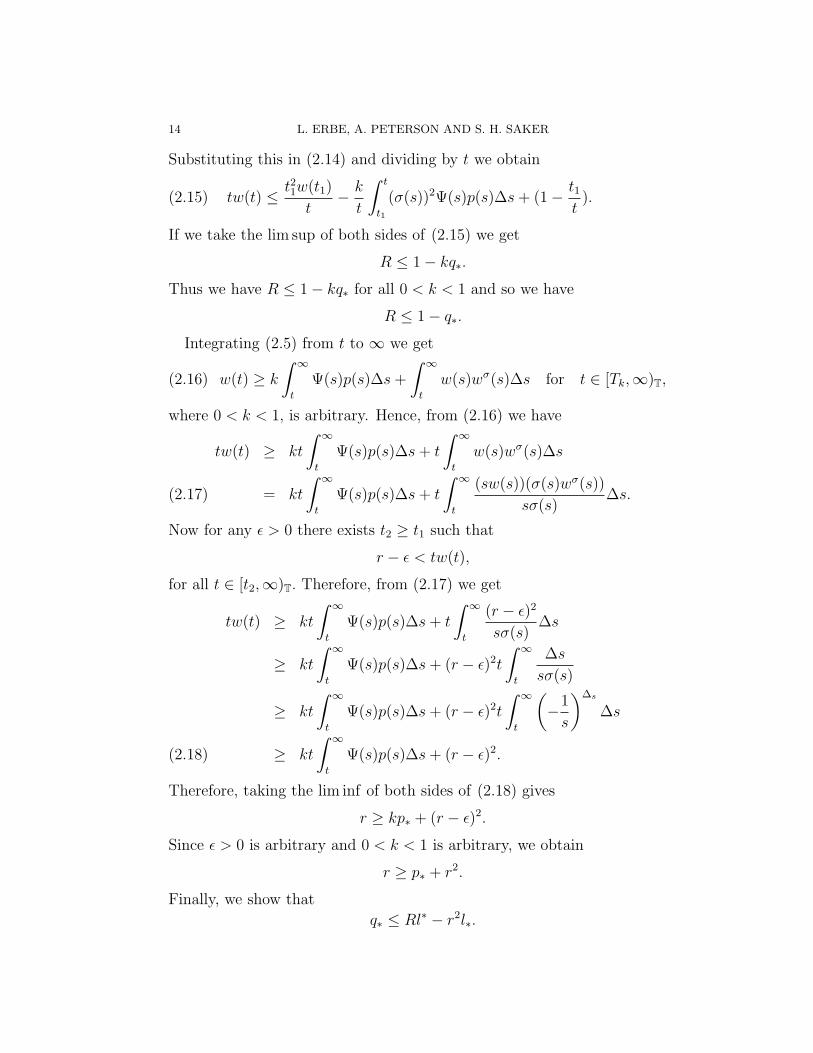
Substituting this in (2.14) and dividing by t we obtain
tw(t) ≤ t21w(t1)
t− k
t
∫ t
t1
(σ(s))2Ψ(s)p(s)∆s + (1− t1t).(2.15)
If we take the lim sup of both sides of (2.15) we get
R ≤ 1− kq∗.
Thus we have R ≤ 1− kq∗ for all 0 < k < 1 and so we have
R ≤ 1− q∗.
Integrating (2.5) from t to ∞ we get
(2.16) w(t) ≥ k
∫ ∞
t
Ψ(s)p(s)∆s +
∫ ∞
t
w(s)wσ(s)∆s for t ∈ [Tk,∞)T,
where 0 < k < 1, is arbitrary. Hence, from (2.16) we have
tw(t) ≥ kt
∫ ∞
t
Ψ(s)p(s)∆s + t
∫ ∞
t
w(s)wσ(s)∆s
= kt
∫ ∞
t
Ψ(s)p(s)∆s + t
∫ ∞
t
(sw(s))(σ(s)wσ(s))
sσ(s)∆s.(2.17)
Now for any ε > 0 there exists t2 ≥ t1 such that
r − ε < tw(t),
for all t ∈ [t2,∞)T. Therefore, from (2.17) we get
tw(t) ≥ kt
∫ ∞
t
Ψ(s)p(s)∆s + t
∫ ∞
t
(r − ε)2
sσ(s)∆s
≥ kt
∫ ∞
t
Ψ(s)p(s)∆s + (r − ε)2t
∫ ∞
t
∆s
sσ(s)
≥ kt
∫ ∞
t
Ψ(s)p(s)∆s + (r − ε)2t
∫ ∞
t
(−1
s
)∆s
∆s
≥ kt
∫ ∞
t
Ψ(s)p(s)∆s + (r − ε)2.(2.18)
Therefore, taking the lim inf of both sides of (2.18) gives
r ≥ kp∗ + (r − ε)2.
Since ε > 0 is arbitrary and 0 < k < 1 is arbitrary, we obtain
r ≥ p∗ + r2.
Finally, we show that
q∗ ≤ Rl∗ − r2l∗.
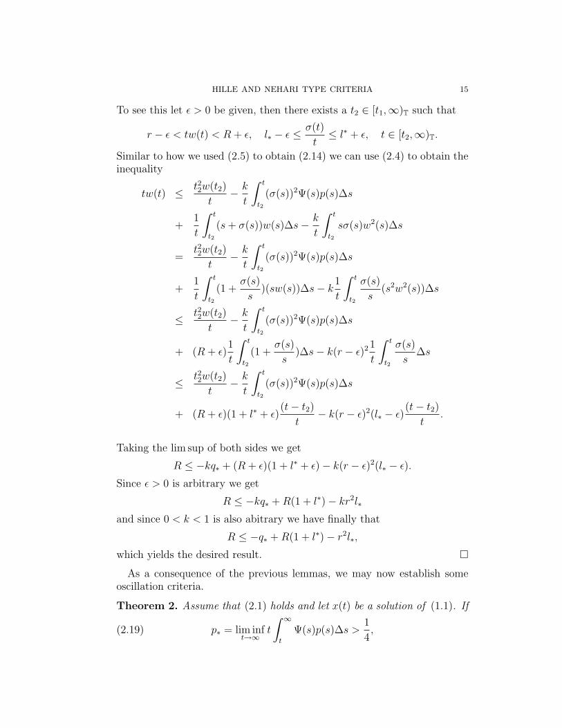
HILLE AND NEHARI TYPE CRITERIA 15
To see this let ε > 0 be given, then there exists a t2 ∈ [t1,∞)T such that
r − ε < tw(t) < R + ε, l∗ − ε ≤ σ(t)
t≤ l∗ + ε, t ∈ [t2,∞)T.
Similar to how we used (2.5) to obtain (2.14) we can use (2.4) to obtain theinequality
tw(t) ≤ t22w(t2)
t− k
t
∫ t
t2
(σ(s))2Ψ(s)p(s)∆s
+1
t
∫ t
t2
(s + σ(s))w(s)∆s− k
t
∫ t
t2
sσ(s)w2(s)∆s
=t22w(t2)
t− k
t
∫ t
t2
(σ(s))2Ψ(s)p(s)∆s
+1
t
∫ t
t2
(1 +σ(s)
s)(sw(s))∆s− k
1
t
∫ t
t2
σ(s)
s(s2w2(s))∆s
≤ t22w(t2)
t− k
t
∫ t
t2
(σ(s))2Ψ(s)p(s)∆s
+ (R + ε)1
t
∫ t
t2
(1 +σ(s)
s)∆s− k(r − ε)2 1
t
∫ t
t2
σ(s)
s∆s
≤ t22w(t2)
t− k
t
∫ t
t2
(σ(s))2Ψ(s)p(s)∆s
+ (R + ε)(1 + l∗ + ε)(t− t2)
t− k(r − ε)2(l∗ − ε)
(t− t2)
t.
Taking the lim sup of both sides we get
R ≤ −kq∗ + (R + ε)(1 + l∗ + ε)− k(r − ε)2(l∗ − ε).
Since ε > 0 is arbitrary we get
R ≤ −kq∗ + R(1 + l∗)− kr2l∗
and since 0 < k < 1 is also abitrary we have finally that
R ≤ −q∗ + R(1 + l∗)− r2l∗,
which yields the desired result. �
As a consequence of the previous lemmas, we may now establish someoscillation criteria.
Theorem 2. Assume that (2.1) holds and let x(t) be a solution of (1.1). If
(2.19) p∗ = lim inft→∞
t
∫ ∞
t
Ψ(s)p(s)∆s >1
4,

16 L. ERBE, A. PETERSON AND S. H. SAKER
then x(t) is oscillatory or satisfies limt→∞ x(t) = 0.
Proof. Suppose that x(t) is a nonoscillatory solution of equation (1.1) withx(t) > 0 on [t1,∞)T. Then if part (I) of Lemma 1 holds, let w(t) be asdefined in Lemma 5. From Lemma 7 we obtain
p∗ ≤ r − r2 ≤ 1
4
which contradicts (2.19). Now if part (II) of Lemma (1) holds, then byLemma 3, limt→∞ x(t) = 0. This completes the proof. �
Theorem 3. Assume that (2.1) holds and let x(t) be a solution of (1.1). If
(2.20) q∗ = lim inft→∞
1
t
∫ t
t0
σ(s)h2(s, t0)p(s)∆s >l∗
1 + l∗,
then x(t) is oscillatory or satisfies limt→∞ x(t) = 0.
Proof. From Lemma 7 we have that
q∗ ≤ min{1−R,Rl∗ − r2l∗} ≤ min{1−R,Rl∗}
which implies that q∗ ≤ l∗
1+l∗, which is a contradiction to (2.20). �
Theorem 4. Assume (2.1) holds, 0 ≤ p∗ ≤ 14, and
q∗ >l∗ − (1
2− p∗ − 1
2
√1− 4p∗) l∗
1 + l∗.(2.21)
Then every solution of (1.1) is oscillatory or satisfies limt→∞ x(t) = 0.
Proof. First we use the fact that a := p∗ ≤ r − r2 to get that
r ≥ r0 :=1
2−√
1− 4a
2,
and so using (2.12),
q∗ ≤ min{1−R, l∗R− r2l∗}≤ min{1−R, l∗R− r2
0l∗},
for r0 ≤ R ≤ 1. Note that
1−R = l∗R− r20l∗,
when
R = R0 :=1 + r2
0l∗1 + l∗
,
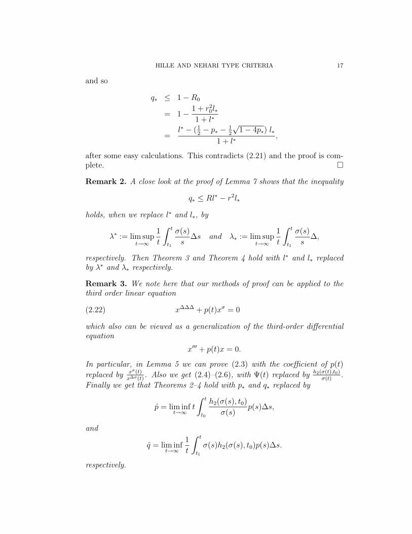
HILLE AND NEHARI TYPE CRITERIA 17
and so
q∗ ≤ 1−R0
= 1− 1 + r20l∗
1 + l∗
=l∗ − (1
2− p∗ − 1
2
√1− 4p∗) l∗
1 + l∗,
after some easy calculations. This contradicts (2.21) and the proof is com-plete. �
Remark 2. A close look at the proof of Lemma 7 shows that the inequality
q∗ ≤ Rl∗ − r2l∗
holds, when we replace l∗ and l∗, by
λ∗ := lim supt→∞
1
t
∫ t
t1
σ(s)
s∆s and λ∗ := lim sup
t→∞
1
t
∫ t
t1
σ(s)
s∆,
respectively. Then Theorem 3 and Theorem 4 hold with l∗ and l∗ replacedby λ∗ and λ∗ respectively.
Remark 3. We note here that our methods of proof can be applied to thethird order linear equation
x∆∆∆ + p(t)xσ = 0(2.22)
which also can be viewed as a generalization of the third-order differentialequation
x′′′ + p(t)x = 0.
In particular, in Lemma 5 we can prove (2.3) with the coefficient of p(t)
replaced by xσ(t)x∆σ(t)
. Also we get (2.4)–(2.6), with Ψ(t) replaced by h2(σ(t),t0)σ(t)
.
Finally we get that Theorems 2–4 hold with p∗ and q∗ replaced by
p = lim inft→∞
t
∫ t
t0
h2(σ(s), t0)
σ(s)p(s)∆s,
and
q = lim inft→∞
1
t
∫ t
t1
σ(s)h2(σ(s), t0)p(s)∆s.
respectively.
18 L. ERBE, A. PETERSON AND S. H. SAKER
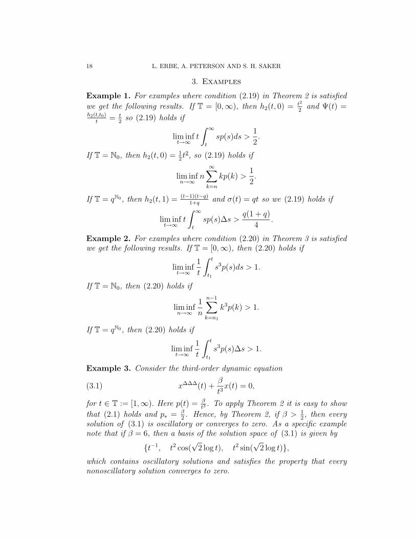
3. Examples
Example 1. For examples where condition (2.19) in Theorem 2 is satisfied
we get the following results. If T = [0,∞), then h2(t, 0) = t2
2and Ψ(t) =
h2(t,t0)t
= t2
so (2.19) holds if
lim inft→∞
t
∫ ∞
t
sp(s)ds >1
2.
If T = N0, then h2(t, 0) = 12t2, so (2.19) holds if
lim infn→∞
n∞∑
k=n
kp(k) >1
2.
If T = qN0, then h2(t, 1) = (t−1)(t−q)1+q
and σ(t) = qt so we (2.19) holds if
lim inft→∞
t
∫ ∞
t
sp(s)∆s >q(1 + q)
4.
Example 2. For examples where condition (2.20) in Theorem 3 is satisfiedwe get the following results. If T = [0,∞), then (2.20) holds if
lim inft→∞
1
t
∫ t
t1
s3p(s)ds > 1.
If T = N0, then (2.20) holds if
lim infn→∞
1
n
n−1∑k=n1
k3p(k) > 1.
If T = qN0, then (2.20) holds if
lim inft→∞
1
t
∫ t
t1
s3p(s)∆s > 1.
Example 3. Consider the third-order dynamic equation
(3.1) x∆∆∆(t) +β
t3x(t) = 0,
for t ∈ T := [1,∞). Here p(t) = βt3
. To apply Theorem 2 it is easy to show
that (2.1) holds and p∗ = β2. Hence, by Theorem 2, if β > 1
2, then every
solution of (3.1) is oscillatory or converges to zero. As a specific examplenote that if β = 6, then a basis of the solution space of (3.1) is given by
{t−1, t2 cos(√
2 log t), t2 sin(√
2 log t)},which contains oscillatory solutions and satisfies the property that everynonoscillatory solution converges to zero.

HILLE AND NEHARI TYPE CRITERIA 19
We wish to next consider two examples illustrating condition (2.21).
Example 4. Let T = qN0 and let
p(t) :=α
th2(t, 1), 0 < α ≤ 1
4.
Then we have Ψ(t)p(t) = αtσ(t)
, so
p∗ = lim inft→∞
t
∫ ∞
t
Ψ(s)p(s)∆s
= α lim inft→∞
t
∫ ∞
t
∆s
sσ(s)= α,
and since (σ(t))2Ψ(t)p(t) = αq, we have
q∗ = lim inft→∞
1
t
∫ t
t1
(σ(s))2Ψ(s)p(s)∆s
= lim inft→∞
1
t
∫ t
t1
αq∆s
= αq > q = p∗.
Since l∗ = l∗ = q, we see that if q∗ > q1+q
, then Theorem 3 applies. That is,
if α > 11+q
, all solutions are oscillatory or converge to zero. If 0 < α ≤ 11+q
,
then condition (2.21) of Theorem 4 is equivalent to
q∗ = αq >q − (1
2− α− 1
2
√1− 4α)q
1 + q,
which in turn is equivalent to
α >(1
2+ α + 1
2
√1− 4α)
1 + q.
Solving this inequality gives
q >1 +
√1− 4α
2α.(3.2)
Therefore, for any 0 < α ≤ 11+q
, Theorem 4 implies that all solutions are
oscillatory or converge to zero if (3.2) holds. For example, if α = 18
and
q > 4 + 4√2≈ 6.82, then Theorem 4 applies and Theorem 3 does not apply
if 4 + 4√2
< q < 7.
Example 5. We let T = qN0 ∪ aqN0 where 1 < a < q < a2. Then
T = {1, a, q, aq, q2, aq2, · · · }.
20 L. ERBE, A. PETERSON AND S. H. SAKER
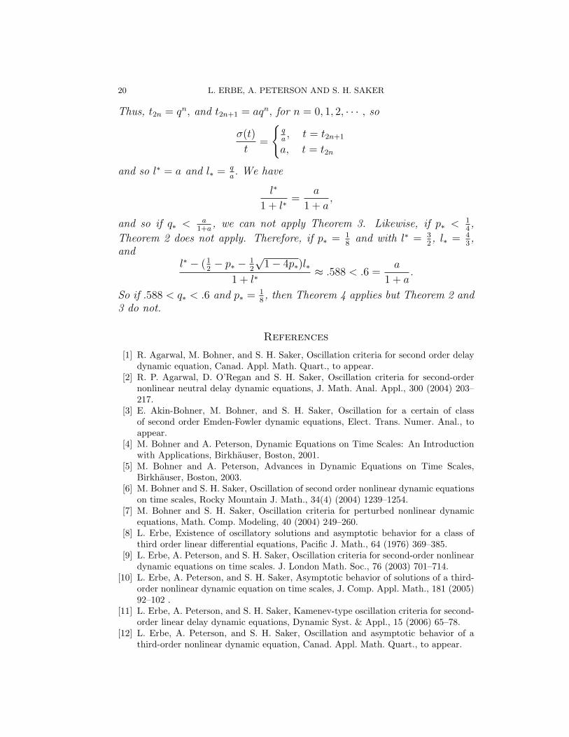
Thus, t2n = qn, and t2n+1 = aqn, for n = 0, 1, 2, · · · , so
σ(t)
t=
{qa, t = t2n+1
a, t = t2n
and so l∗ = a and l∗ = qa. We have
l∗
1 + l∗=
a
1 + a,
and so if q∗ < a1+a
, we can not apply Theorem 3. Likewise, if p∗ < 14,
Theorem 2 does not apply. Therefore, if p∗ = 18
and with l∗ = 32, l∗ = 4
3,
andl∗ − (1
2− p∗ − 1
2
√1− 4p∗)l∗
1 + l∗≈ .588 < .6 =
a
1 + a.
So if .588 < q∗ < .6 and p∗ = 18, then Theorem 4 applies but Theorem 2 and
3 do not.
References
[1] R. Agarwal, M. Bohner, and S. H. Saker, Oscillation criteria for second order delaydynamic equation, Canad. Appl. Math. Quart., to appear.
[2] R. P. Agarwal, D. O’Regan and S. H. Saker, Oscillation criteria for second-ordernonlinear neutral delay dynamic equations, J. Math. Anal. Appl., 300 (2004) 203–217.
[3] E. Akin-Bohner, M. Bohner, and S. H. Saker, Oscillation for a certain of classof second order Emden-Fowler dynamic equations, Elect. Trans. Numer. Anal., toappear.
[4] M. Bohner and A. Peterson, Dynamic Equations on Time Scales: An Introductionwith Applications, Birkhauser, Boston, 2001.
[5] M. Bohner and A. Peterson, Advances in Dynamic Equations on Time Scales,Birkhauser, Boston, 2003.
[6] M. Bohner and S. H. Saker, Oscillation of second order nonlinear dynamic equationson time scales, Rocky Mountain J. Math., 34(4) (2004) 1239–1254.
[7] M. Bohner and S. H. Saker, Oscillation criteria for perturbed nonlinear dynamicequations, Math. Comp. Modeling, 40 (2004) 249–260.
[8] L. Erbe, Existence of oscillatory solutions and asymptotic behavior for a class ofthird order linear differential equations, Pacific J. Math., 64 (1976) 369–385.
[9] L. Erbe, A. Peterson, and S. H. Saker, Oscillation criteria for second-order nonlineardynamic equations on time scales. J. London Math. Soc., 76 (2003) 701–714.
[10] L. Erbe, A. Peterson, and S. H. Saker, Asymptotic behavior of solutions of a third-order nonlinear dynamic equation on time scales, J. Comp. Appl. Math., 181 (2005)92–102 .
[11] L. Erbe, A. Peterson, and S. H. Saker, Kamenev-type oscillation criteria for second-order linear delay dynamic equations, Dynamic Syst. & Appl., 15 (2006) 65–78.
[12] L. Erbe, A. Peterson, and S. H. Saker, Oscillation and asymptotic behavior of athird-order nonlinear dynamic equation, Canad. Appl. Math. Quart., to appear.

HILLE AND NEHARI TYPE CRITERIA 21
[13] M. Hanan, Oscillation criteria for third order differential equations, Pacific J. Math.,11 (1961) 919–944.
[14] S. Hilger, Analysis on measure chains–a unified approach to continuous and discretecalculus, Results Math., 18 (1990) 18–56.
[15] E. Hille, Non-oscillation theorems, Trans. Amer. Math. Soc., 64 (1948) 234–252.[16] V. Kac and P. Cheung, Quantum Calculus, Universitext, Springer, New York, 2001.[17] W. Kelley and A. Peterson, Difference Equations: An Introduction With Applica-
tions, second edition, Harcourt/Academic Press, San Diego, 2001.[18] A. C. Lazar, The behavior of solutions of the differential equation y′′′ + p(x)y′ +
q(x)y = 0, Pacific J. Math., 17 (1966) 435–466.[19] W. Leighton, The detection of the oscillation of solutions of a second order linear
differential equation, Duke J. Math., 17 (1950) 57–62.[20] B. Mehri, On the conditions for the oscillation of solutions of nonlinear third order
differential equations, Cas. Pest Math., 101 (1976) 124–129.[21] Z. Nehari, Oscillation criteria for second-order linear differential equations, Trans.
Amer. Math. Soc., 85 (1957) 428–445.[22] S. H. Saker, Oscillation criteria of second-order half-linear dynamic equations on
time scales, J. Comp. Appl. Math., 177 (2005) 375–387.[23] S. H. Saker, Oscillatory behavior of linear neutral delay dynamic equations on time
scales, Kyungpook Math. J., to appear.[24] S. H. Saker, Oscillation of second-order nonlinear neutral delay dynamic equations
on time scales, J. Comp. Appl. Math., 177 (2005) 375–387.[25] S. H. Saker, Oscillation criteria for a certain class of second-order neutral delay
dynamic equations, Dynamics of Continuous, Discrete and Impulsive Systems SeriesB: Applications & Algorithms, to appear.
[26] S. H. Saker, New oscillation criteria for second-order nonlinear dynamic equationson time scales, Nonlin. Funct. Anal. Appl. (NFAA), to appear.
[27] S. H. Saker, On oscillation of second-order delay dynamic equations on tme scales,Austral. J. Math. Anal. Appl., to appear.
[28] S. H. Saker, Oscillation of second-order neutral delay dynamic equations of EmdenFowler type, Dynam. Syst. Appl., to appear.
[29] V. Spedding, Taming Nature’s Numbers, New Scientist, July 19, 2003, 28–31.
Department of Mathematics, University of Nebraska-Lincoln, Lincoln,NE 68588-0130, U.S.A. [email protected], [email protected]
Department of Mathematics, Faculty of Science, Mansoura University,Mansoura, 35516, Egypt. [email protected]