hilbert spaces - penn engineering · 2002-09-04 · hilbert spaces our previous discussions have...

5

Hilbert Spaces

Our previous discussions have been concerned with algebra. The represen-tation of systems (quantities and their interrelations) by abstract symbolshas forced us to distill out the most significant and fundamental propertiesof these systems. We have been able to carry our exploration much deeperfor linear systems, in most cases decomposing the system models into setsof uncoupled scalar equations.

Our attention now turns to the geometric notions of length and angle.These concepts, which are fundamental to measurement and comparisonof vectors, complete the analogy between general vector spaces and thephysical three-dimensional space with which we are familiar. Then ourintuition concerning the size and shape of objects provides us with valu-able insight. The definition of length gives rigorous meaning to ourprevious heuristic discussions of an infinite sequence of vectors as a basisfor an infinite-dimensional space. Length is also one of the most widelyused optimization criteria. We explore this application of the concept oflength in Chapter 6. The definition of orthogonality (or angle) allows us tocarry even further our discussion of system decomposition. To this point,determination of the coordinates of a vector relative to a particular basishas required solution of a set of simultaneous equations. With orthogonalbases, each coordinate can be obtained independently, a much simplerprocess conceptually and, in some instances, computationally.

5.1 Inner Products

The dot product concept is familiar from analytic geometry. If x = ([r,@and y = (qr,r/& are two vectors from $k2, the dot product between xand y is defined by

(5.1)

The length 11 XII of the vector x is defined by

(5.2)

237

238 Hilbert Spaces

The angle between the vectors x and y is defined in terms of the dotproduct between the normalized vectors:

(5.3)

Example 1. The Dot Product in 3’. Let x = (1,1) and y = (2,0). Then = 2,

11x11= fi, llyll=2, and cos+= l/e (or +=45”)). Figure 5.1 is an arrow spaceequivalent of this example.

Figure 5.1. Arrow vectors corresponding to Example 1.

It is apparent from Example 1 that (5.3) can be interpreted, in terms ofthe natural correspondence to arrow space, as a definition of the dotproduct (as a function of the angle between the vectors):

(5.4)

where [[xl1 cos+ is the length of the projection of x on y along theperpendicular to y. The following properties of the dot product seemfundamental:

1. Length is non-negative; that is,

with equality if and only if x = 8

2. The magnitude of C#B (or cos+) is independent of the order of x andy; that is,

x*y=y*x

Sec. 5.1 Inner Products 239

3. The length of cx equals ICI times the length of x, for any scalar c;that is,

cx*cx=c2(x*x)

4. In order that (5.4) be consistent with the rules for addition ofvectors, the dot product must be distributive over addition (see Figure 5.2);that is,

We now extend the dot product to arbitrary vector spaces with real orcomplex scalars in a manner which preserves these four properties.

Definition. An inner product (or scalar product) on a real or complexvector space 1/ is a scalar-valued function of the ordered pair ofvectors x and y such that:

1. (x,x> > 0, with equality if and only if x = 82. (x,y) = (y,x) (the bar denotes complex conjugation).3. ~~~~~+~2~2~Y~=~~~~~~Y~+~2~~2~Y~

It follows that (y,c,x, + c2x2) = Ci(y,x,) + ?2(y,x2). We describe these pro-perties by saying that an inner product must be (1) positive definite, (2)hermitian symmetric, and (3) conjugate bilinear. Note that because of (2),(x,x) is necessarily real, and the inequality (1) makes sense. If the scalarsare real, the complex conjugation bar is superfluous.

Figure 5.2. Dot products are distributive over addition.

240

We define the norm (or length) of x by

Hilbert Spaces

llxll g v?Lq (5.5)

When (x, y) is real, we can define the angle # between x and y by

A bY>cosq = llxll

Practicallytwo cases:

speaking, we are interested in the angle + only in the following

(x, y> = 0 (x and y are said to be orthogonal) (5.6)

<X,Y> = 2 llxll llyll (x and y are said to be collinear) (5.7)

Example 2. The Standard Inner Product for en and an. The standard innerproduct for (I?” (and %’ ) is defined by

(5.8)

where & and vi are the elements of x and y, respectively. Of course, the complexconjugate bar is superfluous for $Ln. This inner product is simply the extension ofthe dot product to complex spaces and n dimensions. Consider the vector ( i) in (?‘;

The complex conjugation in (5.8) is needed in order to keep lengths non-negativefor complex scalars.

Example 3. The Standard Inner Product for ?IRf x ’ and %Rnx’. The standardinner product for %I,:” * is defined by

(x,y) 4 y'x (5.9)

Again, if only real scalars are involved, the conjugate is unnecessary. For instance,if x = (1 2 4)T and y = (-1 3 2)T in tX3xx, then, by (5.9),

Example 4. The Standard Inner Product for Function Spaces. The standard inner


product for a function space such as 9’ (a, 6) or (?. (a, b) is defined by

<f,g) 2 /“red s(t) dta

(5.10)

for each f and g in the space. We usually deal only with real functions and ignorethe complex conjugation. Consider the function f(t) = 1 in (2 (0,l):

Any vector whose average value over the interval [0, l] is zero is orthogonal to f; for

s

1then (f, g) = (l)g(t)dt = 0. We easily verify, for the case of continuous functions

0and real scalars, that (5.10) possesses the properties of an inner product; by theproperties of integrals:(a) (f,f) = $ if*(t)dt > 0, with equality if and only if f(t)=0 for all t in [a,b];

(b) S :WMW = S :&YWt(4 s f: [Cl f* (9 + C2f2wl~w dt = ~1 S if ,OkW dt + c2 S :f,W&)dt

Example 5. The Standard Inner Product for a Space of Two-Dimensional Functions.Let e*@) denote the space of functions which are twice continuously differentiableover a two-dimensional region a. We define an inner product for (Z*(G) by

(f, id A J,fbk(p) dp (5.11)

where p = (s , t), an arbitrary point in 52.

An inner product assigns a real number (or norm) to each vector in thespace. The norm provides a simple means for comparing vectors inapplications. Example 1 of Section 3.4 is concerned with the state (orposition and velocity) of a motor shaft in the state space X2” ‘. In aparticular application we might require both the position and velocity toapproach given values, say, zero. As a simple measure of the nearness ofthe state to the desired position (e), we use the norm corresponding to(5.9):

where tr and t2 are the angular position and velocity of the motor shaft atinstant t. However, there is no inherent reason why position and velocityshould be equally important. We might be satisfied if the velocity stayedlarge as long as the position of the shaft approached the target position

242 Hilbert Spaces

5, = 0. In this case, some other measure of the performance of the system-1

would be more appropriate. The following measure weights & moreheavily than t2.

This new measure is just the norm associated with the following weightedinner product for %2x ’ :

where x = ([, t2)’ and y = (qt 71~)~. We generally select that inner productwhich is most appropriate to the purpose for which it is to be used.

Example 6. A Weighted Inner Product for Function Spaces. An inner product ofthe following form is often appropriate for such spaces as 9 ( a , b) and &?(a, b):

(5.12)

If the weight function is w(t)= 1, (5.12) reduces to the standard inner product(5.10). The weight w(t) = e’ might be used to emphasize the values of functions forlarge t and deemphasize the values for t small or negative.

Example 7, A Weighted Inner Product for 3’. Let x = (ti, c2) and y = (r)i,~z) bearbitrary vectors in CR*. Define the inner product on %* by

(5.13)

We apply this inner product to the vectors x = (1,1) and y = (2,0), the same vectorsto which we previously applied the standard (or dot) inner product: (x, y) = 0,lixll= 1, and llyll = 1. The same vectors which previously were displaced by 45°(Figure 5.1) are, by definition (5.13), orthogonal and of unit length. We see that(5.13) satisfies the properties required of an inner product:

1. By completing the square, we find

<x,x)= $G -t*)2+g > 0

with equality if and only if & = t2= 0;2. Since the coefficients for the cross-product terms are equal,

<X,Y> = (YJQ


3. We rewrite (5.13) as

Then, by the linearity of matrix multiplication,

<VI + ~2x29 Y> = Y~Q(c,x, + ~2x2)

= clyTQxl + c2yTQx2

=cIhY)+c*<x29Y)

The last two examples suggest that we have considerable freedom inpicking inner products. Length and orthogonality are, to a great extent,what we define them to be. Only if we use standard inner products in $K3do length and orthogonality correspond to physical length and 90° angles.Surprisingly, the concept suggested by (5.4) still holds in Example 7:I(x,y>I is the product of llyll and the norm of the projection of x on y alongthe direction orthogonal [in the sense of (5.13)] to y. The sign of (x, y) ispositive if the projection of x on y is in the same direction as y ; if theprojection is in the opposite direction, the sign is negative.

Exercise 1. Let x = (0,1) and y = (1,0) in a2. Define the inner product inq2 by (5.13). Show that the projection of x on y along the directionorthogonal to y is the vector (-1,0). Verify that (x, y) is correctlydetermined by the above rule which uses the projection of x on y.

An inner product space (or pre-Hilbert space) is a vector space on whicha particular inner product is defined. A real inner product space is called aEuclidean space. A unitary space is an inner product space for which thescalars are the complex numbers. We will often employ the symbols ‘?Rnand Xnxl to represent the Euclidean spaces consisting of the real vectorspaces ‘Zion and ‘%,nx ’ together with the standard inner products (5.8) and(5.9), respectively. Similarly, we use ?? (a, b), 6? (a, b), etc. to represent realEuclidean function spaces which make use of the standard inner product(5.10). Whereever we use a different (nonstandard) inner product, wemention it explicitly.

Matrices of Inner Products

To this point, we have not used the concept of a basis in our discussion ofinner products. There is no particular basis inherent in any inner productspace, although we will find some bases more convenient than others. Wefound in Chapter 2 that by picking a basis % for an n-dimensional space

244 Hilbert Spaces

V we can represent vectors x in Ir by their coordinates [xl, in the“standard” space $!Kn x ’ ; moreover, we can represent a linear operator Ton V by a matrix manipulation of [xl,, multiplication by [T]%,, . It seemsonly natural that by means of the same basis we should be able to convertthe inner product operation to a matrix manipulation. We proceed bymeans of an example.

Let x = (S,,&) and y = (r)i,qJ be general vectors in the vector space Ck2.

Let (x, y) represent the inner product (5.13). We select % A & , thestandard basis for a2. Then using the bilinearity of the inner product,

On the surface, we appear to have returned to the defining equation (5.13),but the meaning of the equation is now different; ti and qi now representcoordinates [or multipliers of the vectors (1,0) and (0,1)] rather thanelements of the vectors x and y. We rewrite the last line of the equation as

We have converted the inner product operation to a matrix multiplication.We call Q6 the matrix of the inner product relative to the basis & . Insimilar fashion, any inner product on a finite-dimensional space can berepresented by a matrix.

Let % h {x1 , … , xn} be a basis for an inner product space V. Then

n nX= c a,x, and Y = C $xj

k-l j-1


By the argument used for the special case above,

Cx, Y> = < C akxk, If bjxj)k j

(5.14)

We refer to QX as the matrix of the inner product ( l , .) relative to thebasis %. It is evident that

(5.15)

We can use (5.15) directly to generate the matrix of a given inner productrelative to a particular basis. The matrix (5.15) is also known as the Grammatrix for the basis % ; the matrix consists in the inner products of allpairs of vectors from the basis.

Exercise 2. Use (5.15) to generate the matrix of the inner product (5.13)relative to the standard basis for 9L2.

From (5.14), (5.15), and the definition of an inner product we deducethat a Gram matrix, or a matrix of an inner product, has certain specialproperties which are related to the properties of inner products:

1. Since (Xk,Xj)=(Xj,Xk), Qx =0x’.

2 . The inner product is positive definite; denoting z A [xl%, we findZTQx z > 0 for all z in m x ‘, with equality if and only if z = 8.

We describe these matrix properties by saying QX is (1) hermitian sym-metric* and (2) positive definite. For a given basis, the set of all possible

*If Qc issymmetric.

real, the complex conjugate is superfluous. Then, if QX=QaT, we say Qa is

246 Hilbert Spaces

inner products on an n-dimensional space V is equivalent to the set ofpositive-definite, hermitian symmetric n x n matrices. This fact indicatesprecisely how much freedom we have in picking inner products. In point offact, (5.14) can be used in defining an inner product for Ir. We will exploitit in our discussion of orthogonal bases in the next section. A method fordetermining whether or not a matrix is positive definite is described inP&C 5.9.

Exercise 3. Any inner product on the real space ‘%VLnx ’ is of the form

(x, y j k y’Qx for some symmetric positive-definite matrix Q. Theanalogous definition for a real function space on the interval [a , b] is

Kg> b JbSbk(t.s)f(t)g(s)dFdia a

What properties must the kernel function k possess in order that thisequation define a valid inner product (see P&C 5.30)? Show that ifk(t,s) = cc)( t)8 (t - s), then the inner product reduces to (5.12).

5.2 Orthogonality

The thrust of this section is that orthogonal sets of vectors are not onlylinearly independent, but also lead to independent computation ofcoordinates. A set S of vectors is an orthogonal set if the vectors arepairwise orthogonal. If, in addition, each vector in S has unit norm, theset is called orthonormal. The two vectors of Example 1 (below) form anorthonormal set relative to the inner product (5.13). The standard basis foran is an orthonormal set relative to the standard inner product. Suppose

the set !XA{(x i,. . .,x,} is orthogonal. It follows that each vector in X isorthogonal to (and linearly independent of) the space spanned by the othervectors in the set; for example,

If ‘%, is an orthogonal basis for an n-dimensional space ‘v, then for anyvector x in 71‘, x = 2: = ickxk and

(x, xk) = (c$l + ’ ’ ’ + c,x,, x,)

= c,<xI,xk) + ’ ’ ’ + ck(xk,xk) + ’ ’ * + c,(x,,,x~)

= dxk, x,>

Sec. 5.2 Orthogonality 247

Thus the kth coordinate of x relative to the orthogonal basis % is

(X,Xk)Ck = -

(%Xk)(5.16)

Each coordinate can be determined independently using (5.16). The set ofsimultaneous equations which, in previous chapters, had to be solved inorder to find coordinates is not necessary in this case. Inherent in the“orthogonalizing” inner product is the computational decoupling of thecoordinates. If, in fact, the vectors in 5% are orthonormal, the denominatorin (5.16) is 1, and

x= Ii (JWJX,k=l

(5.17)

Equation (5.17) is known as a generalized Fourier series expansion (ororthonormal expansion) of x relative to the orthonormal basis !X . The kthcoordinate, (x,x&, is called the kth Fourier coefficient of x relative to theorthonormal basis ‘X. We will have little need to distinguish between(5.17) and the orthogonal expansion which uses the coefficients (5.16). Wewill also refer to the latter expansion as a Fourier series expansion, and to(5.16) as a Fourier coefficient.

Example 1. Independent Computation of Fourier Coefficients. From Example 7

of the previous section we know that the vectors xl b (1,1) and x2 i (2,0) form abasis for 9L2 which is orthonormal relative to the inner product (5.13). Let x = (2,1).Then by (5.17) we know that

x=(2,1)=c,(1,1)+c2(2,0)

where cl = (x, xl> = ((2, l), (1,l)) = 1 and c2 = (x, x2) = ((2, I), (2,o)) = ;.

Gram-Schmidt Orthogonalization Procedure

The Gram-Schmidt procedure is a technique for generating anorthonormal basis. Suppose x1 and x2 are independent vectors in the spaceCiL2 with the standard inner product (dot product). (See the arrow spaceequivalent in Figure 5.3.) We will convert this pair of vectors to anorthogonal pair of vectors which spans the same space. The vector x2

decomposes uniquely into a pair of components, one collinear with x1 andthe other orthogonal to x1. The collinear component is Ilx,ll cos+ times theunit vector in the direction of x1; using the expression (5.4) for the dot

2 4 8 Hilbert Spaces

Figure 5.3. Gram-Schmidt orthogonalization in arrow space.

product, we convert this collinear vector to the form

Define zt AxI and Then z2 is orthogonal to z1 ,and {z1, z2 } is an orthogonal set which spans the same space as {x1, x2 }. Wecan normalize these vectors to obtain an orthonormal set {y l,y2} whichalso spans the same space: yl=zI/IIzlll, and y2=z2/~~z2~~.

The procedure applied to the pair of vectors in C!k2 above can be used toorthogonalize a finite number of vectors in any inner product space.Suppose we wish to orthogonalize a set of vectors {x 1 , … , xn } from someinner product space V. Assume we have already replaced x1 , … , xk by anorthogonal set z1 , … , zk which spans the same space as x1 , … , xk (imaginek = 1). Then xk + 1 decomposes uniquely into a pair of components, one inthe space spanned by {z1 , … , zk } and the other (zk +1) orthogonal to

z1 , … , zk. Thus zk +1 must satisfy

xk+l=(c$~+“’ +ckzk)+zk+l

Since the set {z1 , ... , zk + 1 } must be orthogonal, and therefore a basis forthe space it spans, the coefficients {c j} are determined by (5.16):

Therefore,

(5.18)


Exercise 1. Verify that zk + 1 as given in (5.18) is orthogonal to zj forj = l, ... , k. How do we know the “orthogonal” decomposition of xk+1 isunique?

Starting with z1 = x1 and using (5.18) for k = 1, … , n-1, we generate anorthogonal basis for the space spanned by {x1 , … , xn }. The procedure canbe applied to any finite set of vectors, independent or not; any dependen-cies will be eliminated (P&C 5.14). Thus we can obtain an orthogonalbasis for a vector space by applying (5.18) to any set of vectors whichspans the space. The application of (5.18) is referred to as the Gram-Schmidt orthogonalization procedure. It requires no additional effort tonormalize the vectors at each step, obtaining Yj = Zj/llZjll; then (5.18)becomes

zk+l=xk+l - Ii CxIc+l,Yj)Yj (5.19)j-l

Numerical accuracy and techniques for retaining accuracy in Gram-Schmidt orthogonalization are discussed in Section 6.6.

Example 2. Gram-Schmidt Orthogonalization in a Function Space. Define

fk(t) = t k in the space 9 (-1,1) with the standard inner product

We will apply the Gram-Schmidt procedure to the first few functions in the set{f 0 , f1, f2 , …}. Using (5.18), with appropriate adjustments in notation, we let g0 (t)= f 0 (t ) = 1 and

But (f,,g,,)= J’!,(t)(l)dt = 0. Therefore, g1 (t) = f1 (t) = t, and g1 is orthogonal to g0 .Again using (5.18),

The inner products are

250 Hilbert Spaces

Therefore, g2(t)= t2- f, and g2 is orthogonal to g1 and g0. We could continue, if wewished, to generate additional vectors of the orthogonal set {g0 , g 1 , g2 , …}. Thefunctions {gk } are known as orthogonal polynomials. Rather than normalize these

orthogonal polynomials, we adjust their length as follows: define pk b gk/gk(l) sothat pk (1)= 1. The functions {p 0 , p1 , p2 , . . . } so defined are known as the Legendrepolynomials. (These polynomials are useful for solving partial differential equationsin spherical coordinates.) Thus p0 (t) = go (t) = 1, pl(t) = g1 (t) = t, and p2 (t) = g2 (t)/g 2(1) = (3 t 2-1)/2. A method of computing orthogonal polynomials which uses lesscomputation than the Gram-Schmidt procedure is described in P&C 5.16.

Orthogonal Projection

The orthogonal complement of a set S of vectors in a vector space ‘v is theset s L of all vectors in ?r which are orthogonal to every vector in s . Forexample, the orthogonal complement of the vector x1 of Figure 5.3 is thesubspace spanned by z2. On the other hand, the orthogonal complement ofspan{z2 } is not the vector x1, but rather the space spanned by x1. Anorthogonal complement is always a subspace.

Example 3. An Orthogonal Complement in Suppose the set S in thestandard inner product space LZ (0,l) consists of the single function f1 (t ) = 1. ThenS L is the set of all functions whose average is zero; that is, those functions g forwhich

(f,,g)= ~‘(1)&)dr=0

As part of our discussion of the decomposition of a vector space ?r intoa direct sum, II‘ = W1 Cl3 %,, we introduced the concept of a projection onone of the subspaces along the other (Section 4.1). In the derivation of(5.18) we again used this concept of projection. In particular, each time weapply (5.18), we project a vector xk +1 onto the space spanned by{ z1 ,… , zk } along a direction orthogonal to zl, … , zk (Figure 5.3). Suppose

we define G2IT A span{z1 , . . . , zk }. Then any vector which is orthogonal tozl ,…, zk is in G2LIL, the orthogonal complement of W. The only vectorwhich is in both W and ‘?.l!l is the vector 8. Since the vector xk+1 of(5.18) can be any vector in ?r, the derivation of (5.18) constitutes a proof(for finite-dimensional V)* that

(5.20)

*The projection theorem (5.20) also applies to certain infinite-dimensional spaces. Specifi-cally, it is valid for any (complete) subspace W of a Hilbert space Y. See Bachman andNarici [5.2, p. 172]. These infinite-dimensional concepts (Hilbert space, subspace, andcompleteness) are discussed in Section 5.3.


That is, any vector in ‘v can be decomposed uniquely into a pair ofcomponents, one in % and the other orthogonal to ‘% . The projection ofa vector x on a subspace % along %-‘- is usually referred to as theorthogonal projection of x on %. Equation (5.20), which guarantees theexistence of orthogonal projections, is sometimes known as the projectiontheorem. This theorem is one of the keys to the solution of the least-squareoptimization problems explored in Chapter 6.

It is apparent from (5.18) that the orthogonal projection X~ of anarbitrary vector x in V onto the subspace ‘?IT spanned by the orthogonalset { z l, ... , z k } is

(5.21)

We can also write (5.21) in terms of the normalized vectors {y1, . . . , yk } of(5.19):

%Js = i bYj)Yjj=l

(5.22)

Equation (5.22) expresses xGuc as a partial Fourier series expansion, an“attempted” expansion of x in terms of an orthonormal basis for thesubspace on which x is projected. If x - Et= ,(x, yi)yj # 8, we know that theorthonormal basis for % is not a basis for the whole space ‘v. It isevident that an orthonormal set {yi} is a basis for a finite-dimensionalspace ‘v if and only if there is no nonzero vector in V which is orthogonalto { yi }. We can compute the orthogonal projection of x on % withoutconcerning ourselves with a basis for the orthogonal complement %I. Wecan do so because a description of ‘%l is inherent in the inner product.Clearly, Gram-Schmidt orthogonalization, orthogonal projection, andFourier series are closely related. Equation (5.22), or its equivalent, (5.21),is a practical tool for computing orthogonal projections on finite-dimensional subspaces.

Example 4. Computation of an Orthogonal Projection. Let %!Y be that subspaceof the standard inner product space a3 which is spanned by {x1 ,x2 }, wherex1 = (1,0,1) and x2 = (0,1,1). We seek the orthogonal projection of x = (0,0,2) onG2Lc. We first use the Gram-Schmidt procedure to orthogonalize the set {x1 ,x2 };then we apply (5.21). By (5.18), z1 = x1 = (1,0,1) and

252 Hilbert Spaces

By (5.21),

Orthonormal Eigenvector Bases for Finite-Dimensional Spaces

In (4.13) we solved the operator equation TX = y by means of spectraldecomposition (or diagonalization). By representing the input vector y interms of its coordinates relative to a basis of eigenvectors, we convertedthe operator equation into a set of uncoupled scalar equations, andsolution for the output x became simple. Of course, even when theeigendata were known, a set of simultaneous equations was required inorder to decompose y. We now explore the solution of equations by meansof an orthonormal basis of eigenvectors. The orthonormality allows us todetermine independently each eigenvector component of the input; thesolution process is then completely decoupled.

Let T have eigendata {Xi} and {z i}, and let {z 1 , . . . , zn } be a basis for thespace V on which T operates. (Then T must be diagonalizable.) Further-more, suppose T is invertible; that is, Xj#O. We solve the operatorequation Tx = y as follows. The vectors x and y can be expanded as

and

The coordinates { c j} can be determined from y; the numbers { d j } arecoordinates of the unknown vector x. Inserting these eigenvector ex-pansions into the operator equation, we obtain

o r

C (d,h, - Cj)Zj= 8

Since the vectors zj are independent, 4 = cj/hi, and the solution to theoperator equation is

(5.23)


Suppose the eigenvector basis {z1, … , zn } is orthonormal relative to theinner product on V. Then the eigenvector expansion of y can be expressedas the Fourier expansion

and the solution (5.23) becomes

(5.24)

Each component of (5.24) can be evaluated independently.If T is not invertible, (5.24) requires division by a zero eigenvalue. The

eigenvectors for the zero eigenvalue form a basis for nullspace(T ). Theremaining eigenvectors are taken by T into range(T), and in fact form abasis for range(T). To avoid division by zero in (5.24), we split the space:y = nullspace(T) range( T ). The equation Tx = y has no solution unless yis in range(T) (or cj = 0 for i corresponding to a zero eigenvalue); since theeigenvectors are assumed to be orthonormal, an equivalent statement isthat y must be orthogonal to nullspace(T ). Treating the eigenvectorscorresponding to zero eigenvalues separately, we replace the solution x in(5.23)-(5.24) by

(5.25)

where x0 is an arbitrary vector in nullspace(T). The first portion of (5.25) isa particular solution to the equation Tx = y. The second portion, x0, is thehomogeneous solution. The undetermined coefficients di in the sum whichconstitutes x0 are indicative of the freedom in the solution owing to thenoninvertibility of T.

What fortunate circumstances will allow us to find an orthonormal basisof eigenvectors? .The eigenvectors are properties of T; they cannot beselected freely. Assume there are enough eigenvectors of T to form a basisfor the space. Were we to orthogonalize an eigenvector basis using theGram-Schmidt procedure, the resulting set of vectors would not be eigen-vectors. However, we have considerable freedom in picking inner products.

254 Hilbert Spaces

In point of fact, since the space is finite dimensional, we can select theinner product to make any particular basis orthonormal.

The key to selection of inner products for finite-dimensional spaces is(5.14), the representation of inner products of vectors in terms of theircoordinates. Let the basis % be {z 1 , … , zn }, the eigenvectors of T. Weselect the matrix of the inner product, Qn, such that the basis vectors areorthonormal. By (5,15), if % is to be orthonormal, QX satisfies

(5.26)

or QX = I. By (5.14), this matrix defines the following inner product on V:

(5.27)

The expression (5.27) of an inner product in terms of coordinates relativeto an orthonormal basis is called Parseval’s equation. A basis % isorthonormal if and only if (5.27) is satisfied; that is, if and only if the innerproduct between any two vectors equals the standard inner product (inXnx ‘) between their coordinates relative to % .

Example 5. Solution of an Equation by Orthonormal Eigenvector Expansion.Suppose we define T: $I%‘-+ 9L2 by

[The same operator is used in the decomposition of Example 7, Section 4.1.] Theeigendata are At = 2, z1 = (1,0), A,=4, and z2 = (3,2). The pair of eigenvectors,

‘5% i {z1 , z2 }, is a basis for ?R2. We define the inner product for %2 by (5.27):

(x9 Y> = [Yl&ln

To make this definition more explicit, we find the coordinates of x and y; lety = alzl + a2 z2, or

y = hr/J = a1 (1,0) + a2 (3,2)

Solution (by row reduction) yields al = ql - 3v2/2 and a2= q2/2. Similarly, thecoordinates of x = (&,&) are c1 =[r - 3t2/2 and c2=t2/2. Thus we can express theinner product as


Relative to this inner product, the basis % is orthonormal. We solve the equationTx=T(&,~~)=(~~,~~)=Y using (5.24):

We have developed two basic approaches for analyzing a finite-dimensional, invertible, diagonalizable, linear equation: (a) operator inver-sion and (b) spectral decomposition (or eigenvector expansion). Bothmethods give explicit descriptions of the input-output relationship of thesystem for which the equation is a model. The spectral decompositionyields a more detailed description; therefore, it provides more insight thandoes inversion. If the eigenvector expansion is orthonormal, we also obtainconceptual and computational independence of the individual terms in theexpansion.

What price do we pay for the insight obtained by each of theseapproaches ? We take as a measure of computational expense theapproximate number of multiplications required to analyze an n X n matrixequation:

1. Inversion of an n x n matrix A (or solution of Ax = y for an unspeci-fied y) by use of Gaussian elimination requires 4n3/3 multiplications.Actual multiplication of y by A-’ uses n2 multiplications for each specific

y .

2. Analysis by the nonorthogonal eigenvector expansion (5.23) startswith computation of the eigendata. Determination of the characteristicequation, computation of its roots, and solution for the eigenvectors isconsiderably more expensive than matrix inversion (see Section 4.2). Foreach specific y, determination of x requires n3/3 multiplications to calcu-late the coordinates of y relative to the eigenvector basis. The number ofmultiplications needed to sum up the eigenvector components of x isrelatively unimportant.

3. In order to express the solution x as the orthonormal eigenvectorexpansion (5.24), we need to determine the inner product which makes thebasis of eigenvectors orthonormal. Determination of that inner productrequires the solution of a vector equation with an unspecified right-handside (see Example 5). Thus to fully define the expression (5.24), we need4 n 3/3 multiplications in addition to the computation necessary to obtain

256 Hilbert Spaces

the eigendata. It is evident from Example 5 that evaluation of a singleinner product in an n-dimensional space can require as few as n multiplica-tions (if no cross-products terms appear and all coefficients are unity) andas many as 2n2 multiplications (if all cross-product terms appear). There-fore, for each specific y, computation of x requires between n2 and 2n3

multiplications to evaluate the inner products, and n2 + n multiplications toperform the linear combination.

The value of orthonormal eigenvector expansion as a vehicle for analyz-ing equations lies primarily in the insight provided by the completedecomposition (5.24). We pay for this insight by determining the eigen-data. For certain classes of problems we are fortunate in that the eigen-data is known a priori (e.g., the symmetrical components of (4.27)-(4.28),the Vandermond matrix of P&C 4.16, and the sinusoids or complexexponentials of classical Fourier series). Then the technique is computa-tionally competitive with inversion. We note in Section 5.5 that for(infinite-dimensional) partial differential equations, eigenvector expansionis a commonly used analysis technique.

Infinite OrthonormaI Expansions

We will find that most of the concepts we have discussed in this chapterapply in infinite-dimensional spaces. A significant characteristic of aninfinite expansion of a vector (or function) is that the “first few” termsusually dominate. If the infinite expansion is also orthonormal, then wecan not only approximate the vector by the first few terms of the expan-sion, but we can also compute these first few terms, ignoring the remainder-the individual terms of an orthonorrnal expansion are computationallyindependent. Thus the value of orthonormal eigenvector expansion ishigher for infinite-dimensional systems than for finite-dimensional systems.Furthermore, for certain classes of models, orthonormal eigendata isstandard-it is known a priori. (For example, all constant-coefficient lineardifferential operators with periodic boundary conditions have an easilydetermined set of orthogonal sine and cosine functions as eigenfunctions.)For these models, orthonormal eigenvector expansion is a computationallyefficient analysis technique (P&C 5.35). In this section we examine brieflya few familiar infinite orthonormal expansions which are useful in theanalysis of dynamic systems. A detailed general discussion of infiniteorthonormal eigenvector expansions forms the subject of Section 5.5.

We noted in Section 4.3 that models of linear dynamic systems (lineardifferential operators with initial conditions) have no eigenfunctions be-cause the boundary conditions all occur at one point in time. This factwould seem to preclude the use of eigenfunction expansions in analyzingdynamic systems. However, many practical dynamic systems, electric


power systems for instance, are operated with periodic inputs. The outputof a linear time-invariant dynamic system with a periodic input quicklyapproaches a steady-state form which is periodic with the same period asthe input. The steady-state form depends only on the periodic input andnot on the initial conditions. (Implicit in the term steady-state, however, isa set of periodic boundary conditions—the values of the solution f and itsderivatives must be the same at the beginning and end of the period.) Thetransition from the initial conditions to the steady-state solution is de-scribed by a transient component of the solution. Suppose the systemmodel is a differential equation, denoted by Lf = u, with initial conditionshi = Cyj. The steady-state solution f1 satisfies Lf1 = u (with periodicboundary conditions). Define the transient solution f2 to be the solution of

Lf2 = 8 with pi(f 1+ f2) = (Yi (or Pi(f,) = oli - &(f,)). Then f A f1 + f2 satisfiesboth the differential equation and the initial conditions.

Example 6. Steady-State and Transient Solutions. The linear time-invariantelectrical circuit of Figure 5.4 is described by the differential equation

(5.28)

Suppose the applied voltage (or input) is the periodic function e(t) = E sin(ot + $Q).We can easily verify that the steady-state solution to the differential equation is

Note that i1 does not satisfy the initial condition i1(0)=0 unless C#Q happens toequal + However, it does satisfy the periodic boundary condition i,(2r/o)=i1(0).The transient solution (the solution of the homogeneous differential equation) is ofthe form

i2( t) = ce-CR/L)f

Figure 5.4. A linear time-invariant circuit.

258 Hilbert Spaces

We pick the constant c such that i1(0) + i2(0) = 0:

Then i A i1 + i2 satisfies (5.28).

Exercise 2. Verify that i1 of Example 6 satisfies the differential equationof (5.28), but not the initial condition. Hint:

acosfb+bsin$=&PZ7 sin ++tan-’( ( 1)

f

Steady-state analysis of a dynamic system is analysis of the system withperiodic boundary conditions. A linear constant-coefficient differentialoperator with periodic boundary conditions does have eigenfunctions;namely, all sines, cosines, and complex exponentials which have thecorrect period. In point of fact, the steady-state solution to (5.28) was easyto determine only because the periodic input e(t ) was an eigenfunction ofthe differential operator for periodic boundary conditions. The eigenvaluecorresponding to that eigenfunction is the input impedance Z of the R-Lcircuit corresponding to the frequency o of the applied voltage:

Z= R+ioL--&L&F exp(itan-‘( +))

where i=m.It is well known that any “well-behaved” periodic function can be

expanded in an orthonormal series of sines and cosines—eigenfunctions oflinear constant-coefficient differential operators with periodic boundaryconditions. Suppose f is a periodic function of period p; then*

f(t) =ao+alcos~ +a,cos4ml+ * - *P

+b,sin2?rr+bzsin4?Tt+...P P

(5.29)

*This is the classical Fourier series expansion [5.5, p. 312].


where

We can replace the sinusoidal functions of (5.29) by the normalizedfunctions

(5.30)

Relative to the inner product

(f,g> A j-‘f(t)g(t)dt0

(5.31)

the functions (5.30) form an orthonormal set. (Since the functions areperiodic of period p, we concern ourselves only with values of the func-tions over a single period.) Therefore, we can write (5.29) in the standardform for a generalized Fourier series:

(5.32)

Exercise 3. Show that the set of functions (5.30) is orthonormal relativeto the standard inner product (5.31).

If f is any periodic function of period p, (5.32) is an orthonormalexpansion of f in terms of the eigenfunctions of any linear constant-coefficient differential operator (assuming periodic boundary conditions ofthe same period p). Furthermore, since the eigenfunctions are known apriori, they need not be computed. Therefore, the Fourier series described

260 Hilbert Spaces

by (5.29) or (5.32) is valuable in the steady-state analysis of linear time-invariant dynamic systems (P&C 5.35).

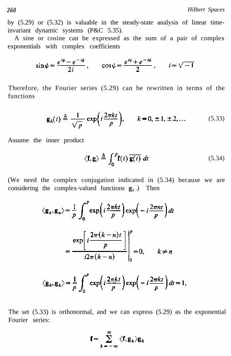
A sine or cosine can be expressed as the sum of a pair of complexexponentials with complex coefficients

Therefore, the Fourier series (5.29) can be rewritten in terms of thefunctions

(5.33)

Assume the inner product

(5.34)

(We need the complex conjugation indicated in (5.34) because we areconsidering the complex-valued functions gk .) Then

The set (5.33) is orthonormal, and we can express (5.29) as the exponentialFourier series:

f= ii (f&k,k==-ao


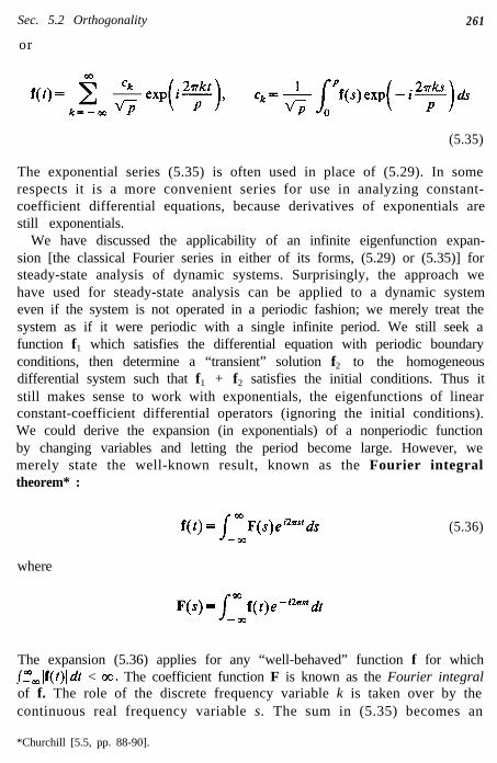
or

(5.35)

The exponential series (5.35) is often used in place of (5.29). In somerespects it is a more convenient series for use in analyzing constant-coefficient differential equations, because derivatives of exponentials arestill exponentials.

We have discussed the applicability of an infinite eigenfunction expan-sion [the classical Fourier series in either of its forms, (5.29) or (5.35)] forsteady-state analysis of dynamic systems. Surprisingly, the approach wehave used for steady-state analysis can be applied to a dynamic systemeven if the system is not operated in a periodic fashion; we merely treat thesystem as if it were periodic with a single infinite period. We still seek afunction f1 which satisfies the differential equation with periodic boundaryconditions, then determine a “transient” solution f2 to the homogeneousdifferential system such that f1 + f2 satisfies the initial conditions. Thus itstill makes sense to work with exponentials, the eigenfunctions of linearconstant-coefficient differential operators (ignoring the initial conditions).We could derive the expansion (in exponentials) of a nonperiodic functionby changing variables and letting the period become large. However, wemerely state the well-known result, known as the Fourier integraltheorem* :

f(t) = s O” F(s)e”“‘ds-00

(5.36)

where

F(s)=/m f(t)e-l’wstdt-00

The expansion (5.36) applies for any “well-behaved” function f for whichj_“,lf(t)ldt < cc. The coefficient function F is known as the Fourier integralof f. The role of the discrete frequency variable k is taken over by thecontinuous real frequency variable s. The sum in (5.35) becomes an

*Churchill [5.5, pp. 88-90].

262 Hilbert Spaces

integral in (5.36). Let q(s, t) A exp(i2mt). Then defining the inner product

by

Kg) A j-” f(t) g(t) dt-09

we can express (5.36) as

f(t) = /-O” (f, q(s, -)>n(s, t) ds-co

(5.37)

(5.38)

It can be shown, by a limiting argument, that the infinite set {q(s, e), - 00<s < cc} is an orthogonal set; however, Ilq(s, .)[I is not finite. Parseval’stheorem, a handy tool in connection with Fourier integrals, states that

(5.39)

where F and G are the Fourier integrals of f and g, respectively. Thisequation is a direct extension of (5.27). In effect, the “frequency domain”functions F and G constitute the coordinates of the “time domain”functions f and g, respectively. Equations analogous to (5.39) can bewritten for the expansions (5.29) and (5.35).

It is interesting that restricting our concern to periodic functions (or, ineffect, to the values of functions on the finite time interval [0,p ]) reduces(5.36) to (5.35) and allows us to expand these functions in terms of acountable basis (a basis whose members can be numbered using onlyinteger subscripts). Because of the duality exhibited in (5.36) and (5.39)between the time variable t and the frequency variable s, it should come asno surprise that restricting our interest to functions with finite“bandwidth” (functions whose transforms are nonzero only over a finitefrequency interval) again allows us to expand the functions in terms of acountable basis. Limited bandwidth functions are fundamental to theanalysis of periodic sampling. If F(s) = 0 for IsI > w, we say that f is bandlimited to w; or f has no frequency components as high as w. For such afunction it is well known that the set of samples (values) of f at the pointst = k /2w, k = 0, ±1, ±2,… contains all the information possessed by f. Tobe more specific, the sampling theorem states

(5.40)

for any function f which is band limited to w [5.18].

Sec. 5.2 Orthogonality 2 6 3

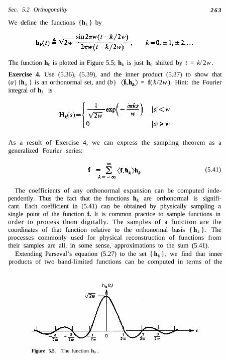
We define the functions {hk } by

The function h0 is plotted in Figure 5.5; hk is just h0 shifted by t = k/ 2w .

Exercise 4. Use (5.36), (5.39), and the inner product (5.37) to show that(a ) {h k } is an orthonormal set, and (b ) = f( k /2w ). Hint: the Fourierintegral of hk is

As a result of Exercise 4, we can express the sampling theorem as ageneralized Fourier series:

f = iit (f,h,)h,k=-co

(5.41)

The coefficients of any orthonormal expansion can be computed inde-pendently. Thus the fact that the functions hk are orthonormal is signifi-cant. Each coefficient in (5.41) can be obtained by physically sampling asingle point of the function f. It is common practice to sample functions inorder to process them digitally. The samples of a function are thecoordinates of that function relative to the orthonormal basis { hk }. Theprocesses commonly used for physical reconstruction of functions fromtheir samples are all, in some sense, approximations to the sum (5.41).

Extending Parseval’s equation (5.27) to the set { hk }, we find that innerproducts of two band-limited functions can be computed in terms of the

Figure 5.5. The function h0 .

264 Hilbert Spaces

samples of the functions:

(5.42)

If a function is both periodic and of finite bandwidth, then its Fourierseries expansion, (5.29) or (5.35), contains only a finite number of terms;periodicity guarantees that discrete frequencies are sufficient to representthe function, whereas limiting the bandwidth to less than w guarantees thatno (discrete) frequencies higher than w are required. Then, although (5.35)and (5.40) express the same function in different coordinates, the first setof coordinates is more efficient in the sense that it converges exactly in afinite number of terms. All the function samples are required in order toreconstruct the full function using (5.40). Yet (5.40) is dominated by itsfirst few terms; only a “few” samples are required to accurately reconstructthe function over its first period. The remaining samples contain littleadditional information.

Exercise 5. Let f(t) = sin2?rt, a function which is periodic and bandlimited. (F(s) = 0 for Is] > 1). Sample f at t = 0, + b, + 4, k :, … (i.e., letw = 2). Then, by (5.40),

The samples are zero for k = 0, ±2, ±4,. . . . Graphically combine the termsfor k = ±1, ±3, ±5, and compare the sum with f over the interval [0, 1].

5.3 Infinite-Dimensional Spaces

We developed the generalized Fourier series expansion (5.17) only forfinite-dimensional spaces; yet we immediately recognized its extension tocertain well-known infinite-dimensional examples, particularly (5.29). Ourgoal, ultimately, is to determine how to find orthonormal bases of eigen-functions for linear operators on infinite-dimensional spaces. A basis ofeigenfunctions permits decomposition of an infinite-dimensional operatorequation into a set of independent scalar equations, just as in the finite-dimensional case (5.23). Orthogonality of the basis allows independentcomputation of the coefficients in the expansion as in (5.24). We will findthis computational independence particularly valuable for infinite-dimensional problems because the “first few” terms in an infinite

Sec. 5.3 Infinite-Dimensional Spaces 265

orthonormal expansion dominate that expansion; we can ignore the re-maining terms.

To this point, wherever we have introduced infinite expansions ofvectors, we have used well-known examples and avoided discussion of themeaning of an infinite sum. Thus we interpret the Taylor series expansion

(5.43)

of an infinitely differentiable function f as the expansion of f in terms ofthe “basis” {1, t, t2, … }. We consider the Fourier series expansion (5.29) asthe expansion of a periodic function on the “orthonormal basis”

Yet the definition of linear combination does not pinpoint the meaning of2:”kmlckf, for an infinite set of functions {f k }. It seems natural anddesirable to assume that such an infinite sum implies pointwise conver-gence of the partial sums. Certainly, the Taylor series (5.43) means that foreach t,

as k+ cc. However, it is well-known that the sequence of partial sums inthe Fourier series expansion (5.29) of a discontinuous function is notpointwise convergent; the partial sums converge to the midpoints of anydiscontinuities (P&C 5.18). In an engineering sense, we do not care towhich value the series converges at a discontinuity. The actual value of thefunction is usually defined arbitrarily at that point anyway. We defineconvergence of the partial sums in a way which ignores the value of theFourier series at the discontinuities.

Convergence in Norm

Define y,, A 2’k = ~c~x~, the nth partial sum of the series z p= ickxk. We canassign meaning to the infinite sum only if the partial sums yn and ym

become more nearly alike in some sense as The natural defini-tion of “likeness” in an inner product space is likeness in norm. That is, y n

and ym are alike if the norm 11 y, - y, 11 of their difference is small. Aninfinite sequence {yn } from an inner product space ‘v is called a Cauchy

266 Hilbert Spaces

sequence if l]y,, - y, ]I-+0 as n, m+ cc; or, rigorously, if for each E > 0 thereis an N such that n,m > N implies ]Jy, - y,(] < E. Intuitively, a Cauchysequence is a “convergent” sequence. By means of a Cauchy sequence wecan discuss the fact of convergence without explicit reference to the limitvector. We say an infinite sequence {yn} from an inner product space Vconverges in norm to the limit x if I]x - y, ]I +O as rz+ 00.

Exercise 1. Use the triangle inequality (P&C 5.4) to show that asequence from an inner product space Ir can converge in norm to a vectorx in V only if it is a Cauchy sequence.

Assume the partial sums of a series, y, b X$= ickxk, form a Cauchysequence; by the infinite sum X2= i k k,c x we mean the vector x to which thepartial sums converge in norm, We call x the limit in norm of the sequence{yn}. (Note that the limit of a Cauchy sequence need not be in V. Themathematics literature usually does not consider a sequence convergentunless the limit is in V.)

Let ‘v be some space of functions defined on [0,1] with the standardfunction space inner product. One of the properties of inner productsguarantees that f = 8 if l]f]l = 0. We have assumed previously that f = 8meant f(t) = 0 for all t in [0,1]. Suppose, however, that f is the discon-tinuous function shown in Figure 5.6. Observe that ]]fl] = 0, whereas f(t)#Oat t = 0, ½ or 1. Changing the value of a function at a few points does notchange its integral (or its norm). We are hard pressed to define any innerproduct for a space containing functions like the one in Figure 5.6 unlesswe ignore “slight” differences between functions.

We say f = g almost everywhere if f(t) = g(t) except at a finite number ofpoints.* For most practical purposes we can consider convergence in normto be pointwise convergence almost everywhere. (However, Bachman and

Figure 5.6. A nonzero function with zero norm.

*The definition ofnumber of points.

“almost everywhere” can be extended to except a countably infinite


Narici [5.2, p. 173] demonstrate that a sequence of functions can beconvergent in norm, yet not converge at all in a pointwise sense.) Conver-gence in norm is sometimes called convergence in the mean. Convergencein norm is precisely the type of convergence which we need for discussionof Fourier series like (5.29). If f is a periodic function with period p, theFourier series expansion (5.29) means

(5.44)

That is, the sequence of partial sums converges in norm to the periodicfunction f. The convergence is pointwise almost everywhere-pointwiseexcept at discontinuities. It makes little practical difference how a functionis defined at a finite number of points. Therefore we usually do notdistinguish between functions which are equal almost everywhere. Ofcourse, our focus on the convergence in norm of a series of functions doesnot preclude the possibility that the convergence is actually pointwise and,in fact, uniform.

Infinite-Dimensional Bases

We need to extend the n-dimensional concept of a basis to infinite-dimensional spaces. We naturally think in terms of extending a finite sumto an infinite sum. An infinite set is said to be countable if its elements canbe numbered using only integer subscripts. We restrict ourselves to adiscussion of inner product spaces which have countable bases.*

Definition. Let ‘v be an infinite-dimensional inner product space. Let

5% A {x1, x2 ,…} be a countable set in ?‘“. Then % is said to be a basis forV if every vector x in V can be expressed uniquely as a convergentinfinite series x=~~Sickxk; that is, if there is a unique set of coordinates{c k} such that I]x- xz= ickxk]] can be made arbitrarily small by takingenough terms in the expansion.

Example 1. Bases for 9 (a,b). We denote by 9 (a, b) the infinite-dimensionalspace of all real polynomial functions defined on [a,b]. Since every polynomial is a(finite) linear combination of functions from the linearly independent set

9; {tk, k = 0,1,2,…}, F is a basis for 9 (a, b). Observe that no norm is needed todefine a basis for this particular infinite-dimensional space because no infinitesums are required. If we define an inner product on 9 (a, b), we can apply the

*A space which has a countable basis is said to be separable. Someuncountable bases. See Bachman and Narici [5.2, p. 143] for an example.

spaces have only

268 Hilbert Spaces

Gram-Schmidt procedure to the set 9, and generate a basis for 9 (a, b) consistingof orthogonal polynomials. (See, for instance, the Legendre polynomials of Ex-ample 2, Section 5.2.) Each vector in 9 (a,b) is a finite linear combination of theseorthogonal polynomials. Each different inner product leads to a different ortho-gonal basis. Of course, each such basis could also be normalized.

Any function that can be expanded in a Taylor series about the origin,as in (5.43), can be represented uniquely by the simple polynomial basis ofExample 1. Many familiar functions (et, sin t, rational functions, etc.) canbe expanded in such a series. These functions are not in 9 (a, b), and trueinfinite sums are required. Thus 3 appears to serve as a basis for spaceslarger than ‘Z? (a , b). How do we tell whether or not ‘% is a basis for anyparticular space Ir of functions? Of course, the coordinates of the functioncannot be unique without independence of the basis vectors. Our previousconcept of linear independence, which is based on addition and scalarmultiplication, applies only to finite-dimensional spaces. We say an infiniteset of vectors 5% is linearly independent if each finite subset of % islinearly independent. The vectors in a basis % must also span V in thesense that every x in ‘V must be representable. But, merely making % asufficiently large linearly independent set is not sufficient to guarantee that% is a basis. The set % of Example 1 is an infinite linearly independentset. Yet % is not a basis even for the “nice” space C?“( - 1,l) of infinitelydifferentiable functions. For example, if we define the functionf(t) A exp(-l/t2) to have the value f(0) = 0 at the origin, it is infinitelydifferentiable; but it has the Taylor coefficients f(0) = f’(0) = f”(O)/2 = …= 0. Thus an attempted Taylor series expansion of f converges to thewrong (zero) function.

According to a famous theorem of Weierstrass [5.4], any function int?(a,b) can be represented arbitrarily closely in a pointwise sense (and innorm) by a polynomial. Yet this fact does not imply that 9 is a basis forC? (a,b). We must still determine whether or not every f in C? (a, b) isrepresentable by a unique convergent expansion of the form ~~=&tk. Ingeneral, even though {xk } is an infinite linearly independent set, there maybe no approximation Xi= ickxk that will approach a given vector x in normunless the coefficients {c k} are modified as n increases. (See Naylor andSell [5.17], pp. 315-316.) It is difficult to tell if a specific set is a basiswithout displaying and examining the coordinates of a general vector inthe space. We will find that orthogonality of the vectors in a set easesconsiderably the task of determining whether or not the set is a basis.

Orthogonal Bases for Infinite-Dimensional Spaces

Actual determination of the coordinates of a specific vector relative to anarbitrary basis is not generally feasible in an infinite-dimensional space. It


requires solving for the numbers ck in the vector equation x = XT- ickxk; ineffect, we must solve an infinite set of simultaneous equations. However, ifthe basis !‘X is orthogonal (or orthonormal), the coordinates ck are theFourier coefficients, which can be computed independently. This fact isone reason why we work almost exclusively with orthogonal (or

orthonormal) bases in infinite-dimensional spaces. If ‘2% A {xk} is a count-able orthogonal basis for an inner product space Y, the Fourier seriesexpansion of a vector x in ‘v can be developed by an extension of theprocess used to obtain the finite-dimensional expansion (5.16)-(5.17). Letx j be one of the first n vectors in the infinite dimensional basis 3,. Let ci

be the ith coordinate of x relative to 3,. The Cauchy-Schwartz inequality*shows that

The right side of this expression approaches zero as n+oc. Therefore, foreach j < n,

as n+oo. Since the quantity approaching zero is independent of n, it mustequal zero, and

Thus the Fourier series expansion of x is

(5.45)

(5.46)

Of course, if the basis is orthonormal, the kth coefficient in (5.46) is justck = cx, xk)*

By an argument similar to the one above, we show that the coefficients{c k} in an orthogonal expansion are unique. Suppose x = zF= id&k is a

*P&C 5.4.

270 Hilbert Spaces

second expansion of x. Then by the triangle inequality,*

as n-+m. Then if x j is one of the vectors x1, …, xn, we again employ theCauchy-Schwartz inequality to find that as n+ 00

It follows that dj = cj, and the coordinates of x with respect to an ortho-gonal basis are unique.

Thus the only question of concern, if % is an orthogonal set, is whetheror not 5% is a large enough set to allow expansion of all vectors x in V. Ifthere is a vector x in V for which there is not a convergent expansion,then

is nonzero. Furthermore, z is orthogonal to each vector xj in 5% , and couldbe added to !X to make it more nearly complete (more nearly a basis).

Definition. We say an orthogonal set is complete in the inner product spaceV if there is no nonzero vector in V which is orthogonal to every vectorin 5%.

It follows from the discussion above that an orthogonal set ‘5% is a basisfor v if and only if it is complete in V. Any orthogonal set in a separablespace ?r can be extended (by adding vectors) until it is complete in V. Apractical technique for testing an orthogonal set {xk} to see if it is a basisconsists in showing that the only vector orthogonal to each vector xk is thezero vector 8. If ‘% is an orthogonal basis for Ir, then only for x = 8 is ittrue that all the Fourier coefficients (x,~) are equal to zero. Thus this test

*P&C 5.4.


for completeness of the orthogonal set !?C is equivalent to a test for validityof the Fourier expansion (5.46) for each x in V.

Example 2. Orthogonal bases for t?(a,b). The Weierstrass approximationtheorem [5.4] guarantees that any continuous function can be approximatedarbitrarily closely in norm by a polynomial. We noted earlier that this fact is

insufficient to guarantee that the set 9 b {t k , k = 0,1,2,…} is a basis for C? (a,b).

On the other hand, suppose that 8 2 { pk} is a basis for C? (a, b) consisting in realpolynomials pk which are orthogonal relative to some inner product. (We couldobtain 9 from %7 by the Gram-Schmidt procedure as in Example 2 of Section 5.2.)We now show that 8 is also a basis—an orthogonal basis—for C? (a,b). Let f be areal continuous function on [a,b]. Assume (f,p&= 0 for all polynomials pk in @ .We show that f must be the zero vector. By the Weierstrass theorem, for each e > 0there is a polynomial p, such that llf - pC(12 < C. Furthermore, since B is a basis forC? (a, b), p, = Cz= tckpk for some finite number N. Then

Since jlfl]‘+ jlp,112 < E for an arbitrarily small number l , llfl] = 0, and the function fmust be the zero vector. Thus the orthogonal set 9 is complete in 6? (a, b), and allorthogonal polynomial bases for ‘Z? (a,b) are bases for e (a,b) as well.

Harmuth [5.13] describes an interesting orthogonal basis for C! (a,b)—the set ofWalsh functions. These functions, which take on only the values 1 and -1, areextremely useful in digital signal processing; only additions and subtractions areneeded to compute the Fourier coefficients.

The classical Fourier series expansion (5.29) for periodic functions applies tofunctions f in the standard inner product space C?(a, b); we merely repeat thevalues of f on [a,b] periodically outside of [a,b] with period p = b - a. If we denotethe set of sinusoidal functions (5.30) by X, then the orthonormal set X iscomplete in C? (a,b ); it is an orthonormal basis for C? (a,b) .

Exercise 2. The Fourier series expansion (5.29) of a periodic function fcontains only sine terms if f is an odd function and only cosine terms if f isan even function. Show that in addition to the sine-cosine expansionmentioned in Example 2, a function in C?(O,b) can be expanded in twoadditional series of period p = 2b, one involving only sines (the Fourier sineseries), the other involving only cosines (the Fourier cosine series).

If {xk } is an orthonormal basis for v, the set of Fourier coefficients (orcoordinates) {(x, xk)} is equivalent to the vector x itself, and operations onx can be carried out in terms of operations on the Fourier coefficients. For

272 Hilbert Spaces

instance, we can compute inner products by means of Parseval’s equation:

bY)= / iit (x,x,>x,, 2 (&x,)x,\\k=I j-1

= 5 (X,Xk)(Y, x,)k-1

(5 .47)

(Because we are concerned primarily with real spaces, we usually drop thecomplex conjugate.) If y = x, (5.47) becomes Parseval's identity:

llxl12= 2 I(x,x,>12k-l

(5.48)

Equation (5.48) is also a special case of the Pythagorean theorem.Furthermore, it is the limiting case (equality) of Bessel’s inequality (P&C5.4). In point of fact, Bessel’s inequality becomes the identity (5.48) foreach x in ?I’- if and only if the orthonormal set {xk} is a basis for v.

Of course, not all bases for infinite-dimensional spaces are orthogonalbases. Naylor and Sell [5.17, p. 317] describe one set of conditions whichguarantees that a nonorthogonal countable set is a basis. However, rarelydo we encounter in practical analysis the use of a nonorthogonal basis foran infinite-dimensional space.

In a finite-dimensional space we can pick an inner product toorthonormalize any basis; specifically, we pick the inner product definedby Parseval’s equation (5.27). The infinite-dimensional equivalent (5.47) isless useful for this purpose because the unknown inner product is neededto find the coordinates in the equation. In an infinite-dimensional space,the choice of inner’ product still determines the orthonormality of a set ofvectors; but the norm associated with the inner product also determineswhether the vectors of an orthonormal set are complete in the space. Givena basis for an inner product space, what changes can we make in the innerproduct (in order to orthonormalize the basis) and still have a basis? Forspaces of functions defined on a finite interval, a positive reweighting ofthe inner product does not destroy convergence. For example, if {f k} is abasis for C?(a,b) with the standard function space inner product, then forany f in (?(a, b) (with unique coordinates {ck } relative to {f k}) and anye >O there is a number N such that Jb,lf(t)-Xi= 1C,f,(t)12dt < e for n > N.Suppose we define a new inner product for the same space of continuousfunctions:

(5.49)


where o(t) is bounded and positive for t in [a,b]. Then, using the samebasis {fk } and the same coefficients {c k},

where M is a positive bound on cc)(t). Since E is arbitrarily small, Me is alsoarbitrarily small. Thus for large enough n the partial sum is still arbitrarilyclose to f in the new norm. We represent by e(o; a,b ) the space ofcontinuous functions with the inner product (5.49). It is evident that thechoice of o affects the definition of orthogonality, but does not affect theconvergence or nonconvergence of sequences of vectors. Of course, theweighted inner product (5.49) does not represent all possible inner pro-ducts on the function space C? (a, 6); it does not allow for “cross products”analogous to those in (5.13). Yet it is general enough to allow us toorthogonalize many useful bases.

Example 3. Orthogonalizing a Basis by Weighting the Inner Product The shaftposition C/B of an armature-controlled motor as a function of armature voltage u isdescribed by

(J&(t) 4 !3$ + ep -u(t)

The eigenfunctions of L with the boundary conditions +(O) =+(b) = 0 are given by(4.38):

We pick the weight o in the inner product (5.49) so that the set {f k } is orthogonal:

for m # k. The functions {sin(lrkt/b)} form a well-known orthogonal basis for(Z (0, b ) using the standard function space inner product, as we noted in Example 2.Therefore, the weight o(t) = e’ makes the functions {f k} orthogonal with respect tothe weighted inner product. (The choice o(t) = 2e’/ b would make the setorthonormal. However, it is more convenient to normalize the eigenfunctions,multiplying each by w ).

274 Hilbert Spaces

We now demonstrate that the eigenfunctions {fk } are a basis [complete in6? (0, b )] by showing that the only function orthogonal to all functions in the set isthe zero function. Suppose (f, f,), = 0 for all k. Then

Since { sin( vrkt / b)} is an orthogonal basis with respect to the standard functionspace inner product, and since the Fourier coefficients of feti2 relative to this basisare all zero, fefi2 = 8 and f = 8. Therefore, {f k} is an orthogonal basis for the space6? ( e t; 0 , b). This orthogonal basis of eigenfunctions is used in Example 4, Section5.5 to diagonalize and solve the differential equation described above.

Hilbert Spaces

From Example 2 it is evident that a single infinite set can be a basis forseveral different infinite-dimensional spaces. Suppose {x k } is anorthonormal basis for an infinite-dimensional inner product space v.Presumably there are vectors x, not in V, which can be expanded uniquelyin terms of {xk} (assuming we extend the inner product space operationsto the additional vectors). What is the largest, most inclusive space forwhich {xk} is a basis? We refer to the largest space X of vectors whichcan be represented in the form of x = XT=, ckxk as the space spanned (orgenerated) by the basis {xk}. (Because {x k} is orthonormal, the coefficientsin the expansion of x are necessarily unique.) We show that X is preciselythe space of vectors x which are square-summable combinations of thebasis vectors; that is, x such that x = X2= i ckxk with Xr= i 1 ck12 < 00.

Suppose a vector x in X can be expressed as x =ZT. i ckxk, where {xk }is an orthonormal basis for the inner product space ‘v. Define

y, f X23., ckxk. Then {yn , n = 1,2, …} is a Cauchy sequence whichapproaches x, and jly, - yn(l+O as m, n+cc. If we assume n > m and usethe orthonormality of {x~}, we find (Iyn-ym(12= I~~~-,c,x,-~~,,c,x,~~~= 11X:=,+ 1c~~k(12=X~=m+ i Ic,J’. Therefore, Xi,n,+, (ck12-+0 as m, n--+00.It follows that Cz=,+ i Ick12-+0 as m-co; in other words, for each l > 0there is a positive number M such that m > M implies Xr-,,,+, 1 ck12 < e.Pick a value of E, and let m be a finite number greater than M. Then

Consequently, ZZ ?a i I ck I’ < cc, and x can be expanded on the basis {xk }only if x is a square-summable combination of the basis vectors. Con-versely, square summability of the coefficients {c k} implies that Ily, - y, (1’


-+O as m, n+co, and the sequence {y n} is a Cauchy (convergent) sequence.Thus any square-summable combination of {x k } must converge to somevector x in the space which we have denoted X.

It is apparent that X may be more complete than ‘V. If we were toassociate a single inner product space with the basis {xk }, the naturalchoice would be the largest space for which {xk } is a basis, the space x . IfV# X, then ‘V and X differ only in their “limit vectors.” Suppose xsatisfies x = ET=, ckxk, and again denote the nth partial sum by ynZ-pk- i ckxk. The sequence of partial sums {yn } is a Cauchy sequence withlimit x. Thus each x in X is the limit of a Cauchy sequence in V. In pointof fact, X differs from V only in that X contains the limits of moreCauchy sequences from Ir than does li‘.

Example 4. A Cauchy Sequence in (? (0,l) with no Limit in e(O, 1). The func-tions { f k } of Figure 5.7 form a Cauchy sequence in e(O, 1) with the standardfunction space inner product (5.16); that is,

s‘(t(t)-fJt))‘dt+O as n,m+w

0

The limit in norm of the sequence {f k } is the discontinuous function

f(t)= 1, t<f

0, t>+

which is not in L? (0,1). The limit vector f is a member of a space which is largerand more complete than e(O, 1). Yet f can be expanded uniquely in the sine-cosine basis (5.30) for e(O, 1).

Definition. Let S be set in an inner product space ?r. A vector x in ‘V iscalled a point of closure of S if for each E > 0 there is a vector y in S such

Figure 5.7. A Cauchy sequence in i? (0,l).

276 Hilbert Spaces

that 11x- yll < E; that is, x can be approximated arbitrarily closely in normby vectors y in S . The closure of S , denoted 5, consists in S togetherwith all its points of closure. If $5 contains all its points of closure, it is saidto be closed. A set S, in S is said to be dense in S if S is the closure ofS,; that is, if every vector in S can be approximated arbitrarily closely innorm by a vector in S 1.

Definition. An inner product space X is said to be complete if everyCauchy (convergent) sequence from X converges in norm to a limit in X .A complete inner product space is called a Hilbert space.

The terms closed and complete, as applied to inner product spaces, areessentially equivalent concepts. The inner product space V discussedabove is not complete, whereas the “enlarged” space X is complete; x isa Hilbert space. The space ‘v is dense in X; that is, X is only a slightenlargement of V. We can complete any inner product space by extendingits definition to include all of its limit vectors. Of course, the definitions ofaddition, scalar multiplication, and inner product must be extended tothese additional limit vectors [5.11, p. 17].

Example 5. Finite-Dimensional Hilbert Spaces. Every finite-dimensional innerproduct space is complete [5.23, p. 143]. For instance, we cannot conceive of aninfinite sequence of real n-tuples converging to anything but another real n-tuple;the ith components of a sequence of n-tuples constitute a sequence of real numbers,and the real numbers are complete.

Example 6. The Hilbert Space 1,. We denote by li the space of square-summable

sequences of complex numbers with the inner product (x, y) A IX?=, &qkjk, where 5;,and Q are the kth elements of x and y, respectively. (A square-summable sequenceis a sequence for which llx112=200k= 1 l&l2 < oo .) We use the symbol l2 to representthe space of real square-summable sequences; then the complex conjugate in theinner product is superfluous. Both the real l2 and the complex 1; are complete [5.23,p. 48]. The standard basis {Ed}, where ej = (0, . . . , 0, li, 0, . . . ), is an orthonormal basisfor both the real and complex cases.

Example 7. The Hilbert Space C,(a,b). Let C$ (a,b ) be the space of complexsquare-integrable* functions defined on the finite interval [a,b] with the inner

product (f,g) A $if(t)g(t)dt. (A square-integrable function is one for whichllfJ12= Jf: If(t)l”dt is finite.) The symbol $(a,b) is used to represent the space ofreal square-integrable functions; then the complex conjugate is unnecessary. Weusually concern ourselves only with the real space. Both the real E,(a,b) and thecomplex g (a,b) are complete [5.2, p. 115]. The space k?,(a,b) contains no deltafunctions. However, it does contain certain discontinuous functions, for example,

*The integral used in this definition is the Lebesgue integral. For all practical purposes, wecan consider Lebesgue integration to be the same as the usual Riemann integration. Wherethe Riemann integral exists, the two integrals are equal. See Royden [5.21].


step functions. (Recall from the definition of equality in norm that we ignoreisolated discontinuities. As a practical matter, we seldom encounter a function withmore than a few discontinuities in a finite interval.) We can think of C,(a,b) asessentially a space of functions which are piecewise continuous, but perhaps

unbounded, in the finite interval [a,b]. Any set 9 A {pk } of orthogonal poly-nomials which forms a basis for CP (a,b ) is a basis for both the real and complexE*(a,b). An orthonormal basis for both the real and complex !Z,(a, 6) is the set ofsinusoids (5.30), with p = b - a. Another orthonormal basis for the complex C$ (a, 6)is the set of complex exponentials (5.33) with p = b - a.

Example 8. The Hilbert Space C,(w; u, 6). Let C2(w; a , b) represent the set of all-square-integrable functions with the inner product (5.49). That is, h(w;

contains those functions that have finite norm under the inner product (5.49).From the discussion associated with (5.49) it is apparent that lZZ(w; a,b) differsfrom e2(a, b) only in the inner product. Both spaces contain precisely the samefunctions, and completeness of h(w; a,b ) follows from the completeness ofMa, b).

A Hilbert space possesses many subsets that are themselves innerproduct spaces (using the same inner product). These subsets may or maynot be complete. If a subset is a complete inner product space, it is itself aHilbert space, and we refer to it as a subspace. If a subset is a vector space,but is not necessarily complete, it is properly termed a linear manifold.Since all finite-dimensional vector spaces are complete, all finite-dimensional linear manifolds of Cz(a, b) are subspaces. However,

and the space of piecewise-continuous func-tions on [a , b] are (incomplete) linear manifolds of F2(a, b). Each of thesespaces is dense in &(a, b), and thus is nearly equal to &(a, b).

We note that if X is a Hilbert space and S is any set in X, then theorthogonal complement S L must be a subspace. For if {xn } is a Cauchysequence in SL with limit x in X, then (x,, y) = 0 for each y in S ; itfollows that

and the limit vector x is also orthogonal to S . [In order to take the limitoutside the inner product, we have relied on the continuity of innerproducts. See (5.56).]

Example 9. An Infinite-Dimensional (Complete) Subspace of &(a,b). Let ‘?lS bethe (one-dimensional) subspace of constant functions in C,(a, b). By the previousparagraph, the orthogonal complement %I is complete. But w1 consists in thosefunctions f in f&(a, 6) which satisfy = 0 for all constants c. Thus thefunctions in %(a, b) whose average value is zero form a complete subspace of!Qa, b). This subspace is itself a Hilbert space.

278 HiIbert Spaces

Why do we care whether or not a vector space is complete? One reasonis that we wish to extend finite-dimensional concepts to infinite-dimensional cases. Some of these concepts extend only for a Hilbert space,the natural generalization of a finite-dimensional space. (Recall that finite-dimensional spaces are Hilbert spaces.) The only concept we have dis-cussed thus far which applies only for Hilbert spaces is the projectiontheorem (5.20), V = % 63 %I. The proof of (5.20) depends on the factthat repeated application of the Gram-Schmidt procedure can generate nomore than n orthogonal vectors in an n-dimensional space. The theorem isvalid in an infinite-dimensional space V if and only if ‘V is a Hilbertspace and % is a (complete) subspace of [5.2, p. 172]; of course, %l isalways complete.

Fortunately, the question of completeness of an inner product space isseldom of practical concern, since we can complete any inner productspace by extending its definition. Suppose a linear transformation T has itsdomain and range in a separable Hilbert space X (a Hilbert space with acountable basis). Then if domain(T) is dense in X, we refer to T as alinear operator on the Hilbert space X . For instance, the completion of thespace (?“(a, b) of real, infinitely differentiable functions on [a,b] is justf&(a,b) of Example 7. We apply a differential operator L to any space of“sufficiently differentiable” functions and still refer to L as a differentialoperator on e2(a, b).

In our examination of finite-dimensional vector spaces we used theprocess of taking coordinates to equate every n-dimensional space to thematrix space w x ‘. We now equate inner product spaces, both finite andinfinite-dimensional. Two inner product spaces, V with inner product( , )y and % with inner product ( , )w, are isomorphic (or equivalent)if there is an invertible linear transformation T: ?/+qti which preservesinner products; that is, for which (x,Y)~ = (Tx,Ty), for all x and y inV. The process of taking coordinates relative to any orthonormal basis isjust such a transformation.

Example 10. Coordinates for Real n-Dimensional Inner Product Spaces. For n-dimensional spaces, we take 91Lnx 1 with its standard inner product as our space ofcoordinates. Let Ir be any real n-dimensional inner product space; let !X be anorthonormal basis for ?r, Define T: ‘Y+ 9Rn x ’ as the invertible linear transforma-tion which assigns to each vector x in ‘v its set of Fourier coefficients (orcoordinates) in 9L’ x ’ :

TX A ((x,xJy * * * <Jv%JY)‘= b&x

Since % is orthonormal, Parseval’s equation (5.27) is satisfied:

Sec. 5.4 Adjoint Transformations 279

This is the standard inner product in the real space ‘3Lnx ‘. Clearly, each realn -dimensional inner product space (a Hilbert space) is equivalent to 9Rnx ’ with itsstandard inner product. (By inserting a complex conjugate in the inner product, wecan show that every complex n-dimensional inner product space is equivalent to9R z x ‘, the space of complex n x 1 matrices with its standard inner product.)

Example 11. Coordinates for Real Separable Infinite-Dimensional Hilbert Spaces.The logic of Example 10 applies to all separable Hilbert spaces (Hilbert spaceswhich have countable bases). For separable infinite-dimensional spaces, we take 1,with its standard inner product as our space of coordinates. A separable space hasa countable basis. Any such basis can be orthonormalized by the Gram-Schmidtprocedure. Suppose !!X = {xk } is an orthonormal basis for a real separable Hilbertspace X. We define T: X+Z, as the process of assigning Fourier coefficientsrelative to this basis :

TX b ~x,~~c,<x~x~)~c, . ..)=bdn (5.50)

From our discussion of the space spanned by an orthonormal basis, we know thatthe coordinates (Fourier coefficients) of vectors in X consist in the square-summable sequences which constitute Z,. Since Fourier expansions exist and areunique for each x in 3c, T is invertible. Because the set {xk } is orthonormal,Parseval’s equation (5.47) applies:

This is the standard inner product between the coordinates of x and y (in /,).Therefore, every real separable infinite-dimensional Hilbert space is equivalent tothe real space Z, with its standard inner product. Thus the somewhat mysteriousspace lQa, b) is, in essence, no more complicated than Z2. In Example 11 of Section5.4 we introduce IQQ), an inner product space of square-integrable functionsdefined on a finite two-dimensional domain a; lZ,(Q) is also equivalent to Z,. (Byinserting a complex conjugate in each inner product, we find that every complexseparable infinite-dimensional Hilbert space is equivalent to the complex space 1;with its standard inner product.)

5.4 Adjoint Transformations

In the preceding section we developed separable Hilbert spaces as naturalgeneralizations of n-dimensional inner product spaces. We know that wecan generate a countable orthonormal basis for any such space. In (5.25)we diagonalized and computationally decoupled an operator equation inan n-dimensional space by means of an orthonormal basis of eigenvectors.We have also discussed the applicability of orthonormal eigenvectors to aninfinite-dimensional example, the steady-state analysis of a dynamic sys-

280 Hilbert Spaces

tem. Can we diagonalize a general linear operator on an infinite-dimensional space, a differential operator, for instance? We can if there isa countable orthonormal basis for the infinite-dimensional space which iscomposed of eigenvectors of the operator. In Example 3, Section 5.3 weorthogonalized a set of eigenfunctions by careful choice of the innerproduct. We would like to be able to make general statements whichclearly characterize the existence of an orthonormal basis of eigenvectorsfor a given operator on a given infinite-dimensional space. Given a set ofeigenvectors for an operator T on a given vector space ?r, for what innerproducts are the eigenvectors an orthogonal (or orthonormal) basis? Forwhat operators T on a given inner product space ‘V do there existorthonormal bases of eigenvectors? In sum, under what conditions can wediagonalize an operator equation by means of an orthonormal basis? Theanswers to these questions are to a great extent answered in the concept of“self-adjointness.” We introduce the adjoint transformation in this section,and return to a discussion of orthonormal bases of eigenvectors for solvingoperator equations in Section 5.5.

We observed in Chapter 1 that we can interpret a matrix multiplicationAx either as a linear combination of the columns of A or as a set ofstandard inner products of x with the rows of A. Furthermore, we knowthat the number of independent rows of A equals the number of indepen-dent columns. Since the rows and columns of A possess much commoninformation, we would be surprised if multiplication by the transposedmatrix AT did not describe a transformation closely related to multiplica-tion by A. Let T: %2x ‘-+ %3x ’ be defined by

We define the “transpose” transformation TT: ‘?%3x ‘+ %2x ’ by

TTyAATy=(; ; ;)y

The range and nullspace of T are important indicators of its structure.of theThey display the nonsolvability and nonuniqueness of solutions

equation Tx = y. Observe that

range(T) = span , nullspace(T ) = span

range(T T) = span nullspace(T T) = span


Range(T) and nullspace(T ) are, of course, in different spaces. However,range(T ) and nullspace(T T) are in the same space; in fact,

9.,3x ’ = r a n g e (T) nullspace(T T)

Similarly,

Gsrc2x ’ = r a n g e (T T) nullspace(T)

Furthermore, these direct sums are orthogonal relative to the standardinner products for the two spaces. It is evident, at least for this example,that T and TT together characterize the transformation T more explicitlythan does T alone.

We extend the transpose concept to general linear transformations. Wefind that the orthogonal decomposition illustrated above still applies.Recall that orthogonal decomposition is closely related to Fourier seriesexpansion and, therefore, to orthonormal bases. The generalization of TT,together with T itself, characterizes the existence or nonexistence oforthonormal bases of eigenvectors.

Bounded Linear Transformations

The generalization of the transpose matrix exists only for transformationswhich satisfy certain restrictions. We now define the concepts which weuse to express these restrictions.

Definition. Let T be a (possibly nonlinear) transformation from an innerproduct space ?‘- into an inner product space ‘?6. Then T is bounded ifthere is a positive number a such that

IIWl~ 6 4lxll Y for all x in Ir (5.51)

We define the norm of T by*

IlTil 2 inf{ a: IITxlJ w Q allxll y for all x in v} (5.52)

We can think of lITI as the tightest bound for T. It follows that

IITXII w Q IITII llxll Y (5.53)

*The term "inf” means infimum or greatest lower bound. If the bound is actually reached, theinfimum is just the minimum. The term “sup” means supremum or least upper bound; if thebound is attained, the supremum is the maximum.

282

If T is linear, (5.52) can be expressed as

IlTll =infi

II WI wct:ll~lly Gcx

1

=inf{lx:JITxll, < LY, IIxllv=l}

= SUPII,IIv= I{ IIWI 9lf >

Hilbert Spaces

(5.54)

Example 1. A Norm is a Bounded Functional. Define T: Ir+% by Tx b llxllV.Then IITx/I~ = lTxl= IlxllV. Clearly, the number 1 is a bound for T and llTl1 = 1.

Example 2. Matrix Transformations are Bounded. Define T: 9Rzx l+ 9R~” ’ by

Tx 4 Ax, where A is a (possibly complex) m x n matrix. Assuming standard innerproducts, llTxl12 = JlAx112 =-T-Tx A Ax. Then, by (5.54), IlTl12=maxxTxI iXTATAx. It canbe shown that lITI = a , where &,, is the largest eigenvalue of the matrix A’A(see P&C 5.29). We call K the spectral radius of A and denote it by a(A). Wealso refer to a(A) as the norm of A, denoted [[All. Thus

IITII = llAll= b(A) = a

It is apparent that the bound a is attained for x equal to a normalizedeigenvector of xTA corresponding to the eigenvalue A,. The fact that matrixtransformations are bounded implies that all transformations on finite-dimensionalspaces are bounded.

If A is square, it makes sense to speak of the eigenvalues of A itself. If A is alsoreal and symmetric, its spectral radius is just the largest eigenvalue of A. That thisstatement is not true for every square matrix is demonstrated by the matrix

for which the largest eigenvalue is A= 1, but for which llAll = a(A)= fi . Thebound [IA11 is attained for x = (1 1)T.

Example 3. Integral Operators are Bounded Define the linear operator T onC,(a,b) by (Tf)(t)= Jik(t,s)f(s)ris, where the kernel k satisfies 12 1: k2(t,s)drdt< cc. Such a kernel is called a Hilbert-Schmidt kernel and T is known as aHilbert-Schmidt integral operator. If k is bounded for t and s in [a , b], for instance,then T is Hilbert-Schmidt. Many operators are of this type; for example, theinverses of most differential operators defined on a finite interval. We apply the


Cauchy-Schwartz inequality (P&C 5.4) to find

Therefore, by (5.54),

(5.55)

and T is bounded. Under what conditions is the bound (5.55) actually the norm ofT ? The Cauchy-Schwartz inequality becomes an equality if and only if the twoarguments k(t,s) and f(s) are dependent functions of s. Therefore, if there is an f inC2(a, b) such that k(t,s) = g(t)f(s), then the bound which we have exhibited isactually llTl1. For many integral operators, IIT is equal to the magnitude of thelargest eigenvalue of T (P&C 5.29).

Example 4. Differential Operators are not Bounded Differential operators areamong the most useful transformations, yet they are seldom bounded. For instance,let D operate on C2(0, 1). Let {fk } be the sequence of functions shown in Figure5.8a. In the & norm, llf11j2= l$‘dt = f and JJf,ll’= SAdt= 1. Therefore, thefunctions in the sequence satisfy

Ilf,l12= i < llf/cl12< 1 = llfall12

Yet we recognize from Figure 5.8b that

There is no number (Y which “bounds” D for all f in lZ2(0, 1). In the limit as k-w,an equivalent statement is that the derivative of a discontinuous function containsa delta function, but delta functions are not square integrable; they are not inMO, 0.

Definition. A (possibly nonlinear) transformation T: y--+ ‘?6 is said to becontinuous at x0 if for each E > 0 there is a 6 > 0 such that

284 Hilbert Spaces

Figure 5.8. Differentiation of a sequence of functions.

That is, T is continuous at x0 if making 11x - x,,ll y small will guarantee thatIlTx -Tqllw is small. If T is continuous for each x in ?‘-, we just say T iscontinuous.

The nonlinear transformation Tx A llxllV, for example, is continuous.

Suppose T is continuous and x0 = lim,,, xn in II. If xn approaches x0 ,then Txn approaches Tx0; in other words,

&I& (TX,,) = TX, = T( ;;l x,,) (5.56)

We will find this fact useful in the decoupling of equations on infinite-dimensional spaces. It is easy to show that a linear transformation iscontinuous if and only if it is bounded. Thus the linear transformations ofExamples 2 and 3 are continuous transformations. It is apparent thatbounded (or continuous) linear transformations are “well behaved.” Thelinear differential operators of Example 4 are not continuous and are


“poorly behaved.” It is for bounded (continuous) linear transformationsthat we will show most of the useful results of this chapter. It is usuallydifficult, if not impossible, to extend these concepts to unbounded lineartransformations in a rigorous manner. Yet the concepts will be shown, byexample, to extend in certain instances.

Completely Continuous Transformations

We now introduce briefly the concept of “complete continuity” of a lineartransformation in order to specify conditions which guarantee the exis-tence of a countable basis of eigenvectors.

Definition. A set S in an inner product space Ir is said to be bounded ifthere is a constant M such that llxlj < M for all x in 5 . A set S is compactif each infinite sequence of vectors from $ contains a subsequence thatconverges to a vector of S . Every compact set is closed and bounded. Infinite-dimensional spaces the converse is also true: a set is compact if andonly if it is closed and bounded, and every bounded set is closed [5.22, p.185].

It is easy to see that a linear transformation T: ‘v+% is bounded(continuous) if and only if it maps bounded sets in ‘V into bounded sets in?6. A stronger restriction on T, which guarantees the countability of theeigenvalues and eigenvectors of T, is that of complete continuity.

Definition. A linear transformationbounded sets into compact sets.

T is completely continuous if it maps

A completely continuous transformation is continuous, but the converseis not necessarily true. On an infinite-dimensional space, even the (con-tinuous) identity operator is not completely continuous. Any boundedlinear transformation whose range is finite-dimensional is completely con-tinuous; thus any operator on a finite-dimensional space is completelycontinuous. The Hilbert-Schmidt integral operators of Example 3 are alsocompletely continuous. Suppose T and U are completely continuoustransformations mapping 1/ into % ; then the linear combination aT + bUis completely continuous. If T and U are linear operators on V, one ofwhich is bounded and the other completely continuous, then TU and UTare completely continuous. If Tk is the kth member of a sequence ofcompletely continuous linear transformations mapping Ir into %, thenthe limit operator T defined by

k”“, llTk-Tll =0-3

is completely continuous. If a completely continuous transformation T is

286 Hilbert Spaces

defined on a infinite-dimensional space, then T-1, if it exists, is un-bounded. Detailed discussions of completely continuous transformationscan be found in Bachman and Narici [5.2] and Stakgold [5.22]. We contentourselves with this brief introduction; however, we make occasional re-ference to the consequences of complete continuity.

Bounded Linear Functionals

The key theorem in the development of a generalization of the transposematrix is the Riesz-Frechet theorem. This theorem relates inner productsand “bounded linear functionals.” As indicated in Section 2.3, a functionalis a scalar-valued transformation. Suppose ‘V is an inner product space.

The transformation B: V-+e defined by Bx A (x,Y)~ for a fixed vector yin V is a linear functional. (Recall that an inner product is linear on theleft.) By the Cauchy-Schwartz inequality (P&C 5.4), ]]Bx]le = I(x,~)~]

< IIYllvlla-v and l]yl]V is a bound for the linear functional B. Further-more, the bound is attained with the normalized vector x = y/]]yl] y, andthus l]Bl] = I]y]lV. Each different y in ‘v specifies a different bounded (orcontinuous) linear functional. If ‘Ir is a Hilbert space, we can say more—any bounded linear functional on Ir can be represented by an innerproduct.

Riesz-Fréchet Theorem. Corresponding to any bounded linear functionalB on a Hilbert space X there is a unique vector y in X such that

Bx=(x,~)~ for all x in x (5.57)

Furthermore, l]B]] = l]yllx.

Proof. If B is the zero functional, it is obvious that y = 0. Assume B is notthe zero functional, and let ‘?!ti = nullspace(B ). (% consists of all x in ‘Xfor which Bx = (x, y> = 0. Thus the vector y which we seek spans %I.) Lety0 be a unit vector in %‘-, and x any vector in X . The vector (Bx)y0 -(By0 )x is in % (verified by substitution into Bx = 0).* Therefore,

((Bx)y, - (By& Y,-,> = (Bx) - (BY& Yo) = o

or Bx = (x, (By,)y,,). The vector y = (By,)y, in ‘?6* represents B as requiredby (5.57). To see that y is uniquely determined by B, we assume both y andz will do. Then (x, y) = (x,z> or (x, y -z) = 0 for all x in X including

*Since range(B ) is one-dimensional, Bx and By0 are scalars; they can be used as scalarmultipliers.


x = y - z. It follows that y - z = 8 or z = y. We showed that llBll= llyll y inthe discussion prior to the theorem.

Example 5. Bounded Linear Functionals on %T x1* Any linear functional B onthe standard inner product space 9lLz x ’ is bounded and representable as Bx =~TXfor some y in 9X$” ‘. That is, a linear functional acting on n X 1 matrices isnecessarily the taking of a specific linear combination of the n elements of thematrices. Furthermore, llBll= jlyll= m = u(y), the spectral radius of the n x 1matrix y.

Example 6. Bounded Linear Functionals on &(a,b). The most general bounded

linear functional B on the standard Hilbert space E,(a, b) is Bu A 1 i u(t)g( t)dt forsome specific g in Cz(a, b), and llBll= [ $ z Ig(t)12dt]‘/2. For example, the response fof a single-input linear time-invariant dynamic system with zero initial conditions isthe convolution of the system input u with the impulse response g* :

f(t)=loru(s)g(t-S)ds

For the interval 0 < t < b, this function can be written

f(t) = jobu(s)k,(s) ds = (u, k,)

where

k,(s)=g(t-s) s< t

=o s>t

Thus for each instant t, f(t) is a bounded linear functional on C,(O, 6). The functionin C,(O,b) that represents the linear functional is kt. Treated as a function of t ands, kt(s) is the Green’s function for the dynamic system (see Chapter 3). A crudemeasure of the effect of the linear functional is the norm of the functional,

Ilk~ll=[S~g2(t-s)~l”2.

Example 7. Function Evaluation, an Unbounded Linear Functional. Define B:

C2(a, b)+% by Bf b f(t0), where t0 is in [a , b]. This linear functional, evaluation att0, is not bounded. For if fk is a pulse of height k and width 1/k2, centered at t0,then llfkll= 1, but IlBf,II=k+co. It is well known that f(te)= $tf(t)i!S(t-to)&,where 6 (t - t0 ) is a Dirac delta function centered at t0 .† Thus in a sense theRiesz-Fréchet theorem extends to at least this unbounded linear functional. How-ever, 8 (t - t0 ) does not have a finite norm and therefore is not in !Z$(a, b).

*See Appendix 2 for a discussion of convolution and impulse response.† See Appendix 2 for an introduction to the properties of delta functions.

288 Hilbert Spaces

The Adjoint

Let T: V+ % be a bounded linear transformation between Hilbert spacesIr and %. We now introduce the adjoint transformation T*, a generaliza-tion of the transposed matrix multiplication with which we introduced thissection. The vector Tx is in %!. Since an inner product is a bounded linear

functional of its left argument, Ux A (Tx,z)% is a bounded linear func-tional of the variable x in V. In fact, by means of the Cauchy-Schwartzinequality (P&C 5.4) and the inequality (5.53), we can exhibit a bound:

IlUxll w = Iww>, I g IlWGzlr Il4lw < IITII ll4lvll4l~

or IlUll < lITIt llzll QJ - The Riesz-Fréchet theorem (5.57) guarantees thatthere exists a unique vector y in ‘V which represents this bounded linearfunctional U in the sense that

Ux= (TJw), = (x,Y)~

It is evident from this equation that y in V and z in w are related. Wedefine this relation to be the adjoint transformation, y = T*z.

Definition. The adjoint transformation T* is defined by

<TX, z>w = (x, T*z)~ (5.58)

for all x in V and z in %.The existence of T* is guaranteed by the bounded linear nature of T and

the completeness of V. Uniqueness and linearity of T* are easily verified.Furthermore, T* is bounded; we recognize that

IIT*zll Y = IIYII Y = IlUll G IITII llzll GUT

By (5.54),

Since (5.58) is symmetric in T and T*, reversing the roles of T and T*shows that lITI < llT*ll. Thus

IlTll = IF* II (5.59)

An explicit description of T* can be obtained from the defining equation(5.58) and a description of T. The basic technique for obtaining the


description of T* is to write (Tx,z), and manipulate it into the form of(~,T*z)~; in effect, we work operations off of x and onto z.

Example 8. The Adjoint of a Matrix Transformation. Let V = ERf” ’ and W

= Gsrcc”x1, each with its standard inner product. Define T: ‘v+% by Tx b Ax,where A is an m X n matrix. Then

(TX, z> q,r = (AT z> q~

= I’h

=(Az)=x

= (x,it=~)~ = (x, T*z),

Clearly,

T*z = AZ (5.60)

Of course, if A is real (or if Y and % are real) the conjugate is superfluous. It isapparent that the transposed matrix example with which we introduced Section 5.4is just a special case of the general adjoint concept. If the inner products are notstandard, multiplication by the conjugated transposed matrix is not the adjoint(P&C 5.19).

Example 9. The Adjoint of an Integral Operator. Let ‘v = W = F.$ (a,b). Define

T by (‘R)(t) h J 2 k(t,s)f(s)dr, where k is a Hilbert-Schmidt kernel; by Example 3,T is bounded. Then

Therefore,

@‘*g)(t) 4 Jbk(s,g(s)dsa

(5.61)

290 Hilbert Spaces

Whereas T requires integration with respect to the first variable in the kernel k, T*requires integration with respect to the second variable. The kernel k(s, t) is theanalogue of the conjugated transposed matrix of Example 8. Once again, if thespaces are real, the conjugations are superfluous.

Exercise 1. Let V = % = &(w; a , b ), for which the inner product is(5.49). Assume the scalars are real. Define T: V+% by

(Tf)(t) 2 jbk(t,s)f(s)dsa

where k is a Hilbert-Schmidt kernel. Show that

(5.62)

Adjoints of Differential Operators

Only for a bounded linear transformation on a Hilbert space does thepreceding discussion guarantee the existence of an adjoint transformationwhich satisfies (5.58) and (5.59). In point of fact, if T is not bounded, itmakes no sense to speak of lITI/. Yet among the most useful transforma-tions are the linear differential operators, which are unbounded. Thus ifthe adjoint concept is useful, we have reason to attempt to apply theconcept to differential operators. We shall see that differential operatorsdo have adjoints.

Consider the simple differential operator D defined by ( Df)( t ) g f’(t)acting on functions defined over the interval [a,b]. Assume the standardfunction space inner product for both the domain and range of definition.Nothing prevents us from using the approach of Examples 8 and 9 to try togenerate an adjoint for D. The natural technique for working differentia-tions off of one argument and onto another is integration by parts:

(Df,g)= j-br’(t)g(t)dta

= f(tk(t>lb, - Jbf(r)gYt)d~a

(5.63)

It seems logical to define D* by (D*g )(t) A -g’(t) = (-Dg)(t ). However,this definition does not quite agree with the defining equation (5.58) unlessthe boundary term, f(b) g (b) - f (a) g( ) ,a is zero. We must not lose sight of


the fact that differential operators usually have associated boundary condi-tions. Suppose the boundary condition associated with D is f (a ) - f( b) = 0.Then in order that the boundary term of (5.63) be zero, we must havef(b)[g (b) - g (a)] = 0, or g (b) - g (a) = 0.

It should be apparent that for any ordinary linear differential operator Lwith a set of accompanying homogeneous boundary conditions we can useintegration by parts to generate an adjoint differential operator L* withaccompanying adjoint homogeneous boundary conditions. The operatorsL and L* satisfy the defining equation, (5.58), for all f and g in &(a,b)which satisfy the respective boundary conditions. [Of course, we havegiven up on (5.59).] If we were to change the homogeneous boundaryconditions associated with L, we would obtain a different set of adjointboundary conditions, but the same adjoint differential operator L*. Werefer to the adjoint differential operator L* as the formal adjoint of L. Theformal adjoint is independent of boundary conditions. The definition of anoperator always includes a definition of its domain. We use the homo-geneous boundary conditions associated with L to restrict the domain of L.The adjoint boundary conditions, which arise naturally out of the integra-tion by parts, determine the restrictions on the domain of the formaladjoint L* in order that it be a true adjoint of L [in the sense that it obeys(5.58)]. Thus the formal adjoint of D is D* = -D. If the boundarycondition associated with D is an initial condition, f(a) = 0, then by (5.63)the adjoint boundary condition is a final condition which requires thatg(b) = 0 for each g in the domain of D*.

If we wished, we could further restrict the domains of L and L* toinclude only differentiable functions, thereby eliminating delta functionsand their derivatives from range(L) and range(L*). However, formal use ofintegration by parts works for delta functions. Therefore, as a practicalmatter, we do not concern ourselves with this restriction.

Example 10. The Adjoint of Dn . Let the nth derivative operator Dn act on a spaceof real functions defined over [a,b]. Assuming the standard inner product,

292 Hilbert Spaces

(The intermediate terms are indicated only to show the pattern which the termsfollow. Some of the terms shown are extraneous if n = 1 or 2.) The formal adjoint ofD n is clearly (-l)n D n. The adjoint boundary conditions depend upon theboundary conditions associated with Dn. A specific set of boundary conditionsdoes not determine a unique set of adjoint boundary conditions. However, thedomain defined by the adjoint boundary conditions is unique.

Exercise 2. Show that the formal adjoint of the differential operatorL&D”+qD”-‘+... + a,1 acting on a space of functions with the stan-

dard inner product is L* ~(-l)“D”+(-l)“-‘a,D”-‘+*** +a,$

Example 11. The Adjoint of a Partial Differential Operator. Let e,(8) be thespace of real functions which are defined on a two-dimensional region Q and whichhave finite norm under the inner product

(f, g} A /,f(P)dP) dP (5.64)

where p = (s , t ), an arbitrary point in !k We define the Laplacian operator V2 on

f%) by

for (s,t) in 52

For this problem, the symmetric form of Green’s theorem is the equivalent ofintegration by parts; it states

(5.65)

where r represents the boundary of the region St, and the subscript n indicates thederivative in a direction normal to r and directed out of 8.* Using this theorem,we find

Clearly, the formal adjoint of V2 is just V2 itself.Not all boundary conditions are appropriate for a partial differential operator.

For the Laplacian operator, one appropriate homogeneous boundary condition isaf (p) + bf n (p ) = 0 on the boundary. The adjoint boundary condition is selected such

*See Wylie [5.24, p. 575].


that the boundary integral in Green’s theorem is zero. It is sufficient to make theintegrand zero for each p on I’:

Thus the adjoint boundary condition is a g (p ) + bg n(p ) = 0 on r, the same as theoriginal boundary condition associated with V2.

Properties of Adjoints

Taking adjoints is similar to conjugation of complex numbers. Let ‘V, a,and G% be Hilbert spaces, and I the identity operator on ‘T. Suppose Tand U are bounded linear transformations from ‘v into qK, and S is abounded linear transformation from 3’ into %. Then it is easy to show:

(a) I* = I(b) (T*)* = T

(c) (aT+bU)*=i?T*+&U* (5.66)

(d) (ST )* = T*S*

(e) If T has a bounded inverse, T* is invertible and (T*) -1 = (T - 1)*

In fact, property (e ) of (5.66) may be valid even if T-l is not bounded. Forexample, let us define T on E2(0, 1) to be the bounded integral operator

(Tf)(t) b /‘f(s)&0

Then T-l is the unbounded differential operator Lf A Df with the homo-geneous boundary condition f(0) = 0. By (5.61) we know that T* differsfrom T only in an interchange of the roles of t and s in the kernel function.In this instance the kernel function for T is

k(t,s)= 1, s<t

=0, s>t

Therefore,

294 Hilbert Spaces

On the other hand, it follows from (5.63) that (T - 1)*, the adjoint of

Lf 4 Df with its homogeneous boundary condition f(0) = 0, is L*g b -Dgwith the adjoint boundary condition g(1) = 0. But this differential system isalso (T*)-1, which we verify by acting on it with T* to get the identityoperator:

or T*(T*)-1g = g.One of the most valuable characteristics of the adjoint transformation is

that it generates orthogonal decompositions of the domain and range ofdefinition of T. These decompositions are central to all forms of least-square optimization, to many iterative techniques for optimizingfunctionals, and to iterative techniques for solving nonlinear equations(Chapters 6-8).

Orthogonal Decomposition Theorem. If ?r and q$ are Hilbert spaces,and T: ?r+% is a bounded linear transformation, then

‘V = nullspace 6 range(T*)

%J =nullspace(T*) 63 range(T)(5.67)

The symbol 6 implies that these direct sums are orthogonal; the null-spaces and ranges are orthogonal complements. Theorem (5.67) is il-lustrated abstractly in Figure 5.9. The bars over range(T) and range(T*)indicate the completion (or closure) of these linear manifolds. We havealready seen this orthogonal decomposition demonstrated in the matrixexample that introduced Section 5.4.

By the projection theorem, V= G% 6 %-‘- for any subspace G2L of aHi lbe r t space ‘v. Therefore , i f we can show tha t nullspace([range(T*)]l, it follows that [nullspace(T = [range(T*) * = range(T*) ,and the first orthogonal decomposition of the theorem is proved. Let y bean arbitrary vector in ti ; then T*y = z is an arbitrary vector in range(T*) .The orthogonal complement of range(T*) consists in all vectors x that areorthogonal to all z in range(T* ); that is, all x such that

0 = (x, z), = (x, T*y)v = (TX, Y&

for all y in ??l!. Therefore, TX = 0, the vectors x constitute the nullspace ofT, and nullspace(T ) = [range(T*)]l. The proof of the second orthogonaldecomposition is parallel to that above.


Figure 5.9. Orthogonal direct-sum decomposition described by T*.

Since an orthogonal complement is always a (complete) subspace, wecan see that the nullspace of any bounded linear transformation will becomplete. On the other hand, the range need not be complete. For

instance, let T on E2(0, 1) be defined by (Tf)(t) A /hf(s)ds. Then sinceC,(O, 1) contains no delta functions, range(T ) contains only continuousfunctions; but the space of continuous functions [and thus, range(T )] is notcomplete under the C,(O, 1) norm. We usually assume range(T ) andrange(T*) are complete, or ignore the difference between the ranges andtheir closures.

Although we have proved the orthogonal decomposition theorem (5.67)only for bounded linear transformations, it holds for many unboundedlinear transformations as well. We use the theorem wherever the adjointoperator is defined. In particular, we apply the theorem to differentialoperators, even though they are not bounded.

Example 12. Orthogonal Decomposition for a Partial Differential Operator. De-fine V2 on Q&I) as in Example 11. Let the boundary condition be f n ( p ) = 0 on theboundary r. Then, by Example 11, the adjoint operator and adjoint boundaryconditions are identical to the original operator and boundary conditions. Thenullspace of V2 with the boundary condition fn = 8 is the set of functions which areconstant over $22; that is, only if f( p) = c for p in G do we have (V%)(p) = 0 for p in Qand fn (p) = 0 for p on I?. By the orthogonal decomposition theorem, we expectrange(V2) to be the orthogonal complement of nullspace(V2). Therefore, if we wishto solve Vq= u with fn = 8 on the boundary, we must be sure u is orthogonal tonullspace(V2), or

296 Hilbert Spaces

This result can be given a physical interpretation. If u(p ) is the rate at which heat isintroduced at the point p [with units of (heat)/(time)(area)], then the steady-statetemperature distribution satisfies Poisson’s equation V2f = u. The boundary condi-tion fn(p) = 0 says no heat is leaving !2 at the point p on the boundary. Theorthogonal decomposition shows that we cannot find a steady-state temperaturedistribution such that no heat leaves the region unless the total heat generated perunit time, lo u@)dp, is zero.

It is apparent from Example 12 that the orthogonal decomposition doesapply to at least some unbounded linear transformations. It often providesa useful way of checking whether or not a differential equation is solvable.If range(T) is closed, the operator equation Tx = y is solvable if and only ify is orthogonal to nullspace(T*). This nullspace is often easier to explorethan is range(T ); if T* = T, as in Example 12, we find nullspace( T*) bysolving the homogeneous equation Tx = 8. If the boundary condition inExample 12 were f (p) = 0 on the boundary r, the nullspace of V2 would beempty. Then the orthogonal decomposition theorem would show that theoperator was invertible.

If an operator T is not invertible, then the equation Tx = y may have nosolution or it may have many. The orthogonal decomposition theoremfinds considerable use in solving such equations uniquely in a least squaresense (Chapter 6). In point of fact, the decomposition pervades essentiallyall least-square optimization.

Let T be a bounded linear operator on a Hilbert space X. Suppose Thas eigenvalues and eigenvectors. We discovered in Section 4.3 that if T- l

exists, the eigendata for T and T- l are related; T and T -1 have identicaleigenvectors and inverse eigenvalues. Given the close relationship betweenT and T*, we also expect the eigendata for T to provide some informationabout the eigendata for T*. Let xi be an eigenvector for T correspondingto the eigenvalue Xi. Then, for any y in Ir,

O”xi, Y> = <‘iXi, y> = (Xi, &y) = (Xi, T*y)

Thus (xi, (T* - &I)y) = 0 or range( T * -&I) is orthogonal to xi. Con-sequently, range( T* -&I) does not fill X, and nullspace(T* -&.I) must benonempty. In the finite-dimensional case we express this fact as

nullity(T* -&I) = dim x - rank(T* - &I)

We see that if hi is an eigenvalue for T, xi is an eigenvalue for T*.We will show that the eigenvectors of T and T* are related as well.

Suppose Xi and xi are eigenvectors of T corresponding to the eigenvalues Aiand 3, respectively; let yi and yj be the corresponding eigenvectors of T*.


Then

O= (TXi, yj) - (xi, T*yi)

= (& - Aj)(xi, Yj> (5.68)

Clearly, if & and Aj are different eigenvalues of T, the eigenvectors xi and yj

(of T and T*, respectively) are orthogonal.As a general rule, we expect T to be diagonalizable. That is, there is

usually a countable (and perhaps orthonormal) basis for X composed ofeigenvectors for T. Nondiagonalizability is the exception. (Of course, ininfinite-dimensional spaces we sometimes find there are no eigenvectors;any dynamic system with initial conditions is an example.) Suppose T isdiagonalizable; let {&} be the eigenvalues of T and { xi} a correspondingset of eigenvectors, a basis for X . Then the numbers {&} are theeigenvalues of T*; we denote the corresponding eigenvectors of T* by {yi } .The eigenvectors y i can be chosen such that

(5.69)

For those eigenspaces of T which are one-dimensional, (5.69) requires onlynormalization of the one available eigenvector y i so that (xi, yi) = 1. If Thas several independent eigenvectors, say, xi,. . . , xm for a single eigenvalue4, then the eigenvalue & for T* also has m independent eigenvectors,

y1 , . . . , ym, which we choose by solving m2 independent linear equations inm2 unknowns, (x,, yj) = ski, for k, j = 1,. . . ,m. The eigenvectors {y i} of T*,chosen to satisfy (5.69), form a basis for X which we say is biorthogonal tothe basis {xi}. We call {yi} the reciprocal basis (P&C 5.31).

Since the eigenvectors of T, {xi }, have been assumed to form a basis forX , we can express any x in X in the form x = E:k c,x,. Then for anyvector yi in the reciprocal basis,

CxPYi)= 2 ck(xk9 yi> = 2 ck6ki= cik k

where we have used the continuity of the inner product to take the infinitesum outside the inner product. Therefore any x in X has the representa-tion

x= c <x,Y,)x,k

(5.70)

The “biorthogonal” eigenvector expansion (5.70) is very much like anorthonormal eigenvector expansion. It can be used to diagonalize the

298 Hilbert Spaces

operator equation, Tx = y. Furthermore, because of the biorthogonal na-ture of the reciprocal bases, the coefficients are computationally indepen-dent. Given a basis of eigenvectors {x i}, it is evident that finding thereciprocal eigenvector basis {yi} is an alternative to finding the innerproduct which orthonormalizes {xi}. *

Exercise 3. Show that every x in X also has a biorthogonal expansion inthe eigenvectors of T* :

x= x (x,x,)Y,k

(5.71)

5.5 Spectral Decomposition in Infinite-Dimensional Spaces

Because differential equations appear so frequently as models for realphenomena, we have a keen interest in the analysis of such equations.Motivated by the insight that comes from the decoupling of finite-dimensional equations, we seek to perform a similar decoupling of equa-tions involving infinite-dimensional spaces. Suppose T is a linear trans-formation on an infinite-dimensional Hilbert space X. In order to dia-gonalize (or decouple) the equation Tx = y, we search for a basis for Xcomposed of eigenvectors of T. Because the space is infinite dimensional,we naturally want to work only with an orthonormal basis; we will findthat orthonormality of the eigenvectors requires that T be self-adjoint( T* = T). Furthermore, we wish the orthonormal eigenvectors of T to becountable and complete in X in order that we can expand any vector inII‘ as a unique, infinite sum of eigenvectors. If T has a countable,orthonormal set of eigenvectors {xk } which is a basis for x , then we canexpress any vector x in X uniquely as a Fourier series expansion in theeigenvectors:

x= 2 (x,x,)x,k=l

(5.72)

Equivalent to the statement that any vector x in X can be expandeduniquely as in (5.72) is the following orthogonal direct-sum decompositionof X into one-dimensional eigenspaces:

X = span(x1) 6 span(x2) 6 * * * (5.73)

If we sum those subspaces which are associated with identical eigenvalues,

*See Lamarsh [5.15, p. 549] for a practical function space example.

Sec. 5.5 Spectral Decomposition in Infinite-Dimensional Spaces 299

we can rewrite (5.73) as

X = 5 6 nullspace(T - +I)j-l

(5.74)

where the set {xi} consists of the distinct eigenvalues of T (which are notnecessarily numbered in correspondence to the eigenvectors {x k }). Equa-tion (5.74) is known as the spectral theorem. We will use (5.72) and itsequivalents (5.73) and (5.74), to analyze (diagonalize or decouple) operatorequations in infinite-dimensional spaces; in particular, differential equa-tions.

Orthonormal Eigenvectors

Assume the bounded linear operator T on the Hilbert space X is dia-gonalizable; that is, X has a countable basis of eigenvectors of T. Alogical place to begin exploration of orthonormal eigenvector bases for xis (5.69)-(5.70). It is clear that if T* = T, the eigenvalues and eigenvectorsof T and T* are identical. Then the eigenvalues Xi are real, the eigenvectorscorresponding to different eigenvalues are orthogonal, and the eigenvectorsx i can be selected so that they form a countable orthonormal basis. Alinear operator for which T* = T is said to be self-adjoint. Self-adjointnessis the key to orthonormality of eigenvectors. If the eigenvalues are real,self-adjointness of T is, in fact, necessary in order that there exist eigen-vectors of T which form an orthonormal basis for X. For if T is

diagonalizable and % A {xi} is an orthonormal eigenvector basis, then[T],, is a (possibly infinite) diagonal matrix;

But for any orthonormal basis, [T*] = [TIT (P&C 5.27). Therefore,

300 Hilbert Spaces

and orthonormal eigenvectors for T are also orthonormal eigenvectors forT*. It follows that if the eigenvalues (4) are real, T* = T. In sum, if thelinear operator T is diagonalizable (a basis of eigenvectors exists) and theeigenvalues of T are real, then there exists an orthonormal basis for theHilbert space X consisting in eigenvectors of T if and only if T is self-adjoint.

Exercise 1. Show that if T is diagonalizable (and the eigenvalues are notnecessarily real) there is an orthonormal basis for X consisting in eigen-vectors of T if and only if TT* = T*T. A linear operator such thatTT* = T*T is said to be a normal operator. Show that a normal operatorwhich has real eigenvalues is self-adjoint.

In Section 5.2 we determined how to pick an inner product toorthonormalize a basis for a finite-dimensional space. The result, (5.27),was applied in Example 5 of that section to make the eigenvectors of aparticular diagonalizable transformation orthonormal. Since the inner pro-duct was chosen to orthonormalize the eigenvector basis, it must also havemade the operator self-adjoint. To see that this is the case, we find theadjoint of the operator T of Example 5, Section 5.2 relative to theorthonormalizing inner product. The operator T on s2 was defined by

The orthonormalizing inner product was

Let x A (5&J and y L (r1&. Then

Since (TX, y) is real and symmetric in x and y,

Hence T is self-adjoint. In general, if we can pick an inner product tomake a linear operator self-adjoint, we automatically guarantee that wecan find an orthonormal basis consisting of eigenvectors of that operator(P&C 5.32).


Self-Adjoint Linear Operators on Real Function Spaces

Most models of physical systems have real eigenvalues. For these models,orthonormal bases of eigenvectors require self-adjointness of the model. Itis because of the usefulness of orthonormal bases of eigenvectors forinfinite-dimensional spaces that there is so much emphasis in the literatureof physics and mathematics on self-adjoint differential and integral opera-tors.

Let (Tu)(t) A jtk( ~,s)u(s)& define an integral operator on a real func-tion space. The adjoint of T relative to the standard inner product is givenby (5.61). If the integral operator is to be self-adjoint, it is apparent thatthe kernel of the integral operator must be symmetric:

k(t,s) = k(s,t) (5.75)

Suppose Tu = f. We can interpret k(t,s) as a measure of the influence ofthe value, u(s), of the “input” function at point s on the value, f( t ), of the“output” function at point t. Self-adjointness, (5.75), implies that thesource point and observation point can be interchanged. That is, ifu(s) = 6 (t1 -s) then f(tJ=J,bk(t2,s)S(tl-s)&= k(t,,t,); interchanging thesource and observation points, we find, f( t1) = /,b k( t,,s)6 (tz - s)ds= k(t1 ,t2) = k(t2 ,t1) = f(t2). This interchangeability of source and observa-tion points is called reciprocity. Any system which can be described by anintegral operator that is self-adjoint in the standard inner product exhibitsreciprocity.

Example 1. A Self-Adjoint Integral Operator. The differential equation -D2f= u with f(0) = f(b)= 0 describes the steady-state temperature distribution f alongthe length of an insulated bar of length b. The input function u represents the rateof heat generation, perhaps from induction heating, as a function of position withinthe bar. The temperature is fixed at the bar ends. We inverted this differentialequation in Chapter 3. The Green’s function (the kernel of the inverse operator), asgiven in (3.14), is

for 0 < s < b. By (5.61), the adjoint Green’s function is

(b-s)t=-b ’

t<s<b

302 Hilbert Spaces

for 0 < t Q b. Clearly, k(t,s) = k(s,t), and the integral operator is self-adjoint.well known that steady-state heat flow problems exhibit reciprocity.

It is

Suppose we use the weighted inner product (f,g) = J,b o(s)f(s)g(s)dsrather than the standard inner product. Then, by (5.62), in order that theintegral operator T be self-adjoint we must have

(5.76)

We will employ (5.76) when we discuss techniques for picking innerproducts for function spaces.

The adjoint of a differential system (L with its boundary conditions)consists in the formal adjoint L* with the adjoint boundary conditions (oradjoint domain). Recall that the formal adjoint is independent ofboundary conditions. If L* = L, we say L is formally self-adjoint. We saythe differential system (L with its boundary conditions) is self-adjoint if L isformally self-adjoint and the adjoint boundary conditions are identical to theboundary conditions for L.† Exercise 2 of Section 5.4 shows that for thestandard inner product the differential operators that are formally self-adjoint are those that contain only even derivatives. In the next examplewe explore various boundary conditions for the simplest differentialoperator which is formally self-adjoint with respect to the standard innerproduct.

Example 2. Self-Adjoint Boundary Conditions for -D*. The operator L = -D2 isformally self-adjoint. From Example 10 of Section 5.4, using the standard innerproduct, we find that

C-D%g)=(f, -DZs>-f’(t)g(t)lba+f(f)g’(t)l~

= (f, -I&) + W&‘(b) - f(ak’(a) - f’(b)g(b) + f’(a)g(a)

Suppose the boundary conditions associated with L are f ( a ) = f (b) = 0. Then theadjoint boundary conditions are g(a) = g(b ) = 0, and L = -D2 is self-adjoint. Thisresult is consistent with Example 1, wherein we showed the self-adjointness of theintegral operator which is the inverse of this differential system (for the case wherea = 0). On the other hand, let the boundary conditions associated with L be theinitial conditions f(a) = f’(a) = 0. Then the adjoint boundary conditions are the finalconditions g(b) = g’(b) = 0, and L is not self-adjoint. We found in Chapter 3 that theGreen’s function k(t,s) for an initial condition problem is always zero for s > t.Thus the integral operator which is the inverse of this initial condition problem is

†The adjoint boundary conditions are not necessarily unique, but the domain which theydefine is unique. To be precise, for self-adjointness we require the domain of L* to beidentical to the domain of L.


not self-adjoint either. Furthermore, we found in Section 4.1 that initial conditionproblems have no eigenvalues, much less orthonormal eigenfunctions.

Exercise 2. Let L = -D2. Verify the following adjoint boundary condi-tions. Assume c1 # c2 .

Boundary Conditions on L Boundary Conditions on L*

f(a) + elf’(a) = f(b) + c,f’(b) = 0(separated conditions)

g(a) + w’(a) = g(b) + c,g’(b) = 0

f(a) + c,f(b) = f’(a) + c2f’(b) = 0(mixed conditions)

g(a)+ -+b)=g’(a)+ +YbW

f(a) - f(b) = f’(a) - f+(b) = 0(periodic conditions)

g@l - g(b) = g’(a) - g’(b) = 0

No boundary conditions g(a) = g(b) = g’(a) = g’(b) = 0

Example 2 and Exercise 2 demonstrate a few general conclusions thatcan be drawn concerning self-adjointness of second-order differentialoperators, assuming the differential operator is formally self-adjoint:

1. Separated end-point conditions (wherein each boundary conditioninvolves only one point of [a,b]) always yield a self-adjoint operator.

2. Mixed end-point conditions (wherein more than one point of [a,b]can be involved in each boundary condition) seldom yield a self-adjointoperator.

3. Periodic boundary conditions (wherein the conditions at a equal theconditions at b) always yield a self-adjoint operator.

4. Initial conditions always lead to final adjoint boundary conditions.Thus dynamic initial condition problems are never self-adjoint.

We speak loosely of self-adjoint boundary conditions when we meanboundary conditions that lead to a self-adjoint operator.

Example 3. A Self-Adjoint Partial Differential Operator. In Example 11 of Sec-tion 5.4 we obtained the adjoint of the operator V2 as it acted on the space oftwo-dimensional functions C,(S2) with its standard inner product (5.64). We foundthat V2 is formally self-adjoint. Furthermore, the boundary condition af(p ) + bfn(p)= 0 for p on the boundary I’ is also self-adjoint. (This boundary condition is anextension of the separated endpoint conditions illustrated above.) The inverse of

304 Hilbert Spaces

the equation V 2f = u together with the above boundary condition is of the form

f(P) = /, k (P9 qMd4

Since the differential system is self adjoint, we expect the Green’s function k(which defines the inverse system) to be symmetric in p and q. Consequently theinverse equation will exhibit reciprocity. Since the differential operator (and itsinverse) is self adjoint, there exists an orthonormal basis for e,(SZ) consisting ofeigenfunctions of V* which satisfy the above homogeneous boundary condition onr. We use these eigenfunctions later (Example 6) to derive the Green’s functionand solve the partial differential equation.

Exercise 3. Let I? be the boundary of the rectangle 0 Q s Q a, 0 < t < b inthe (s,t) plane. The eigenfunctions corresponding to Example 3 are givenin (4.63) for the boundary condition f (p ) = 0 on I?. Show that theseeigenfunctions are orthogonal with respect to the standard inner productfor lZ2(Q).

Choosing Inner Products to Orthonormalize Eigenfunctions

Suppose T is a diagonalizable operator which acts on E2(a, b). Then thereis a basis for G(a,b) consisting in eigenfunctions for T. The discussionassociated with (5.49) showed that we can modify the inner product with abounded positive weight function w without changing the convergence ofsequences of vectors; therefore, the eigenfunctions of T are also a basis for!I$(u;a,b). Although the weighted inner product (5.49) does not representall possible inner products on the function space, in some circumstanceswe would expect to be able to make an eigenvector basis orthonormal (orat least orthogonal) by choice of the weight function. A given eigenvectorbasis can be orthogonal only if T is self-adjoint with respect to theweighted inner product. (Of course, we cannot make T self-adjoint unlessthe eigenvalues are real.)

In Example 3 of Section 5.3 we orthogonalized the eigenfunctions,fk (t) = e +/‘sin(rkt/ b), of the differential operator D2 + D with theboundary conditions f(0) = f(b ) = 0 by choosing the weight function o(t)= e t. Since the eigenfunction basis can be orthogonal only if the operatoris self-adjoint, we could as well pick o to assure self-adjointness. Theadjoint of D2 + D is determined by

((D2+D)f,g), 4 jbw(f”+f’)gdt0

= bf[wg”+(2w’-w)g’+(o”-w’)g]dlJ

&f+g’f-w’gf+wgf)~;

b (f, (D2 + D)*g), + boundary terms


In order that the operator be formally self-adjoint, it must satisfy

(f, (D2 + D)*g), = Jbwf(g” + g’)dt0

We choose o so that the integrands in the above two expressions for(f, CD2 + W*g) are identical; that is, so 20’ - ti= o and a” -0’ = 8. Thecommon solutions to these two differential equations are the multiples ofo(t) = et, the same weight function found earlier. Note that there is noadditional freedom in the choice of w with which to produce self-adjointness of the boundary conditions; the self-adjointness of theboundary conditions can be investigated after c3 is determined.

Exercise 4. The Green’s function for the differential operator D 2 + Dwith the boundary conditions f(0) = f(b) = 0 is the function k(t,s) of (3.42).Use the self-adjointness condition (5.76) to show again that o(t) = e t .

We will demonstrate that every “nice” second-order differential operatoris formally self-adjoint with respect to some weight function o. As aconsequence, since so many physical systems are representable by second-order differential equations, we can use orthonormal bases of eigenfunc-tions in analyzing an appreciable fraction of the differential equationswhich appear in practice. Suppose the differential operator L is defined forfunctions f which are twice continuously differentiable on [a,b] by

(Lf)( t) A go(t)f”(t) + gl(Y’~9 + 92WfW (5.77)

Assume gi ( t ) is continuous and g0( t ) < 0 in the interval. We define the newvariables p, q, and w by

p (t) A exps

t glw & P(t)-

a go69 ’O(f) A - -

go(t) ’q (t) A g2(t) (5.78)

From (5.78) it follows that g,/g,=p’/p. (Furthermore, p’, 4, and o arecontinuous; p and o are bounded and positive.) Then the general second-order differential operator (5.77) can be expressed as

Lf=,(f”. Zf’)+g,f

= -: f”+( 1

$f’ +qf

= - ; (pf’)’ + qf (5.79)

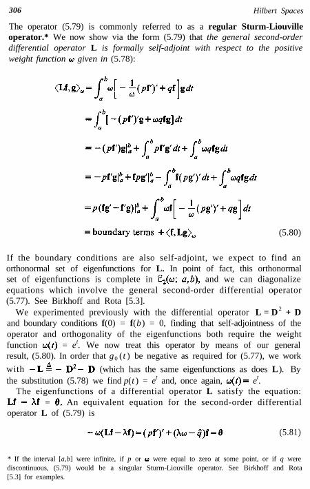
306 Hilbert Spaces

The operator (5.79) is commonly referred to as a regular Sturm-Liouvilleoperator.* We now show via the form (5.79) that the general second-orderdifferential operator L is formally self-adjoint with respect to the positiveweight function c3 given in (5.78):

(5.80)

If the boundary conditions are also self-adjoint, we expect to find anorthonormal set of eigenfunctions for L. In point of fact, this orthonormalset of eigenfunctions is complete in h(o; a,b), and we can diagonalizeequations which involve the general second-order differential operator(5.77). See Birkhoff and Rota [5.3].

*

We experimented previously with the differential operator L = D2 + Dand boundary conditions f(0) = f(b) = 0, finding that self-adjointness of theoperator and orthogonality of the eigenfunctions both require the weightfunction w(t) = et. We now treat this operator by means of our generalresult, (5.80). In order that g0 (t ) be negative as required for (5.77), we work

with -LA - D2- D (which has the same eigenfunctions as does L). Bythe substitution (5.78) we find p(t ) = et and, once again, o(t)= et.

The eigenfunctions of a differential operator L satisfy the equation:Lf - Xf = 8. An equivalent equation for the second-order differentialoperator L of (5.79) is

- o(Lf - hf) = (pf’)’ + (X0 - i)f = 8 (5.81)

* If the interval [a,b] were infinite, if p or w were equal to zero at some point, or if q werediscontinuous, (5.79) would be a singular Sturm-Liouville operator. See Birkhoff and Rota[5.3] for examples.


where 4 A oq. Equation (5.81) is known as a regular Sturm-Liouvilleequation. For certain boundary conditions on f, L will have eigendata. Ifthe boundary conditions are self-adjoint with weight w, the eigenfunctionscan be chosen so they are orthonormal with weight w. We can obtain theeigendata from (5.81) and the boundary conditions. We call (5.81) togetherwith self-adjoint boundary conditions a regular Sturm-Liouville system.

Decoupling of Equations By Means of Eigenvector Expansion

We wish to analyze the linear equation Tx = y, wherein x and y aremembers of a separable infinite-dimensional Hilbert space X. We havefound that we can have orthonormal eigenvectors of T only if T isself-adjoint. It can be shown that complete continuity of T is sufficient(but not necessary) to guarantee that the eigenvalues and eigenvectors of Tare countable. Furthermore, complete continuity together with self-adjointness guarantees that eigendata exist and, that the eigenvectors arecomplete in X .* We assume T is self-adjoint and completely continuous;then the spectral theorem (5.74) applies, and T is diagonalizable by meansof an orthonormal eigenvector basis {xk }. The vectors x and y can beexpanded using (5.72):

y= 5 ckxk and x= 5 dkxkk=l

(5.82)

where ck = (y, xk), and can be computed using the known vector y; dk isthe kth Fourier coefficient of the unknown solution vector x. We substitutethe expansions (5.82) into the equation Tx = y to find

e=y--TX= 5 C&--Tk-l

k=l k=l

= c @k-hkdk)xk

where we have relied on the continuity of T and (5.56) to take T inside theinfinite sum. Then using the orthonormality of the basis {x k }, we find

O= lb-Txl12= 11 @k -hkdk)xkii2=

* See Bachman and Narici [5.2, Chapter 24] and Stakgold [5.22, Chapter 3].

308 Hilbert Spaces

Since each term in the sum is non-negative,T is invertible (i.e., has no zero eigenvalues),

O” bxk)X= c

k=l

Ck=Akdk,k= 1,2,…. Then, if

(5.83)

Equation (5.83) is an explicit expression of the solution x to the equationTx = y in terms of the eigendata for T. The fact that T is assumed to act ona Hilbert space is not really a restriction. Were X an incomplete innerproduct space, it could be completed and the definition of T extended tothe complete space. Furthermore, we are not significantly hampered by theboundedness (or complete continuity) used in the derivation of (5.83).Suppose, for example, that T represents a self-adjoint differential operatorwith its boundary conditions (an unbounded operator). If the boundaryconditions are appropriate, T is invertible and T-l is typically bounded(and perhaps completely continuous). We simply replace Tx = y by T- 1y= x, and repeat the above argument to find again that dk = ck/hk and(5.83) is valid.

Example 4. Analysis of a Differential System by Eigenfunction Expansion. Theshaft position +(t) of a dc motor (with prescribed initial and final shaft positions) isrelated to the armature voltage u of the motor by the following differentialequation and boundary conditions:

L&j++“, +(O)=+(b)=0

The Green’s function (3.42) for this system is bounded. Therefore, the inverseoperator is Hilbert-Schmidt and, consequently, completely continuous. Further-more, the differential system is self-adjoint relative to the weight function w(t) = et,as noted in Exercise 4. The eigenvalues and eigenfunctions for this differentialsystem are given by (4.37) and (4.38):

&=-f-($r, f~(t)=~e-‘/2Qin(~), k-1,2,...

We determined in Example 3 of Section 5.3 that these eigenfunctions areorthogonal relative to the weight function which makes the differential systemself-adjoint. (We have added the multiplier m in order to make the functionsorthonormal.) We also showed in that example that these eigenfunctions form abasis for (? (e’; 0, b). [Of course, it is also a basis for the completion of that space,!Z,(e *; 0, b).j We now use (5.83) to express the solution to the differential system asan expansion in the eigenfunctions of the system; + takes the role of x , y becomes


u, and xk becomes fk :

(5.84)

The solution to this differential system was obtained by inversion in Section 3.3.Following (3.42) we used the inverse to determine the solution for the inputu(t ) = 1:

+(t)= t- -j$ (1 -e-‘)

For this same input, u(t)= 1, (5.84) becomes

In Figure 5.10, we compare the exact solution with the first two terms of theeigenfunction expansion for b = VT.. It is apparent from the figure that for allpractical purposes the first few terms of the series determine the solution.

Example 5. Using the eigenfunctions of Example 4, compute the first twoterms of the eigenfunction expansion of the input u ( t ) = 1 with b = ?T.(Hint: multiply each curve of Figure 5.10 by the appropriate eigenvalue.)Note that the convergence of this series is considerably slower than theconvergence of the output function c/(t). Furthermore, the series does notconverge at the endpoints; convergence in the e2 norm does not implyconvergence everywhere.

0.25

0

-0.25

-0.5

-0.75

-1.0

-1.25

Figure 5.10. Convergence of (5.84) for u(t) = 1 and b = T.

310 Hilbert Spaces

Suppose that T is self-adjoint and completely continuous, but is notinvertible. Then the equation Tx = y has no solution unless y is in range( T ) .Furthermore, if the equation has a solution, we can add to it any vector innullspace to obtain another solution. Formal application of (5.83)would require division by a zero eigenvalue. To resolve this difficulty, wedecompose the equation. By the orthogonal decomposition theorem (5.67)and the self-adjointness of T, V = nullspace(T ) range(T ). Those eigen-vectors in the orthonormal basis which are associated with the zeroeigenvalue form an orthonormal basis for nullspace(T). The remainingeigenvectors form an orthonormal basis for range(T ). Moreover, the actionof T on range(T) is one-to-one (the zero eigenvalues have been removed).We use (5.83) to obtain a particular solution to the equation Tx = y bysumming over only the nonzero eigenvalues; the resulting solution lies inrange(T). Assuming y is in range(T), the general solution to the equationTx = y, for a self-adjoint completely continuous transformation T, is ex-pressed in terms of the eigendata for T by

X= c(Yyxk)x +x

Ak k o(5.85)

nonzeroAk

where x0 is an arbitrary vector in nullspace(T ). As with (5.83), (5.85) maybe valid even though T is not completely continuous. This fact is il-lustrated by the unbounded differential operator of Example 5. Ratherthan dwell further on conditions wherein (5.85) is valid, we adopt the(possibly risky) course of assuming its validity whenever the equation isuseful.

In principle, in order to determine whether or not Tx = y has solutions,we must solve explicitly for range(T) and see whether or not y is inrange(T ). Finding range(T) directly can be difficult for, say, a differentialoperator. It is simpler to apply the orthogonal decomposition which wasintroduced in the previous paragraph. If T is self-adjoint and range(T ) isclosed,

Ir = nullspace(T ) & range( T )

We solve Tx = 8 for the vectors in nullspace(T). Then, rather than expli-citly determine the vectors in range(T), we simply check to see whether ornot y is orthogonal to all vectors in nullspace(T); y will be orthogonal tonullspace( T ) if and only if it lies in range(T). Although the range of adifferential operator is not closed, this orthogonality test for existence of asolution is used most often for differential equations. See Friedman [5.8,Chapter 3].


Example 5. Analysis by Eigenfunction Expansion—a Noninvertible Case. Let T

represent the differential operator L b D2 with the homogeneous boundary condi-tions f( 1) - f(O)=f’( 1) -f’(O) = 0. The operator T is self-adjoint with respect to thestandard function space inner product. However, T is degenerate; the differentialsystem

f” = u, f(l) =m, f’(l)=f’(O)

has solutions only for a restricted set of functions u. Nullspace consists in thesolutions to the completely homogeneous system,

f”(t)=O, f(l) =m rl(l)=tl(O)

Thus nullspace consists in the “constant functions,” f0 (t ) = c. By the discussionabove, u can be in range(T) only if u is orthogonal (with respect to the standardinner product) to nullspace(T). Therefore, in order that the differential system havea solution, u must satisfy

(u,fJ= jo’u(s)ch=O

for all constants c; that is, $tu(s)ds = 0. The constant functions are eigenfunctionsof T for the eigenvalue A, = 0. The nonzero eigenvalues and the correspondingeigenfunctions can be determined by the techniques of Section 4.3; they are

Ak = - (2rk)*, f,(t) = fi cos2vrkt, gk( t) = fi sin 2rkt

for k = 1,2,.... Note that there are two eigenfunctions, fk and gk, for eacheigenvalue. The orthogonality of the eigenfunctions for different eigenvalues fol-lows from the self-adjointness of T. Each pair of eigenfunctions has been selectedsuch that it forms an orthogonal pair. The whole set of eigenfunctions is essentially(5.30), the basis for the classical Fourier series; the constant function is missingsince it is not in range(T). If 1, u(s)ds = 0, the solution to the differential systemcan be expressed by the eigenfunction expansion (5.85):

312 Hilbert Spaces

The arbitrary constant c expresses the freedom (or nonuniqueness) in the solution.As in Example 4. comparison of the exact solution with the sum of the first fewterms of the series for a specific u demonstrates that convergence of the series israpid.

We found earlier that the general second-order differential operator(5.77) is formally self-adjoint with respect to the weight function o of(5.78). If the boundary conditions are also self-adjoint, the second-orderdifferential operator (or regular Sturm-Liouville operator) has eigendata;these eigendata are determined by (5.81) together with the boundaryconditions. It can be shown that the solutions (eigenfunctions) of anyregular Sturm-Liouville system are complete; they form a countable basis,orthonormal with respect to weight o, for the space E,(a,b).* As exempli-fied by Example 4, it can also be shown that any regular Sturm-Liouvillesystem has an infinite sequence of real eigenvalues h, < h, < X, < * * . . (Ifthe differential operator is invertible, its inverse is a Hilbert-Schmidtoperator; that is, the inverse is completely continuous.) Furthermore, theeigenfunctions for a regular Sturm-Liouville system are similar to thesinusoidal functions in that the eigenfunctions for the n th eigenvalue haven zero crossings in the interval [a,b]. Sturm-Liouville problems are typi-cally steady state (or standing-wave) problems. Examples of physicalsystems modeled by regular Sturm-Liouville operators and self-adjointboundary conditions are vibrating strings, beams, and membranes. Steady-state heat flow in one dimension is another example. Less typical is themotor control problem introduced in (3.40) and solved by eigenfunctionexpansion in Example 4. In this problem, the standing-wave nature arisesbecause conditions are placed on the future position of the motor shaft.

It follows from Parseval’s identity (5.48) that the Fourier coefficients ofa vector x relative to a countably infinite orthonormal basis {x k } mustapproach zero: (x,x,)+0 as k-co. It is evident from Examples 4 and 5that the convergence of eigenvector expansions of solutions is accountedfor only in part by this property of the Fourier coefficients. In general,Fourier coefficients converge at least as fast as l/k. However, in thesesecond-order examples a stronger influence on the convergence of thesolutions is exerted by the eigenvalues, with l/X, converging approxi-mately at 1/k2. The “output expansion” (or solution) consists in a modifi-cation of the eigenfunction expansion of the input, wherein high-ordereigenfunction components (or normal modes) of the input are attenuatedmore than are the low-order components. In analogy to a dynamic systemwith initial conditions, we can think of the systems of Examples 4 and 5 as“low-pass” systems; the systems emphasize (or pass) the low-order eigen-functions.

*See Birkhoff and Rota [5.3].


Example 6. Solution of a Partial Differential Equation by Eigenfunction Expansion.The following partial differential equation is a model for problems in electrostaticsor heat flow:

Vf=u

Let the two-dimensional region Q of the (s,t) plane on which f and u are defined bethe rectangle 0 < s Q a, 0 Q t Q b. Let f(s,t) = 0 on the boundary I of this rectangle.In Example 11 of Section 5.4, we determined that V* is formally self-adjoint withrespect to the standard inner product (5.64). Furthermore the boundary conditionis also self-adjoint. Thus we expect to find a basis for &,(SQ consisting inorthonormal eigenfunctions of the differential system. The eigendata for the systemare given in (4.62) and (4.63); we express the eigenfunctions in normalized form:

Ln= -( 7)2-( 7)2= - -$n*a’+m*b*)

fmn(s, 0 = --&sin(~)sin(~)

It can be shown that these eigenfunctions are complete in fZ2(Q) [5.22, p. 1931. By(5.83), the solution to the differential system, expressed as an eigenfunctionexpansion, is

fh 0

We have no closed form solution with which to compare this result. Rather,techniques for finding Green’s functions for partial differential operators areusually based upon eigenfunction expansions similar to the one used here. See(5.86).

Further Spectral Concepts

We have developed two different approaches to the solution of an invert-ible differential system, the inverse (3.35) and the eigenfunction expansion(5.83). We would be surprised if the two techniques were not closelyrelated. Let the differential operator L act on a space of functions definedon [a,b ]. Suppose L together with homogeneous boundary conditions haseigendata {hk,fk}. Further assume that the eigenfunctions form a basis forthe function space which is orthonormal with respect to the standard innerproduct. We wish to explore the equation Lf = u together with theboundary conditions. The solution f can be expressed in terms of theGreen’s function k(t,s) as f(t)=I,bk(t,s)u(s)&. As discussed in Chapter 3,

314 Hilbert Spaces

the Green’s function is the solution corresponding to the input u ( t ) =Using (5.83) we express this solution in terms of the eigendata:

(5.86)

Equation (5.86) is known as the bilinear expansion of the Green’s functionfor L in terms of the eigenfunctions of L. The Green’s function for theLaplacian operator is in fact derivable from Example 6 using an extensionof (5.86) to a space of two-dimensional functions.

Exercise 6. Find the bilinear expansion of the Green’s function forExample 4 and compare the first term to the exact Green’s function asexpressed in (3.42).

The spectral theorem (5.74) can be used to define functions of linearoperators analogous to the functions of matrix operators discussed inSection 4.6. Assume the linear operator T in the Hilbert space Y isself-adjoint and completely continuous. Then, applying T to the expansion(5.72) of a general vector x in terms of an orthonormal set { xk } ofeigenvectors for T, we find

‘I-X= g &(x,xk)xkk-1

(5.87)

where we have used the continuity of T in order to take T inside theinfinite sum. By combining all terms of (5.87) which are associated withidentical eigenvalues, we reexpress (5.87) as

T= E XjPjj = 1

(5.88)

where P j is the orthogonal projector onto nullspace Thus theeffect of Pj on a general vector x in V can be expressed in terms of theorthonormal eigenvectors of T:

q x = x (x,x,)x, (5.89)k


where the summation is over all values of k which correspond to theeigenvalue xi. Equation (5.88) is the spectral decomposition of T; it can beinterpreted as a diagonalization of T. If f is a real continuous functionwhich is defined at the eigenvalues of T, it can be shown that a suitabledefinition of a function of a transformation is provided by the fundamentalformula for f (T):

f(T)= 5 f(‘j)” (5.90)j-1

Although we have defined (5.90) only for a self-adjoint, completely con-tinuous T, the definition can be extended to any bounded normal lineartransformation.* Furthermore, as we know from our examples, it canapply to unbounded differential operators. Equation (5.83), for instance, is

essentially an expression of x = f (T)y for the function f(t) 9 t -l. Weapplied (5.83) to an unbounded differential operator in Example 4.

Throughout our examination of infinite-dimensional operator equations,we have restricted ourselves to operators for which there is a countableorthonormal set of eigenvectors which form a basis for the space. Self-adjoint, completely continuous transformations are of this type. We haverestricted ourselves to these transformations in order to work with only thesimplest infinite-dimensional extensions of matrix equations. More general-ity comes only with considerably increased abstraction. Let T be a linearoperator on an inner product space Y. The eigenvalues and eigenvectorsof T are determined by the equation Tx =Xx, or alternatively, by theresolvant operator, (I’ - AI)- ’ ; the eigenvalues of T are those values of A forwhich the latter inverse does not exist. However the nonexistence of theinverse is only one of the ways in which the resolvant operator can be“irregular.” Detailed discussions of the resolvant operator and generalspectral concepts can be found in Bachman and Narici [5.2], Stakgold[5.22], Friedman [5.8], and Naylor and Sell [5.17].

Matched Filter Design–An Application of Spectral Decomposition

We wish to recognize the presence or absence of a signal u ( t ) of knownshape (e.g., a radar return). Our measurement of the signal is corrupted by

stationary noise n(t) whose autocorrelation function, R(t,s) b E[n(t) n(s)]= R( t - s ), is known. Because n(t ) is stationary, R is symmetric in t and s,and depends only on the time difference t - s ; R is also finite and positive.We filter the noisy measurement in order to improve our estimate of thepresence or absence of the signal (see Figure 5.11). We select the impulse

* Bachman and Narici [5.2].

316 Hilbert Spaces

Figure 5.11. A linear filter.

response h(t) of the linear filter in such a way that the signal-to-noise ratioof the output, ug(b)/E[&b)], is maximized at some time t = b units aftermeasurement begins. [A circuit can then be synthesized which has theimpulse response h(t).] The output signal and noise at time t = b are,respectively,*

y,(b)= kbh(s)u(b-s)dr

q,(b)=i’h(s)n(b-s)ds

Then

E[d(b)] =Elbh(s)n(b-s)dr/bh(t)n(b- t)dt0 0

=Jl

’ ‘h(s)h(t)R (s- t)dtds0 0

We use the concepts of P&C 5.30 and Exercise 3, Section 5.1 to interpret

E[&$b)] as the square of a norm. Define T by (l%)(s) A l,bh(t)R (s- t)dt.Then, since R is positive and symmetric in its variables, T is self-adjoint,completely continuous (Hilbert-Schmidt), and positive definite; T is di-agonalizable by means of an orthonormal basis of eigenfunctions {f k }, andthe eigenvalues {&} of T are positive (P&C 5.28). Therefore, the square

roots { fi } exist, and a unique self-adjoint positive-definite operatorfl is defined by (5.90). Thus

E[ G(b)] = ~bh(ww) ds

= (h, n)

* See Appendix 2 for a discussion of convolution and impulse response.


Let ur denote the “reverse” of the signal shape u; that is, ur (s) i u( b - s).Then u0 (b) = (h,u,). Since the eigenvalues { 6 } of fl are all positive,fi is invertible and range( ) is the whole function space, C2(0, b).Therefore, we can assume ur is in range (fi ); that is, ur = fl g for somefunction g. Then

u;(b)= I(h,U,))2= I+, fl g>12= I<fl h,g>12

As a consequence, the signal-to-noise ratio satisfies

4(b) = I(fl h)12E[ 4(b)] II fi hII2

( llgl12

The latter relationship is the Cauchy-Schwartz inequality (P&C 5.4);equality holds if fl h = cg for any constant c, or Th = cm g = cur. Wemust solve this integral equation for h. It is apparent that h depends onlyon the shape of the signal u, but not its magnitude. We can express thesolution to the equation in terms of eigendata for T by means of (5.83):

h=cx 7 kO” +,,fk> f

k-l k

Suppose the noise is “white”; that is, the autocorrelation function is thelimiting case R(s - t) = N6 (s - t), where N is the noise power and 6 (s - t)is the Dirac delta function. The integral equation becomes

(Th)(s)=N~bh(t)~(s-t)dt=Nh(s)=cur(s)0

or h(s) is any multiple of ur (s ) = u(b - s). The optimum impulse responsefor this case has the form of the signal running backward in time from thefixed time t = b. A filter with this characteristic is called a matched filter.We can also use the eigenfunction expansion to determine this solution:The eigendata are determined by

(l-b)(s) = Nh(s) =Ah(s)

The only eigenvalue is h= N. Every function is an eigenfunction. Letting{fk } be any orthonormal basis for the space, the eigenfunction expansionbecomes

318 Hilbert Spaces

The eigenfunction expansion is just a Fourier series expansion of ur .Although we easily solved for this matched filter, solution of an integralequation and determination of the eigendata of an integral operator areusually difficult problems.

5.6 Problems and Comments

5.1 Let A be a real symmetric 2x2 matrix with positive eigenvalues.(a) Show that the curve described by the quadratic equation

(x, Ax) = xTAx = 1 is an ellipse in the x plane. Determine therelationship between the ellipse and the eigendata for A.(Hint: a symmetric matrix has orthogonal eigenvectors.Therefore it can be diagonalized by means of the transforma-tion A = STAS.)

(b) Find the eigendata and sketch the ellipse for

5.2 Show that the following definition satisfies the rules for an innerproduct on 9%‘:

5.3 Let Y and W be inner product spaces over the same scalar fieldwith inner products denoted by ( , )y and ( , >%, respec-tively. Let u and v be in V; let w and z be in ‘?K.(a) Show that the following is an inner product on the Cartesian

product space ‘v X % : ((u, w), (v, z)) 2 (u, v), + (w, z),(b) Let x and y denote vectors in C2(0, 1) X &?‘(O, 1). Express the

elements of x and y as 2 x 1 matrices rather than as 2-tuples.(Then for each t in [0,1], x(t) and y(t) are in the state space,

9R2” ‘.) Show that the inner product (x, y) A Jo’ y’(t)x( t) dt i sessentially a special case of the inner product defined in (a).

*5.4 The following useful equalities and inequalities apply to the vectorsin any inner product space Ir:(a) Pythagorean theorem: if (x, y) = 0, then

llx+Yl12= llxl12+ llYl12

(b) Bessel’s inequality: if {xi} is an orthonormal set in ‘v, then

llxl12 ’ C ICx9 xi>l2i

Sec. 5.6 Problems and Comments 319

(c) Parseval’s identity: equality occurs in (b) if and only if {x i } isa basis for Ir;

(d) Cauchy-Schwartz inequality: I(x,y>I Q llxllI]yll, with equality ifand only if x and y are collinear;

(e) Triangle inequality: Ilx+ yII Q llxll+ Ilyll.5.5 Equip the vector space CR2 with the inner product

where 5i and 77i are the components of x and y, respectively.(a) Find the matrix QG of the inner product relative to the

standard basis for C!R2;(b) Find the matrix QX of the inner product relative to the basis

‘?C A {(l,O),(l,l)}. Explain the simple form of Q%.Let ( , ) be an inner product defined on an n-dimensional space?f. Let QX and Q3 be the matrices of this inner product relativeto the bases ?C and 94 , respectively. Let S be the coordinatetransformation matrix defined by [xl% = S[x]% .(c) Determine the relationship between Q%, Q%, and S;(d) What special property does S possess if ‘% and 3 are both

orthonormal?

5.6 The set ‘?X A {(1,1),(0,-1)} is a basis for %2. Find an innerproduct which makes the basis ‘2X orthonormal. Determine thematrix QG of this inner product relative to the standard basis for5L2 .

5.7 Let

The set 9C = {x1 ,x2 ,x3} is a basis for %3x1.(a) Determine an inner product for %3x ’ with respect to which

the basis is orthonormal.(4 Find QG, the matrix of the inner product relative to the

standard basis for %3x ‘.5.8 Let %, be the subspace of q3 which is spanned by the pair of

vectors (1,0,1) and (0,1,-1). Let (?K2 be the subspace of a3 whichis spanned by the vector (1,1,1). Pick an inner product for a3which makes every vector in q$, orthogonal to every vector in w2.

*5.9 Positive-definite matrices: a symmetric n x n matrix A is calledpositive definite if xTAx > 0 for all real n X 1 vectors x and if

320 Hilbert Spaces

equality occurs only for x = 8. Suppose we pick the kth componentof x equal to zero; it follows that the submatrix of A obtained bydeleting the kth row and kth column of A must also be positivedefinite. In fact, any principal submatrix of A (obtained by deletinga set of rows and the corresponding columns of A) must be positivedefinite. The determinant of a matrix equals the product of itseigenvalues (P&C 4.6). Furthermore, the eigenvalues of a positivedefinite matrix are all positive (P&C 5.28). Consequently, if A ispositive definite, the determinant of A and of each principle sub-matrix of A must be positive.

Let Ar be obtained from A by deleting all but the first r rows andcolumns of A; det(Ar) is called the rth leading principle minor of A.A symmetric n X n matrix A is positive definite if and only if the nleading principle minors of A are positive (see [5.14] and [5.25]).Checking the sign of the leading principle minors is a convenienttest for positive definiteness of A.

5.10 Show that the statement (A, B) = trace(BTA) defines a valid innerproduct on the real vector space aRx” ; (the trace of a squarematrix is defined to be the sum of the elements on its maindiagonal).

5.11 Let % B {x1, . . . ,xn } be an orthonormal basis for a vector space ‘V.Let T be a linear operator on V. Then the element in row i,column j of [T],, is (Txj,xi) for i , j = 1,. . . , n.

5.12 Let ‘?X = {x1 ,x2,... } be an orthogonal basis for a real inner productspace V. Approximate a vector x of V by a linear combination,xa =Xg=ickxk, of the first n vectors of !X in such a way thatI]x-x~]]~ is minimized. Show that the coefficients {c k} are theFourier coefficients. How are the coefficients affected if we im-prove the approximation by adding more terms to xa (increasingn)?

5.13 Let A be a 3 X 3 matrix with eigenvalues andcorresponding linearly independent eigenvectors x1, x2, and x3. Let(. , a) denote an inner product for which the above eigenvectors areorthonormal. We wish to solve the equation Ax = y.(a) Assuming solutions exist, express the general solution x in

terms of the eigendata and the inner product.(b) Determine the conditions that y must satisfy in order that

solutions exist. Express these conditions in terms of the ei-gendata and the inner product.

5 .14 Equip %3x1 with the standard inner product, x,y k yTx . Let


x,=&2=($ x3=Q-2 Obtain an orthonormal basis for span

{x 1, x2, x3} by applying the Gram-Schmidt procedure to {x 1 , x2 , x 3}.

5.15 Assign to %3x ’ the inner product (x, y) 4 yTQx, where

Let x1 = (1 0 1)T. Find an orthogonal basis for {x1 } *, the ortho-gonal complement of x1 .

*5.16 Recurrence formulas for orthogonal polynomials: let {p 0 , p1 , p2, . . . } bea set of polynomials orthogonal with respect to some inner product.Then pn can be expressed in terms of pn -1 and pn -2 in thefollowing fashion:

p,(t) = (q + 4JPn- l(t) - %IPn-2w

Once the appropriate coefficients {a n, bn, cn} are known, the three-term recurrence formula allows successive determination of theorthogonal polynomials in a manner which is far less cumbersomethan the Gram-Schmidt procedure [5.7]. Three-term recurrenceformulas exist for other orthogonal sets as well: sine-cosine func-tions, Bessel functions, and various sets of functions defined ondiscrete domains. (See [5.24], p. 269 and [5.12]).

Verify for n = 2 that the Legendre polynomials of Example 2,Section 5.2 obey the recurrence relation

PW (= 2n-1

n -) tp,&) - (V)Ptz-2wn

Use this recurrence relation to compute p3 and verify that it is thenext polynomial in the Legendre polynomial set; that is, show thatp 3 has the correct norm and is orthogonal to the lower-orderpolynomials in the set.

5.17 Let 03( - 1,l) be the ‘space of real polynomial functions of degreeless than three with the inner product

322 Hilbert Spaces

Let (?!I! be the subspace of T3( - 1,l) spanned by f0, where

f0 (t) 2 1. Find a basis for qt’-, the orthogonal complement of ‘%‘.

5.18 Let Ir be the space of complex-valued functions on [0,l] which arebounded, piecewise continuous, and have no more than a finitenumber of maxima, minima, or discontinuities (these are called theDirichlet conditions). A typical function in V is

Equip Ir with the inner product

(f,g) A j-‘f(t) g(t) dt0

Then the set of functions

g,(t) 2 ei- n=o, k 1, ?2,...

where i=d?, is an orthonormal basis for the space.(a) Determine the coordinates of the function h relative to this

orthonormal basis; that is, expand h in its exponential Fourierseries.

(6) To what value does the series converge at the discontinuities(t = 0, i, l)? (Hint: combine the positive and negative n t horder terms of the series.)

*5.19 Let T be the linear operator on %zxl defined by

TX 9 Ax

where A is an n x n matrix. Let the inner product on %:x ’ bedefined by

(x, Y> = Y=Qx,

where Q is a hermitian-symmetric, positive-definite matrix.Determine the form of T*.

5.20 Let T be the linear operator on the standard inner product spaceI;,(O, 1) defined by

(Tf)(t) A jlb(s)f(s)ds0

Determine the form of T*. Hint: watch the limits of integration.


5.21

5.22

5.23

5.24

5.25

5.26

Let T: I;,(O, 1) X E2(0, I)+ %2x1 be defined by

Tu AJ 'Q(s)u(s)d~

0

where Q(s) is a 2 x 2 matrix and u(s) is a 2 X 1 matrix. Find theadjoint T* for the inner products

(x,y)~2”1 A y’x

k s1

(u,v)e* x e2 v’( s)u( s) ds0

Let (x,z>, L zTQx and (y,w), A wTRy specify the inner productson the real spaces Wx ’ and ?IRmx ‘, respectively, where Q and Rare symmetric, positive-definite matrices. Define T: EXn x ‘-+ Xrn x ’

by TX A Ax.(a) Find T*.(6) Determine the properties which must be satisfied by A, Q,

and R in order that T be self-adjoint.

Define T on ‘?JE2”’ by Tx A Ax, where A = Define the

inner product by (x, y) = yTQx. Pick Q such that T is self-adjoint.

Let L i D2 +D act on those functions f in CZ2(a,6) which satisfy theboundary conditions f (a) = f’(6) = 0. Assuming the standard innerproduct for Ci?‘(a,b), find the formal adjoint L* and the adjointboundary conditions.

Define the differential operator L on e2(a,6) by Lf A f” - f’. As-sociate with L the boundary conditions f(a) + f’(a) = f(6) + f’(6) = 0.Find the formal adjoint L* and the adjoint boundary conditionsrelative to the standard inner product.

The wave equation is

where s and o are space variables and t represents time. Thisequation can be represented in operator notation as

(V” - D2)f = 8

where the Laplacian operator V2 acts only with respect to the spacevariables and the ordinary differential operator D2 acts only withrespect to the time variable. Assume V*-D* acts on the space

324 Hilbert Spaces

e,(a) X C2(0, 6) with the inner product

(fd= /“/f(p,f)g(p,t)dpdt0 clwhere p = (s, a), Q is the spatial domain (with boundary I), and t isin [0,b]. Show that the “wave operator” V2- D2 is formally self-adjoint. Hint: use Examples 10 and 11 of Section 5.4.

*5.27 Let ‘v be an inner product space (perhaps infinite dimensional)with a basis %. Let T be a linear operator on ?r. Show that if %is orthonormal, [T*lXX =[TlT3CX. Hint: express the inner productin terms of coordinates relative to the orthonormal basis.

*5.28 Let T be a linear operator on a complex inner product space v.(a) (1) If T*T = we call T a normal operator.

(2) If T*T = TT* = I (i.e., T* = T -1), we call T a unitaryoperator.

(3) We call T non-negative if (TX, x) > 0 for all complex x inV. If, in addition, (Tx,x) = 0 only for x = 8, we say T ispositive definite.

(6) If T is (1) self-adjoint, (2) non-negative, (3) positive definite,(4) unitary, or (5) a projector, then the eigenvalues of T are,respectively, (1') real, (2') non-negative, (3') positive, (4') ofabsolute value 1, or (5') equal to 1 or 0. If T is normal and vis finite dimensional, then (1')-(5') also imply (1)-(5). Theinclusions among these classes of linear operators are il-lustrated by the following diagram.


*5.29 Norms of linear transformations: define T: ‘%z x ’ + ‘%T x ’ by

TX&%X, where A is an mxn matrix. Assume the standard innerproducts. Then

where h, is the eigenvalue of ATA which is of largest magnitude.(a) Find l]Al] for the following matrix by carrying out the max-

imization indicated above:

(6) Find ]]A[] for the matrix A of (a) by determining the eigen-value h,.

(c) A coarse, but easily computed, upper bound on ]]A/ is theEuclidean norm of A defined by

llAll$ A c IaJ’= trace( ATA) = trace(AAT) = 2 IAilid i

(The numbers {xi} are the eigenvalues of A.) Find l]AllE for

(djthe matrix A of (a). (The last of the equalities applies only for square A. )If T is a bounded normal operator on a complex Hilbert spaceIr, then

IITII = ,;FI I(TJ->I = “” l&l

where the numbers {xi} are the eigenvalues of T [5.2, p. 382].Use this relationship to find l]T- ‘I] for T equal to the differen-tial system of Example 2, Section 4.3. Note that this re-lationship between l]Tl] and the largest eigenvalue of T can beused to determine [IAll for any symmetric matrix A; it cannotbe used for the matrix A of (a).

*5.30 Let T be a bounded linear operator on a Hilbert space V.

(a) Show that (x, y), A (x,Ty) is an inner product on ‘V if andonly if T is self-adjoint and positive definite.

(6) The operator T is self-adjoint and positive definite if and onlyif T can be decomposed as T = U2 where U is a self-adjointpositive-definite linear operator on Ir.

(c) L e t V=CX2x1 with the standard inner product. Let Tx A Qx

326 Hilbert Spaces

where

Find a self-adjoint, positive-definite operator U on %2x rsuch that T = U2 .

*5.31 Reciprocal bases: let { x1 , ... , xn } be a basis for snxl which iscomposed of eigenvectors for the invertible n x n matrix A . Assumethe standard inner product for 91Lnx ‘. The reciprocal basis{y l , …, yn } (reciprocal to {xi}) is defined by (xi, yj) = y;x,. = aO.(a) The vectors in the reciprocal basis are eigenvectors of AT

(left-hand eigenvectors of A) .(b) Every vector x in W x ’ can be expressed as a biorthogonal

expansion, x = IX:- ,(x, yi)xi. Use this fact to show that thesolution to Ax = y can be expanded as

Hint: follow the derivation of (5.24).(c) The outer product of two vectors in W x ’ is defined by

x><yA xyT. Such a “backwards inner product” is sometimesreferred to as a dyad. Use the dyad notation to convert theexpansion in (b) to an explicit matrix multiplication of y .Compare the resulting matrix to the fundamental formula forA - 1,

A - 1 =

where p is the number of distinct eigenvalues of A . How arethe constituent matrices {ETO} related to the pair of biortho-gonal bases {xi} and {y i}?

(d) Let A = Find a basis for 9R,2x1 consisting in

eigenvectors for A; find the reciprocal basis; use the pair ofbiorthogonal bases to find the constituents of A; use theconstituents to compute A- 1.

5.32 Let A be an n x n matrix. Then TX *on Xnxl.

= Ax defines a linear operator TLet Q be an n x n symmetric positive-definite matrix.

(a) Show that if T is self-adjoint with respect to the inner product


(x,Y)~ k yTQx, then the operator U defined by Ux g QAx isself-adjoint with respect to the standard inner product. Thematrix equation Ax = y can be replaced by an equivalentequation, QAx = Qy; the latter equation can be analyzed interms of a set of eigenvectors (of QA) which is orthonormalwith respect to the standard inner product.

Let A = Find a matrix Q such that T is self-adjoint

with respect to the inner product (x, Y)~ = yTQx.for positive definiteness is given in P&C 5.9.

Hint: a test

5.33 By Example 2, Section 5.5, the differential operator L A -D2 andthe boundary conditions f(0) = f (b) = 0 are self-adjoint with respectto the standard inner product on the interval [0,b ].(a) The eigendata for L with the given boundary conditions are

k = 1,2,3,...

Show that the eigenfunctions form an orthogonal set.(b) Express the solution to the differential system -f" = u, f(0)

= f(b ) = 0 as an eigenfunction expansion.(c) Compare the first term of the eigenfunction expansion in (b)

to the exact solution for the specific input function u(t ) = 1and b = 1.

5.34 The (nonharmonic) eigendata for the differential operator -D2

with the boundary conditions f(0) = f(b) + f'(b) = 0 are derived inExample 1, Section 4.3.(a) Show that the eigenfunctions are orthogonal with respect to

the standard inner product on the interval [0,b ] (and, con-sequently, that L and the boundary conditions are self-adjoint).

(b) Express the solution to the differential system -f" = u, f(0)= f (b) + f'(b) = 0 as an eigenfunction expansion.

(c) Compare the first term of the eigenfunction expansion in (b)to the exact solution for the specific input u( t ) = 1 and b = 1.Hint: tan(2.0288) -2.0288. (The exact solution for thedifferential system is given in P&C 3.13. Note that the sym-metry of the Green’s function again implies the self-adjointness of the system with respect to the standard innerproduct .)

5.35 A (nonsinusoidal) periodic voltage e of frequency w (period 277/o)

328 Hilbert Spaces

is applied to the terminals of the R-L circuit of Figure 5.4. Thesteady-state current i1 satisfies the differential equation Li; + Ri,= e with the periodic boundary condition il(2T/o) = i,(O).(a) Find the eigendata for the differential operator LD + RI with

periodic boundary conditions.(6) Show that the eigenfunctions are orthogonal with respect to

the standard complex inner product on the interval [0,2~/0].(c) Determine the eigenfunction expansion of the steady-state

current for an arbitrary periodic voltage. Verify the result byapplying the voltage e(t) = sin wt.

5.36 Define V2f(s, t) k (a2f/as2)+(a2f/at2) on the rectangle 0 < s < a ,0 d t Q b. Let f satisfy the boundary conditions

=$O,t)= z(a,t)= g(s,O)= $(s,b)=O

(a) The eigendata for V2 with the given boundary conditions aredisplayed in P&C 4.15. Show that the eigenfunctions areorthogonal with respect to the inner product

(f,g) A ~blaf(s,t)g(s,+hdf0 0

(6) Note that one of the eigenvalues is zero. The range of theoperator was derived in Example 12, Section 5.4. Express asan eigenfunction expansion the general solution to the partialdifferential system V*f = u with the given boundary conditions.

*5.37 A Hilbert space of random variables: let ?r be a vector space ofreal-valued random variables defined on a particular experiment(Example 11, Section 2.1). An inner product can be defined on Irin terms of the expected value operation (P&C 2.23):

(x, y> A E(xy) = x(σ)y(σ) ω(σ) dσ

(a) Show that E(xy) is a valid inner product on li‘.(6) We refer to E(x) as the mean of the random variable x. The

variance of x is defined by

var(x) A \lx-E(~)~~~=E(x~)-E~(x)

The covariance between x and y is defined by

cov(x,y) 4 (X-E(~),Y-E(Y))=E(~Y)-E(~)E(Y)


The random variables x and y are said to be uncorrelated ifcov (x,y) = 0. Show that if x and y are uncorrelated, thenvar(x + y) = var(x) + var(y). Show that if x and y are ortho-gonal, then E((x + y)2) = E(x2) + E(y2) (Pythagorean theorem).If either x or y has zero mean, then x and y are orthogonal ifand only if they are uncorrelated.

(c) The vector space X which consists in all random variables(defined on the experiment) of finite norm is a Hilbert space.Show that X consists in precisely those random variableswhich have finite mean and finite variance.

5.38 Karhunen-Loêve Expansion: let x A (x(1)…x(n))T be a discretefinite random process with zero mean; that is, x consists in asequence of n random variables {x(i)}, all defined on a singleexperiment,* and E(x(i)) = 0, i = 1, ... , n. (For notational con-venience we treat the n elements of x as an n x 1 column vector.) Aparticular running of the underlying experiment yields a samplefunction Tt, a specific column of n numbers. The sample functionhas a unique Fourier series expansion X = X&l (Z, yj)yj correspond-ing to each orthonormal basis (2 = {y j } for the standard innerproduct space !JL” x I. We can also expand the random processitself in a Fourier series, x= Xi”= lcjyj, where cj = (x, yj)= X:“- x(p)p-1yj(p), and yj(p) i s the pth element of yj. However, since theelements {x(p)} of x are random variables, the Fourier coefficientscj are also random variables. We wish to pick the basis 3 for9RnX ’ in such a way that the random variables {c j} are statisticallyorthogonal (E(c jc k) = 0), The resulting Fourier series expansion isknown as the Karhunen-Loêve expansion of the random process.†

The sequence of random variables {x(i)} can be represented by thesequence of random variables {ci} ; the latter are uncorrelated.(a) If we substitute into E(x(i)ck) the Fourier series expansion

x=x,”i= lcjy~) we find E(x(i)Q=XT, ,E(cjck)yj(i). On the otherhand, if we substitute the Fourier coefficient expansion ck

we obtain W(i)ck) = Xi=, E(x(i)x(p))yk(p). By equating these two expansions, show that the ran-dom variables {c k} are orthogonal if and only if the basisfunctions {yk } satisfy

Ry,=E(~z)y,, k= L...,n

where R is the autocorrelation matrix for the random process;

* See Example 11, Section 2.1.† See Papoulis [5.19] for a discussion of the Karhunen-Loêve expansion for continuousrandom processes.

330

R is defined by

Hilbert Spaces

(b) Let the autocorrelation matrix of a two-element random pro-cess x be

Find an orthonormal basis {y1 ,y2} for the standard innerproduct space ‘%2x ’ relative to which the coordinates of xare statistically orthogonal. Verify your results by computingthe coordinates, c1 and c2 .

5.7 References

[5.1]

[5.2]

[5.3]

[5.4]

[5.5]

[5.6]

[5.7]

[5.8]

[5.9]

*[5.10]

[5.11]

[5.12]

[5.13]

*[5.14]

[5.15]

Apostol, Tom M., Mathematical Analysis, Addison-Wesley, Reading, Mass., 1957.

Bachman, George and Lawrence Narici, Functional Analysis, Academic Press, NewYork, 1966.

Birkhoff, Garrett and Gian-Carlo Rota, Ordinary Differential Equations, 2nd ed.,Blaisdell, Waltham, Mass., 1969.

Buck, R., Advanced Calculus, McGraw-Hill, New York, 1956.

Churchill, R. V., Fourier Series and Boundary Value Problems, McGraw-Hill, NewYork, 1941.

Davenport, Wilbur B., Jr. and William L. Root, Random Signals and Noise,McGraw-Hill, New York, 1958.

Forsythe, George E., “Generation and Use of Orthogonal Polynomials for DataFitting with a Digital Computer,” J. Soc. Ind. Appl. Math., 5, 2 (June 1957).

Friedman, Bernard, Principles and Techniques of Applied Mathematics, Wiley, NewYork, 1956.

Goffman, Casper and George Pedrick, First Course in Functional Analysis, Prentice-Hall, Englewood Cliffs, N.J., 1965.

Halmos, P. R., Finite-Dimensional Vector Spaces, Van Nostrand, Princeton, N.J.,1958.

Halmos, P. R., Introduction to Hilbert Space, 2nd ed., Chelsea, New York, 1957.

Hamming, R. W., Numerical Methods for Scientists and Engineers, McGraw-Hill,New York, 1962.

Harmuth, H. F., Transmission of Information by Orthogonal Functions, Springer-Verlag, Berlin/New York, 1970.

Hoffman, Kenneth and Ray Kunze, Linear Algebra, Prentice-Hall, Englewood Cliffs,N.J., 1961.

Lamarsh, John R., Introduction to Nuclear Reactor Theory, Addison-Wesley, Read-ing, Mass., 1966.

Sec. 5.7 References 331

[5.16] Lanczos, Cornelius, Linear Differential Operators, Van Nostrand, Princeton, N.J.,1961.

*[5.17] Naylor, Arch W. and George R. Sell, Linear Operator Theory in Engineering andScience, Holt, Rinehart, and Winston, New York, 1971.

[5.18] Oliver, B. M., J. R. Pierce, and C. E. Shannon, “The Philosophy of Pulse CodeModulation,” Proc. IRE, 36 , 11 (November 1948), 1324-1331.

[5.19] Papoulis, Athanasios, Probability, Random Variables, and Stochastic Processes,McGraw-Hill, New York, 1965.

[5.20] Ralston, Anthony, A First Course in Numerical Analysis, McGraw-Hill, New York,1965.

[5.21] Royden, H. L., Real Analysis, 2nd ed., Macmillan, New York, 1968.

[5.22] Stakgold, Ivar, Boundary Value Problems of Mathematical Physics, Vol. I, Macmillan,New York, 1967.

[5.23] Vulikh, B. Z., Introduction to Functional Analysis, Pergamon Press, Oxford, Addison-Wesley, Reading, Mass., 1963.

[5.24] Wylie, C. R., Jr., Advanced Engineering Mathematics, 3rd ed., McGraw-Hill, NewYork, 1966.

[5.25] Wilkinson, J. H., The AIgebraic Eigenvalue Problem, Clarendon Press, Oxford, 1965.

hilbert spaces - penn engineering · 2002-09-04 · hilbert spaces our previous discussions have...

Documents