High-resolution, Real-time 3-D Shape

Measurement

A Dissertation Presented

by

Song Zhang

to

The Graduate School

in Partial Fulfillment of the

Requirements

for the Degree of

Doctor of Philosophy

in

Mechanical Engineering

Stony Brook University

May 2005

Copyright by

Song Zhang

2005

Stony Brook University

The Graduate School

Song Zhang

We, the dissertation committee for the above candidate for the

Doctor of Philosophy degree,hereby recommend acceptance of this dissertation.

Dr. Peisen S. Huang, AdvisorDepartment of Mechanical Engineering

Dr. Fu-Pen Chiang, ChairmanDepartment of Mechanical Engineering

Dr. Jeffrey Q. Ge, MemberDepartment of Mechanical Engineering

Dr. Klaus Mueller, Outside memberDepartment of Computer Science

Dr. Xianfeng Gu, Outside memberDepartment of Computer Science

This dissertation is accepted by the Graduate School

Dean of the Graduate School

ii

Abstract of the Dissertation

High-resolution, Real-time 3-D Shape

Measurement

by

Song Zhang

Doctor of Philosophy

in

Mechanical Engineering

Stony Brook University

2005

High-resolution, real-time 3D shape measurement for dynamically deformable

objects has a huge potential for applications in many areas, including entertainment,

security, design and manufacturing, etc. However, due to the challenging nature of

the problem, no system with such capability has ever been developed. The focus of

this dissertation research is to develop such a system and to demonstrate its practical

value for applications in many fields.

The system we develop is based on a digital fringe projection and phase-

shifting technique. It utilizes a single-chip Digital-Light-Processing (DLP) projec-

tor to project computer generated fringe patterns onto the object and a high-speed

Charge-Coupled-Device (CCD) camera synchronized with the projector to acquire

the fringe images at a frame rate of 120 frames per second. Based on a three-step

phase-shifting technique, each frame of the 3D shape is reconstructed using three

consecutive fringe images. Therefore the 3D data acquisition speed of the system is

40 frames per second. Together with fast 3D recontruction algorithms and parallel

processing software we developed, high-resolution, real-time 3D shape measurement

is realized at a frame rate of up to 40 frames per second and a resolution of 532×500

points per frame.

iii

Real-time 3D reconstruction is difficult if the traditional sinusoidal three-step

phase shifting algorithm is used with an ordinary personal computer. Therefore,

we developed a novel phase shifting algorithm, namely, trapezoidal phase-shifting

algorithm, for real-time 3D shape measurement. This new algorithm replaces the

calculation of a computationally more time-consuming arctangent function with a

simple intensity ratio calculation, thus boosting the processing speed by at least 4.5

times when compared to the traditional sinusoidal algorithm. With this algorithm,

3D reconstruction in real time was shown to be feasible.

One shortcoming of the trapezoidal phase-shifting algorithm is that the mea-

surement accuracy is affected by image defocus, which limits the dynamic range of

measurement. Even though the error caused by image defocus is rather small, es-

pecially when compared with other intensity ratio based methods, this error has to

be eliminated if high accuracy measurement is desired. In this research, we found

that we could use the trapezoidal algorithm to process sinusoidal fringe images with

a small error and then use a LUT method to eliminate the error. The result is a new

algorithm, namely, fast phase-wrapping algorithm, which is 3.4 times faster than and

just as accurate as the traditional algorithm. Essentially this new algorithm com-

bines the speed advantage of the trapezoidal algorithm and the accuracy advantage

of the traditional algorithm. By implementing this algorithm in our system, we were

able to achieve real-time 3D reconstruction with high accuracy.

In the three-step phase-shifting method we utilize, the non-sinusoidal nature of

the fringe patterns as a result of the nonlinear gamma curve of the projector causes

significant phase measurement errors and therefore shape measurement errors. Pre-

viously proposed methods based on direct compensation of the nonlinearity of the

projector gamma curve demonstrated significant reduction of the measurement error,

but the residual error remains non-negligible. In this research, we propose a novel er-

ror compensation method that can produce significantly better results. This method

was developed based on our finding that the phase error due to non-sinusoidal fringe

patterns depends only on the nonlinearity of the projector’s projection response curve

(or gamma curve). Our experimental results demonstrated that by using the pro-

iv

posed method, the measurement error could be reduced by 10 times. In addition to

error compensation, a similar method is also proposed to correct the non-sinusoidality

of the fringe patterns for the purpose of generating a more accurate flat image of the

object for texture mapping, which is important for applications in computer vision

and computer graphics.

System calibration, which usually involves complicated time-consuming proce-

dures, is crucial for any 3D shape measurement system. In this research, a novel

approach is proposed for accurate and quick system calibration. In particular, a new

method is developed that enables the projector to “capture” images like a camera,

thus making the calibration of a projector the same as that of a camera. This is

a significant development because today projectors are increasingly used in various

measurement systems yet so far no systematic way of calibrating them has been de-

veloped. Our experimental results demonstrated that the measurement accuracy of

our system after calibration is less than RMS 0.22 mm over a volume of 342 × 376

× 658 mm.

v

Dedicated to My Family

Table of Contents

List of Figures x

List of Tables xiv

Acknowledgments xv

1 Introduction 11.1 Motivations . . . . . . . . . . . . . . . . . . . . . . . . . . . . . . . . 1

1.1.1 Computer vision and graphics . . . . . . . . . . . . . . . . . . 11.1.2 Medical imaging and diagnosis . . . . . . . . . . . . . . . . . . 21.1.3 Online inspection and quality control . . . . . . . . . . . . . . 21.1.4 Recognition . . . . . . . . . . . . . . . . . . . . . . . . . . . . 2

1.2 Related Works . . . . . . . . . . . . . . . . . . . . . . . . . . . . . . . 31.2.1 Image-based techniques . . . . . . . . . . . . . . . . . . . . . . 31.2.2 Time of flight method . . . . . . . . . . . . . . . . . . . . . . 51.2.3 Structured light techniques . . . . . . . . . . . . . . . . . . . . 61.2.4 Wave optics-based techniques . . . . . . . . . . . . . . . . . . 81.2.5 Real-time techniques . . . . . . . . . . . . . . . . . . . . . . . 11

1.3 Objectives . . . . . . . . . . . . . . . . . . . . . . . . . . . . . . . . . 121.4 Dissertation Structures . . . . . . . . . . . . . . . . . . . . . . . . . . 13

2 3D Shape Measurement Based on Digital Fringe Projection Tech-niques 152.1 Digital Micro-mirror Devices (DMD) and DLP Projectors . . . . . . . 152.2 Phase Shifting Interferometry . . . . . . . . . . . . . . . . . . . . . . 18

2.2.1 Fundamental concepts . . . . . . . . . . . . . . . . . . . . . . 182.2.2 Fringe projection . . . . . . . . . . . . . . . . . . . . . . . . . 192.2.3 Three-step phase-shifting algorithms . . . . . . . . . . . . . . 212.2.4 Phase unwrapping methods . . . . . . . . . . . . . . . . . . . 22

2.3 Typical 3D Shape Measurement System Setup . . . . . . . . . . . . . 262.4 Summary . . . . . . . . . . . . . . . . . . . . . . . . . . . . . . . . . 28

vii

3 High-resolution, Real-time 3D Shape Measurement System 293.1 Introduction . . . . . . . . . . . . . . . . . . . . . . . . . . . . . . . . 293.2 Principle . . . . . . . . . . . . . . . . . . . . . . . . . . . . . . . . . . 30

3.2.1 Projection mechanism of a single-chip DLP projector . . . . . 303.2.2 System synchronization . . . . . . . . . . . . . . . . . . . . . . 313.2.3 Color-encoded three-step phase-shifting algorithm . . . . . . . 323.2.4 Projection nonlinearity correction . . . . . . . . . . . . . . . . 343.2.5 Coordinate conversion . . . . . . . . . . . . . . . . . . . . . . 35

3.3 Real-time 3D Shape Measurement System . . . . . . . . . . . . . . . 393.3.1 System setup . . . . . . . . . . . . . . . . . . . . . . . . . . . 393.3.2 Experiments . . . . . . . . . . . . . . . . . . . . . . . . . . . . 41

3.4 System with Color Texture Mapping . . . . . . . . . . . . . . . . . . 433.4.1 System setup . . . . . . . . . . . . . . . . . . . . . . . . . . . 433.4.2 Camera synchronization . . . . . . . . . . . . . . . . . . . . . 453.4.3 Camera alignment . . . . . . . . . . . . . . . . . . . . . . . . 473.4.4 Experiments . . . . . . . . . . . . . . . . . . . . . . . . . . . . 48

3.5 Real-time 3D Shape Measurement System: Generation II . . . . . . . 483.6 Real-time 3D Data Acquisition, Reconstruction, and Display System . 50

3.6.1 Principle . . . . . . . . . . . . . . . . . . . . . . . . . . . . . . 503.6.2 Experiments . . . . . . . . . . . . . . . . . . . . . . . . . . . . 53

3.7 Discussion . . . . . . . . . . . . . . . . . . . . . . . . . . . . . . . . . 533.8 Summary . . . . . . . . . . . . . . . . . . . . . . . . . . . . . . . . . 55

4 Trapezoidal Phase-shifting Algorithm 574.1 Introduction . . . . . . . . . . . . . . . . . . . . . . . . . . . . . . . . 574.2 Trapezoidal Phase-shifting Method . . . . . . . . . . . . . . . . . . . 584.3 Error Analysis . . . . . . . . . . . . . . . . . . . . . . . . . . . . . . . 60

4.3.1 Image defocus error . . . . . . . . . . . . . . . . . . . . . . . . 604.3.2 Nonlinearity error . . . . . . . . . . . . . . . . . . . . . . . . . 65

4.4 Experiments . . . . . . . . . . . . . . . . . . . . . . . . . . . . . . . . 654.5 Conclusions . . . . . . . . . . . . . . . . . . . . . . . . . . . . . . . . 66

5 Fast Phase-wrapping Algorithm 685.1 Introduction . . . . . . . . . . . . . . . . . . . . . . . . . . . . . . . . 685.2 Principle . . . . . . . . . . . . . . . . . . . . . . . . . . . . . . . . . . 69

5.2.1 Fourier analysis of the trapezoidal phase-shifting algorithm . . 695.2.2 Fast phase-wrapping algorithm . . . . . . . . . . . . . . . . . 71

5.3 Error Analysis and Compensation . . . . . . . . . . . . . . . . . . . . 725.4 Experiments . . . . . . . . . . . . . . . . . . . . . . . . . . . . . . . . 745.5 Conclusion . . . . . . . . . . . . . . . . . . . . . . . . . . . . . . . . . 76

6 Error Compensation Algorithm 786.1 Introduction . . . . . . . . . . . . . . . . . . . . . . . . . . . . . . . . 786.2 Principle . . . . . . . . . . . . . . . . . . . . . . . . . . . . . . . . . . 79

6.2.1 Phase correction . . . . . . . . . . . . . . . . . . . . . . . . . 79

viii

6.2.2 Texture recovering . . . . . . . . . . . . . . . . . . . . . . . . 826.3 Simulation Results . . . . . . . . . . . . . . . . . . . . . . . . . . . . 846.4 Experimental Results . . . . . . . . . . . . . . . . . . . . . . . . . . . 856.5 Discussions . . . . . . . . . . . . . . . . . . . . . . . . . . . . . . . . 876.6 Conclusions . . . . . . . . . . . . . . . . . . . . . . . . . . . . . . . . 88

7 System Calibration 907.1 Introduction . . . . . . . . . . . . . . . . . . . . . . . . . . . . . . . . 907.2 Principle . . . . . . . . . . . . . . . . . . . . . . . . . . . . . . . . . . 91

7.2.1 Camera model . . . . . . . . . . . . . . . . . . . . . . . . . . . 917.2.2 Camera calibration . . . . . . . . . . . . . . . . . . . . . . . . 947.2.3 Projector calibration . . . . . . . . . . . . . . . . . . . . . . . 957.2.4 System calibration . . . . . . . . . . . . . . . . . . . . . . . . 997.2.5 Phase-to-coordinate conversion . . . . . . . . . . . . . . . . . 102

7.3 Experiments . . . . . . . . . . . . . . . . . . . . . . . . . . . . . . . . 1037.4 Calibration Evaluation . . . . . . . . . . . . . . . . . . . . . . . . . . 1047.5 Discussion . . . . . . . . . . . . . . . . . . . . . . . . . . . . . . . . . 1087.6 Conclusions . . . . . . . . . . . . . . . . . . . . . . . . . . . . . . . . 111

8 Conclusions and Future Works 1138.1 Conclusions . . . . . . . . . . . . . . . . . . . . . . . . . . . . . . . . 1138.2 Future Works . . . . . . . . . . . . . . . . . . . . . . . . . . . . . . . 115

Appendix

A World Coordinates Calculation 119

Bibliography 121

ix

List of Figures

Figure

2.1 Single-chip DLP projection system configuration. . . . . . . . . . . . 162.2 Principle of interference. (a)-(b) fringe patterns generated by the inter-

ference of two coherent point sources.(c)-(d) Fringe pattern generatedby the interference of two coherent parallel planar light waves. . . . . 20

2.3 3D result by the path integration phase unwrapping method. . . . . . 232.4 3D reconstruction by two-wavelength phase-unwrapping algorithm. . 252.5 GUI interactive phase unwrapping tool. (a) Reconstructed 3D model.

(b) 2D photo of the object. . . . . . . . . . . . . . . . . . . . . . . . 272.6 3D reconstruction using the GUI tool. Image from left to right are:

2D photo, 3D with problems, 2D photo with spline drawn to separateregions, and corrected reconstructed 3D geometry. . . . . . . . . . . . 27

2.7 Typical 3D shape measurement system setup. . . . . . . . . . . . . . 28

3.1 DLP projector and color filters. (a) Projector with photo sensor. (b)Projector with color filters. (c) Projector without color filters. . . . . 31

3.2 System timing chart. . . . . . . . . . . . . . . . . . . . . . . . . . . . 323.3 System synchronization timing chart. . . . . . . . . . . . . . . . . . 333.4 Color encoded sinusoidal fringe pattern. . . . . . . . . . . . . . . . . . 333.5 System projection response curve. (a) The curves before nonlinearity

compensation. (b)The curves after compensation. . . . . . . . . . . . 353.6 Schematic diagram of phase-to-height conversion. . . . . . . . . . . . 373.7 Measurement result of a flat board with a step. . . . . . . . . . . . . 383.8 Schematic diagram of the real-time 3D shape measurement system. . 393.9 Photograph of the real-time 3D shape measurement system. . . . . . 403.10 Schematic diagram of the timing signal generator circuit. . . . . . . . 413.11 3D Vision software modules. . . . . . . . . . . . . . . . . . . . . . . . 423.12 Measured result of a flat board with a smooth surface. . . . . . . . . 423.13 3D shape measurement results of the sculpture Sapho. (a) I1(−2π/3).

(b) I2(0). (c) I3(2π/3). (d) 3D geometry. (e) 3D geometry withtexture mapping. . . . . . . . . . . . . . . . . . . . . . . . . . . . . . 43

x

3.14 3D shape measurement result of a human face. (a) I1(−2π/3). (b)I2(0). (c) I3(2π/3). (d) 3D geometry. (e) 3D geometry with texturemapping. . . . . . . . . . . . . . . . . . . . . . . . . . . . . . . . . . 43

3.15 Measurement results of human facial expressions. . . . . . . . . . . . 443.16 Schematic diagram of the real-time 3D shape measurement system

with color texture mapping. . . . . . . . . . . . . . . . . . . . . . . . 453.17 Color system timing chart. . . . . . . . . . . . . . . . . . . . . . . . 463.18 Photograph of the real-time 3D shape measurement system with color

texture mapping. . . . . . . . . . . . . . . . . . . . . . . . . . . . . . 473.19 Real-time 3D measurement result of human facial expression with

color texture mapping. . . . . . . . . . . . . . . . . . . . . . . . . . 483.20 Photograph of real-time 3D shape acquisition system: Gen II. . . . . 493.21 Measurement results using the new system. From left to right are

Lincoln, Zeus, Angel, and Horses. . . . . . . . . . . . . . . . . . . . 503.22 Measurement results of facial expressions using the new system. . . . 513.23 Real-time 3D acquisition, reconstruction, and rendering pipeline. . . . 523.24 Experimental environment for real-time 3D shape acquisition, recon-

struction, and display. . . . . . . . . . . . . . . . . . . . . . . . . . . 543.25 Experiment on real-time 3D shape acquisition, reconstruction and dis-

play. . . . . . . . . . . . . . . . . . . . . . . . . . . . . . . . . . . . . 55

4.1 Phase-shifted trapezoidal fringe patterns. . . . . . . . . . . . . . . . . 614.2 Cross section of the intensity-ratio map. . . . . . . . . . . . . . . . . 614.3 Cross section of the intensity-ratio map after removal of the triangles. 614.4 Comparison of the intensity ratios with and without image defocus.

Here the filter window size used in the calculation is T . . . . . . . . . 634.5 Maximum error due to image defocus. . . . . . . . . . . . . . . . . . 634.6 Blurring effect of the trapezoidal fringe pattern due to image defocus. 644.7 Enlarged view of the blurring effect of the trapezoidal fringe pattern

in the borderline area between regions N = 1 and N = 2. . . . . . . . 644.8 3D shape measurement of a cylindrical part. . . . . . . . . . . . . . . 664.9 3D shape measurement of a plaster sculpture. . . . . . . . . . . . . . 674.10 3D shape measurement of human faces. . . . . . . . . . . . . . . . . . 67

5.1 Cross sections of the three phase-shifted sinusoidal patterns. . . . . . 715.2 Cross section of the intensity ratio map. . . . . . . . . . . . . . . . . 725.3 Cross section of the intensity ratio map after removal of the triangular

shape. . . . . . . . . . . . . . . . . . . . . . . . . . . . . . . . . . . . 725.4 Error caused by the fast phase-wrapping algorithm. . . . . . . . . . . 745.5 Fringe images of a flat board captured by a 8-bit B/W CCD camera. 755.6 Residual phase error. (a) With the traditional algorithm. (b) With the

proposed algorithm before error compensation. (c) With the proposedalgorithm after error compensation. . . . . . . . . . . . . . . . . . . . 76

xi

5.7 Reconstructed 3D result of a sheet metal by fast phase-wrapping al-gorithm. (a) I0(−2π/3. (b) I1(0). (c) I2(2π/3). (d) 3D shape usingthe traditional phase-wrapping algorithm. (e) 3D shape using the fastphase-wrapping algorithm. (f) 3D shape difference using the tradi-tional and the fast phase-wrapping algorithms. . . . . . . . . . . . . . 77

5.8 3D reconstruction results of sculpture Lincoln. (a)2D photo. (b)3Dshape using the traditional phase-wrapping algorithm. (c)3D shapeusing the fast phase-wrapping algorithm. . . . . . . . . . . . . . . . . 77

6.1 Camera image generation procedure. . . . . . . . . . . . . . . . . . . 816.2 Typical projection response curve. . . . . . . . . . . . . . . . . . . . . 826.3 Cross section of simulated fringe images before and after correction.

(a) Cross sections of fringe images without correction. (b) Cross sec-tions of fringe images after correction. . . . . . . . . . . . . . . . . . . 85

6.4 Phase error before and after error compensation. . . . . . . . . . . . . 856.5 Fringe correction for real captured fringe images. (a) Cross section of

captured fringe images. (b)Cross section of fringe images after correc-tion. . . . . . . . . . . . . . . . . . . . . . . . . . . . . . . . . . . . . 86

6.6 3D results can be corrected by our algorithms. (a) 3D geometry with-out correction. (b) 3D geometry after correcting fringe images. (c)3D geometry after correcting the phase. (d) 250th row cross section ofthe above image. (e) 250th row cross section of the above image. (f)250th row cross section of the above image. . . . . . . . . . . . . . . . 87

6.7 Texture image correction by using the proposed algorithm. (a) 2Dtexture before correction. (b)2D texture after correction. . . . . . . . 88

6.8 3D measuring results of sculptures before and after error compensa-tion. (a) 3D result without error compensation. (b) 3D result afterfringe image correction. (c) 3D result after phase error correction. (d)3D result with corrected texture mapping. (e) 3D result without errorcompensation. (f) 3D result after fringe image correction. (g) 3D re-sult after phase error correction. (h) 3D result with corrected texturemapping. . . . . . . . . . . . . . . . . . . . . . . . . . . . . . . . . . . 89

7.1 Pinhole camera model. . . . . . . . . . . . . . . . . . . . . . . . . . . 927.2 Checkerboard for calibration. (a) Red/blue checkerboard. (b) White

light illumination, B/W camera image. (c) Red light illumination,B/W camera image. . . . . . . . . . . . . . . . . . . . . . . . . . . . 95

7.3 Camera calibration images. . . . . . . . . . . . . . . . . . . . . . . . . 967.4 Correspondence between the CCD image and the DMD image. (a)–(c)

CCD horizontal fringe images I1, I2, and I3, respectively. (d) CCDhorizontal centerline image. (e) DMD horizontal fringe image. (f)–(h) CCD vertical fringe images I1, I2, and I3, respectively. (i) CCDvertical centerline image. (j) DMD vertical fringe image. . . . . . . . 97

7.5 CCD image and its corresponding DMD image. . . . . . . . . . . . . 997.6 World coordinate system. . . . . . . . . . . . . . . . . . . . . . . . . . 100

xii

7.7 World coordinate system construction. . . . . . . . . . . . . . . . . . 1007.8 Structured light system configuration. . . . . . . . . . . . . . . . . . . 1017.9 3D measurement result of a planar surface. . . . . . . . . . . . . . . . 1047.10 Measurement error after calibration. . . . . . . . . . . . . . . . . . . 1047.11 3D Measurement result of sculpture Zeus. . . . . . . . . . . . . . . . 1057.12 Positions and orientations of the planar board for the evaluation of

the calibration results. . . . . . . . . . . . . . . . . . . . . . . . . . . 1067.13 Planar error correlated to the poses of the measured plane using our

calibration method. (a) Planar error vs plane position. (b) Planarerror plane rotation angel around x axis. (c) Planar error vs planerotation angel around y axis. (d) Planar error vs plane rotation angelaround z axis. . . . . . . . . . . . . . . . . . . . . . . . . . . . . . . . 109

7.14 Planar error correlated to the poses of the measured plane using tra-ditional approximate calibration method. (a) Planar error vs planeposition. (b) Planar error plane rotation angel around x axis. (c)Planar error vs plane rotation angel around y axis. (d) Planar errorvs plane rotation angel around z axis. . . . . . . . . . . . . . . . . . . 110

7.15 Measurement result of a cylinder. (a) Cross section of the measuredshape using our calibration method. (b) Cross section of the measuredshape using the approximate calibration method. (c) Shape error forour calibration. (d) Shape error for the traditional approximate cali-bration method. . . . . . . . . . . . . . . . . . . . . . . . . . . . . . 111

7.16 Error caused by nonlinear image distortions. . . . . . . . . . . . . . . 112

8.1 Tangent projection effect and possible solution. (a)Fringe image. (b)3Dreconstructed result. (c) Gamma map. . . . . . . . . . . . . . . . . . 116

8.2 Full field real-time 3D measurement system. . . . . . . . . . . . . . . 117

xiii

List of Tables

Table

7.1 Measurement data of the testing plane at different positions and ori-entations . . . . . . . . . . . . . . . . . . . . . . . . . . . . . . . . . . 107

xiv

Acknowledgements

First and most important, I would like to express my sincere and deep gratitude

to Professor Peisen S. Huang for his valuable guidance and constant academic and

financial support during my Ph.D. dissertation research. I have learned a tremendous

amount under his supervision.

I truly appreciate my committee members, Professor Fu-Pen Chiang, Jeffrey

Q. Ge, Klaus Mueller, and Xianfeng Gu, for their precious time and invaluable sug-

gestions on this dissertation.

My thanks also goes to Chengping Zhang for his advice at the early stages of

my research; Tao Xian for his help on camera calibration; Hui Zhang for his advice on

circuit design; Shizhou Zhang for his help on machining parts; Miranda White at Iowa

State University, and Jackson L. Achinya for proofreading my writing; Christopher

Carner and Yan Li for serving as models of our experiments. Qingying Hu, Xiaolin

Li, Jian Zhou, and Li Shen, etc. for their precious friendships.

I give special thanks to Professor Shing-Tung Yau at Harvard University, for his

inspiration on mathematics and methodologies for problem solving, without which,

the problems of error compensation (Chapter 7) and system calibration (Chapter 8)

would not have been possible to solved.

I would also like to offer a special thanks to my parents, though they cannot

read even one letter of my thesis, for their continuous support and understanding.

And last but not least, I would express my deepest gratitude and thanks to

my wife, Xiaomei Hao, for her endless support and understanding for my research

work. Her constant encouragement and support was, in the end, what made this

dissertation possible.

Chapter 1

Introduction

High-resolution, real-time 3D shape measurement for dynamically deformable

objects has huge potential applications in many areas, including entertainment, se-

curity, design and manufacturing, etc. However, due to the very challenging nature

of the problem, so far no system with such capability has ever been developed. The

focus of this dissertation research is to develop such a system and to demonstrate

its potential values in various applications. High-resolution, real-time 3D data ac-

quisition, reconstruction and display has been a long dream. The objective of this

dissertation research is to develop a system that makes this dream come true.

The motivations of this research are introduced in Section 1.1. Related works

are reviewed in Section 1.2. Objectives of this research are addressed in Section 1.3.

The structure of this dissertation is introduced in Section 1.4.

1.1 Motivations

1.1.1 Computer vision and graphics

One of the key research topics in computer vision and graphics is how to create

realistic virtual world, real-time 3D being the goal. But before the computer can

model and create the virtual world there must be a way to measure the real world.

The measured data can be used as standard for computers to create “similar” world to

that real world. Therefore, the first step of computer graphics is to obtain information

about the real world. For example, in order to model human expressions such as

“smile”, a number of “smiling” faces have to be captured and analyzed and common

1

features have to be extracted. This common smile can be transferred to another

subject to make the other subject perform the same smile. The game industry

benefits from the same technology: the player can be digitized and put into the

virtual gaming world in real time.

1.1.2 Medical imaging and diagnosis

The motion of human organs, like lungs, provides information on the condition

of human body. Doctors can diagnose what certain diseases are by the motion

features of certain organs. For example, by measuring the volumetric movement of

the lung, doctors can diagnose many diseases related to lung functions. Accurately

capturing motions of the human body helps doctors since the digitized data provides

useful information about the patient’s health condition.

1.1.3 Online inspection and quality control

3D real-time measurement is an ongoing request in industry to drive down

product cost and increase both productivity and quality. Real-time 3D shape mea-

surement is the key to successfully implementing 3D coordinate measurement, man-

ufacturing control, and online inspection.

1.1.4 Recognition

3D data provides more accurate information about the object than 2D data.

Therefore, generating accurate 3D geometric information is a better solution for pat-

tern recognition. Current recognition methods such as facial recognition are mostly

based on 2D images. The problem of using 2D images is that it is pose sensitive. In

other words, measuring the same subject from different perspective gives different

results. However, 3D geometric information is significantly less sensitive to the pose

of the subject since the geometric shape preserves. A system that could provide both

3D and 2D data would be a plus.

2

1.2 Related Works

With the recent technological advances in digital imaging, digital projection

display, and personal computers, 3D shape measurement techniques have developed

rapidly. Traditional Coordinate Measuring Machines(CMMs) could not meet all the

needs of obtaining 3D information. Optical metrology has been more and more

extensively employed. A number of methods have been developed to obtain 3D

geometric information, namely, stereo vision [1], shape from shading [2], shape from

focus and defocus [3, 4], laser stripe scanning [5], and time or color-coded structured

light [6, 7, 8]. Among optical techniques, stereo vision is probably one of the most

studied. However, finding the correspondence is fundamentally a difficult problem.

Replacing one camera of a stereo vision system with a projector and projecting

structured patterns onto the object can fundamentally solve the matching problem,

which is called structured light system. Binary coding based structured light system

can provide 3D information quickly, but with low resolution.

In this section, we briefly review some well-known optical 3D measurement

techniques. They are: image based methods such as stereo vision, photogrammetry,

shape from shading, shape from focus and defocus; time of flight; structure light

methods; wave optics based methods such as optical interferometry and Moire con-

touring; and digital fringe projection techniques. Finally, we discuss methods that

can be used for real-time 3D shape measurement.

1.2.1 Image-based techniques

Image-based methods have been very broadly explored in the field of computer

vision research. These methods analyze how an image is formed and how light affects

that image. Obtaining the physical parameters of the imaging system is needed to

obtain depth information through complicated image analysis procedures. Among

all the existing methods, stereo vision, photogrammetry, shape from shading, and

shape from focus and defocus are well known.

3

1.2.1.1 Stereo vision

Stereo vision is a long studied technique that tries to “simulate” the human

eye. It requires pictures to be taken from two or more perspectives [9]. 3D infor-

mation is obtained by identifying common features in two images. Compared with

the active methods, stereo vision is a low cost method in terms of system setup.

However, searching correspondence (stereo matching) has become a fundamentally

difficult problem over the last decades [1]. Some techniques, such as correlation based

techniques [10, 11], and multi-resolution techniques [12, 13], have been developed to

provide robust or fast stereo matching [14, 15]. Recently, Zhang et al. [16] and

Davis et al. [8] developed a new concept called spacetime stereo, which extends the

matching of stereo images into the time domain. By using both spatial and tem-

poral appearance variations, it is shown that matching ambiguity could be reduced

and accuracy could be increased. As an application, Zhang et al. demonstrated the

feasibility of using spacetime stereo to reconstruct shapes of dynamically changing

objects [16]. The shortcoming of spacetime stereo or any other stereo vision method

is that the matching of stereo images is usually time consuming. Therefore, it is diffi-

cult to reconstruct 3D shapes from stereo images in real time and in high resolution.

1.2.1.2 Photogrammetry

Typical photogrammetry methods employ the stereo technique to measure 3D

shape, although other methods such as defocus, shading, and scaling can also be

used. Photogrammetry is mainly used for feature type of 3D measurement and must

usually have some bright markers on the surface of a measured object. In general,

photogrammetric 3D reconstruction is established on the bundles of light rays [17].

1.2.1.3 Shape from shading

Shape-from-shading is a method for determining the shape of a surface from

its image [18]. Shape-from-shading deals with the recovery of shape from a gradual

variation of shading in the image. To solve the shape-from-shading problem, it is

important to study how the images are formed. The Lambertian model is a simple

4

model of of image formation in which the gray level of a pixel in the image depends

on the direction of the light source direction and the normal direction of the surface.

Given a gray level image in shape-from-shading, the aim is to recover the light source

and the surface shape at each pixel in the image. Reconstructing the shape from

shading can be reduced to solve a first-order, nonlinear partial differential equation.

However, real images do not always follow the Lambertian model; Therefore, shape-

from-shading is rarely used for real 3D measurement [2].

1.2.1.4 Shape from focus and defocus

In the image formed by an optical system such as a convex lens, objects at a

particular distance (or depth) from the lens will be focused whereas at other distances

or depths from the lens will be blurred or defocused by varying degrees depending

on their distance. This suggests that the degree of the image blur can be a source of

depth measurement. In the shape-from-focus approach, one of the camera parame-

ters, such as the image detector position or the focal length, is varied until the object

of interest is in focus. The distance of the object is then obtained using a lens for-

mula [19, 20]. In the shape from defocus approach the level of defocus of the object

is taken into account in determining that depth, therefore, it only requires processing

a few images (2 or 3) as compared to the large number (approximately 10) of images

in the shape-from-focus approach [4]. In order to do 3D measurement, shape from

focus and defocus requires the user to know exactly the optical parameters of the

imaging system. Even though those parameters can be calibrated, the computation

is usually very expensive. Moreover, since the camera usually has a focal range, it is

lesser sensitive to distance change, therefore, the real measuring accuracy cannot be

very high.

1.2.2 Time of flight method

3D shape measuring methods based on the concept of time of flight directly

measure the range to a point on an object by measuring the time required for a

light pulse to travel from the transmitter to the surface and back to a receiver. This

5

can also be accomplished by the measurement of the relative phase of modulated

received and transmitted signals. The laser radar approaches scan and effectively

measure the range to each point in the image, one point at a time. Scanning is

required to obtain a full frame of range image, and hence is limited in terms of

speed [21]. The resolution and accuracy of time-of-flight scanners is quite limited,

typically operating at 1 millimeter.

1.2.3 Structured light techniques

A structured light stereometric system is similar to a passive stereo vision

system, one of the cameras is replaced by a projector [22]. By projecting certain

type of patterns, the correspondence of the images can be easily identified, and

depth information can be retrieved by a simple triangulation technique. This is one

advantage that structured light has over stereo vision, in which the fundamentally

difficult correspondence problem must be solved.

1.2.3.1 Laser scanning

Point laser triangulation uses the well-known triangulation relationship in op-

tics. It has a typical measurement range of ±5 to ±250 mm, an accuracy of about 1

part in 10,000, and a measurement frequency of 40 kHz or higher [23, 24]. A Charged

Couple Device (CCD), or a Position Sensitive Detector (PSD) is widely used to dig-

itize the point laser image. CCD-based sensors avoid the beam spot reflection and

stray light effects and provide more accuracy because of the single pixel resolution.

For a PSD the measurement accuracy is mainly dependent on the accuracy of the

image on the PSD. The beam spot reflection and any stray light will also affect the

measurement accuracy. Another factor that affects the measurement accuracy is the

difference in the surface characteristic of the measured object from the calibration

surface. Usually calibration should be performed on similar surfaces to ensure the

measurement accuracy. Using laser as a light source, this method has proven to

be able to provide measurement at a much higher depth range than other passive

systems with good discrimination of noise factors. However, this point-by-point mea-

6

surement technique is very slow. In order to increase the speed, techniques based on

single laser line scanning have been developed. In these techniques, a laser line is

usually swept across the object. A CCD array images the reflected light, and depth

information is reconstructed by triangulation. This technique can give very accurate

3D information for a rigid body even with a large depth.

However, this method is time consuming for real measurement since it obtains

3D geometry a point or a line at a time. Area scanning based method is certainly

faster.

1.2.3.2 Binary coding

Binary coding is one of the most well-known techniques which extracts depth

information by projecting multiple binary coded structured light patterns [25, 26].

In these technique, only two illumination levels, coded as 0 and 1, are commonly

used. Every pixel of the pattern has its own codeword formed by 0’s and 1’s corre-

sponding to its value in every projected pattern; thus the codeword is obtained once

the sequence is completed. 3D information can be retrieved based on decoding the

codeword. Since only 0’s and 1’s are used in this method, it is robust to noise. How-

ever, the resolution cannot be high since the stripe width must be larger than 1 pixel.

In order to increase resolution more patterns need to be used, which increases the

acquisition time. In general this method is not suitable for high-resolution real-time

measurement.

1.2.3.3 Multi-level gray coding

To reduce the number of required fringe patterns, some techniques that use

more intensity levels to code the patterns have been proposed [27]. Pan et al. gener-

alized the binary coding method to use N-ary code [28]. Binary code is a special case

of N-ary code when N equals to 2. Caspi et al. developed a color N-ary gray code

for range sensing, in which the number of fringe patterns, M , and the number of in-

tensity levels, Ni, in each individual color channel, are automatically adapted to the

environment [29]. Horn and Kiryati provided an optimal design for generating the

7

N-ary code with the smallest set of projection patterns that meets the application-

specific accuracy requirements given the noise level in the system [30]. The above

two techniques significantly reduced the number of fringe patterns by adopting N-ary

codes; however, they required one or two additional uniform illumination references

to generate the individual threshold for each pixel to achieve high resolution. The

extreme case of N-ary structured light is to use all the gray levels, which leads to the

intensity ratio method for 3D shape measurement.

1.2.3.4 Intensity ratio

Codification based on linear changing gray levels, or the so-called intensity-

ratio method, has the advantage of a fast processing speed because it requires only

a simple intensity-ratio calculation. Usually two patterns, a ramp pattern and a

uniform bright pattern, are used. Depth information is extracted from the ratio map

based on triangulation [31, 32]. However, this simple technique is highly sensitive

to camera noise and image defocus. To reduce measurement noise, Chazan and

Kiryati proposed a pyramidal intensity-ratio method, which combines this technique

with the concept of hierarchical stripes [33]. Later Horn and Kiryati developed

piecewise linear patterns in an attempt to optimize the design of projection patterns

for best accuracy [30]. To eliminate the effect of illumination variation, Savarese

et al. developed an algorithm that used three patterns [34]. However, this technique

is still very sensitive to camera noise and image defocus. Moreover, its resolution is

low unless periodical patterns are used, which then introduces the ambiguity problem.

1.2.4 Wave optics-based techniques

In nature, light propagates in the form of electromagnetic waves. By analyzing

the interference fringe pattern of two waves, the depth information can be obtained.

Among the existing techniques, optical interferometry, Moire contouring methods are

well studied.

8

1.2.4.1 Optical interferometry

The idea behind interferometric shape measurement is that fringes are formed

by variation of the sensitivity matrix that relates the geometric shape of an object

to the measured optical phases. The matrix contains three variables: wavelength,

illumination and observation directions, from which three methods, namely, two- or

multiple-wavelength [35, 36, 37]; refractive index change [38, 39, 40]; and illumination

direction variation/two sources methods, are derived [41, 42, 43]. The resolution of

the two-wavelength method depends on the equivalent wavelength (Λ) and the phase

resolution of Λ/200. Another range measurement technique with high accuracy is

double heterodyne interferometry, which uses a frequency shift.

Interferometric methods have the advantage of being mono-state without the

shading problem of triangulation techniques. Combined with phase-shifting analysis,

interferometric methods and heterodyne techniques can have accuracies of 1/100 and

1/1000 of a fringe, respectively [44].

1.2.4.2 Moire contouring

Moire fringe is generated by shooting light onto two gratings that lie in con-

tact with a small angle between the grating lines. The mathematical description

of Moire fringe (patterns) resulting from the superposition of sinusoidal gratings is

the same as for interference patterns formed by electromagnetic waves. The Moire

effect is therefore often termed as mechanical interference. The main difference lies

in wavelength difference which constitutes a factor of approximate 102 and greater.

Traditional Moire interferometries obtain depth information only from the peak

and valley of the Moire fringes [45, 46, 47] and abandon other valuable information.

Phase measuring methods started to be applied to Moire in the 1970’s [48, 49, 50,

51, 52]. These methods greatly improved the resolution, accuracy, and repeatability

of early Moire technologies. The typical measurement range of phase shifting Moire

methods is from 1 mm to 0.5 m with a resolution at 1/10 to 1/100 of a fringe [53].

Moire method has the primary advantage of fast measurement speed due to the fact

that it does not need to scan over the entire surface of the object. Also the image

9

processing for retrieving 3D contour information is relatively straightforward.

Moire contouring techniques include shadow and projection Moire. The shadow

Moire method has the merit of easiness in acquiring quantitative contour information

from the Moire patterns. However it is usually difficult to use it for the contouring

of large objects. Projection Moire can handle large objects and accommodate phase-

shifting techniques for enhanced measurement resolution. Their primary limitation

is the tedium associated with obtaining quantitative height information and the

requirements of additional actuators and controls if the phase shifting technique

is used.

Analyzing interference fringes especially analyzing phase can give very accurate

3D geometric information. If this technique is combined with digital technologies, it

provides dramatic advantages over other optical metrology methods. This technique

is called digital fringe projection.

1.2.4.3 Digital fringe projection

Digital fringe projection is a technique that takes advantage of digital projec-

tion technology and the phase analysis of fringe images. The fringe patterns are

generated by a computer, projected through a digital display device such as Digital-

Light-Processing (DLP) projector or Liquid-Crystal-Display (LCD) projector onto

the object being measured. 3D information can be retrieved accurately by phase

analysis. This method is called digital fringe projection method. The primary ad-

vantages of digital fringe projection technology are: first, different shapes of patterns

can be generated easily; second, the shape of the patterns can be accurately con-

trolled by software; and third, the errors caused by mechanical devices for phase

shifting are eliminated.

Fringe projection can be regarded as a type of projection Moire [54, 55, 56].

However, traditional fringe projection techniques or Moire interferometry techniques

do not have the flexibility of changing fringe shape and size and the fringe patterns

cannot be accurately generated as specified. Fringe projection method can also be

regarded as a structure light method if the projected sinusoidal fringe images are

10

regarded as structured light patterns.

With all these 3D shape measurement techniques and the advance of digital

technology, real-time 3D shape acquisition, reconstruction, and display becomes in-

creasingly possible. The question is which technique is most suitable for real-time

measurement.

1.2.5 Real-time techniques

Real-time 3D shape measurement is increasingly being pursued with the con-

tinuous development of digital technologies. For all these real-time methods, there

are basically two approaches: one is to use a single pattern, typically a color pattern;

the other is to use multiple patterns but switch them rapidly.

Several techniques have been developed based on single pattern method. Hard-

ing proposed a color-encoded Moire technique for high-speed 3D surface contour re-

trieval [57]. Geng developed a rainbow 3D camera for high-speed 3D vision [58].

Wust and Capson [59] proposed a color fringe projection method for surface topog-

raphy measurement with the color fringe pattern printed on a color transparency

film. Huang et al. [60] implemented a similar concept but with the color fringe

pattern produced digitally by a DLP projector. Zhang et al. developed a color struc-

tured light technique for high-speed scans of moving objects [61]. Since the above

methods use color to code the patterns, the shape acquisition result is affected to var-

ious degrees by the variations of the object’s surface color. On the contrary, Takeda

and Mutoh proposed 3D shape measuring method based on Fourier transform [62].

This method uses a single monochromatic fringe image to reconstruct 3D geometry

through Fourier transform. The limitation of this method lies in the requirement

that the geometric surface must be smooth, otherwise the reconstructed geometry

will have larger error. In general, the more patterns that are used in a structured

light system, the better accuracy can be achieved. Therefore, the above methods

sacrifice accuracy for improved acquisition speed.

The other approach for real-time 3D shape acquisition is to use multiple pat-

terns but switch them rapidly so that they can be captured in a short period of

11

time. Rusinkiewicz et al. [63] and Hall-Holf and Rusinkiewicz [64] developed a

real-time 3D model acquisition system that uses four patterns coded with stripe

boundary codes. The acquisition speed achieved was 15 frame per second (or pseudo

60 Hz), which is good enough for scanning slowly moving objects. However, like any

other binary-coding method, the spatial resolution of these methods is relatively low

because the stripe width must be larger than one pixel. Moreover, switching the

patterns by repeatedly loading patterns to the projector limits the switching speed

of the patterns and therefore the speed of shape acquisition. Huang et al. recently

proposed a high-speed 3D shape measurement technique based on a rapid phase-

shifting technique [65]. This technique uses three phase-shifted, sinusoidal gray scale

fringe patterns to provide pixel-level resolution.

Since only three images are required to reconstruct pixel-level resolution 3D ge-

ometry, the three-step phase-shifting algorithm is certainly desirable for this research.

Therefore, in this research, we mainly uses three-step phase-shifting algorithm for

real-time 3D shape measurement.

1.3 Objectives

High-resolution, real-time 3D measurement is highly needed and has huge po-

tentials in many applications. Due to the very challenging nature of developing a

high-resolution, real-time 3D shape measurement system, so far no system with such

capability has ever been developed. The objective of this dissertation research is to

develop such a system and demonstrate its potential values in various applications.

In particular, our focus is on the following:

• Develop a system to acquire, reconstruct, and display high-resolution 3D

information of the measured objects in real time.

• Develop novel phase-shifting algorithms for 3D shape reconstruction in real

time.

• Develop error compensation methods to improve 3D measurement accuracy.

12

• Develop a systematic method to calibrate the 3D measurement system accu-

rately and quickly.

1.4 Dissertation Structures

In this dissertation, Chapter 2 introduces the basics of DLP technology, overviews

phase-shifting algorithms, and discusses a simple system setup of 3D shape measure-

ment system using a DLP projector based on a phase-shifting method.

In order to realize real-time 3D shape acquisition, an advanced hardware system

has to be built. In Chapter 3, we discuss the development of this hardware system.

The system we develop is based on a digital fringe projection and phase-shifting

technique. It utilizes a DLP projector to project computer generated fringe patterns

to the object and a high-speed CCD camera synchronized with the projector to

acquire the fringe images at a frame rate of 120 frames per second. Based on a

phase-shifting technique, each frame of the 3D shape of the object is reconstructed

using three consecutive fringe images. For real-time 3D reconstruction, a novel fast

phase-wrapping algorithm is developed, which significantly reduces the processing

time of the fringe images. Parallel processing software is also developed to achieve

simultaneous 3D data acquisition, reconstruction, and display. As a result, high-

resolution, real-time 3D shape measurement is realized at a frame rate of up to 40

frames per second and a resolution of 532 × 500 points per frame.

Real-time 3D reconstruction is the second challenging topic. In Chapter 4, we

propose a novel method called trapezoidal phase-shifting method. Instead of calcu-

lating the phase by using the arctangent function, we calculate a simple intensity

ratio which is much faster. Experiments demonstrated that the new algorithm al-

lows for 3D shape reconstruction speed of 40 frames per second with an ordinary

personal computer at pixel level with an ordinary personal computer. The drawback

of trapezoidal phase-shifting method lies in its sensitivity to image defocusing, which

limits the dynamic range of measurement.

In Chapter 5, we introduce a fast phase-wrapping algorithm,which uses the

algorithm of the trapezoidal phase-shifting method to process phase-shifted sinusoidal

13

patterns. The reconstructed geometry has similar accuracy as that obtained by

the traditional phase-wrapping algorithm, but to processing speed improves at least

3.4 times faster. This new algorithm combines the advantages of the trapezoidal

phase-shifting and traditional sinusoidal phase-shifting algorithms; it has the fast

processing speed of the trapezoidal method and the high measurement accuracy of

the traditional sinusoidal method.

In the phase-shifting method we use, the non-sinusoidal nature of the fringe

patterns due to projector nonlinearity is the major error source. In this Chapter 6,

we propose a novel error compensation method, which can theoretically completely

eliminate errors due to non-sinusoidal fringes. Moreover, a method is also proposed

to correct the non-sinusoidality of the fringe patterns, which makes the high-quality

texture mapping becomes possible.

System calibration, which usually involves complicated time-consuming pro-

cedures, is crucial for any 3D shape measurement system. In Chapter 7, a novel

approach is proposed for accurate and quick system calibration. In particular, a new

method is developed which enables a projector to “capture” images like a camera,

thus making the calibration of a projector the same as that of a camera. This is

a significant development because today projectors are increasingly used in various

measurement systems and yet so far no systematic way of calibrating them has been

developed. Our experimental results demonstrate that the measurement accuracy of

our system after calibration is less than RMS 0.22 mm over a volume of 342 × 376

× 658 mm.

Chapter 8 summarizes the contributions of this research and proposes future

works.

14

Chapter 2

3D Shape Measurement Based on Digital Fringe Projection

Techniques

With the rapid development of digital technologies, many optical 3D shape

measurement techniques using digital video projectors have been developed. Digital-

light-processing (DLP) technology plays an important role in the development of

these techniques. In this chapter, Section 2.1 introduces the basics of DLP technol-

ogy, Section 2.2 discusses phase-shifting algorithms, Section 2.3 gives a typical 3D

measurement system using a digital fringe projection and phase-shifting method, and

Section 2.4 summarizes the chapter.

2.1 Digital Micro-mirror Devices (DMD) and DLP Projectors

The DLP concept originated from Texas Instruments(TI) in the later 1980’s.

In 1996, TI commercialized its first generation of DLP projectors. DLP projectors

fundamentally have many advantages over LCD projectors due to digital nature of

DLP. The core of DLP technology is an optical switch called DMD [66, 67]. DMD

consists of an array of tiny mirrors, each operating in a bistable mode, tilting diago-

nally +θ degrees (ON) or −θ degrees (OFF) about the hinge attached to the support

post. Each microscopic mirror corresponds to one pixel of the light in a projected

image. By switching these mirrors ON and OFF up to several thousand times per

second, a DLP projection system can translate a digital video or graphic source into

a projected image with maximum fidelity. The proportion of time during each video

frame that a micromirror remains ON determines that shade of pixel gray scale from

15

Projected Image

Light Source

Color Filter

DMD Chip Projection Lens

B

R

G

Figure 2.1: Single-chip DLP projection system configuration.

black for 0% ON-time to white for 100% ON-time.

Figure 2.1 shows the configuration of a DLP projector with one DMD chip.

The light from the illuminator is first focused to a small spot on the color filter. The

color filter spins at high speed producing red, green and blue light sequentially that

illuminates the DMD surface. The image to be projected is formed on the DMD chip.

Since there is only one DMD chip in the projector, but a 24-bit color image is to be

projected, the projector operates in a unique color-channel-switching mode. At one

specific moment only one channel of the color image, red, green, or blue, is projected

and the three color channels are projected in sequence. A photodiode mounted on

the cover of the DMD projection engine monitors the position of the color filter, and

provides a timing signal to the projector. Based on this signal, the DMD forms the

image of the corresponding color channel. Since the color channels are switched at

high speed, what the viewer sees is a 24-bit color image.

For a single-chip DLP projection system, the color filter functions as the “color”

generator. The color filter usually contains three or six color segments for sequentially

separating red, green, and blue wavelengths. Typically, a white (or clear) segment,

which is usually a section of anti-reflection coated glass, is added to boost the bright-

ness of the projected image. The four segments (red, green, blue and clear) of the

color wheel do not distribute uniformly. Usually the red segment is the largest and

16

the white one is the smallest, which is used to balance the projected color channels.

In comparison with Cathode-Ray Tube (CRT) or LCD displays, DLP displays have

their own advantages because they are inherently digital.

• High image quality. Each DMD device includes up to 1.3 million individually

hinge-mounted microscopic mirrors. Its projection image is film-like or video

with photographic quality. Since the image produced by DLP projectors is

the exact mirror image of its source material, it comes closer than any other

display solution to reproduce the source image.

• Large color range. DLP technology reproduces a range of color up to eight

times greater than that of analog projection systems. DLP projection creates

rich blacks and darker shades than is possible with other technologies and

projects no fewer than 35 trillion colors over eight times more than what is

possible with film.

• Long operation hours. It has been demonstrated that DLP projectors can

work reliably over 100,000 operation hours and more than 1 trillion mirror

cycles. They are reliable enough and their life expectancy is long enough for

the ordinary users.

• Inherent noise immune. With all-digital displays, users can watch without

ground-loop noise or electromagnetic interference from household appliance

or local radiation sources.

Unique new features are only possible with digital view processing in the dis-

play. Its digital nature matches well with today’s surge in computer graphics display.

In summary, DLP projection display technology offers exceptional flexibility, high

brightness, high resolution, and high image quality. DLP projectors enable us to

generate fringe patterns easily and accurately, which is one of the key factors of our

high-speed and high-resolution 3D measurement research.

17

2.2 Phase Shifting Interferometry

The single largest change in all types of instrumentation over the past decades

has been the integration of computers into the measurement system. Phase Shifting

Interferometry (PSI) is not a specific optical hardware configuration but rather a

data collection and analysis method that can be applied to a great variety of testing

situations. Although computerization benefits the analysis of the static interfero-

grams, it suffers from the need of finding fringe centers and the resulting tradeoff

between precision and number of data points.

PSI recovers phase by a pixel-by-pixel calculation of a series of wavefront phase

encoded interferograms. The need to locate the fringe centers and its associated

problems are eliminated. Over the years, the applications of phase measurement

have been extensively used in optical testing, real-time wavefront sensing for active

optics, distance measuring interferometry, surface contouring, and microscopy, etc.

2.2.1 Fundamental concepts

The basic concept behind phase shifting interferometry is that a time-varying

phase shift is introduced between the reference wavefront and the test or sample

wavefront in the interferometers. A time varying signal is then produced at each

measurement point in the interferogram, and the relative phase between the two

wavefronts at that location is encoded in these signals.

From physical optics, the wavefront of a light source is

w(x, y, t) = a(x, y)ei(φ(x,y)), (2.1)

where x and y are spatial coordinates, a(x, y) the wavefront amplitude, and φ(x, y) =

4πh(x, y)/λ the wavefront phase. Here λ is the wavelength, h(x, y) the surface height

errors tested in reflection.

General expressions for the reference and test wavefronts in the interferometer

are,

wr(x, y, t) = ar(x, y)ei(φr(x,y)−δ(t)), (2.2)

18

and

wt(x, y, t) = at(x, y)ei(φt(x,y)−δ(t)), (2.3)

respectively, where ar(x, y) and at(x, y) are the wavefront amplitudes, φr(x, y) and

φt(x, y) the wavefront phases, and δ(t) the time-varying phase shift. When the

reference and test wavefront interfere with each other, the resultant intensity pattern

is:

I(x, y, t) = |wr(x, y, t) + wt(x, y, t)|2, (2.4)

or

I(x, y, t) = I ′(x, y) + I ′′(x, y) cos [φt(x, y)− φr(x, y) + δ(t)] , (2.5)

where I ′(x, y) = a2r(x, y) + a2

t (x, y) is the average intensity, and I ′′(x, y) =

2ar(x, y)at(x, y) is the fringe or intensity modulation. If we define the phase difference

as φ(x, y) = φt(x, y) − φr(x, y), then we obtain the fundamental equation of phase

shifting:

I(x, y, t) = I ′(x, y) + I ′′(x, y) cos [φ(x, y) + δ(t)] , (2.6)

where δ(t) is the time-varying phase shift, I ′(x, y) the intensity bias, I ′′(x, y) half of

the peak-to-valley intensity modulation, and φ(x, y) is the unknown phase related

to the temporal phase shift of this sinusoidal variation. The wavefront phase at this

location can be easily computed from this temporal delay. The entire map of the

unknown wavefront phase φ(x, y) can be measured by monitoring and comparing this

temporal delay at all the required measurement points.

Figure 2.2 illustrates interference patterns formed by two coherent light sources

on a plane and on a complicated surface. In Figures 2.2(a) and 2.2(b), the light

sources are point lights; and in Figures 2.2(c) and 2.2(d), the light sources are at

infinity, which are plane waves.

2.2.2 Fringe projection

Figure 2.2(c) and 2.2(d) illustrate the interference pattern caused by parallel

planar light waves. That can be obtained equivalently by orthographically projecting

a regular sinusoidal fringe pattern onto the object surface in a direction parallel

19

Point

light 2

Point

light 1

Interference pattern

(a) (b)

Plane

wave 1

Plane

wave 2

Interference pattern

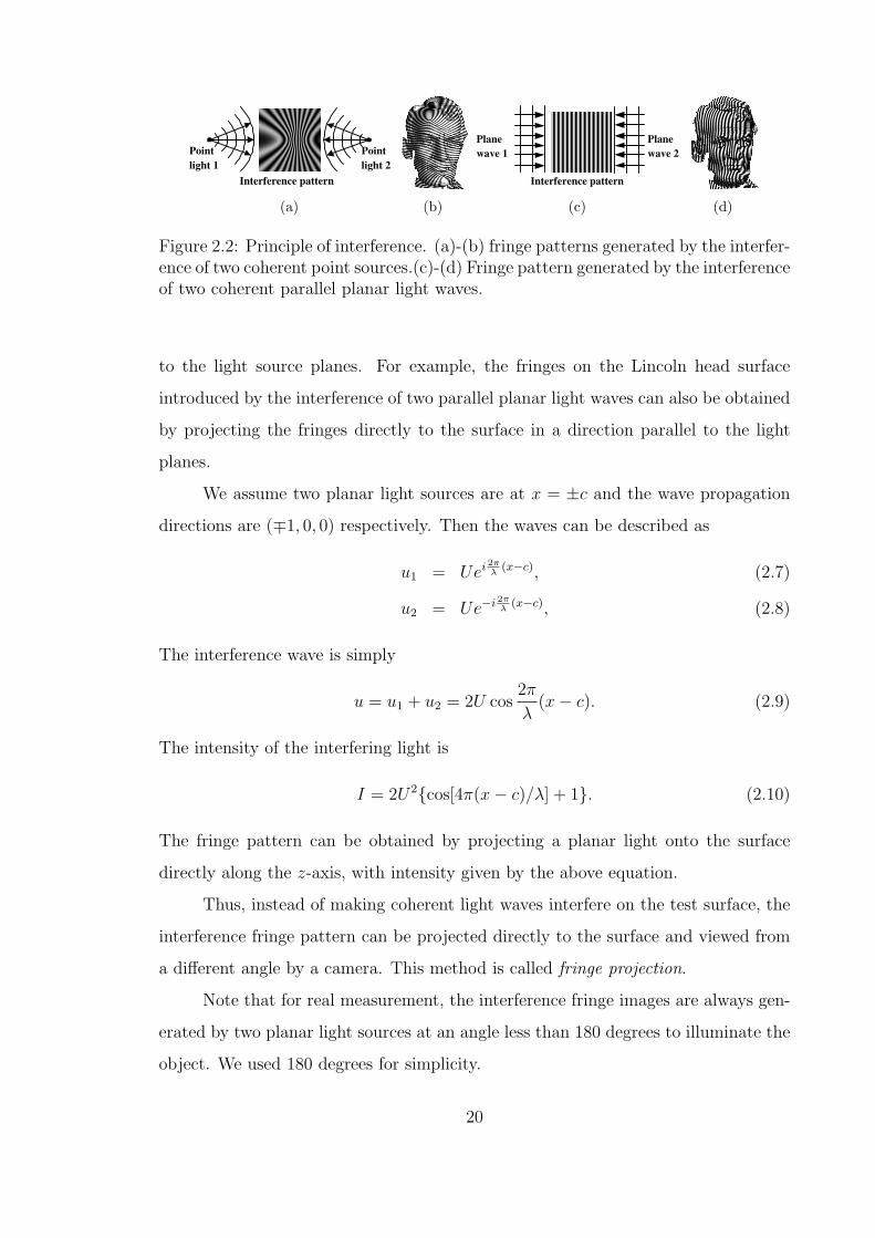
(c) (d)

Figure 2.2: Principle of interference. (a)-(b) fringe patterns generated by the interfer-ence of two coherent point sources.(c)-(d) Fringe pattern generated by the interferenceof two coherent parallel planar light waves.

to the light source planes. For example, the fringes on the Lincoln head surface

introduced by the interference of two parallel planar light waves can also be obtained

by projecting the fringes directly to the surface in a direction parallel to the light

planes.

We assume two planar light sources are at x = ±c and the wave propagation

directions are (∓1, 0, 0) respectively. Then the waves can be described as

u1 = Uei 2πλ

(x−c), (2.7)

u2 = Ue−i 2πλ

(x−c), (2.8)

The interference wave is simply

u = u1 + u2 = 2U cos2π

λ(x− c). (2.9)

The intensity of the interfering light is

I = 2U2{cos[4π(x− c)/λ] + 1}. (2.10)

The fringe pattern can be obtained by projecting a planar light onto the surface

directly along the z-axis, with intensity given by the above equation.

Thus, instead of making coherent light waves interfere on the test surface, the

interference fringe pattern can be projected directly to the surface and viewed from

a different angle by a camera. This method is called fringe projection.

Note that for real measurement, the interference fringe images are always gen-

erated by two planar light sources at an angle less than 180 degrees to illuminate the

object. We used 180 degrees for simplicity.

20

2.2.3 Three-step phase-shifting algorithms

Over the years a number of phase-shifting algorithms have been developed

and applied to real measurement applications, including three-step algorithms, least-

square algorithms etc [68]. All of these algorithms share common characteristics,

they require that a series of fringe images are recorded as the reference phase is

varied. Differences between the various algorithms relate to the number of recorded

fringe images, the phase shift between fringe images, and the susceptibility of the

algorithm to errors in the phase shift or environmental noise such as vibration and

turbulence. This section discusses the three-step phase-shifting algorithm that is

used in this research.

Since there are three unknowns in Equation 2.6, the minimum number of mea-

surements of the fringe images that are required to reconstruct the unknown wave-

front phase is three. Equal phase steps of size α is usually used in the three-step

algorithm. That is

δk = −α, 0, α; k = 1, 2, 3,

and

Ik(x, y) = I ′(x, y) + I ′′(x, y) cos [φ(x, y) + δk] ,

= I ′(x, y) {1 + γ(x, y) cos [φ(x, y) + δk]} , (2.11)

where I ′(x, y) is the average intensity, I ′′(x, y) the intensity modulation or the dy-

namic range of the encoded fringe, and φ(x, y) the phase to be determined, and

γ(x, y) = I ′′(x, y)/I ′(x, y) the data modulation. If phase shift is α = 2π/3, solving

Equations 2.11 gives,

φ(x, y) = tan−1

(√3

I1 − I3

2I2 − I1 − I3

), (2.12)

I ′(x, y) = (I1 + I2 + I3)/3, (2.13)

γ(x, y) =I ′′(x, y)

I ′(x, y)=

√3(I1 − I3)2 + (2I2 − I1 − I3)2

I1 + I2 + I3

. (2.14)

The advantage of this three-step algorithm is that it requires the minimum

number of three fringe patterns, which translates into high speed. The drawback of

21

this algorithm is its sensitivity to errors in the phase shift between frames. However,

a DLP projector is utilized in this research to project computer generated phase-

shifted fringe images, no phase-shift error will be introduced. Therefore, we choose

this three-step phase-shifting algorithm for our real-time 3D shape system.

2.2.4 Phase unwrapping methods

Phase φ(x, y) can be recovered with ambiguity of 2kπ, where k ∈ Z, from

fringe images using Equation 2.12. The discontinuities occur every time φ changes

by 2π. Phase unwrapping aims to unwrap or integrate the phase along a path

counting the 2π discontinuities. The key to reliable phase unwrapping is the ability

to accurately detect the 2π jumps. However, for complex geometric surfaces, noisy

images, and sharp changing surfaces, phase-unwrapping procedure is usually very

difficult. This section introduces four basic phase unwrapping algorithms, namely, the

path integration, spatial coherent, two-wavelength, and interactive phase unwrapping

algorithms.

2.2.4.1 Path integration phase unwrapping

In principle, the 2π phase jump curves are special level sets of the depth func-

tion z(x, y). In general, they are closed curves on the surface, or curves intersecting

the boundaries or shadow or occlusion areas. The self-occlusion area is in general

difficult to locate from phase map. The red curves in the first image in the second

row of Figure 2.3 illustrates the phase jumping curves.

In an ideal noise-free wrapped phase image with adequately sampled data such

that the phase gradients are significantly less than 2π, a simple approach to unwrap

phase is adequate. All that is required is a sequential scan through the object, line

by line, to integrate the phase by adding or subtracting multiples of 2π at the phase

jumps.

Figure 2.3 shows the procedures of path integration phase-unwrapping algo-

rithm. The first row from left to right shows fringe images with −2π/3, 0, 2π/3

phase shift, and wrapped phase map whose value ranges from 0 to 2π. The first

22

Figure 2.3: 3D result by the path integration phase unwrapping method.

image in the second row is the wrapped phase map with areas of 2π phase jumps

detected (indicated in red. The second and last images illustrate the reconstructed

3D geometric model at different view angles. The third image shows the 3D model

with texture mapping. Here the texture image was generated by averaging the three

phase-shifted fringe images.

For most captured images, noise in the sampled data is a major contribut-

ing factor in the false identification of phase jumps. The real phase jumps will be

obscured if the noise amplitude approaches 2π.

2.2.4.2 Spatial coherent phase unwrapping

Assume the wrapped phase is represented as ψ(x, y). The goal is to find a

smooth function φ(x, y) such that the gradient of φ(x, y) approximates the gradient

of ψ(x, y) as closely as possible. Thus we use the following variational approach to

find a continuous function φ(x, y) that minimizes the functional,

J(φ) =

∫ ∫|∇φ−∇ψ|2. (2.15)

23

The Euler-Langrange equation is ∆φ = ∆ψ, where ∆ = ∂2

∂x2 + ∂2

∂y2 . This is a Poisson’s

equation and can be easily solved using either the conjugate gradient method or a

Fast Fourier Transform as in Ref. [69].

The real phase jumps will be obscured in the shadow or near the self-occlusion

area of the projection fringes where the projection light is tangent to the surface.

The quality of each pixel in the wrapped phase map is mainly determined by two

factors, namely, the phase gradient and the visibility. Pixels with low gradient and

high visibility are more reliable. Therefore, we adjust our functional as

J(φ) =

∫ ∫γ

1 + |∇ψ|2 (|∇φ−∇ψ|2). (2.16)

The functional can be converted to a weighted least square problem and solved by

using the conjugate gradient method directly [70].

For surfaces with high continuity and less self-occlusion, the spatial coherent

phase unwrapping algorithm works well. For surfaces with many self-occlusion re-

gions and sharp phase gradient, phase unwrapping is more challenging. In this case,

the two-wavelength phase-unwrapping algorithm can be applied.

2.2.4.3 Two-wavelength phase unwrapping

In order to remove the ambiguity of the phase, one can choose a special projec-

tion fringe such that the wavelength λ is large enough to cover the whole depth range

of the scene. Thus, no phase unwrapping will be necessary at all. Unfortunately, the

cost of increasing the wavelength is the decrease of the quality of the reconstructed

3D data. Therefore, one can capture two sets of fringe images with different wave-

lengths. The first one with a longer wavelength will remove the phase ambiguity

but produce poor result. The second one will produce high quality result, but with

phase ambiguity. Therefore, if we unwrap the second phase map while keeping the

geometric consistency with the first one, we can obtain high quality data without

the problem of phase ambiguity.

Figure 2.4 illustrates an example of 3D reconstruction employing the two-

wavelength phase unwrapping algorithm. The first image is one of the fringe images

24

Figure 2.4: 3D reconstruction by two-wavelength phase-unwrapping algorithm.

with a longer wavelength. The geometry changes are less than 2π. Therefore, 3D

information can be retrieved correctly although the quality is poor. The third image

shows one of the fringe images with a shorter wavelength and the geometric changes

are beyond 2π somewhere on the surface. Thus phase unwrapping cannot correctly

reconstruct the geometry as illustrated in the fourth image. But with the reference

of geometric information reconstructed with the longer wavelength fringe images as

references, 3D shape can be correctly reconstructed as shown in the last image.

However, there are still some limitations for this method. The 2π phase am-

biguity of the second phase map must be less than the phase error caused by the

discretization error of the first phase map. Assume that the wavelengths are λ1, λ2,

and the number of bits for each pixel is n, then

λ1

λ2

< 2n.

If the depth range of the scene is very large, and the reconstructed geometry is

required to be of high quality, then one can apply the multiple-wavelength phase-

unwrapping algorithms.

The two-wavelength method is undesirable for high-speed data acquisition ap-

plications because it reduces the acquisition speed by half, but it is preferable for

measuring static objects, especially those that would result in self-occlusions in the

phase image.

25

2.2.4.4 Interactive phase unwrapping

For those systems that do not allow taking more images, such as our real-time

system, the reconstruction procedure may require manual work. In this research, we

develop an interactive Graphic User’s Interface (GUI) tool that allows the user to

correct those areas that have not been correctly unwrapped.

Users have the most accurate information about the quality of the reconstructed

result. Therefore, if the user can communicate with the computer, providing feedback

of the reconstruction result, the final phase unwrapping result will be satisfactory.

In this research, we develop a GUI that allows the users to perform interactive phase

unwrapping. Figure 2.5 shows the software interface of the GUI tool. The basic

idea behind this tool is that the user tells the algorithm where two regions should

separate. The underline phase-unwrapping algorithm is a simple path integration

method. Figure 2.6 shows an example. The direct phase unwrapping resulted in

geometric jumps. These jumps are due to the geometric changes beyond 2π around

the regions of the little horse’s mouth and the mother horse’s tail. Pre-knowledge

tells us that the small horse head should be separate with other areas, therefore

we draw a spline (illustrated in the third image of Figure 2.6). This line tells the

algorithm not to cross the line. Similarly, we draw another spline at the back. After

being given these additional information, the algorithm can correctly reconstruct the

3D information of this sculpture. This special case cannot be correctly reconstructed

using other algorithms without an increase in the number of fringe images. Moreover,

this tool runs very fast. It can reconstruct a 3D model and render it in less than 12.5

ms, therefore the user can interactively view the effect of the operations.

2.3 Typical 3D Shape Measurement System Setup

A simple approach for 3D shape measurement is to project fringe or a grating

onto an object and then view it from another direction. The deformation of the

projected fringes by the object provides the information to reconstruct the shape of

the 3D object.

The fringe pattern can be generated by a personal computer, projected by

26

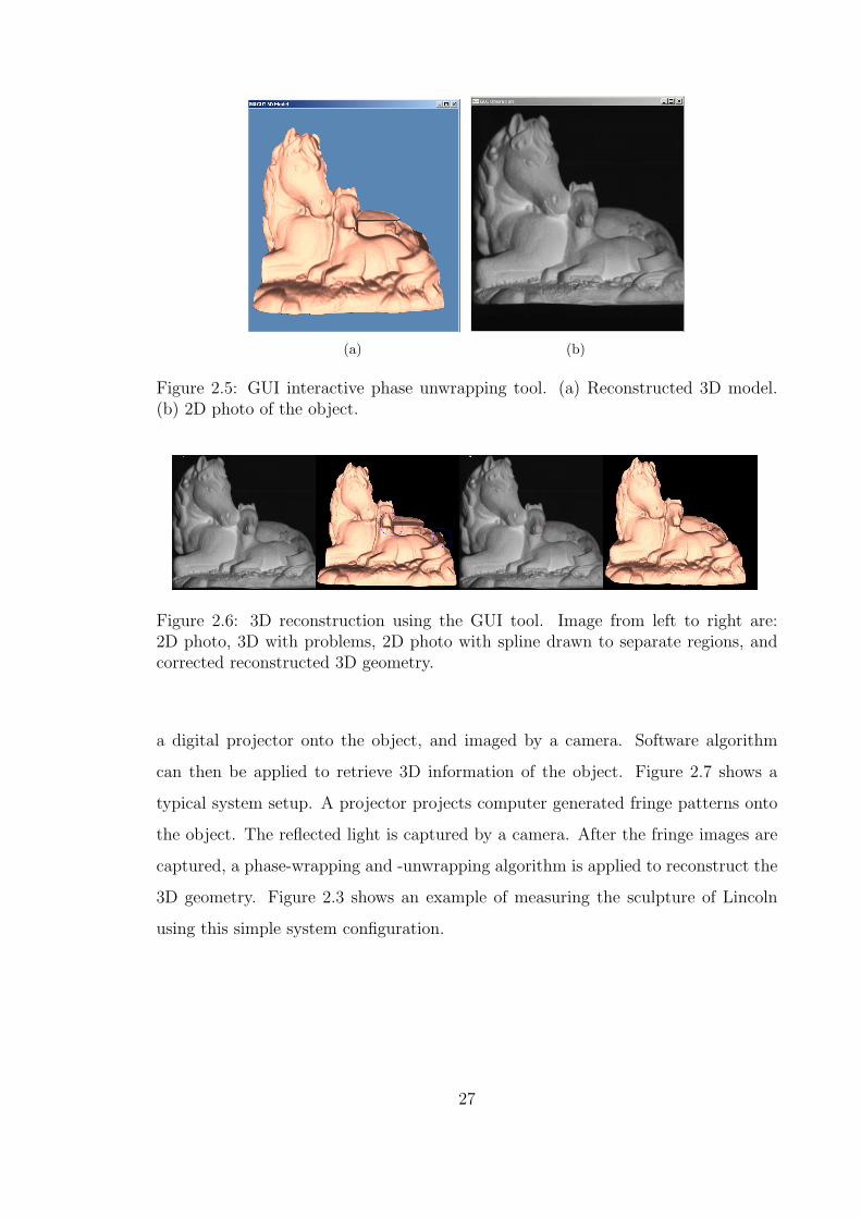
(a) (b)

Figure 2.5: GUI interactive phase unwrapping tool. (a) Reconstructed 3D model.(b) 2D photo of the object.

Figure 2.6: 3D reconstruction using the GUI tool. Image from left to right are:2D photo, 3D with problems, 2D photo with spline drawn to separate regions, andcorrected reconstructed 3D geometry.

a digital projector onto the object, and imaged by a camera. Software algorithm

can then be applied to retrieve 3D information of the object. Figure 2.7 shows a

typical system setup. A projector projects computer generated fringe patterns onto

the object. The reflected light is captured by a camera. After the fringe images are

captured, a phase-wrapping and -unwrapping algorithm is applied to reconstruct the

3D geometry. Figure 2.3 shows an example of measuring the sculpture of Lincoln

using this simple system configuration.

27

Figure 2.7: Typical 3D shape measurement system setup.

2.4 Summary

This chapter introduced the DLP digital projection display technology, re-

viewed three-step phase-shifting algorithm and phase-unwrapping algorithms, and

finally described a basic 3D measurement system based on a digital fringe projection

technique.

28

Chapter 3

High-resolution, Real-time 3D Shape Measurement System

This chapter describes a high-resolution, real-time 3D shape measurement sys-

tem developed in this research. The system is based on a digital fringe projection and

phase shifting technique. It utilizes a single-chip DLP projector to project computer

generated fringe patterns to the object and a high-speed CCD camera synchronized

with the projector to acquire the fringe images at a frame rate of 120 frames per

second. Based on a three-step phase-shifting technique, each frame of the 3D shape

of the object is reconstructed using three consecutive fringe images. A color CCD

camera is also used to capture color images for color texture mapping. By imple-

menting a novel fast phase-wrapping algorithm and parallel processing technique, we

realize simultaneous 3-D data acquisition, reconstruction, and display at a frame rate

of up to 40 frames per second and a resolution of 532× 500 points per frame.

3.1 Introduction

To achieve real-time 3D measurement, there are basically two approaches: one

is to use a single pattern (typically a color pattern), the other method is use multiple

patterns and switch them rapidly so that images required for reconstructing the 3D

geometry can be captured in a short period of time. In this research, we adopted

the second approach. Three phase-shifted fringe patterns are encoded in the three

primary color channels and projected by a single-chip DLP projector in sequence at

a frame rate of 80 Hz. A properly synchronized high-speed B/W CCD camera is

used to capture the distorted fringe patterns in real time. In order to achieve more

29

realistic visual effect, a color camera synchronized with the B/W camera is used to

provide color images for texture mapping.

The rest of this chapter is organized as follows. Section 3.2 explains the basic

principle of this high-resolution, high-speed 3D shape measurement system. Sec-

tion 3.3 introduces the system setup. Section 3.4 describes a system that is able to

capture color photo simultaneously. Section 3.5 introduces a new system that gives

high quality data stably. Section 3.6 presents the framework of simultaneously data

acquisition, reconstruction and display. Section 3.7 discusses the advantages and

disadvantages of this real-time system. And Section 3.8 summarizes the chapter.

3.2 Principle

3.2.1 Projection mechanism of a single-chip DLP projector

One of the keys to successfully developing this real-time system is to under-

stand the projection mechanism of a single-chip DLP projector. In this research,

a commercial Kodak DP900 projector is extensively studied. For the DLP projec-

tor, a photodiode behind the color wheel supplies a trigger signal to the DMD to

generate images. However, since color is not desired in this research, the color fil-

ters are removed. As a result, the photo sensor cannot detect the color signal and

supply the trigger signal to DMD, which disables the projector from projecting im-

ages. Figure 3.1(a) shows the position of the photo-detector, Figure 3.1(b) shows the

commercial projector with the color filters while Figure 3.1(c) shows the modified

projector without the color filters. To make the projector work without the color

filters, Zhang found an approach by supplying the projector with an externally gen-

erated 2-level current signal to replace the trigger signal from the photo sensor [71].

Some experiments were done and reasonable results were obtained.

However, in this research, we find that the projector could not work stably if

it is triggered by the 2-level current signal. After operating for a while, the projector

flashes and starts to project images improperly. To improve the stability of the

projector, a parallel input 12-bit D/A converter is utilized to generate a 2-level

voltage signal, 10 mv at the low level and 56 mv at the high level, respectively. We

30

Photo-detector

(a)

Color wheel

(b) (c)

Figure 3.1: DLP projector and color filters. (a) Projector with photo sensor. (b)Projector with color filters. (c) Projector without color filters.

also notice that the projector always starts projecting images at the falling edge of the

trigger signal and projects red, clear (white), green, and blue channels sequentially

when the trigger signal has a period longer than 10 ms. After repeated experiments,

we find the optimal trigger signal period to be 12.5 ms, at which the projector works

most stably.

3.2.2 System synchronization

After fully understanding the projection mechanism of the single-chip DLP

projector, it is possible to take advantage of it to boost the 3D measurement speed.

Three phase-shifted fringe images are encoded in three the primary color channels

(RGB) of the projector. Since the color filters are removed, the projector projects

three phase-shifted gray scale fringe images sequentially and repeatedly at a high

speed when the RGB fringe image is sent to the projector. If a high-speed camera

synchronized with the projector is used, three fringe images can be captured rapidly

for real-time 3D shape measurement.

Figure 3.2 shows the timing chart of our system. The waveform at the top

is the trigger signal to the projector. The projector’s trigger signal is generated by

an external micro-controller based timing signal circuit. The internal timing signal

of the projector is disabled. The middle waveform is the projection timing chart,

where R, G, B, and C represent the red, green, blue, and clear channels of the

projector. The clear channel is designed to enhance the brightness of the projected

image. The projection signal shows the sequence and timing of the color channels.

31

Trigger to projector

Projected signal

Trigger to camera

Cycle time (12.5 ms)

Exp. R Exp. B Exp. G

2.8ms 2.6ms 2.5ms

R GC B R GC B

Figure 3.2: System timing chart.

The projection cycle starts with the red channel at the falling edge of the projector

trigger signal. The bottom waveform is the trigger signal to the B/W CCD camera.

The camera’s trigger signal is generated by the same micro-controller based circuit,

which guarantees its synchronization with the projector’s trigger signal. Because of

the limitation of the frame rate of our camera (maximum of 262 frames per second),

two cycles of projection are needed for the camera to capture the three phase-shifted

fringe patterns, which results in a frame rate of 40 frames per second for 3D data

acquisition. If a higher speed camera is used, a maximum frame rate of 80 Hz can

be achieved.

The non-uniform distribution of three color channels of the projector can po-

tentially affect the measurement accuracy. We observe that the RGB channels do

not have the same duration time (red is approximately 2.8 ms and blue is approx-

imately 2.5 ms). For this real-time system, the exposure time of the camera could

not be adjusted according to each individual frame. To solve this problem, we set

the exposure time at a fixed time of 2.8 ms for all channels and take advantage of the

0.2 ms gaps between channels to make sure that all channels are captured properly,

as shown in Figure 3.3. One should notice that with this timing design, only the red

channel is truly synchronized. The green and blue channels are pseudo synchronized.

3.2.3 Color-encoded three-step phase-shifting algorithm

As introduced in Chapter 2, three-step phase-shifting algorithm requires min-

imum number of fringe images to reconstruct 3D shape. In general, the three color

encoded fringe images with a phase shift of 2π/3 generated by a computer are, re-

32

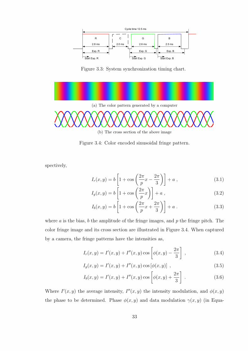
R C G B

2.8 ms 2.0 ms 2.6 ms 2.5 ms

Cycle time 12.5 ms

Exp. BExp. R Exp. G

Start Exp. BStart Exp. GStart Exp. R

Figure 3.3: System synchronization timing chart.

(a) The color pattern generated by a computer

(b) The cross section of the above image

Figure 3.4: Color encoded sinusoidal fringe pattern.

spectively,

Ir(x, y) = b

[1 + cos

(2π

px− 2π

3

)]+ a , (3.1)

Ig(x, y) = b

[1 + cos

(2π

px

)]+ a , (3.2)

Ib(x, y) = b

[1 + cos

(2π

px +

2π

3

)]+ a . (3.3)

where a is the bias, b the amplitude of the fringe images, and p the fringe pitch. The

color fringe image and its cross section are illustrated in Figure 3.4. When captured

by a camera, the fringe patterns have the intensities as,

Ir(x, y) = I ′(x, y) + I ′′(x, y) cos

[φ(x, y)− 2π

3

], (3.4)

Ig(x, y) = I ′(x, y) + I ′′(x, y) cos [φ(x, y)] , (3.5)

Ib(x, y) = I ′(x, y) + I ′′(x, y) cos

[φ(x, y) +

2π

3

]. (3.6)

Where I ′(x, y) the average intensity, I ′′(x, y) the intensity modulation, and φ(x, y)

the phase to be determined. Phase φ(x, y) and data modulation γ(x, y) (in Equa-

33

tions 2.12 and 2.14) respectively become,

φ(x, y) = arctan

(√3

Ir − Ib

2Ig − Ir − Ib

), (3.7)

and

γ(x, y) =I ′′(x, y)

I ′(x, y)=

√3 (Ir − Ib)

2 + (2Ig − Ir − Ib)2

Ir + Ig + Ib

. (3.8)

A phase map with the phase ranging from 0 to 2π is obtained after this step. A

continuous phase map can be obtained by phase unwrapping (see Section 2.2.4).

3.2.4 Projection nonlinearity correction

The accuracy of the phase measurement can be improved by reducing sys-

tematic errors of the system. In phase shifting interferometry [72], the most com-

mon sources of systematic errors include nonsinusoidal waveforms of a signal due

to multiple-beam interference or nonlinearity of the detector and phase-shift errors

due to a miscalibration or nonlinear projection response of the phase shifter. In our

system, the dominant error source is nonsinusoidal waveforms due to the nonlinear

projection curve (or gamma curve) of the projector. This nonlinear projection re-

sponse makes the intensity profile of the fringe images nonsinusoidal and therefore

causes phase measurement errors. Phase shifting error in our system is negligible

because of the digital nature of the fringe generation technique.

The projection response curve of a commercial video projector, which repre-

sents the relationship between the input gray scale values generated by the computer

and the output intensity values projected by the projector and captured by the cam-

era, is typically designed to be nonlinear for better visual effects. Figure 3.5(a) shows

a typical projection response curves of the Kodak DP900 projector obtained experi-

mentally. The projected intensity is measured by the CCD camera. Notice that when

the input gray scale value is less than approximately 45, the projected intensity value

almost does not change. This part of the input gray scale value is therefore not used

in our experiment. In our experiment, we adjust the brightness, contrast, and tint

of the projector to make the projection response curves for the three color channels

34

0 50 100 150 200 2500

50

100

150

200

250

Projetor input grayscale values

Cam

era

capt

ured

gra

ysca

le v

alue

s

RGBIdeal

(a)

0 50 100 150 200 2500

50

100

150

200

250

Projetor input grayscale values

Cam

era

capt

ured

gra

ysca

le v

alue

s

RGBIdeal

(b)

Figure 3.5: System projection response curve. (a) The curves before nonlinearitycompensation. (b)The curves after compensation.

to be as close to each other as possible and their nonlinearity as small as possible

before nonlinearity correction is performed.

To compensate for the nonlinearity of the projector, the projection response

curves are fitted with spline, whose inverse functions are then used to modify the

input gray scale values of the fringe images generated by the computer. Figure 3.5(b)

shows the projection response curves after nonlinearity correction, which are almost

linear.

This method provides fairly good measurement accuracy, however, the short-

coming is obvious. However, no matter how careful the calibration is done, the

projection response curve could never be truly linear, which causes residue errors. In

Chapter 6, we will discuss another error compensation method that further improves

the accuracy.

3.2.5 Coordinate conversion

The measured phase contains the height information of the measured object,

which can be extracted by using a phase-to-height conversion algorithm. Since in this

real-time system, we are more interested in the relative height variations on an object

surface than absolute coordinates, a simple approximate approach by subtracting

reference plane is employed [48].

35

In order to covert phase to height, the relationship between the height and

phase has to be established. The schematic diagram of the system is illustrated in

Figure 3.6. Points P and I are the center of the exit pupil of the DLP projector

and that of the CCD camera, respectively. The optical axes of the projector and

the camera coincide at point O. After the system has been set up, a flat reference

plane is measured first whose phase map is used as the reference for subsequent

measurements. The height of the object surface is measured relative to this plane.

From the point view of the DMD camera, point D on the object surface has the

same phase value as point C on the reference plane, φD = φC . While on the CCD

array, point D on the object surface and A on the reference plane are imaged on the

same pixel. By subtracting the reference phase map from the object phase map, we

obtained the phase difference at this specific pixel:

φAD = φAC = φA − φC , (3.9)

Assume points P and I are designed to be on the same plane with a distance l to

the reference plane and have a fixed distance d between them, and reference plane is

parallel to the device. Thus, 4PID and 4CAD are similar, the height of point D

on the object surface relative to reference plane DB can be related to the distance

between points A and C, or AC:

d

AC=

l −DB

DB=

l

DB− 1 , (3.10)

Since d is much larger than AC for real measurement, this equation can be simplified

as

z(x, y) = DB ≈ l

dAC =

pl

2πdφAC = KφAC , (3.11)

where p is the fringe pitch on the reference plane. Therefore, a proportional relation-

ship between the phase map and the surface height can be derived.

A calibration standard with a known height is used to determine the phase-

height conversion constant K. The calibration height of the step from the flat board

is 1.506± 0.01 inches. Figure 3.7 shows a measurement result of a flat board with a

step height on top. From the cross section of the top surface and bottom surfaces, we

36

BA CO

I

l

DMD CCDd

D

P

Reference Plane

Object

Figure 3.6: Schematic diagram of phase-to-height conversion.

can calculate the phase difference between the top and bottom surfaces of the step

is φAC = φA− φC = φtop− φbottom = 3.6054− (−0.9909) = 4.5963 rad. Therefore the

constant K is:

K =1.506

4.5963= 0.3227(inch/rad) = 8.3224(mm/rad) . (3.12)

We assume the x and y coordinate values are proportional to the real coordinate

of the object for this simple algorithm. The measured area on the reference plane is

260 × 244 mm, therefore, the x and y coordinate conversion constants are,

kx = ky =260

532= 0.4887(mm/pixel) . (3.13)

By applying K, kx and ky on the 3D phase map of the reconstructed image, we can

obtain the 3D coordinates of the measured object.

This calibration method only gives approximate relationship between the phase

map and the real coordinates. For objects with small depth, all assumptions can be

sufficiently satisfied. However, for objects with large depths, this simple calibration

may not provide accurate results for the following reasons:

(1) The reference plane is required to put parallel to the device. It is difficult

for practice to measure the reference plane.

(2) The fringe is assumed to be uniformly distributed on the reference plane. It

is usually not the case.

37

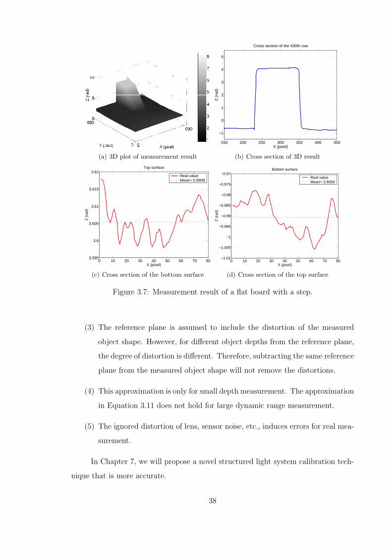
(a) 3D plot of measurement result

150 200 250 300 350 400 450

−1

0

1

2

3

4

5

X (pixel)

Z (

rad)

Cross section of the 430th row

(b) Cross section of 3D result

0 10 20 30 40 50 60 70 803.595

3.6

3.605

3.61

3.615

3.62

X (pixel)

Z (

rad)

Top surface

Real valueMean= 0.9909

(c) Cross section of the bottom surface

0 10 20 30 40 50 60 70 80−1.01

−1.005

−1

−0.995

−0.99

−0.985

−0.98

−0.975

−0.97

X (pixel)

Z (

rad)

Bottom surface

Real valueMean= 3.6054

(d) Cross section of the top surface

Figure 3.7: Measurement result of a flat board with a step.

(3) The reference plane is assumed to include the distortion of the measured

object shape. However, for different object depths from the reference plane,

the degree of distortion is different. Therefore, subtracting the same reference

plane from the measured object shape will not remove the distortions.

(4) This approximation is only for small depth measurement. The approximation

in Equation 3.11 does not hold for large dynamic range measurement.

(5) The ignored distortion of lens, sensor noise, etc., induces errors for real mea-

surement.

In Chapter 7, we will propose a novel structured light system calibration tech-

nique that is more accurate.

38

Wrapped

phase map

DLP

projector

PC2

RGB

fringe

Object

RS232

PC1

B/W CCD

camera

3D W/

Texture

G

(0 o ) R

(-120 o )

B

(120 o )

R

G

B

I 1

I 2

I 3

3D

model

2D

photo

Figure 3.8: Schematic diagram of the real-time 3D shape measurement system.

3.3 Real-time 3D Shape Measurement System

3.3.1 System setup

Figure 3.8 shows the schematic diagram of the real-time 3D shape measurement

system developed in this research. A color fringe pattern is generated by a Personal

Computer (PC) and is projected onto the object by a DLP video projector (Kodak

DP900). A high-speed B/W CCD camera (Dalsa CA-D6-0512W) synchronized with

the projector is used to capture the distorted fringe images of each color channel.

Phase-wrapping and -unwrapping algorithms are implemented to reconstruct the 3D

geometry. Since the fringe images used have 2π/3 of phase shift, averaging three

fringe images result in a 2D image without fringes, which can be used for texture

mapping. Figure 3.9 is a picture of the system developed in this research.

The whole measurement system basically includes five components: one Dell

desktop computer (Pentium 4, 2.8 GHz CPU, 1 GB DDR SDRAM at 333 MHz, 80

GB hard drive) with a Matrox frame grabber Meteor II/Digital installed, one Kodak

DP900 digital projector, one Dalsa high-speed CCD camera (CA-D6-0512), and one

external timing signal generator circuit board.

39

Projector

Timing signal generator circuit

Power supply

CCD camera

Figure 3.9: Photograph of the real-time 3D shape measurement system.

The digital projector has one DMD chip with a resolution of 800 × 600 pixels

and a brightness of 900 lumens. It receives the video signal from a PC’s video output

and projects the image onto the object surface.

The CCD camera is a high-speed camera with full frame rate at 262 frames per

second. It has 532(H) × 516(V) pixels CCD image sensor with 10 mm square pixels

with 100% fill factor, and 8-bit data depth (256 gray levels).

In this research, we use Matrox frame grabber, which supports digital video

acquisition from standard and non-standard cameras in a single or multi-tap con-

figuration, offering RGB and monochrome grabs. There are some different software

tools that support the frame grabber. In this research, the Matrox Imaging Library

(MIL) provided by Matrox imaging is used, which is basically a set of functions that

controls image acquisition, transferring, displaying and processing.

Figure 3.10 is the schematic diagram of the timing signal generator circuit that

provides the signals to trigger projector as well as the camera. The trigger signal to

the projector is voltage signal +10 mv at low level and +56 mv at the high level,

The trigger signal for the camera is an opto-isolated differential signal connected to

the frame grabber via RS232. The exposure time can be adjusted by the user.

In order to capture 120 2D 8-bit fringe images per second, a software algo-

40

AT89C52

EIA/TTL

Converter

DAC

Output to DP900 projector

56mv

10mv

5v

Output to CCD camera

Figure 3.10: Schematic diagram of the timing signal generator circuit.

rithm called “double buffering” is utilized. The principle of double buffering is that

the events of grabbing and transferring images occur simultaneously under the asyn-

chronous mode of the camera. A parallel software is developed to acquire a large

number of images continuously.

Image acquisition is the first step. The second step is to utilize the 3D vision

software developed in this research to reconstruct 3D models. OpenGL tools are

employed to render the 3D model, GLUT is utilized to create the GUI. Figure 3.11

shows the modules of our 3D Vision software, which consists of eight modules in-

cluding fringe generation, image capture, camera control, phase wrapping, phase

unwrapping, coordinate calculation, 3D display, and file I/O. Fringe generation is

responsible for producing various types of fringe patterns with shifted phases. Image

acquisition controls real-time image data acquisition. Phase wrapping and unwrap-

ping modules include algorithms for image processing and 3D model reconstruction.

Coordinate calculation module is used to calculate the real x, y and z coordinates

from the phase map. 3D display is used to render the measured results, while the

File I/O module handles various data preprocessing, data storing, data converting,

and data saving.

3.3.2 Experiments

After calibration, we first tested the measurement uncertainty of the system.

Figure 3.12 shows the measured results of a flat board. Since the surface is very

smooth, the variations shown in the results are largely due to the noise of the system,

which is RMS 0.05 mm for the measured area. We then measured a static sculpture,

the results are shown in Figure 3.13. The geometric result is shown in Figure 3.13(d),

41

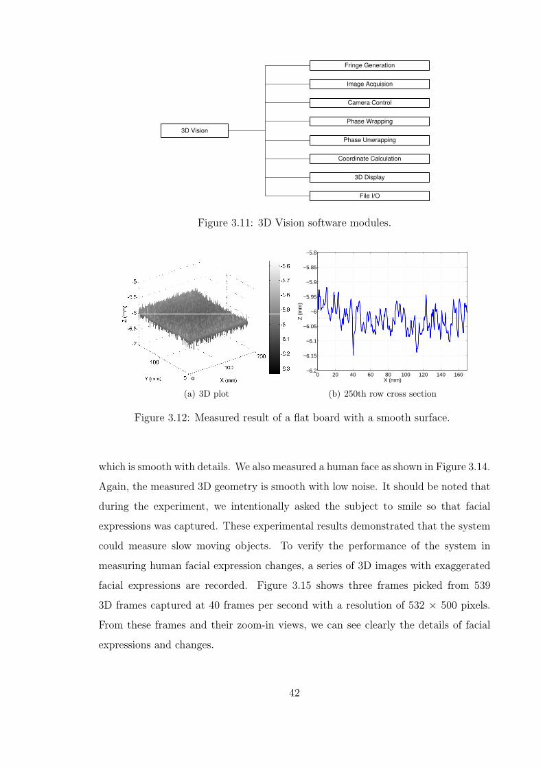
Fringe Generation

Image Acquision

Camera Control

Phase Wrapping

Phase Unwrapping

Coordinate Calculation

3D Display

File I/O

3D Vision

Figure 3.11: 3D Vision software modules.

(a) 3D plot

0 20 40 60 80 100 120 140 160−6.2

−6.15

−6.1

−6.05

−6

−5.95

−5.9

−5.85

−5.8

X (mm)

Z (

mm

)

(b) 250th row cross section

Figure 3.12: Measured result of a flat board with a smooth surface.

which is smooth with details. We also measured a human face as shown in Figure 3.14.

Again, the measured 3D geometry is smooth with low noise. It should be noted that

during the experiment, we intentionally asked the subject to smile so that facial

expressions was captured. These experimental results demonstrated that the system

could measure slow moving objects. To verify the performance of the system in

measuring human facial expression changes, a series of 3D images with exaggerated

facial expressions are recorded. Figure 3.15 shows three frames picked from 539

3D frames captured at 40 frames per second with a resolution of 532 × 500 pixels.

From these frames and their zoom-in views, we can see clearly the details of facial

expressions and changes.

42

(a) (b) (c) (d) (e)

Figure 3.13: 3D shape measurement results of the sculpture Sapho. (a) I1(−2π/3).(b) I2(0). (c) I3(2π/3). (d) 3D geometry. (e) 3D geometry with texture mapping.

(a) (b) (c) (d) (e)

Figure 3.14: 3D shape measurement result of a human face. (a) I1(−2π/3). (b)I2(0). (c) I3(2π/3). (d) 3D geometry. (e) 3D geometry with texture mapping.

3.4 System with Color Texture Mapping

Color texture mapping is desired for many applications. However, for 3D data

acquisition, color should be avoided because it affects the measurement accuracy.

In order to solve this dilemma, we develop a system with two cameras: A B/W

camera and a color camera. The B/W camera is used to capture fringe images for

3D geometric reconstruction, and the color camera is used to provide color photos

for color texture mapping.

3.4.1 System setup

Figure 3.16 illustrates the schematic diagram of the real-time 3D shape mea-

surement system with color texture mapping. A color camera (Uniq Vision UC-930)

43

Figure 3.15: Measurement results of human facial expressions.

synchronized with the projector is added in the previously developed B/W system

shown in Figure 3.8. A beam splitter is used to divide the incoming light into two

parts, one for the B/W camera, and the other for the color camera. Since the

transmitted portion and reflected part are from the same input light source, viewing

from both directions gives the same information excluding the difference of intensity.

44

Wrappedphase map

3D shape

DLPprojector

PC2

RGBfringe

Object

RS232

PC1

B/W camera

Color camera 3D color2D color

photo

Beam splitter

G(0o)R

(-120o)

B(120o)

R

G

B

I1

I2

I3

Figure 3.16: Schematic diagram of the real-time 3D shape measurement system withcolor texture mapping.

Therefore, the color photo acquired by the color camera can be used for texture

mapping purpose.

The color camera is a 10-bit pseudo-color camera using a Bayer color filter. The

color information is recorded in a single sensor simultaneously. The indices of the

pixels are encoded to certain standard that indicates which color the pixel represents.

The color information can be recovered by software from the single image.

3.4.2 Camera synchronization

The exposure time of the color camera is chosen to be one projection cycle, 12.5

ms, to eliminate the fringe pattern and produce the texture image. Figure 3.17(a)

shows the timing chart of the color system. The waveform at the top is the trigger

signal to the projector generated by a microcontroller based timing signal circuit. The

second waveform from the top is the projection timing chart. The next two waveforms

are the trigger signals to the B/W camera and the color camera, respectively. The

frame rate for the color camera is limited to 26.7 frames per second, which is good

enough for texture mapping purpose. In order to keep color and B/W cameras

synchronized, we reduce the frame rate of our 3D acquisition so that it is the same as

that of the color camera. However, the time for acquiring three phase-shifted fringe

patterns is kept the same. Therefore, potential object motion induced error will stay

45

Cycle time (12.5 ms) Trigger to projector

Exp. R Exp. B Exp. G

2.8ms 2.6ms 2.5ms

Exp. color camera

Projected signal

Trigger to B/W camera

Trigger to color camera

R GC B R GC B R GC B

(a)

Cycle time (12.5 ms) Trigger to projector

Exp. R Exp. B Exp. G

2.8ms 2.6ms 2.5ms

Exp. color camera (12.5 ms)

Projection timing

Trigger to B/W camera

Trigger to color camera

R GC B R GC B R GC B

Cycle time for 3D shape acquisition (25.0 ms)

Cycle time for color camera (37.5ms)

(b)

Figure 3.17: Color system timing chart.

the same. We first use one PC to capture both color and B/W images. To avoid

the conflict of two cameras, a parallel processing software is developed. Figure 3.18

shows a photograph of the developed hardware system with an added color camera.

However, our experiments demonstrate that using one PC to capture images for both

cameras cause large error due to mutual interference. Therefore, instead of one PC,

two PCs are utilized to avoid the interference problem of two cameras. The frame

rate of the B/W camera can remain to be 40 frames per second. The color camera

captures color texture images at a frame rate of 26.7 frames per second. The color

texture images for 3D models in between can be obtained by linearly interpolating

two neighboring images. The timing chart is shown in Figure 3.17(b).

46

Projector

Power supply

Color camera

Timing signal circuit

Beam splitter

B/W camera

Figure 3.18: Photograph of the real-time 3D shape measurement system with colortexture mapping.

3.4.3 Camera alignment

Theoretically, two cameras capture the same images, however, practically, it is

difficult. Therefore aligning two cameras and matching correspondence are necessary.

In order to find the relationship between two cameras, a coordinate transformation

matrix P has to be determined, which satisfies

sxbw

sybw

s

=

p11 p12 p13

p21 p22 p23

p31 p32 p33

xc

yc

1

= PXc, (3.14)

where xbw, ybw are coordinates of the B/W camera, xc, yc coordinates of the color cam-

era, and s the scaling factor. The transformation matrix can be obtained by finding

a set of corresponding points in the B/W image and color image using singular value

decomposition (SVD) algorithm. It should be noticed that the transformation ma-

trix P only needs to be determined once since the relationship between two cameras

is fixed by the hardware system setup.

47

(a) Measured 3D models

(b) Measured results with color texture mapping of the above 3D models

Figure 3.19: Real-time 3D measurement result of human facial expression with colortexture mapping.

3.4.4 Experiments

After the system is calibrated and two cameras are aligned, we measured dy-

namic objects. Again human facial expression was measured. Figure 3.19 are several

frames chosen from a sequence of 540 frames captured at 40 Hz for the 3D model,

and 26.7 Hz for the color texture. We see that the facial expression details were

clearly captured, and that the color texture images are well aligned with 3D geomet-

ric models.

3.5 Real-time 3D Shape Measurement System: Generation II

The Kodak DP900 projector as an early model of DLP projectors, caused many

problems in our system. First, the lamp life span was very short, only 100 hours for

48

Camera Projector

Figure 3.20: Photograph of real-time 3D shape acquisition system: Gen II.

reasonable measurements. Second, the calibration was tedious. It took about one

hour each time to warm up and calibrate the system. Third, the projector was not

stable, with the noise level changing from frame to frame. This is not desirable

for real-time 3D shape measurement. Moreover, the projector has to be shut down

for cooling after working for about 2.5 hours, and thus it is difficult to collect a

large volume of data. Therefore, replacing the projector with a newer model was

necessary. A customized new projector, PLUS U2-1200 was chosen as a substitute.

After replacing the projector, the system became much more stable and easier to

calibrate. Moreover, the projector also has a desirable B/W projection mode that is

convenient for out application. Figure 3.20 shows the developed new system, which

is a little smaller than the old one. But the color camera cannot added due to the

use of a the new DMD projection mechanism in the new projector. The size of the

system is approximately 21′′×12.5′′×10′′. The drawback of the new system is that its

acquisition speed is reduced to 30 frames per second due to the hardware limitation.

Figure 3.21 shows some sculptures measured by the new system. We also

measured dynamic facial expressions as shown in Figure 3.22. 12 frames for this

subject are selected from 539 frames recorded at 30 frames per second. All these

frames have similar noise level, which is good for repeated measurements.

49

Figure 3.21: Measurement results using the new system. From left to right areLincoln, Zeus, Angel, and Horses.

3.6 Real-time 3D Data Acquisition, Reconstruction, and Display

System

The system we developed could acquire 3D data in real time. Our goal was to

achieve simultaneous 3D data acquisition, reconstruction, and display, all in real time.

To reach our goal, a parallel processing software employing a fast 3D reconstruction

algorithm is developed. We will discuss the fast 3D reconstruction algorithms in

Chapters 4 and 5. This section discusses the framework of this real-time system.

3.6.1 Principle

Figure 3.23 illustrates the pipeline of real-time 3D acquisition, reconstruction,

and rendering system. The system includes three threads,

• Acquisition. A high-speed CCD camera captures fringe images in real time,

and the fringe images are continuously sent to the computer.

• Reconstruction. 3D reconstruction algorithm based on newly proposed fast

phase-wrapping algorithm (to be discussed in Chapter 5) is employed to

generate 3D models in real time.

• Display. The 3D models are sent to the graphics card for display.

As discussed above, the new system is able to acquire 90 frames of 2D fringe

images per second. These 2D images are then sent to the computer directly without

50

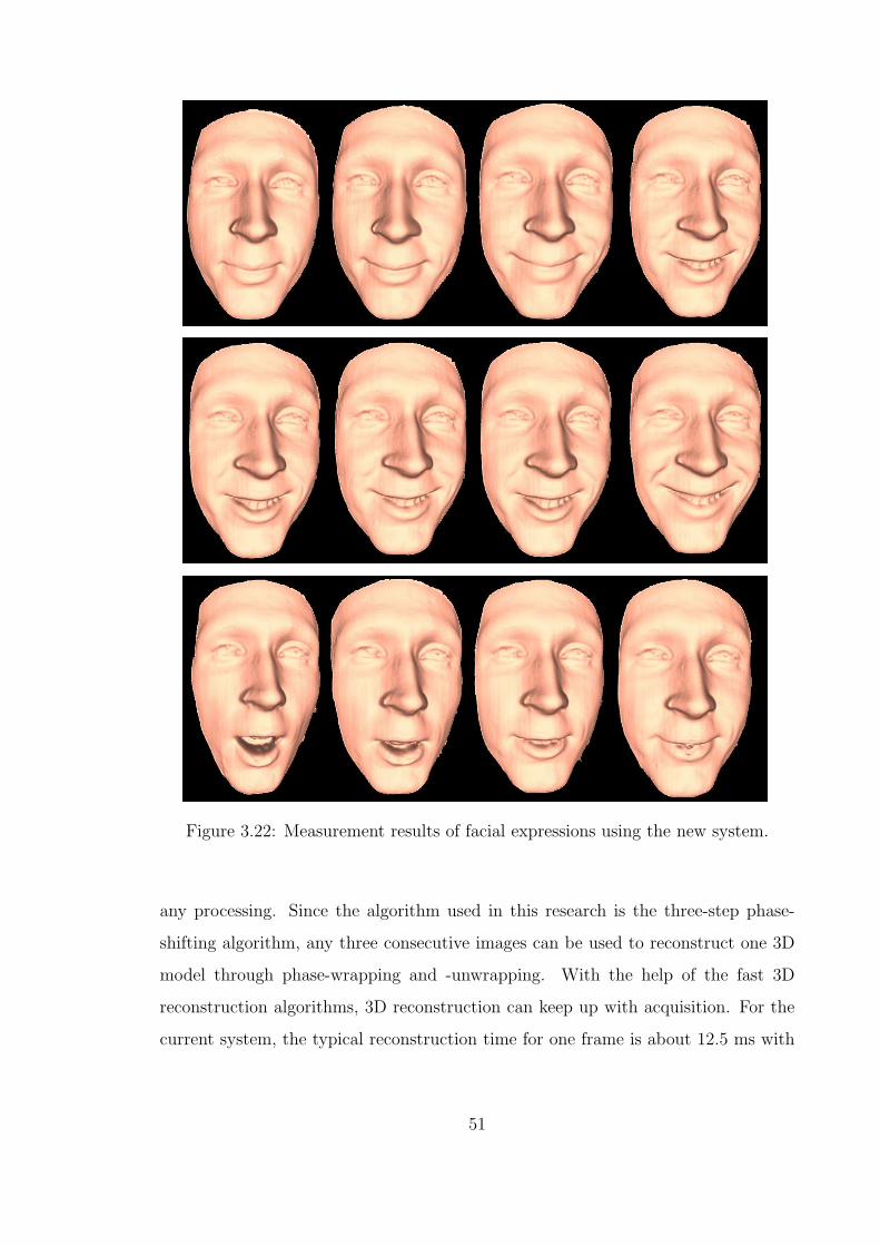
Figure 3.22: Measurement results of facial expressions using the new system.

any processing. Since the algorithm used in this research is the three-step phase-

shifting algorithm, any three consecutive images can be used to reconstruct one 3D

model through phase-wrapping and -unwrapping. With the help of the fast 3D

reconstruction algorithms, 3D reconstruction can keep up with acquisition. For the

current system, the typical reconstruction time for one frame is about 12.5 ms with

51

THREAD 1

Acquisition

THREAD 2

Reconstruction

Frame 1

Frame 2

Frame 3

3D frame 1

3D frame 2

3D frame 3

Frame 1

Frame 2

Frame 3

THREAD 3

Display

Figure 3.23: Real-time 3D acquisition, reconstruction, and rendering pipeline.

a Pentium 4, 2.8 GHz CPU workstation. The reconstructed 3D point clouds are

converted to 3D geometric coordinates and sent to the graphics card for display.

Our experiments showed that a dual-CPU computer was necessary for this

real-time system. One CPU handles the acquisition, while the other CPU deals with

the reconstruction and display. The reconstruction typically takes 12.5 ms one CPU

time per frame. Therefore, only 20.8 ms left for display, which is not enough for

full-resolution, 532 × 500 pixels, rendering. Experiments demonstrated that only

1/9 points could be rendered in real time for the current algorithm. If a Graphics

Processing Unit (GPU) is utilized, a full-resolution rendering in real time can be

expected.

Three threads, the acquisition thread, reconstruction thread, and display thread

are sued to realize real-time 3D shape acquisition, reconstruction, and display. The

acquisition thread is responsible for continuously capturing fringe images from the

camera. The reconstruction thread takes in the fringe images passed over by the ac-

quisition thread, reconstructs the 3D shape, and then passed the data to the display

thread where the 3D shape is rendered. At any moment of the time, if the acquisition

thread is capturing frame i, the reconstruction thread is processing the immediately

52

previous frame i − 1, and the display thread is rendering still the previous frame

(i− 2). Between the acquisition thread and the reconstruction thread, or the recon-

struction thread and the display thread, there is always a delay of one frame. During

the process, no frame of data is stored or remained in the memory for more than the

time of acquiring three frames. That is, the fourth frame overrides the first frame

and so on.

3.6.2 Experiments

In this research, we used a DELL Precision 650 workstation, with dual CPUs

(2.8 GHz), 1 GB memory to accomplish the procedures. The programming environ-

ment was Microsoft Visual C++6.0. Figure 3.24 shows the experimental environment

of the real-time 3D system. The projector is very bright, so is the face with illumi-

nation. To balance the contrast of the image, an additional projector was utilized

to project the computer screen onto a white board on the side of the subject. Fig-

ure 3.25 shows one image of a video sequence recorded during the experiments. The

left image is a human subject, while the right image is the image generated by the

computer in real time.

3.7 Discussion

The real-time 3D shape measurement systems developed in this research have

the following advantages over other systems:

• High resolution. The phase-shifting method employed in this research provide

a pixel-level resolution, which is much higher than that of stereo vision or

binary coding based methods.

• High acquisition speed. Our real-time 3D system has achieved a speed of up

to 40 frames per second with grayscale texture mapping. With color texture

mapping, the speed is reduced to 26.7 frames per second due to the limited

frame rate of the color camera. The acquisition speed is already faster than

that achieved by most of the other methods proposed. In the future, the

53

Scanner Projector

Object 3D model

Figure 3.24: Experimental environment for real-time 3D shape acquisition, recon-struction, and display.

acquisition speed can be further improved if a faster camera is used, the

maximum achievable 3D shape acquisition speed is 120 frames per second,

which is determined by the projector.

• High processing speed. With the fast phase-wrapping algorithm, the process-

ing time for 3D shape reconstruction is reduced to approximately 12.5 ms

per frame with a Pentium 4, 2.8 GHz PC.

• Large dynamic range. Since the sinusoidal phase shifting method is insensi-

tive to the defocusing of the projected pattern, a relatively large depth can

be measured, provided that the fringe visibility is good enough.

• Simultaneous 2D and 3D acquisition. This is one of the unique features of

the sinusoidal phase shifting method. From the three phase-shifted fringe

images, 3D and 3D information can be obtained simultaneously.

• Color tolerance. Unlike those real-time systems based on color coded struc-

tured light methods, this system uses B/W fringe images, therefore the object

color does not affect the measurement accuracy.

54

Figure 3.25: Experiment on real-time 3D shape acquisition, reconstruction and dis-play.

• Real-time acquisition, reconstruction, and display. Phase-shifting algorithm

is a pixel-by-pixel geometry computation that does not require computation

intensive stereo matching, real-time reconstruction and display is one of the

biggest advantages of the system.

In the meanwhile, the system shares some of the same shortcomings of struc-

tured light methods. The measuring surfaces has to be diffuse to obtain high accu-

racy. Since this method is based on light reflection, the system can not handle dark

surfaces well.

3.8 Summary

Two high-resolution, real-time 3D shape measurement systems have been suc-

cessfully developed in this research. Both systems generate a data cloud of 532×500

points per frame. The first system has a speed of 40 frames per second for 3D data

acquisition, 40 frames per second for B/W texture image acquisition, and 26.7 frames

per second for color texture image acquisition. The second system has a lower speed

of 30 frames per second for both 3D data and B/W texture image acquisition. Color

55

texture mapping is not possible for the second system due to hardware limitation.

However, the second system is much more stable and produces better results with

smaller errors, as compared to the first system. By further implementing the fast

3D reconstruction algorithms and parallel processing technique into the real-time 3D

data acquisition system, we developed a system that can simultaneously acquire, re-

construct and display 3D information of the measured object at a frame rate of up to

40 frames per second and at a image resolution of 532 × 500 points per frame. Exper-

iments demonstrated that the real-time system provided satisfactory measurement

results for slow moving objects such as human facial expressions. In the following

two chapters, Chapter 4 and Chapter 5, we will discuss the algorithms that enabled

real-time 3D reconstruction in details.

56

Chapter 4

Trapezoidal Phase-shifting Algorithm

This chapter addresses a novel structured light method, namely trapezoidal

phase-shifting method, for 3D shape measurement. This method uses three patterns

coded with phase-shifted, trapezoidal-shaped gray levels. The 3D information of the

object is extracted by direct calculation of an intensity ratio. The 3D reconstruction

speed is at least 4.5 times faster than traditional sinusoidal phase-shifting algorithm.

Our experiments demonstrate that the 3D reconstruction speed can be as high as 40

frames per second for an image resolution of 532× 500.

4.1 Introduction

Codification based on linearly changing gray levels, or the so-called intensity-

ratio method, has the advantage of fast processing speed because it requires only

a simple intensity-ratio calculation. In this chapter, we describe a novel coding

method, the trapezoidal phase-shifting method, which combines the advantages of

the high processing speed of the intensity ratio based methods and the high vertical

resolution of the sinusoidal phase-shifting methods. Its lateral resolution is at the

pixel level, which is the same as that of the intensity-ratio based methods and the

sinusoidal phase-shifting methods. Compared to the intensity-ratio based methods,

this method is also far less sensitive to image defocus, which significantly reduces

measurement errors when the measured object has a large depth. However, when

compared to the sinusoidal phase-shifting methods, which are not sensitive to image

defocus at all, the sensitivity of this method to image defocus, albeit very low, may

57

be less than ideal for some applications. This is the only conceivable disadvantage

of the proposed method.

Section 4.2 explains the principle of the trapeziodal phase-shifting method.

Section 4.3 analyzes the potential error sources of the method, in particular, the

image defocus error. The experimental results are presented in Section 4.4 and the

conclusions are given in Section 4.5.

4.2 Trapezoidal Phase-shifting Method

Intensity-ratio based methods for 3D shape measurement have the advantage

of fast processing speed because the calculation of the intensity ratio is rather simple.

However, these methods usually show large measurement noise, which limits their

applications. To reduce measurement noise, one has to repeat the ramp pattern

to create the so-called triangular or pyramidal patterns. The smaller the pitch of

the pattern is, the lower the noise level will be. However, the periodical nature

of the pattern introduces the ambiguity problem, which causes errors when objects

with discontinuous features are measured. Another major problem with the use of

a triangular or pyramidal pattern is that the measurement is highly sensitive to the

defocusing of the image. This can cause problems when objects with a relatively

large depth are measured and the projector or the camera does not have a large

enough depth of focus.

In this research, we propose to use a new coding method called the trape-

zoidal phase-shifting method to solve the problems of the conventional intensity-ratio

method while preserving its advantages. This method can increase the range of the

intensity-ratio value from [0, 1] for the traditional intensity-ratio method to [0, 6]

without introducing the ambiguity problem, thus reducing the noise level by 6 times.

For even lower noise level, the pattern can also be repeated. This introduces the am-

biguity problem but to a lesser degree. Another advantage of the trapezoidal method

is that the measurement is much less sensitive to image defocus.

The proposed trapezoidal phase-shifting method is very similar to the three-

step sinusoidal phase-shifting method, only that the cross-sectional shape of the

58

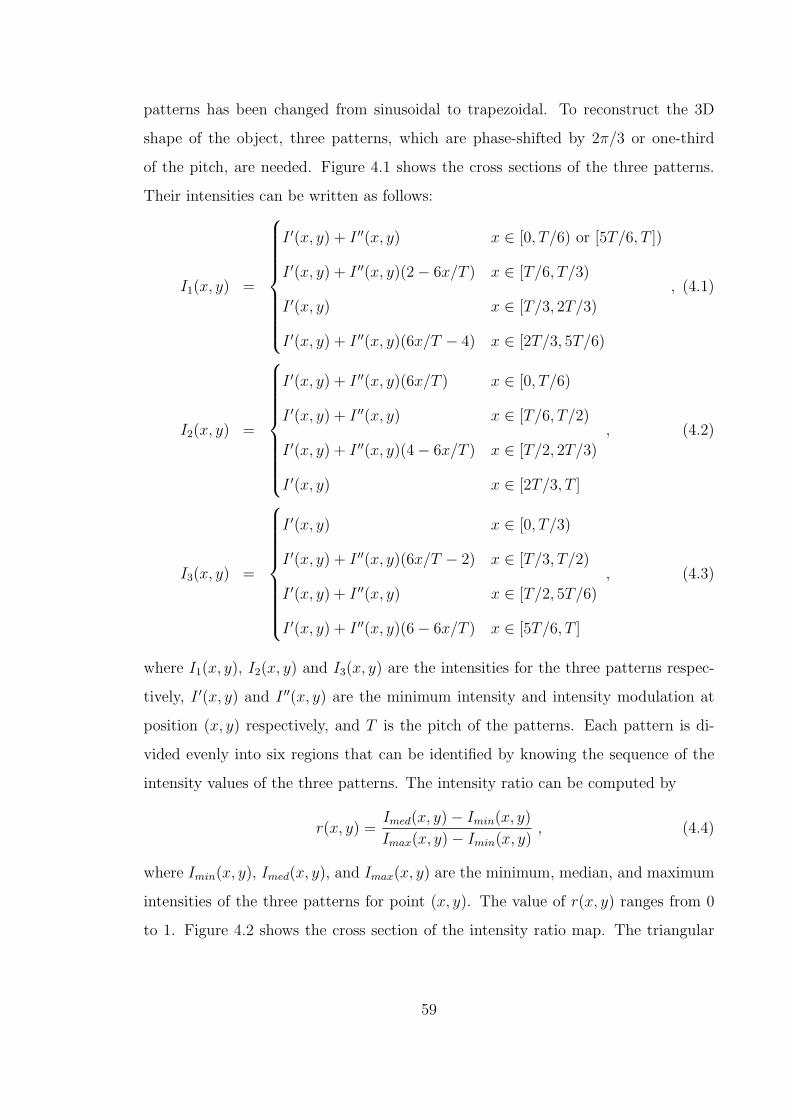
patterns has been changed from sinusoidal to trapezoidal. To reconstruct the 3D

shape of the object, three patterns, which are phase-shifted by 2π/3 or one-third

of the pitch, are needed. Figure 4.1 shows the cross sections of the three patterns.

Their intensities can be written as follows:

I1(x, y) =

I ′(x, y) + I ′′(x, y) x ∈ [0, T/6) or [5T/6, T ])

I ′(x, y) + I ′′(x, y)(2− 6x/T ) x ∈ [T/6, T/3)

I ′(x, y) x ∈ [T/3, 2T/3)

I ′(x, y) + I ′′(x, y)(6x/T − 4) x ∈ [2T/3, 5T/6)

, (4.1)

I2(x, y) =

I ′(x, y) + I ′′(x, y)(6x/T ) x ∈ [0, T/6)

I ′(x, y) + I ′′(x, y) x ∈ [T/6, T/2)

I ′(x, y) + I ′′(x, y)(4− 6x/T ) x ∈ [T/2, 2T/3)

I ′(x, y) x ∈ [2T/3, T ]

, (4.2)

I3(x, y) =

I ′(x, y) x ∈ [0, T/3)

I ′(x, y) + I ′′(x, y)(6x/T − 2) x ∈ [T/3, T/2)

I ′(x, y) + I ′′(x, y) x ∈ [T/2, 5T/6)

I ′(x, y) + I ′′(x, y)(6− 6x/T ) x ∈ [5T/6, T ]

, (4.3)

where I1(x, y), I2(x, y) and I3(x, y) are the intensities for the three patterns respec-

tively, I ′(x, y) and I ′′(x, y) are the minimum intensity and intensity modulation at

position (x, y) respectively, and T is the pitch of the patterns. Each pattern is di-

vided evenly into six regions that can be identified by knowing the sequence of the

intensity values of the three patterns. The intensity ratio can be computed by

r(x, y) =Imed(x, y)− Imin(x, y)

Imax(x, y)− Imin(x, y), (4.4)

where Imin(x, y), Imed(x, y), and Imax(x, y) are the minimum, median, and maximum

intensities of the three patterns for point (x, y). The value of r(x, y) ranges from 0

to 1. Figure 4.2 shows the cross section of the intensity ratio map. The triangular

59

shape can be removed to obtain a ramp by using the following equation:

r(x, y) = 2× round

(N − 1

2

)+ (−1)N+1 Imed(x, y)− Imin(x, y)

Imax(x, y)− Imin(x, y), (4.5)

where Imin(x, y), Imed(x, y), and Imax(x, y) are the minimum, median, and maximum

intensities of the three patterns for point (x, y). The value of r(x, y) ranges from 0

to 1. Figure 4.2 shows the cross section of the intensity ratio map. The triangular

shape can be removed to obtain a ramp by using the following equation:

r(x, y) = 2× round

(N − 1

2

)+ (−1)N+1 Imed(x, y)− Imin(x, y)

Imax(x, y)− Imin(x, y), (4.6)

where N = 1, 2, ...6 is the region number, which is determined by comparing the

three intensity values at each point. After the removal of the triangular shape, the

value of r(x, y) now ranges from 0 to 6, as shown in Figure 4.3. If multiple fringes are

used, the intensity ratio is wrapped into this range of 0 to 6 and has a sawtooth-like

shape. A process similar to phase unwrapping in the traditional sinusoidal phase-

shifting method needs to be used. The Depth information can be obtained from

this intensity ratio based on an algorithm similar to the phase-to-height conversion

algorithm used in the sinusoidal phase-shifting method.(see Section 3.2.5).

4.3 Error Analysis

In this research, a DLP video projector was used to project the trapezoidal

fringe patterns to the object. The images are captured by a CCD camera. The ma-

jor potential error sources are the image defocus error due to limited depth of focus

of both the projector and the camera and the nonlinear gamma curve of the projec-

tor. The nonlinear gamma curve can be corrected by software. (see Section 3.2.4).

However, the residual nonlinearity can still cause errors that cannot be ignored. The

following sections discuss the effects of these two error sources.

4.3.1 Image defocus error

In the sinusoidal phase-shifting method, image defocus will not cause major

errors because a sinusoidal pattern will still be a sinusoidal pattern when the image

60

x

I'(x, y)

I"(x, y)

I1(x,y) N = 1 2 3 4 5 6

T/6 T/3 T/2 2T/3 5T/6

(a) Cross section of I1

x

I'(x, y)

I"(x, y)

I2(x,y) N = 1 2 3 4 5 6

T/6 T/3 T/2 2T/3 5T/6 T

(b) Cross section of I2

x

I"(x, y)

I3(x,y) N = 1 2 3 4 5 6

T/6 T/3 T/2 2T/3 5T/6

I0(x, y)

(c) Cross section of I3

Figure 4.1: Phase-shifted trapezoidal fringe patterns.

x0

1

T/6 T/3 T/2 2T/3 5T/6 T0

N = 1 2 3 4 5 6r(x, y)

Figure 4.2: Cross section of the intensity-ratio map.

123456

x

r(x, y)

T/6 T/3 T/2 2T/3 5T/6 T0

N = 1 2 3 4 5 6

Figure 4.3: Cross section of the intensity-ratio map after removal of the triangles.

is defocused, even though the fringe contrast may be reduced. However, in the

trapezoidal phase-shifting method, image defocus will blur the trapezoidal pattern,

which may cause errors that cannot be ignored. In order to quantify this error, we

use a Gaussian filter to simulate the defocusing effect. By changing the size of the

filter window, we can simulate the level of defocus and calculate the corresponding

error. Following is the equation for the intensity ratio r(x, y) when the fringe images

61

are defocused:

r(x, y) =Imed(x, y)⊗G(x, y)− Imin(x, y)⊗G(x, y)

Imax(x, y)⊗G(x, y)− Imin(x, y)⊗G(x, y), (4.7)

where symbol ⊗ denotes the convolution operation and

G(x, y) =1

2πσ2e−(x−x)2−(y−y)2

2σ2 ,

is a 2D Gaussian filter, which is a 2D normal distribution with standard deviation σ

and mean point coordinate (x, y).

To simplify the analysis without loosing its generality, we consider only a 1-D

case (along x-axis) within regions N = 1 and N = 2. Assuming the size of the filter

window to be (2M + 1) pixels, we obtain the discrete form of the intensity ratio

function as

rdef (x, y) =

∑T/6−x−1n=−M [6(x+n)/T ]G(n)+

∑Mn=T/6−x G(n)

∑T/6−x−1n=−M G(n)+

∑Mn=T/6−x G(n)[2−6(x+n)/T ]

x ∈ [0, T/6)

∑T/6−x−1n=−M G(n)+

∑Mn=T/6−x G(n)[2−6(x+n)/T ]

∑T/6−x−1n=−M [6(x+n)/T ]G(n)+

∑Mn=T/6−x G(n)

x ∈ [T/6, T/3)

, (4.8)

where

G(n) =

e−n2

2σ2 /∑M

n=−M e−n2

2σ2 n ∈ [−M, M ]

0 otherwise

,

is a 1-D discrete Gaussian filter with standard deviation σ. To show the effect of

image defocus on intensity ratio, we calculate rdef (x) for a filter window size of T and

compare it with r(x), which is the intensity ratio without image defocus. The results

are shown in Figure 4.4. We can see that image defocus causes the originally linear

intensity ratio to become nonlinear, which introduces distortion to the measured

shape. To quantify the effect of image defocus on intensity ratio as a function of the

level of defocus, we define error E as follows:

E = {max[rdef (x)− r(x)]−min[rdef (x)− r(x)]}/6 . (4.9)

Figure 4.5 shows how this error value changes as the size of the filter window increases

from 0 to T . From this figure, we see that the error increases with the window size

up until the window size reaches about 0.7T . After that, the error is stabilized

62

0 0.2 0.4 0.6 0.8 10

0.2

0.4

0.6

0.8

1

0

0.2

0.4

0.6

0.8

x ( x T/6)

Inte

nsity

rat

io

With defocusWithout defocus

Figure 4.4: Comparison of the intensity ratios with and without image defocus. Herethe filter window size used in the calculation is T .

0 0.2 0.4 0.6 0.8 10

0.2

0.4

0.6

0.8

Filter window size ( x T )

Err

or (

%)

Figure 4.5: Maximum error due to image defocus.

to a relatively small value of 0.6%. This phenomenon is due to the fact that as

the window size, or the defocus level, is increased, the trapezoidal pattern becomes

increasingly like a sinusoidal pattern and once becoming a sinusoidal pattern, the

error does not change anymore even if it is further defocused. Figure 4.6 shows

how the trapezoidal pattern is blurred for different window sizes. Clearly, when the

window size is increased to T , the pattern is already like a sinusoidal pattern. This

error depends on the window size of the filter or the level of defocus.

To understand why for such dramatic defocusing of the fringe pattern the error

is still limited to only about 0.6%, we can look at the transitional area between

regions N = 1 and N = 2, which is shown in Figure 4.7. We can see that the

63

Figure 4.6: Blurring effect of the trapezoidal fringe pattern due to image defocus.

(x, I(x))

I1(x)

Filter window

I2(x)I

2-ideal

I1-defocus

Filter size (2M + 1)

I1-ideal

I2-defocus

N = 1 N = 2

Figure 4.7: Enlarged view of the blurring effect of the trapezoidal fringe pattern inthe borderline area between regions N = 1 and N = 2.

cross sections of I1(x, y) and I2(x, y) are symmetrical with respect to the borderline

of the two regions. Even when the fringe patterns are defocused, this symmetry is

maintained. This results in similar drops in I1(x, y) and I2(x, y) in the regions close to

the borderline, which reduces the error in the calculation of the ratio I1(x, y)/I2(x, y).

At the borderline of the two regions, the ratio, which still equals to one, does not

change even after the images are defocused.

In summary, even though the trapezoidal phase-shifting method is still sensitive

to the defocusing effect (unlike the sinusoidal phase-shifting method), the resulting

error is small, in particular when compared to conventional intensity ratio based

methods. For example, for a filter window size of 0.1T , the method proposed by

Savarese et al. will have an error of more than 53% [34], while the error of the trape-

zoidal phase-shifting method will only be approximately 0.03%, which is dramatically

smaller. Therefore, the trapezoidal phase-shifting method is capable of measuring

objects with large depth with limited errors.

64

4.3.2 Nonlinearity error

The relationship between the input grayscale values and the grayscale cap-

tured by the camera should be linear. Otherwise it will result in errors in the final

measurement results. Since the gamma curve of the projector is usually not linear,

we use a software compensation method to linearize this relationship. However, the

relationship after compensation may still not be exactly linear. This nonlinearity

directly affects the measurement accuracy. In fact, the shape of the ratio curve in

each region, which should be linear ideally, is a direct replica of the gamma curve, if

no defocusing effect is considered. Therefore, reducing the nonlinearity of the gamma

curve is critical to the measurement accuracy.

4.4 Experiments

To verify its performance, we implemented the trapezoidal phase-shifting method

in our real-time 3D shape measurement system. To increase the image resolution,

we used periodic patterns with a pitch of 12 pixels per fringe. The 3D result was ob-

tained after removing the periodical discontinuity by adding or subtracting multiples

of 6, which is similar to phase unwrapping in the sinusoidal phase-shifting method.

Figure 4.8 shows the measured shape of a cylindrical part with a diameter of

200 mm. Figure 4.8(a) shows the cross section of the measured patch as compared

to the ideal curve, Figure 4.8(b) shows the difference or error, and Figure 4.8(c)

shows the 3D plot. As can be seen from the result, the measurement is accurate

(the peak-to-peak error is approximately 0.6 mm) for most part of the surface except

for the left 20 mm or so, which shows a significant error. This large error is due

to the slope of the surface in that area, which makes the surface almost parallel to

the projection light. Figure 4.9 shows the measured result of a plaster sculpture

head. The measurement resolution is comparable to that of the sinusoidal phase-

shifting method. The advantage lies in the processing speed of the fringe patterns,

thanks to the simple intensity-ratio calculation as opposed to the phase calculation

with an arctangent function in the sinusoidal phase-shifting method. This enables

potential real-time 3D shape measurement for objects with dynamically changing

65

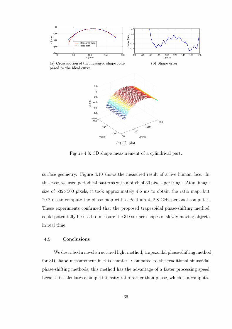
0 50 100 150 200−80

−60

−40

−20

0

x (mm)

z (m

m)

Measured dataIdeal data

(a) Cross section of the measured shape com-pared to the ideal curve.

20 40 60 80 100 120 140 160 180

−0.4

−0.2

0

0.2

0.4

x (mm)

z er

ror

(mm

)

(b) Shape error

50

100

150

200

100

150

200−100

−80

−60

−40

−20

0

20

x(mm)y(mm)

z(m

m)

(c) 3D plot

Figure 4.8: 3D shape measurement of a cylindrical part.

surface geometry. Figure 4.10 shows the measured result of a live human face. In

this case, we used periodical patterns with a pitch of 30 pixels per fringe. At an image

size of 532×500 pixels, it took approximately 4.6 ms to obtain the ratio map, but

20.8 ms to compute the phase map with a Pentium 4, 2.8 GHz personal computer.

These experiments confirmed that the proposed trapezoidal phase-shifting method

could potentially be used to measure the 3D surface shapes of slowly moving objects

in real time.

4.5 Conclusions

We described a novel structured light method, trapezoidal phase-shifting method,

for 3D shape measurement in this chapter. Compared to the traditional sinusoidal

phase-shifting methods, this method has the advantage of a faster processing speed

because it calculates a simple intensity ratio rather than phase, which is a computa-

66

(a) I1 (b) I2 (c) I3 (d) 3D wireframe (e) 3D shaded

Figure 4.9: 3D shape measurement of a plaster sculpture.

Figure 4.10: 3D shape measurement of human faces.

tionally more time-consuming arctangent function. The depth resolution is similar.

The disadvantage is that image defocus may cause some errors, even though they are

quite small. Compared to the traditional intensity-ratio based methods, this method

has a depth resolution that is six times better. It is also significantly less sensitive to

image defocus, which allows it to be used to measure objects with large depth vari-

ations. Experimental results demonstrated that the newly proposed method could

be used to provide 3D surface shape measurements for both static and dynamically

changing objects. However, for measurement requiring high accuracy, the small error

caused by image defocusing is non-negligible.

67

Chapter 5

Fast Phase-wrapping Algorithm

Trapezoidal phase-shifting algorithm has the advantages of high processing

speed, but its accuracy is affected by image defocusing. From analysis in Chapter 4,

we know that the maximum error caused by image defocusing is 0.6%, which occurs

when the trapezoidal pattern becomes sinusoidal pattern due to excessive defocus. In

this chapter, we propose a new three-step algorithm which replaces the calculation

of the arctangent function with a simple ratio calculation and therefore is much

faster than the traditional algorithm. The phase error caused by this replacement

is compensated for by use of a look-up-table (LUT). Our experimental results show

that the error caused by this fast processing algorithm is negligible. The adoption of

this new algorithm enabled us to successfully build a high-resolution, real-time 3D

shape measurement system that captures, reconstructs, and displays the 3D shape

of measured objects in real time at a speed of 40 frames per second and a resolution

of 532× 500 pixels, all with an ordinary personal computer.

5.1 Introduction

Sinusoidal three-step phase-shifting algorithm has the merit of fast and accu-

rate 3D shape measurement, and is feasible for real-time 3D measurement. However,

our experiments show that even with the three-step algorithm, the image processing

speed is not fast enough for real-time 3D shape reconstruction. The bottleneck lies

in the calculation of phase, which involves a computationally time-consuming arct-

angent function. To solve this problem, we propose a fast phase-wrapping algorithm,

68

which replaces the calculation of the arctangent function with a simple ratio calcu-

lation and therefore is much faster than the traditional algorithm. The phase error

caused by this replacement is compensated for by use of a look-up-table (LUT). Our

simulation and experimental results show that both the new algorithm and the tradi-

tional algorithm generate similar results, but the new algorithm is at least 3.4 times

faster.The adoption of this new algorithm enables us to successfully build a high-

resolution, real-time 3D shape measurement system that captures, reconstructs, and

displays the 3D shape of the measured object in real time at a speed of 40 frames per

second and a resolution of 532× 500 pixels, all with an ordinary personal computer.

Section 5.2 explains the principle of the fast phase-wrapping algorithm. Sec-

tion 5.3 analyzes the processing error and proposes an error reduction method. Sec-

tion 5.4 shows some experimental results. And Section 5.5 concludes the chapter.

5.2 Principle

The traditional three-step phase-shifting algorithm works well in terms of accu-

racy [73]. However, due to the need of computing an arctangent function for phase,

the reconstruction of 3D shape is relatively time consuming. This section addresses

the principle of the proposed fast phase-wrapping algorithm based on the trapezoidal

phase-shifting algorithm discussed in Chapter 4.

5.2.1 Fourier analysis of the trapezoidal phase-shifting algorithm

Sinusoidal fringe patterns can be viewed as severely defocused trapezoidal fringe

patterns. From discussion in Chapter 4, we know that the error caused by image

defocus peaks at approximately 0.6%, which is rather small. This means that even

if we use the algorithm developed for the trapezoidal fringe patterns to process sinu-

soidal fringe patterns, the error should be limited. Here we use Fourier analysis to

show this indeed the case.

From the plots shown in Figure 4.1, we know that the trapezoidal fringe pat-

69

terns are each shifted by 1/3 period, T . That is

I2(x, y) = I1

(x− T

3, y

), (5.1)

I3(x, y) = I2

(x− T

3, y

). (5.2)

Since the shape of the first pattern is symmetric to y axis, its Fourier expansion is a

cosine series along x-axis,

I1(x, y) =a0

2+

∞∑m=1

am cos

(2πm

Tx

), (5.3)

where

a0 =2

T

∫ T

0

I1(x, y)dx = 1 , (5.4)

am =2

T

∫ T

0

I1(x, y) cos

(2πm

Tx

)dx

=12

(mπ)2sin

(mπ

2

)sin

(mπ

6

). (5.5)

Therefore,

I1(x, y) =1

2+

∞∑m=1

12

(mπ)2sin

(mπ

2

)sin

(mπ

6

)cos

(2πm

Tx

). (5.6)

From Equations 5.1, 5.2 and 5.6, we obtain

I2(x, y) =1

2+

∞∑m=1

12

(mπ)2sin

(mπ

2

)sin

(mπ

6

)cos

[2πm

T

(x− T

3

)]. (5.7)

I3(x, y) =1

2+

∞∑m=1

12

(mπ)2sin

(mπ

2

)sin

(mπ

6

)cos

[2πm

T

(x− 2T

3

)]. (5.8)

For region N = 1, x ∈ [0, T/6), the intensity ratio in Equation 4.4 can be obtained

as,

r(x, y) =

∑∞m=1

1m2 sin

(mπ2

)cos

(mπ6

)sin

[2mπ

T

(x− T

2

)]∑∞

m=11

m2 sin(

mπ2

)cos

(mπ6

)sin

[2mπ

T

(x− T

3

)] . (5.9)

By observing Equation 5.9, we see that the r(x, y) is determined by 1×, 5×, 7×, · · · ,frequency components only. Since comparing to the 1× frequency component, the

5×, and 7× frequency components are 1/25 and 1/49 smaller respectively, r(x, y)

can be approximated by including only the 1× frequency component without causing

70

I'(x, y)

N = 1 2 3 4 5 6

I"(x, y)

I1(x, y)

(x, y)T/6 T/3 T/2 2T/3 5T/6 T

(a) I1(−2π/3)

I'(x, y)

N = 1 2 3 4 5 6

I"(x, y)

I2(x, y)

(x, y)T/6 T/3 T/2 2T/3 5T/6 T

(b) I2(0)

I'(x, y)

I3(x,y) N = 1 2 3 4 5 6

I"(x, y)

(x, y)T/6 T/3 T/2 2T/3 5T/6 T

(c) I3(2π/3)

Figure 5.1: Cross sections of the three phase-shifted sinusoidal patterns.

significant errors. However, when only the 1× frequency component is included, the

trapezoidal fringe pattern effectively becomes a sinusoidal fringe pattern. Therefore,

we can conclude that using the algorithm developed for the trapezoidal phase-shifting

method to process sinusoidal fringe patterns will not result in significant error.

5.2.2 Fast phase-wrapping algorithm

Similar to trapezoidal phase-shifting algorithm, the sinusoidal fringe images can

be evenly divided into 6 regions in one period (T = 2π). Figure 5.1 shows the cross

sections of the sinusoidal fringe patterns. We use the same equation (Equation 4.4)

developed for the trapezoidal phase-shifting method to calculate the intensity ratio.

That is

r(x, y) =Imed(x, y)− Imin(x, y)

Imax(x, y)− Imin(x, y). (5.10)

where Imin(x, y), Imed(x, y) and Imax(x, y) are the minimum, median, and maximum

intensities of the three patterns for point (x, y). The value of r(x, y) ranges from 0

to 1. Figure 5.2 shows the cross section of the intensity ratio map. Similarly, the

71

0

N = 1 2 3 4 5 6

T/6 T/3 T/2 2T/3 5T/6 T

r(x, y)

(x, y)

1

Figure 5.2: Cross section of the intensity ratio map.

0

N = 1 2 3 4 5 6

T/6 T/3 T/2 2T/3 5T/6 T (x, y)

(x, y)2

Figure 5.3: Cross section of the intensity ratio map after removal of the triangularshape.

triangular shape can be removed to obtain wrapped intensity ratio map by using

Equation 4.5. The phase can then be calculated by the following equation,

φ(x, y) =π

3

[2× round

(N

2

)+ (−1)Nr(x, y)

], (5.11)

whose value ranges from 0 to 2π, as shown in Figure 5.3. As we can see from the figure

that the phase calculation is not accurate, but with a small error. In Section 5.3, we

will analyze this error and discuss how this error can be compensated for.

If multiple fringes are used, the phase calculated by Equation 5.11 will result in

a sawtooth-like shape, just as in the traditional phase shifting algorithm. Therefore,

the traditional phase-unwrapping algorithm can be used to obtain the continuous

phase map.

5.3 Error Analysis and Compensation

Fast phase-wrapping algorithm has the advantage of fast processing speed over

traditional phase shifting algorithm. However, this method makes the linear phase

value φ(x, y) to be nonlinear, as shown in Figure 5.3, which produces error. In this

section, we discuss the error caused by applying fast phase-wrapping algorithm for

sinusoidal patterns first and then propose an error compensation method.

72

From Figure 5.3, we see that the error is periodical and the pitch is π/3.

Therefore, we only need to analyze the error in one period, say φ(x, y) ∈ [0, π/3).

In this period, Ih(x, y) = I2(x, y), Im(x, y) = I1(x, y), and Il(x, y) = I3(x, y). By

substituting Equations 2.11 into Equation 5.10, we obtain

r(φ) =I1 − I3

I2 − I3

=1

2+

√3

2tan

(φ− π

6

). (5.12)

The right-hand side of this equation can be considered as the sum of a linear and a

nonlinear terms. That is

r(φ) =φ

π/3+ ∆r(φ) , (5.13)

where the first term represents the linear relationship between r(x, y) and φ(x, y)

and the second term ∆r(x, y) is the nonlinearity error, which can be calculated as

follows:

∆r(φ) = r(φ)− φ

π/3

=1

2+

√3

2tan

(φ− π

6

)− φ

π/3. (5.14)

Figure 5.4(a) shows the plots of both the ideal linear ratio and the real nonlinear ratio.

Their difference, which is similar to a sine wave in shape, is shown in Figure 5.4(b).

By taking the derivative of ∆r(x, y) with respect to φ(x, y) and setting it to zero, we

can determine that when

φ(φ) =π

6± arccos

(√√3π/6

), (5.15)

the ratio error reaches its maximum and minimum values respectively as

∆r(φ)max = ∆r(φ)|φ=φ1 = 0.0186 , (5.16)

∆r(φ)min = ∆r(φ)|φ=φ2 = −0.0186 . (5.17)

Therefore, the maximum ratio error is ∆r(φ)max − ∆r(φ)min = 0.0372. Since the

maximum ratio value for the whole period is 6, the maximum ratio error in terms of

percentage is 0.0372/6 = 0.6%. Even though this error is relatively small, it needs

to be compensated for when accurate measurement is required.

73

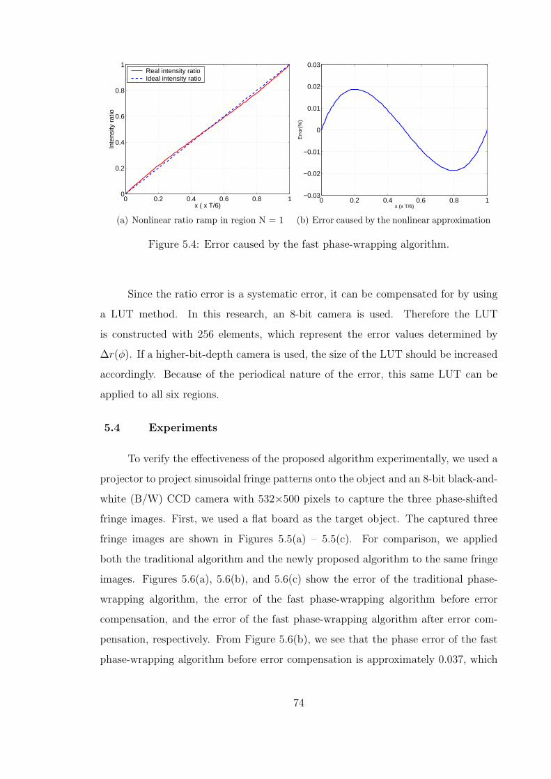
0 0.2 0.4 0.6 0.8 10

0.2

0.4

0.6

0.8

1

x ( x T/6)

Inte

nsity

rat

io

Real intensity ratioIdeal intensity ratio

(a) Nonlinear ratio ramp in region N = 1

0 0.2 0.4 0.6 0.8 1−0.03

−0.02

−0.01

0

0.01

0.02

0.03

x (x T/6)

Err

or(%

)

(b) Error caused by the nonlinear approximation

Figure 5.4: Error caused by the fast phase-wrapping algorithm.

Since the ratio error is a systematic error, it can be compensated for by using

a LUT method. In this research, an 8-bit camera is used. Therefore the LUT

is constructed with 256 elements, which represent the error values determined by

∆r(φ). If a higher-bit-depth camera is used, the size of the LUT should be increased

accordingly. Because of the periodical nature of the error, this same LUT can be

applied to all six regions.

5.4 Experiments

To verify the effectiveness of the proposed algorithm experimentally, we used a

projector to project sinusoidal fringe patterns onto the object and an 8-bit black-and-

white (B/W) CCD camera with 532×500 pixels to capture the three phase-shifted

fringe images. First, we used a flat board as the target object. The captured three

fringe images are shown in Figures 5.5(a) – 5.5(c). For comparison, we applied

both the traditional algorithm and the newly proposed algorithm to the same fringe

images. Figures 5.6(a), 5.6(b), and 5.6(c) show the error of the traditional phase-

wrapping algorithm, the error of the fast phase-wrapping algorithm before error

compensation, and the error of the fast phase-wrapping algorithm after error com-

pensation, respectively. From Figure 5.6(b), we see that the phase error of the fast

phase-wrapping algorithm before error compensation is approximately 0.037, which

74

(a) I1(−2π/3) (b) I2(0◦) (c) I3(2π/3)

Figure 5.5: Fringe images of a flat board captured by a 8-bit B/W CCD camera.

agrees well with the theoretical analysis. After error compensation, this error, which

is shown in Figure 5.6(c), is significantly reduced and is comparable to that of the

traditional phase-wrapping algorithm as shown in Figure 5.6(a).

Next, we measured an triangular shape object with multiple fringe images. The

captured fringe images are shown in Figures 5.7(a)– 5.7(c). The reconstructed 3D

shapes using the traditional algorithm and the proposed algorithm to these fringe

images are shown in Figures 5.7(d) and 5.7(e), respectively. The difference between

these reconstructed result is shown in Figure 5.7(f), which is approximately ±0.002

mm and is negligible.

Finally, we measured an object with more complex surface geometry, a Lin-

coln head sculpture. The 2-D photo of the object is shown in Figure 5.8(a). The

reconstructed 3-D shapes based on the traditional and the proposed phase-wrapping

algorithms are shown in Figures 5.8(b) and 5.8(c), respectively. We can see that the

two results show almost no difference.

In our experiment, we used an ordinary personal computer (Pentium 4, 2.8GHz)

for image processing. The traditional phase-wrapping algorithm took 20.8 ms, while

the proposed new algorithm took only 6.1 ms, which was 3.4 times less. The im-

provement in processing speed is significant.

75

0 100 200 300 400 500−0.03

−0.02

−0.01

0

0.01

0.02

0.03

pixel

Err

or

(a)

0 100 200 300 400 500−0.03

−0.02

−0.01

0

0.01

0.02

0.03

pixel

Err

or

(b)

0 100 200 300 400 500−0.03

−0.02

−0.01

0

0.01

0.02

0.03

pixel

Err

or

(c)

Figure 5.6: Residual phase error. (a) With the traditional algorithm. (b) With theproposed algorithm before error compensation. (c) With the proposed algorithmafter error compensation.

5.5 Conclusion

In this chapter, we proposed a fast phase-wrapping algorithm based on intensity

ratio calculation and LUT error compensation for real-time 3-D shape measurement.

This algorithm originated from the previously proposed trapezoidal phase shifting

method, which was aimed at improving the processing speed of the fringe images.

In this research, we found that the same algorithm developed for the trapezoidal

fringe patterns could be used to process sinusoidal fringe images with a small error,

which could be easily eliminated by using a LUT method. This finding resulted in

a new phase-wrapping algorithm that is 3.4 times faster than and just as accurate

as the traditional phase-wrapping algorithm. Experimental results demonstrated

the effectiveness of the proposed algorithm. We have successfully implemented this

algorithm in our real-time 3-D shape measurement system, which has a frame rate

of 40 frames per second and a resolution of 532 × 500 points.

76

(a) (b) (c)

(d) (e) 3D by fast wrapping

0 50 100 150 200−0.04

−0.02

0

0.02

0.04

x (mm)

z (m

m)

(f) 250th row of 3D difference

Figure 5.7: Reconstructed 3D result of a sheet metal by fast phase-wrapping algo-rithm. (a) I0(−2π/3. (b) I1(0). (c) I2(2π/3). (d) 3D shape using the traditionalphase-wrapping algorithm. (e) 3D shape using the fast phase-wrapping algorithm.(f) 3D shape difference using the traditional and the fast phase-wrapping algorithms.

(a) (b) (c)

Figure 5.8: 3D reconstruction results of sculpture Lincoln. (a)2D photo. (b)3Dshape using the traditional phase-wrapping algorithm. (c)3D shape using the fastphase-wrapping algorithm.

77

Chapter 6

Error Compensation Algorithm

This chapter addresses a novel error compensation technique for reducing the

measurement error caused by nonsiusoidal waveforms in the phase-shifting method.

For 3D measurement systems using commercial video projectors, the non-sinusoidal

nature of the projected fringe patterns as a result of the nonlinear projection response

curve (or gamma curve) of the projectors causes significant phase measurement error

and therefore shape measurement error. The proposed error compensation method

is based on our finding that the phase error due to non-sinusoidal fringe patterns

depends only on the nonlinearity of the projector’s gamma curve. Therefore, if the

projector’s gamma curve is calibrated and the phase error due to the nonlinearity

of the gamma curve is calculated, a look-up-table (LUT) that stores the phase error

can be constructed for error compensation. Our experimental results demonstrate

that by using the proposed method, the measurement error can be reduced by 10

times. In addition to phase error compensation, a similar method is also proposed

to correct the non-sinusoidality of the fringe patterns for the purpose of generating

a more accurate flat image of the object for texture mapping, which is important for

applications in computer vision and computer graphics.

6.1 Introduction

With the development of digital display technologies, commercial digital video

projector are more and more broadly used in 3D measurement systems. The error due

to non-sinusoidal waveforms is one of the major errors of 3D measurement systems

78

based on the phase shifting method. The non-sinusoidal nature of the projected

fringe patterns as a result of the nonlinear gamma curve of the projectors causes

significant phase measurement error and therefore shape measurement error. Pre-

viously proposed methods, such as, double three-step phase-shifting algorithm [74],

3+3 phase-shifting algorithm [73], direct correction of the nonlinearity of the pro-

jector’s gamma curve [65], demonstrated significant reduction of the measurement

error, but the residual error remains non-negligible. In this research, we propose a

novel error compensation method that can produce significantly better results. This

method is developed based on our finding that the phase error due to non-sinusoidal

fringe patterns depends only on the nonlinearity of the projector’s gamma curve.

Therefore, if the projector’s gamma curve is calibrated and the phase error due to

the nonlinearity of the gamma curve is calculated, a look-up-table (LUT) that stores

the phase error can be constructed for error compensation. In addition to error

compensation, a similar method is also proposed to correct the non-sinusoidality of

the fringe patterns for the purpose of generating a more accurate flat image of the

object for texture mapping, which is important for applications in computer vision

and computer graphics.

In this chapter, Section 6.2 introduces the theoretical background of the this

error compensation method, Section 6.3 shows simulation results, Section 6.4 shows

experimental results, Section 6.5 discusses the advantages and limitations of the

method, and Section 6.6 concludes the chapter.

6.2 Principle

6.2.1 Phase correction

The images captured by the camera is formed through the procedure illustrated

in Figure 6.1. Without loss of generality, we consider only the three-step phase-

shifting algorithm with a phase shift of 2π/3 (see Section 2.2.3). Let us assume

that the projector’s input sinusoidal fringe images generated by a computer have the

79

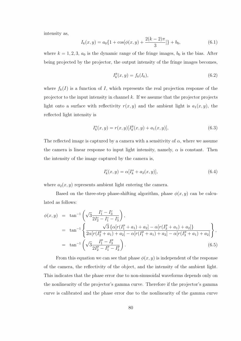
intensity as,

Ik(x, y) = a0{1 + cos[φ(x, y) +2(k − 2)π

3]}+ b0, (6.1)

where k = 1, 2, 3, a0 is the dynamic range of the fringe images, b0 is the bias. After

being projected by the projector, the output intensity of the fringe images becomes,

Ipk(x, y) = fk(Ik), (6.2)

where fk(I) is a function of I, which represents the real projection response of the

projector to the input intensity in channel k. If we assume that the projector projects

light onto a surface with reflectivity r(x, y) and the ambient light is a1(x, y), the

reflected light intensity is

Iok(x, y) = r(x, y)[Ip

k(x, y) + a1(x, y)], (6.3)

The reflected image is captured by a camera with a sensitivity of α, where we assume

the camera is linear response to input light intensity, namely, α is constant. Then

the intensity of the image captured by the camera is,

Ick(x, y) = α[Io

k + a2(x, y)], (6.4)

where a2(x, y) represents ambient light entering the camera.

Based on the three-step phase-shifting algorithm, phase φ(x, y) can be calcu-

lated as follows:

φ(x, y) = tan−1

(√3

Ic1 − Ic

3

2Ic2 − Ic

1 − Ic3

),

= tan−1

{ √3 {α[r(Ip

1 + a1) + a2]− α[r(Ip3 + a1) + a2]}

2α[r(Ip2 + a1) + a2]− α[r(Ip

1 + a1) + a2]− α[r(Ip3 + a1) + a2]

},

= tan−1

(√3

Ip1 − Ip

3

2Ip2 − Ip

1 − Ip3

). (6.5)

From this equation we can see that phase φ(x, y) is independent of the response

of the camera, the reflectivity of the object, and the intensity of the ambient light.

This indicates that the phase error due to non-sinusoidal waveforms depends only on

the nonlinearity of the projector’s gamma curve. Therefore if the projector’s gamma

curve is calibrated and the phase error due to the nonlinearity of the gamma curve

80

k I p

k I o

k I c

k I

Object Projector Camera Object Projector Camera

Figure 6.1: Camera image generation procedure.

is calculated, a look-up-table (LUT) that stores the phase error can be constructed

for error compensation.

The following steps describe the procedure of constructing the LUT:

(1) Sample projection response functions. A series of gray scale images with

different grayscale values In, n = 1, 2, · · · , N , are sent to the projector. The

projector projects the gray scale images with intensity values fk(In) onto

a white board. The reflected images are captured by the camera and the

intensities at the center of the images, Ickn, are calculated. The set of samples

(In, Ickn) is recorded.

(2) Approximate the projection response functions fk. The projection response

functions fk(In) are constructed through fitting the sample points by spline

curves. Figure 6.2 illustrates a typical example of our reconstructed projec-

tion response curves for R, G, B channels. It is obvious that the curves are

non-linear and unbalanced.

(3) Find a straight line f(I), such that f(I1) = max{fk(I1)}, f(IN) = min{fk(IN)},f is considered the ideal projection response for all channels.

(4) Compute real phase φ using Equation 6.5.

(5) Compute the ideal phase φ by replacing fk in Equation 6.5 with f .

(6) Record the difference φ− φ and store (φ, φ− φ) in a phase error LUT.

The constructed phase error LUT can be used to correct phase error for real

measurements. It only depends on the projection response functions fk and can be

81

0 50 100 150 200 2500

20

40

60

80

100

120

140

160

180

200

Input grayscale values to the projector

Out

put g

rays

cale

val

ues

capt

ured

by

cam

era

(115)(58) (224)

RGBIdeal

Figure 6.2: Typical projection response curve.

constructed once for all as long as the fk’s are unchanged. The same method can

be applied to correct nonsinusoidal fringe images, which is very important for many

applications that require high quality texture.

6.2.2 Texture recovering

Ideally, the texture of image can be generated by averaging the three phase-

shifted fringe images with 2π/3 of phase shift. However, if the fringe images are

not exactly sinusoidal, the texture image can not be correctly obtained by simple

averaging. We found that the fringe images could be recovered by a solving reverse

problem.

It is obvious that (φ, fk) forms a one-to-one map in one period φ ∈ [0, 2π), and

fk is monotonous and invertible. Therefore, for a given phase value φ ranging from

0 to 2π, the corresponding points (Ik, fk(Ik)) can be uniquely determined. Further-

more, its corresponding point (Ik, f(Ik)) on the ideal projection response curve can

also be determined. Hence, ratio Rk := fk/f for any given φ is well defined. We can

build a ratio map (φ, Rk) to correct the nonsinusoidal fringe images and to produce

correct texture images by averaging the correct sinusoidal fringe images.

The following describes the procedure. Again, assume the camera is linear with

82

constant response α. Without loss of generality, we assume

f(I1) = max{fk(I1)} = f3(I1),

f(IN) = min{fk(IN)} = f1(IN),

Then the ideal projection response function is

f(I) =f1(IN)− f3(I1)

IN − I1

(I − I1) + f3(I1).

Based on the virtual ideal linear projection response function, the camera image

intensity is

Icideal(x, y) = α[r(x, y)(f(I) + a1(x, y)) + a2(x, y)],

Then ratio,

Rk(x, y) =Ick

Icideal

=α[r(fk + a1) + a2]

α[r(f + a1) + a2]=

r(fk + a1) + a2

r(f + a1) + a2

, (6.6)

If a1(x, y) and a2(x, y) are very small (near zero), then this equation can be approx-

imated as

Rk(x, y) ≈ fk

f. (6.7)

From this equation we can see that ratio Rk(x, y) is independent of the response of

the camera, the reflectivity of the object, and the intensity of the ambient light. This

means that the ratio map depends only on the nonlinearity of the projector’s gamma

curve. Similarly, a ratio map LUT can be constructed to correct the non-sinusoidality

of the fringe images.

The following steps describe the procedure of constructing ratio map LUT:

(1) Use Steps 1- 4 in phase error LUT construction procedures;

(2) Find corresponding points of each phase value φ on three projection response

curves (Ikx, fk) as well as ideal response curves (Ikx, fk).

(3) Record the ratio Rk, and store (φ,Rk) in a LUT for fringe image correction.

83

These ratio maps can be used to correct the nonsinusoidal fringe images to

make them sinusoidal. For example, for phase value at π/4, the corresponding point

on each channel is unique (as shown in Figure 6.2), they are (115, 82.00), (58, 37.80),

(224, 174.00) on the calibrated projection response curve. The ideal projection re-

sponse curves are

f(I) =162− 23

230− 35(I − 35) + 23.

The corresponding points for three channels on the ideal projection response curves

are (115, 80.03), (58, 39.39), and (224, 157.72), respectively. The ratio map is then

{(0.9760, 1.0421, 0.9064)|φ = π/4}.

This ratio LUT can be used for recovering the fringe images with wrapped phase

value at φ = π/4. After the fringe images are recovered to be ideally sinusoidal, we

can use these images to reconstruct geometry correctly.

6.3 Simulation Results

A typical projection response curve of our system is shown in Figure 6.2. The

usable grayscale value is shorter than the range from 0 to 255 because both ends are

flat. If a projector’s red, green, and blue color channels are encoded with I1, I2, and

I3, respectively, and the input fringe images of the projector are ideally sinusoidal

vertical stripes,

Ik(x, y) = 100{1 + cos[2πx

p+

2(k − 2)π

3]}+ 35, k = 1, 2, 3,

where p is the fringe period used. The cross sections of sinusoidal fringe images using

projection response curves of Figure 6.2 are shown in Figure 6.3(a). After the fringe

correction algorithm is applied, the cross sections of the fringe images are shown

in Figure 6.3(b). It is clear that before correction, the fringe images are neither

sinusoidal nor balanced. After correction, they are almost sinusoidal and balanced.

If we use the distorted fringe images to compute phase map directly, the phase

error, as shown in Figure 6.4(a), is approximately 2.4%. After phase error correction

using a small LUT, the phase error is reduced to 0.2% as illustrated in Figure 6.4(b).

84

0 0.2 0.4 0.6 0.8 1

20

40

60

80

100

120

140

160

180

200

x (x T)

Inte

nsity

RGB

(a)

0 0.2 0.4 0.6 0.8 1

20

40

60

80

100

120

140

160

180

200

x (x T)

Inte

nsity

RGB

(b)

Figure 6.3: Cross section of simulated fringe images before and after correction. (a)Cross sections of fringe images without correction. (b) Cross sections of fringe imagesafter correction.

0 1 2 3 4 5 6−0.2

−0.15

−0.1

−0.05

0

0.05

0.1

Phase φ (rad)

Pha

se e

rror

(ra

d)

(a) Phase error without compensation

0 1 2 3 4 5 6−0.2

−0.15

−0.1

−0.05

0

0.05

0.1

Phase φ (rad)

Pha

se e

rror

(ra

d)

(b) Phase error after compensation

Figure 6.4: Phase error before and after error compensation.

Correcting fringes or correcting phase directly does not make any difference for sim-

ulation since the ambient light is ignored. However, for real captured images, they

are slightly different due to the fact that the ambient lights, a1(x, y) and a2(x, y), are

not zero, which will be explained in the next section.

6.4 Experimental Results

Our simulation results show that we can use small LUTs to correct phase error

as well as fringe images. To verify that this method actually works, we implement

85

0 100 200 300 400 50020

40

60

80

100

120

140

160

180

200

Pixel

Imag

e in

tens

ity

(a)

0 100 200 300 400 50020

40

60

80

100

120

140

160

180

200

Pixel

Imag

e in

tens

ity

(b)

Figure 6.5: Fringe correction for real captured fringe images. (a) Cross section ofcaptured fringe images. (b)Cross section of fringe images after correction.

implemented the algorithms in our real-time system. We first measured a flat board.

Figure 6.5 shows the result. Figure 6.5(a) shows the cross sections of the originally

acquired fringe images with the projection response curves shown in Figure 6.2. We

see that the three fringe images are not well balanced. Figure 6.5(b) shows the cross

sections of the fringe images after correction, which are more balanced.

Figure 6.6 shows a comparison of the reconstructed 3D results before and after

correction. It is clear that correcting the phase error directly results in higher accu-

racy than correcting fringe images due to the existence of ambient light a(x, y). The

averaged 2D texture before and after correction are shown in Figure 6.7. The 2D

texture without correction shows vertical stripes. After the correction, those stripes

are barely seen and the image is sufficiently good for texture mapping purpose.

We also measured plaster models. Figure 6.8 shows the reconstructed 3D mod-

els before and after error compensation. The reconstructed 3D geometric surface after

error compensation is very smooth. The first row is smooth head sculpture, and the

second row is sculpture Zeus with richer geometric features. The first column shows

the captured 3D models without error compensation, the second column shows the

3D results reconstructed by compensated fringe images, the third column shows the

3D results after correcting phase error directly, and the last column images are 3D

results with corrected texture mapping. These experimental results confirmed that

86

(a) (b) (c)

0 100 200 300 400 500

5.2

5.4

5.6

5.8

6

Pixel

Z(m

m)

(d)

0 100 200 300 400 500

5.2

5.4

5.6

5.8

6

Pixel

Z(m

m)

(e)

0 100 200 300 400 500

5.2

5.4

5.6

5.8

6

Pixel

Z(m

m)

(f)

Figure 6.6: 3D results can be corrected by our algorithms. (a) 3D geometry withoutcorrection. (b) 3D geometry after correcting fringe images. (c) 3D geometry aftercorrecting the phase. (d) 250th row cross section of the above image. (e) 250th rowcross section of the above image. (f) 250th row cross section of the above image.

the error correction algorithms improved the accuracy of measurement and reduced

stripe pattern error in the texture image.

6.5 Discussions

The error compensation method discussed in this chapter has the following

advantages:

• Simplicity. The compensation algorithm introduced in this chapter is simple

since the phase error as well as the non-sinusoidal error of the fringe images

can be easily corrected using small LUTs.

• Accuracy. In theory, the phase error due to a nonlinear gamma curve can

87

(a) (b)

Figure 6.7: Texture image correction by using the proposed algorithm. (a) 2D texturebefore correction. (b)2D texture after correction.

be completely eliminated as long as the projection response functions can be

determined accurately by calibration.

• Texture correction. The method discussed in this chapter can correct the non-

sinusoidality of the fringe images thus making high-quality texture mapping

possible.

On the other hand, the algorithm is based on the following assumptions, which

may limit the usage of the method.

• Linear camera response. This assumption is true for most of the camera.

However, if the camera is nonlinear, it has to be calibrated.

• Monotonic projection response. This is true for most projectors.

• No ambient light. This assumption is for correcting nonsinusoidality of the

fringe images for high-quality texture. If the ambient light is strong, the error

will be larger. In most cases, comparing to the light from the projector, the

ambient light is negligible.

6.6 Conclusions

This chapter introduced a novel error compensation method that can correctly

wrap nonsinusoidal fringe images, the phase error due to nonsinusoidal waveforms

88

(a) (b) (c) (d)

(e) (f) (g) (h)

Figure 6.8: 3D measuring results of sculptures before and after error compensation.(a) 3D result without error compensation. (b) 3D result after fringe image correction.(c) 3D result after phase error correction. (d) 3D result with corrected texturemapping. (e) 3D result without error compensation. (f) 3D result after fringe imagecorrection. (g) 3D result after phase error correction. (h) 3D result with correctedtexture mapping.

can be eliminated completely in theory. Our experimental results demonstrated that

by using the proposed method, the measurement error could be reduced by 10 times.

In addition to error compensation, a similar method was also proposed to correct the

non-sinusoidality of the fringe patterns for the purpose of generating a more accurate

flat image of the object for texture mapping. Theoretical analysis, simulation results,

and experimental findings were also presented.

89

Chapter 7

System Calibration

System calibration, which usually involves complicated and time-consuming

procedures, is crucial for any 3D measurement system. In this chapter, a systematic

method is proposed for accurate and quick calibration of the 3D shape measurement

system we developed. In particular, a new method is developed that enables the

projector to “capture” images like a camera, thus making the calibration of a pro-

jector the same as that of a camera, which is well established. This is a significant

development because today projectors are increasingly used in various measurement

systems yet so far no systematic way of calibrating them has been developed. This

chapter describes the principle of the proposed method and presents some experi-

mental results that demonstrate the performance of this new calibration method.

7.1 Introduction

Accurate measurement of the 3D shape of objects is a rapidly expanding field,

with applications in entertainment, design, and manufacturing. Among the existing

3D measurement techniques, structured light based techniques are increasingly used

due to their fast speed and non-contact nature. A structured light system differs from

a classic stereo vision system in that it avoids the fundamentally difficult problem

of stereo matching by replacing one camera with a projector. The key to accurate

reconstruction of the 3D shape is the proper calibration of each element used in the

structured light system [75]. Methods based on neural networks [76, 77], bundle ad-

justment [78, 79, 80, 81, 82, 83], or absolute phase [84] have been developed, in which

90

the calibration process varies depending on the available system parameters infor-

mation and the system setup. It usually involves complicated and time-consuming

procedures.

In this research, a novel approach is proposed for accurate and quick calibra-

tion of the structured light system we developed. In particular, a new method is

developed that enables a projector to “capture” images like a camera, thus making

the calibration of a projector the same as that of a camera, which is well established.

This is a significant development because today projectors are increasingly used in

various measurement systems yet so far no systematic way of calibrating them has

been developed. In this new method, the projector and the camera can be calibrated

independently, which avoids the problems related to the coupling of the errors of

the camera and the projector. By treating the projector as a camera, we essentially

unify the calibration procedures of a structure light system and a classic stereo vision

system. For the system developed in this research, a linear model with a small error

look-up-table(LUT) is found to be sufficient.

The rest of the chapter is organized as follows. Section 7.2 introduces the

principle of the proposed calibration method. Section 7.3 shows some experimental

results. Section 7.4 evaluates the calibration results. Section 7.5 discusses the advan-

tages and disadvantages of this calibration method. Finally, Section 7.6 concludes

the chapter.

7.2 Principle

7.2.1 Camera model

Camera calibration has been extensively studied over the years. A camera is

often modeled by using a pinhole model, with intrinsic parameters, namely, the focal

length, the principle point, the pixel skew effect and the pixel size and with extrin-

sic parameters, namely, the rotation and the translation from the world coordinate

system to the camera coordinate system. Figure 7.1 shows a typical diagram of a

pinhole camera model. p is an arbitrary point with coordinates (xw, yw, zw) and

(xc, yc, zc) in the world coordinate system {ow; xw, yw, zw} and camera coordinate

91

uv

o

xc

yc

zc

(u0, v

0)

p

(xc, yc, zc)

(xw, yw, zw)

(u , v)

CCD

Lens

Optical axis

f

Object

ow

xw

yw

zw

oc

Figure 7.1: Pinhole camera model.

system {oc; xc, yc, zc}, respectively. The coordinate of its projection in the image

plane {o; u, v} is (u, v). The relationship between a point on the object and its pro-

jection on the image sensor can be described as follows based on a projective model

,

sI = A[ R, t ]Xw, (7.1)

where I = {u, v, 1}T is the homogeneous coordinate of the image point in the image

coordinate system, Xw = {xw, yw, zw, 1}T the homogeneous coordinate of the point

in the world coordinate system, and s a scale factor. [R, t], called the extrinsic param-

eters matrix, represents the rotation and translation between the world coordinate

system and the camera coordinate system and has the following form:

R =

r00, r01, r02

r10, r11, r12

r20, r21, r22

,

t = {tx, ty, tz}T ,

92

A is the camera intrinsic parameters matrix and can be expressed as

A =

α, γ, u0

0, β, v0

0, 0, 1

.

where (u0, v0) is the principle point, α and β are the focal lengthes along the u and

v axes of the image plane, and γ is the parameter that describes the skewness of the

two image axes.

If the surface of the standard planar calibration board is assumed to be zw = 0

in the world coordinate system for each pose, then Equation 7.1 becomes,

s{u, v, 1}T = A[r1, r2, r3, t]{xw, yw, 0, 1}T , (7.2)

= A[r1, r2, t]{xw, yw, 1}T , (7.3)

= H{xw, yw, 1}T , (7.4)

where H = A[ r1, r2, t ] is a 3× 3 matrix defined up to scale, and r1, r2, r3 are 3× 1

column vectors of the rotation matrix. It is an 8 degrees of freedom problem. A target

plane with at least 4 known points can be used to calculate all these parameters. In

practice, more points are used to estimate the parameters by the singular-vector-

decomposition (SVD) algorithm to reduce the noise effect.

7.2.1.1 Constraints on the intrinsic parameters

To separate the intrinsic parameters from matrix H, we need to find the con-

straints on these parameters. If we denote H = [h1, h2, h3], then

[h1, h2, h3] = λA[r1, r2, t],

where λ is an arbitrary scalar. We know that for rotation matrix R, r1 and r2 are

orthonormal, we therefore have

hT1 (AAT )−1h2 = 0, (7.5)

hT1 (AAT )−1h1 = hT

2 (AAT )−1h2. (7.6)

93

These are the two basic constraints for a given calibration plane pose. Because it

has 8 degrees of freedom and there are 6 extrinsic parameters (3 for rotation and 3

for translation), we can only obtain 2 constraints. Combine these two constraints,

matrix H can be separated into two matrices A and [r1, r2, t]. Therefore, the intrinsic

parameters can be obtained if matrix H is known.

7.2.1.2 Lens distortion

A lens usually has distortion, especially the radial distortion. For most of the

lenses, the distortion can be sufficiently described by considering the first two terms

of the radial distortion. More elaborate models are discussed in references [85, 86,

87, 88]. In most cases, the distortion function is totally dominated by the radial

components, especially the first term [85, 89, 90]. It has been noticed that more

elaborate models not only may not help but also may cause numerical instability [89,

90].

Assume (u, v) to be the ideal pixel image coordinates and (u, v) the corre-

sponding real measured image coordinates. The ideal points are the projection of

the model points according to the pinhole model. Similarly, (x, y) and (x, y) are the

ideal and real normalized image coordinates. We have,

x = x + x[k1(x2 + y2) + k2(x

2 + y2)2], (7.7)

y = y + y[k1(x2 + y2) + k2(x

2 + y2)2], (7.8)

where k1 and k2 are the coefficients of the radial distortion. The center of the radial

distortion is the same as the principal point. From u = u0 +αx+γy and v = v0 +βy,

we have,

u = u + (u− u0)[k1(x2 + y2) + k2(x

2 + y2)2], (7.9)

v = v + (v − v0)[k1(x2 + y2) + k2(x

2 + y2)2]. (7.10)

7.2.2 Camera calibration

To obtain the intrinsic parameters of the camera, a flat checkerboard is used,

as shown in Figure 7.2. In this research, we used a checkerboard with 15 × 15

94

(a) (b) (c)

Figure 7.2: Checkerboard for calibration. (a) Red/blue checkerboard. (b) Whitelight illumination, B/W camera image. (c) Red light illumination, B/W cameraimage.

mm squares. Instead of standard black-white checkerboard, we used a red/blue

checkerboard, which will be explained in Section 7.2.3. The calibration procedures

follow Zhang’s method [91]. The flat checkerboard positioned with different poses

are imaged by the camera. A series of images (10) as shown in Figure 7.3 are used

to obtain the intrinsic parameters of the camera using the Matlab tool box provided

by Bouguet [92]. The intrinsic parameters matrix based on the linear model is,

Ac =

25.8031, 0, 2.7962

0, 25.7786, 2.4586

0, 0, 1

.

for the Dalsa CA-D6-0512 camera with Fujinon HF25HA-1B lens. The size of each

CCD pixel is 10×10µm square. We found that the principle point deviated from the

CCD center, which might be caused by misalignment during the camera assembling

process.

7.2.3 Projector calibration

A projector can be regarded as the inverse of a camera because it projects

images instead of capturing them. In this research, we propose a method that enables

a projector to “capture” images like a camera, thus making the calibration of a

projector essentially the same as that of a camera, which is well established.

95

Figure 7.3: Camera calibration images.

7.2.3.1 DMD image generation

In order to “capture” images using a projector, an absolute phase measurement

technique has to be employed. As shown in Figure 7.4. In addition to three phase-

shifted fringe images, an additional centerline image, a bright line on the center of the

DMD chip, is captured. The phase value on this centerline is assumed to be 0, which

is used as the reference to convert a relative phase map to an absolute phase map.

If we assume the average phase computed from the fringe images at the position of

the centerline to be,

Φ0 =

∑Nn=0 φn(i, j)

N, (7.11)

then the relative phase can be converted to absolute phase as follows,

φa(i, j) = φ(i, j)− Φ0. (7.12)

After the absolute phase is obtained, a unique one-to-one map between a CCD image

and a DMD image in the phase domain can be established.

Figure 7.4 shows how the correspondence between the CCD image and the

DMD image is established. The red point in the fringe images is an arbitrary point

whose absolute phase can be determined using Equations 7.11 and 7.12. This phase

value corresponds to one straight line on the DMD image, which is the horizontal

red line in Figure 7.4(e). Therefore, this is a one-to-many map. If similar steps are

applied to the fringe images with vertical fringes, another one-to-many map can be

established. The same point on the CCD images is mapped to a vertical line on the

96

(a) (b) (c) (d) (e)

(f) (g) (h) (i) (j)

Figure 7.4: Correspondence between the CCD image and the DMD image. (a)–(c) CCD horizontal fringe images I1, I2, and I3, respectively. (d) CCD horizontalcenterline image. (e) DMD horizontal fringe image. (f)–(h) CCD vertical fringeimages I1, I2, and I3, respectively. (i) CCD vertical centerline image. (j) DMDvertical fringe image.

DMD image. The intersection point of the horizontal line and the vertical line is the

corresponding point on the DMD of the arbitrary point on the CCD. Therefore, by

using this method, we can establish a one-to-one map between a CCD image and

a DMD image. In other words, the CCD image can be transferred to the DMD

pixel-by-pixel to form an image, which is regarded as the image “captured” by the

projector.

For well-established camera calibration, a standard B/W checkerboard is usu-

ally used. However, in this research, a B/W checkerboard cannot be used since the

fringe image captured by the camera does not have enough contrast in the dark re-

gion. To avoid this problem, a red/blue checkerboard illustrated in Figure 7.2(a) is

utilized. This is because the response of the B/W camera to red and blue colors are

similar. If the checkerboard is illuminated by white light, the B/W camera can only

see a uniform board (in the ideal case) as illustrated in Figure 7.2(b). When the

checkerboard is illuminated by red or blue light, the B/W camera will see a regu-

lar checkerboard. Figure 7.2(c) shows the image of the checkerboard with red light

illuminated, which can be mapped onto the DMD sensor to form the DMD image.

97

In summary, the projector captures the checkerboard images through the fol-

lowing steps,

(1) Capture three B/W phase-shifted horizontal fringe images projected by the

projector with B/W light illumination.

(2) Capture the horizontal centerline image projected by the projector with B/W

light illumination.

(3) Capture three B/W phase-shifted vertical fringe images projected by the

projector with B/W light illumination.

(4) Capture the vertical centerline image projected by the projector with B/W

light illumination.

(5) Capture the image of the checkerboard with red light illumination.

(6) Determine the one-to-one pixel-wise mapping between the CCD and the

DMD.

(7) Map the texture of the checkerboard with red light illumination to the DMD

to create the corresponding DMD image.

Figure 7.5 shows an example of converting a CCD checkerboard image to its

corresponding DMD image. Figure 7.5(a) shows the checkerboard image captured by

the camera with red light illumination while Figure 7.5(b) shows the corresponding

DMD image. One can verify the accuracy of the DMD image by projecting it onto

the real checkerboard to check the in alignment. If the alignment is good, it means

that the DMD image created is accurate.

98

(a) CCD image (b) DMD image

Figure 7.5: CCD image and its corresponding DMD image.

7.2.3.2 Projector calibration

After a set of DMD images are generated, the calibration of intrinsic parameters

of a projector can follow that of a camera. The following matrix

Ap =

31.1384, 0, 6.7586

0, 31.1918, −0.1806

0, 0, 1

.

is the intrinsic parameter matrix obtained for the projector PLUS U2-1200. The

DMD micro-mirror size is 13.6× 13.6µm square. We notice that the principle point

deviates from the nominal center significantly in one direction, even outside the DMD

chip. This is due to the fact that the projector projects images along an off-axis

direction.

7.2.4 System calibration

After the intrinsic parameters of the projector and the camera are calibrated.

The next task is to calibrate the extrinsic parameters of the system. For this purpose,

a unique world coordinate system for the projector and camera has to be established.

In this research, a world coordinate system is established based on one calibration

image set. The xy axes on the plane, while the z axis is perpendicular to the plane

and points to the imaging devices (camera and projector).

Figure7.6 shows a checker square on the checkerboard and its corresponding

99

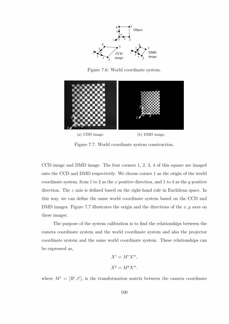
12

34

12

34

1 2

34

y

x

o

CCD

image

DMD

image

oo

xx

y y

Object

z

z z

Figure 7.6: World coordinate system.

x

y

z o

(a) CDD image.

x

y

z o

(b) DMD image.

Figure 7.7: World coordinate system construction.

CCD image and DMD image. The four corners 1, 2, 3, 4 of this square are imaged

onto the CCD and DMD respectively. We choose corner 1 as the origin of the world

coordinate system, from 1 to 2 as the x positive direction, and 1 to 4 as the y positive

direction. The z axis is defined based on the right-hand rule in Euclidean space. In

this way, we can define the same world coordinate system based on the CCD and

DMD images. Figure 7.7 illustrates the origin and the directions of the x, y axes on

these images.

The purpose of the system calibration is to find the relationships between the

camera coordinate system and the world coordinate system and also the projector

coordinate system and the same world coordinate system. These relationships can

be expressed as,

Xc = M cXw,

Xp = MpXw.

where M c = [Rc, tc], is the transformation matrix between the camera coordinate

100

uc

vc

o0

c

(u0

c , v0

c)

CCD

(uc , vc)

oc

p

Camera

lens

Camera

optical axis

fc

op

up

vp

o0

p

(u0

p , v0

p)

(up , vp)

Projector

lens

Projector

optical axis

DMD

fp

(xc, yc, zc)(xw, yw, zw)

(xp, yp, zp)

Objectow

xw

yw

zw

Figure 7.8: Structured light system configuration.

system and the world coordinate system and Mp = [Rp, tp], is the transformation

matrix between the projector coordinate system and the world coordinate system,

and Xc = {xc, yc, zc}T , Xp = {xp, yp, zp}T , and Xw = {xw, yw, zw, 1}T are the co-

ordinate matrices for the point p (see Figure 7.8) in the camera, projector, and the

world coordinate systems, respectively. Xc and Xp can be further transformed to

the CCD and DMD image coordinates (uc, vc) and (up, vp) by applying the intrinsic

matrices Ac and Ap because the intrinsic parameters are already calibrated. That is

sc{uc, vc, 1}T = AcXc,

sp{up, vp, 1}T = ApXp.

The extrinsic parameters can be obtained by the same procedures as those for the

intrinsic parameters estimation. The only difference is that only one calibration image

is needed to obtain the extrinsic parameters. The same Matlab toolbox provided by

Bouguet [92] was utilized to obtain the extrinsic parameters. Example extrinsic

101

parameter matrices for the system setup are

M c =

0.016364, 0.999735, −0.016162, −103.435483

0.999345, −0.015831, 0.032549, −108.195130

0.032285, −0.016684, −0.999339, 1493.079405

,

Mp =

0.019757, 0.999619, −0.019294, −82.087351

0.991605, −0.017125, 0.128161, 131.561677

0.127782, −0.021664, −0.991566, 1514.164208

.

7.2.5 Phase-to-coordinate conversion

Real measured object coordinates can be obtained based on the calibrated

intrinsic and extrinsic parameters of the projector and the camera. Three phase-

shifted fringe images and a centerline image are used to reconstruct the geometry of

the surface. In the following, we discuss how to solve for the coordinates based on

these four images.

For each arbitrary point (uc, vc) on the CCD image plane, its absolute phase

can be calculated, which corresponds to a line in the DMD image with the same

absolute phase value. Without loss of generality, the line is assumed to be a vertical

line with up = ζ(φa(uc, vc)). Assuming the world coordinates of the point to be

(xw, yw, zw), we have the following equation that transform the world coordinates to

the camera image coordinates:

s{ uc vc 1 }T = P c{ xw yw zw 1 }T , (7.13)

where P c is the calibrated matrix for the camera,

P c = AcM c =

αc, γc, uc0

0, βp, vc0

0, 0, 1

rc00 rc

01 rc02 tc0

rc10 rc

11 rc12 tc1

rc20 rc

21 rc22 tc2

.

Similarly, we have the coordinate transformation equation for the projector,

s{ up vp 1 }T = P p{ xw yw zw 1 }T , (7.14)

102

where P p is the calibrated matrix for the projector,

P p = ApMp =

αp, γp, up0

0, βp, vp0

0, 0, 1

rp00 rp

01 rp02 tp0

rp10 rp

11 rp12 tp1

rp20 rp

21 rp22 tp2

.

From Equations 7.13 and 7.14, we can obtain three linear equations,

f1(xw, yw, zw, uc) = 0, (7.15)

f2(xw, yw, zw, vc) = 0, (7.16)

f3(xw, yw, zw, up) = 0. (7.17)

where uc, vc, and up are known. Therefore the world coordinates (xw, yw, zw) of the

point p can be uniquely solved for the image point (uc, vc) (see Appendix A for

details).

7.3 Experiments

To verify the calibration procedures introduced in this chapter, we measured a

planar board with a white surface. The measurement result is shown in Figure 7.9(a).

We then fit the measured coordinates with an ideal flat plane and find the distances

between the measured points and the ideal plane, which are regarded as the mea-

surement error, as illustrated in Figure 7.10. Our experiments show that the error

map has similar patterns for all measured positions and orientations. To compensate

for this type of systematic error, we create an error map LUT based on one position

and then subtract this error map from all the other measurements. As a result, the

measurement accuracy is significantly increased (see details in Section 7.5 ). Fig-

ure 7.10(a) shows the error map before compensation, which is approximately RMS

0.41 mm. After this error compensation, the error is reduced to RMS 0.10 mm as

illustrated in Figure 7.10(b). The remaining error is caused mostly by the residual

non-sinusoidal fringe images. In addition, we measured a sculpture Zeus and the

result is shown in Figure 7.11. The first image is the object with texture mapping,

the second image is the 3D model of the sculpture in shaded mode, and the last one

103

(a) 3D plot of the measured result. (b) Measurement error.

Figure 7.9: 3D measurement result of a planar surface.

−0.5

0

0.5

1

1.5

x(pixel)

y(pi

xel)

50 100 150 200 250 300 350 400 450

50

100

150

200

250

300

350

400

450

500

(a) Error map before compensation.

−0.4

−0.3

−0.2

−0.1

0

0.1

0.2

0.3

0.4

x(pixel)

y(pi

xel)

50 100 150 200 250 300 350 400 450

50

100

150

200

250

300

350

400

450

500

(b) Error map after compensation.

Figure 7.10: Measurement error after calibration.

is the zoom-in view of the 3D model. The reconstructed 3D model is very smooth

with details.

7.4 Calibration Evaluation

For more rigorous evaluation of this calibration procedure, we measured a pla-

nar white board at 12 different positions and orientations as shown in Figure 7.12.

The whole volume is approximately 342 × 376 × 658 mm. The normals, x, y, z

ranges, and the corresponding errors of the plane for each pose are listed in Ta-

ble 7.1. We found that the error of the calibration method did not depend on the

104

(a) 2D photo. (b) 3D shaded. (c) 3D with texture mapping.

Figure 7.11: 3D Measurement result of sculpture Zeus.

orientation of the measured plane unless the plane is positioned far away from thesys-

tem. Figure 7.13(a) illustrates the relationship between the error and the location of

the testing plane. It is obvious that the error is affected by the position of the testing

plane. though it is affected when the plane is put far behind. Figures 7.13(c)-7.13(b)

show the measured error correlated to the rotation angle between x, y, and z axes,

respectively. No clear correlation between the orientation of the testing plane and

the measured error can be observed. Our experiments also show that the remaining

error is mostly caused by the residual non-sinusoidal fringes. Therefore, these results

demonstrate that the calibration is robust and accurate over a large volume.

105

−500 −400 −300 −200 −100 0 100 200 300−500

0

500−100

−50

0

50

100

150

200

250

300

# 5# 6# 7

# 4# 12

# 1# 2# 3

z(mm)

# 11# 8# 9# 10

y(mm)

x(m

m)

Figure 7.12: Positions and orientations of the planar board for the evaluation of thecalibration results.

106

Tab

le7.

1:M

easu

rem

ent

dat

aof

the

test

ing

pla

ne

atdiff

eren

tpos

itio

ns

and

orie

nta

tion

s

Pla

ne

Nor

mal

xra

nge

yra

nge

zra

nge

RM

Ser

ror

RM

S*

erro

r(m

m)

(mm

)(m

m)

(mm

)(m

m)

(mm

)

#1

(-0.

1189

,0.

0334

,0.

9923

)[-32

.55,

236.

50]

[-58

.60,

238.

81]

[-43

.47,

-1.4

7]0.

100.

48#

2(-

0.36

60,0.

0399

,0.

9297

)[-36

.05,

234.

77]

[-64

.24,

243.

10]

[-10

2.24

,14

.61]

0.10

0.33

#3

(-0.

5399

,0.

0351

,0.

8410

)[-40

.46,

234.

93]

[-72

.86,

248.

25]

[-17

2.84

,11

.61]

0.13

0.22

#4

(0.1

835,

0.02

43,0.

9827

)[-60

.11,

233.

74]

[-60

.11,

233.

74]

[-22

.37,

33.3

1]0.

100.

64#

5(0

.198

1,0.

0259

,0.

9798

)[-17

.52,

217.

04]

[-38

.04,

221.

09]

[156

.22,

209.

44]

0.11

0.61

#6

(-0.

1621

,0.

0378

,0.

9860

)[-22

.33,

216.

39]

[-37

.42,

226.

71]

[122

.37,

171.

38]

0.11

0.46

#7

(-0.

5429

,0.

0423

,0.

8387

)[-27

.41,

212.

85]

[-47

.36,

232.

86]

[38.

06,20

2.34

]0.

100.

17#

8(-

0.05

08,0.

0244

,0.

9984

)[-50

.66,

272.

30]

[-96

.88,

260.

18]

[-33

6.22

,-3

10.5

3]0.

220.

55#

9(-

0.05

55,0.

0149

,0.

9983

)[-56

.38,

282.

45]

[-10

8.03

,26

6.72

][-42

5.85

,-4

00.5

4]0.

220.

57#

10(-

0.34

42,0.

0202

,0.

9387

)[-57

.74,

273.

35]

[-10

6.63

,26

8.37

][-44

8.48

,-3

22.4

4]0.

220.

44#

11(0

.485

5,-0

.000

0,0.

8742

)[-43

.70,

281.

07]

[-10

6.88

,26

0.01

][-39

4.84

,-2

14.8

5]0.

200.

67#

12(0

.521

7,-0

.003

7,0.

8531

)[-31

.12,

256.

75]

[-81

.14,

245.

23]

[-1

85.5

1,-1

0.41

]0.

160.

66

Not

e:R

MS

isth

est

anda

rdde

viat

ion

ofth

em

easu

red

plan

eus

ing

our

calib

rati

onm

etho

dR

MS*

isth

est

anda

rdde

viat

ion

ofth

em

easu

red

plan

eus

ing

the

appr

oxim

ate

calib

rati

onm

etho

din

trod

uced

inC

hapt

er3.

107

As a comparison, we compute planar error when the approximate calibration

method introduced in Chapter 3 is employed. Figure 7.14(a) shows the correlation

between the error and the position of the plane. Since the surface normal direction

changes, it may still cause large error. Figures 7.14(c)-7.14(b) show the correlation

between the error and the rotation angle of the plane about x, y, and z axes, re-

spectively. It is obvious that the error is not sensitive to the position but is highly

sensitive to the rotation about of the plane around y axis. This is not desirable for a

real object, the geometry may be complex and the surface normal may vary dramat-

ically from point to point. However, since the approximate calibration method does

not require the additional centerline image, it is suitable for our real-time acquisition,

reconstruction, and display system. Even though, the error is larger (RMS 0.6 mm),

it is still acceptable for a real-time system.

To further verify that our calibration method is not significantly affected by the

surface normal direction while the traditional method is, we measured a cylindrical

surface with a diameter of 200 mm. Figure 7.15 shows the measurement results. In

comparison with the measurement result obtained using the traditional approximate

calibration method, the error is significantly smaller. This is because the surface

normal of a cylindrical surface changes continuously across the surface and the tra-

ditional approximate calibration method is highly sensitive to this change.

7.5 Discussion

The calibration method introduced in this research for the structured light

systems has the following advantages over other methods:

• Simple The proposed calibration method separates the projector and camera

calibration, which makes the calibration simple.

• Simultaneous For each checkerboard calibration pose, the camera image and

the projector image can be obtained simultaneously. Therefore, the camera

and the projector can be calibrated simultaneously.

• Fast The calibration of the projector and the camera follows the same pro-

108

−500 −400 −300 −200 −100 0 100 2000.08

0.1

0.12

0.14

0.16

0.18

0.2

0.22

z (mm)

Err

or R

MS

(m

m)

(a)

0 5 10 15 20 25 30 350.08

0.1

0.12

0.14

0.16

0.18

0.2

0.22

Angle between z axis(degree)

Err

or R

MS

(m

m)

(b)

50 60 70 80 90 100 110 120 1300.08

0.1

0.12

0.14

0.16

0.18

0.2

0.22

Angle between x axis(degree)

Err

or R

MS

(m

m)

(c)

87.5 88 88.5 89 89.5 90 90.50.08

0.1

0.12

0.14

0.16

0.18

0.2

0.22

Angle between y axis(degree)

Err

or R

MS

(m

m)

(d) .

Figure 7.13: Planar error correlated to the poses of the measured plane using ourcalibration method. (a) Planar error vs plane position. (b) Planar error plane rota-tion angel around x axis. (c) Planar error vs plane rotation angel around y axis. (d)Planar error vs plane rotation angel around z axis.

cedures of camera calibration. A standard checkerboard can be utilized to

calibrate the camera and the projector simultaneously. This is much faster

than other structured light calibration methods in which complex optimiza-

tion procedures have to be involved to obtain the relationship between the

camera and projector parameters.

• Accurate Since the projector and camera calibrations are independent, there

is no coupling issue involved and thus more accurate parameters of the cam-

era and projector can be obtained.

For the system we developed, we did not use the nonlinear model for the camera

or the projector. Our experiments showed that the nonlinear model generates worse

109

−500 −400 −300 −200 −100 0 100 2000.1

0.2

0.3

0.4

0.5

0.6

0.7

0.8

z (mm)

RM

S e

rror

(m

m)

(a)

0 5 10 15 20 25 30 350.1

0.2

0.3

0.4

0.5

0.6

0.7

0.8

Angle(degree)

RM

S e

rror

(m

m)

(b)

50 60 70 80 90 100 110 120 1300.1

0.2

0.3

0.4

0.5

0.6

0.7

0.8

Angle(degree)

RM

S e

rror

(m

m)

(c)

87.5 88 88.5 89 89.5 90 90.50.1

0.2

0.3

0.4

0.5

0.6

0.7

0.8

Angle (degree)

RM

S e

rror

(m

m)

(d)

Figure 7.14: Planar error correlated to the poses of the measured plane using tra-ditional approximate calibration method. (a) Planar error vs plane position. (b)Planar error plane rotation angel around x axis. (c) Planar error vs plane rotationangel around y axis. (d) Planar error vs plane rotation angel around z axis.

results since the nonlinear distortion of the lenses of our system was small. Use

of the nonlinear model may have caused numerical instability. To verify that the

nonlinear distortions of the camera and the projector are negligible, we compute the

errors of the corner points of the checkerboard on the image planes of the camera and

projector assuming a linear model. Here the error is defines as the difference between

the coordinates of a checker corner point as computed from the real captured image

and from the back projected image based on a linear model. Figure 7.16 shows the

error for the calibration plane, whose variations are within one pixel. Therefore the

linear model is sufficient to describe the camera and the projector of our system.

110

50 100 150 2000

20

40

60

80

100

x (mm)

z (m

m)

Measured dataIdeal data

(a)

50 100 150 200−100

−80

−60

−40

−20

0

x (mm)

z (m

m)

Measured dataIdeal data

(b)

50 100 150 200−2

−1

0

1

2

3

4

5

6

x (mm)

z er

ror

(mm

)

(c)

50 100 150 200−2

−1

0

1

2

3

4

5

6

x (mm)

z er

ror

(mm

)

(d)

Figure 7.15: Measurement result of a cylinder. (a) Cross section of the measuredshape using our calibration method. (b) Cross section of the measured shape usingthe approximate calibration method. (c) Shape error for our calibration. (d) Shapeerror for the traditional approximate calibration method.

7.6 Conclusions

This chapter introduced a novel structured light calibration method that cali-

brates the projector and the camera independently and accurately. The measurement

error is demonstrated to be RMS 0.22 mm over a volume of 342 × 376 × 658 mm.

We proposed a method that enabled a projector “capture” images, thus turning the

projector into a bi-directional device which might have potential other applications in

computer graphics, medical imaging, plastic surgery, etc. The calibration is fast, ro-

bust and accurate. It, significantly simplifies the structured light system calibration

and re-calibration procedures.

111

−1 −0.5 0 0.5 1

−0.8

−0.6

−0.4

−0.2

0

0.2

0.4

0.6

0.8

Reprojection error (in pixel)

x

y

(a) Error for the projector.

−0.8 −0.6 −0.4 −0.2 0 0.2 0.4 0.6 0.8

−0.6

−0.4

−0.2

0

0.2

0.4

0.6

0.8

Reprojection error (in pixel)

x

y

(b) Error for the camera.

Figure 7.16: Error caused by nonlinear image distortions.

112

Chapter 8

Conclusions and Future Works

This chapter summarizes the accomplishments and proposes the future works

of this dissertation research.

8.1 Conclusions

In this dissertation research, we made the following major contributions:

(1) Developed an advanced high-resolution, real-time 3D shape mea-

surement system

Two high-resolution, real-time 3D shape measurement systems have been

successfully developed in this research. Both systems generate a data cloud

of 532× 500 points per frame. The first system has a speed of 40 frames per

second for 3D data acquisition, 40 frames per second for B/W texture image

acquisition, and 26.7 frames per second for color texture image acquisition.

The second system has a lower speed of 30 frames per second for both 3D

data and B/W texture image acquisition. Color texture mapping is not

possible for the second system due to hardware limitation. However, the

second system is much more stable and produces better results with smaller

errors, as compared to the first system. By further implementing the fast 3D

reconstruction algorithms and parallel processing technique into the real-time

3D data acquisition system, we developed a system that can simultaneously

acquire, reconstruct and display 3D information of the measured object at a

113

frame rate of up to 40 frames per second and at a image resolution of 532 ×500 points per frame. Experiments demonstrated that the real-time system

provided satisfactory measurement results for slow moving objects such as

human facial expressions.

(2) Developed a novel trapezoidal phase-shifting method

A novel coding algorithm, trapezoidal phase-shifting algorithm was devel-

oped in this research. It has the advantage of high computation speed,

which is at least 4.5 times faster when compared to the traditional sinusoidal

phase-shifting method. If compared with the intensity ratio based methods,

this algorithm is significantly less sensitive to image defocus, thus permitting

a larger dynamic range measurement. This coding algorithm made real-time

3D reconstruction possible at an image resolution of 532 × 500 pixels with

an ordinary PC (Pentium 4, 2.8 GHz).

(3) Developed a novel fast phase-wrapping algorithm

Though the trapezoidal phase-shifting algorithm is much less sensitive to

image defocus as compared to the intensity ratio based methods, it is still

affected by the defocusing effect. In the extreme case, when the trapezoidal

fringe pattern is defocused so much that it becomes sinusoidal, we found that

the error was still at a relatively small value of 0.6%. Based on this finding, we

introduced a fast phase-wrapping algorithm which employs the trapezoidal

phase-shifting algorithm to process sinusoidal patterns and a LUT method

to compensate for the error. The reconstructed geometry has similar quality

as that of the traditional phase-wrapping algorithm. This new algorithm

combines the speed advantage of the trapezoidal phase-shifting algorithm

and the accuracy advantage of the sinusoidal phase-shifting algorithm. By

implementing this new algorithm, 3D reconstruction can be accomplished in

real time with high accuracy.

(4) Developed a novel error compensation method

114

In the phase-shifting method we used, the distortion of the supposedly sinu-

soidal fringe patterns due to projector nonlinearity is the major error source.

In this research, a novel method was developed that could theoretically com-

pletely eliminate the error caused by the non-sinusoidal waveforms. This

method uses a small LUT to compensate for the error and was shown to be

able to reduce the error by 10 times. In addition, a method was developed to

correct the non-sinusoidality of the fringe patterns, which makes high-quality

texture mapping possible. Texture mapping important for applications in

computer vision and computer graphics.

(5) Developed a novel calibration method

A novel method was developed for accurate and quick system calibration. In

particular, a new method was developed that enabled a projector to “cap-

ture” images like a camera, thus making the calibration of a projector the

same as that of a camera. This is a significant development because today

projectors are increasingly used in various measurement systems yet so far no

systematic way of calibrating them has been developed. With the proposed

method, the total calibration process only took approximately 30 minutes.

Our experimental results demonstrated that the measurement accuracy of

our system was less than RMS 0.22 mm over a volume of 342 × 376 × 658

mm.

8.2 Future Works

In this research, we successfully developed two prototype real-time 3D shape

measurement systems. However, there are still many research issues to be studied

and applications to be explored.

(1) Eliminate errors caused by tangent illumination

When the projection light is tangent to an object’s surface, the spatial fringe

period becomes infinite, which causes phase distortion and therefore mea-

surement error. Figure 8.1 shows a typical case when large errors occur near

115

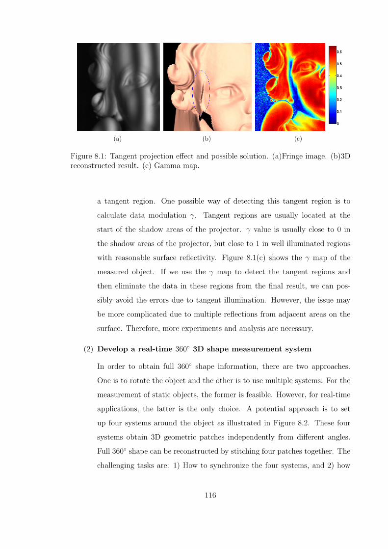
(a) (b) (c)

Figure 8.1: Tangent projection effect and possible solution. (a)Fringe image. (b)3Dreconstructed result. (c) Gamma map.

a tangent region. One possible way of detecting this tangent region is to

calculate data modulation γ. Tangent regions are usually located at the

start of the shadow areas of the projector. γ value is usually close to 0 in

the shadow areas of the projector, but close to 1 in well illuminated regions

with reasonable surface reflectivity. Figure 8.1(c) shows the γ map of the

measured object. If we use the γ map to detect the tangent regions and

then eliminate the data in these regions from the final result, we can pos-

sibly avoid the errors due to tangent illumination. However, the issue may

be more complicated due to multiple reflections from adjacent areas on the

surface. Therefore, more experiments and analysis are necessary.

(2) Develop a real-time 360◦ 3D shape measurement system

In order to obtain full 360◦ shape information, there are two approaches.

One is to rotate the object and the other is to use multiple systems. For the

measurement of static objects, the former is feasible. However, for real-time

applications, the latter is the only choice. A potential approach is to set

up four systems around the object as illustrated in Figure 8.2. These four

systems obtain 3D geometric patches independently from different angles.

Full 360◦ shape can be reconstructed by stitching four patches together. The

challenging tasks are: 1) How to synchronize the four systems, and 2) how

116

Projector 1

Object

System 1

System 4

System 3

System 3

Figure 8.2: Full field real-time 3D measurement system.

to stitch four patches automatically and accurately.

(3) Explore applications of projectors as bi-directional devices

In this research, we found a way to allow a projector to “capture” images

with the assistance of a camera. Therefore we have essentially converted

a projector into a bi-directional device, which projects images as a normal

projector and “captures” images like a camera. The potential applications

of this device are extensive, including entertainment, plastic surgery, online

assembly, etc., and should be explored.

(4) Explore more applications

This real-time system developed in this research has many potential ap-

plications, such as medical imaging, security, facial recognition, design and

manufacturing, etc. During the course of this dissertation research, we have

worked with other researchers to explore the applications of our real-time

systems in the areas of computer vision and computer graphics, in partic-

117

ular human facial expression analysis and modeling, and facial recognition.

We plan to continue this collaboration and in the mean time, explore more

applications in other areas, especially biomedical.

118

Appendix A

World Coordinates Calculation

For the camera and projector, let’s assume intrinsic matrices are Ac, Ap respec-

tively. Extrinsic parameter matrices are [Rc, tc] and [Rp, tp] respectively. Assume

X = {xw, yw, zw}T (A.1)

is the world coordinates, and

Ic = {uc, vc, 1}T

and

Ip = {up, vp, 1}T

are image coordinates of the camera and projector respectively. Then we have,

scIc = Ac[Rc, tc]{X, 1}T (A.2)

= AcRcX + Actc (A.3)

= BcX + dc (A.4)

where Bc = AcRc, dc = AcT c

spIp = BpX + dp (A.5)

here Bp = ApRp, dp = ApT p

scIci =

k=1∑3

(BcikX

k) + dci (A.6)

spIpi =

k=1∑3

(BpikX

k) + dpi (A.7)

119

here i = 1, 2, 3, where the superscript means the element of the vector. Ic1 is the first

element of vector Ic. The following notation follows the same definition. Then we

have,

AX = b (A.8)

where A is a 3 × 3 matrix, and b is a 3 × 1 vector, Assume we know the horizontal

line position of the corresponding pixels, then,

Aij = Bc3jI

ci −Bc

ij (A.9)

A3j = Bp3jI

p1 −Bp

1j (A.10)

here i = 1, 2, 3, j = 1, 2. Where Bcij is the i− th row, j− th column element of matrix

Bc.

bj = dcj −Bc

3jdc3 (A.11)

b3 = dp3 −Bp

32dp3 (A.12)

Then

X = A−1b

120

Bibliography

[1] U. Dhond and J. Aggarwal, “Structure from Stereo-A Review,” IEEE Trans.Systems, Man, and Cybernetics 19(6), 1489–1510 (1989).

[2] R. Zhang, P.-S. Tsai, J. Cryer, and M. Shah, “Shape from Shading: A Sur-vey,” IEEE Trans. on Pattern Analysis and Machine Intelligence 21(8), 690–706(1999).

[3] M. Subbarao and T. Choi, “Focusing Techniques,” in Proc. of SPIE, pp. 163–174(1992).

[4] M. Subbarao and G. Surya, “Application of Spatial-Domain Convolu-tion/Deconvolution Transform for Determing Distance from Image Defocus,”in Proc. of SPIE, pp. 159–167 (1992).

[5] M. Levoy, K. Pulli, B. Curless, S. Rusinkiewicz, D. Koller, L. Pereira, M. Ginz-ton, S. Anderson, J. Davis, J. Ginsberg, J. Shade, and D. Fulk, “The Digi-tal Michelangelo Project,” in Proceedings of SIGGRAPH 2000, K. Akeley, ed.,Computer Graphics Proceedings, Annual Conference Series, pp. 131–144, ACM(ACM Press / ACM SIGGRAPH, 2000).

[6] J. Batlle, E. M. Mouaddib, and J. Salvi, “Recent Progress in Coded StructuredLight as a Technique to Solve the Correspondence Problem: A Survey,” PatternRecognition pp. 1–63 (1998).

[7] B. Curless, “Overview of Active Vision Techniques,” in Proc. SIGGRAPH 99Course on 3D Photography (1999).

[8] J. Davis, R. Ramamoorthi, and S. Rusinkiewicz, “Spacetime Stereo: A UnifyingFramework for Depth from Triangulation,” IEEE Trans. on Pattern Analysis andMachine Intelligence 27(2), 1–7 (2005).

[9] G. Hobrough and T. Hobrough, “Stereopsis for Robots by Iterative Stereo ImageMatching,” in Proc. SPIE, vol. 449 of Intelligent Robots: 3rd Intl Conf on RobotVision and Sensory Controls, pp. 94–102 (1983).

[10] A. Fusiello, V. Roberto, and E. Trucco, “Efficient Stereo with Multiple Window-ing,” in IEEE Int’l Conference on Computer Vision and Pattern Recognition,pp. 858–863 (1997).

121

[11] R. C. Gonzalez and R. E. Woods, Digital Image Processing (Addison Wesly,1992).

[12] C. Sun, “A Fast Stereo Matching Method,” in Digital Image Computing: Tech-niques and Applications, pp. 137–148 (1997).

[13] J. Weng, N. Ahuia, and T. S. Huang, “Matching Two Perspective Views,” IEEETrans. on Pattern Analysis and Machine Intelligence 14, 917–924 (1992).

[14] P. J. Burt, “The Laplacian Pyramid as a Compact Image Code,” IEEE Trans.on Communications 31(4), 532–540 (1983).

[15] A. Koschan and V. Rodehorst, “Dense Depth Map by Active Color Illuminationand Image Pyramids,” in Advances in Computer Vision, pp. 137–148 (1997).

[16] L. Zhang, B. Curless, and S. Seitz, “Spacetime Stereo: Shape Recovery forDynamic Senses,” in Proc. Copmuter Vison and Pattern Recognition (2003).

[17] C. S. Fraser, “Photogrammetric Measurement to One Part in a Million,” Pho-togramm. Eng. Remote Sens. 58(3), 305–310 (1992).

[18] B. K. P. Horn and M. J. Brooks, Shape from Shading (MIT Press, Cambridge,MA, 1989).

[19] R. A. Jarvis, “A Perspective on Range Finding Techniques for Computer Vi-sion,” IEEE Trans. Pattern Analysis and Machine Intelligence 5(2), 122–139(1983).

[20] E. Krotkov, “Focusing,” Int’l J. of Computer Vision 1, 223–237 (1987).

[21] J. S. Massa, G. S. Buller, A. C. Walker, S. Cova, M. Umasuthan, and A. M.Wallace, “Time of Flight Optical Ranging System Based on Time-CorrelatedSingle-Photo Counting,” Appl. Opt. 37(31), 7298–7304 (1998).

[22] P. Besl, “Active Optical Range Imaging Sensor,” Machine Vision and Applica-tions 1, 127–152 (1988).

[23] Z. Ji and M. C. Leu, “Design of Optical Triangulation Devices,” Opt. LaserTechnology 21(5), 335–338 (1989).

[24] C. P. Keferstein and M. Marxer, “Testing Bench for Laser Triangulation Sen-sors,” Sens. Rev. 18(3), 183–187 (1998).

[25] J. L. Posdamer and M. D. Altschuler, “Surface Measurement by Space-encodedProjected Beam Systems,” Computer Graphics and Image Processing 18(1),1–17 (1982).

[26] D. Skocaj and A. Leonardis, “Range Image Acquisition of Objects with Non-uniform Albedo Using Structured Light Range Sensor,” in IEEE Proc. of the15th International Conference on Pattern Recognition, vol. 1, pp. 778–781(2000).

122

[27] J. Salvi, J. Pages, and J. Batlle, “Pattern codification strategies in structuredlight systems,” Pattern Recognition 37(4), 827–849 (2004).

[28] J. Pan, P. Huang, S. Zhang, and F.-P. Chiang, “Color N-ary Gray Code For 3-DShape Measurement,” in Proc. 12th Int’l Conference on Experimental Mechanics(2004).

[29] D. Caspi, N. Kiryati, and J. Shamir, “Range Imaging with Adaptive ColorStructured Light,” IEEE Trans. on Pattern Analysis and Machine Intelligence20(5), 470–480 (1998).

[30] E. Horn and N. Kiryati, “Toward Optimal Structured Light Patterns,” Imageand Vision Computing 17(2), 87–89 (1999).

[31] B. Carrihill and R. Hummel, “Experiments with the Intensity Ratio Depth Sen-sor,” Computer Vision, Graphics and Image Processing 32, 337–358 (1985).

[32] T. Miyasaka, K. Kuroda, M. Hirose, and K. Araki, “Reconstruction of Realistic3D Surface Model and 3D Animation from Range Images Obtained by Real Time3D Measurement System,” in IEEE 15th International Conference on PatternRecognition, pp. 594–598 (2000).

[33] G. Chazan and N. Kiryati, “Pyramidal Intensity-Ratio Depth Sensor,” Tech.Rep. No. 121, Israel Institute of Technology, Technion, Haifa, Israel (1995).

[34] S. Savarese, J. Bouguet, and P. Perona, “3D Depth Recovery with GrayscaleStructured Lighting,” Tech. rep., Computer Vision, California Insititute of Tech-nology (1998).

[35] K. A. Haines and B. P. Hildebrand, “Contour Generation by Wavefront Con-struction,” Phys. Lett. 19, 10–11 (1965).

[36] K. Creath, Y. Y. Cheng, and J. Wyant, “Contouring Aspheric Surface UsingTwo-Wavelength Phase Shifting Interferometry,” Opt. Acta. 32(12), 1455–1464(1985).

[37] R. P. Tatam, J. C. Davies, c. H. Buckberry, and J. D. C. Jones, “HolographicSurface Contouring Using Wavelength Modulation of Laser Diode,” Opt. LaserTechnol. 22, 317–321 (1990).

[38] J. S. Zelenka and J. R. Varner, “Multiple-index Holographic Contouring,” Appl.Opt. 9(2), 1431–1434 (1969).

[39] Y. Y. Hung, J. L. Turner, M. Tafralian, J. D. Hovanesian, and C. E. Taylor,“Optical Method for Measuring Contour Slopes of an Object,” Appl. Opt. 17(1),128–131 (1978).

[40] H. Ei-Ghandoor, “Tomographic Investigation of the Refractive Index ProfilingUsing Speckle Photography Technique,” Opt. Commun. 133, 33–38 (1997).

123

[41] C. Joenathan, B. Fraze, P. Haible, and H. J. Tiziani, “Contouring by ElectronicSpeckle Pattern Interferometry Using Dual Beam Illumination,” Appl. Opt. 29,1905–1911 (1990).

[42] R. Rodrfguez-Vera, D. Kerr, and F. Mondoza-Santoyo, “Electronic Speckle Con-touring,” J. Opt. Soc. Am. A 9(1), 2000–2008 (1992).

[43] L. S. Wang and S. Krishnaswamy, “Shape Measurement Using Additive-Subtractive Phase Shifting Speckle Interferometry,” Meas. Sc. Technol. 7, 1748–1754 (1996).

[44] F. Chen, G. M. Brown, and M. Song, “Overview of Three-Dimensional ShapeMeasurement Using Optical Method,” Opt. Eng. 39(1), 10–22 (2000).

[45] F. P. Chiang, “Techniques of Optical Spatial Filtering Applied to the Processingof Moire -Fringe Patterns,” Experimental Mechanics pp. 523–526 (1969).

[46] Y. Z. Dai and F. P. Chiang, “Moire Interferometry Applied to TopographicContour Measurement,” in Proc. SPIE, vol. 954 of Optical Testing and MetrologyII, pp. 153–157 (1988).

[47] M. Idesawa, T. Yatagai, and T. Soma, “Scanning Moire Method and AutomaticMeasurement of 3-D Shapes,” Appl. Opt. 16(8), 2153–2162 (1977).

[48] V. Srinivasan, L. H. C., and M. Halioua, “Automated Phase-Measuring Pro-filometry of 3D Diffuse Objects,” Appl. Opt. 23(18), 3105–3108 (1984).

[49] H. Takasaki, “Moire Topography,” Appl. Opt. 9(6), 1467–1472 (1970).

[50] A. J. Boehnlein and K. G. Harding, “Adaptation of a Parallel Architecture Com-puter to Phase-shifted Moire Interferometry,” in Proc. SPIE, vol. 728 of Optics,Illumination, and Image Sensing for machine Vision, pp. 183–194 (1986).

[51] M. Halioua and H.-C. Liu, “Optical Three-Dimension Sensing by Phase Mea-suring Profilometry,” Opt. and Lasers in Engineering 11, 185–215 (1989).

[52] H. P. Stahl, “White-light Moire Phase-measuring Interferometry,” in Proc.SPIE, vol. 1332 of Optical Testing and Metrology III: Recent advances in in-dustrial optical inspection, pp. 720–728 (1990).

[53] L. H. Bieman, “Survey of Design Consideration for 3D Imaging System,” inProc. SPIE, vol. 1005 of Optics, illumination, and image sensing for machinevision III, pp. 138–144 (1988).

[54] K. G. Harding and J. S. Harris, “Projection Moire Interferometry for VibrationAnalysis,” Appl. Opt. 22(6), 856–861 (1983).

[55] C. Reich, R. Rtter, and J. Thesing, “3-D Shape Measurement of Complex Objectby Combining Photogrammetry and Fringe Projection,” Opt. Eng. 39(1), 224–230 (2000).

124

[56] W. Schreiber and G. Notni, “Theory and Arrangements of Self-calibratingWhole-body Three-dimensional Measurement Systems Using Fringe ProjectionTechnique,” Opt. Eng. 39(1), 159–169 (2000).

[57] K. G. Harding, “Phase Grating Use for Slop Discrimination in Moire Contour-ing,” in Proc. SPIE, vol. 1614 of Optics, illumination, and image sensing formachine vision VI, pp. 265–270 (1991).

[58] Z. J. Geng, “Rainbow 3-D Camera: New Concept of High-Speed Three VisionSystem,” Opt. Eng. 35, 376–383 (1996).

[59] C. Wust and D. W. Capson, “Surface Profile Measurement using Color FringeProjection,” Machine Vision and Applications 4, 193–203 (1991).

[60] P. S. Huang, Q. Hu, F. Jin, and F. P. Chiang, “Color-Encoded Digital FringeProjection Technique for High-Speed Three-Dimensional Surface Contouring,”Opt. Eng. 38, 1065–1071 (1999).

[61] L. Zhang, B. Curless, and S. M. Seitz, “Rapid Shape Acquisition Using ColorStructured Light and Multi-pass Dynamic Programming,” in The 1st IEEE In-ternational Symposium on 3D Data Processing, Visualization, and Transmis-sion, pp. 24–36 (2002).

[62] M. Takeda and K. Mutoh, “Fourier Transform Profilometry for the AutomaticMeasurement of 3-D Object Shape,” Appl. Opt. 22(24), 3977–3982 (1983).

[63] S. Rusinkiewicz, O. Hall-Holt, and L. Marc, “Real-Time 3D Model Acquisition,”in SIGGRAPH, vol. 1281 of 3D acquisition and image based rendering, pp. 438– 446 (ACM Press, 2002).

[64] O. Hall-Holt and S. Rusinkiewicz, “Stripe Boundary Codes for Real-TimeStructured-Light Range Scanning of Moving Objects,” in The 8th IEEE In-ternational Conference on Computer Vision, pp. II: 359–366 (2001).

[65] P. S. Huang, C. Zhang, and F. P. Chiang, “High-Speed 3-D Shape MeasurementBased on Digital Fringe Projection,” Opt. Eng. 42(1), 163–168 (2003).

[66] L. J. Hornbeck, “Current Status of the Digital Micromirror Device (DMD) forProjection Television Applications,” in Intl. Electron. Devices Tech. Digest, pp.381–384 (1993).

[67] J. M. Younse, “Mirrors on a Chip,” in IEEE Spectrum, pp. 27–31 (1993).

[68] D. Malacara, ed., Optical Shop Testing (John Wiley and Songs, NY, 1992).

[69] D. C. Ghiglia and M. D. Pritt, Two-Dimensional Phase Unwrapping: Theory,Algorithms, and Software (John Wiley and Sons, Inc, 1998).

125

[70] W. H. Press, B. P. Flannery, S. A. Teukolsky, and W. T. Vetterling, NumericalRecipes in C: the Art of Scientific Computing, 2nd ed. (University of Cambridge,Cambridge, 1992).

[71] C. Zhang, “Optical Profilometry and its Applications,” Ph.D. thesis, State Uni-versity of New York at Stony Brook, Stony Brook, NY, 11794 (2001).

[72] J. H. Brunning, J. E. Herriott, D. P. Gallagher, A. White, and D. J. Brangaccio,“Digital Wavefront Measuring Interferometer for Testing Optical Surfaces andLenses,” Appl. Opt. 13, 2693–2073 (1974).

[73] D. Malacara, ed., Optical Shop Testing (John Wiley and Songs, NY, 1992).

[74] P. S. Huang, Q. Y. Hu, , and F. P. Chiang, “Double Three-step Phase-shiftingAlgorithm,” Appl. Opt. 41(22), 4503–4509 (2002).

[75] R. Legarda-Saenz, T. Bothe, and W. P. Juptner, “Accurate Procedure for theCalibration of a Structured Light System,” Opt. Eng. 43(2), 464–471 (2004).

[76] F. J. Cuevas, M. Servin, and R. Rodriguez-Vera, “Depth Object Recovery UsingRadial Basis Functions,” Opt. Commun 163(4), 270–277 (1999).

[77] F. J. Cuevas, M. Servin, O. N. Stavroudis, and R. Rodriguez-Vera, “Multi-layerNeural Networks Applied to Phase and Depth Recovery From Fringe Patterns,”Opt. Commun 181(4), 239–259 (2000).

[78] C. C. Slama, C. Theurer, and S. W. Henriksen, Manual of Photogrammetry,American Society of Photogrammetry, 4th ed. (Falls Church, VA, 1980).

[79] C. S. Fraser, “Photogrammetric Camera Component Calibration: A Review ofAnalytical Techniques,” in Calibration and Orientation of Camera in ComputerVision, A. Gruen and T. S. Huang, eds., pp. 95–136 (Springer-Verlag, BerlinHeidelberg, 2001).

[80] A. Gruen and H. A. Beyer, “System Calibration Through Self-Calibration,” inCalibration and Orientation of Camera in Computer Vision, A. Gruen and T. S.Huang, eds., pp. 163–194 (Springer-Verlag, Berlin Heidelberg, 2001).

[81] J. Heikkila, “Geometric Camera Calibration Using Circular Control,” IEEETrans. Pattern Anal. Mach. Iintell. PAMI-22(10), 1066–1077 (2000).

[82] F. Pedersini, A. Sarti, and S. Tubaro, “Accurate and Simple Geometric Cali-bration of Multi-camera Systems,” Signal Process 77(3), 309–334 (1999).

[83] D. B. Gennery, “Least-square Camera Calibration Including Lens Distortionand Automatic Editing of Calibration Points,” in Calibration and Orientationof Camera in Computer Vision, A. Gruen and T. S. Huang, eds., pp. 123–136(Springer-Verlag, Berlin Heidelberg, 2001).

126

[84] Q. Hu, P. S. Huang, Q. Fu, , and F. P. Chiang, “Calibration of a 3-D ShapeMeasurement System,” Opt. Eng. 42(2), 487–493 (2003).

[85] D. C. Brown, “Close-range Camera Calibration,” Photogrametric Engineering37(8), 855–866 (1971).

[86] W. Faig, “Calibration of Close-range Photogrammetry System: MathematicalFormulation,” Photogrametric Engineering and Remote Sensing 41(12), 1479–1486 (1975).

[87] C. Slama, Manual of Photogrammetry, 4th ed. (American Society of Photogram-metry, 1980).

[88] J. Weng, P. Cohen, and M. Herniou, “Camera Calibration with Distortion Mod-els and Accuracy Evaluation,” IEEE Trans. on Pattern Analysis and MachineIntelligence 14(10), 965–980 (1992).

[89] R. Y. Tsai, “A Versatile Camera Calibration Technique for High-accuracy 3DMachine Vision Metrology using Off-the-shelf TV Camera and Lenses,” IEEEInt. J. Robot. Automat. RA-3 3(4), 323–344 (1987).

[90] G. Wei and S. Ma, “Implicit and Explicit Camera Calibration: Theory andExperiments,” IEEE Trans. on Pattern Analysis and Machine Intelligence 16(5),469–480 (1994).

[91] Z. Zhang, “A Flexible New Technique for Camera Calibration,” IEEE Trans onPattern Analysis and Machine Intelligence 22(11), 1330–1334 (2000).

[92] J.-Y. Bouguet, “Camera Calibration ToolBox for Matlab,” Online available at:http://www.vision.caltech.edu/bouguetj/calib doc.

127