high resolution imaging ground penetrating radar … · high resolution imaging ground penetrating...
TRANSCRIPT

High Resolution Imaging Ground Penetrating Radar Design and Simulation
Charles Phillip Saunders II
Thesis submitted to the faculty of the Virginia Polytechnic Institute and State
University in partial fulfillment of the requirements for the degree of
Master of Science in Mechanical Engineering
Alfred L. Wicks, Chair
Kathleen Meehan
John P. Bird
10APR2014
Blacksburg, VA
Keywords: High Resolution, Ground Penetrating, Radar, Fundamentals, Concepts, Landmines

High Resolution Imaging Ground Penetrating Radar Design and Simulation
Charles Phillip Saunders II
ABSTRACT
This paper describes the design and simulation of a microwave band, high resolution
imaging ground penetrating radar. A conceptual explanation is given on the mechanics of wave-
based imaging, followed by the governing radar equations. The performance specifications for
the imaging system are given as inputs to the radar equations, which output the full system
specifications. Those specifications are entered into a MATLAB simulation, and the simulation
results are discussed with respect to both the mechanics and the desired performance. Finally,
this paper discusses limitations of the design, both with the simulations and anticipated issues if
the device is fully realized.

iii
PREFACE
This thesis is the result of research in support of an imaging metal detector. I knew that
early radar and sonar systems produced a “ping” that corresponded to the target distance when
the antenna or transducer was pointed in the correct direction. When installed in arrays, those
systems were capable of generating detailed, sometimes photorealistic, images instead of just
“blips” on an operator screen.
I spent a great deal of time trying to grasp the fundamental concepts of how an array
allows a system to produce images. There were, in general, two types of literature that I could
find on array-based imaging: the first group assumed you already knew how imaging worked and
offered advanced processing techniques; and the other, which decided that the best way to
explain imaging is with differential equations and as little supporting explanatory text as
possible.
The very best papers I have read were written in a more relaxed, informal manner, and
attempted to explain the fundamental concepts before or while introducing the governing
mathematics. I believe that a more conversational tone helps to put the reader at ease, and I have
emulated this style in this paper in the hopes that you, the reader, can focus more on what I’m
saying instead of how I’m saying it.
Please feel free to contact me with any questions or feedback regarding this paper. I have
had my civilian email address, “[email protected]”, for nearly a decade now, and intend to
keep it for the foreseeable future. Please be sure to reference radar imaging, or I may mistakenly
regard your message as spam.

iv
ACKNOWLEDGEMENTS
I would like to dedicate this paper to my Grandfather, who died around the time the first
successful simulations were being performed. Words cannot express how much his love and
support meant to me and everyone else in my family. He often said he didn’t understand the finer
points of my research, but he was always eager to hear about the latest progress, shared joy in my
breakthroughs, and offered words of encouragement during my setbacks. He will be sorely
missed.
I would also like to thank my advisors, friends, family, and of course, my wife Kristine ♥

v
TABLE OF CONTENTS
Abstract ...................................................................................................................................... iv
Preface ........................................................................................................................................ iii
Acknowledgements .................................................................................................................... iv
Table of Contents ........................................................................................................................ v
List of Figures .......................................................................................................................... viii
List of Tables ............................................................................................................................... x
Acronymns and Abbreviations ................................................................................................... xi
CHAPTER 1 THESIS PROBLEM DEFINITION AND APPROACH ................................... 1
Chapter Summary ........................................................................................................................ 1
The Landmine Problem ............................................................................................................... 1
Initial Approach........................................................................................................................... 1
Existing Mine Detection Systems ............................................................................................... 2
Performance Requirements - The Need for Something New ...................................................... 6
CHAPTER 2 RADAR MECHANICS CONCEPTUAL DESCRIPTION ................................ 8
Chapter Summary ........................................................................................................................ 8
Isotropic Radiators ...................................................................................................................... 8
Multiple Radiators ....................................................................................................................... 9
Continuous and Discrete Apertures........................................................................................... 12
Beamwidth ................................................................................................................................ 13
Beam Steering ........................................................................................................................... 20
Pulsed vs. Continuous Wave Radar .......................................................................................... 21
Processing the Returned Signal ................................................................................................. 22
Sidelobes and Phantom Images ................................................................................................. 25
Spherical vs. Cartesian Resolution ............................................................................................ 27
Range Resolution ...................................................................................................................... 28
Basic Operation Recap .............................................................................................................. 29
CHAPTER 3 RADAR MECHANICS MATHEMATICAL DESCRIPTION .........................31
Chapter Summary ...................................................................................................................... 31
Performance Metrics ................................................................................................................. 31
Detection and the Signal to Noise Ratio ........................................................................... 31

vi
The Pulse - Range, Range Resolution, Pulse Repetition Frequency and Bandwidth ....... 33
Aperture Size Calculation ......................................................................................................... 34
Beam Width Calculation ........................................................................................................... 35
Operating Frequency Selection ................................................................................................. 36
Transmitter Power Estimation ................................................................................................... 36
Threshold Selection ................................................................................................................... 38
CHAPTER 4 DESIGN CRITERIA, FULL SYSTEM SPECS, AND TARGETS ...................39
Chapter Summary ...................................................................................................................... 39
System Design ........................................................................................................................... 39
Overview ........................................................................................................................... 39
The Minimum Target ........................................................................................................ 40
Operating Frequency ......................................................................................................... 42
Beam Width ...................................................................................................................... 43
Detection Probabilities ...................................................................................................... 43
Antenna Selection ............................................................................................................. 44
Full System Specifications ........................................................................................................ 45
Targets for a Crowded Scene .................................................................................................... 46
Scanning Method and Expected Simulation Results................................................................. 51
CHAPTER 5 SIMULATION RESULTS AND DISCUSSION .............................................56
Chapter Summary ...................................................................................................................... 56
Method of Simulation................................................................................................................ 56
Non-Imaging Specifications ...................................................................................................... 57
Transmission Power .......................................................................................................... 57
Revisit Time ...................................................................................................................... 57
Small Scene Response ............................................................................................................... 58
Varying Scan Step Size ..................................................................................................... 58
Varying Target Size .......................................................................................................... 60
Crowded Scene Response ......................................................................................................... 63
CHAPTER 6 LIMITATIONS AND FUTURE WORK ......................................................69
Chapter Summary ...................................................................................................................... 69
Health and Safety Considerations ............................................................................................. 69

vii
Propagation Models and Noise ................................................................................................. 70
Simulation Limitations .............................................................................................................. 71
Potential Construction Issues .................................................................................................... 72
Conclusion ................................................................................................................................. 73
REFERENCES ............................................................................................................75
APPENDIX A.1 – MAIN SIMULATION CODE ............................................................79
APPENDIX A.2 – TARGET FETCHING CODE ............................................................89
APPENDIX A.3 – CUSTOM DATA PLOTTER .............................................................97
APPENDIX A.4 – CUSTOM GRID OVERLAYS ...........................................................98
viii
LIST OF FIGURES Figure 1-1. The ODIS landmine detection system, being pushed by a small vehicle. Borgwardt, C. (1996). High-
precision mine detection with real-time imaging. , 2765(1) doi:10.1117/12.241232. Used under fair use, 2014. ........ 2 Figure 1-2. A 5 meter strip of real-time generated ODIS output. Borgwardt, C. (1996). High-precision mine
detection with real-time imaging. , 2765(1) doi:10.1117/12.241232. Used under fair use, 2014. ................................. 3 Figure 1-3. The HILTI Ferroscan. HILTI. (Photographer). (2009). HILTI Ferroscan [Web Photo]. Retrieved from
https://www.hilti.com/data/product/prodlarge/62304.jpg . Used under fair use, 2014. ................................................. 4 Figure 1-4. A PMN landmine, on the left, and the corresponding Ferroscan output, on the right. Bruschini, C.
(2000). Metal detectors in civil engineering and humanitarian demining: Overview and tests of a commercial
visualizing system. Informally published manuscript, Institute of Electrical Engineering, School of Engineering,
École Polytechnique Fédérale de Lausanne & Vrije Universiteit Brussel, Brussels, Belgium. Retrieved from
http://citeseerx.ist.psu.edu/viewdoc/download?doi=10.1.1.72.9870&rep=rep1&type=pdf. Used under fair use, 2014.
....................................................................................................................................................................................... 4 Figure 1-5. Sonar depth sounding, on the left, and sonar imaging, on the right, of a German Do 17 bomber. Port of
London Authority. (Photographer). (2013, June 03). Dornier Do 17 bomber [Web Photo]. Retrieved from
http://eandt.theiet.org/news/2013/jun/images/640_german-plane-sonar-cropped.jpg. Used under fair use, 2014. Port
of London Authority. (Photographer). (2013, May 07). Dornier Do 17 bomber [Web Photo]. Retrieved from
http://a57.foxnews.com/global.fncstatic.com/static/managed/img/Scitech/660/371/Possible Do17_Wessex
Archaeology side scan.jpg?ve=1&tl=1. Used under fair use, 2014. .............................................................................. 5 Figure 1-6. GPR scans (above) and interpretation of (below) culverts under Fountains Abbey in North Yorkshire,
UK. Daniels, D. J., & Institution of Electrical Engineers. (2004). Ground penetrating radar. London: Institution of
Engineering and Technology. Used under fair use, 2014. ............................................................................................. 5 Figure 1-7. A Ditch Witch brand GPR unit. Ditch Witch. (Photographer). (2007, December ). Ditch Witch 2450GR
[Web Photo]. Retrieved from http://www.ditchwitch.com/sites/default/files/styles/popup/public/pictures/ditch-
witch_2450GR_master_03.jpg. Used under fair use, 2014. .......................................................................................... 6 Figure 2-1. An isotropic radiator. A large positive signal is red, fading to green, and a large negative signal is dark
blue, fading to light blue. ............................................................................................................................................... 8 Figure 2-2. Two isotropic radiators, above, with a single radiator for comparison, below. .......................................... 9 Figure 2-3. Two radiators at an arbitrary distance apart. ............................................................................................. 10 Figure 2-4. Combined outputs for two radiators at various intervals. ......................................................................... 11 Figure 2-5. Inter-element spacing of a half wavelength, on the left, and full wavelength, on the right, for an eight
element array. .............................................................................................................................................................. 12 Figure 2-6. Two radiators spaced half a wavelength apart. ......................................................................................... 14 Figure 2-7. The -3dB beamwidth for a two element array. .......................................................................................... 15 Figure 2-8. The -3dB beamwidth of a four element array. .......................................................................................... 16 Figure 2-9. The -3dB beamwidth of an eight element array. ....................................................................................... 17 Figure 2-10. The side lobes of a four element array. The side lobes have been left with full color detail; the
remainder of the image has been desaturated. ............................................................................................................. 18 Figure 2-11. A two element array at a spacing of a half wavelength on the left, and at one-and-a-half on the right. . 19 Figure 2-12. A four element array spaced at a half-wavelength interval is the summation of the two sub-arrays
shown in Figure 2-11. .................................................................................................................................................. 19 Figure 2-13. Continuous wave, frequency modulated radar signals. ........................................................................... 22 Figure 2-14. A recorded signal, in blue, and the output of the convolution, in black. ................................................. 24 Figure 2-15. Convoluted output of a realistic data set. ................................................................................................ 24 Figure 2-16. Phantom targets generated by side lobes................................................................................................. 26 Figure 2-17. Range resolution versus pulse duration. .................................................................................................. 28 Figure 3-1. Figure 2-17 reproduced for ease of reference. .......................................................................................... 33 Figure 4-1. Conceptual operation. ............................................................................................................................... 39

ix
Figure 4-2. Array beamwidth and target radius, geometric setup. ............................................................................... 42 Figure 4-3. A patch antenna. Tan, Y. C. M., & Tan, Y. C. M. (2010). Computational modelling and simulation to
design 60GHz mmWave antenna. 1-4. doi:10.1109/APS.2010.5562035. Used under fair use, 2014. ......................... 44 Figure 4-4. 60 GHz patch antenna radiation pattern. Tan, Y. C. M., & Tan, Y. C. M. (2010). Computational
modelling and simulation to design 60GHz mmWave antenna. 1-4. doi:10.1109/APS.2010.5562035. Used under fair
use, 2014. ..................................................................................................................................................................... 45 Figure 4-5. NATO 5.56 casing dimensions. Flinch, F. (Artist). (2010, November 19). 5.56 NATO Cartridge
Dimensions [Web Drawing]. Retrieved from http://ultimatereloader.com/tag/5-56-x-45mm/. Used under fair use,
2014. ............................................................................................................................................................................ 47 Figure 4-6. Slug lengths for different variations of the 5.56 round. Cooke, G. (Artist). (2005, May 03). 5.56 Ammo
[Web Drawing]. Retrieved from http://www.inetres.com/gp/military/infantry/rifle/556mm_ammo.html . Used under
fair use, 2014. .............................................................................................................................................................. 47 Figure 4-7. A 5.56 NATO casing and its simulation approximation. Flinch, F. (Artist). (2010, November 19). 5.56
NATO Cartridge Dimensions [Web Drawing]. Retrieved from http://ultimatereloader.com/tag/5-56-x-45mm/. Used
under fair use, 2014. .................................................................................................................................................... 48 Figure 4-8. A complete 5.56 NATO round and the slug without a shell casing. (2010, June 24). 5.56 M855A1
Enhanced Performance Round [Web Photo]. Retrieved from http://usarmy.vo.llnwd.net/e1/-
images/2011/05/08/107872/army.mil-107872-2011-05-06-190552.jpg . Used under fair use, 2014. ......................... 48 Figure 4-9. A pile of PMN landmines, found outside Fallujah, Iraq, in 2003. Gaines, D. (Photographer). (2003, June
25). EOD personnel evaluating PMN mines in Fallujah, Iraq [Web Photo]. Retrieved from
http://www.dodmedia.osd.mil/Assets/2004/Army/DA-SD-04-02138.JPEG . Used under fair use, 2014. .................. 49 Figure 4-10. A Russian PMN landmine. Trevelyan, J. (2000, January 01). Photographs of pmn-2 mine. Retrieved
from http://school.mech.uwa.edu.au/~jamest/demining/info/pmn-2.html . Used under fair use, 2014. ...................... 50 Figure 4-11. A partially disassembled PMN landmine. Trevelyan, J. (2000, January 01). Photographs of pmn-2
mine. Retrieved from http://school.mech.uwa.edu.au/~jamest/demining/info/pmn-2.html . Used under fair use, 2014.
..................................................................................................................................................................................... 50 Figure 4-12. Sampling techniques. .............................................................................................................................. 51 Figure 4-13. An undersampled scene. ......................................................................................................................... 52 Figure 4-14. An adequately sampled scene. ................................................................................................................ 52 Figure 4-15. Rendering methods. Left to right: Inscribed circles, bounding boxes, circumscribed circles. ................ 53 Figure 4-16. Oversampling can improve resolution, up to half of the beamwidth. ..................................................... 53 Figure 4-17. Bounding boxes (sample areas) defined in terms of step distances. ....................................................... 54 Figure 5-1. Three targets imaged with undersampled pulse spacing. Spacing is equal to the beam width.................. 59 Figure 5-2. Three targets imaged on a coarse pulse spacing grid. Spacing is the minimum necessary to sample every
location in the scene. ................................................................................................................................................... 59 Figure 5-3. Three targets imaged on a medium pulse spacing. This figure is slightly oversampled. .......................... 59 Figure 5-4. Three targets imaged on a fine pulse spacing. This figure is highly oversampled. ................................... 60 Figure 5-5. Small objects, above, and their representations, below, on a 4.88mm grid .............................................. 61 Figure 5-6. Large objects, above, and their representations, below, on a 4.88mm grid............................................... 61 Figure 5-7. Huge objects, above, and their representations and phantom images, below. Grid spacing is 4.88mm. .. 62 Figure 5-8. The "crowded scene". ............................................................................................................................... 64 Figure 5-9. Full system results. .................................................................................................................................... 65 Figure 5-10. Erroneous scan width settings. ................................................................................................................ 66 Figure 5-11. Detail of images from Figure 5-9. The images are, top to bottom, a shell casing, a slug, and the
landmine springs. From left to right are the simulation models, the optimal system results, and the suboptimal
system results. .............................................................................................................................................................. 67 Figure 6-1. A small display screen installed on the array substrate. ............................................................................ 72

x
LIST OF TABLES Table 4-1. Full system specifications. ......................................................................................................................... 46

xi
ACRONYMNS AND ABBREVIATIONS
2D - Two Dimensional
3D - Three Dimensional
AISI - American Iron and Steel Institute
AP - Associated Press
EM - ElectroMagnetic
FCC - Federal Communications Commission
FPS - Frames Per Second
GPR - Ground Penetrating Radar
ISM - Industrial, Scientific, and Medical (a band of the EM spectrum for unlicensed use)
PCB - Printed Circuit Board
PRF - Pulse Repetition Frequency
PRI - Pulse Repetition Interval
Radar - RAdio Detection And Ranging
RCS - Radar Cross Section
RF - Radio Frequency
ROC - Receiver Operating Characteristics
SNR - Signal to Noise Ratio
Sonar - SONic Detection And Ranging
USAF - United States Air Force
UXO - UneXploded Ordinance
VMI - Virginia Military Institute

1
Chapter 1 THESIS PROBLEM DEFINITION AND APPROACH
CHAPTER SUMMARY
This chapter details why a new ground penetrating radar (GPR) system needs to be
developed, the reasoning for approaching landmines as targets, and researches landmines and
current detection methods. An existing GPR system is discussed, and performance requirements
show that these existing methods are not truly suitable for real landmine detection.
THE LANDMINE PROBLEM
A report from the Associated Press (AP) says that, since the end of the Vietnam War,
more than 42,000 people have been killed and more than 62,000 people have been wounded by
unexploded ordnance (UXO) and landmines, and more than 350,000 tons of landmines and
explosives still remain in Vietnam alone. [1] Another AP article said, “Vietnamese officials have
stated it will take 100 years and $100,000,000,000 to clear the country of ordnance.” [2]
Outside of Vietnam, consider landmines in general. The numbers get worse. One paper
published by Claudio Bruschini of the Swiss Federal Institute of Technology in Lausanne states
that landmine clearance, “does not usually exceed 100 m2 per deminer per day. Indeed, metal
detectors cannot differentiate a mine or UXO from metallic debris.” The latter statement refers to
the fact that landmines are typically not placed strictly in civilian areas, but rather in war zones -
locations that are rich with shrapnel, bullets, shell casings, and other metallic waste. The paper
goes on to say that there are, “between 100 and 1,000 false alarms for each real mine.” [3]
100 m2 is about 1,000 square feet, or about the size of a large two bedroom apartment.
The slow clearance rate is due to the fact that a deminer cannot see through the ground to
identify what is causing the metal detector to alarm. Every one of the false alarms must be
treated as though it were a live landmine. A report from the United Nations estimates that it
would take 1,100 years to clear all the landmines from the Earth, if no new landmines were
placed. Unfortunately, it also estimates that for every landmine that gets removed, 20 more are
placed. [4]
INITIAL APPROACH
This project was approached from a mechanical engineering and acoustics background,
with the author having little experience in RF systems. The hope was to generate images of
buried metallic objects by constructing an array of metal detectors, which operate in the low
kilohertz (kHz) range, usually around 1-16 kHz. [5] After initial research into acoustic imaging,
the acoustic equations were used to estimate the beamwidth of an array with the hope that the
results could be scaled and applied to an imaging metal detector array. This was done by
replacing the speed of light for the speed of sound, with the hope that this would give meaningful
2
direction to guide later research. The purpose was not to try to find accurate results, but to
ballpark the operating frequency range to focus research. Initial results suggested the operating
frequency would be in the gigahertz range!
This was well above the low kilohertz range in which metal detectors operate. Feedback
from master’s committee members stated that an inductor operating in the gigahertz range was
also called a “microwave transmitter” and that if this is truly the operating band, the project is a
form of “ground penetrating radar” (GPR), and the focus of the background research should be
directed towards the theory and operation of those systems. The advice was exactly right and
that research into radar systems has resulted in this paper.
EXISTING MINE DETECTION SYSTEMS
A system for ordnance detection and identification, ODIS, was developed in the 1990’s,
and works in a manner similar to the system initially envisioned for this project. An array of
metal detectors, referred to in the article as “induction coil sensors,” builds an image of metallic
objects buried under soil. This system does not produce high resolution images because the array
performs a sort of “echo sounding,” where the physical location of the array element is shaded
according to the magnitude of response. This limits the resolution to that of the physical spacing
between the array elements.
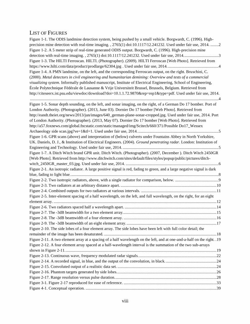
The system, depicted in Figure 1-1 below being pushed by a vehicle, is touted for its “low
weight” of 50 kg, which is about 110 lb. The system is, “usually… pushed in front of a vehicle,”
likely because of the weight of the system. The system images a swath one meter wide, and
generates images in real time.
Figure 1-1. The ODIS landmine detection system, being pushed by a small vehicle. Borgwardt, C. (1996). High-
precision mine detection with real-time imaging. , 2765(1) doi:10.1117/12.241232. Used under fair use, 2014.
3
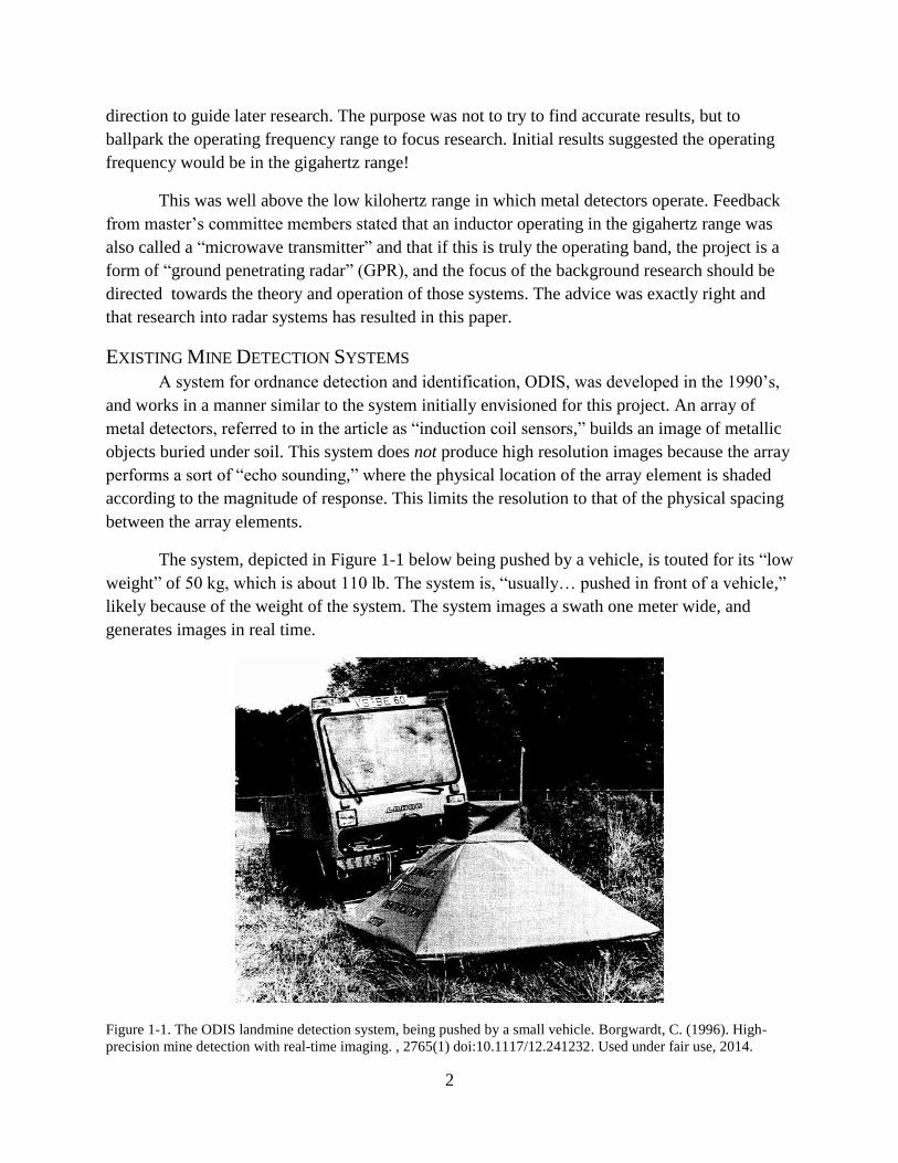
The output of the ODIS, seen in Figure 1-2 below, works okay, but the images are not
crisp enough to be able to differentiate between debris and minimum metal landmines. The
images in Figure 1-2 show a 25cm long, (almost 1 ft.), half-inch wide bar, and it appears similar
in size as if two rifle casings were located next to each other. [6]
Figure 1-2. A 5 meter strip of real-time generated ODIS output. Borgwardt, C. (1996). High-precision mine
detection with real-time imaging. , 2765(1) doi:10.1117/12.241232. Used under fair use, 2014.
From the top down, the objects are: an antipersonnel mine (model PPM2); an iron ball 2 cm in diameter, buried
12 cm deep; a rifle cartridge buried 12 cm deep; an iron bar, 1 cm in diameter, 25 cm long, buried 15 cm deep; and
two objects, an iron ball 5 cm in diameter on the left, buried 25 cm deep, and an anti-tank mine on the right, buried
5 cm deep. [6]
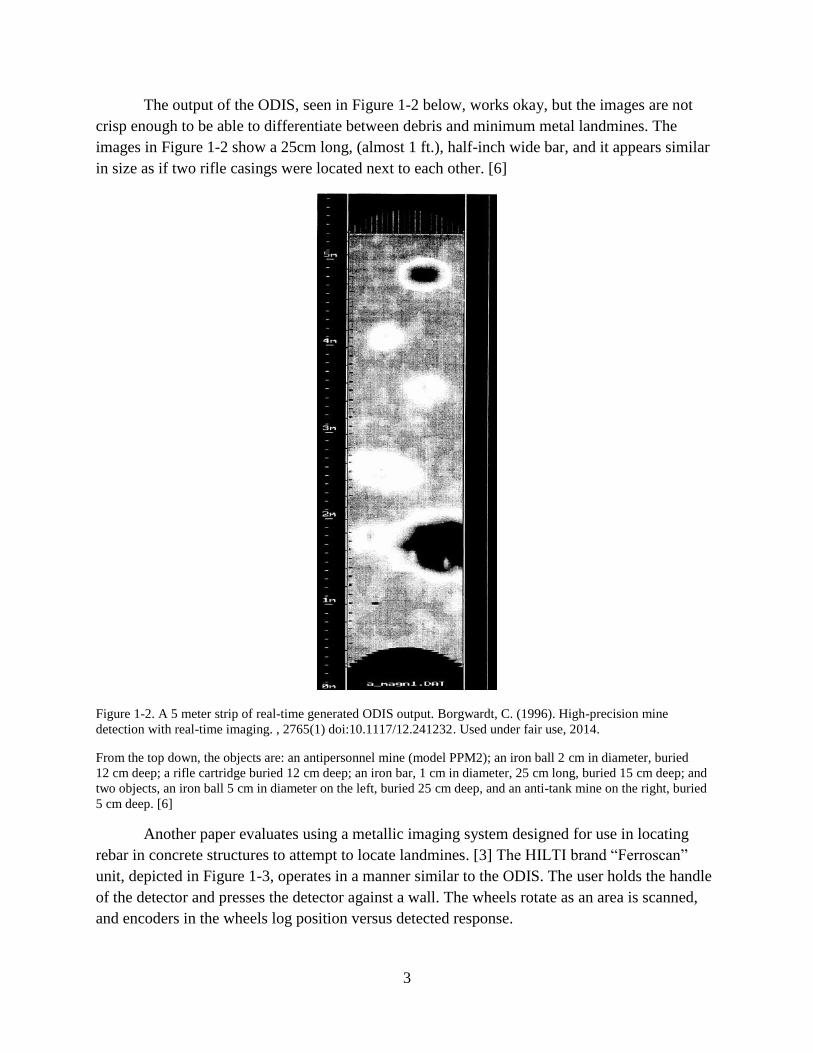
Another paper evaluates using a metallic imaging system designed for use in locating
rebar in concrete structures to attempt to locate landmines. [3] The HILTI brand “Ferroscan”
unit, depicted in Figure 1-3, operates in a manner similar to the ODIS. The user holds the handle
of the detector and presses the detector against a wall. The wheels rotate as an area is scanned,
and encoders in the wheels log position versus detected response.
4
Figure 1-3. The HILTI Ferroscan. HILTI. (Photographer). (2009). HILTI Ferroscan [Web Photo]. Retrieved from
https://www.hilti.com/data/product/prodlarge/62304.jpg . Used under fair use, 2014.
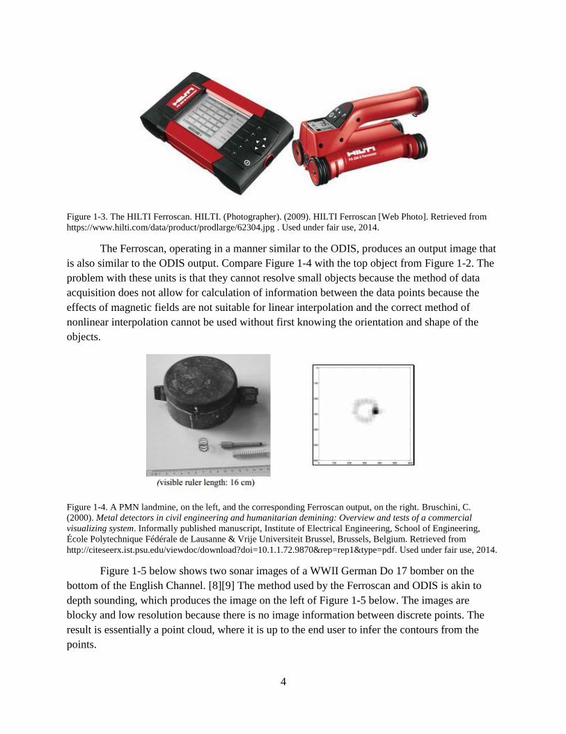
The Ferroscan, operating in a manner similar to the ODIS, produces an output image that
is also similar to the ODIS output. Compare Figure 1-4 with the top object from Figure 1-2. The
problem with these units is that they cannot resolve small objects because the method of data
acquisition does not allow for calculation of information between the data points because the
effects of magnetic fields are not suitable for linear interpolation and the correct method of
nonlinear interpolation cannot be used without first knowing the orientation and shape of the
objects.
Figure 1-4. A PMN landmine, on the left, and the corresponding Ferroscan output, on the right. Bruschini, C.
(2000). Metal detectors in civil engineering and humanitarian demining: Overview and tests of a commercial
visualizing system. Informally published manuscript, Institute of Electrical Engineering, School of Engineering,
École Polytechnique Fédérale de Lausanne & Vrije Universiteit Brussel, Brussels, Belgium. Retrieved from
http://citeseerx.ist.psu.edu/viewdoc/download?doi=10.1.1.72.9870&rep=rep1&type=pdf. Used under fair use, 2014.
Figure 1-5 below shows two sonar images of a WWII German Do 17 bomber on the
bottom of the English Channel. [8][9] The method used by the Ferroscan and ODIS is akin to
depth sounding, which produces the image on the left of Figure 1-5 below. The images are
blocky and low resolution because there is no image information between discrete points. The
result is essentially a point cloud, where it is up to the end user to infer the contours from the
points.

5
Figure 1-5. Sonar depth sounding, on the left, and sonar imaging, on the right, of a German Do 17 bomber. Port of
London Authority. (Photographer). (2013, June 03). Dornier Do 17 bomber [Web Photo]. Retrieved from
http://eandt.theiet.org/news/2013/jun/images/640_german-plane-sonar-cropped.jpg. Used under fair use, 2014. Port
of London Authority. (Photographer). (2013, May 07). Dornier Do 17 bomber [Web Photo]. Retrieved from
http://a57.foxnews.com/global.fncstatic.com/static/managed/img/Scitech/660/371/Possible Do17_Wessex
Archaeology side scan.jpg?ve=1&tl=1. Used under fair use, 2014.
A true imaging system uses an array and post-processing to generate a smoother, more
detailed image, such as the image on the right in Figure 1-5. [9] As mentioned earlier, the
research was guided to ground penetrating radar systems, but the GPR systems researched
produced worse images than the Ferroscan or ODIS! Figure 1-6 below shows real GPR data and
an interpretation of the scan.
Figure 1-6. GPR scans (above) and interpretation of (below) culverts under Fountains Abbey in North Yorkshire,
UK. Daniels, D. J., & Institution of Electrical Engineers. (2004). Ground penetrating radar. London: Institution of
Engineering and Technology. Used under fair use, 2014.
6
The data is hard to understand because the images are typically rendered as two
dimensional (2D) “slices” of the terrain under the GPR unit. This, in turn, is because GPR units
are typically only equipped with one antenna! The relatively low frequencies, in the range of
100MHz to 1GHz, require antennas so large that it is not practical to have a system that uses
multiple antennas. [11][12]
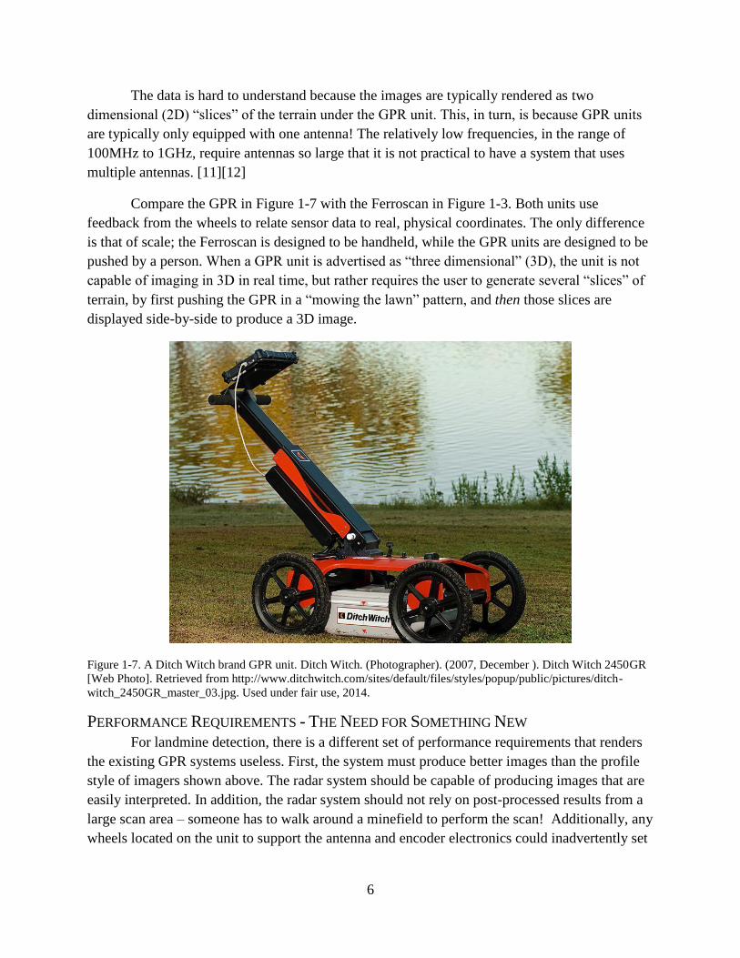
Compare the GPR in Figure 1-7 with the Ferroscan in Figure 1-3. Both units use
feedback from the wheels to relate sensor data to real, physical coordinates. The only difference
is that of scale; the Ferroscan is designed to be handheld, while the GPR units are designed to be
pushed by a person. When a GPR unit is advertised as “three dimensional” (3D), the unit is not
capable of imaging in 3D in real time, but rather requires the user to generate several “slices” of
terrain, by first pushing the GPR in a “mowing the lawn” pattern, and then those slices are
displayed side-by-side to produce a 3D image.
Figure 1-7. A Ditch Witch brand GPR unit. Ditch Witch. (Photographer). (2007, December ). Ditch Witch 2450GR
[Web Photo]. Retrieved from http://www.ditchwitch.com/sites/default/files/styles/popup/public/pictures/ditch-
witch_2450GR_master_03.jpg. Used under fair use, 2014.
PERFORMANCE REQUIREMENTS - THE NEED FOR SOMETHING NEW
For landmine detection, there is a different set of performance requirements that renders
the existing GPR systems useless. First, the system must produce better images than the profile
style of imagers shown above. The radar system should be capable of producing images that are
easily interpreted. In addition, the radar system should not rely on post-processed results from a
large scan area – someone has to walk around a minefield to perform the scan! Additionally, any
wheels located on the unit to support the antenna and encoder electronics could inadvertently set
7
off a landmine. The images should be rendered in real time, and the images should be rendered
in a three dimensional (3D) format that lends itself to quick interpretation.
There are practical limitations on range as well. Landmines are found under shallow
cover, such that the force of a person above is not dispersed by a large layer of soil, so there is no
need to image great distances into the ground, as with surveying equipment. Additionally, unlike
surveying equipment, which is expected to locate large underground features, the landmine
detector should have a resolution high enough to be able to distinguish between shrapnel, bullets,
and the firing pin in a landmine.
A high resolution, low range, handheld, 3D, real-time imaging radar system does not
exist. The remainder of this paper describes the technical specifications and signal processing
requirements necessary to produce such a device. Chapter 2 describes the concepts behind how
an imaging radar system works. It is firmly believed that a conceptual understanding is required
in order to make sense of the radar equations shown in Chapter 3.
With a firm understanding of the concepts, the usage of the governing equations becomes
very straightforward, and, given the required performance specifications, the full system details
are derived relatively quickly. Chapter 4 describes the physical constraints that drive the system
design and explain the choice of targets, and Chapter 5 discusses the results of the MATLAB
simulations under a variety of scenarios. Lastly, Chapter 6 discusses limitations of the system
simulations and makes note of practical physical limitations that were not considered as part of
the system design.
8
Chapter 2 RADAR MECHANICS CONCEPTUAL DESCRIPTION
CHAPTER SUMMARY
This chapter explains how an imaging radar system actually works. Discrete and
continuous apertures are built up from isotropic radiators, and the relationship between aperture
size, operating frequency, and beamwidth is discussed. The mechanics of beam steering are
explained, along with reciprocity and the relationship between transmitters and receivers.
Finally, this chapter discusses the tradeoff between continuous and pulsed radar systems, and
discusses the signal processing needs for the pulsed radar system designed in this paper.
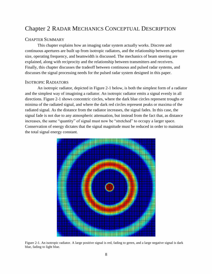
ISOTROPIC RADIATORS
An isotropic radiator, depicted in Figure 2-1 below, is both the simplest form of a radiator
and the simplest way of imagining a radiator. An isotropic radiator emits a signal evenly in all
directions. Figure 2-1 shows concentric circles, where the dark blue circles represent troughs or
minima of the radiated signal, and where the dark red circles represent peaks or maxima of the
radiated signal. As the distance from the radiator increases, the signal fades. In this case, the
signal fade is not due to any atmospheric attenuation, but instead from the fact that, as distance
increases, the same “quantity” of signal must now be “stretched” to occupy a larger space.
Conservation of energy dictates that the signal magnitude must be reduced in order to maintain
the total signal energy constant.
Figure 2-1. An isotropic radiator. A large positive signal is red, fading to green, and a large negative signal is dark
blue, fading to light blue.
9
The isotropic radiator shown appears two dimensional, but a true isotropic radiator emits
the signal evenly in all directions. That is, the isotropic radiator is actually a stack of concentric
spheres instead of circles, like an onion, and the view in Figure 2-1 is similar to an onion sliced
in half, looking at the sliced surface.
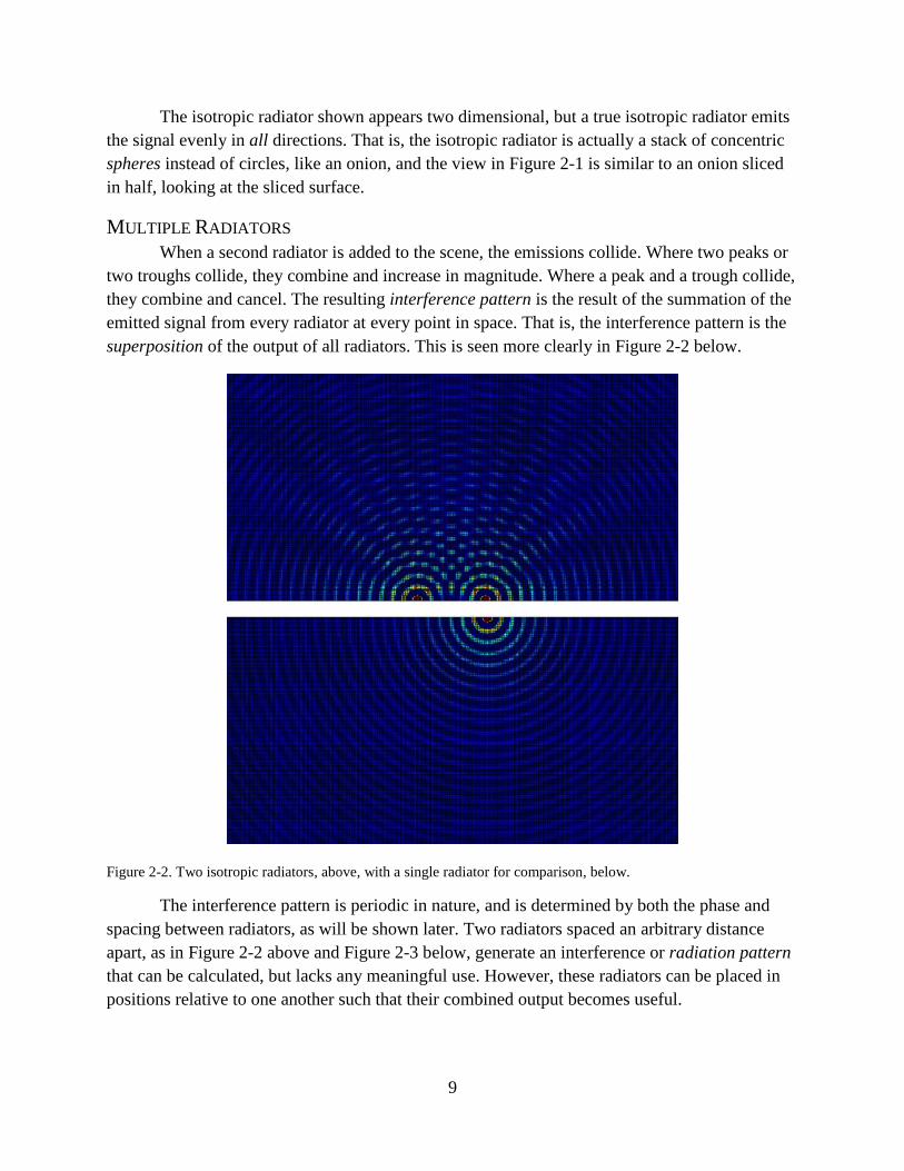
MULTIPLE RADIATORS
When a second radiator is added to the scene, the emissions collide. Where two peaks or
two troughs collide, they combine and increase in magnitude. Where a peak and a trough collide,
they combine and cancel. The resulting interference pattern is the result of the summation of the
emitted signal from every radiator at every point in space. That is, the interference pattern is the
superposition of the output of all radiators. This is seen more clearly in Figure 2-2 below.
Figure 2-2. Two isotropic radiators, above, with a single radiator for comparison, below.
The interference pattern is periodic in nature, and is determined by both the phase and
spacing between radiators, as will be shown later. Two radiators spaced an arbitrary distance
apart, as in Figure 2-2 above and Figure 2-3 below, generate an interference or radiation pattern
that can be calculated, but lacks any meaningful use. However, these radiators can be placed in
positions relative to one another such that their combined output becomes useful.
10
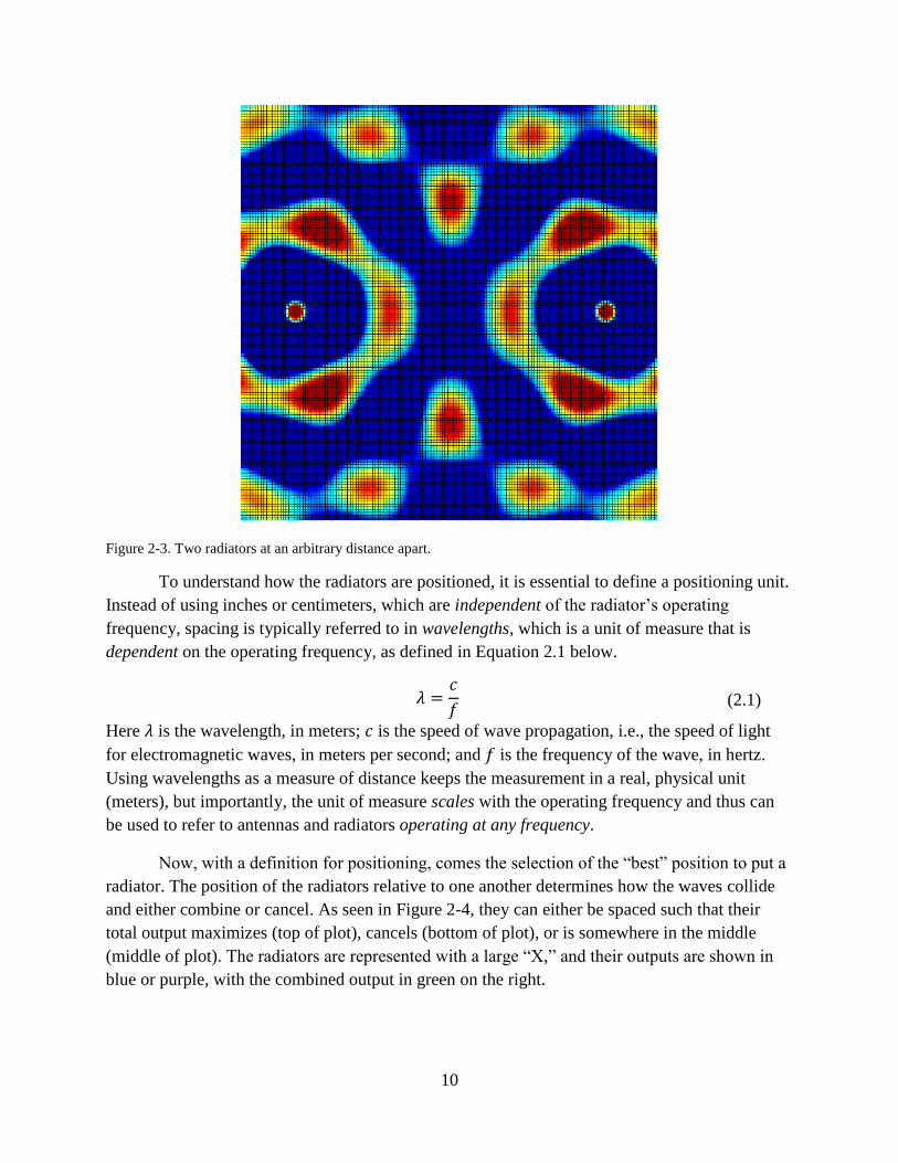
Figure 2-3. Two radiators at an arbitrary distance apart.
To understand how the radiators are positioned, it is essential to define a positioning unit.
Instead of using inches or centimeters, which are independent of the radiator’s operating
frequency, spacing is typically referred to in wavelengths, which is a unit of measure that is
dependent on the operating frequency, as defined in Equation 2.1 below.
(2.1)
Here is the wavelength, in meters; is the speed of wave propagation, i.e., the speed of light
for electromagnetic waves, in meters per second; and is the frequency of the wave, in hertz.
Using wavelengths as a measure of distance keeps the measurement in a real, physical unit
(meters), but importantly, the unit of measure scales with the operating frequency and thus can
be used to refer to antennas and radiators operating at any frequency.
Now, with a definition for positioning, comes the selection of the “best” position to put a
radiator. The position of the radiators relative to one another determines how the waves collide
and either combine or cancel. As seen in Figure 2-4, they can either be spaced such that their
total output maximizes (top of plot), cancels (bottom of plot), or is somewhere in the middle
(middle of plot). The radiators are represented with a large “X,” and their outputs are shown in
blue or purple, with the combined output in green on the right.
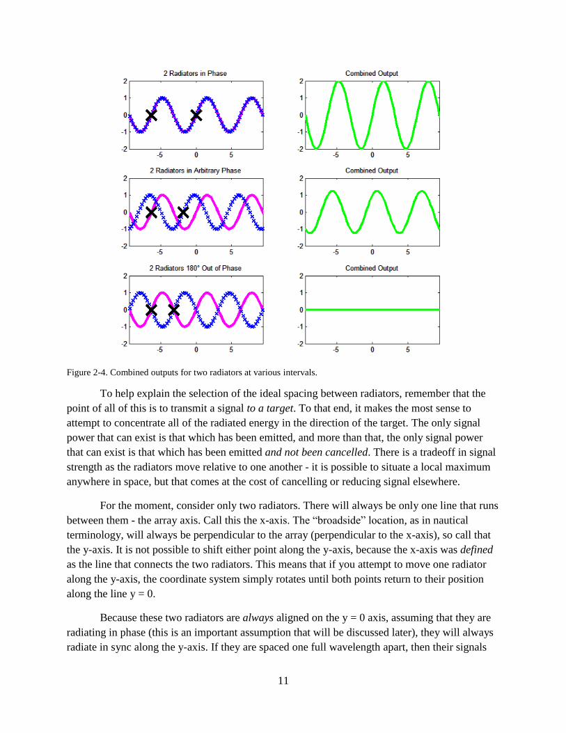
11
Figure 2-4. Combined outputs for two radiators at various intervals.
To help explain the selection of the ideal spacing between radiators, remember that the
point of all of this is to transmit a signal to a target. To that end, it makes the most sense to
attempt to concentrate all of the radiated energy in the direction of the target. The only signal
power that can exist is that which has been emitted, and more than that, the only signal power
that can exist is that which has been emitted and not been cancelled. There is a tradeoff in signal
strength as the radiators move relative to one another - it is possible to situate a local maximum
anywhere in space, but that comes at the cost of cancelling or reducing signal elsewhere.
For the moment, consider only two radiators. There will always be only one line that runs
between them - the array axis. Call this the x-axis. The “broadside” location, as in nautical
terminology, will always be perpendicular to the array (perpendicular to the x-axis), so call that
the y-axis. It is not possible to shift either point along the y-axis, because the x-axis was defined
as the line that connects the two radiators. This means that if you attempt to move one radiator
along the y-axis, the coordinate system simply rotates until both points return to their position
along the line y = 0.
Because these two radiators are always aligned on the y = 0 axis, assuming that they are
radiating in phase (this is an important assumption that will be discussed later), they will always
radiate in sync along the y-axis. If they are spaced one full wavelength apart, then their signals
12
will exactly overlap and they will also radiate in sync along the x-axis. But, because they have
been aligned to purposefully maximize along two axes, they are dividing their total radiative
power along two axes.
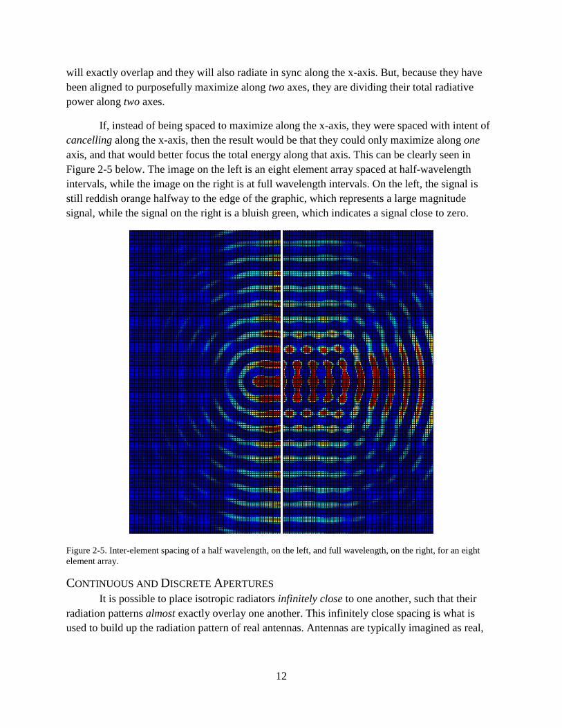
If, instead of being spaced to maximize along the x-axis, they were spaced with intent of
cancelling along the x-axis, then the result would be that they could only maximize along one
axis, and that would better focus the total energy along that axis. This can be clearly seen in
Figure 2-5 below. The image on the left is an eight element array spaced at half-wavelength
intervals, while the image on the right is at full wavelength intervals. On the left, the signal is
still reddish orange halfway to the edge of the graphic, which represents a large magnitude
signal, while the signal on the right is a bluish green, which indicates a signal close to zero.
Figure 2-5. Inter-element spacing of a half wavelength, on the left, and full wavelength, on the right, for an eight
element array.
CONTINUOUS AND DISCRETE APERTURES
It is possible to place isotropic radiators infinitely close to one another, such that their
radiation patterns almost exactly overlay one another. This infinitely close spacing is what is
used to build up the radiation pattern of real antennas. Antennas are typically imagined as real,
13
physical devices, through which a signal is transmitted or received. While this is true, it is also
possible to send or receive a signal from an imaginary surface that is not a physical antenna.
Photographers are used to the term aperture in reference to the opening in a camera
through which light can enter. The light that exposes an image is not created by the aperture, but
nonetheless it diverges from the aperture as though it was. Another, easier, example to imagine is
a mirror. It is possible to direct light from a flashlight or other source with a mirror. The mirror is
not creating the light, but it doesn’t matter! The light still shines from the mirror as if it had
created the light.
Therein lies the difference between an antenna and an aperture. The word “antenna”
refers to the device that generates or ultimately receives the signal, while the word “aperture”
refers to the surface from which a signal is transmitted or received. For most devices, antenna
and aperture are synonymous, but there are a great many examples where they are not.
For instance, your voice is not created in your mouth; it is generated by your vocal cords,
in your throat. Your voice does not come from your throat though, nor does it come from your
tongue or your teeth. Your voice leaves your body through the imaginary surface that exists
between your lips! When you cup your hands to your mouth to be heard at greater distances, you
are not focusing your voice with your hands, you are increasing the effective size of that
imaginary surface between your lips. The focusing is done not by your palms, but by the opening
at the edges of your hands. You are literally giving yourself a bigger mouth (a larger aperture).
Surfaces like your mouth, a car antenna, a mirror, and others are referred to as continuous
apertures because they are one continuous body. This is the most common case, but apertures
can also be sampled or discrete. To imagine a discretized aperture, compare a string of holiday
lights wrapped around a stick to a long fluorescent light bulb. Both are about the same size,
about the same length, and both may illuminate a room about the same. The fluorescent bulb has
a continuous surface that emits light, while the holiday lights are discrete bulbs whose sum
approximates the continuous light-emitting surface of the fluorescent bulb.
A discrete aperture made of elements arranged on a regular spacing can be referred to as
an array, and how well an array approximates a continuous aperture depends on the number of
elements involved and the spacing between those elements. As discussed earlier, for this
purpose, the “best” inter-element spacing is every half wavelength. If the inter-element spacing
is fixed and the desired aperture width is known, then the number of elements required can be
quickly determined. The importance of the aperture size is discussed next.
BEAMWIDTH
The resolution delivered by the imaging system is ultimately determined by the width of
the beam used by the system. Consider television or picture resolution ratings. Typically
measured in “pixels” or “megapixels,” a higher pixel count means a higher resolution image,
which in turn means a sharper, more detailed image. A standard definition television signal is
14
480 pixels across, a high resolution broadcast signals is 720 pixels across, and an ultra-high
resolution signal, such as that found on a Blu-Ray disc, is 1080 pixels across.
The higher pixel count means that there are more data points in a given image with which
to reproduce the initial scene. If the television or picture’s physical dimensions remain constant,
then a higher resolution image requires the individual pixels to be physically smaller than those
of the lower resolution image. The actual dimensions of the pixels are measured with Cartesian
coordinates because the pixels exist on a planar surface.
With radar systems, the image resolution is determined by the beamwidth and by the size
of the increment used to “steer” the beam to a given location. The mechanics of beam steering
will be discussed shortly, but suffice it to say that the output of the radar array can be pointed in
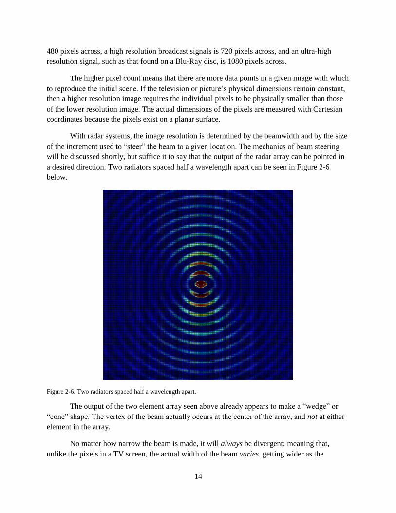
a desired direction. Two radiators spaced half a wavelength apart can be seen in Figure 2-6
below.
Figure 2-6. Two radiators spaced half a wavelength apart.
The output of the two element array seen above already appears to make a “wedge” or
“cone” shape. The vertex of the beam actually occurs at the center of the array, and not at either
element in the array.
No matter how narrow the beam is made, it will always be divergent; meaning that,
unlike the pixels in a TV screen, the actual width of the beam varies, getting wider as the
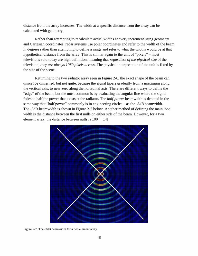
15
distance from the array increases. The width at a specific distance from the array can be
calculated with geometry.
Rather than attempting to recalculate actual widths at every increment using geometry
and Cartesian coordinates, radar systems use polar coordinates and refer to the width of the beam
in degrees rather than attempting to define a range and refer to what the widths would be at that
hypothetical distance from the array. This is similar again to the unit of “pixels” – most
televisions sold today are high definition, meaning that regardless of the physical size of the
television, they are always 1080 pixels across. The physical interpretation of the unit is fixed by
the size of the scene.
Returning to the two radiator array seen in Figure 2-6, the exact shape of the beam can
almost be discerned, but not quite, because the signal tapers gradually from a maximum along
the vertical axis, to near zero along the horizontal axis. There are different ways to define the
“edge” of the beam, but the most common is by evaluating the angular line where the signal
fades to half the power that exists at the radiator. The half-power beamwidth is denoted in the
same way that “half power” commonly is in engineering circles – as the -3dB beamwidth.
The -3dB beamwidth is shown in Figure 2-7 below. Another method of defining the main lobe
width is the distance between the first nulls on either side of the beam. However, for a two
element array, the distance between nulls is 180°! [14]
Figure 2-7. The -3dB beamwidth for a two element array.
16
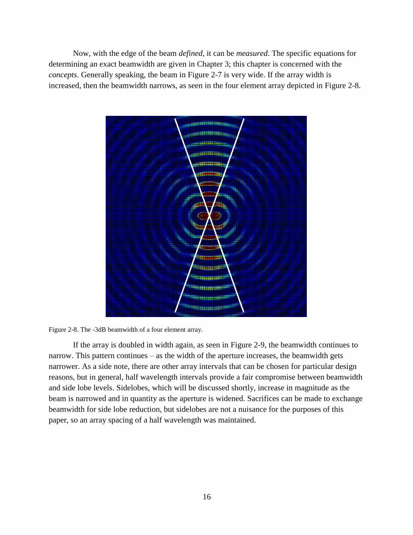
Now, with the edge of the beam defined, it can be measured. The specific equations for
determining an exact beamwidth are given in Chapter 3; this chapter is concerned with the
concepts. Generally speaking, the beam in Figure 2-7 is very wide. If the array width is
increased, then the beamwidth narrows, as seen in the four element array depicted in Figure 2-8.
Figure 2-8. The -3dB beamwidth of a four element array.
If the array is doubled in width again, as seen in Figure 2-9, the beamwidth continues to
narrow. This pattern continues – as the width of the aperture increases, the beamwidth gets
narrower. As a side note, there are other array intervals that can be chosen for particular design
reasons, but in general, half wavelength intervals provide a fair compromise between beamwidth
and side lobe levels. Sidelobes, which will be discussed shortly, increase in magnitude as the
beam is narrowed and in quantity as the aperture is widened. Sacrifices can be made to exchange
beamwidth for side lobe reduction, but sidelobes are not a nuisance for the purposes of this
paper, so an array spacing of a half wavelength was maintained.
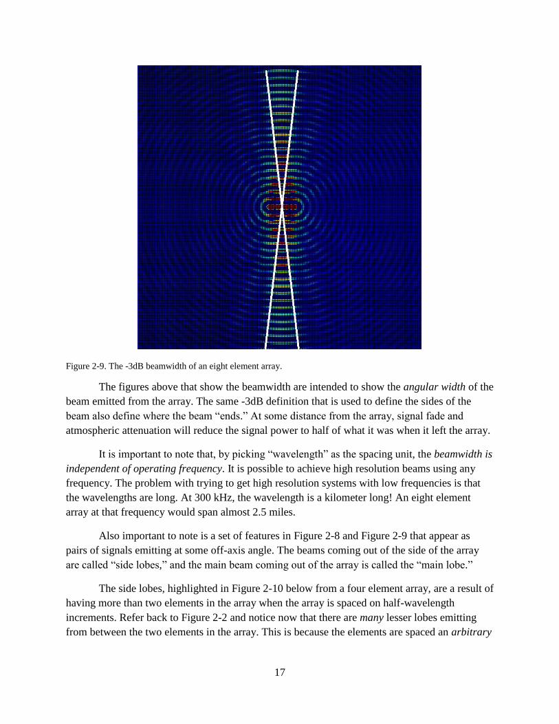
17
Figure 2-9. The -3dB beamwidth of an eight element array.
The figures above that show the beamwidth are intended to show the angular width of the
beam emitted from the array. The same -3dB definition that is used to define the sides of the
beam also define where the beam “ends.” At some distance from the array, signal fade and
atmospheric attenuation will reduce the signal power to half of what it was when it left the array.
It is important to note that, by picking “wavelength” as the spacing unit, the beamwidth is
independent of operating frequency. It is possible to achieve high resolution beams using any
frequency. The problem with trying to get high resolution systems with low frequencies is that
the wavelengths are long. At 300 kHz, the wavelength is a kilometer long! An eight element
array at that frequency would span almost 2.5 miles.
Also important to note is a set of features in Figure 2-8 and Figure 2-9 that appear as
pairs of signals emitting at some off-axis angle. The beams coming out of the side of the array
are called “side lobes,” and the main beam coming out of the array is called the “main lobe.”
The side lobes, highlighted in Figure 2-10 below from a four element array, are a result of
having more than two elements in the array when the array is spaced on half-wavelength
increments. Refer back to Figure 2-2 and notice now that there are many lesser lobes emitting
from between the two elements in the array. This is because the elements are spaced an arbitrary
18
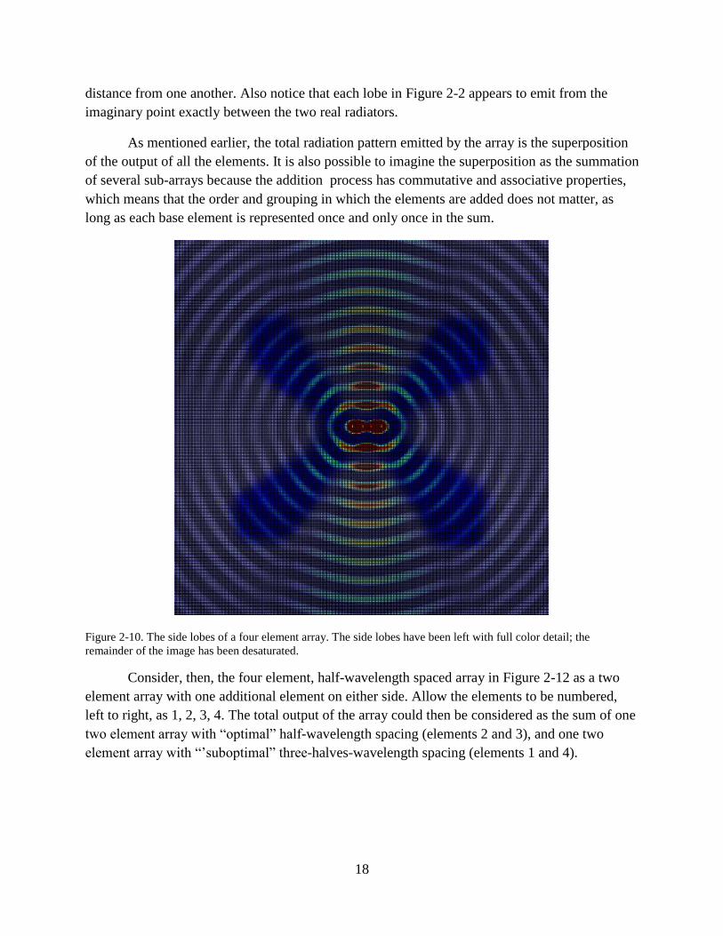
distance from one another. Also notice that each lobe in Figure 2-2 appears to emit from the
imaginary point exactly between the two real radiators.
As mentioned earlier, the total radiation pattern emitted by the array is the superposition
of the output of all the elements. It is also possible to imagine the superposition as the summation
of several sub-arrays because the addition process has commutative and associative properties,
which means that the order and grouping in which the elements are added does not matter, as
long as each base element is represented once and only once in the sum.
Figure 2-10. The side lobes of a four element array. The side lobes have been left with full color detail; the
remainder of the image has been desaturated.
Consider, then, the four element, half-wavelength spaced array in Figure 2-12 as a two
element array with one additional element on either side. Allow the elements to be numbered,
left to right, as 1, 2, 3, 4. The total output of the array could then be considered as the sum of one
two element array with “optimal” half-wavelength spacing (elements 2 and 3), and one two
element array with “’suboptimal” three-halves-wavelength spacing (elements 1 and 4).
19
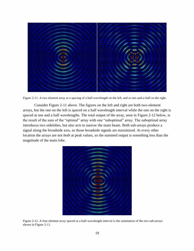
Figure 2-11. A two element array at a spacing of a half wavelength on the left, and at one-and-a-half on the right.
Consider Figure 2-11 above. The figures on the left and right are both two-element
arrays, but the one on the left is spaced on a half wavelength interval while the one on the right is
spaced at one and a half wavelengths. The total output of the array, seen in Figure 2-12 below, is
the result of the sum of the “optimal” array with one “suboptimal” array. The suboptimal array
introduces two sidelobes, but also acts to narrow the main beam. Both sub-arrays produce a
signal along the broadside axis, so those broadside signals are maximized. At every other
location the arrays are not both at peak values, so the summed output is something less than the
magnitude of the main lobe.
Figure 2-12. A four element array spaced at a half-wavelength interval is the summation of the two sub-arrays
shown in Figure 2-11.
20
BEAM STEERING
The “optimal” array spacing was determined by evaluating the output of two antennas
that are radiating in phase with one another. This assumption was made earlier, in the Multiple
Radiators section, with the promise that it would be discussed later. The effects of out-of-phase
radiators are discussed now.
The half-wavelength spacing between elements served two purposes. First, it ensured that
the signal was canceled along the array axis, and second, by canceling along the array axis, the
broadside signal was maximized. The decision to cancel along the array axis was made because
there was no way to cancel along the broadside direction, because the signals could not be
shifted relative to one another along the broadside axis. However, if a phase difference is
introduced between the radiating elements, then the effect is as if they had been physically
repositioned.
Now, with a phase shift, it is possible to cancel along the broadside axis! Shifting one
radiator half a cycle in phase (180°) corresponds to moving it physically by half a wavelength.
As discussed at length earlier, by effectively “moving” the radiator half a wavelength, the signals
now cancel along the broadside axis. However, the radiator was not physically repositioned, so it
is still located on the array axis, where it remains physically spaced half a wavelength from the
other radiator.
Now, being shifted, one radiator is effectively half a wavelength away from the other
because of the phase shift, and now it’s also half a wavelength away because it’s physically
located half a wavelength away. That is, the radiators exist “as if” they were spaced half a
wavelength apart on the broadside axis, and “as if” they were spaced a full wavelength apart on
the array axis. This means that, while the signals cancel along broadside, they now combine and
maximize along the array axis.
The transition between maximizing along the broadside axis and maximizing along the
array axis is not instantaneous! If the phase difference were to gradually change, the axis of
maximization would slowly move from broadside towards the array axis. If there is no phase
shift, the array output is at broadside. As the phase shift increases towards +180°, the array
output “points” more towards one side. The array becomes an “endfire” array, meaning an array
that emits along the array axis, when the phase shift reaches 180°.
As the phase shift is decreased towards -180°, the beam points towards the other side,
becoming an endfire array along the opposite end when the phase shift reaches -180°. The
particulars of which direction the beam points depend on how you, the designer, define the
coordinate system and how you define a positive or negative phase shift.
21
PULSED VS. CONTINUOUS WAVE RADAR
The two main categories of radar systems, in terms of overall operation, are continuous
wave and pulse. These systems operate exactly the way they sound – continuous wave systems
have transmitters that are always on, while pulsed systems turn on the transmitters for a short
period of time, then turn them off and “listen” for an echo.
Conceptually speaking, pulsed systems are the most straightforward to understand.
Transmit a brief signal, and then count the time that elapses until an echo is received. The
distance between the array and the target is the elapsed time multiplied by the speed of wave
propagation, e.g., the speed of light for radar, or the speed of sound for sonar. The transmitter is
turned off whenever the receiver is turned on, so the receiver has a “quiet” environment in which
to listen for a response.
Continuous wave radar, without any form of signal modulation, cannot determine
distance because the output is continuous. There is no reference point defining the “start” of the
signal, so it is not possible to determine the time between transmission and reception. Without an
elapsed time, it is not possible to calculate range.
The solution to creating a time reference with continuous wave radar is to modulate the
signal such that there is a definite way with which to correlate a response to a known point in
time. Frequency modulation provides the means to transform a continuous fixed frequency
output to a range of frequencies. The length of time to cycle through the range of frequencies is
not fixed, but it is usually a “long” time period. Here “long” means that the time that should
elapse before revisiting the first frequency should be at least as long or longer than the time that
it would take to receive a signal from the maximum range of the unit.
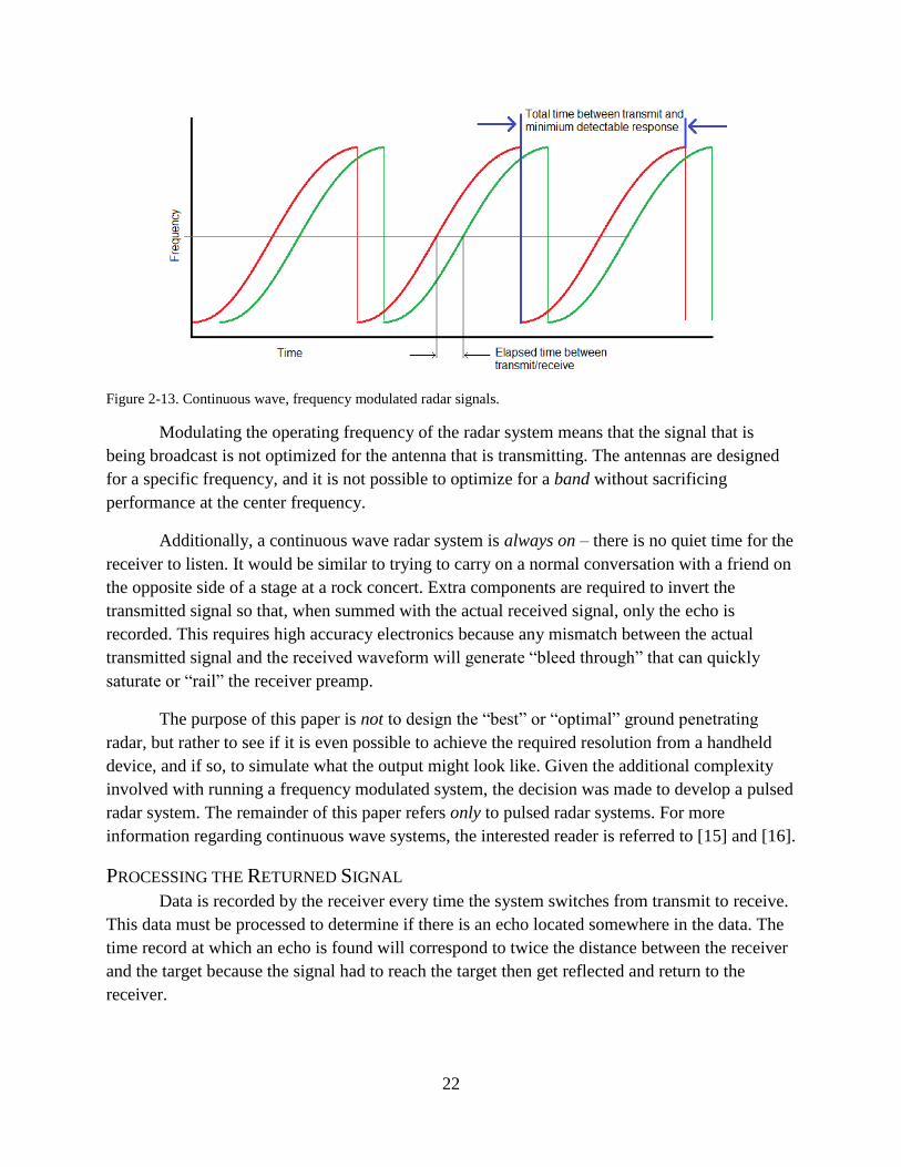
Consider Figure 2-13 below. The frequency modulation method is similar to a chirp
signal, where the signal starts at some relatively low frequency then rises to a higher frequency
before repeating the signal. If the signal repeats before a response from the maximum range
could be received, then it would not be possible for the system to differentiate between a very
close and a very far target. A long modulation period ensures ranging accuracy.
22
Figure 2-13. Continuous wave, frequency modulated radar signals.
Modulating the operating frequency of the radar system means that the signal that is
being broadcast is not optimized for the antenna that is transmitting. The antennas are designed
for a specific frequency, and it is not possible to optimize for a band without sacrificing
performance at the center frequency.
Additionally, a continuous wave radar system is always on – there is no quiet time for the
receiver to listen. It would be similar to trying to carry on a normal conversation with a friend on
the opposite side of a stage at a rock concert. Extra components are required to invert the
transmitted signal so that, when summed with the actual received signal, only the echo is
recorded. This requires high accuracy electronics because any mismatch between the actual
transmitted signal and the received waveform will generate “bleed through” that can quickly
saturate or “rail” the receiver preamp.
The purpose of this paper is not to design the “best” or “optimal” ground penetrating
radar, but rather to see if it is even possible to achieve the required resolution from a handheld
device, and if so, to simulate what the output might look like. Given the additional complexity
involved with running a frequency modulated system, the decision was made to develop a pulsed
radar system. The remainder of this paper refers only to pulsed radar systems. For more
information regarding continuous wave systems, the interested reader is referred to [15] and [16].
PROCESSING THE RETURNED SIGNAL
Data is recorded by the receiver every time the system switches from transmit to receive.
This data must be processed to determine if there is an echo located somewhere in the data. The
time record at which an echo is found will correspond to twice the distance between the receiver
and the target because the signal had to reach the target then get reflected and return to the
receiver.
23
The signal processing required is generally straightforward, but there are some finer
points that may not be immediately obvious that will also be mentioned. Consider first a pulse
that is transmitted, reflected, received, and recorded, with no noise or attenuation. At first, it may
seem trivial to determine when the pulse was received – just look for the peak!
However, remember that the pulse is a high frequency signal, and that there are many
peaks in a sinusoid. Figuring out which peak represents the moment the signal is received can
actually be very challenging. The best way to determine the exact response is to compare what
the receiver recorded with what you know you sent. You are the system designer! You can utilize
this a priori knowledge of the transmitted signal to “look” specifically for that waveform.
The waveform that is received isn’t going to be exactly the waveform that was
transmitted, though. Remember that the wave reaches the receiver only after being reflected. The
reflection inverts the wave. Looking into a mirror, your left side becomes your image’s right
side. Similarly, the start of the wave, which was the first to leave the transmitter, is the first to get
reflected, and the first to enter the receiver. The end of the wave becomes the newest or most
recent entry in the receiver data log.
Mathematically, an operation that mirrors a signal and then filters a long data record
looking for the mirrored signal is called a convolution. The convolution process overlays one
waveform (called the “window”) over another waveform (the record), and multiplies the two at
every time record at which the two overlap. All of the products are then summed to produce one
sample at the appropriate “lag” or waveform offset.
The action of multiplying then summing produces an effect that is not immediately
apparent. Anywhere the window is positive and the record is negative, or vice versa, the product
is negative. This represents regions where the signals do not match. Only when the window and
record are the same sign, negative-negative or positive-positive, will the resulting product be
positive. This represents regions where the window and record do match.
This pattern, where the output at each point is positive for a match and negative for no
match, is repeated for every point in the window, and the output then gets summed. If there is a
random signal, then there is an expectation that the window would randomly match or not match.
When summed, the output is expected to be the mean for the random signal, typically zero. Only
when the window “mostly” matches with the data will a positive record be produced, and the
maximum output of the convolution corresponds to where the window most matches the record.
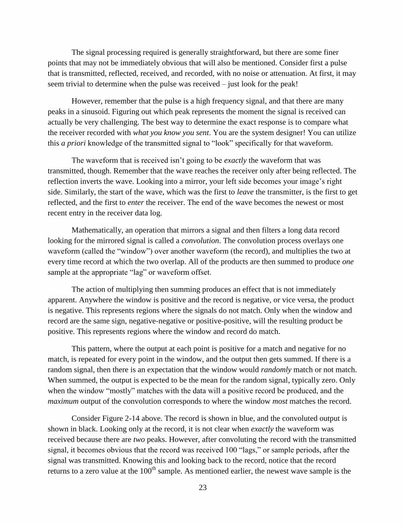
Consider Figure 2-14 above. The record is shown in blue, and the convoluted output is
shown in black. Looking only at the record, it is not clear when exactly the waveform was
received because there are two peaks. However, after convoluting the record with the transmitted
signal, it becomes obvious that the record was received 100 “lags,” or sample periods, after the
signal was transmitted. Knowing this and looking back to the record, notice that the record
returns to a zero value at the 100th
sample. As mentioned earlier, the newest wave sample is the
24
last one to leave the transmitter. That means that the waveform in blue left the transmitter 100
sample periods ago.
Figure 2-14. A recorded signal, in blue, and the output of the convolution, in black.
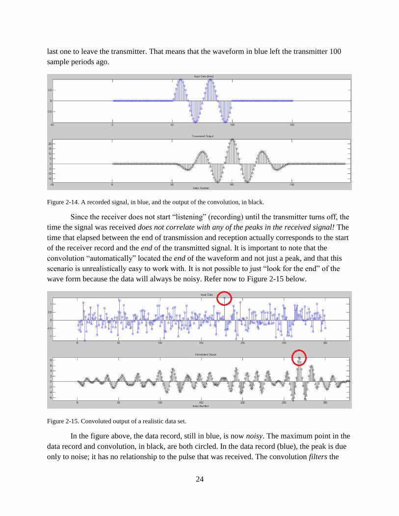
Since the receiver does not start “listening” (recording) until the transmitter turns off, the
time the signal was received does not correlate with any of the peaks in the received signal! The
time that elapsed between the end of transmission and reception actually corresponds to the start
of the receiver record and the end of the transmitted signal. It is important to note that the
convolution “automatically” located the end of the waveform and not just a peak, and that this
scenario is unrealistically easy to work with. It is not possible to just “look for the end” of the
wave form because the data will always be noisy. Refer now to Figure 2-15 below.
Figure 2-15. Convoluted output of a realistic data set.
In the figure above, the data record, still in blue, is now noisy. The maximum point in the
data record and convolution, in black, are both circled. In the data record (blue), the peak is due
only to noise; it has no relationship to the pulse that was received. The convolution filters the
25
data, using the known waveform, and discovers the actual received signal time at approximately
270 sample periods.
The use of a convolution to filter data to find a matching signal is referred to as matched
filtering. This technique improves the detectability of a signal in a noisy data set; that is, it
improves the signal-to-noise ratio (SNR) of the receiver.
It is also possible to improve the signal to noise ratio by re-sampling. Assuming the noise
is zero-mean, Gaussian distributed noise, a pulse could be sent several times, and the resulting
series of pulses could be averaged or integrated. The random, normally distributed noise should
approach the expected value (its mean, i.e., zero) as the number of pulses increases. This has the
advantage of reducing the total broadcast power required to achieve a desired SNR, but comes at
the cost of requiring a longer amount of time at each “look” angle.
SIDELOBES AND PHANTOM IMAGES
The last signal processing step is to determine which peak constitutes a “valid” echo.
Refer again to Figure 2-15, and notice that, on the black “filtered” output, the circled peak is the
highest peak, but it is not the only peak.
A threshold could be established, above which a signal could be deemed valid, but the
issue with setting a fixed threshold is that the signal fades as distance increases. Compounding
this problem are the side lobes. They were mentioned briefly earlier, and highlighted in Figure
2-10. The sidelobes are a real transmission of the array, at some angle other than the expected
output angle of the array.
Consider an array that, as in Figure 2-12, has a pair of sidelobes that exist at a ±60° angle
from the main lobe. Now, place the array in a void, with only one other object in existence to
reflect. If the object is located at broadside and the array is not steered, the main lobe illuminates
the target, and the receiver locates the echo of the main lobe and records that it found an object.
Now the main lobe is steered, from 0° towards 60°. No other objects exist, so the receiver does
not record any objects detected.
26
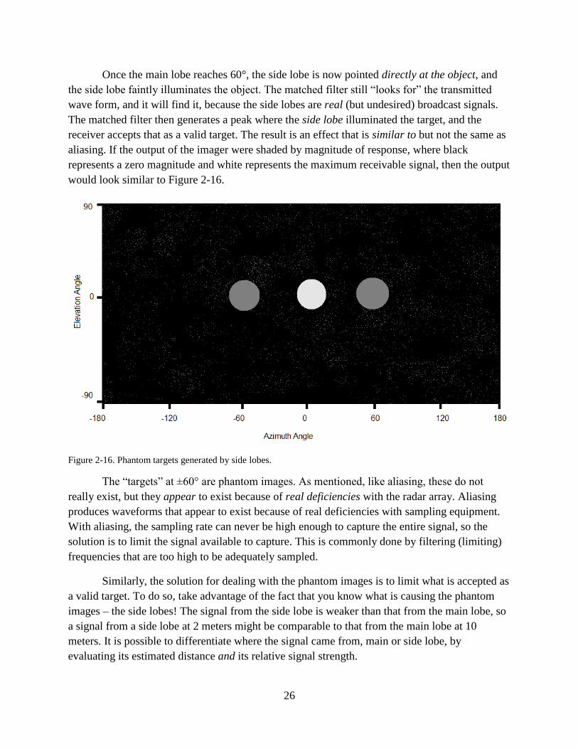
Once the main lobe reaches 60°, the side lobe is now pointed directly at the object, and
the side lobe faintly illuminates the object. The matched filter still “looks for” the transmitted
wave form, and it will find it, because the side lobes are real (but undesired) broadcast signals.
The matched filter then generates a peak where the side lobe illuminated the target, and the
receiver accepts that as a valid target. The result is an effect that is similar to but not the same as
aliasing. If the output of the imager were shaded by magnitude of response, where black
represents a zero magnitude and white represents the maximum receivable signal, then the output
would look similar to Figure 2-16.
Figure 2-16. Phantom targets generated by side lobes.
The “targets” at ±60° are phantom images. As mentioned, like aliasing, these do not
really exist, but they appear to exist because of real deficiencies with the radar array. Aliasing
produces waveforms that appear to exist because of real deficiencies with sampling equipment.
With aliasing, the sampling rate can never be high enough to capture the entire signal, so the
solution is to limit the signal available to capture. This is commonly done by filtering (limiting)
frequencies that are too high to be adequately sampled.
Similarly, the solution for dealing with the phantom images is to limit what is accepted as
a valid target. To do so, take advantage of the fact that you know what is causing the phantom
images – the side lobes! The signal from the side lobe is weaker than that from the main lobe, so
a signal from a side lobe at 2 meters might be comparable to that from the main lobe at 10
meters. It is possible to differentiate where the signal came from, main or side lobe, by
evaluating its estimated distance and its relative signal strength.
27
A weak signal at an estimated distance of 2 meters should be rejected, while the same
signal at an estimated distance of 10 meters should be accepted. The method typically used to
compare signal strengths is a method of normalizing the signals strengths, referred to as applying
a time varying gain.
The gain that should be applied is determined by evaluating the signal loss that would
occur from both fading and atmospheric attenuation. That is, a value is added to the received
signal that would enlarge a main lobe’s signal to the same magnitude as it was when it left the
transmitter. A reflection very close to the receiver would need only a little gain to “restore” it to
full power, while a reflection from very far away would need a significant amount of
amplification to return to full power.
The use of the time varying gain would add only a small signal to the already weak side
lobe emission, such that the “normalized” side lobe signal would be significantly smaller than the
main lobe signal at the same point in time. Indeed, since any main lobe reflection should now
exist at the same magnitude regardless of target distance, a threshold can now be applied to the
filtered, normalized data. Any points exceeding the threshold are classified as “valid,” and any
points below the threshold are ignored.
SPHERICAL VS. CARTESIAN RESOLUTION
The topic of resolution was briefly covered in the Beamwidth section of this chapter. The
resolution of the radar system is a description of how well the system is able to represent the
scene at which it is looking. No matter the look angle, the beam always originates from the
center of the array. The system does not take measurements of the scene along a line, it takes the
measurements along an arc.
The system is steered to a particular angle, and measures in three dimensions along an
arc, which means the logical native coordinate system for a radar (or sonar) system is a spherical
coordinate system. The key difference between a radar system’s spherical coordinates and a
standard physics or mathematics based spherical coordinate system is that radar coordinates use
an elevation angle measured from the X-Y plane, whereas most other coordinate systems
measure an inclination or zenith angle from the +Z axis. All systems use an azimuth angle
measured positive when counter-clockwise from the +X axis.
The difficulty in comparing resolutions comes from a familiarity with Cartesian
coordinates, where a measurement in any one location is the same regardless of location. Polar or
spherical coordinate systems utilize angular measurements and, from similar triangles, a linear
distance between two points will increase linearly as the distance from the vertex of the
coordinate system (commonly denoted “ρ”) to each point increases. Two points 3 inches apart
when ρ = 10 inches will be 6 inches apart when ρ = 20 inches.
In a similar manner, the ability of the radar system to determine the width of an object is
dependent on the distance of that object from the array. The beam width is given as an angular

28
measurement, so the width of the beam at a specific point depends on the distance from the
array. As distance to the array increases, an object of constant size is imaged more poorly
because the linear width of the beam that images it has increased.
If it is desirable to achieve a specific linear beam width, as in cases where there is a
specific target in mind, then the angular beam width should be determined by locating that target
at the maximum operating range of the radar system. As the distance from the object to the array
decreases, the linear width of the beam will as well. This is a conservative way to establish a
beam width requirement because it ensures that the required linear width will always be achieved
or exceeded.
RANGE RESOLUTION
A topic that has not been mentioned until now is range or depth resolution. Previously,
all discussions regarding resolution have been about angular resolution, or the ability of the
radar system to resolve the width of an object. It is also important to evaluate the depth or
thickness of an object. Just as the main lobe can smear the width of discrete objects located inside
the beam, the objects located “on top” of one another (sequentially along the beam axis) can
smear the length of the pulse, resulting in the reflection getting averaged into one point that is
located equidistant from both objects. Refer to Figure 2-17 below.
Figure 2-17. Range resolution versus pulse duration.
Figure 2-17 depicts graphically how an overly long pulse can blur two distinct objects
into one. As the transmitted signal (upper left) strikes the nearer object, the wave reflects. After
some period of time, the wave reflects off of the farther object as well. If the pulse is too long,
the front of the wave reflected by the farther object can wind up riding the end of the wave
reflected by the nearer object.
29
As discussed earlier and depicted in Figure 2-14, the matched filter will attempt to “find”
where the signal best matches up with what was transmitted. In this instance, because the
magnitude of the reflected wave is maximized where the waves from the near and far objects
overlap, the “best” match occurs in the middle of the elongated reflection. The middle of this
reflection corresponds with the point located between the two objects.
BASIC OPERATION RECAP
Different aspects of radar imaging have been explained individually up to this point, as
understanding the different concepts involved is crucial to understanding the system as a whole.
The remainder of this chapter takes a moment to explain how all of these individual parts mesh
together to form the full imaging system.
First, the radar designer chooses an aperture wide enough to achieve a desired beam
width. A wide aperture can be achieved by having one large antenna (see: radio telescopes), or
by having an array of small antennas. The wider the aperture, real or discrete, the narrower the
main beam will be.
Then, once a suitable beam width has been selected, a “raster” or scan of the scene
begins. The beam is pointed to a given direction, and the time delay between transmission and
reception is recorded. In the event that the aperture is one large antenna, the only way to point
the beam is to physically move the entire antenna. There are plenty of time-lapse videos on
YouTube of radio telescopes being steered. In the event that the aperture is an array, the beam
can be steered by physically moving the array, by electronically steering the array with phase
delays as discussed earlier, or a combination of the two.
Finally, the receiver waits for an echo. It is not possible to discern where within the main
lobe the reflector (or target) is located. It is not even possible to discern whether the echo came
from the main lobe or from one of the side lobes! The only thing the radar system “knows” is in
which direction it was pointed (again, physically or electronically), and how long it took to
receive the signal.
Upon receipt of an echo, the portion of the device responsible for producing the image
has to assume that the target was as wide as the beam width at whichever distance it was
detected, because again, there is no way to tell whether the target was as wide as the beam, or if
it was located in the center or edges of the beam. This can cause a smearing effect, which is
discussed very well in Kenneth Rolt’s master’s thesis from MIT [17]. Smearing means that
objects as large as or larger than the beam are rendered relatively accurately, while objects
significantly smaller than the beam’s width are smeared until they are displayed to be that wide.
[17] is highly recommended reading for anyone interested in learning more about the imaging
process. Hopefully this paper gives you your “breakthrough” insight into how all of this works;
Kenneth’s paper (which is actually on synthetic aperture sonar) was where everything “clicked”
for the author.

30
The process repeats: point, transmit, receive, and record a data point at the distance
corresponding to the time delay between transmit/receive. Typically the data point will be given
a value that corresponds to the magnitude above the threshold for a valid target. This relative
magnitude information is used to shade the image that is produced. Every time the array is
pointed in a new direction, that position is combined with the intensity or shading value and a
new “pixel” is created. Once the desired scene has been scanned, the beam is typically pointed
back at the starting position and the scene re-scanned. Due to the high speeds associated with
radar, electronic beam steering can allow the scene to be rescanned dozens to hundreds of times
every second, producing “real time” video quality image refresh rates.
31
Chapter 3 RADAR MECHANICS MATHEMATICAL DESCRIPTION
CHAPTER SUMMARY
Hopefully, having made it this far, you have a firm understanding of how radar arrays are
setup, how the beams are steered, signals are transmitted, and echoes received and processed.
Getting to this point took me months of work! This chapter leverages your understanding of the
concepts to show the formulas that drive the concepts. This chapter, and all the ones that follow,
should be significantly shorter than the last because there isn’t the need to describe why
something is – you already understand how it works!
This chapter does not cover any of the numeric values regarding my proposed radar
imaging system; those are covered in the next chapter, along with my reasoning for choosing
specific values as inputs to the equations given here. The equations shown in this chapter are
discussed in detail, so they may be quickly referenced in the following chapter, with discussion
there about what the results mean instead of where the equation came from.
In reading numerous research papers, experience has shown that deriving every equation
is more tedious for the reader than for the writer. If the derivation is not original, then it is an
exercise in copying and pasting. It is the opinion of the author that lengthy derivations only serve
to “bulk up” a paper while adding little content, and the result is that there is more time for the
reader to get distracted, disinterested, and/or confused. Therefore, the only equations shown are
the ones that are meaningful and intended to be used, or brief derivations to help reinforce the
concepts covered in this paper.
PERFORMANCE METRICS
DETECTION AND THE SIGNAL TO NOISE RATIO
Most of the discussion up to this point has been about ideal systems, with difficulties of
noise being discussed only briefly in the last chapter. In reality, noise is a real concern that
imposes practical limitations on the system. In a noiseless scenario, it would be possible to
infinitely amplify the output of the receiver and have a limitless range on the radar unit.
Random noise creates a “noise floor,” where a small signal and random noise become
indistinguishable from one another. This sets a lower limit (or floor) on the minimum detectable
valid signal, as the returned signal must be greater in magnitude than the noise. The noise is
assumed to be zero-mean and Gaussian in distribution. This means that, for any point in the time
record, the noise could either be positive, boosting a weak (side lobe) signal above the receiver
threshold, or may, very infrequently, be positive and large enough in magnitude such that the
noise could exceed the threshold on its own. Conversely, negatively valued noise could mask a
valid response, preventing it from exceeding the threshold for detection.
32
It is easy to always receive the signal and always reject the noise – just broadcast with
infinite power and set the receiver threshold at infinity! In reality, there is a tradeoff between
broadcast power and the rejection of false positives and negatives. False positives occur when
noise adds to a signal, so the solution is to raise the threshold for detection or reduce the
broadcast power. Similarly, false negatives occur when the threshold is too high or the broadcast
power is too low.
Walter Albersheim derived a formula, now known as the “Albersheim detection
equation,” that approximates a series of receiver operating characteristic (ROC) curves
developed by Bell Labs in 1967 [18]. These ROC curves display, graphically, the tradeoff
between the probabilities of detection and false alarm for a given signal to noise ratio.
Albersheim’s equation, which matches the Bell Labs ROC curves within 0.2dB over almost the
entire range, is given as [19]:
(
√ ) ( ) 3.1
where
(
)
(
)
and M is the number of samples, Pd is the probability of detection, and Pfa is the probability of
false alarm. This equation is derived in [20].
Equation 3.1 above has the term where again, M is the number of samples.
This term is assuming that the multiple samples are used for pulse integration, as described in the
previous chapter. Notice that the term is negative – as more samples are taken, the quantity
becomes more negative, and the required SNR declines.
The decision for the exact values selected for Pfa and Pd are explained in the next chapter,
but the numbers are based on statistical distributions, i.e., a value of “1” means that event will
happen 100% of the time, and a value of “0” means that the event will never happen. Ideally, the
probability of detection would be 1, meaning an object would always be detected, and the
probability of false alarm would be 0, meaning there would never be a false alarm.
Notice that the B term shows that if the probability of detection was in fact 1, the B term
would go to infinity (undefined divide by zero), so the second term in Equation 3.1 would also
go to infinity, so the required SNR would also go to infinity. Similarly, if the probability of false
alarm were 0, the A term would go to infinity. Mentioned in jest earlier, this equation proves that
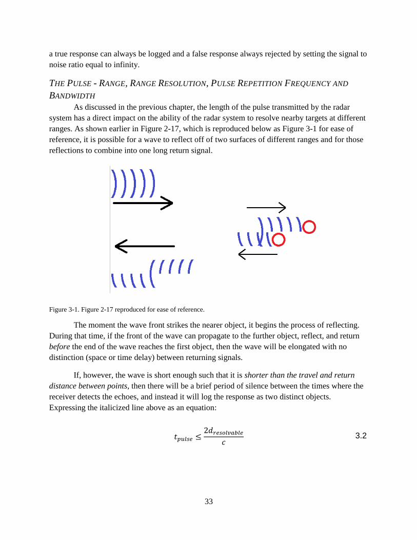
33
a true response can always be logged and a false response always rejected by setting the signal to
noise ratio equal to infinity.
THE PULSE - RANGE, RANGE RESOLUTION, PULSE REPETITION FREQUENCY AND
BANDWIDTH
As discussed in the previous chapter, the length of the pulse transmitted by the radar
system has a direct impact on the ability of the radar system to resolve nearby targets at different
ranges. As shown earlier in Figure 2-17, which is reproduced below as Figure 3-1 for ease of
reference, it is possible for a wave to reflect off of two surfaces of different ranges and for those
reflections to combine into one long return signal.
Figure 3-1. Figure 2-17 reproduced for ease of reference.
The moment the wave front strikes the nearer object, it begins the process of reflecting.
During that time, if the front of the wave can propagate to the further object, reflect, and return
before the end of the wave reaches the first object, then the wave will be elongated with no
distinction (space or time delay) between returning signals.
If, however, the wave is short enough such that it is shorter than the travel and return
distance between points, then there will be a brief period of silence between the times where the
receiver detects the echoes, and instead it will log the response as two distinct objects.
Expressing the italicized line above as an equation:
3.2
34
where tpulse is the time between the start and end of the pulse in seconds, dresolvable is the desired
resolvable distance between objects in meters, and c is the speed of wave propagation in meters
per second, e.g., the speed of light.
Another method for expressing the width of the pulse is in bandwidth, which would be
the frequency necessary for a carrier signal or window to fully envelop the pulse. Assuming the
pulse has a duration of tpulse, the period of the carrier signal that exactly covers the same length of
time must also be , and the bandwidth of the pulse is then:
3.3
Setting the resolvable distance equal to the beam width at the ideal target position gives a
reasonable approximation of a cube of space at the desired three dimensional coordinate. A
volume at a given coordinate is sometimes referred to as a voxel. A 3D image can be constructed
by logging the received signal strength for each voxel, to generate a shaded image, or can be
logged by whether or not an object exists at all in that voxel, to generate a black and white
image.
The desired maximum operating range plays a part in the radar power equation coming
up soon, as farther distances require higher signal strengths, but it also determines the minimum
time that can elapse between pulses. Ideally, signals reflecting just on the “far” side of the
desired operating range would drop immediately to the noise floor, while signals just on the
“near” side would be detectable. If this were the case, the minimum time between pulses, known
as the pulse repetition frequency (PRF), would be calculated as:
3.4
where rmax is the maximum operating range in meters and c is as defined earlier. The factor of
two comes from the fact that the signal must travel from the transmitter, to the target, then back
to the receiver.
The frequency given in Equation 3.4 is the highest frequency at which the pulses may be
sent. This ensures that enough time has elapsed since the previous transmission for the receiver
to have gathered all of the possible reflections. Lower frequencies represent longer elapsed time
between scans. NOTE: Do not confuse the pulse repetition frequency with the radar’s operating
frequency.
APERTURE SIZE CALCULATION
The physical size of the aperture is irrelevant with regards to the radar system, but may
have significant costs to implement in real life. As mentioned earlier, an eight element array
operating at 300 kHz will span almost 2.5 miles. The total aperture size can be calculated by:
35
( ) 3.5
where L is the aperture width in meters; N is the number of elements in the array; and d is the
space between elements in the array, in meters. The ( ) term comes from the fact that the
array length is determined by the spacing between radiators – an array of one has zero length!
The wavelength of a signal is related to the speed of propagation and frequency as shown earlier
in Equation 2.1:
3.6
where λ is the wavelength in meters, f is the frequency in hertz, and c is as defined earlier. Using
this equation and the definition of the array spacing
gives the aperture length as:
( )
3.7
It is usually easier and more cost effective to operate at higher frequencies than to have
physical apertures yards or miles wide, so the most effective way to start the system design is to
first pick the largest tolerable aperture width and then adjust the operating frequency until the
desired beam width is achieved.
BEAM WIDTH CALCULATION
The formula for the width of the main lobe for an array is derived in [14] and shown here
as:
( ) 3.8
where N is the number of elements in the array, d is the inter-element spacing, λ is the
wavelength, θsteer is the electronically steered beam direction, and HPBW stands for the half
power (-3dB) beam width, in radians.
Notice the ( ) term in Equation 3.8. This term means that the beam will
gradually widen as it is steered away from the broadside axis. The beam width is at a minimum
when it is not steered, then very slowly expands until it is twice as wide as the minimum width
when steered to ±60°, then three times the minimum width at ±70.5°, then rapidly increasing in
width as the cosecant function approaches a divide-by-zero at ±90°. Assuming the array is set up
on a half wavelength spacing, then
and Equation 3.8 reduces to:
( ) 3.9
36
This shows the beam width is determined solely by the number of elements in the array.
Recall, though, that the elements are still arranged on half wavelength intervals, so the operating
frequency, which is inversely proportional to wavelength, will determine the physical space the
array will occupy. It is important to note that the equations above give the beam width in radians.
For degrees, use Equation 3.10 below:
( ) 3.10
The term
in Equation 3.10 was purposefully separated from the 50 as a reminder that
the equation only applies for the half wavelength spaced array.
OPERATING FREQUENCY SELECTION
Once the largest tolerable physical dimensions have been set and the number of elements
required to achieve the desired beam width has been calculated, the lower limit on operating
frequency is fixed. Substituting Equation 3.10, which gives beamwidth in terms of the number of
elements in the array, into Equation 3.7, which gives the array width in terms of the number of
elements in the array and the operating wavelength, gives a formula relating beam width to
wavelength. Using the definition of wavelength from Equation 3.6 relates operating frequency to
desired beam width:
(
)(
)
3.11
where the half power beam width is in degrees and all other terms are as defined earlier. As with
Equation 3.10, the term
is left in that form rather than multiplying out the 2 as a reminder
that the equation only applies for half wavelength spaced arrays.
Notice that c is a constant, so the operating frequency is constrained by the physical size
and desired beamwidth. As mentioned above, the frequency given by Equation 3.11 is the lower
limit for operating frequency. Any frequencies lower than that given by Equation 3.11 will result
in a longer wavelength, which will force a larger physical aperture. Higher frequencies allow a
smaller physical size.
TRANSMITTER POWER ESTIMATION
The “radar equation” is one of the fundamental equations of radar system design, and it
uses most of the antenna and performance parameters to calculate the required broadcast
transmission power. The equation is derived in [22] and shown here in the following form:
( )
3.12

37
where Pt is the transmission power in watts, Pr is the received signal power in watts, Rt is the
distance from the transmitter to the target in meters, Rr is the distance from the target to the
receiver in meters, Gr is the gain of the receiver in decibels, Gt is the gain of the transmitter in
decibels, λ is the wavelength of the radar’s operating frequency in meters, and σ is the radar
cross-section (RCS) of the target in square meters.
This brings up an important point, which has not been addressed until now. The radar
system designed here is referred to as monostatic radar because the receiver and transmitter are,
in fact, the same physical device. That is, they are both in the same (mono) location (or station).
It is possible, but not addressed in this paper, for the transmitter and receiver to be located in two
different places. This is more common with weapon systems, where a high power transmitter is
located on the ground, and a low power (lightweight) receiver in something such as a torpedo or
missile can detect (and thus home in on) reflections from a target.
Knowing that the transmitter and receiver are the same device means that the distance
from the target to each must be the same, and, because they use the same antenna, each has the
same gain as well. This means that Equation 3.12 simplifies to:
( )
3.13
where all terms are as defined above for Equation 3.12.
The wavelength was fixed in the previous section, when the operating frequency was
determined. The operating frequency, in turn, was fixed by the section before that, when the
beam width and physical dimensions were chosen. The gain is fixed by the choice of antenna.
The operating range is also determined by the designer, so the only values left to determine are
the signal power at the receiver and the target’s radar cross-section.
The target’s RCS is determined largely by the geometry of the target and is discussed
more in the following chapter. There is no formula for the signal power of the echo directly, but
a formula that was already covered is the signal to noise ratio. A formula for the expected noise
exists, and is also given in [22]:
3.14
where Pnoise is the noise power in watts, k is the Boltzmann constant (1.38 x 10⁻²³
joule/degree), T
is the absolute temperature of the receiver in Kelvin, and Br is the receiver’s bandwidth in hertz.
The receiver’s bandwidth is assumed to be equal to the pulse bandwidth to ensure the pulse is
adequately sampled.
38
Now, with a way to calculate noise, and knowing that the signal to noise ratio is, well, the
ratio of signal to noise, Equation 3.13 can be restated as:
( )( )( )
3.15
where SNR is the signal to noise ratio and all other terms are as defined earlier.
THRESHOLD SELECTION
The sections above describe the characteristics of the pulse, transmitter, receiver, physical
array, and beam width. As discussed in the previous chapter and in [23], the matched filter is the
time-reversed and conjugated version of the transmitted waveform. Then, once the pulse has
been generated, transmitted, reflected, received, and filtered, the last step is to determine at what
value the recorded response is considered a true positive response.
[23] derives the formula for determining the signal power threshold:
[
( ( )) ] 3.16
where TdB is the threshold in decibels, Nsamples is the number of samples, β is the variance of the
white Gaussian noise at the receiver, erf -1
is the inverse of the error function, and Pfa is the
probability of false alarm.

39
Chapter 4 DESIGN CRITERIA, FULL SYSTEM SPECS, AND TARGETS
CHAPTER SUMMARY
This chapter discusses how the final values for system parameters are selected. Once the
parameters are established, the equations from the previous chapter are used to tabulate the full
system specifications. The design parameters revolve around the minimum detectable target, but
the performance is evaluated using a set of realistic targets in a “crowded scene.” Following the
disclosure of the full specifications, the method for approximating the realistic targets is
discussed.
SYSTEM DESIGN
OVERVIEW
The concept for the radar imager is a “magic window” that the user carries at waist level
that images objects in the ground as though the soil did not exist. This is depicted in Figure 4-1
below. The radar system scans and builds an image in real time, and there is no “search head” as
with conventional metal detectors. The radar unit can be located on the obverse of a screen that
can display the processed images.
Figure 4-1. Conceptual operation.
The minimum detector distance is that from the array to the top of the soil, or about one
meter. The maximum detector distance is an additional 18 inches, or approximately 0.5 meters

40
past the minimum distance. [24] states that anti-personnel mines, which are of primary concern
in most third world countries, “are typically buried extremely shallow,” while anti-tank mines
can be buried, “up to 16 in (40 cm) deep.”
The optimum scan range would be such that the imaged patch on the ground
corresponded exactly to the screen. Objects on the top of the soil would be rendered in 1:1 scale
in the position on the screen that they lay on the ground. The user can then look at the screen,
without having to crouch, to evaluate objects discovered, and can quickly and intuitively
determine where on the ground objects on the screen are located.
An intuitive, easy to understand interface is crucial for a device that could be shipped to
nearly every country in the world. Additionally, an easily understandable interface reduces
mistakes, which could be lethal. It is important to consider people may lose their life or limbs if
they do not understand the information presented.
The last aspect of an intuitive interface is a restatement of the thesis problem – the radar
system must be capable of producing images that are identifiable. There must not be a “look up
table” or set of representative symbols for the user to interpret. The user should be able to
determine what the object is based solely on its appearance on the screen. The resolution
requirements are explained next.
THE MINIMUM TARGET
The ideal minimum target for the imaging system was selected by evaluating expected
metal content and geometry in what is known as a minimum metal landmine. Minimum metal
mines are specifically designed to defeat demining techniques, commonly handheld pulse
induction metal detectors. Pulse induction metal detectors are the same kind used by hobby and
recreational metal detector enthusiasts.
Minimum metal mines are made almost entirely of plastic, using shear pins or Belleville
springs made of plastic to ensure a triggering threshold is met before detonation. The housing is
also made of plastic, so the only metallic component is the firing pin that stabs the explosive.
Minimum metal mines typically contain just one gram of metal, typically a steel tipped firing
pin. Other styles of landmines are manufactured entirely of plastic, using friction-sensitive
explosives or ceramics for firing pins, but even the complete lack of metal is not considered an
issue because plastics reflect well in the microwave region. [25]
The landmine can be very large relative to the size of the firing pin, but, since the point of
the imaging system is to be able to differentiate between mines and scrap, the firing pin was
selected as the “ideal” target. The system that can adequately resolve down to one gram of steel
should be able to discriminate well, and would absolutely be able to resolve the landmine in its
entirety.
41
For the purposes of establishing a beamwidth, the one gram piece of steel was assumed to
take the form of the most compact method of storing matter – a sphere. The assumption is that, if
the same mass took a different shape, the cross-sectional area would only increase, making it
more likely to detect the object. Additionally, assuming the form to be a sphere made radar
cross-section calculations possible. The formula for radar cross section is given in [26] as:
4.1
where σ is the radar cross section. The reflectivity and directivity can be determined
experimentally, but [26] goes on to assert that, “The sphere is the unique target that the RCS is
independent of the frequency.” This means that reflectivity and directivity do not need to be
determined; the cross-section of the sphere alone is sufficient.
[27] gives the density of American Iron and Steel Institute (AISI) grade 302 steel to be
8060 kg/m3. Dividing the target mass of 0.001 kg by the density of steel gives the volume of the
target as 1.24 x 10⁻⁷
m3. The formula for the volume of a sphere, solved for the sphere’s radius
below Equation 4.2 gives the radius of the 1g steel sphere as 3.09 mm.
(
)
4.2
Now, using the formula for area of a circle, below in Equation 4.3, the cross-sectional
area of the sphere is calculated to be 3.01 x 10⁻⁵
m2.
4.3 The beamwidth was calculated using the arctangent of the target radius and the expected
distance from the array. These values are shown relative to each other in Figure 4-2 below. As
shown, the arctangent will give half the required beamwidth. Equation 4.4 below gives the full
beamwidth:
(
) 4.4
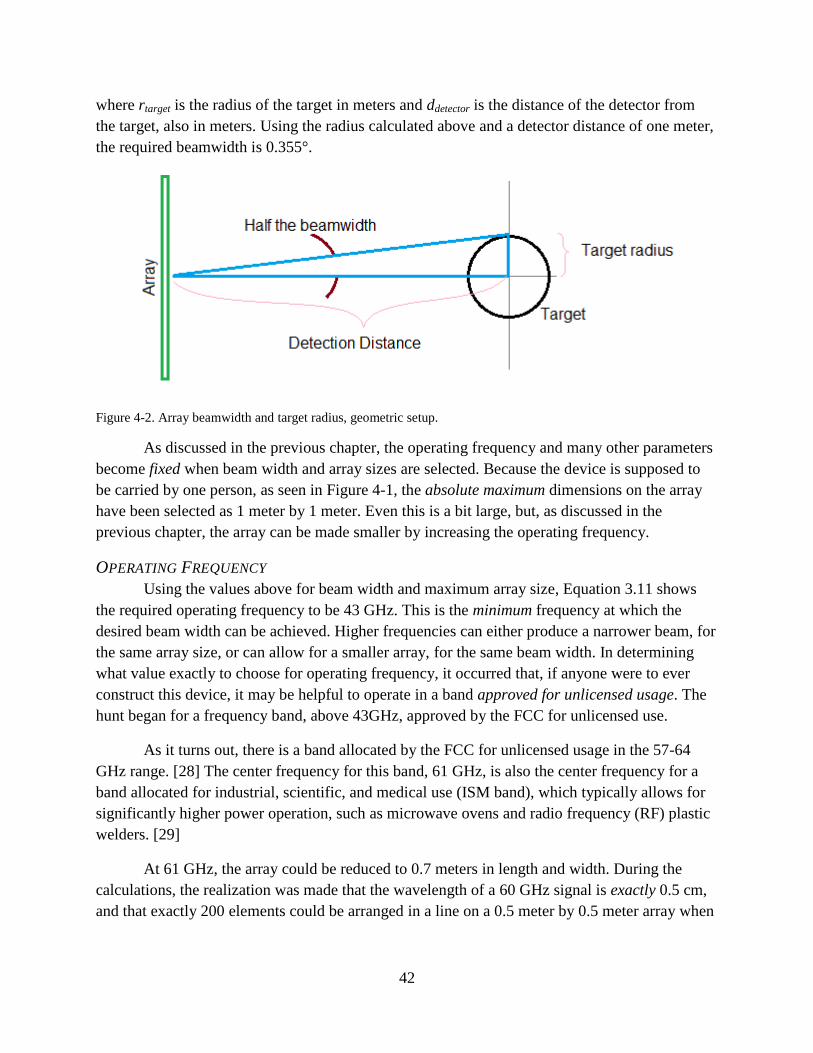
42
where rtarget is the radius of the target in meters and ddetector is the distance of the detector from
the target, also in meters. Using the radius calculated above and a detector distance of one meter,
the required beamwidth is 0.355°.
Figure 4-2. Array beamwidth and target radius, geometric setup.
As discussed in the previous chapter, the operating frequency and many other parameters
become fixed when beam width and array sizes are selected. Because the device is supposed to
be carried by one person, as seen in Figure 4-1, the absolute maximum dimensions on the array
have been selected as 1 meter by 1 meter. Even this is a bit large, but, as discussed in the
previous chapter, the array can be made smaller by increasing the operating frequency.
OPERATING FREQUENCY
Using the values above for beam width and maximum array size, Equation 3.11 shows
the required operating frequency to be 43 GHz. This is the minimum frequency at which the
desired beam width can be achieved. Higher frequencies can either produce a narrower beam, for
the same array size, or can allow for a smaller array, for the same beam width. In determining
what value exactly to choose for operating frequency, it occurred that, if anyone were to ever
construct this device, it may be helpful to operate in a band approved for unlicensed usage. The
hunt began for a frequency band, above 43GHz, approved by the FCC for unlicensed use.
As it turns out, there is a band allocated by the FCC for unlicensed usage in the 57-64
GHz range. [28] The center frequency for this band, 61 GHz, is also the center frequency for a
band allocated for industrial, scientific, and medical use (ISM band), which typically allows for
significantly higher power operation, such as microwave ovens and radio frequency (RF) plastic
welders. [29]
At 61 GHz, the array could be reduced to 0.7 meters in length and width. During the
calculations, the realization was made that the wavelength of a 60 GHz signal is exactly 0.5 cm,
and that exactly 200 elements could be arranged in a line on a 0.5 meter by 0.5 meter array when
43
spaced at half a wavelength. Once the array has been shrunk to 0.5 meters, or about 20 inches,
the device becomes very portable because this is also very close to shoulder width.
BEAM WIDTH
There was concerned at first that the ideal target would not be detectable with a larger
beam width, but then there was the realization that, as explained in Chapter 2, an object smaller
than the beam will be smeared to the same width as the beam. The transmitter power equation
from last chapter, Equation 3.15, shows that a target of any size can be detected, if the transmitter
power is set correctly. That is, even if it is not possible to resolve to the dimension of the
minimum target, it can still be detected.
At 60 GHz, the square, half-meter array produces a beam that is 0.51 degrees wide,
which is 40% wider than the beam for the ideal target, which was 0.35 degrees. However, as
previously discussed, the ideal target was the conservative estimate for required imaging
resolution. A plastic landmine would appear as a solid object [25], so achieving the 0.35° target
exactly is not necessary. The chief performance metric is discriminatory ability in a crowded
scene that would be expected in a war zone.
DETECTION PROBABILITIES
The probabilities of detection and false alarm were selected based on their physical
meaning and on common values found in radar literature. As stated in the previous chapter, the
best value for probability of detection is 1, meaning a valid target is always detected, and the best
for the probability of false alarm is 0, meaning a false target is always rejected. Without any
experience, 1 x 10⁻⁶
was selected for the probability of false alarm, as this value was given
frequently in radar literature as a commonly accepted value.
For the probability of detection, 0.99 or 0.999 were commonly chosen values, but
because of the life and death nature of minefield clearance, a value of 0.9999 was selected. This
means that, statistically speaking, one in ten thousand valid targets will be rejected. This number
seems trivial until you consider the fact that the radar is operating at the speed of light, and there
are tens of millions of pulses every second.
There is no easy way to explain why this is okay without giving away values for sections
discussed later in the paper. So, having said this, it is possible to cheat and give away some of the
information now, and you can know that the explanations for the values are “coming soon.”
There are also 9,025 pulses required to make one “scan” of the scene (akin to one “frame” of a
video). So, statistically speaking, roughly one “pixel” or “voxel” should be wrongly rejected
every scan.
If one pixel is incorrectly rejected every frame, then the odds of two pixels being wrongly
rejected on the same frame are now one in ten thousand ([ ] ). Take into account that these
pixels could be anywhere on the frame, and to have two side by side pixels would be another 1 in
9,025. Now take into account that each pixel is still only 0.2° on an edge, or about 3 mm by 3
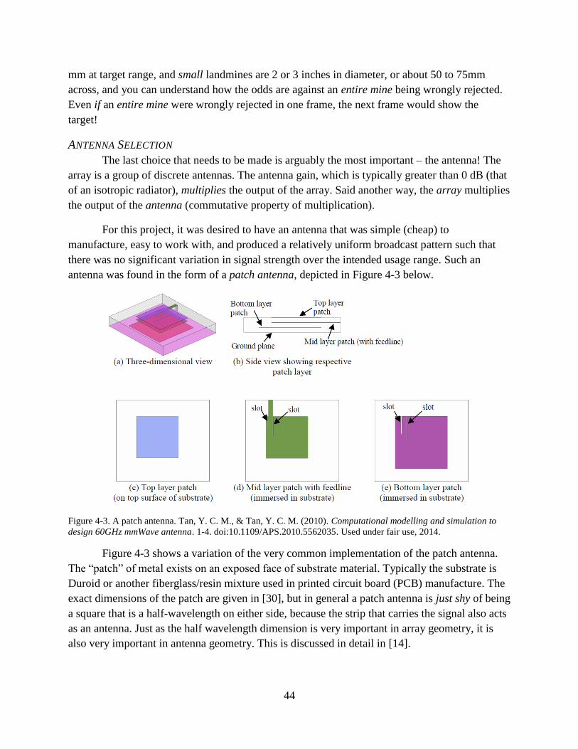
44
mm at target range, and small landmines are 2 or 3 inches in diameter, or about 50 to 75mm
across, and you can understand how the odds are against an entire mine being wrongly rejected.
Even if an entire mine were wrongly rejected in one frame, the next frame would show the
target!
ANTENNA SELECTION
The last choice that needs to be made is arguably the most important – the antenna! The
array is a group of discrete antennas. The antenna gain, which is typically greater than 0 dB (that
of an isotropic radiator), multiplies the output of the array. Said another way, the array multiplies
the output of the antenna (commutative property of multiplication).
For this project, it was desired to have an antenna that was simple (cheap) to
manufacture, easy to work with, and produced a relatively uniform broadcast pattern such that
there was no significant variation in signal strength over the intended usage range. Such an
antenna was found in the form of a patch antenna, depicted in Figure 4-3 below.
Figure 4-3. A patch antenna. Tan, Y. C. M., & Tan, Y. C. M. (2010). Computational modelling and simulation to
design 60GHz mmWave antenna. 1-4. doi:10.1109/APS.2010.5562035. Used under fair use, 2014.
Figure 4-3 shows a variation of the very common implementation of the patch antenna.
The “patch” of metal exists on an exposed face of substrate material. Typically the substrate is
Duroid or another fiberglass/resin mixture used in printed circuit board (PCB) manufacture. The
exact dimensions of the patch are given in [30], but in general a patch antenna is just shy of being
a square that is a half-wavelength on either side, because the strip that carries the signal also acts
as an antenna. Just as the half wavelength dimension is very important in array geometry, it is
also very important in antenna geometry. This is discussed in detail in [14].
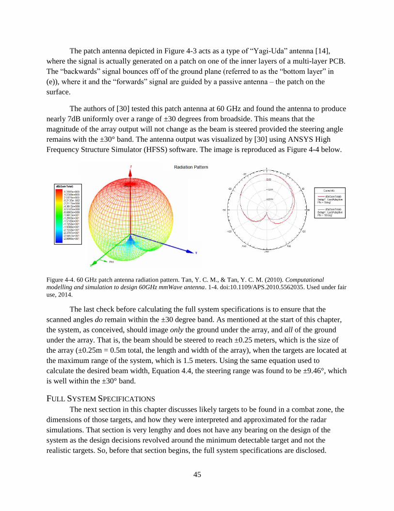
45
The patch antenna depicted in Figure 4-3 acts as a type of “Yagi-Uda” antenna [14],
where the signal is actually generated on a patch on one of the inner layers of a multi-layer PCB.
The “backwards” signal bounces off of the ground plane (referred to as the “bottom layer” in
(e)), where it and the “forwards” signal are guided by a passive antenna – the patch on the
surface.
The authors of [30] tested this patch antenna at 60 GHz and found the antenna to produce
nearly 7dB uniformly over a range of ±30 degrees from broadside. This means that the
magnitude of the array output will not change as the beam is steered provided the steering angle
remains with the ±30° band. The antenna output was visualized by [30] using ANSYS High
Frequency Structure Simulator (HFSS) software. The image is reproduced as Figure 4-4 below.
Figure 4-4. 60 GHz patch antenna radiation pattern. Tan, Y. C. M., & Tan, Y. C. M. (2010). Computational
modelling and simulation to design 60GHz mmWave antenna. 1-4. doi:10.1109/APS.2010.5562035. Used under fair
use, 2014.
The last check before calculating the full system specifications is to ensure that the
scanned angles do remain within the ±30 degree band. As mentioned at the start of this chapter,
the system, as conceived, should image only the ground under the array, and all of the ground
under the array. That is, the beam should be steered to reach ±0.25 meters, which is the size of
the array (±0.25m = 0.5m total, the length and width of the array), when the targets are located at
the maximum range of the system, which is 1.5 meters. Using the same equation used to
calculate the desired beam width, Equation 4.4, the steering range was found to be ±9.46°, which
is well within the ±30° band.
FULL SYSTEM SPECIFICATIONS
The next section in this chapter discusses likely targets to be found in a combat zone, the
dimensions of those targets, and how they were interpreted and approximated for the radar
simulations. That section is very lengthy and does not have any bearing on the design of the
system as the design decisions revolved around the minimum detectable target and not the
realistic targets. So, before that section begins, the full system specifications are disclosed.
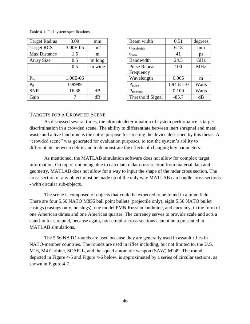
46
Table 4-1. Full system specifications.
Target Radius 3.09 mm Beam width 0.51 degrees
Target RCS 3.00E-05 m2 dresolvable 6.18 mm
Max Distance 1.5 m tpulse 41 ps
Array Size 0.5 m long Bandwidth 24.3 GHz
0.5 m wide Pulse Repeat
Frequency
100 MHz
Pfa 1.00E-06 Wavelength 0.005 m
Pd 0.9999 Pnoise 1.94 E -10 Watts
SNR 16.38 dB Ptransmit 0.109 Watts
Gain 7 dB Threshold Signal -85.7 dB
TARGETS FOR A CROWDED SCENE
As discussed several times, the ultimate determination of system performance is target
discrimination in a crowded scene. The ability to differentiate between inert shrapnel and metal
waste and a live landmine is the entire purpose for creating the device described by this thesis. A
“crowded scene” was generated for evaluation purposes, to test the system’s ability to
differentiate between debris and to demonstrate the effects of changing key parameters.
As mentioned, the MATLAB simulation software does not allow for complex target
information. On top of not being able to calculate radar cross section from material data and
geometry, MATLAB does not allow for a way to input the shape of the radar cross section. The
cross section of any object must be made up of the only way MATLAB can handle cross sections
- with circular sub-objects.
The scene is composed of objects that could be expected to be found in a mine field.
There are four 5.56 NATO M855 ball point bullets (projectile only), eight 5.56 NATO bullet
casings (casings only, no slugs), one model PMN Russian landmine, and currency, in the form of
one American dimes and one American quarter. The currency serves to provide scale and acts a
stand-in for shrapnel, because again, non-circular cross-sections cannot be represented in
MATLAB simulations.
The 5.56 NATO rounds are used because they are generally used in assault rifles in
NATO-member countries. The rounds are used in rifles including, but not limited to, the U.S.
M16, M4 Carbine, SCAR-L, and the squad automatic weapon (SAW) M249. The round,
depicted in Figure 4-5 and Figure 4-6 below, is approximated by a series of circular sections, as
shown in Figure 4-7.
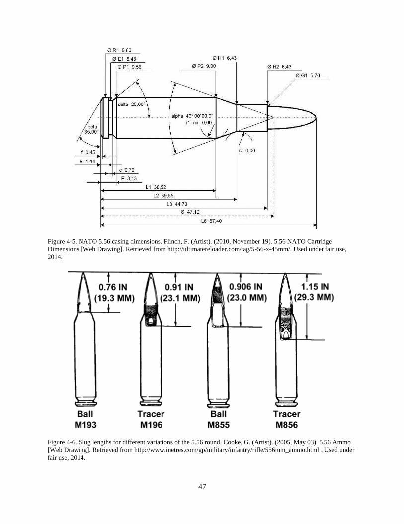
47
Figure 4-5. NATO 5.56 casing dimensions. Flinch, F. (Artist). (2010, November 19). 5.56 NATO Cartridge
Dimensions [Web Drawing]. Retrieved from http://ultimatereloader.com/tag/5-56-x-45mm/. Used under fair use,
2014.
Figure 4-6. Slug lengths for different variations of the 5.56 round. Cooke, G. (Artist). (2005, May 03). 5.56 Ammo
[Web Drawing]. Retrieved from http://www.inetres.com/gp/military/infantry/rifle/556mm_ammo.html . Used under
fair use, 2014.
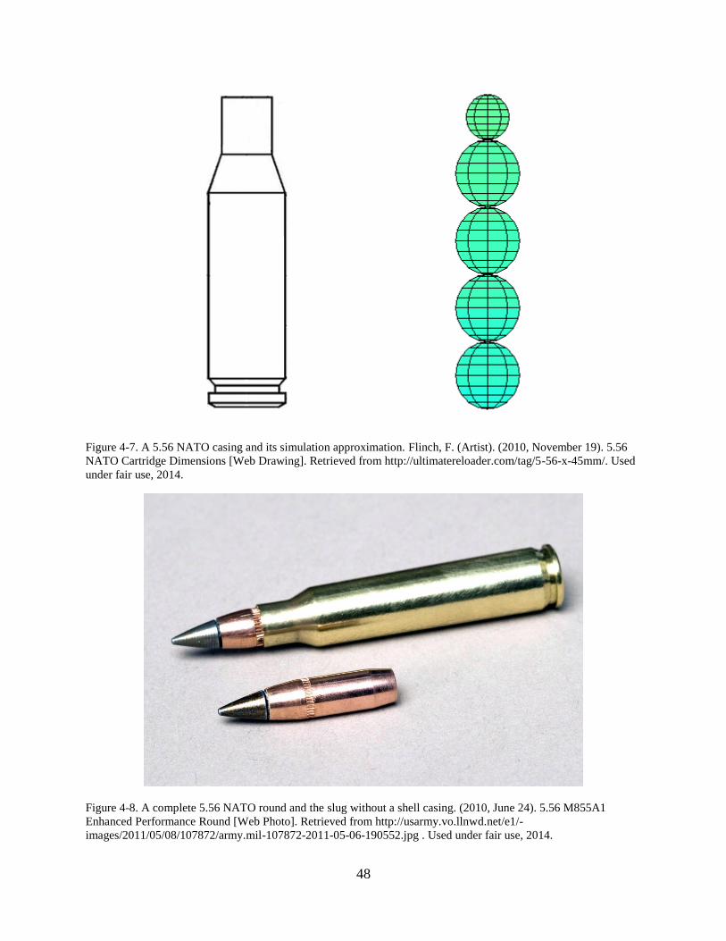
48
Figure 4-7. A 5.56 NATO casing and its simulation approximation. Flinch, F. (Artist). (2010, November 19). 5.56
NATO Cartridge Dimensions [Web Drawing]. Retrieved from http://ultimatereloader.com/tag/5-56-x-45mm/. Used
under fair use, 2014.
Figure 4-8. A complete 5.56 NATO round and the slug without a shell casing. (2010, June 24). 5.56 M855A1
Enhanced Performance Round [Web Photo]. Retrieved from http://usarmy.vo.llnwd.net/e1/-
images/2011/05/08/107872/army.mil-107872-2011-05-06-190552.jpg . Used under fair use, 2014.
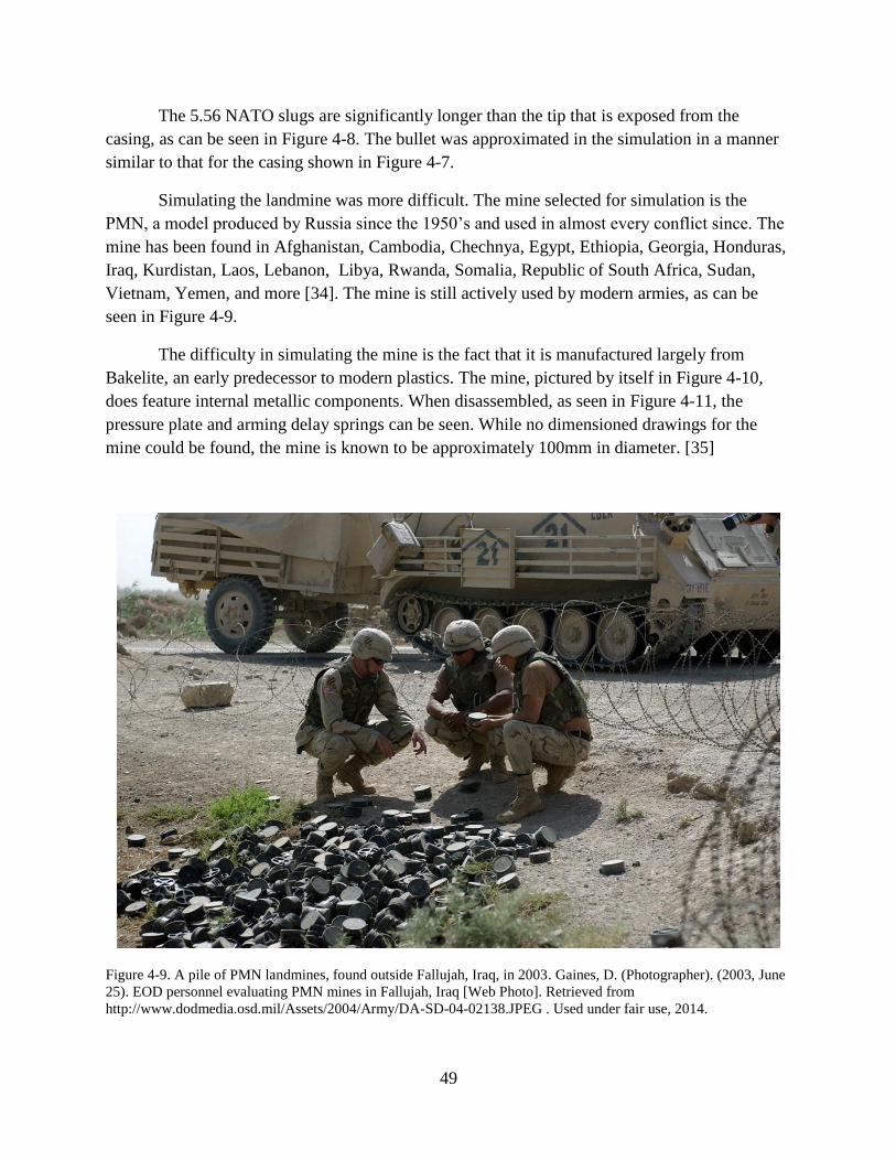
49
The 5.56 NATO slugs are significantly longer than the tip that is exposed from the
casing, as can be seen in Figure 4-8. The bullet was approximated in the simulation in a manner
similar to that for the casing shown in Figure 4-7.
Simulating the landmine was more difficult. The mine selected for simulation is the
PMN, a model produced by Russia since the 1950’s and used in almost every conflict since. The
mine has been found in Afghanistan, Cambodia, Chechnya, Egypt, Ethiopia, Georgia, Honduras,
Iraq, Kurdistan, Laos, Lebanon, Libya, Rwanda, Somalia, Republic of South Africa, Sudan,
Vietnam, Yemen, and more [34]. The mine is still actively used by modern armies, as can be
seen in Figure 4-9.
The difficulty in simulating the mine is the fact that it is manufactured largely from
Bakelite, an early predecessor to modern plastics. The mine, pictured by itself in Figure 4-10,
does feature internal metallic components. When disassembled, as seen in Figure 4-11, the
pressure plate and arming delay springs can be seen. While no dimensioned drawings for the
mine could be found, the mine is known to be approximately 100mm in diameter. [35]
Figure 4-9. A pile of PMN landmines, found outside Fallujah, Iraq, in 2003. Gaines, D. (Photographer). (2003, June
25). EOD personnel evaluating PMN mines in Fallujah, Iraq [Web Photo]. Retrieved from
http://www.dodmedia.osd.mil/Assets/2004/Army/DA-SD-04-02138.JPEG . Used under fair use, 2014.
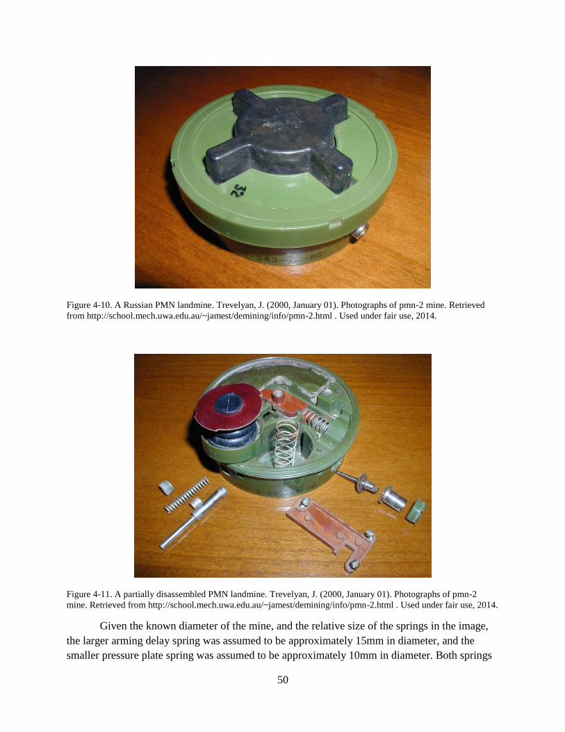
50
Figure 4-10. A Russian PMN landmine. Trevelyan, J. (2000, January 01). Photographs of pmn-2 mine. Retrieved
from http://school.mech.uwa.edu.au/~jamest/demining/info/pmn-2.html . Used under fair use, 2014.
Figure 4-11. A partially disassembled PMN landmine. Trevelyan, J. (2000, January 01). Photographs of pmn-2
mine. Retrieved from http://school.mech.uwa.edu.au/~jamest/demining/info/pmn-2.html . Used under fair use, 2014.
Given the known diameter of the mine, and the relative size of the springs in the image,
the larger arming delay spring was assumed to be approximately 15mm in diameter, and the
smaller pressure plate spring was assumed to be approximately 10mm in diameter. Both springs
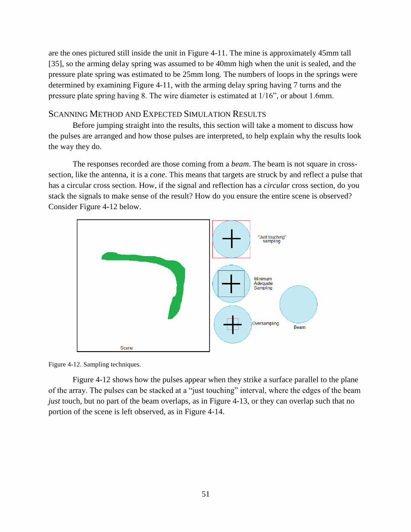
51
are the ones pictured still inside the unit in Figure 4-11. The mine is approximately 45mm tall
[35], so the arming delay spring was assumed to be 40mm high when the unit is sealed, and the
pressure plate spring was estimated to be 25mm long. The numbers of loops in the springs were
determined by examining Figure 4-11, with the arming delay spring having 7 turns and the
pressure plate spring having 8. The wire diameter is estimated at 1/16”, or about 1.6mm.
SCANNING METHOD AND EXPECTED SIMULATION RESULTS
Before jumping straight into the results, this section will take a moment to discuss how
the pulses are arranged and how those pulses are interpreted, to help explain why the results look
the way they do.
The responses recorded are those coming from a beam. The beam is not square in cross-
section, like the antenna, it is a cone. This means that targets are struck by and reflect a pulse that
has a circular cross section. How, if the signal and reflection has a circular cross section, do you
stack the signals to make sense of the result? How do you ensure the entire scene is observed?
Consider Figure 4-12 below.
Figure 4-12. Sampling techniques.
Figure 4-12 shows how the pulses appear when they strike a surface parallel to the plane
of the array. The pulses can be stacked at a “just touching” interval, where the edges of the beam
just touch, but no part of the beam overlaps, as in Figure 4-13, or they can overlap such that no
portion of the scene is left observed, as in Figure 4-14.
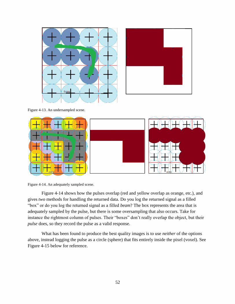
52
Figure 4-13. An undersampled scene.
Figure 4-14. An adequately sampled scene.
Figure 4-14 shows how the pulses overlap (red and yellow overlap as orange, etc.), and
gives two methods for handling the returned data. Do you log the returned signal as a filled
“box” or do you log the returned signal as a filled beam? The box represents the area that is
adequately sampled by the pulse, but there is some oversampling that also occurs. Take for
instance the rightmost column of pulses. Their “boxes” don’t really overlap the object, but their
pulse does, so they record the pulse as a valid response.
What has been found to produce the best quality images is to use neither of the options
above, instead logging the pulse as a circle (sphere) that fits entirely inside the pixel (voxel). See
Figure 4-15 below for reference.
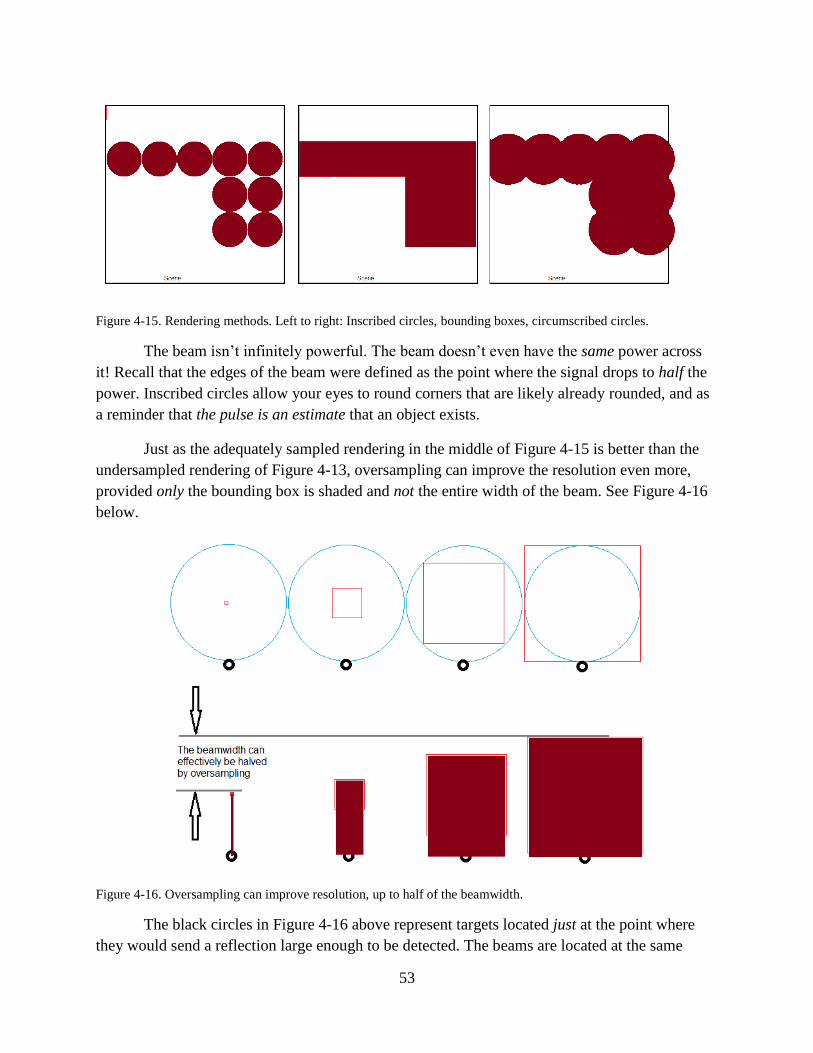
53
Figure 4-15. Rendering methods. Left to right: Inscribed circles, bounding boxes, circumscribed circles.
The beam isn’t infinitely powerful. The beam doesn’t even have the same power across
it! Recall that the edges of the beam were defined as the point where the signal drops to half the
power. Inscribed circles allow your eyes to round corners that are likely already rounded, and as
a reminder that the pulse is an estimate that an object exists.
Just as the adequately sampled rendering in the middle of Figure 4-15 is better than the
undersampled rendering of Figure 4-13, oversampling can improve the resolution even more,
provided only the bounding box is shaded and not the entire width of the beam. See Figure 4-16
below.
Figure 4-16. Oversampling can improve resolution, up to half of the beamwidth.
The black circles in Figure 4-16 above represent targets located just at the point where
they would send a reflection large enough to be detected. The beams are located at the same
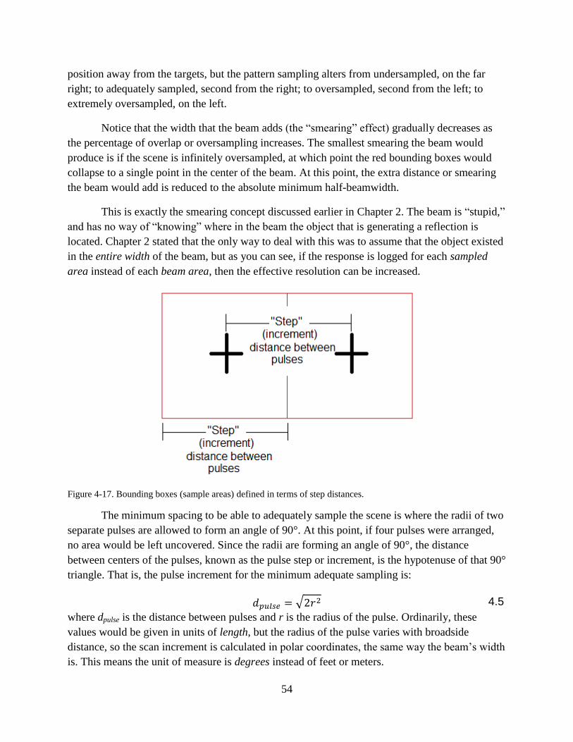
54
position away from the targets, but the pattern sampling alters from undersampled, on the far
right; to adequately sampled, second from the right; to oversampled, second from the left; to
extremely oversampled, on the left.
Notice that the width that the beam adds (the “smearing” effect) gradually decreases as
the percentage of overlap or oversampling increases. The smallest smearing the beam would
produce is if the scene is infinitely oversampled, at which point the red bounding boxes would
collapse to a single point in the center of the beam. At this point, the extra distance or smearing
the beam would add is reduced to the absolute minimum half-beamwidth.
This is exactly the smearing concept discussed earlier in Chapter 2. The beam is “stupid,”
and has no way of “knowing” where in the beam the object that is generating a reflection is
located. Chapter 2 stated that the only way to deal with this was to assume that the object existed
in the entire width of the beam, but as you can see, if the response is logged for each sampled
area instead of each beam area, then the effective resolution can be increased.
Figure 4-17. Bounding boxes (sample areas) defined in terms of step distances.
The minimum spacing to be able to adequately sample the scene is where the radii of two
separate pulses are allowed to form an angle of 90°. At this point, if four pulses were arranged,
no area would be left uncovered. Since the radii are forming an angle of 90°, the distance
between centers of the pulses, known as the pulse step or increment, is the hypotenuse of that 90°
triangle. That is, the pulse increment for the minimum adequate sampling is:
√ 4.5
where dpulse is the distance between pulses and r is the radius of the pulse. Ordinarily, these
values would be given in units of length, but the radius of the pulse varies with broadside
distance, so the scan increment is calculated in polar coordinates, the same way the beam’s width
is. This means the unit of measure is degrees instead of feet or meters.

55
Using this formula, which is really just a restatement of the Pythagorean Theorem, and
the radar system’s actual beam width of 0.51°, the minimum adequate pulse spacing is 0.36°. In
the simulations, oversampling has been performed by reducing the spacing to 0.2°.
The tradeoff between physical size and a frequency open to unlicensed use put the
beamwidth wider than desired, but, as demonstrated above, the effective beam width can be
reduced by up to half by increasing the number of samples taken. The design decisions produced
a beam that is 40% larger than desired, but the use of oversampling will compensate for the
increase in width, as will be seen during the discussion of the simulation results in the next
chapter.
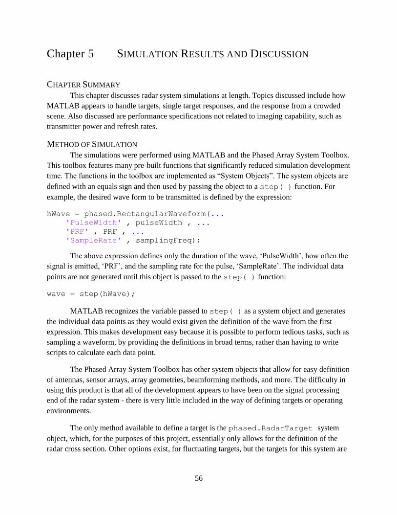
56
Chapter 5 SIMULATION RESULTS AND DISCUSSION
CHAPTER SUMMARY
This chapter discusses radar system simulations at length. Topics discussed include how
MATLAB appears to handle targets, single target responses, and the response from a crowded
scene. Also discussed are performance specifications not related to imaging capability, such as
transmitter power and refresh rates.
METHOD OF SIMULATION
The simulations were performed using MATLAB and the Phased Array System Toolbox.
This toolbox features many pre-built functions that significantly reduced simulation development
time. The functions in the toolbox are implemented as “System Objects”. The system objects are
defined with an equals sign and then used by passing the object to a step( ) function. For
example, the desired wave form to be transmitted is defined by the expression:
hWave = phased.RectangularWaveform(... 'PulseWidth' , pulseWidth , ... 'PRF' , PRF , ... 'SampleRate' , samplingFreq);
The above expression defines only the duration of the wave, ‘PulseWidth’, how often the
signal is emitted, ‘PRF’, and the sampling rate for the pulse, ‘SampleRate’. The individual data
points are not generated until this object is passed to the step( ) function:
wave = step(hWave);
MATLAB recognizes the variable passed to step( ) as a system object and generates
the individual data points as they would exist given the definition of the wave from the first
expression. This makes development easy because it is possible to perform tedious tasks, such as
sampling a waveform, by providing the definitions in broad terms, rather than having to write
scripts to calculate each data point.
The Phased Array System Toolbox has other system objects that allow for easy definition
of antennas, sensor arrays, array geometries, beamforming methods, and more. The difficulty in
using this product is that all of the development appears to have been on the signal processing
end of the radar system - there is very little included in the way of defining targets or operating
environments.
The only method available to define a target is the phased.RadarTarget system
object, which, for the purposes of this project, essentially only allows for the definition of the
radar cross section. Other options exist, for fluctuating targets, but the targets for this system are
57
non-fluctuating, so they do not apply. While it is possible to define a radar cross section, it is not
possible to input specific geometry. The impact of this will be discussed later in this chapter.
The only option for propagation is the phased.FreeSpace system object. This means
that it is not possible to immediately simulate any environment other than a vacuum. It is not
possible to simulate the effects of environmental attenuation without either writing a system
object from scratch, finding a way to correctly manipulate the output of the array to simulate the
effects, or finding a different way to simulate the system altogether. As will be discussed later, in
Chapter 6, this issue was side-stepped entirely by ignoring the effects of environmental
attenuation.
NON-IMAGING SPECIFICATIONS
TRANSMISSION POWER
The array was first simulated using pulse integration to determine the effects of multiple
pulses on system performance. Using 16 pulses for the pulse integration, the peak power for each
element was 0.2495μW. With the array being a 200x200 grid of patch antennas, this means that
the total array’s transmit power is 9.98mW. The FCC transmitter power limit, fed into the
antenna, is 500mW [28], meaning that there is plenty of headroom to increase the transmission
power. This reduces the revisit time for each location, which in turn can increase the “refresh
rate” of the imaging system.
Reducing the number of integrating pulses from 16 to 4 increased the peak power
required to achieve an adequate SNR from a total 2.495mW to 29.5mW. Reducing it again from
4 to 1 increased the peak power to a total of 109mW, which is still well within the FCC
transmission limits. Performing pulse integration may be necessary for radar units with a much
larger operating range, but the limited range of this application significantly reduces the amount
of atmospheric attenuation, which in turn limits the SNR required to ensure proper received
signal processing.
There was no difference in imaging capability when the number of pulses to integrate
was varied. This was surprising at the time, but then it quickly dawned that the entire point of
pulse integration was to achieve the desired signal to noise ratio! MATLAB was adjusting the
transmitter power automatically as the number of pulse samples was changed.
REVISIT TIME
As discussed last chapter, imaging the entire scene involves scanning ±9.46° across the
width (azimuth scan), and ±9.46° across the height (elevation scan), and the scan pattern is
utilizing moderate oversampling, scanning on a 0.2° increment. To scan the entire width means
scanning (9.46 x 2) = 18.92°. With the given increment between scans, there are 94.6 pulses to
scan one line. As there cannot be a fractional pulse, 95 pulses are required in each direction,
giving the total number of pulses to scan the scene one time to be 9,025.
58
The pulse repetition frequency is 100MHz, meaning that 100 million pulses can be
generated every second while maintaining the desired operating specifications. At that rate, given
the number of pulses to scan the scene one time, the array can scan the entire scene and then
return the beam back to the starting position to begin another scan in 6.76μs.
At this rate, the scene could be updated at a rate of 147.8 kHz. This is far above the
traditional 30 frames per second (FPS), but does not take into account the processing time
involved in calculating the next scan angle, adjusting the phase shifters, or processing the
recorded data from the receivers. The low revisit time (high revisit frequency) does suggest that
there is ample time to perform the actions described and still maintain a “real time” 30 fps
refresh rate.
SMALL SCENE RESPONSE
Before heading straight to the crowded scene response, this section will take a moment to
review the small scene responses under varying conditions to discuss and reinforce the radar
principles that have been covered throughout this paper.
VARYING SCAN STEP SIZE
The first single target response goes a long ways towards reinforcing the discussion at the
end of the previous chapter, regarding methods of interpreting pulse response data. The images
below all represent the same set of targets, three targets in a row, but the difference is the scan
spacing.
As can be seen in Figure 5-1 through Figure 5-4, oversampling can contribute a lot
towards resolution. The impact of oversampling the scan was actually far more significant than
expected before running these simulations. Oversampling generates images of far higher quality
than initially estimated. Figure 5-1 is undersampled, and the targets are so poorly represented
that they actually appear as four objects instead of one. Or, if the bounding box method is used
instead of inscribed circles, the three objects would be represented as one wide rectangle.
Oversampling improves image fidelity by increasing the number of sample points. This
improves the odds of finding a location where no object can be detected. Refer to Figure 5-4
below and notice that the objects on the left and right are separated from the one in the middle by
a width of one pixel. Oversampling also improves the appearance of the contours of the objects
because again, there are more chances to find the exact spot where the object is no longer
detectable.
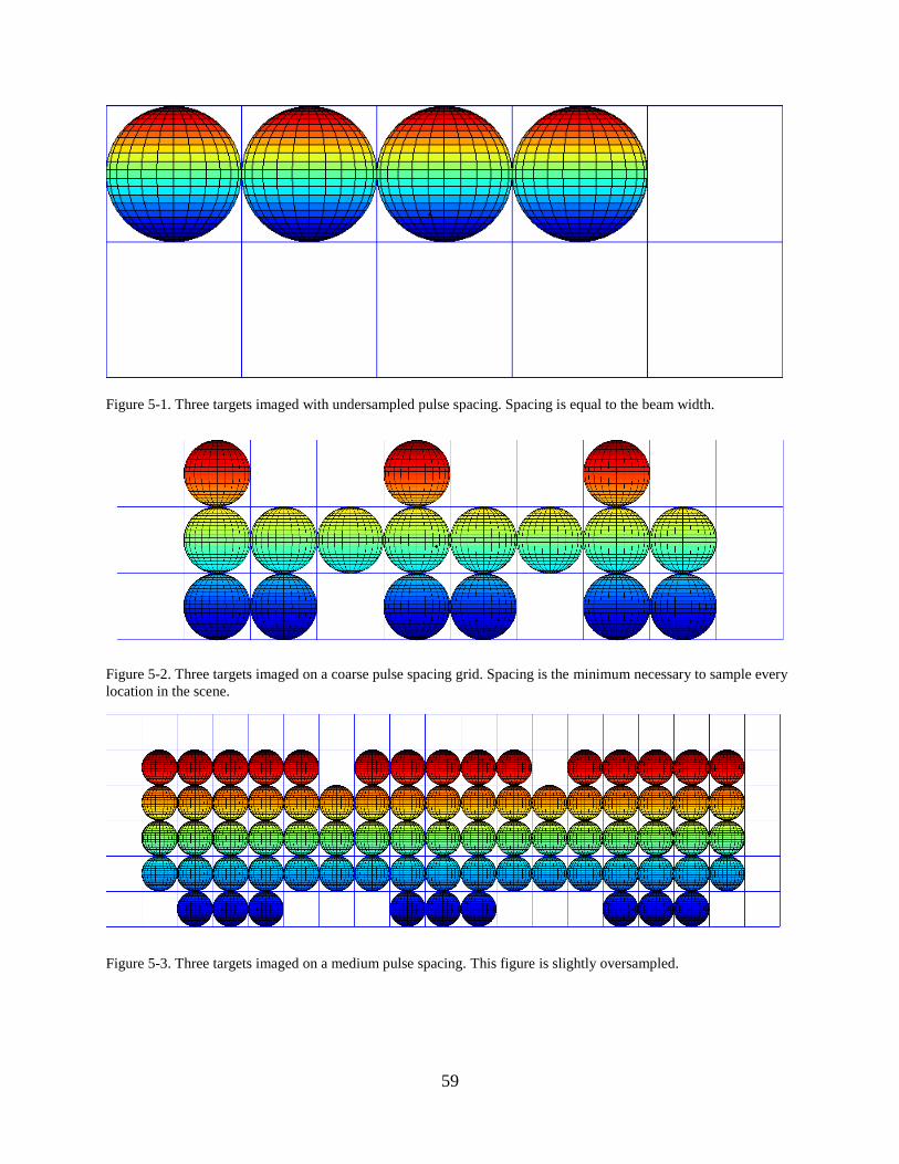
59
Figure 5-1. Three targets imaged with undersampled pulse spacing. Spacing is equal to the beam width.
Figure 5-2. Three targets imaged on a coarse pulse spacing grid. Spacing is the minimum necessary to sample every
location in the scene.
Figure 5-3. Three targets imaged on a medium pulse spacing. This figure is slightly oversampled.
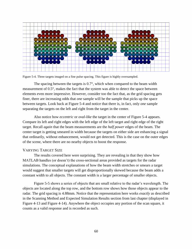
60
Figure 5-4. Three targets imaged on a fine pulse spacing. This figure is highly oversampled.
The spacing between the targets is 0.7°, which when compared to the beam width
measurement of 0.5°, makes the fact that the system was able to detect the space between
elements even more impressive. However, consider too the fact that, as the grid spacing gets
finer, there are increasing odds that one sample will be the sample that picks up the space
between targets. Look back at Figure 5-4 and notice that there is, in fact, only one sample
separating the targets on the left and right from the target in the center.
Also notice how eccentric or oval-like the target in the center of Figure 5-4 appears.
Compare its left and right edges with the left edge of the left target and right edge of the right
target. Recall again that the beam measurements are the half power edges of the beam. The
center target is getting smeared in width because the targets on either side are enhancing a signal
that ordinarily, without enhancement, would not get detected. This is the case on the outer edges
of the scene, where there are no nearby objects to boost the response.
VARYING TARGET SIZE
The results covered here were surprising. They are revealing in that they show how
MATLAB handles (or doesn’t) the cross-sectional areas provided as targets for the radar
simulations. The conceptual explanations of how the beam width stretches or smears a target
would suggest that smaller targets will get disproportionally skewed because the beam adds a
constant width to all objects. The constant width is a larger percentage of smaller objects.
Figure 5-5 shows a series of objects that are small relative to the radar’s wavelength. The
objects are located along the top row, and the bottom row shows how those objects appear to the
radar. The grid spacing is 4.88mm. Notice that the representation here works exactly as described
in the Scanning Method and Expected Simulation Results section from last chapter (displayed in
Figure 4-13 and Figure 4-14). Anywhere the object occupies any portion of the scan square, it
counts as a valid response and is recorded as such.

61
Figure 5-5. Small objects, above, and their representations, below, on a 4.88mm grid
This was the expected behavior. The hope was to be able to generate a plot that showed
the percent enlargement of objects, in terms of their width in wavelengths. As larger objects were
imaged, as seen in Figure 5-6, the pattern seemed to stop. The object 5 wavelengths (λ) across
seemed to be represented okay, but the 6λ and 8λ objects appeared to be the same sizes! More
than appearing the same size, the representations were smaller than the actual objects.
Figure 5-6. Large objects, above, and their representations, below, on a 4.88mm grid.
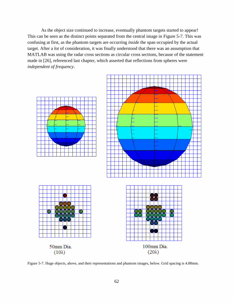
62
As the object size continued to increase, eventually phantom targets started to appear!
This can be seen as the distinct points separated from the central image in Figure 5-7. This was
confusing at first, as the phantom targets are occurring inside the span occupied by the actual
target. After a lot of consideration, it was finally understood that there was an assumption that
MATLAB was using the radar cross sections as circular cross sections, because of the statement
made in [26], referenced last chapter, which asserted that reflections from spheres were
independent of frequency.
Figure 5-7. Huge objects, above, and their representations and phantom images, below. Grid spacing is 4.88mm.

63
Instead of assuming any physical shape, MATLAB is instead using the cross section as a
value, and assigning that value to one point in space. Imagine an infinitely small reflecting lens
of varying focusing power. The radar cross section equation, Equation 4.1, gave the formula as
the physical cross section, multiplied by a reflectivity and directivity factor.
When the object is small, it approximates a point in space, and the representation is
accurate. However, as the object increases in size, MATLAB’s interpretation of the radar cross
section no longer adequately represents the true target, and the result is the distortion of the
target in the returned signal.
CROWDED SCENE RESPONSE
Having run through the simulation basics with the small scenes and individual targets,
now it’s time for the full crowded scene responses! The objects are all relatively small, so the
distortion effects discussed in the last section are not an issue here, though they would be if a
different target set were selected (like the housing of a landmine). The first figure below is the
scene itself – the objects to be imaged. This image is likely not to scale for you, so sections of the
figure will be removed from the image later so they may be displayed at a 1:1 scale, as they
would appear on the imaging system.
The targets are arranged in Figure 5-8 are as follows: NATO 5.56 shell casings are
aligned vertically, NATO 5.56 slugs are arranged horizontally, the two coins, dime and quarter,
are approximately centered horizontally, and the springs for the landmine are located in the
bottom right hand corner.
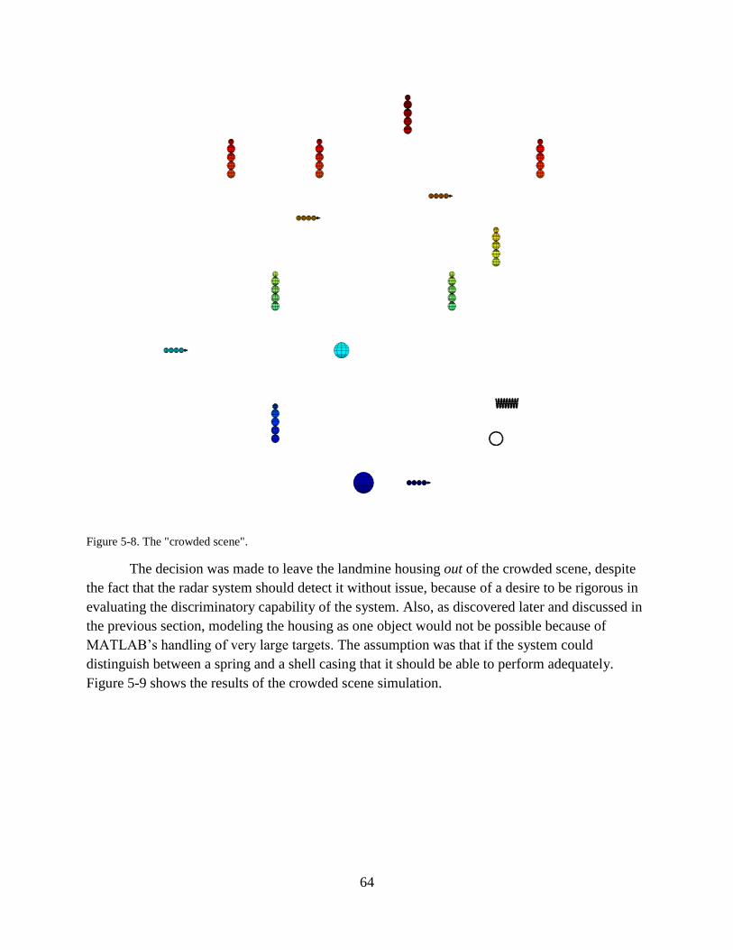
64
Figure 5-8. The "crowded scene".
The decision was made to leave the landmine housing out of the crowded scene, despite
the fact that the radar system should detect it without issue, because of a desire to be rigorous in
evaluating the discriminatory capability of the system. Also, as discovered later and discussed in
the previous section, modeling the housing as one object would not be possible because of
MATLAB’s handling of very large targets. The assumption was that if the system could
distinguish between a spring and a shell casing that it should be able to perform adequately.
Figure 5-9 shows the results of the crowded scene simulation.
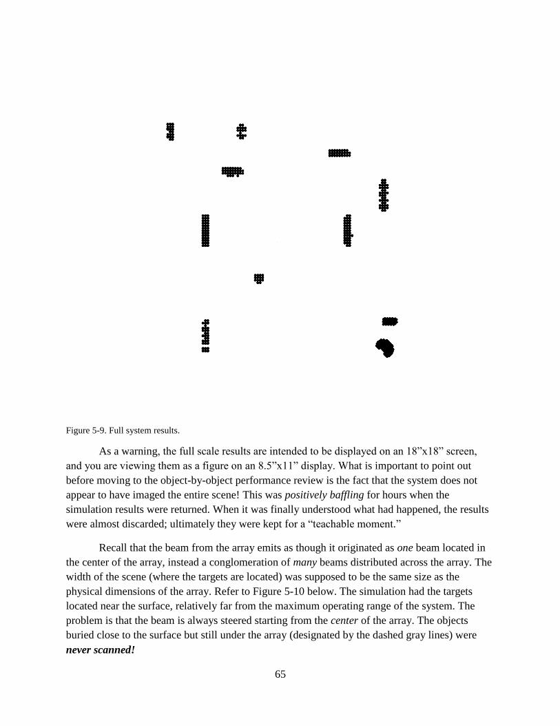
65
Figure 5-9. Full system results.
As a warning, the full scale results are intended to be displayed on an 18”x18” screen,
and you are viewing them as a figure on an 8.5”x11” display. What is important to point out
before moving to the object-by-object performance review is the fact that the system does not
appear to have imaged the entire scene! This was positively baffling for hours when the
simulation results were returned. When it was finally understood what had happened, the results
were almost discarded; ultimately they were kept for a “teachable moment.”
Recall that the beam from the array emits as though it originated as one beam located in
the center of the array, instead a conglomeration of many beams distributed across the array. The
width of the scene (where the targets are located) was supposed to be the same size as the
physical dimensions of the array. Refer to Figure 5-10 below. The simulation had the targets
located near the surface, relatively far from the maximum operating range of the system. The
problem is that the beam is always steered starting from the center of the array. The objects
buried close to the surface but still under the array (designated by the dashed gray lines) were
never scanned!
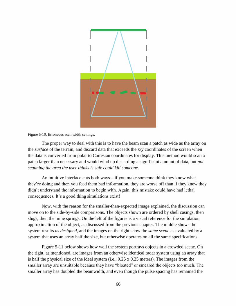
66
Figure 5-10. Erroneous scan width settings.
The proper way to deal with this is to have the beam scan a patch as wide as the array on
the surface of the terrain, and discard data that exceeds the x/y coordinates of the screen when
the data is converted from polar to Cartesian coordinates for display. This method would scan a
patch larger than necessary and would wind up discarding a significant amount of data, but not
scanning the area the user thinks is safe could kill someone.
An intuitive interface cuts both ways – if you make someone think they know what
they’re doing and then you feed them bad information, they are worse off than if they knew they
didn’t understand the information to begin with. Again, this mistake could have had lethal
consequences. It’s a good thing simulations exist!
Now, with the reason for the smaller-than-expected image explained, the discussion can
move on to the side-by-side comparisons. The objects shown are ordered by shell casings, then
slugs, then the mine springs. On the left of the figures is a visual reference for the simulation
approximation of the object, as discussed from the previous chapter. The middle shows the
system results as designed, and the images on the right show the same scene as evaluated by a
system that uses an array half the size, but otherwise operates on all the same specifications.
Figure 5-11 below shows how well the system portrays objects in a crowded scene. On
the right, as mentioned, are images from an otherwise identical radar system using an array that
is half the physical size of the ideal system (i.e., 0.25 x 0.25 meters). The images from the
smaller array are unsuitable because they have “bloated” or smeared the objects too much. The
smaller array has doubled the beamwidth, and even though the pulse spacing has remained the
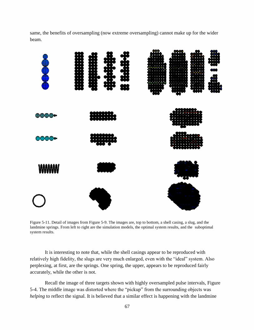
67
same, the benefits of oversampling (now extreme oversampling) cannot make up for the wider
beam.
Figure 5-11. Detail of images from Figure 5-9. The images are, top to bottom, a shell casing, a slug, and the
landmine springs. From left to right are the simulation models, the optimal system results, and the suboptimal
system results.
It is interesting to note that, while the shell casings appear to be reproduced with
relatively high fidelity, the slugs are very much enlarged, even with the “ideal” system. Also
perplexing, at first, are the springs. One spring, the upper, appears to be reproduced fairly
accurately, while the other is not.
Recall the image of three targets shown with highly oversampled pulse intervals, Figure
5-4. The middle image was distorted where the “pickup” from the surrounding objects was
helping to reflect the signal. It is believed that a similar effect is happening with the landmine

68
springs. The upper spring, from the user’s view (and the radar’s view!) appears very much like a
solid block. Indeed, to the radar, the surrounding objects will help reflect the waves and the
upper spring will return a signal exactly like a solid block.
Meanwhile, the lower spring in the bottom center of Figure 5-11 and the slugs in center
of the same figure are badly distorted. This is believed to be entirely due to the relative thinness
of the objects. Recall the discussions throughout the paper about smearing. The objects’ thin
widths cause them to appear to have a much more significant enlargement. It was not as
noticeable for the shell casings because it was a smaller percent increase in each direction, so the
aspect ratio was left largely unchanged. Notice that the slugs appear to have the correct length;
it’s just the width that appears to have changed! Similarly, because the “walls” of the lower
spring appear so thin they are significantly altered when scanned from this direction.
It is possible to increase the oversampling to correct for the extra “weight” the radar
system is putting on thin objects, but this is very likely not necessary. The goal of this system is
not to be able to identify every object in the ground! The goal is to be able to quickly and with
high certainty differentiate between landmines and scrap. The landmines were simulated as
springs to be able to evaluate discriminatory capability. It is expected that landmines would show
up in the field as large cylinders.

69
Chapter 6 LIMITATIONS AND FUTURE WORK
CHAPTER SUMMARY
This chapter points out limitations on the system design, including limitations imposed
by the simulation capabilities and limitations due to implementation aspects that were not
considered as constraints on the system design. Health and safety considerations are discussed,
and notes regarding the construction of the imaging system are addressed.
HEALTH AND SAFETY CONSIDERATIONS
The purpose of this thesis was to determine the feasibility of a high resolution, low range
ground-penetrating radar. While practicality is desirable, and all operating parameters were
guided by practical limits, the scope of this work was not to perform a complete analysis on a
finished, physical product.
Even with such a disclaimer, the author would like to go further and clearly state that this
design has not been evaluated for fitness of use. Constructing and operating the device
described in this document could lead to equipment damage, injury, and/or death.
There has not been any research into the health effects of high frequency electromagnetic
radiation, so it cannot be emphasized enough that there could be considerable risk in operating a
radar unit at waist level.
For comparison, consider a microwave oven and a wireless internet router. It would be
generally considered dangerous to operate a microwave oven without the shielded door installed
and closed, yet most internet routers are located in occupied living spaces, typically near a
computer user and/or the computer itself.
The microwave oven operates on an ISM band, at 2.45 GHz, as does the wireless router
[38][39], yet one is considered dangerous while the other is not. The microwave oven operates at
1.25 kW [38], while the wireless router has a broadcast power limit of 1W [28]. Clearly the
microwave oven has a significantly higher radiative output than the wireless router, but the
microwave oven is contained and self-shielded. The FCC has set broadcast power limits on
devices such as the wireless router so that they will not generate a signal strong enough to
endanger people or disrupt electronic devices.
At some point above 1W, a 2.45 GHz signal becomes disruptive and then destructive to
electronic and organic objects in the surrounding area. Similarly, there is a point at which any
radiated signal will become hazardous to those around it. The array power emission was
designed to stay below the FCC’s 57-64 GHz band output power limit of 500 mW [28]. There is
a lot of effort being put forth to shift wireless internet communications to 60 GHz [40] [41], and,
“60 GHz is considered the most promising technology to deliver gigabit wireless for indoor

70
communications.” [42] It is hoped that the device would be safe, but hope and expectations are
not an acceptable substitute for a safety analysis.
PROPAGATION MODELS AND NOISE
The primary purpose of performing this research was to determine if the necessary
resolution for a handheld radar system could be achieved. To that end, the simulations were
performed in an overly idealized environment - a perfect vacuum with no other objects located
nearby. Signal fade was discussed briefly in Chapter 2 as being partly due to distance from the
radiator and partly due to the attenuation of the signal by the environment.
For several reasons, the attenuation of the signal by the environment was ignored while
performing the simulations. First, MATLAB does not have a mechanism for assigning the
impedance of the environment. It is possible to simulate the effects of environmental signal
attenuation by modifying the received signal data, but doing so posed a significant development
task that did not contribute to the completion of the research project.
Secondly, the impedance of ground varies greatly. The net effect of impedance is that the
signal is essentially shorted. Given the discussion of wavelengths earlier in the paper, for any
signal, a signal with the same magnitude but opposite sign can be found half a wavelength away.
For most radar systems, which are very high frequency, this represents a very small distance. For
the designed system specifically, that distance is 2.5 mm.
The lower the impedance of the environment, the less resistance there is for those two
negating signals to short to each other and cancel. The impedance of dry air is different than that
of moist air, dry soil is different than damp soil, and impedances vary between soil types: loam,
sand, peat, clay, etc.
If the effort to develop a mechanism for including environmental impedance was
undertaken, it would only make sense to then use it to simulate the anticipated operating
environment. The radar system could be used world-wide, from the jungles of Cambodia to the
deserts of Egypt, meaning that every conceivable terrain type could be encountered. As with
implementing the mechanism to begin with, this task represented a significant development
effort with no contribution to the primary purpose of the research project: to determine if physics
even allows such a device at all.
Along the same lines, background noise was not taken into consideration. Thermal noise
was the only consideration for noise power when evaluation transmitter power and the required
signal to noise ration needed for reasonable system performance. In reality, objects located
beyond the maximum operating range will still present reflected signals to the array, even if
those signals are below the detectable threshold.
As with any noise, those faint returns can either be in-phase and constructively interfere,
creating false alarms, or can be out-of-phase and destructively interfere, causing legitimate

71
signals to be missed. The impact of this noise and noise from other emitters was neglected for the
purposes of this research project. If taken into account, this source of noise would surely require
the transmission power of the radar system to be increased. Given the current transmission power
of 0.11 W and the FCC broadcast limit of 0.5 W, there is a potential to boost the output power of
the array by approximately 6 dB while remaining under the broadcast limits.
SIMULATION LIMITATIONS
Health and safety concerns are a key issue for anyone attempting to construct and operate
the device described above, but a difficulty in evaluating the physical device would be
comparing the results of an actual imaging system to the simulation results shown in Chapter 5.
This is because MATLAB does not allow for complex target definitions, and thus all targets
were required to be approximated.
The ideal method for defining a scene would be to specify object geometry and volume,
then specify the material type or impedance, and have MATLAB simulate the wave interaction
at the interface between material types.
With such a method, it would be possible to create an environment wherein the array
operated in air, and metal targets were located in soil. This is not the case, and as such, the effect
of such air/soil and soil/metal interfaces cannot be adequately simulated. These interface
interactions would weaken, sometimes significantly, the wave as it passed the interface. This
weakening effect would occur both times the wave front passed, once on transmission and once
on reflection.
The inability of MATLAB to account for these interactions produced images that are
surely clearer than could be expected from live data. The signal could be refined with the use of
pulse integration, but the tradeoff would come at a reduced refresh rate. Given the current revisit
rate of 147 kHz, there could be dozens or hundreds of pulses used for noise reduction and still
maintain a 30Hz refresh rate. The radar is handheld, not on a jet, and the target is stationary, not
a missile, so the extreme refresh rates needed by military radars are not necessary; 30Hz should
be sufficient.
The exact gains in signal fidelity or increases in signal penetration cannot be calculated
exactly because, again, the nature of the signal interaction at the interfaces is not known. A
signal with no noise has an infinite (undefined) signal to noise ratio, and similarly, a known
signal with an unknown noise profile has an undefined signal to noise ratio. Ultimately, the
signal to noise ratio will determine effective depths, revisit (refresh) times, and overall
usefulness, but this is something that would need a constructed device and extensive field testing
to determine.
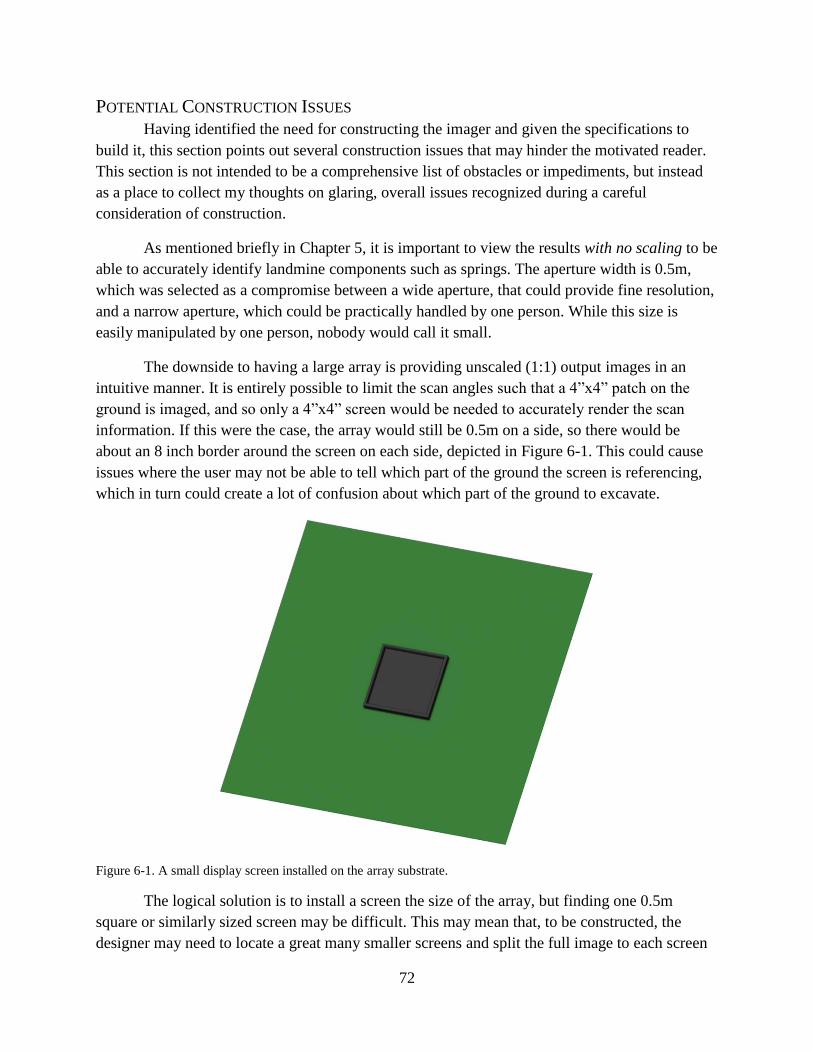
72
POTENTIAL CONSTRUCTION ISSUES
Having identified the need for constructing the imager and given the specifications to
build it, this section points out several construction issues that may hinder the motivated reader.
This section is not intended to be a comprehensive list of obstacles or impediments, but instead
as a place to collect my thoughts on glaring, overall issues recognized during a careful
consideration of construction.
As mentioned briefly in Chapter 5, it is important to view the results with no scaling to be
able to accurately identify landmine components such as springs. The aperture width is 0.5m,
which was selected as a compromise between a wide aperture, that could provide fine resolution,
and a narrow aperture, which could be practically handled by one person. While this size is
easily manipulated by one person, nobody would call it small.
The downside to having a large array is providing unscaled (1:1) output images in an
intuitive manner. It is entirely possible to limit the scan angles such that a 4”x4” patch on the
ground is imaged, and so only a 4”x4” screen would be needed to accurately render the scan
information. If this were the case, the array would still be 0.5m on a side, so there would be
about an 8 inch border around the screen on each side, depicted in Figure 6-1. This could cause
issues where the user may not be able to tell which part of the ground the screen is referencing,
which in turn could create a lot of confusion about which part of the ground to excavate.
Figure 6-1. A small display screen installed on the array substrate.
The logical solution is to install a screen the size of the array, but finding one 0.5m
square or similarly sized screen may be difficult. This may mean that, to be constructed, the
designer may need to locate a great many smaller screens and split the full image to each screen

73
to create a mosaic-style rendering. This adds to the complexity, which means increased cost,
weight, and processing power, just to drive the display.
As the intention of this device is to produce real-time images, processing power is
another problem that is likely to give headaches. The electronics for forming, transmitting,
receiving, and processing the signal all must be located onboard, as well as the electronics for
powering and driving the display(s). Due to the nature of RF components, the transmission and
reception electronics are all likely required to be mounted on the opposite side of the substrate
from the antennas. The post-processing and display driver electronics could probably be located
elsewhere, but if they are this would require communications transmitters and receivers, cabling,
and the selection of a range-appropriate communications protocol.
The most likely target for moving off-device would be the batteries. Between the signal
handling, processing, and display, it is thought that the power consumption of the imager would
be significantly higher than that of a standard metal detector. The increase in power consumption
should be offset by much higher demining rates, such that the power consumption per unit area
of ground certified mine-free would actually be lower. Even so, a higher rate of power
consumption suggests a higher heat output of the power electronics, which, in a backpack-style
configuration, could become a nuisance in areas commonly associated with severe landmine
problems: Southeast Asia, Northern Africa, and Central America.
The last glaring issue envisioned would involve handling by the user. The aperture is
fully populated by antennas. There is no room on the periphery of the array for the user’s fingers.
This means that the entire device could not be gripped on the edges as designed. Handles could
be attached to the non-antenna side of the device, but that’s where the display is located. The
solution here would be to extend the size of the antenna substrate such that a buffer region could
be located, but the impact of the near-field interaction between a user’s finger and the array was
not studied. The effect, if any, could be reduced by increasing the buffer zone around the array,
but any increase in the buffer zone reduces the ease of handling.
The tradeoffs between portability, ease of use, weight, etc., are all the responsibility of
the industrial designer tasked with producing the end product. As mentioned several times now,
practicality guided all of the design decisions made in developing the imaging system, but the
decisions were not constrained by practicality. There may be some aspects of the device that are
not practical for actual implementation (re-read the section above, Health and Safety
Considerations, for more information).
CONCLUSION
The radar system described above was designed to be portable while achieving
resolutions high enough to discriminate meaningful targets (landmines) from scrap in a cluttered
“combat zone” scene. Despite the limitations, the MATLAB simulations have proven that the

74
output images are high quality enough to perform this task, and are far higher quality than
competing systems.
It is hoped that, by repeatedly echoing concerns stated clearly in the last chapter, anyone
interested would consult a professional electrical engineer before attempting to construct this
device. Recall from first page that this is a thesis for a master of mechanical engineering degree.
If you persist in attempting to build this system, it cannot be stressed enough how useful small
scale testing is – don’t commit to building the full device until you can get a sub array working!
Don’t build a sub array until you can get one antenna working! Don’t do anything until you know
it is safe to do so!
Ultimately, with the simulation limitations, there’s no way to fully validate the design
without constructing the imaging unit. This would involve a considerable investment in time,
material, and test equipment. It is believed that if a suitable partner could be found, one who may
already possess the required test equipment, it could well be worthwhile to pursue this project
through at least to a prototype.
What became a secondary goal for this project was to ensure that this paper did not turn
into one of the very many papers that was read and discarded while researching. Most of the
literature reviewed had started with the assumption that the reader already understood the
fundamentals of radar imaging, or attempted to explain the mechanics in terms of derivations
from Maxwell’s equations! The most frustrating aspect about all of that was that nothing was
written for someone from a mechanical background.
It is hoped that, in addition to showing that this design is feasible, a document was
created that explains, in lay terms, how an imaging radar system works, then after the
explanation shows the radar equations and how to use them. It is sincerely hoped that this gives
everyone, from every background, a fundamental conceptual understanding of radar imaging. If
you enjoyed this, then there’s a mountain of resources on the next page to jump further into radar
systems.

75
REFERENCES [1] Associated Press. (2011, December 11). Vietnam weapons of war: Over 42,000 killed by
leftover mines, bombs. Huffington Post. Retrieved from
http://www.huffingtonpost.com/2011/12/05/vietnam-weapons-of-war-
casualties_n_1128791.html
[2] Associated Press. (2013, August 14). Vietnam war bombs still killing people 40 years
later. Huffington Post. Retrieved from
http://www.huffingtonpost.com/2013/08/14/vietnam-war-bombs_n_3755066.html
[3] Bruschini, C. (2000). Metal detectors in civil engineering and humanitarian demining:
Overview and tests of a commercial visualizing system. Informally published manuscript,
Institute of Electrical Engineering, School of Engineering, École Polytechnique Fédérale
de Lausanne & Vrije Universiteit Brussel, Brussels, Belgium. Retrieved from
http://citeseerx.ist.psu.edu/viewdoc/download?doi=10.1.1.72.9870&rep=rep1&type=pdf
[4] United Nations. Department of Humanitarian Affairs, United Nations Mine Clearance
and Policy Unit. (1997). Landmines factsheet. Retrieved from website:
http://www.un.org/cyberschoolbus/banmines/facts.asp
[5] Candy, B. H. (2009). U.S. Patent No. 7,579,839. Washington, DC: U.S. Patent and
Trademark Office.
[6] Borgwardt, C. (1996). High-precision mine detection with real-time imaging. , 2765(1)
doi:10.1117/12.241232
[7] HILTI. (Photographer). (2009). HILTI Ferroscan [Web Photo]. Retrieved from
https://www.hilti.com/data/product/prodlarge/62304.jpg
[8] Port of London Authority. (Photographer). (2013, June 03). Dornier Do 17 bomber [Web
Photo]. Retrieved from http://eandt.theiet.org/news/2013/jun/images/640_german-plane-
sonar-cropped.jpg
[9] Port of London Authority. (Photographer). (2013, May 07). Dornier Do 17 bomber [Web
Photo]. Retrieved from
http://a57.foxnews.com/global.fncstatic.com/static/managed/img/Scitech/660/371/Possibl
e Do17_Wessex Archaeology side scan.jpg?ve=1&tl=1
[10] Daniels, D. J., & Institution of Electrical Engineers. (2004). Ground penetrating radar.
London: Institution of Engineering and Technology.
[11] Ditch Witch. (2007, December). 2450gr operator's manual. Retrieved from
http://www.ditchwitch.com/sites/default/files/manual-pdfs/2450GR-manual.pdf

76
[12] US Radar, Inc. (n.d.). P-1000 ground penetrating radar specifications. Retrieved from
http://www.usradar.com/ground-penetrating-radar-gpr/utility-locating-cart-systems/high-
resolution-utility-locator
[13] Ditch Witch. (Photographer). (2007, December ). Ditch Witch 2450GR [Web Photo].
Retrieved from
http://www.ditchwitch.com/sites/default/files/styles/popup/public/pictures/ditch-
witch_2450GR_master_03.jpg
[14] Stutzman, W. (1981). Antenna theory and design. (p. 129). New York: John Wiley &
Sons.
[15] Komarov, I. V., & Smolskiy, S. M. (2003). Fundamentals of short-range FM radar.
Boston: Artech House.
[16] Ricny, V. (2009). Maximum available accuracy of FM-CW radars. Radioengineering,
18(4), 556-560.
[17] Rolt, K. D. Ocean, platform, and signal processing effects on synthetic aperture sonar
performance. Massachusetts Institute of Technology).
[18] Robertson, G.H. (1967) Operating characteristics for a linear detector of CW signals in
narrow-band noise. Bell System Technical Journal (April 1967), 755-774.
[19] Tufts, D. W., & Cann, A. J. (1983). On Albersheim's detection equation. IEEE
Transactions on Aerospace and Electronic Systems, AES-19(4), 643-646.
doi:10.1109/TAES.1983.309356
[20] Davenport and Root. (1958) Random Signals and Noise. New York: McGraw-Hill, 1958.
[21] Hornung, J. L. (1948). Radar primer. New York: McGraw-Hill Book Co.
[22] Skolnik, M. I. (1962). Introduction to radar systems. New York: McGraw-Hill.
[23] Richards, M. A. (2005). Fundamentals of radar signal processing. New York: McGraw-
Hill.
[24] Siegel, R. (2002). Land mine detection. Piscataway: IEEE-Inst Electrical Electronics
Engineers Inc. doi:10.1109/MIM.2002.1048979
[25] Bruschini, C., Gros, B., Guerne, F., Pièce, P., & Carmona, O. (1998). Ground penetrating
radar and imaging metal detector for antipersonnel mine detection. Journal of Applied
Geophysics, 40(1), 59-71. doi:10.1016/S0926-9851(97)00038-4

77
[26] Miacci, M. A. S., Nohara, E. L., Martin, I. M., Peixoto, G. G., & Rezende, M. C. (2012).
Indoor radar cross section measurements of single targets. Journal of Aerospace
Technology and Management, 4(1), 25-32. doi:10.5028/jatm.2012.04014711
[27] Moran, M., & Shapiro, H. (2008). Fundamentals of engineering thermodynamics. (6th
ed.). Hoboken: John Wiley & Sons.
[28] (2009). Code of federal regulations (47 CFR Ch.1 §15.247(b)(3)). Retrieved from
Government Printing Office (GPO) website: http://www.gpo.gov/fdsys/pkg/CFR-2009-
title47-vol1/pdf/CFR-2009-title47-vol1-part15.pdf
[29] (2009). Code of federal regulations (47 CFR Ch.1 §18.301). Retrieved from Government
Printing Office (GPO) website: http://www.gpo.gov/fdsys/pkg/CFR-2007-title47-
vol1/pdf/CFR-2007-title47-vol1-sec18-301.pdf
[30] Tan, Y. C. M., & Tan, Y. C. M. (2010). Computational modelling and simulation to
design 60GHz mmWave antenna. 1-4. doi:10.1109/APS.2010.5562035
[31] Flinch, F. (Artist). (2010, November 19). 5.56 NATO Cartridge Dimensions [Web
Drawing]. Retrieved from http://ultimatereloader.com/tag/5-56-x-45mm/
[32] Cooke, G. (Artist). (2005, May 03). 5.56 Ammo [Web Drawing]. Retrieved from
http://www.inetres.com/gp/military/infantry/rifle/556mm_ammo.html
[33] (2010, June 24). 5.56 M855A1 Enhanced Performance Round [Web Photo]. Retrieved
from http://usarmy.vo.llnwd.net/e1/-images/2011/05/08/107872/army.mil-107872-2011-
05-06-190552.jpg
[34] Smith, A. (2010). PMN anti-personnel blast mine. Retrieved from
http://www.nolandmines.com/minesPMN.htm
[35] ORDATA - U.S.S.R. Landmine, APERS, PMN-4. (2013). Retrieved from
http://ordatamines.maic.jmu.edu/displaydata.aspx?OrDataId=1171
[36] Gaines, D. (Photographer). (2003, June 25). EOD personnel evaluating PMN mines in
Fallujah, Iraq [Web Photo]. Retrieved from
http://www.dodmedia.osd.mil/Assets/2004/Army/DA-SD-04-02138.JPEG
[37] Trevelyan, J. (2000, January 01). Photographs of pmn-2 mine. Retrieved from
http://school.mech.uwa.edu.au/~jamest/demining/info/pmn-2.html
[38] Panasonic. (2010). Operating instructions, microwave oven. Shanghai: Panasonic Home
Appliances Microwave Oven. Retrieved from
http://service.us.panasonic.com/OPERMANPDF/NNSN797.PDF

78
[39] Netgear. (2010). N600 wireless dual band router wndr3400 setup manual. San Jose:
NETGEAR, Inc. DOI:
ftp://downloads.netgear.com/files/WNDR3400_SM_23MAR2010.pdf
[40] Kalfas, G., Markou, S., Tsiokos, D., Verikoukis, C., & Pleros, N. (2013). Very high
throughput 60GHz wireless enterprise networks over GPON infrastructure. 873-878.
doi:10.1109/ICCW.2013.6649357
[41] Clive Akass. (2008). Wireless battle over 60GHz. Personal Computer World.
[42] Yang, L. (2008). 60GHz: Opportunity for gigabit WPAN and WLAN convergence ACM.
doi:10.1145/1496091.1496101
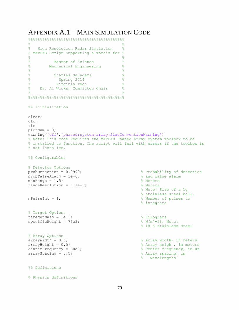
79
APPENDIX A.1 – MAIN SIMULATION CODE %%%%%%%%%%%%%%%%%%%%%%%%%%%%%%%%%%%%%%%%% % % % High Resolution Radar Simulation % % MATLAB Script Supporting a Thesis for % % % % Master of Science % % Mechanical Engineering % % % % Charles Saunders % % Spring 2014 % % Virginia Tech % % Dr. Al Wicks, Committee Chair % % % %%%%%%%%%%%%%%%%%%%%%%%%%%%%%%%%%%%%%%%%%
%% Initialization
clear; clc; tic plotNum = 0; warning('off','phased:system:array:SizeConventionWarning') % Note: This code requires the MATLAB Phased Array System Toolbox to be % installed to function. The script will fail with errors if the toolbox is % not installed.
%% Configurables
% Detector Options probDetection = 0.9999; % Probability of detection probFalseAlarm = 1e-6; % and false alarm maxRange = 1.5; % Meters rangeResolution = 3.1e-3; % Meters % Note: Size of a 1g % stainless steel ball. nPulseInt = 1; % Number of pulses to % integrate
% Target Options taregetMass = 1e-3; % Kilograms specificWeight = 76e3; % N(m^-3), Note: % 18-8 stainless steel
% Array Options arrayWidth = 0.5; % Array width, in meters arrayHeight = 0.5; % Array heigh , in meters centerFrequency = 60e9; % Center frequency, in Hz arraySpacing = 0.5; % Array spacing, in % wavelengths
%% Definitions
% Physics definitions
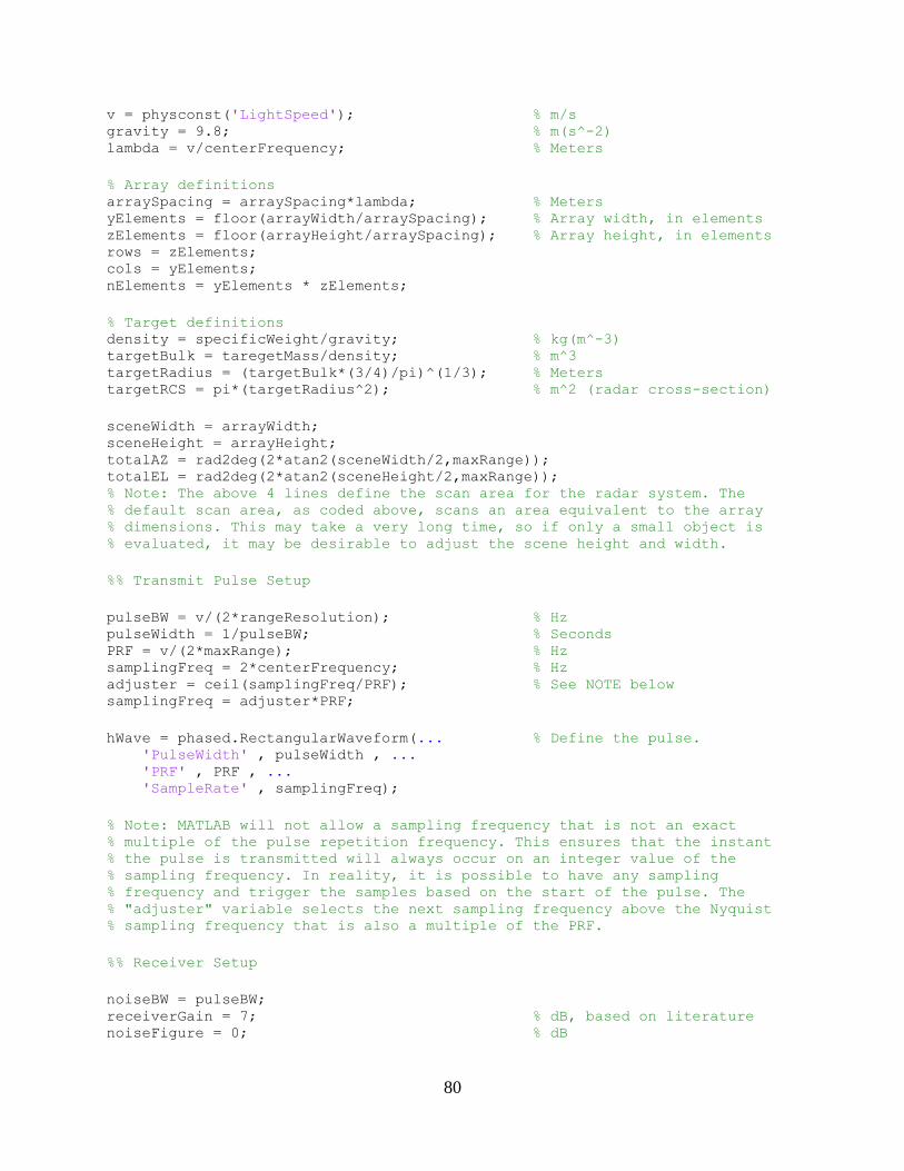
80
v = physconst('LightSpeed'); % m/s gravity = 9.8; % m(s^-2) lambda = v/centerFrequency; % Meters
% Array definitions arraySpacing = arraySpacing*lambda; % Meters yElements = floor(arrayWidth/arraySpacing); % Array width, in elements zElements = floor(arrayHeight/arraySpacing); % Array height, in elements rows = zElements; cols = yElements; nElements = yElements * zElements;
% Target definitions density = specificWeight/gravity; % kg(m^-3) targetBulk = taregetMass/density; % m^3 targetRadius = (targetBulk*(3/4)/pi)^(1/3); % Meters targetRCS = pi*(targetRadius^2); % m^2 (radar cross-section)
sceneWidth = arrayWidth; sceneHeight = arrayHeight; totalAZ = rad2deg(2*atan2(sceneWidth/2,maxRange)); totalEL = rad2deg(2*atan2(sceneHeight/2,maxRange)); % Note: The above 4 lines define the scan area for the radar system. The % default scan area, as coded above, scans an area equivalent to the array % dimensions. This may take a very long time, so if only a small object is % evaluated, it may be desirable to adjust the scene height and width.
%% Transmit Pulse Setup
pulseBW = v/(2*rangeResolution); % Hz pulseWidth = 1/pulseBW; % Seconds PRF = v/(2*maxRange); % Hz samplingFreq = 2*centerFrequency; % Hz adjuster = ceil(samplingFreq/PRF); % See NOTE below samplingFreq = adjuster*PRF;
hWave = phased.RectangularWaveform(... % Define the pulse. 'PulseWidth' , pulseWidth , ... 'PRF' , PRF , ... 'SampleRate' , samplingFreq);
% Note: MATLAB will not allow a sampling frequency that is not an exact % multiple of the pulse repetition frequency. This ensures that the instant % the pulse is transmitted will always occur on an integer value of the % sampling frequency. In reality, it is possible to have any sampling % frequency and trigger the samples based on the start of the pulse. The % "adjuster" variable selects the next sampling frequency above the Nyquist % sampling frequency that is also a multiple of the PRF.
%% Receiver Setup
noiseBW = pulseBW; receiverGain = 7; % dB, based on literature noiseFigure = 0; % dB
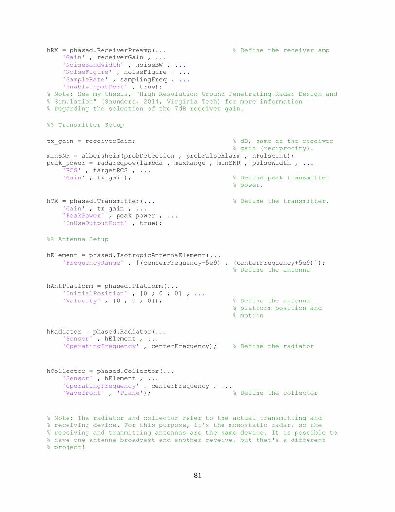
81
hRX = phased.ReceiverPreamp(... % Define the receiver amp 'Gain' , receiverGain , ... 'NoiseBandwidth' , noiseBW , ... 'NoiseFigure' , noiseFigure , ... 'SampleRate' , samplingFreq , ... 'EnableInputPort' , true); % Note: See my thesis, "High Resolution Ground Penetrating Radar Design and % Simulation" (Saunders, 2014, Virginia Tech) for more information % regarding the selection of the 7dB receiver gain.
%% Transmitter Setup
tx_gain = receiverGain; % dB, same as the receiver % gain (reciprocity). minSNR = albersheim(probDetection , probFalseAlarm , nPulseInt); peak_power = radareqpow(lambda , maxRange , minSNR , pulseWidth , ... 'RCS' , targetRCS , ... 'Gain' , tx_gain); % Define peak transmitter % power.
hTX = phased.Transmitter(... % Define the transmitter. 'Gain' , tx_gain , ... 'PeakPower' , peak_power , ... 'InUseOutputPort' , true);
%% Antenna Setup
hElement = phased.IsotropicAntennaElement(... 'FrequencyRange' , [(centerFrequency-5e9) , (centerFrequency+5e9)]); % Define the antenna
hAntPlatform = phased.Platform(... 'InitialPosition' , [0 ; 0 ; 0] , ... 'Velocity' , [0 ; 0 ; 0]); % Define the antenna % platform position and % motion
hRadiator = phased.Radiator(... 'Sensor' , hElement , ... 'OperatingFrequency' , centerFrequency); % Define the radiator
hCollector = phased.Collector(... 'Sensor' , hElement , ... 'OperatingFrequency' , centerFrequency , ... 'Wavefront' , 'Plane'); % Define the collector
% Note: The radiator and collector refer to the actual transmitting and % receiving device. For this purpose, it's the monostatic radar, so the % receiving and tranmitting antennas are the same device. It is possible to % have one antenna broadcast and another receive, but that's a different % project!
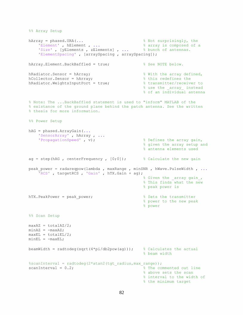
82
%% Array Setup
hArray = phased.URA(... % Not surprisingly, the 'Element' , hElement , ... % array is composed of a 'Size' , [yElements , zElements] , ... % bunch of antennas. 'ElementSpacing' , [arraySpacing , arraySpacing]);
hArray.Element.BackBaffled = true; % See NOTE below.
hRadiator.Sensor = hArray; % With the array defined, hCollector.Sensor = hArray; % this redefines the hRadiator.WeightsInputPort = true; % transmitter/receiver to % use the _array_ instead % of an individual antenna
% Note: The ...BackBaffled statement is used to "inform" MATLAB of the % existance of the ground plane behind the patch antenna. See the written % thesis for more information.
%% Power Setup
hAG = phased.ArrayGain(... 'SensorArray' , hArray , ... 'PropagationSpeed' , v); % Defines the array gain, % given the array setup and % antenna elements used
ag = step(hAG , centerFrequency , [0;0]); % Calculate the new gain
peak_power = radareqpow(lambda , maxRange , minSNR , hWave.PulseWidth , ... 'RCS' , targetRCS , 'Gain' , hTX.Gain + ag); % Given the _array gain_, % This finds what the new % peak power is
hTX.PeakPower = peak_power; % Sets the transmitter % power to the new peak % power
%% Scan Setup
maxAZ = totalAZ/2; minAZ = -maxAZ; maxEL = totalEL/2; minEL = -maxEL;
beamWidth = radtodeg(sqrt(4*pi/db2pow(ag))); % Calculates the actual % beam width
%scanInterval = radtodeg(2*atan2(tgt_radius,max_range)); scanInterval = 0.2; % The commented out line % above sets the scan % interval to the width of % the minimum target
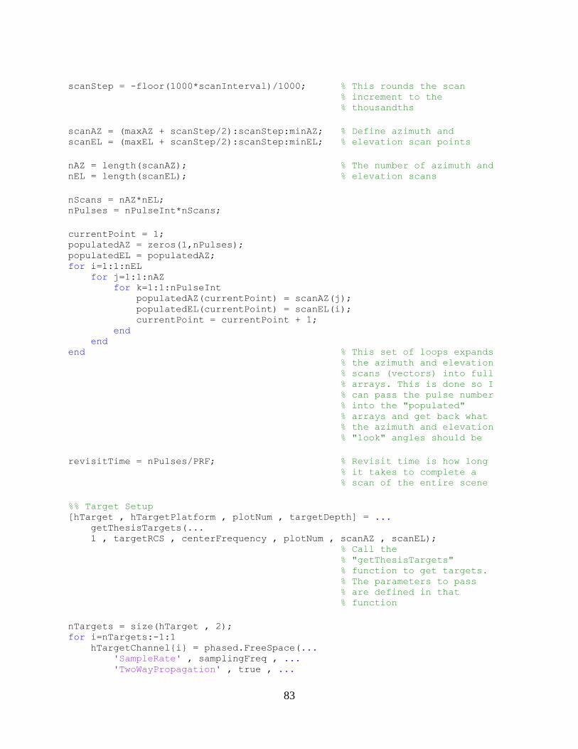
83
scanStep = -floor(1000*scanInterval)/1000; % This rounds the scan % increment to the % thousandths
scanAZ = (maxAZ + scanStep/2):scanStep:minAZ; % Define azimuth and scanEL = (maxEL + scanStep/2):scanStep:minEL; % elevation scan points
nAZ = length(scanAZ); % The number of azimuth and nEL = length(scanEL); % elevation scans
nScans = nAZ*nEL; nPulses = nPulseInt*nScans;
currentPoint = 1; populatedAZ = zeros(1,nPulses); populatedEL = populatedAZ; for i=1:1:nEL for j=1:1:nAZ for k=1:1:nPulseInt populatedAZ(currentPoint) = scanAZ(j); populatedEL(currentPoint) = scanEL(i); currentPoint = currentPoint + 1; end end end % This set of loops expands % the azimuth and elevation % scans (vectors) into full % arrays. This is done so I % can pass the pulse number % into the "populated" % arrays and get back what % the azimuth and elevation % "look" angles should be
revisitTime = nPulses/PRF; % Revisit time is how long % it takes to complete a % scan of the entire scene
%% Target Setup [hTarget , hTargetPlatform , plotNum , targetDepth] = ... getThesisTargets(... 1 , targetRCS , centerFrequency , plotNum , scanAZ , scanEL); % Call the % "getThesisTargets" % function to get targets. % The parameters to pass % are defined in that % function
nTargets = size(hTarget , 2); for i=nTargets:-1:1 hTargetChannel{i} = phased.FreeSpace(... 'SampleRate' , samplingFreq , ... 'TwoWayPropagation' , true , ...
84
'OperatingFrequency' , centerFrequency); end % Get the number of targets % and then define that the % wave must propagate in % two directions for each % target.
%% Beamformer Setup
hSV = phased.SteeringVector(... % The array (hArray) is to 'SensorArray' , hArray , ... % be steered. . . 'PropagationSpeed' , v);
hBF = phased.PhaseShiftBeamformer(... % . . . using the phase 'SensorArray' , hArray , ... % shift beamformer. 'OperatingFrequency' , centerFrequency , ... 'PropagationSpeed' , v , ... 'DirectionSource' , 'Input port');
%% Pre-simulation Memory Allocation/Setup
% The simulations for a 0.5 wavelength grid spacing take a LONG time, even % on a small array. This preallocates the variables needed for % post-processing to ensure that you don't have to wait forever for the % simulations to run, only to run out of memory when the data is processed. % I could not simulate the full array with 4GB of RAM. I purchased 16GB of % RAM to complete the simulations.
fastTimeGrid = unigrid(0 , 1/samplingFreq , 1/PRF , '[)'); % FastTimeGrid is the time % grid at the sampling % frequency that occurs % during the pulse. targetAngle = zeros(2,nTargets);
% A note briefly about the System Objects used by the Phased Array System % Toolbox. The "step( )" function is what "uses" or "activates" the System % Object. Below, "step(hWave)" is what actually generates the wave form. % The earlier definition of hWave simply defined the parameters that would % dictate the wave. wave = step(hWave);
% Similarly, "step(hTX, wave)" causes the transmitter, defined by the hTX % definition earlier, to actually transmit the wave that was just % generated. [signal , tx_status] = step(hTX , wave);
% "step(hAntPlatform , 1/PRF)" calculates the new position and velocity of % the array platform given the amount of time between pulses (1/PRF). [ant_pos , ant_vel] = step(hAntPlatform , 1/PRF);
% The antenna platform may move, and the targets can move also. This % updates the speed and cartesian (absolute) and polar (relative) locations % of each of the targets. for i = nTargets:-1:1

85
[tgt_pos(:,i) , tgt_vel(:,i)] = step(hTargetPlatform{i} , 1/PRF); [~ , targetAngle(:,i)] = rangeangle(tgt_pos(:,i) , ant_pos); end
rxAZ = zeros(1,nScans); rxEL = rxAZ; % rxAZ and rxEL provide a % place to log whether or % not an object was % detected. These points % align with the points in % the "populatedAX" and EL % variables defined % earlier.
nDataPoints = length(signal); rxPulses = zeros(nDataPoints , nPulses); receivedSignal = zeros(nDataPoints , nTargets); % The above variables represent how the signal is handled. nDataPoints is % the number of points in the transmitted wave. The wave will bounce off of % each target, so the "receivedSignal" has to be nDataPoints by nTargets. % Related, but different, is the received _pulses_, "rxPulses". Each % received PULSE is comprised of the SUMMATION of all of the received % signals. Each received signal is nDataPointsLong, so rxPulses is % nDataPoints long, but it's the processed result for each pulses, so it's % nDataPoints by nPulses.
MFIntermediatePulses = rxPulses; MFPulses = zeros(nDataPoints , nPulseInt , nScans); TVGPulses = MFPulses; intPulses = zeros(nDataPoints , nScans); % The above variables are for intermediate signal processing. This is where % you can quickly run out of memory. These values, as initialized, aren't % used as they are generated as the result of a function. However, if you % wait until calling the function to allocate the memory, you could crash % the program after waiting for the simulations to run.
pulseNotify = ceil(nPulses/100); fprintf('Working...') fprintf('nPulses is %d' , nPulses) % The above is a text tracker to help monitor the simulation process. % Simulations of one small object and a restricted scene usually take ten % minutes to an hour, and simulations of the full sene with many objects % take days to over a week to run.
% The loop below is what actually simulates the radar system for i = 1:nPulses
if mod(i,pulseNotify)==0 clc; elapsed = toc; fprintf('Currently %d percent complete\n', (i/pulseNotify)) fprintf('Elapsed time is %d seconds\n' , floor(elapsed)) fprintf('Estimated time remaining is %d seconds\n' , ... floor((100*elapsed/(i/pulseNotify)) - elapsed)) fprintf('Estimated total time is %d seconds' , ... floor(100*elapsed/(i/pulseNotify)))
86
end % The above code looks at the time that has passed since the simulation % started, and what percentage it thinks it has completed, and % generates an estimate of how long it thinks it will take to complete % the simulations.
azimuth = populatedAZ(i); % Get the current azimuth elevation = populatedEL(i); % and elevation to scan
scanVector = step(hSV , centerFrequency , [azimuth ; elevation]); weights = conj(scanVector); % Setup the phase shift
for j = nTargets:-1:1 % For each target. . .
targetSignal = step(hRadiator , ... signal , targetAngle(:,j) , weights); % . . . transmit the % signal. . .
targetSignal = step(... % . . . then have that hTargetChannel{j} , ... % signal propagate. . . targetSignal , ant_pos , ... tgt_pos(:,j) , ant_vel , ... tgt_vel(:,j));
receivedSignal(:,j) = step(... % . . . then have that hTarget{j} , targetSignal); % "bounce" off the target. end
receivedSignal = step(hCollector , receivedSignal , targetAngle); % Collect all received % signals. . . receivedSignal = step(hRX , receivedSignal , ~(tx_status>0)); % . . . amplify them. . . receivedSignal = step(hBF , receivedSignal , [azimuth; elevation]); % . . . apply the % beamformer . . . rxPulses(:,i) = receivedSignal; % . . . and record the % received pulse. end
% I hope the end of this loop helps clarify what I had talked about in the % previous section. The received signal is exists for every target. When % the hCollector System Object is called, those multiple signals are % "collapsed" into one signal - the returned pulse. There is some basic % initial processing (amplification and beamforming) that is performed % before the received wave is recorded. Post-processing occurs next.
%% Signal Processing
initialAz = maxAZ; endAz = minAZ;
matchingCoeff = getMatchedFilter(hWave);

87
hMF = phased.MatchedFilter(... 'Coefficients' , matchingCoeff , ... 'GainOutputPort' , true); [MFIntermediatePulses , MF_gain] = step(hMF , rxPulses); MFPulses = reshape(MFIntermediatePulses , [] , nPulseInt , nScans); matchingDelay = size(matchingCoeff , 1) - 1; nMFPulses = size(MFPulses); MFPulses = [MFPulses((matchingDelay + 1):end) , ... zeros(1 , matchingDelay)]; MFPulses = reshape(MFPulses , nMFPulses); % The above code applies a matched filter to the data. See the thesis for a % more involved discussion, but briefly, the matched filter convolves the % data with a mirrored conjugated version of the transmitted pulse.
rangeGates = v*fastTimeGrid/2; % Range gates are just how % far the wave could move % in a given time % increment. Here it's % determined by the % fastTimeGrid, which % again, is the sampling % frequency periods for the % duration of a pulse at % maximum operating range. hTVG = phased.TimeVaryingGain(... 'RangeLoss' , 2*fspl(rangeGates , lambda) , ... 'ReferenceLoss' , 2*fspl(max(rangeGates) , lambda)); TVGPulses = step(hTVG , MFPulses); % Again, see the thesis for a discussion of time varying gain. The code % above applies the time varying gain.
intPulses = pulsint(TVGPulses , 'noncoherent'); intPulses = squeeze(intPulses); % The code above performs the pulse integration.
noise_power = noisepow(hRX.NoiseBandwidth , ... hRX.NoiseFigure , hRX.ReferenceTemperature); threshold = noise_power * db2pow(... npwgnthresh(probFalseAlarm , nPulseInt , 'noncoherent')); threshold = threshold * db2pow(MF_gain); % The code above finds the signal magnitude threshold for a valid response.
[I,J] = find(abs(intPulses).^2 > threshold); % Anywhere the magnitude of % a pulse is above the % threshold, record it as a % valid response. currentPoint = 1; for i = 1:length(scanEL) for j = 1:length(scanAZ) rxAZ(currentPoint) = populatedAZ( (currentPoint-1)*nPulseInt + 1); rxEL(currentPoint) = populatedEL( (currentPoint-1)*nPulseInt + 1); currentPoint = currentPoint + 1; end end
88
estRange = rangeGates(I); % Estimated range estAZ = rxAZ(J); % Estimated direction estEL = rxEL(J);
%% Output Text
fprintf('Scan interval is: % 7.4f\n' , scanInterval) fprintf('Actual beam width is: % 7.4f\n' , beamWidth) fprintf('The revisit time is: % 7.4f s, or % 7.4f ms\n' , ... revisitTime , 1000*revisitTime) % Display some facts about % the scan
for i=1:1:2 % Generate output plots!
plotNum = plotNum + 1; dataPlotter(estAZ , estEL , estRange , scanStep , plotNum) if i==2 gridPlot(scanAZ,scanEL,targetDepth) end % dataPlotter and gridPlot % are both custom functions axis equal axis([0 1.5 -0.25 0.25 -0.25 0.25]) view([-90,0]) hold off end
% As a final note, any custom functions (dataPlotter, gridPlot, and % getThesisTargets) are all disclosed in Appendix A of my thesis.
89
APPENDIX A.2 – TARGET FETCHING CODE function [hTarget , hTargetPlatform , plotNum , targetDepth] = ... getThesisTargets(style , tgt_rcs , fc , plotNum , scanAZ , scanEL) % This cleans up my code significantly by hiding the (ugly) chunk of code % that sets the targets. Pass a shape in, get targets out. % % The function is called % [hTarget , hTargetPlatform , plotNum , targetDepth] = % getThesisTargets(style , tgt_rcs , fc , plotNum , scanAZ , scanEL) % % where the inputs are defined as: % style: A numeric value, 1-6, that defines the shape of the targets % 1 = Three small targets % 2 = Smiley face % 3 = [deleted] % 4 = One small target % 5 = Several targets, in a line, of various sizes % 6 = The crowded scene % tgt_rcs: The radar cross-section of the minimum target. % fc: The center frequency of the radar system. % plotNum: The current plot number % scanAZ: The azimuth scan vector % scanEL: The elevation scan vector % % and the outputs are: % hTarget: The System Object defining all targets % hTargetPlatform: The System Object defining the platform for all % targets % plotNum: The current plot number (after making plots) % targetDepth: The depth of the targets (used for making grid % overlays) % There are no significant comments throughout the remainder of the code; % see the thesis for more information.
sphereRes = 10; targetDepth = 1.3;
switch style case 1 % Three small targets targets = [ [1.3 ; 0 ; 0] , ... % [x;y;z] position in [1.3 ; 0.01608 ; 0] , ... % meters [1.3 ; -0.01608 ; 0]]; targetDepth = 1.3; nTargets = size(targets,2); plotR = [0.003,0.003,0.003]; hTarget{1} = phased.RadarTarget(... 'MeanRCS' , tgt_rcs , ... 'OperatingFrequency' , fc); hTargetPlatform{1} = phased.Platform(... 'InitialPosition' , targets(:,1) , ... 'Velocity' , [0; 0; 0]);
if nTargets>1 for i=nTargets:-1:2 hTarget{i} = phased.RadarTarget(...

90
'MeanRCS' , tgt_rcs , ... 'OperatingFrequency' , fc); hTargetPlatform{i} = phased.Platform(... 'InitialPosition' , targets(:,i) , ... 'Velocity' , [0; 0; 0]); end end
case 2 % Smiley face theta = 0:(pi/10):2*pi; r = 0.08;
targetDepth = 1.1;
faceY = r*cos(theta); faceZ = r*sin(theta); faceX = targetDepth * ones(1,length(faceY)); faceTargets = [faceX; faceY; faceZ];
smileTheta = 0:(pi/5):pi; smileR = r/2; smileY = 1.2*smileR*cos(smileTheta); smileZ = -1.2*smileR*sin(smileTheta); smileX = targetDepth * ones(1,length(smileY)); smileTargets = [smileX; smileY; smileZ];
eyes = [[targetDepth; -0.8*smileR; 0.8*smileR],... [targetDepth; 0.8*smileR; 0.8*smileR]];
nose = [[targetDepth; 0; smileR-0.5*smileR],... [targetDepth-(smileR/2); 0; (smileR/2)-0.5*smileR],... [targetDepth-(smileR); 0; 0-0.5*smileR],... [targetDepth; 0; 0-0.5*smileR]]; targets = [faceTargets , smileTargets , eyes , nose];
for i=size(targets,2):-1:1 hTarget{i} = phased.RadarTarget(... 'MeanRCS' , tgt_rcs , ... 'OperatingFrequency' , fc); hTargetPlatform{i} = phased.Platform(... 'InitialPosition' , targets(:,i) , ... 'Velocity' , [0; 0; 0]); end
case 3 % Three large objects % Removed, superceded by Case 5.
case 4 % Single small object
targetDepth = 1.4;
%tgt_radius = sqrt(tgt_rcs/pi); %tgt_multiplier = 2;
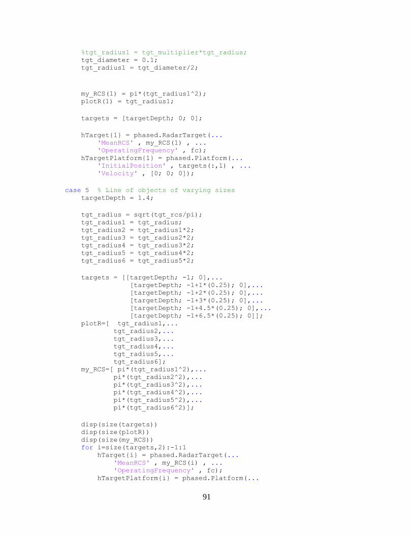
91
%tgt_radius1 = tgt_multiplier*tgt_radius; tgt_diameter = 0.1; tgt_radius1 = tgt_diameter/2;
my_RCS(1) = pi*(tgt_radius1^2); plotR(1) = tgt_radius1;
targets = [targetDepth; 0; 0];
hTarget{1} = phased.RadarTarget(... 'MeanRCS' , my_RCS(1) , ... 'OperatingFrequency' , fc); hTargetPlatform{1} = phased.Platform(... 'InitialPosition' , targets(:,1) , ... 'Velocity' , [0; 0; 0]);
case 5 % Line of objects of varying sizes targetDepth = 1.4;
tgt_radius = sqrt(tgt_rcs/pi); tgt_radius1 = tgt_radius; tgt_radius2 = tgt_radius1*2; tgt_radius3 = tgt_radius2*2; tgt_radius4 = tgt_radius3*2; tgt_radius5 = tgt_radius4*2; tgt_radius6 = tgt_radius5*2;
targets = [[targetDepth; -1; 0],... [targetDepth; -1+1*(0.25); 0],... [targetDepth; -1+2*(0.25); 0],... [targetDepth; -1+3*(0.25); 0],... [targetDepth; -1+4.5*(0.25); 0],... [targetDepth; -1+6.5*(0.25); 0]]; plotR=[ tgt_radius1,... tgt_radius2,... tgt_radius3,... tgt_radius4,... tgt_radius5,... tgt_radius6]; my_RCS=[ pi*(tgt_radius1^2),... pi*(tgt_radius2^2),... pi*(tgt_radius3^2),... pi*(tgt_radius4^2),... pi*(tgt_radius5^2),... pi*(tgt_radius6^2)];
disp(size(targets)) disp(size(plotR)) disp(size(my_RCS)) for i=size(targets,2):-1:1 hTarget{i} = phased.RadarTarget(... 'MeanRCS' , my_RCS(i) , ... 'OperatingFrequency' , fc); hTargetPlatform{i} = phased.Platform(...
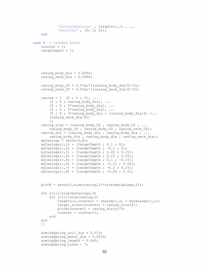
92
'InitialPosition' , targets(:,i) , ... 'Velocity' , [0; 0; 0]); end
case 6 % Crowded scene counter = 1; targetDepth = 1;
casing_body_dia = 0.0095; casing_neck_dia = 0.0064;
casing_body_CS = 0.5*pi*((casing_body_dia/2)^2); casing_neck_CS = 0.5*pi*((casing_neck_dia/2)^2);
casing = [ [0 ; 0 ; 0], ... [0 ; 0 ; casing_body_dia], ... [0 ; 0 ; 2*casing_body_dia], ... [0 ; 0 ; 3*casing_body_dia], ... [0 ; 0 ; 3*casing_body_dia + (casing_body_dia/2) +... (casing_neck_dia/2)] ]; casing_size = [casing_body_CS , casing_body_CS , ... casing_body_CS , casing_body_CS , casing_neck_CS]; casing_dia = [casing_body_dia , casing_body_dia , ... casing_body_dia , casing_body_dia , casing_neck_dia]; myCasings = zeros(3,8); myCasings(:,1) = [targetDepth ; 0.1 ; 0]; myCasings(:,2) = [targetDepth ; -0.1 ; 0]; myCasings(:,3) = [targetDepth ; 0.05 ; 0.15]; myCasings(:,4) = [targetDepth ; 0.15 ; 0.15]; myCasings(:,5) = [targetDepth ; 0.1 ; -0.15]; myCasings(:,6) = [targetDepth ; -0.15 ; 0.05]; myCasings(:,7) = [targetDepth ; -0.2 ; 0.15]; myCasings(:,8) = [targetDepth ; -0.05 ; 0.2];
plotR = zeros(1,size(casing,2)*size(myCasings,2));
for i=1:1:size(myCasings,2) for j=1:1:size(casing,2) targets(:,counter) = casing(:,j) + myCasings(:,i); target_sizes(counter) = casing_size(j); plotR(counter) = casing_dia(j)/2; counter = counter+1; end end %}
armingSpring_coil_dia = 0.015; armingSpring_metal_dia = 0.0016; armingSpring_length = 0.040; armingSpring_turns = 7;
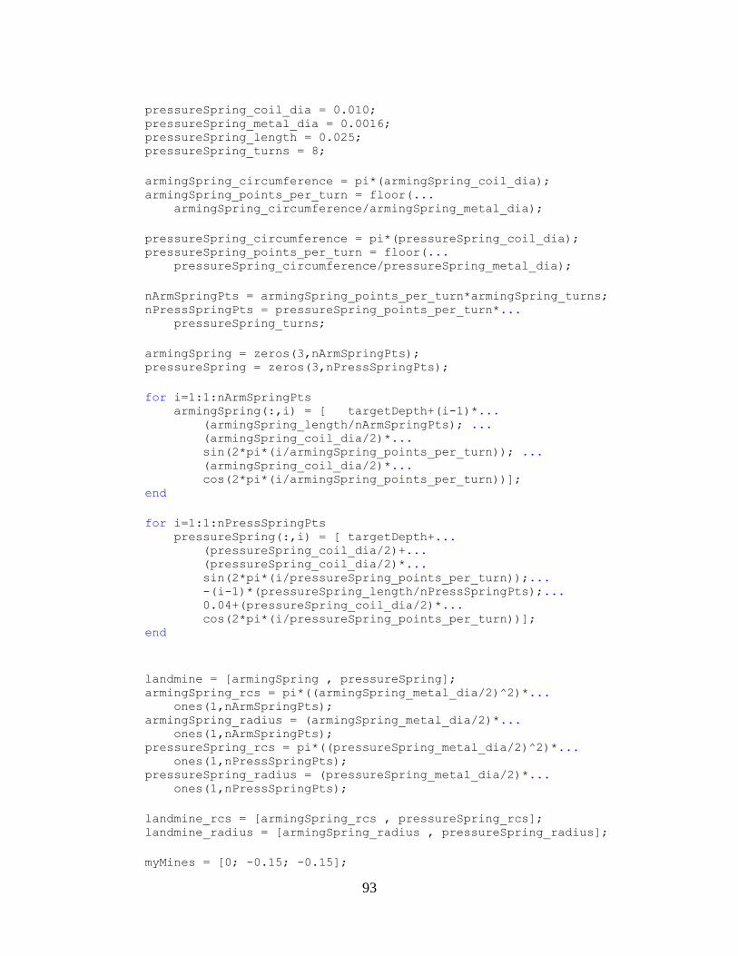
93
pressureSpring_coil_dia = 0.010; pressureSpring_metal_dia = 0.0016; pressureSpring_length = 0.025; pressureSpring_turns = 8;
armingSpring_circumference = pi*(armingSpring_coil_dia); armingSpring_points_per_turn = floor(... armingSpring_circumference/armingSpring_metal_dia);
pressureSpring_circumference = pi*(pressureSpring_coil_dia); pressureSpring_points_per_turn = floor(... pressureSpring_circumference/pressureSpring_metal_dia);
nArmSpringPts = armingSpring_points_per_turn*armingSpring_turns; nPressSpringPts = pressureSpring_points_per_turn*... pressureSpring_turns;
armingSpring = zeros(3,nArmSpringPts); pressureSpring = zeros(3,nPressSpringPts);
for i=1:1:nArmSpringPts armingSpring(:,i) = [ targetDepth+(i-1)*... (armingSpring_length/nArmSpringPts); ... (armingSpring_coil_dia/2)*... sin(2*pi*(i/armingSpring_points_per_turn)); ... (armingSpring_coil_dia/2)*... cos(2*pi*(i/armingSpring_points_per_turn))]; end
for i=1:1:nPressSpringPts pressureSpring(:,i) = [ targetDepth+... (pressureSpring_coil_dia/2)+... (pressureSpring_coil_dia/2)*... sin(2*pi*(i/pressureSpring_points_per_turn));... -(i-1)*(pressureSpring_length/nPressSpringPts);... 0.04+(pressureSpring_coil_dia/2)*... cos(2*pi*(i/pressureSpring_points_per_turn))]; end
landmine = [armingSpring , pressureSpring]; armingSpring_rcs = pi*((armingSpring_metal_dia/2)^2)*... ones(1,nArmSpringPts); armingSpring_radius = (armingSpring_metal_dia/2)*... ones(1,nArmSpringPts); pressureSpring_rcs = pi*((pressureSpring_metal_dia/2)^2)*... ones(1,nPressSpringPts); pressureSpring_radius = (pressureSpring_metal_dia/2)*... ones(1,nPressSpringPts);
landmine_rcs = [armingSpring_rcs , pressureSpring_rcs]; landmine_radius = [armingSpring_radius , pressureSpring_radius];
myMines = [0; -0.15; -0.15];
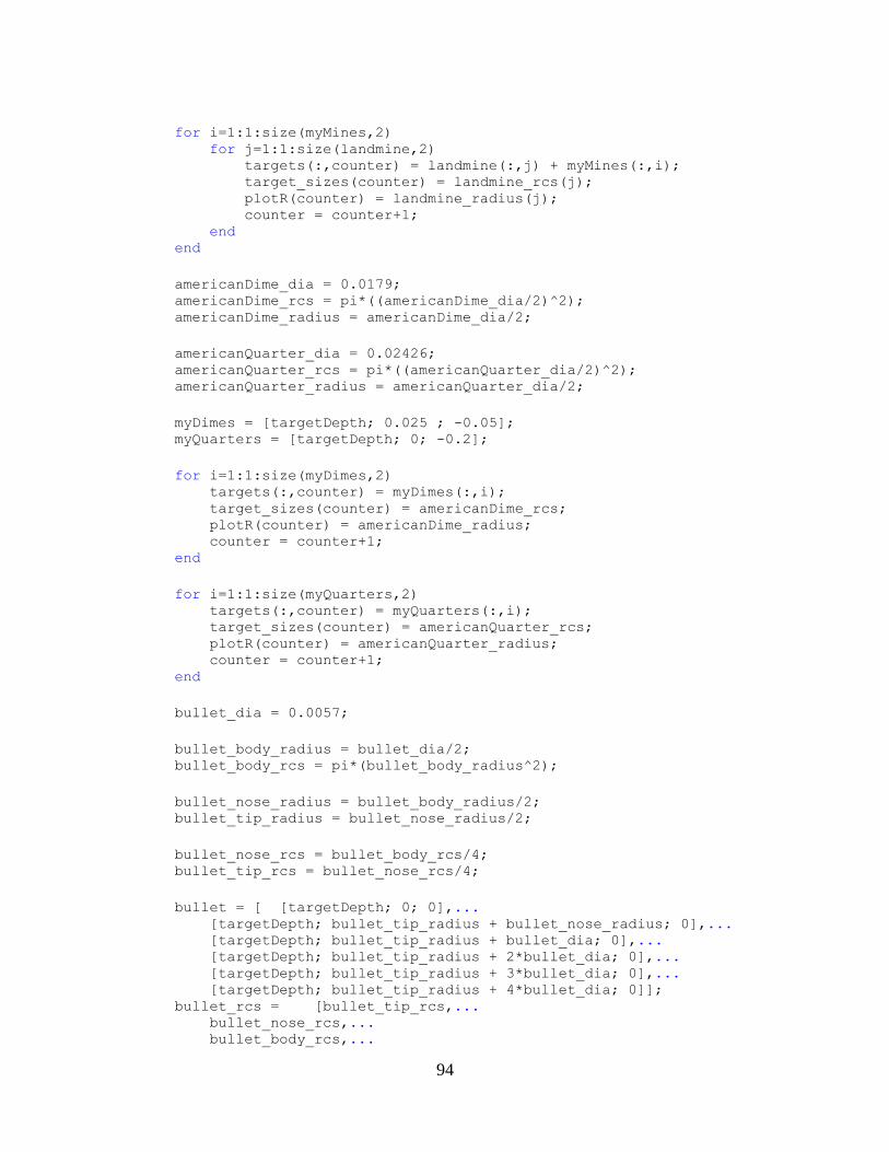
94
for i=1:1:size(myMines,2) for j=1:1:size(landmine,2) targets(:,counter) = landmine(:,j) + myMines(:,i); target_sizes(counter) = landmine_rcs(j); plotR(counter) = landmine_radius(j); counter = counter+1; end end
americanDime_dia = 0.0179; americanDime_rcs = pi*((americanDime_dia/2)^2); americanDime_radius = americanDime_dia/2;
americanQuarter_dia = 0.02426; americanQuarter_rcs = pi*((americanQuarter_dia/2)^2); americanQuarter_radius = americanQuarter_dia/2;
myDimes = [targetDepth; 0.025 ; -0.05]; myQuarters = [targetDepth; 0; -0.2];
for i=1:1:size(myDimes,2) targets(:,counter) = myDimes(:,i); target_sizes(counter) = americanDime_rcs; plotR(counter) = americanDime_radius; counter = counter+1; end
for i=1:1:size(myQuarters,2) targets(:,counter) = myQuarters(:,i); target_sizes(counter) = americanQuarter_rcs; plotR(counter) = americanQuarter_radius; counter = counter+1; end
bullet_dia = 0.0057;
bullet_body_radius = bullet_dia/2; bullet_body_rcs = pi*(bullet_body_radius^2);
bullet_nose_radius = bullet_body_radius/2; bullet_tip_radius = bullet_nose_radius/2;
bullet_nose_rcs = bullet_body_rcs/4; bullet_tip_rcs = bullet_nose_rcs/4;
bullet = [ [targetDepth; 0; 0],... [targetDepth; bullet_tip_radius + bullet_nose_radius; 0],... [targetDepth; bullet_tip_radius + bullet_dia; 0],... [targetDepth; bullet_tip_radius + 2*bullet_dia; 0],... [targetDepth; bullet_tip_radius + 3*bullet_dia; 0],... [targetDepth; bullet_tip_radius + 4*bullet_dia; 0]]; bullet_rcs = [bullet_tip_rcs,... bullet_nose_rcs,... bullet_body_rcs,...
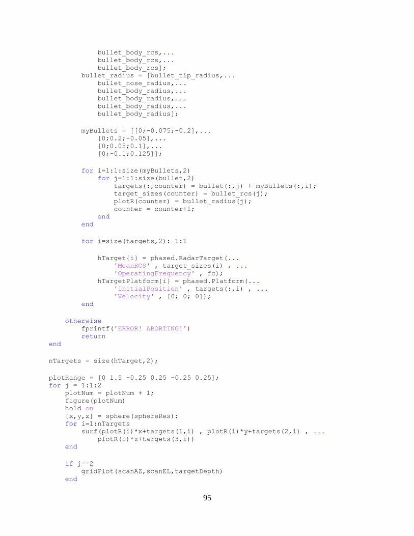
95
bullet_body_rcs,... bullet_body_rcs,... bullet_body_rcs]; bullet_radius = [bullet_tip_radius,... bullet_nose_radius,... bullet_body_radius,... bullet_body_radius,... bullet_body_radius,... bullet_body_radius];
myBullets = [[0;-0.075;-0.2],... [0;0.2;-0.05],... [0;0.05;0.1],... [0;-0.1;0.125]];
for i=1:1:size(myBullets,2) for j=1:1:size(bullet,2) targets(:,counter) = bullet(:,j) + myBullets(:,i); target_sizes(counter) = bullet_rcs(j); plotR(counter) = bullet_radius(j); counter = counter+1; end end
for i=size(targets,2):-1:1
hTarget{i} = phased.RadarTarget(... 'MeanRCS' , target_sizes(i) , ... 'OperatingFrequency' , fc); hTargetPlatform{i} = phased.Platform(... 'InitialPosition' , targets(:,i) , ... 'Velocity' , [0; 0; 0]); end
otherwise fprintf('ERROR! ABORTING!') return end
nTargets = size(hTarget,2);
plotRange = [0 1.5 -0.25 0.25 -0.25 0.25]; for j = 1:1:2 plotNum = plotNum + 1; figure(plotNum) hold on [x,y,z] = sphere(sphereRes); for i=1:nTargets surf(plotR(i)*x+targets(1,i) , plotR(i)*y+targets(2,i) , ... plotR(i)*z+targets(3,i)) end
if j==2 gridPlot(scanAZ,scanEL,targetDepth) end

96
axis equal axis(plotRange) view([-90,0]) hold off end
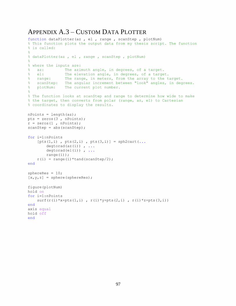
97
APPENDIX A.3 – CUSTOM DATA PLOTTER function dataPlotter(az , el , range , scanStep , plotNum) % This function plots the output data from my thesis script. The function % is called: % % dataPlotter(az , el , range , scanStep , plotNum) % % where the inputs are: % az: The azimuth angle, in degrees, of a target. % el: The elevation angle, in degrees, of a target. % range: The range, in meters, from the array to the target. % scanStep: The angular increment between "look" angles, in degrees. % plotNum: The current plot number. % % The function looks at scanStep and range to determine how wide to make % the target, then converts from polar (range, az, el) to Cartesian % coordinates to display the results.
nPoints = length(az); pts = zeros(3 , nPoints); r = zeros(1 , nPoints); scanStep = abs(scanStep);
for i=1:nPoints [pts(1,i) , pts(2,i) , pts(3,i)] = sph2cart(... degtorad(az(i)) , ... degtorad(el(i)) , ... range(i)); r(i) = range(i)*tand(scanStep/2); end
sphereRes = 10; [x,y,z] = sphere(sphereRes);
figure(plotNum) hold on for i=1:nPoints surf(r(i)*x+pts(1,i) , r(i)*y+pts(2,i) , r(i)*z+pts(3,i)) end axis equal hold off end
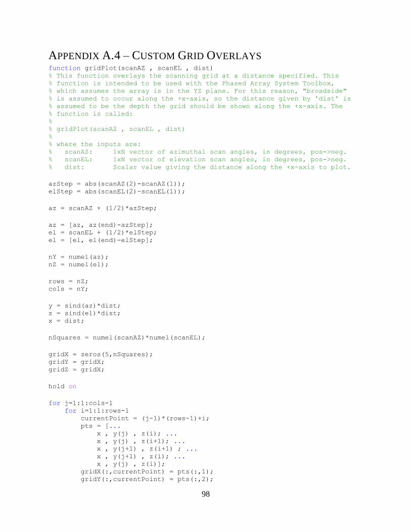
98
APPENDIX A.4 – CUSTOM GRID OVERLAYS function gridPlot(scanAZ , scanEL , dist) % This function overlays the scanning grid at a distance specified. This % function is intended to be used with the Phased Array System Toolbox, % which assumes the array is in the YZ plane. For this reason, "broadside" % is assumed to occur along the +x-axis, so the distance given by 'dist' is % assumed to be the depth the grid should be shown along the +x-axis. The % function is called: % % gridPlot(scanAZ , scanEL , dist) % % where the inputs are: % scanAZ: 1xN vector of azimuthal scan angles, in degrees, pos->neg. % scanEL: 1xN vector of elevation scan angles, in degrees, pos->neg. % dist: Scalar value giving the distance along the +x-axis to plot.
azStep = abs(scanAZ(2)-scanAZ(1)); elStep = abs(scanEL(2)-scanEL(1));
az = scanAZ + (1/2)*azStep;
az = [az, az(end)-azStep]; el = scanEL + (1/2)*elStep; el = [el, el(end)-elStep];
nY = numel(az); nZ = numel(el);
rows = nZ; cols = nY;
y = sind(az)*dist; z = sind(el)*dist; x = dist;
nSquares = numel(scanAZ)*numel(scanEL);
gridX = zeros(5,nSquares); gridY = gridX; gridZ = gridX;
hold on
for j=1:1:cols-1 for i=1:1:rows-1 currentPoint = (j-1)*(rows-1)+i; pts = [... x , y(j) , z(i); ... x , y(j) , z(i+1); ... x , y(j+1) , z(i+1) ; ... x , y(j+1) , z(i); ... x , y(j) , z(i)]; gridX(:,currentPoint) = pts(:,1); gridY(:,currentPoint) = pts(:,2);

99
gridZ(:,currentPoint) = pts(:,3); plot3(gridX(:,currentPoint),gridY(:,currentPoint),... gridZ(:,currentPoint)) end end fprintf('Azimuthal grid spacing is % 5.2E m\n' , abs(y(2)-y(1))) fprintf('Elevation grid spacing is % 5.2E m\n' , abs(z(2)-z(1))) hold off end