High-Precision Robot Odometry Using an

Array of Optical MiceSteven Bell Student Member, IEEE

Oklahoma Christian University

24 March 2011

2

ACKNOWLEDGEMENTS

I am grateful for Dr. David Waldo’s guidance during this project and for his support of the Oklahoma Christian

IEEE student branch, and to Dr. Bill Ryan for his help in the manufacturing aspects of this work. I would also like

to thank Avago Technologies, Marshall Electronics, and M12 Lenses, Inc, for supplying free and discounted parts

for this project.

CONTENTS

I Introduction 3

I-A Prior research . . . . . . . . . . . . . . . . . . . . . . . . . . . . . . . . . . . . . . . . . . . 3

I-B Conditions for mouse use . . . . . . . . . . . . . . . . . . . . . . . . . . . . . . . . . . . . . 4

II Sensor design 5

II-A Hardware design . . . . . . . . . . . . . . . . . . . . . . . . . . . . . . . . . . . . . . . . . . 5

II-B Software driver . . . . . . . . . . . . . . . . . . . . . . . . . . . . . . . . . . . . . . . . . . 7

III Motion tracking 7

IV Error reduction 11

IV-A Integration of multiple sensors . . . . . . . . . . . . . . . . . . . . . . . . . . . . . . . . . . 11

IV-B Use of encoder data . . . . . . . . . . . . . . . . . . . . . . . . . . . . . . . . . . . . . . . . 11

IV-C Use of surface quality . . . . . . . . . . . . . . . . . . . . . . . . . . . . . . . . . . . . . . . 12

V Additional uses 12

VI Conclusions and Future work 13

References 13

Appendix 15

A Optical mouse theory of operation . . . . . . . . . . . . . . . . . . . . . . . . . . . . . . . . 15

B Lens comparison and selection . . . . . . . . . . . . . . . . . . . . . . . . . . . . . . . . . . 15

C Mouse motion simulations . . . . . . . . . . . . . . . . . . . . . . . . . . . . . . . . . . . . 17

3

Abstract

This paper describes a robot position tracking system based on a set of six optical mice. Each mouse sensor uses

a lens which results in higher tracking speeds and allows the sensor to be placed centimeters, rather than millimeters,

from the floor. The sensors’ tracking and data reporting characteristics are discussed, and an algorithm is presented

to determine a robot’s motion from the sensor readings. Techniques for error detection and correction are presented,

along with methods to use the sensor for line following and edge detection.

I. INTRODUCTION

FOR decades, dead-reckoning has been a staple of mobile robot navigation. For ground-based robots, this

has typically been accomplished by using a set of shaft encoders mounted to the robot’s wheels to measure

speed and distance. While this method is simple and well-tested, it suffers from one primary drawback: any time

the wheel slips on the surface it will cause an error in the position measurement. This is a major handicap for

omnidirectional drivetrains based on omniwheels or mecanum wheels, which by their nature slide easily and can

slip in any direction [1]. The encoder approach also suffers in competition environments where the robot is likely

to physically collide with obstacles or even be pushed by other robots, causing wheel slip.

Traditionally, computer mice have been plagued with many of the same problems. Achieving accurate motion

with a mechanical ball is difficult due to surface differences, dust, and wear. Optical mice based on high-speed

optical flow solve these problems, and they have completely supplanted traditional ball mice over the last ten years.

The underlying operation of optical mouse sensors has been discussed extensively in prior research [2]–[4], and is

summarized in Appendix A.

This paper presents a means of using optical mice as position sensors by pointing them at the floor and reading

motion data from them. A robot navigation system based on optical mice has several notable advantages over

wheel-based encoders. First, it has no moving parts and does not need to be in contact with the floor, which

ultimately reduces friction and wear on the system. Second, all of the mouse chips on the market track motion in

two dimensions simultaneously, and do so at increasingly high resolutions - up to five thousand counts per inch

(CPI) [5]. Mouse chips typically come in 8 or 16-pin integrated circuit packages, which means they are both small

and easy to mount. Finally, the sensors are abundant and inexpensive: Avago Technologies has shipped over 0.8

billion mouse sensors [6], and typical chips cost less than a dollar apiece in bulk.

A. Prior research

Researchers, undergraduates, and hobbyists have been experimenting with optical mice as sensors for robot

navigation for the last decade. Most of the published papers and reports take one of three approaches: One set

of projects has focused on the validation of the optical mouse sensor as a means of robot position tracking and

4

the development of algorithms to achieve robust 3-degree-of-freedom (3-DOF) tracking with an array of sensors

[7]–[12]. That is, they combine the data from multiple sensors to measure a robot’s translation in two dimensions

plus rotation. Nearly all of these projects use the mouse chips in their intended configuration - they are placed

within millimeters of the tracking surface and utilize the commercial-off-the-shelf (COTS) lens and illumination

LED. Many of these systems use complete circuit boards and even plastic shells taken from commercial optical

mice.

A second area of research has been to carefully characterize particular sensors. Several findings are particularly

relevant: although the sensor measures motion very precisely and repeatably [4], it has limitations.

While the sensor is within its working height range, the resolution (in CPI) is a linear function of height. When

the sensor is raised further from the surface, it sees a larger patch of the tracking surface, and each pixel represents

a larger distance. Because the sensor tracks movement using pixel displacement, one inch of motion will give a

higher distance count when the sensor is close than when it is far away [3]. When the sensor is outside of its

working focal range, the measured distance drops off sharply.

The measured displacement appears to vary depending on the orientation of the sensor relative to the direction

of motion [3], [4]. There are two reasons for this. Many common surfaces - including paper, which is a popular test

surface - exhibit a grain. That is, they have a directional surface pattern that may result in better tracking in some

dimensions versus others. Moreover, [4] and [13] show that one axis consistently reports higher measurements than

the other - a surprising find, given that the chip’s internal algorithm is presumably indifferent to the movement

direction. This is caused by the fact that the standard design for optical mice includes a single light source along

one axis, causing it to track more accurately than the other [13]. Using two orthogonal light sources eliminates this

effect.

Finally, the sensor readings are strongly dependent on the surface, which means that the sensor must be calibrated

for each new environment, and it will not work reliably in situations where the surface is not uniform [3].

The third research area is the application of optical mice to a variety motion tracking problems where the robot

is not within millimeters of the tracking surface. This requires the use of a non-standard lens to refocus the light

onto the sensor at a different distance. This approach has been shown to work across a wide range of distances,

from mobile robots less than 2 cm above the surface [14] to robots flying tens of meters above the ground [15].

This paper synthesizes these threads of research to create a system based on a set of optical mice which can be

used for robust and precise robot navigation.

B. Conditions for mouse use

Based on the research discussed above, there are several constraints which inform the use of optical mice as

planar 3-DOF position sensors. First, the tracking surface should have a uniform and unstructured texture - that

5

is, it should not have a grain or other directional pattern which will favor tracking in one direction over another.

Second, the environment must allow calibration of the sensors prior to their use. Finally, the surface should be flat,

so that the distance from the sensor to the surface is essentially constant.

These constraints make the optical mouse unsuitable for many applications, but in other domains - such as small

scale robotics contests - these constraints are not a problem. With these limitations in mind, we proceed with the

design of our system.

II. SENSOR DESIGN

The proposed system is a small, 2-wheel differential drive robot for the IEEE Region 5 robotics competition

which uses a set of six optical mouse sensors for navigation. Four sensors are located across the front and two are

placed in the back corners. A rendering of the robot base is shown in Figure 1. Encoders are also mounted on the

wheels for speed control; their integration is described in Section IV-B. The competition playing field is made of

fiberboard painted flat white, which provides a uniform tracking surface for the mouse sensors.

Figure 1: Simplified rendering of the robot base showing the location of the six sensors.

[16] and [2] show mathematically that for optimal performance, the array of sensors should be evenly spaced,

located as far from the center of the robot as possible. Because of the additional sensor uses described in Section

V, our placement deviates from the optimum. However, the sensors are all located near the edge of the robot, which

will still provide very good tracking.

A. Hardware design

The sensor system is based on the Avago Technologies ADNS-2610 and the pin-compatible ADNS-5060. Both

sensors have the same form factor and communication interface; the primary difference is in the rated tracking

6

speed. The mouse chip is mounted on a custom printed circuit board which contains a header for connection to a

microcontroller and decoupling capacitors as suggested by the sensor datasheet. A COTS lens holder is screwed

onto the bottom of the PCB and a standard M12 lens is threaded into it. By using a standard lens mount, it is

simple to connect a variety of lenses to the system for testing. A lens with a 3.6 mm focal length was selected

for the ADNS-2610; a detailed comparison of lens focal lengths and selection criteria is given in Appendix B. An

exploded view of the sensor assembly is shown in Figure 2a and a photograph of the assembled unit in Figure 2b.

(a) Exploded view of the sensor as-sembly

(b) Photograph of the sensor assembly

Figure 2: Rendering and photograph of the sensor assembly. 3-D models of mouse chip and lens mount courtesyof Avago Technologies and Marshall Electronics respectively.

The surface beneath each sensor is illuminated by a single Avago HLMP-ED80 LED. To reduce the measurement

bias discussed in [13], some of the LEDs are placed parallel to the robot’s direction of motion and others

perpendicular to it. Ideally, two LEDs would be used for each sensor, but this was impractical given the size

and electrical current constraints on the system.

To determine the best location for the LED, we measured the surface quality measured by the mouse with the

LED placed at varying distances and angles. The result is shown in Figure 3. From the plot, it is clear that the best

lighting is essentially parallel to the surface and less than an inch away - which is essentially the configuration in

a standard optical mouse.

Although the surface remains well illuminated at steeper angles, the surface quality degrades strongly beyond

20◦, because the light washes out the surface rather than causing shadows and bringing out small surface features.

An angle of 15◦ was chosen as a compromise between mechanical constraints and optimal sensing.

7

1 1.5 2Distance (inches)

50°

10°

30°

Figure 3: Plot of measured surface quality as a function of LED distance and angle. The dot area is proportionalto the surface quality.

B. Software driver

Most of Avago’s mouse chips share a common synchronous serial interface to a set of internal registers which

contain the tracking data. In a typical mouse, a microcontroller interfaces with the mouse chip, integrates the buttons

and mouse wheel, and provides a USB connection to the host PC. In our application, the control hardware (an

Arduino microcontroller board) is wired directly to to the mouse sensor so that we have direct access to all of the

chip’s registers, not merely the motion reports. The chip provides several pieces of data:

• X and Y differential motion values, which report the number of “counts” since the last time the register was

read.

• A Surface Quality (SQUAL) measurement, which gauges how suitable the surface is for tracking. A higher

SQUAL value indicates a higher number of tracking features, and generally corresponds to a more accurate

distance measurement. Lower SQUAL values indicate that the surface is especially smooth and featureless or

that the camera is not properly focused on the tracking surface.

• The imager shutter speed, which can be used to derive the brightness of the tracking surface. High (longer)

shutter values indicate a darker surface, low values indicate a bright surface.

• The sensor also provides a means of capturing image data directly from the sensor, which was used to obtain

the mouse images presented in the Appendix.

The software provides methods for reading each of these values, and communicates with a GUI running on a PC

which can display the data in real time.

III. MOTION TRACKING

There are three important frames of reference in the motion tracking problem, which are shown in Figure 4. The

first is the absolute coordinate frame, designated by the Cartesian coordinates XA and YA. The second is the robot

frame of reference, specified by XR and YR. The final reference frame is aligned with each sensor’s measurement

8

axes and is designated xi and yi. Note that although only one mouse sensor is shown in Figure 4, there can be an

arbitrary number of mice, and their reference frames will be labeled x1, x2, x3 and so forth. We can also reference

these points using a polar coordinate system, which will be useful in later derivations. The robot’s position in

absolute coordinates is given by rR and θR, while each mouse’s position is given by ri and θi. Each mouse’s

rotation relative to the robot is labeled φi.

Figure 4: Important frames of reference: absolute coordinates, robot coordinates, and mouse coordinates.

Using these definitions, we can relate the 3-dimensional motion of the robot to the motion of each mouse.

(a) Translation in the X-dimension, ∆X (b) Translation in the Y-dimension,∆Y

(c) Rotation about the robot center,∆ω

Figure 5: Three possible movements for the robot base and the resulting motion measured by the optical mousesensor.

If the robot base translates by ∆XR as shown in Figure 5a, then the mouse will also translate by ∆XR. Because

9

the mouse has a different orientation than the robot, the values measured by the mouse axes xi and yi will be:

xi = ∆XR · sin (θi + φi) (1)

yi = ∆XR · cos (θi + φi) (2)

Likewise, if the robot translates by ∆YR, the sensors will measure

xi = −∆YR · cos (θi + φi) (3)

yi = ∆YR · sin (θi + φi) (4)

If the robot rotates around its center by ∆ω (where ω is in radians), the mouse will travel a distance of ∆ω · ri.

The measurements along the mouse axes will be

xi = −∆ω · ri · cos (φi) (5)

yi = ∆ω · ri · sin (φi) (6)

We can add equations 1, 3, and 5 to get the total motion measured by the sensor x-axis:

xi = ∆XR · sin (θi + φi) − ∆YR · cos (θi + φi) − ∆ω · ri · cos (φi) (7)

And we can do the same for the y-axis with equations 2, 4, and 6:

yi = ∆XR · cos (θi + φi) + ∆YR · sin (θi + φi) + ∆ω · ri · sin (φi) (8)

Since we know the motion of each sensor, we can put those values into equations 7 and 8 and solve for ∆X ,

∆Y , and ∆ω. With only one sensor, we have 2 equations and three unknowns, but each additional sensor provides

two more solutions to these equations. With six sensors, we have a total of 12 equations and three unknowns. This

is an overconstrained system, and because of errors there will be no solution which can satisfy all 12 equations.

Instead we use a linear least squares algorithm to find the “best fit” for the data. Mathematically, this is equivalent

to finding the linear trendline for a set of data points.

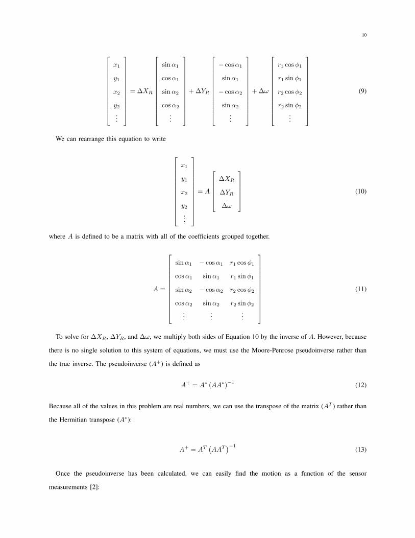
First, we write the system based on Equations 7 and 8 in matrix form:

10

x1

y1

x2

y2...

= ∆XR

sinα1

cosα1

sinα2

cosα2

...

+ ∆YR

− cosα1

sinα1

− cosα2

sinα2

...

+ ∆ω

r1 cosφ1

r1 sinφ1

r2 cosφ2

r2 sinφ2...

(9)

We can rearrange this equation to write

x1

y1

x2

y2...

= A

∆XR

∆YR

∆ω

(10)

where A is defined to be a matrix with all of the coefficients grouped together.

A =

sinα1

cosα1

sinα2

cosα2

...

− cosα1

sinα1

− cosα2

sinα2

...

r1 cosφ1

r1 sinφ1

r2 cosφ2

r2 sinφ2...

(11)

To solve for ∆XR, ∆YR, and ∆ω, we multiply both sides of Equation 10 by the inverse of A. However, because

there is no single solution to this system of equations, we must use the Moore-Penrose pseudoinverse rather than

the true inverse. The pseudoinverse (A+) is defined as

A+ = A∗ (AA∗)−1 (12)

Because all of the values in this problem are real numbers, we can use the transpose of the matrix (AT ) rather than

the Hermitian transpose (A∗):

A+ = AT(AAT

)−1(13)

Once the pseudoinverse has been calculated, we can easily find the motion as a function of the sensor

measurements [2]:

11

∆XR

∆YR

∆ω

= A+

x1

y1

x2

y2...

(14)

Once the robot’s relative motion is determined, translating this value back to absolute coordinates is trivial. This

algorithm was modeled with MATLAB, and example results are shown in Appendix C.

IV. ERROR REDUCTION

Although the individual sensors are very accurate and averaging them together provides even greater accuracy,

they are still subject to errors. Ideally, the system should detect which sensor readings are incorrect and discard

them in favor of measurements known to be more correct. There are several techniques which we can use to detect

these errors, which are described in the following sections.

After detecting the errors, we must account for them in the position estimation algorithm described in the previous

section. To do this, we extend the linear-least-squares algorithm to be a weighted linear-least-squares algorithm. That

is, rather than trying to make the solution fit all of the points equally, it favors some over others. Each measurement

is given a weight: A high weighting factor causes the derived equation to fit a data point very closely (at the expense

of a looser fit at other points), while a factor of zero forces a data point to be completely ignored.

A. Integration of multiple sensors

In [7], several assumptions are made about the characteristics of the mouse sensors which are used to detect and

correct for errors. In general, mouse sensors do not measure a distance greater than the actual distance traveled. The

optical flow algorithm may miss counts due to poor focus or insufficient frame overlap, but it will not overestimate

the motion. Thus, when there is disagreement between one or more sensors, the sensor with the higher measurement

is probably correct.

B. Use of encoder data

The proposed robot system also has a pair of rotary encoders placed on the wheels, which provide very precise

angular measurement (8192 counts per revolution). In the same way that multiple mouse sensors can be compared

against each other to determine which is more accurate, the mouse sensors can be compared against the encoder

readings to detect errors.

12

Except for rare circumstances when quickly decelerating, the robot will not move further than indicated by the

encoders. In almost all situations, wheel slip will cause the encoders to measure a distance equal to or higher than

the actual. By contrast, the mouse sensors will measure a value less than or equal to the actual. Thus if the mouse

sensors and encoders agree exactly, then the motion estimate is very good. If they disagree, there is an error -

although the system cannot directly determine whether the encoder or mouse (or both) is incorrect.

C. Use of surface quality

Each mouse sensor also provides an estimate of its accuracy - the SQUAL reading. In general, lower surface

qualities will result in lower measured distances for a given speed. At one extreme, an SQUAL reading of zero

indicates that the sensor has no features to track, and thus it will fail to report any motion. The robot can average

surface quality measurements from all of the sensors, and then lower the weights of the sensors with below-average

surface qualities. Any sensor with a surface quality in the single digits should be completely ignored.

V. ADDITIONAL USES

Besides its obvious use as a motion tracking sensor, the Avago mouse chips have other unexploited applications

on mobile robots. In [17], it is shown by reading the shutter value, the mouse sensor can be used to detect light

and dark areas on the surface. The shutter readings can be interleaved with motion readings, allowing our motion

tracking sensors to simultaneously double as line following sensors. Figure 6 shows a plot of the surface brightness

as the sensor was moved over a dark line. When the sensor is over the line, the shutter time reaches its maximum,

and the surface quality drops to about 15. By monitoring these readings, the robot can easily differentiate white

and black surfaces.

0 50 100 150 200 2500

15

120

Measurement number (Sampled at 100Hz)

Surf

ace Q

ualit

y

0 50 100 150 200 2500

2000

12000

Brightn

ess

Figure 6: Plot of the shutter value as the mouse was moved across a black line. Higher brightness values indicatedarker surfaces, i.e, longer shutter times.

13

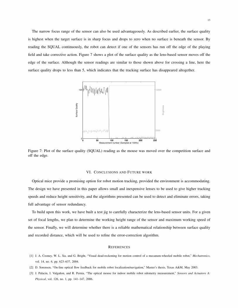
The narrow focus range of the sensor can also be used advantageously. As described earlier, the surface quality

is highest when the target surface is in sharp focus and drops to zero when no surface is beneath the sensor. By

reading the SQUAL continuously, the robot can detect if one of the sensors has run off the edge of the playing

field and take corrective action. Figure 7 shows a plot of the surface quality as the lens-based sensor moves off the

edge of the surface. Although the sensor readings are similar to those shown above for crossing a line, here the

surface quality drops to less than 5, which indicates that the tracking surface has disappeared altogether.

0 50 100 150 200 2500

120

Measurement number (Sampled at 100Hz)

Surf

ace Q

ualit

y

0 50 100 150 200 2500

2000

12000

Brightn

ess

Figure 7: Plot of the surface quality (SQUAL) reading as the mouse was moved over the competition surface andoff the edge.

VI. CONCLUSIONS AND FUTURE WORK

Optical mice provide a promising option for robot motion tracking, provided the environment is accommodating.

The design we have presented in this paper allows small and inexpensive lenses to be used to give higher tracking

speeds and reduce height sensitivity, and the algorithms presented can be used to detect and eliminate errors, taking

full advantage of sensor redundancy.

To build upon this work, we have built a test jig to carefully characterize the lens-based sensor units. For a given

set of focal lengths, we plan to determine the working height range of the sensor and maximum working speed of

the sensor. Finally, we will determine whether there is a reliable mathematical relationship between surface quality

and recorded distance, which will be used to refine the error-correction algorithm.

REFERENCES

[1] J. A. Cooney, W. L. Xu, and G. Bright, “Visual dead-reckoning for motion control of a mecanum-wheeled mobile robot,” Mechatronics,

vol. 14, no. 6, pp. 623–637, 2004.

[2] D. Sorensen, “On-line optical flow feedback for mobile robot localization/navigation,” Master’s thesis, Texas A&M, May 2003.

[3] J. Palacin, I. Valgañon, and R. Pernia, “The optical mouse for indoor mobile robot odometry measurement,” Sensors and Actuators A:

Physical, vol. 126, no. 1, pp. 141–147, 2006.

14

[4] U. Minoni and A. Signorini, “Low-cost optical motion sensors: An experimental characterization,” Sensors and Actuators A: Physical, vol.

128, no. 2, pp. 402–408, 2006.

[5] Avago ADNS-9500 Datasheet, Avago Technologies. [Online]. Available: http://www.avagotech.com/docs/AV02-1726EN

[6] Company history. Avago Technologies. [Online]. Available: http://www.avagotech.com/pages/corporate/company_history/

[7] A. Bonarini, M. Matteucci, and M. Restelli, “Automatic error detection and reduction for an odometric sensor based on two optical mice,”

in Robotics and Automation, 2005. ICRA 2005. Proceedings of the 2005 IEEE International Conference on, Apr. 2005, pp. 1675–1680.

[8] J.-S. Hu, Y.-J. Chang, and Y.-L. Hsu, “Calibration and on-line data selection of multiple optical flow sensors for mobile robot localization,”

in Intelligent Robots and Systems, 2008. IROS 2008. IEEE/RSJ International Conference on, Sep. 2008, pp. 987 –992.

[9] S. Lee, “Mobile robot localization using optical mice,” in Robotics, Automation and Mechatronics, 2004 IEEE Conference on, vol. 2, Dec.

2004, pp. 1192–1197.

[10] S. Kim and S. Lee, “Robust mobile robot velocity estimation using redundant number of optical mice,” in Information and Automation,

2008. ICIA 2008. International Conference on, Jun. 2008, pp. 107–112.

[11] D. Sekimori and F. Miyazaki, “Precise dead-reckoning for mobile robots using multiple optical mouse sensors,” in Informatics in Control,

Automation and Robotics II, J. Filipe, J.-L. Ferrier, J. A. Cetto, and M. Carvalho, Eds. Springer Netherlands, 2007, pp. 145–151.

[12] S. Singh and K. Waldron, “Design and evaluation of an integrated planar localization method for desktop robotics,” in Robotics and

Automation, 2004. Proceedings. ICRA ’04. 2004 IEEE International Conference on, vol. 2, May 2004, pp. 1109–1114.

[13] N. Tunwattana, A. Roskilly, and R. Norman, “Investigations into the effects of illumination and acceleration on optical mouse sensors as

contact-free 2d measurement devices,” Sensors and Actuators A: Physical, vol. 149, no. 1, pp. 87–92, 2009.

[14] J. Bradshaw, C. Lollini, and B. Bishop, “On the development of an enhanced optical mouse sensor for odometry and mobile robotics

education,” in System Theory, 2007. SSST ’07. Thirty-Ninth Southeastern Symposium on, Mar. 2007, pp. 6–10.

[15] S. Thakoor, J. Morookian, J. Chahl, D. Soccol, B. Hine, and S. Zornetzer, “Insect-inspired optical-flow navigation sensors,” NASA Jet

Propulsion Laboratory, Tech. Rep. NPO-40173, Oct. 2005.

[16] M. Cimino and P. Pagilla, “Location of optical mouse sensors on mobile robots for odometry,” in Robotics and Automation (ICRA), 2010

IEEE International Conference on, May 2010, pp. 5429–5434.

[17] M. Tresanchez, T. Pallejà, M. Teixidó, and J. Palacín, “The optical mouse sensor as an incremental rotary encoder,” Sensors and Actuators

A: Physical, vol. 155, no. 1, pp. 73–81, 2009.

[18] Avago ADNS-2610 Datasheet, Avago Technologies. [Online]. Available: http://www.avagotech.com/docs/AV02-1184EN

15

APPENDIX

A. Optical mouse theory of operation

An optical mouse chip consists of a tiny camera, a digital signal processing (DSP) engine, a serial interface,

and appropriate electronics to regulate power and drive the illumination LED. The camera runs at a frame rate of

over one thousand frames per second, capturing a grayscale image of a tiny patch of the tracking surface. The DSP

engine continuously compares each frame to the one before it, using optical flow algorithms to estimate the relative

motion of the sensor. Figure 8 shows two images of the letter ‘e’ in size 6 font with a small amount of movement

between the two frames. The DSP hardware within the chip compares these two images and determines that the

mouse has moved about two pixels to the right.

Figure 8: Two images captured from a modified mouse with a tiny amount of movement between them.

A cross section of a typical mouse is shown in Figure 9. The sensor, clip, LED, and lens/light pipe are all

provided by Avago Technologies; the mouse manufacturer supplies the baseplate, plastic shell, buttons, scroll wheel,

and typically the PC interface hardware.

Figure 9: Cross section of a typical optical mouse. Image taken from the Avago ADNS-2610 datasheet [18].

Laser mice work on identical principles, but use a small infrared laser for illumination rather than a visible-light

LED. The laser produces a much sharper image and brings out surface features more clearly, which is why laser

mice typically have better tracking performance on smooth surfaces than traditional optical mice. Optical mice were

used in this work because they are more commonly available and it is easier to provide visible-light illumination.

A comparison of several Avago sensors is shown in Table I.

B. Lens comparison and selection

An important part of the sensor package design is the selection and placement of the lens. The primary criterion

is that the lens provide a magnification that increases the maximum tracking speed of the sensor. A second criterion

16

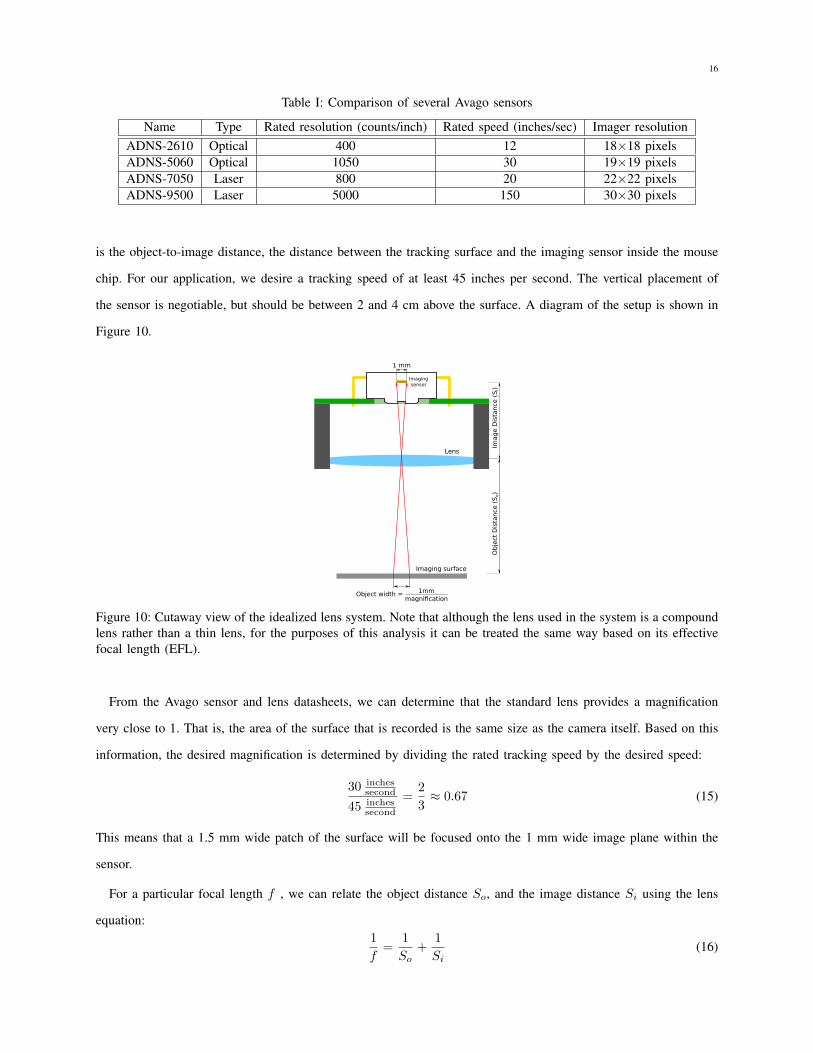
Table I: Comparison of several Avago sensors

Name Type Rated resolution (counts/inch) Rated speed (inches/sec) Imager resolutionADNS-2610 Optical 400 12 18×18 pixelsADNS-5060 Optical 1050 30 19×19 pixelsADNS-7050 Laser 800 20 22×22 pixelsADNS-9500 Laser 5000 150 30×30 pixels

is the object-to-image distance, the distance between the tracking surface and the imaging sensor inside the mouse

chip. For our application, we desire a tracking speed of at least 45 inches per second. The vertical placement of

the sensor is negotiable, but should be between 2 and 4 cm above the surface. A diagram of the setup is shown in

Figure 10.

Imaging surface

Lens

Imagingsensor

1 mm

1mmmagnification

Ob

ject

Dis

tan

ce (

So)

Imag

e D

ista

nce

(S

i)

Object width =

Figure 10: Cutaway view of the idealized lens system. Note that although the lens used in the system is a compoundlens rather than a thin lens, for the purposes of this analysis it can be treated the same way based on its effectivefocal length (EFL).

From the Avago sensor and lens datasheets, we can determine that the standard lens provides a magnification

very close to 1. That is, the area of the surface that is recorded is the same size as the camera itself. Based on this

information, the desired magnification is determined by dividing the rated tracking speed by the desired speed:

30 inchessecond

45 inchessecond

=2

3≈ 0.67 (15)

This means that a 1.5 mm wide patch of the surface will be focused onto the 1 mm wide image plane within the

sensor.

For a particular focal length f , we can relate the object distance So, and the image distance Si using the lens

equation:1

f=

1

So+

1

Si(16)

17

We also know that the magnification, m, is given by

m =Si

So(17)

Combining equations 16 and 17 we get1

f=

1

So+

1

m · So(18)

and solving for So gives us

So = f +f

m(19)

We can find Si using Equation 17 and add So and Si to find the total object-to-image distance. This set of equations

is plotted in Figure 11 for a series of commonly available focal lengths.

0 500 1000 1500 2000 2500 3000 35000

10

20

30

40

50

60

70

80

90

100

Speed (mm/second)

Obj

ect−

to−i

mag

edi

stan

ce(m

m)

f=16mm

f=12mm

f=8mm

f=6mm

f=4mm

f=2mmf=2.8mmf=3.6mm

Figure 11: Plot of the object-to-image distance as a function of focal length and tracking speed. Each line representsa particular fixed focal length. The vertical dashed line shows a magnification of 1, which gives the rated trackingspeed of 30 inches per second (762 mm

second ).

Figure 12 compares the images captured from the sensor using a constant height above the surface and varying

focal lengths. Lower focal lengths provide a wider view; high focal lengths provide a “zoomed in” view.

Based on Figure 11, a focal length of 6 mm is most appropriate for the ADNS-5060. The ADNS-2610 used in

the experiments has a tracking speed of only 12 inches per second (304.80 mmsecond ), so a larger magnification is

necessary. A focal length of 3.6 mm was selected for testing.

C. Mouse motion simulations

This section describes some example motion simulations developed in MATLAB. In each diagram, the large

rectangle represents the robot base, and each trapezoid represents a mouse sensor where the “front” of the sensor

18

(a) 3.6 mm (b) 4.0 mm (c) 6.0 mm

Figure 12: Comparison of focal lengths. The sensor PCB was placed 1.0 inches above a piece of paper with 6-pointtype, and each lens was focused appropriately.

faces the narrow end of the trapezoid. The lines indicate the motion sensed by each mouse, and the line from the

center of the robot shows the calculated motion vector. X and Y axis reference marks are drawn on the base to

indicate rotation.

The simulations in Figure 13 show only four mice for simplicity, but the code can handle any number of mice.

(a) Trivial solution, where all fourmice report the same motion.

(b) The left side moves but theright side does not, indicating bothrotation and translation.

(c) Each sensor reports a differ-ent value, indicating rotation withvery little translation.

(d) Example of sensor weighting: thelower-right sensor was given a weightof zero, so its measurement is ignored.

Figure 13: Example motion simulations calculated and drawn with MATLAB.