High-Performance Large-Scale Image Recognition Without Normalization

Andrew Brock 1 Soham De 1 Samuel L. Smith 1 Karen Simonyan 1

AbstractBatch normalization is a key component of mostimage classification models, but it has many unde-sirable properties stemming from its dependenceon the batch size and interactions between ex-amples. Although recent work has succeededin training deep ResNets without normalizationlayers, these models do not match the test ac-curacies of the best batch-normalized networks,and are often unstable for large learning ratesor strong data augmentations. In this work, wedevelop an adaptive gradient clipping techniquewhich overcomes these instabilities, and design asignificantly improved class of Normalizer-FreeResNets. Our smaller models match the test ac-curacy of an EfficientNet-B7 on ImageNet whilebeing up to 8.7× faster to train, and our largestmodels attain a new state-of-the-art top-1 accu-racy of 86.5%. In addition, Normalizer-Free mod-els attain significantly better performance thantheir batch-normalized counterparts when fine-tuning on ImageNet after large-scale pre-trainingon a dataset of 300 million labeled images, withour best models obtaining an accuracy of 89.2%.2

1. IntroductionThe vast majority of recent models in computer vision arevariants of deep residual networks (He et al., 2016b;a),trained with batch normalization (Ioffe & Szegedy, 2015).The combination of these two architectural innovations hasenabled practitioners to train significantly deeper networkswhich can achieve higher accuracies on both the trainingset and the test set. Batch normalization also smoothens theloss landscape (Santurkar et al., 2018), which enables stabletraining with larger learning rates and at larger batch sizes(Bjorck et al., 2018; De & Smith, 2020), and it can have aregularizing effect (Hoffer et al., 2017; Luo et al., 2018).

1DeepMind, London, United Kingdom. Correspondence to:Andrew Brock <ajbrock@google.com>.

2Code available at https://github.com/deepmind/deepmind-research/tree/master/nfnets

0.0 0.2 0.4 0.6 0.8 1.0 1.2 1.4Training Latency (s/step) on TPUv3, Batch Size per Device = 32

80

81

82

83

84

85

86

87

Imag

eNet

Top

-1 A

ccur

acy

(%)

F0

F1F2

F3 F4 NFNet-F5

LambdaNet-152

LambdaNet-420

EffNet-B2

EffNet-B5

EffNet-B7

BoTNet-59

BoTNet-128-T7

DeIT-224

DeIT-384

Figure 1. ImageNet Validation Accuracy vs Training Latency.All numbers are single-model, single crop. Our NFNet-F1 modelachieves comparable accuracy to an EffNet-B7 while being 8.7×faster to train. Our NFNet-F5 model has similar training latency toEffNet-B7, but achieves a state-of-the-art 86.0% top-1 accuracyon ImageNet. We further improve on this using Sharpness AwareMinimization (Foret et al., 2021) to achieve 86.5% top-1 accuracy.

However, batch normalization has three significant practicaldisadvantages. First, it is a surprisingly expensive computa-tional primitive, which incurs memory overhead (Rota Buloet al., 2018), and significantly increases the time required toevaluate the gradient in some networks (Gitman & Ginsburg,2017). Second, it introduces a discrepancy between the be-haviour of the model during training and at inference time(Summers & Dinneen, 2019; Singh & Shrivastava, 2019),introducing hidden hyper-parameters that have to be tuned.Third, and most importantly, batch normalization breaks theindependence between training examples in the minibatch.

This third property has a range of negative consequences.For instance, practitioners have found that batch normalizednetworks are often difficult to replicate precisely on differ-ent hardware, and batch normalization is often the cause ofsubtle implementation errors, especially during distributedtraining (Pham et al., 2019). Furthermore, batch normal-ization cannot be used for some tasks, since the interactionbetween training examples in a batch enables the network to‘cheat’ certain loss functions. For example, batch normaliza-tion requires specific care to prevent information leakage in

arX

iv:2

102.

0617

1v1

[cs

.CV

] 1

1 Fe

b 20

21

High-Performance Normalizer-Free ResNets

some contrastive learning algorithms (Chen et al., 2020; Heet al., 2020). This is a major concern for sequence modelingtasks as well, which has driven language models to adopt al-ternative normalizers (Ba et al., 2016; Vaswani et al., 2017).The performance of batch-normalized networks can alsodegrade if the batch statistics have a large variance duringtraining (Shen et al., 2020). Finally, the performance ofbatch normalization is sensitive to the batch size, and batchnormalized networks perform poorly when the batch size istoo small (Hoffer et al., 2017; Ioffe, 2017; Wu & He, 2018),which limits the maximum model size we can train on finitehardware. We expand on the challenges associated withbatch normalization in Appendix B.

Therefore, although batch normalization has enabled thedeep learning community to make substantial gains in re-cent years, we anticipate that in the long term it is likely toimpede progress. We believe the community should seekto identify a simple alternative which achieves competitivetest accuracies and can be used for a wide range of tasks.Although a number of alternative normalizers have been pro-posed (Ba et al., 2016; Wu & He, 2018; Huang et al., 2020),these alternatives often achieve inferior test accuracies andintroduce their own disadvantages, such as additional com-pute costs at inference. Fortunately, in recent years twopromising research themes have emerged. The first studiesthe origin of the benefits of batch normalization during train-ing (Balduzzi et al., 2017; Santurkar et al., 2018; Bjorcket al., 2018; Luo et al., 2018; Yang et al., 2019; Jacot et al.,2019; De & Smith, 2020), while the second seeks to traindeep ResNets to competitive accuracies without normaliza-tion layers (Hanin & Rolnick, 2018; Zhang et al., 2019a; De& Smith, 2020; Shao et al., 2020; Brock et al., 2021).

A key theme in many of these works is that it is possible totrain very deep ResNets without normalization by suppress-ing the scale of the hidden activations on the residual branch.The simplest way to achieve this is to introduce a learnablescalar at the end of each residual branch, initialized to zero(Goyal et al., 2017; Zhang et al., 2019a; De & Smith, 2020;Bachlechner et al., 2020). However this trick alone is notsufficient to obtain competitive test accuracies on challeng-ing benchmarks. Another line of work has shown that ReLUactivations introduce a ‘mean shift’, which causes the hid-den activations of different training examples to become in-creasingly correlated as the network depth increases (Huanget al., 2017; Jacot et al., 2019). In a recent work, Brock et al.(2021) introduced “Normalizer-Free” ResNets, which sup-press the residual branch at initialization and apply ScaledWeight Standardization (Qiao et al., 2019) to remove themean shift. With additional regularization, these unnormal-ized networks match the performance of batch-normalizedResNets (He et al., 2016a) on ImageNet (Russakovsky et al.,2015), but they are not stable at large batch sizes and do notmatch the performance of EfficientNets (Tan & Le, 2019),

the current state of the art (Gong et al., 2020). This paperbuilds on this line of work and seeks to address these centrallimitations. Our main contributions are as follows:

• We propose Adaptive Gradient Clipping (AGC), whichclips gradients based on the unit-wise ratio of gradientnorms to parameter norms, and we demonstrate thatAGC allows us to train Normalizer-Free Networks withlarger batch sizes and stronger data augmentations.

• We design a family of Normalizer-Free ResNets, calledNFNets, which set new state-of-the-art validation ac-curacies on ImageNet for a range of training latencies(See Figure 1). Our NFNet-F1 model achieves similaraccuracy to EfficientNet-B7 while being 8.7× faster totrain, and our largest model sets a new overall state ofthe art without extra data of 86.5% top-1 accuracy.

• We show that NFNets achieve substantially highervalidation accuracies than batch-normalized networkswhen fine-tuning on ImageNet after pre-training on alarge private dataset of 300 million labelled images.Our best model achieves 89.2% top-1 after fine-tuning.

The paper is structured as follows. We discuss the bene-fits of batch normalization in Section 2, and recent workseeking to train ResNets without normalization in Section 3.We introduce AGC in Section 4, and we describe how wedeveloped our new state-of-the-art architectures in Section 5.Finally, we present our experimental results in Section 6.

2. Understanding Batch NormalizationIn order to train networks without normalization to com-petitive accuracy, we must understand the benefits batchnormalization brings during training, and identify alterna-tive strategies to recover these benefits. Here we list the fourmain benefits which have been identified by prior work.

Batch normalization downscales the residual branch:The combination of skip connections (Srivastava et al.,2015; He et al., 2016b;a) and batch normalization (Ioffe &Szegedy, 2015) enables us to train significantly deeper net-works with thousands of layers (Zhang et al., 2019a). Thisbenefit arises because batch normalization, when placed onthe residual branch (as is typical), reduces the scale of hid-den activations on the residual branches at initialization (De& Smith, 2020). This biases the signal towards the skip path,which ensures that the network has well-behaved gradientsearly in training, enabling efficient optimization (Balduzziet al., 2017; Hanin & Rolnick, 2018; Yang et al., 2019).

Batch normalization eliminates mean-shift: Activationfunctions like ReLUs or GELUs (Hendrycks & Gimpel,2016), which are not anti-symmetric, have non-zero meanactivations. Consequently, the inner product between the

High-Performance Normalizer-Free ResNets

activations of independent training examples immediatelyafter the non-linearity is typically large and positive, evenif the inner product between the input features is close tozero. This issue compounds as the network depth increases,and introduces a ‘mean-shift’ in the activations of differenttraining examples on any single channel proportional to thenetwork depth (De & Smith, 2020), which can cause deepnetworks to predict the same label for all training examplesat initialization (Jacot et al., 2019). Batch normalization en-sures the mean activation on each channel is zero across thecurrent batch, eliminating mean shift (Brock et al., 2021).

Batch normalization has a regularizing effect: It iswidely believed that batch normalization also acts as a regu-larizer enhancing test set accuracy, due to the noise in thebatch statistics which are computed on a subset of the train-ing data (Luo et al., 2018). Consistent with this perspective,the test accuracy of batch-normalized networks can often beimproved by tuning the batch size, or by using ghost batchnormalization in distributed training (Hoffer et al., 2017).

Batch normalization allows efficient large-batch train-ing: Batch normalization smoothens the loss landscape(Santurkar et al., 2018), and this increases the largest stablelearning rate (Bjorck et al., 2018). While this property doesnot have practical benefits when the batch size is small (De& Smith, 2020), the ability to train at larger learning rates isessential if one wishes to train efficiently with large batchsizes. Although large-batch training does not achieve highertest accuracies within a fixed epoch budget (Smith et al.,2020), it does achieve a given test accuracy in fewer param-eter updates, significantly improving training speed whenparallelized across multiple devices (Goyal et al., 2017).

3. Towards Removing Batch NormalizationMany authors have attempted to train deep ResNets to com-petitive accuracies without normalization, by recoveringone or more of the benefits of batch normalization describedabove. Most of these works suppress the scale of the activa-tions on the residual branch at initialization, by introducingeither small constants or learnable scalars (Hanin & Rol-nick, 2018; Zhang et al., 2019a; De & Smith, 2020; Shaoet al., 2020). Additionally, Zhang et al. (2019a) and De &Smith (2020) observed that the performance of unnormal-ized ResNets can be improved with additional regulariza-tion. However only recovering these two benefits of batchnormalization is not sufficient to achieve competitive testaccuracies on challenging benchmarks (De & Smith, 2020).

In this work, we adopt and build on “Normalizer-FreeResNets” (NF-ResNets) (Brock et al., 2021), a class of pre-activation ResNets (He et al., 2016a) which can be trained tocompetitive training and test accuracies without normaliza-tion layers. NF-ResNets employ a residual block of the form

hi+1 = hi +αfi(hi/βi), where hi denotes the inputs to theith residual block, and fi denotes the function computedby the ith residual branch. The function fi is parameter-ized to be variance preserving at initialization, such thatVar(fi(z)) = Var(z) for all i. The scalar α specifies therate at which the variance of the activations increases aftereach residual block (at initialization), and is typically set to asmall value like α = 0.2. The scalar βi is determined by pre-dicting the standard deviation of the inputs to the ith residualblock, βi =

√Var(hi), where Var(hi+1) = Var(hi) + α2,

except for transition blocks (where spatial downsamplingoccurs), for which the skip path operates on the downscaledinput (hi/βi), and the expected variance is reset after thetransition block to hi+1 = 1 + α2. The outputs of squeeze-excite layers (Hu et al., 2018) are multiplied by a factor of 2.Empirically, Brock et al. (2021) found it was also beneficialto include a learnable scalar initialized to zero at the end ofeach residual branch (‘SkipInit’ (De & Smith, 2020)).

In addition, Brock et al. (2021) prevent the emergence of amean-shift in the hidden activations by introducing ScaledWeight Standardization (a minor modification of WeightStandardization (Huang et al., 2017; Qiao et al., 2019)).This technique reparameterizes the convolutional layers as:

Wij =Wij − µi√

Nσi, (1)

where µi = (1/N)∑

j Wij , σ2i = (1/N)

∑j(Wij − µi)

2,and N denotes the fan-in. The activation functions arealso scaled by a non-linearity specific scalar gain γ, whichensures that the combination of the γ-scaled activation func-tion and a Scaled Weight Standardized layer is variancepreserving. For ReLUs, γ =

√2/(1− (1/π)) (Arpit et al.,

2016). We refer the reader to Brock et al. (2021) for adescription of how to compute γ for other non-linearities.

With additional regularization (Dropout (Srivastava et al.,2014) and Stochastic Depth (Huang et al., 2016)),Normalizer-Free ResNets match the test accuracies achievedby batch normalized pre-activation ResNets on ImageNetat batch size 1024. They also significantly outperform theirbatch normalized counterparts when the batch size is verysmall, but they perform worse than batch normalized net-works for large batch sizes (4096 or higher). Crucially, theydo not match the performance of state-of-the-art networkslike EfficientNets (Tan & Le, 2019; Gong et al., 2020).

4. Adaptive Gradient Clipping for EfficientLarge-Batch Training

To scale NF-ResNets to larger batch sizes, we explore arange of gradient clipping strategies (Pascanu et al., 2013).Gradient clipping is often used in language modeling to sta-bilize training (Merity et al., 2018), and recent work showsthat it allows training with larger learning rates compared

High-Performance Normalizer-Free ResNets

to gradient descent, accelerating convergence (Zhang et al.,2020). This is particularly important for poorly conditionedloss landscapes or when training with large batch sizes, sincein these settings the optimal learning rate is constrained bythe maximum stable learning rate (Smith et al., 2020). Wetherefore hypothesize that gradient clipping should helpscale NF-ResNets efficiently to the large-batch setting.

Gradient clipping is typically performed by constraining thenorm of the gradient (Pascanu et al., 2013). Specifically, forgradient vector G = ∂L/∂θ, where L denotes the loss andθ denotes a vector with all model parameters, the standardclipping algorithm clips the gradient before updating θ as:

G→

{λ G‖G‖ if ‖G‖ > λ,

G otherwise.(2)

The clipping threshold λ is a hyper-parameter which mustbe tuned. Empirically, we found that while this clipping al-gorithm enabled us to train at higher batch sizes than before,training stability was extremely sensitive to the choice ofthe clipping threshold, requiring fine-grained tuning whenvarying the model depth, the batch size, or the learning rate.

To overcome this issue, we introduce “Adaptive Gra-dient Clipping” (AGC), which we now describe. LetW ` ∈ RN×M denote the weight matrix of the `th layer,G` ∈ RN×M denote the gradient with respect to W `,and ‖ · ‖F denote the Frobenius norm, i.e., ‖W `‖F =√∑N

i

∑Mj (W `

i,j)2. The AGC algorithm is motivated by

the observation that the ratio of the norm of the gradientsG`

to the norm of the weights W ` of layer `, ‖G`‖F

‖W `‖F , providesa simple measure of how much a single gradient descentstep will change the original weights W `. For instance, ifwe train using gradient descent without momentum, then‖∆W `‖‖W `‖ = h ‖G

`‖F‖W `‖F , where the parameter update for the `th

layer is given by ∆W ` = −hG`, and h is the learning rate.

Intuitively, we expect training to become unstable if(‖∆W `‖/‖W `‖) is large, which motivates a clipping strat-egy based on the ratio ‖G

`‖F‖W `‖F . However in practice, we clip

gradients based on the unit-wise ratios of gradient norms toparameter norms, which we found to perform better empiri-cally than taking layer-wise norm ratios. Specifically, in ourAGC algorithm, each unit i of the gradient of the `-th layerG`

i (defined as the ith row of matrix G`) is clipped as:

G`i →

{λ‖W `

i ‖?F

‖G`i‖F

G`i if ‖G

`i‖F

‖W `i ‖?F

> λ,

G`i otherwise.

(3)

The clipping threshold λ is a scalar hyperparameter, and wedefine ‖Wi‖?F = max(‖Wi‖F , ε), with default ε = 10−3,which prevents zero-initialized parameters from always hav-ing their gradients clipped to zero. For parameters in con-volutional filters, we evaluate the unit-wise norms over the

256 512 1024 2048 4096Batch Size B

70

72

74

76

78

80

Top-

1 Ac

cura

cy

BatchNormNF-ResNetNF-ResNet+AGCResNet50ResNet200

(a)

0.01 0.02 0.04 0.08 0.16Clipping Threshold

74

75

76

77

Top-

1 Ac

cura

cy

ResNet50

B = 256B = 512B = 1024B = 2048B = 4096

(b)

Figure 2. (a) AGC efficiently scales NF-ResNets to larger batchsizes. (b) The performance across different clipping thresholds λ.

fan-in extent (including the channel and spatial dimensions).Using AGC, we can train NF-ResNets stably with largerbatch sizes (up to 4096), as well as with very strong dataaugmentations like RandAugment (Cubuk et al., 2020) forwhich NF-ResNets without AGC fail to train (Brock et al.,2021). Note that the optimal clipping parameter λ may de-pend on the choice of optimizer, learning rate and batch size.Empirically, we find λ should be smaller for larger batches.

AGC is closely related to a recent line of work studying “nor-malized optimizers” (You et al., 2017; Bernstein et al., 2020;You et al., 2019), which ignore the scale of the gradient bychoosing an adaptive learning rate inversely proportional tothe gradient norm. In particular, You et al. (2017) proposeLARS, a momentum variant which sets the norm of theparameter update to be a fixed ratio of the parameter norm,completely ignoring the gradient magnitude. AGC can beinterpreted as a relaxation of normalized optimizers, whichimposes a maximum update size based on the parameternorm but does not simultaneously impose a lower-boundon the update size or ignore the gradient magnitude. Al-though we are also able to stably train at high batch sizeswith LARS, we found that doing so degrades performance.

4.1. Ablations for Adaptive Gradient Clipping (AGC)

We now present a range of ablations designed to test the effi-cacy of AGC. We performed experiments on pre-activationNF-ResNet-50 and NF-ResNet-200 on ImageNet, trainedusing SGD with Nesterov’s Momentum for 90 epochs at arange of batch sizes between 256 and 4096. As in Goyalet al. (2017) we use a base learning rate of 0.1 for batchsize 256, which is scaled linearly with the batch size. Weconsider a range of λ values [0.01, 0.02, 0.04, 0.08, 0.16].

In Figure 2(a), we compare batch-normalized ResNets toNF-ResNets with and without AGC. We show test accuracyat the best clipping threshold λ for each batch size. We findthat AGC helps scale NF-ResNets to large batch sizes whilemaintaining performance comparable or better than batch-normalized networks on both ResNet50 and ResNet200. Asanticipated, the benefits of using AGC are smaller when thebatch size is small. In Figure 2(b), we show performance

High-Performance Normalizer-Free ResNets

1/𝛽 1x1 3x3 3x3 1x1 𝛼

+

Stage Widths:ResNet: [256, 512, 1024, 2048]NFNet: [256, 512, 1536, 1536]

Stage Depths:ResNet: [3, 4, 6, 3], [3, 4, 23, 3]...NFNet: [1, 2, 6, 3] * N

Figure 3. Summary of NFNet bottleneck block design and archi-tectural differences. See Figure 5 in Appendix C for more details.

for different clipping thresholds λ across a range of batchsizes on ResNet50. We see that smaller (stronger) clippingthresholds are necessary for stability at higher batch sizes.We provide additional ablation details in Appendix D.

Next, we study whether or not AGC is beneficial for alllayers. Using batch size 4096 and a clipping thresholdλ = 0.01, we remove AGC from different combinations ofthe first convolution, the final linear layer, and every blockin any given set of the residual stages. For example, oneexperiment may remove clipping in the linear layer and allthe blocks in the second and fourth stages. Two key trendsemerge: first, it is always better to not clip the final linearlayer. Second, it is often possible to train stably withoutclipping the initial convolution, but the weights of all fourstages must be clipped to achieve stability when training atbatch size 4096 with the default learning rate of 1.6. Forthe rest of this paper (and for our ablations in Figure 2), weapply AGC to every layer except for the final linear layer.

5. Normalizer-Free Architectures withImproved Accuracy and Training Speed

In the previous section we introduced AGC, a gradient clip-ping method which allows us to train efficiently with largebatch sizes and strong data augmentations. Equipped withthis technique, we now seek to design Normalizer-Free ar-chitectures with state-of-the-art accuracy and training speed.

The current state of the art on image classification is gener-ally held by the EfficientNet family of models (Tan & Le,2019), which are based on a variant of inverted bottleneckblocks (Sandler et al., 2018) with a backbone and model scal-ing strategy derived from neural architecture search. Thesemodels are optimized to maximize test accuracy while mini-mizing parameter and FLOP counts, but their low theoreticalcompute complexity does not translate into improved train-ing speed on modern accelerators. Despite having 10x fewerFLOPS than a ResNet-50, an EffNet-B0 has similar traininglatency and final performance when trained on GPU or TPU.

The choice of which metric to optimize– theoretical FLOPS,inference latency on a target device, or training latency on anaccelerator–is a matter of preference, and the nature of eachmetric will yield different design requirements. In this workwe choose to focus on manually designing models which

Table 1. NFNet family depths, drop rates, and input resolutions.

Variant Depth Dropout Train Test

F0 [1, 2, 6, 3] 0.2 192px 256pxF1 [2, 4, 12, 6] 0.3 224px 320pxF2 [3, 6, 18, 9] 0.4 256px 352pxF3 [4, 8, 24, 12] 0.4 320px 416pxF4 [5, 10, 30, 15] 0.5 384px 512pxF5 [6, 12, 36, 18] 0.5 416px 544pxF6 [7, 14, 42, 21] 0.5 448px 576px

are optimized for training latency on existing accelerators,as in Radosavovic et al. (2020). It is possible that futureaccelerators may be able to take full advantage of the poten-tial training speed that largely goes unrealized with modelslike EfficientNets, so we believe this direction should notbe ignored (Hooker, 2020), however we anticipate that de-veloping models with improved training speed on currenthardware will be beneficial for accelerating research. Wenote that accelerators like GPU and TPU tend to favor densecomputation, and while there are differences between thesetwo platforms, they have enough in common that modelsdesigned for one device are likely to train fast on the other.

We therefore explore the space of model design by manu-ally searching for design trends which yield improvementsto the pareto front of holdout top-1 on ImageNet againstactual training latency on device. This section describes thechanges which we found to work well to this end (with moredetails in Appendix C), while the ideas which we found towork poorly are described in Appendix E. A summary ofthese modifications is presented in Figure 3, and the effectthey have on holdout accuracy is presented in Table 2.

We begin with an SE-ResNeXt-D model (Xie et al., 2017;Hu et al., 2018; He et al., 2019) with GELU activations(Hendrycks & Gimpel, 2016), which we found to be a sur-prisingly strong baseline for Normalizer-Free Networks. Wemake the following changes. First, we set the group width(the number of channels each output unit is connected to) inthe 3× 3 convs to 128, regardless of block width. Smallergroup widths reduce theoretical FLOPS, but the reduction incompute density means that on many modern acceleratorsno actual speedup is realized. On TPUv3 for example, anSE-ResNeXt-50 with a group width of 8 trains at the samespeed as an SE-ResNeXt-50 with a group width of 128 un-less the per-device batch size is 128 or larger (Google, 2021),which is often not realizable due to memory constraints.

Next, we make two changes to the model backbone. First,we note that the default depth scaling pattern for ResNets(e.g., the method by which one increases depth to constructa ResNet101 or ResNet200 from a ResNet50) involves non-uniformly increasing the number of layers in the second

High-Performance Normalizer-Free ResNets

Table 2. The effect of architectural modifications and data augmen-tation on ImageNet Top-1 accuracy (averaged over 3 seeds).

F0 F1 F2 F3

Baseline 80.4 81.7 82.0 82.3+ Modified Width 80.9 81.8 82.0 82.3+ Second Conv 81.3 82.2 82.4 82.7+ MixUp 82.2 82.9 83.1 83.5+ RandAugment 83.2 84.6 84.8 85.0+ CutMix 83.6 84.7 85.1 85.7Default Width + Augs 83.1 84.5 85.0 85.5

and third stages, while maintaining 3 blocks in the first andfourth stages, where ‘stage’ refers to a sequence of residualblocks whose activations are the same width and have thesame resolution. We find that this strategy is suboptimal.Layers in early stages operate at higher resolution, requiremore memory and compute, and tend to learn localized, task-general features (Krizhevsky et al., 2012), while layers inlater stages operate at lower resolutions, contain most of themodel’s parameters, and learn more task-specific features(Raghu et al., 2017a). However, being overly parsimoniouswith early stages (such as through aggressive downsam-pling) can hurt performance, since the model needs enoughcapacity to extract good local features (Raghu et al., 2017b).It is also desirable to have a simple scaling rule for construct-ing deeper variants (Tan & Le, 2019). With these principlesin mind, we explored several choices of backbone for oursmallest model variant, named F0, before settling on thesimple pattern [1, 2, 6, 3] (indicating how many bottleneckblocks to allocate to each stage). We construct deeper vari-ants by multiplying the depth of each stage by a scalarN , sothat, for example, variant F1 has a depth pattern [2, 4, 12, 6],and variant F4 has a depth pattern [5, 10, 30, 15].

In addition, we reconsider the default width pattern inResNets, where the first stage has 256 channels which aredoubled at each subsequent stage, resulting in a pattern[256, 512, 1024, 2048]. Employing our depth patterns de-scribed above, we considered a range of alternative pat-terns (taking inspiration from Radosavovic et al. (2020))but found that only one choice was better than this default:[256, 512, 1536, 1536]. This width pattern is designed toincrease capacity in the third stage while slightly reducingcapacity in the fourth stage, roughly preserving trainingspeed. Consistent with our chosen depth pattern and thedefault design of ResNets, we find that the third stage tendsto be the best place to add capacity, which we hypothesize isdue to this stage being deep enough to have a large receptivefield and access to deeper levels of the feature hierarchy,while having a slightly higher resolution than the final stage.

We also consider the structure of the bottleneck residualblock itself. We considered a variety of pre-existing and

novel modifications (see Appendix E) but found that the bestimprovement came from adding an additional 3×3 groupedconv after the first (with accompanying nonlinearity). Thisadditional convolution minimally impacts FLOPS and hasalmost no impact on training time on our target accelerators.

Finally, we establish a scaling strategy to produce modelvariants at different compute budgets. The EfficientNet scal-ing strategy (Tan & Le, 2019) is to jointly scale model width,depth, and input resolution, which works extremely wellfor base models with very slim MobileNet-like backbones.However we find that width scaling is ineffective for ResNetbackbones, consistent with Bello (2021), who attain strongperformance when only scaling depth and input resolution.We therefore also adopt the latter strategy, using the fixedwidth pattern mentioned above, scaling depth as describedabove, and scaling training resolution such that each vari-ant is approximately half as fast to train as its predecessor.Following Touvron et al. (2019), we evaluate images at infer-ence at a slightly higher resolution than we train at, chosenfor each variant as approximately 33% larger than the trainresolution. We do not fine-tune at this higher resolution.

We also find that it is helpful to increase the regularizationstrength as the model capacity rises. However modifying theweight decay or stochastic depth rate was not effective, andinstead we scale the drop rate of Dropout (Srivastava et al.,2014), following Tan & Le (2019). This step is particularlyimportant as our models lack the implicit regularizationof batch normalization, and without explicit regularizationtend to dramatically overfit. Our resulting models are highlyperformant and, despite being optimized for training latency,remain competitive with larger EfficientNet variants in termsof FLOPs vs accuracy (although not in terms of parametersvs accuracy), as shown in Figure 4 in Appendix A.

5.1. Summary

Our training recipe can be summarized as follows: First,apply the Normalizer-Free setup of Brock et al. (2021) toan SE-ResNeXt-D, with modified width and depth patterns,and a second spatial convolution. Second, apply AGC toevery parameter except for the linear weight of the classifierlayer. For batch size 1024 to 4096, set λ = 0.01, and makeuse of strong regularization and data augmentation. SeeTable 1 for additional information on each model variant.

6. Experiments6.1. Evaluating NFNets on ImageNet

We now turn our attention to evaluating our NFNet modelson ImageNet, beginning with an ablation of our architecturalmodifications when training for 360 epochs at batch size4096. We use Nesterov’s Momentum with a momentumcoefficient of 0.9, AGC as described in Section 4 with a

High-Performance Normalizer-Free ResNets

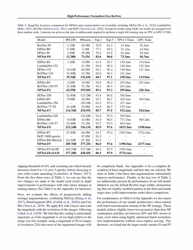
Table 3. ImageNet Accuracy comparison for NFNets and a representative set of models, including SENet (Hu et al., 2018), LambdaNet,(Bello, 2021), BoTNet (Srinivas et al., 2021), and DeIT (Touvron et al., 2020). Except for results using SAM, our results are averaged overthree random seeds. Latencies are given as the time in milliseconds required to perform a single full training step on TPU or GPU (V100).

Model #FLOPs #Params Top-1 Top-5 TPUv3 Train GPU Train

ResNet-50 4.10B 26.0M 78.6 94.3 41.6ms 35.3msEffNet-B0 0.39B 5.3M 77.1 93.3 51.1ms 44.8msSENet-50 4.09B 28.0M 79.4 94.6 64.3ms 59.4msNFNet-F0 12.38B 71.5M 83.6 96.8 73.3ms 56.7ms

EffNet-B3 1.80B 12.0M 81.6 95.7 129.5ms 116.6msLambdaNet-152 − 51.5M 83.0 96.3 138.3ms 135.2msSENet-152 19.04B 66.6M 83.1 96.4 149.9ms 151.2msBoTNet-110 10.90B 54.7M 82.8 96.3 181.3ms −NFNet-F1 35.54B 132.6M 84.7 97.1 158.5ms 133.9ms

EffNet-B4 4.20B 19.0M 82.9 96.4 245.9ms 221.6msBoTNet-128-T5 19.30B 75.1M 83.5 96.5 355.2ms −NFNet-F2 62.59B 193.8M 85.1 97.3 295.8ms 226.3ms

SENet-350 52.90B 115.2M 83.8 96.6 593.6ms −EffNet-B5 9.90B 30.0M 83.7 96.7 450.5ms 458.9msLambdaNet-350 − 105.8M 84.5 97.0 471.4ms −BoTNet-77-T6 23.30B 53.9M 84.0 96.7 578.1ms −NFNet-F3 114.76B 254.9M 85.7 97.5 532.2ms 524.5ms

LambdaNet-420 − 124.8M 84.8 97.0 593.9ms −EffNet-B6 19.00B 43.0M 84.0 96.8 775.7ms 868.2msBoTNet-128-T7 45.80B 75.1M 84.7 97.0 804.5ms −NFNet-F4 215.24B 316.1M 85.9 97.6 1033.3ms 1190.6ms

EffNet-B7 37.00B 66.0M 84.7 97.0 1397.0ms 1753.3msDeIT 1000 epochs − 87.0M 85.2 − − −EffNet-B8+MaxUp 62.50B 87.4M 85.8 − − −NFNet-F5 289.76B 377.2M 86.0 97.6 1398.5ms 2177.1ms

NFNet-F5+SAM 289.76B 377.2M 86.3 97.9 1958.0ms −NFNet-F6+SAM 377.28B 438.4M 86.5 97.9 2774.1ms −

clipping threshold of 0.01, and a learning rate which linearlyincreases from 0 to 1.6 over 5 epochs, before decaying tozero with cosine annealing (Loshchilov & Hutter, 2017).From the first three rows of Table 2, we can see that thetwo changes we make to the model each result in slightimprovements to performance with only minor changes intraining latency (See Table 6 in the Appendix for latencies).

Next, we evaluate the effects of progressively addingstronger augmentations, combining MixUp (Zhang et al.,2017), RandAugment (RA, (Cubuk et al., 2020)) and Cut-Mix (Yun et al., 2019). We apply RA with 4 layers and scalethe magnitude with the resolution of the images, followingCubuk et al. (2020). We find that this scaling is particularlyimportant, as if the magnitude is set too high relative to theimage size (for example, using a magnitude of 20 on imagesof resolution 224) then most of the augmented images will

be completely blank. See Appendix A for a complete de-scription of these magnitudes and how they are selected. Weshow in Table 2 that these data augmentations substantiallyimprove performance. Finally, in the last row of Table 2,we additionally present the performance of our full modelablated to use the default ResNet stage widths, demonstrat-ing that our slightly modified pattern in the third and fourthstages does yield improvements under direct comparison.

For completeness, in Table 6 of the Appendix we also reportthe performance of our model architectures when trainedwith batch normalization instead of the NF strategy. Thesemodels achieve slightly lower test accuracies than their NFcounterparts and they are between 20% and 40% slower totrain, even when using highly optimized batch normaliza-tion implementations without cross-replica syncing. Fur-thermore, we found that the larger model variants F4 and F5

High-Performance Normalizer-Free ResNets

were not stable when training with batch normalization, withor without AGC. We attribute this to the necessity of usingbfloat16 training to fit these larger models in memory, whichmay introduce numerical imprecision that interacts poorlywith the computation of batch normalization statistics.

We provide a detailed summary of the size, training latency(on TPUv3 and V100 with tensorcores), and ImageNet vali-dation accuracy of six model variants, NFNet-F0 throughF5, along with comparisons to other models with similartraining latencies, in Table 3. Our NFNet-F5 model attains atop-1 validation accuracy of 86.0%, improving over the pre-vious state of the art, EfficientNet-B8 with MaxUp (Gonget al., 2020) by a small margin, and our NFNet-F1 modelmatches the 84.7% of EfficientNet-B7 with RA (Cubuket al., 2020), while being 8.7 times faster to train. SeeAppendix A for details of how we measure training latency.

Our models also benefit from the recently proposedSharpness-Aware Minimization (SAM, (Foret et al., 2021)).SAM is not part of our standard training pipeline, as bydefault it doubles the training time and typically can onlybe used for distributed training. However we make a smallmodification to the SAM procedure to reduce this cost to 20-40% increased training time (explained in Appendix A) andemploy it to train our two largest model variants, resultingin an NFNet-F5 that attains 86.3% top-1, and an NFNet-F6that attains 86.5% top-1, substantially improving over theexisting state of the art on ImageNet without extra data.

Finally, we also evaluated the performance of our data aug-mentation strategy on EfficientNets. We find that while RAstrongly improves EfficientNets’ performance over base-line augmentation, increasing the number of layers beyond2 or adding MixUp and CutMix does not further improvetheir performance, suggesting that our performance improve-ments are difficult to obtain by simply using stronger dataaugmentations. We also find that using SGD with cosineannealing instead of RMSProp (Tieleman & Hinton, 2012)with step decay severely degrades EfficientNet performance,indicating that our performance improvements are also notsimply due to the selection of a different optimizer.

6.2. Evaluating NFNets under Transfer

Unnormalized networks do not share the implicit regular-ization effect of batch normalization, and on datasets likeImageNet (Russakovsky et al., 2015) they tend to overfit un-less explicitly regularized (Zhang et al., 2019a; De & Smith,2020; Brock et al., 2021). However when pre-training onextremely large scale datasets, such regularization may notonly be unnecessary, but also harmful to performance, re-ducing the model’s ability to devote its full capacity to thetraining set. We hypothesize that this may make Normalizer-Free networks naturally better suited to transfer learningafter large-scale pre-training, and investigate this via pre-

Table 4. ImageNet Transfer Top-1 accuracy after pre-training.

224px 320px 384px

BN-ResNet-50 78.1 79.6 79.9NF-ResNet-50 79.5 80.9 81.1

BN-ResNet-101 80.8 82.2 82.5NF-ResNet-101 81.4 82.7 83.2

BN-ResNet-152 81.8 83.1 83.4NF-ResNet-152 82.7 83.6 84.0

BN-ResNet-200 81.8 83.1 83.5NF-ResNet-200 82.9 84.1 84.3

training on a large dataset of 300 million labeled images.

We pre-train a range of batch normalized and NF-ResNetsfor 10 epochs on this large dataset, then fine-tune all layerson ImageNet simultaneously, using a batch size of 2048 anda small learning rate of 0.1 with cosine annealing for 15,000steps, for input image resolutions in the range [224, 320,384]. As shown in Table 4, Normalizer-Free networks out-perform their Batch-Normalized counterparts in every singlecase, typically by a margin of around 1% absolute top-1.This suggests that in the transfer learning regime, removingbatch normalization can directly benefit final performance.

We perform this same experiment using our NFNet models,pre-training an NFNet-F4 and a slightly wider variant whichwe denote NFNet-F4+ (see Appendix C). As shown in Ta-ble 5 of the appendix, with 20 epochs of pre-training ourNFNet-F4+ attains an ImageNet top-1 accuracy of 89.2%.This is the second highest validation accuracy achieved todate with extra training data, second only to a strong recentsemi-supervised learning baseline (Pham et al., 2020), andthe highest accuracy achieved using transfer learning.

ConclusionWe show for the first time that image recognition models,trained without normalization layers, can not only matchthe classification accuracies of the best batch normalizedmodels on large-scale datasets but also substantially exceedthem, while still being faster to train. To achieve this, we in-troduce Adaptive Gradient Clipping, a simple clipping algo-rithm which stabilizes large-batch training and enables us tooptimize unnormalized networks with strong data augmen-tations. Leveraging this technique and simple architecturedesign principles, we develop a family of models which at-tain state-of-the-art performance on ImageNet without extradata, while being substantially faster to train than competingapproaches. We also show that Normalizer-Free models arebetter suited to fine-tuning after pre-training on very largescale datasets than their batch-normalized counterparts.

High-Performance Normalizer-Free ResNets

AcknowledgementsWe would like to thank Aaron van den Oord, Sander Diele-man, Erich Elsen, Guillaume Desjardins, Michael Figurnov,Nikolay Savinov, Omar Rivasplata, Relja Arandjelovic, andRishub Jain for helpful discussions and guidance. Addition-ally, we would like to thank Blake Hechtman, Tim Shen,Peter Hawkins, and James Bradbury for assistance withdeveloping highly performant JAX code.

ReferencesArpit, D., Zhou, Y., Kota, B., and Govindaraju, V. Normal-

ization propagation: A parametric technique for removinginternal covariate shift in deep networks. In InternationalConference on Machine Learning, pp. 1168–1176, 2016.

Ba, J. L., Kiros, J. R., and Hinton, G. E. Layer normalization.arXiv preprint arXiv:1607.06450, 2016.

Babuschkin, I., Baumli, K., Bell, A., Bhupatiraju, S., Bruce,J., Buchlovsky, P., Budden, D., Cai, T., Clark, A., Dani-helka, I., Fantacci, C., Godwin, J., Jones, C., Hennigan,T., Hessel, M., Kapturowski, S., Keck, T., Kemaev, I.,King, M., Martens, L., Mikulik, V., Norman, T., Quan,J., Papamakarios, G., Ring, R., Ruiz, F., Sanchez, A.,Schneider, R., Sezener, E., Spencer, S., Srinivasan, S.,Stokowiec, W., and Viola, F. The DeepMind JAX Ecosys-tem, 2020. URL http://github.com/deepmind.

Bachlechner, T., Majumder, B. P., Mao, H. H., Cottrell,G. W., and McAuley, J. Rezero is all you need: Fast con-vergence at large depth. arXiv preprint arXiv:2003.04887,2020.

Balduzzi, D., Frean, M., Leary, L., Lewis, J., Ma, K. W.-D.,and McWilliams, B. The shattered gradients problem:If resnets are the answer, then what is the question? InInternational Conference on Machine Learning, pp. 342–350, 2017.

Bello, I. Lambdanetworks: Modeling long-range interac-tions without attention. In International Conference onLearning Representations ICLR, 2021. URL https://openreview.net/forum?id=xTJEN-ggl1b.

Bernstein, J., Vahdat, A., Yue, Y., and Liu, M.-Y. On thedistance between two neural networks and the stability oflearning. arXiv preprint arXiv:2002.03432, 2020.

Bjorck, N., Gomes, C. P., Selman, B., and Weinberger,K. Q. Understanding batch normalization. In Advances inNeural Information Processing Systems, pp. 7694–7705,2018.

Bradbury, J., Frostig, R., Hawkins, P., Johnson, M. J., Leary,C., Maclaurin, D., and Wanderman-Milne, S. JAX: com-

posable transformations of Python+NumPy programs,2018. URL http://github.com/google/jax.

Brock, A., De, S., and Smith, S. L. Characterizing signalpropagation to close the performance gap in unnormal-ized resnets. In 9th International Conference on LearningRepresentations, ICLR, 2021.

Chen, T., Kornblith, S., Norouzi, M., and Hinton, G. Asimple framework for contrastive learning of visual rep-resentations. In International conference on machinelearning, pp. 1597–1607. PMLR, 2020.

Cubuk, E. D., Zoph, B., Shlens, J., and Le, Q. V. Ran-daugment: Practical automated data augmentation with areduced search space. In Proceedings of the IEEE/CVFConference on Computer Vision and Pattern RecognitionWorkshops, pp. 702–703, 2020.

De, S. and Smith, S. Batch normalization biases residualblocks towards the identity function in deep networks.Advances in Neural Information Processing Systems, 33,2020.

Dosovitskiy, A., Beyer, L., Kolesnikov, A., Weissenborn,D., Zhai, X., Unterthiner, T., Dehghani, M., Minderer,M., Heigold, G., Gelly, S., Uszkoreit, J., and Houlsby, N.An image is worth 16x16 words: Transformers for imagerecognition at scale. In 9th International Conference onLearning Representations, ICLR, 2021. URL https://openreview.net/forum?id=YicbFdNTTy.

Foret, P., Kleiner, A., Mobahi, H., and Neyshabur, B.Sharpness-aware minimization for efficiently improv-ing generalization. In 9th International Conference onLearning Representations, ICLR, 2021. URL https://openreview.net/forum?id=6Tm1mposlrM.

Gitman, I. and Ginsburg, B. Comparison of batch nor-malization and weight normalization algorithms forthe large-scale image classification. arXiv preprintarXiv:1709.08145, 2017.

Gong, C., Ren, T., Ye, M., and Liu, Q. Maxup: A simpleway to improve generalization of neural network training.arXiv preprint arXiv:2002.09024, 2020.

Google. Cloud TPU Performance Guide.https://cloud.google.com/tpu/docs/performance-guide, 2021.

Goyal, P., Dollar, P., Girshick, R., Noordhuis, P.,Wesolowski, L., Kyrola, A., Tulloch, A., Jia, Y., andHe, K. Accurate, large minibatch sgd: Training imagenetin 1 hour. arXiv preprint arXiv:1706.02677, 2017.

Gueguen, L., Sergeev, A., Kadlec, B., Liu, R., and Yosinski,J. Faster neural networks straight from jpeg. Advances in

High-Performance Normalizer-Free ResNets

Neural Information Processing Systems, 31:3933–3944,2018.

Hanin, B. and Rolnick, D. How to start training: The effectof initialization and architecture. In Advances in NeuralInformation Processing Systems, pp. 571–581, 2018.

Harris, C. R., Millman, K. J., van der Walt, S. J., Gommers,R., Virtanen, P., Cournapeau, D., Wieser, E., Taylor, J.,Berg, S., Smith, N. J., Kern, R., Picus, M., Hoyer, S., vanKerkwijk, M. H., Brett, M., Haldane, A., del Rıo, J. F.,Wiebe, M., Peterson, P., Gerard-Marchant, P., Sheppard,K., Reddy, T., Weckesser, W., Abbasi, H., Gohlke, C., andOliphant, T. E. Array programming with numpy. Nature,585(7825):357–362, Sep 2020. ISSN 1476-4687.

He, K., Zhang, X., Ren, S., and Sun, J. Identity mappingsin deep residual networks. In European conference oncomputer vision, pp. 630–645. Springer, 2016a.

He, K., Zhang, X., Ren, S., and Sun, J. Deep residuallearning for image recognition. In CVPR, 2016b.

He, K., Fan, H., Wu, Y., Xie, S., and Girshick, R. Mo-mentum contrast for unsupervised visual representationlearning. In Proceedings of the IEEE/CVF Conferenceon Computer Vision and Pattern Recognition, pp. 9729–9738, 2020.

He, T., Zhang, Z., Zhang, H., Zhang, Z., Xie, J., and Li, M.Bag of tricks for image classification with convolutionalneural networks. In Proceedings of the IEEE Conferenceon Computer Vision and Pattern Recognition, pp. 558–567, 2019.

Hendrycks, D. and Gimpel, K. Gaussian error linear units(GELUs). arXiv preprint arXiv:1606.08415, 2016.

Hennigan, T., Cai, T., Norman, T., and Babuschkin, I. Haiku:Sonnet for JAX, 2020. URL http://github.com/deepmind/dm-haiku.

Hoffer, E., Hubara, I., and Soudry, D. Train longer, general-ize better: closing the generalization gap in large batchtraining of neural networks. In Advances in Neural Infor-mation Processing Systems, pp. 1731–1741, 2017.

Hooker, S. The hardware lottery. arXiv preprintarXiv:2009.06489, 2020.

Hu, J., Shen, L., and Sun, G. Squeeze-and-excitationnetworks. In Proceedings of the IEEE conference oncomputer vision and pattern recognition, pp. 7132–7141,2018.

Huang, G., Sun, Y., Liu, Z., Sedra, D., and Weinberger,K. Q. Deep networks with stochastic depth. In Europeanconference on computer vision, pp. 646–661. Springer,2016.

Huang, L., Liu, X., Liu, Y., Lang, B., and Tao, D. Centeredweight normalization in accelerating training of deep neu-ral networks. In Proceedings of the IEEE InternationalConference on Computer Vision, pp. 2803–2811, 2017.

Huang, L., Qin, J., Zhou, Y., Zhu, F., Liu, L., andShao, L. Normalization techniques in training dnns:Methodology, analysis and application. arXiv preprintarXiv:2009.12836, 2020.

Ioffe, S. Batch renormalization: Towards reducing mini-batch dependence in batch-normalized models. arXivpreprint arXiv:1702.03275, 2017.

Ioffe, S. and Szegedy, C. Batch normalization: Acceleratingdeep network training by reducing internal covariate shift.In ICML, 2015.

Jacot, A., Gabriel, F., and Hongler, C. Freeze and chaos fordnns: an ntk view of batch normalization, checkerboardand boundary effects. arXiv preprint arXiv:1907.05715,2019.

Kaplan, J., McCandlish, S., Henighan, T., Brown, T. B.,Chess, B., Child, R., Gray, S., Radford, A., Wu, J., andAmodei, D. Scaling laws for neural language models.arXiv preprint arXiv:2001.08361, 2020.

Kolesnikov, A., Beyer, L., Zhai, X., Puigcerver, J., Yung,J., Gelly, S., and Houlsby, N. Large scale learning ofgeneral visual representations for transfer. arXiv preprintarXiv:1912.11370, 2019.

Krizhevsky, A., Sutskever, I., and Hinton, G. E. Imagenetclassification with deep convolutional neural networks.Advances in neural information processing systems, 25:1097–1105, 2012.

LeCun, Y. A., Bottou, L., Orr, G. B., and Muller, K.-R.Efficient backprop. In Neural networks: Tricks of thetrade, pp. 9–48. Springer, 2012.

Loshchilov, I. and Hutter, F. Sgdr: Stochastic gra-dient descent with warm restarts. arXiv preprintarXiv:1608.03983, 2016.

Loshchilov, I. and Hutter, F. Decoupled weight decay regu-larization. arXiv preprint arXiv:1711.05101, 2017.

Luo, P., Wang, X., Shao, W., and Peng, Z. Towards un-derstanding regularization in batch normalization. arXivpreprint arXiv:1809.00846, 2018.

Mahajan, D., Girshick, R., Ramanathan, V., He, K., Paluri,M., Li, Y., Bharambe, A., and Van Der Maaten, L. Ex-ploring the limits of weakly supervised pretraining. InProceedings of the European Conference on ComputerVision ECCV, pp. 181–196, 2018.

High-Performance Normalizer-Free ResNets

Merity, S., Keskar, N. S., and Socher, R. Regularizing andoptimizing LSTM language models. In InternationalConference on Learning Representations, 2018.

Nesterov, Y. A method for unconstrained convex mini-mization problem with the rate of convergence o(1/k2).Doklady AN USSR, pp. (269), 543–547, 1983.

Pascanu, R., Mikolov, T., and Bengio, Y. On the difficultyof training recurrent neural networks. In Internationalconference on machine learning, pp. 1310–1318, 2013.

Pham, H., Xie, Q., Dai, Z., and Le, Q. V. Meta pseudolabels. arXiv preprint arXiv:2003.10580, 2020.

Pham, H. V., Lutellier, T., Qi, W., and Tan, L. Cradle: cross-backend validation to detect and localize bugs in deeplearning libraries. In 2019 IEEE/ACM 41st InternationalConference on Software Engineering (ICSE), pp. 1027–1038. IEEE, 2019.

Polyak, B. Some methods of speeding up the convergenceof iteration methods. USSR Computational Mathematicsand Mathematical Physics, pp. 4(5):1–17, 1964.

Qiao, S., Wang, H., Liu, C., Shen, W., and Yuille, A. Weightstandardization. arXiv preprint arXiv:1903.10520, 2019.

Qin, J., Fang, J., Zhang, Q., Liu, W., Wang, X., and Wang,X. Resizemix: Mixing data with preserved object infor-mation and true labels. arXiv preprint arXiv:2012.11101,2020.

Radford, A., Metz, L., and Chintala, S. Unsupervised rep-resentation learning with deep convolutional generativeadversarial networks. In 4th International Conference onLearning Representations, ICLR, 2016.

Radosavovic, I., Kosaraju, R. P., Girshick, R., He, K., andDollar, P. Designing network design spaces. In Proceed-ings of the IEEE/CVF Conference on Computer Visionand Pattern Recognition, pp. 10428–10436, 2020.

Raghu, M., Gilmer, J., Yosinski, J., and Sohl-Dickstein, J.Svcca: Singular vector canonical correlation analysis fordeep learning dynamics and interpretability. Advancesin neural information processing systems, 30:6076–6085,2017a.

Raghu, M., Poole, B., Kleinberg, J., Ganguli, S., and Sohl-Dickstein, J. On the expressive power of deep neuralnetworks. In international conference on machine learn-ing, pp. 2847–2854. PMLR, 2017b.

Robbins, H. and Monro, S. A stochastic approximationmethod. The Annals of Mathematical Statistics, pp.22(3):400–407, 1951.

Rota Bulo, S., Porzi, L., and Kontschieder, P. In-place acti-vated batchnorm for memory-optimized training of dnns.In Proceedings of the IEEE Conference on ComputerVision and Pattern Recognition, pp. 5639–5647, 2018.

Russakovsky, O., Deng, J., Su, H., Krause, J., Satheesh, S.,Ma, S., Huang, Z., Karpathy, A., Khosla, A., Bernstein,M., Berg, A. C., and Fei-Fei, L. ImageNet large scalevisual recognition challenge. IJCV, 115:211–252, 2015.

Sandler, M., Howard, A., Zhu, M., Zhmoginov, A., andChen, L.-C. Mobilenetv2: Inverted residuals and linearbottlenecks. In Proceedings of the IEEE conference oncomputer vision and pattern recognition, pp. 4510–4520,2018.

Sandler, M., Baccash, J., Zhmoginov, A., and Howard, A.Non-discriminative data or weak model? on the relativeimportance of data and model resolution. In Proceedingsof the IEEE/CVF International Conference on ComputerVision Workshops, pp. 0–0, 2019.

Santurkar, S., Tsipras, D., Ilyas, A., and Madry, A. Howdoes batch normalization help optimization? In Ad-vances in Neural Information Processing Systems, pp.2483–2493, 2018.

Shao, J., Hu, K., Wang, C., Xue, X., and Raj, B. Is normal-ization indispensable for training deep neural network?Advances in Neural Information Processing Systems, 33,2020.

Shen, S., Yao, Z., Gholami, A., Mahoney, M., and Keutzer,K. Powernorm: Rethinking batch normalization in trans-formers. In International Conference on Machine Learn-ing, pp. 8741–8751. PMLR, 2020.

Simonyan, K. and Zisserman, A. Very deep convolutionalnetworks for large-scale image recognition. In 3rd Inter-national Conference on Learning Representations, ICLR,2015.

Singh, S. and Shrivastava, A. Evalnorm: Estimating batchnormalization statistics for evaluation. In Proceedingsof the IEEE/CVF International Conference on ComputerVision, pp. 3633–3641, 2019.

Smith, S., Elsen, E., and De, S. On the generalizationbenefit of noise in stochastic gradient descent. In Interna-tional Conference on Machine Learning, pp. 9058–9067.PMLR, 2020.

Srinivas, A., Lin, T.-Y., Parmar, N., Shlens, J., Abbeel,P., and Vaswani, A. Bottleneck transformers for visualrecognition. arXiv preprint arXiv:2101.11605, 2021.

Srivastava, N., Hinton, G., Krizhevsky, A., Sutskever, I.,and Salakhutdinov, R. Dropout: a simple way to prevent

High-Performance Normalizer-Free ResNets

neural networks from overfitting. The Journal of MachineLearning Research, 15(1):1929–1958, 2014.

Srivastava, R. K., Greff, K., and Schmidhuber, J. Highwaynetworks. arXiv preprint arXiv:1505.00387, 2015.

Summers, C. and Dinneen, M. J. Four things everyoneshould know to improve batch normalization. arXivpreprint arXiv:1906.03548, 2019.

Sun, C., Shrivastava, A., Singh, S., and Gupta, A. Revisitingunreasonable effectiveness of data in deep learning era.In ICCV, 2017.

Sutskever, I., Martens, J., Dahl, G., and Hinton, G. On theimportance of initialization and momentum in deep learn-ing. In International conference on machine learning, pp.1139–1147, 2013.

Szegedy, C., Ioffe, S., Vanhoucke, V., and Alemi,A. Inception-v4, inception-resnet and the impactof residual connections on learning. arXiv preprintarXiv:1602.07261, 2016a.

Szegedy, C., Vanhoucke, V., Ioffe, S., Shlens, J., and Wojna,Z. Rethinking the inception architecture for computervision. In 2016 IEEE Conference on Computer Visionand Pattern Recognition (CVPR), pp. 2818–2826, 2016b.

Tan, M. and Le, Q. Efficientnet: Rethinking model scal-ing for convolutional neural networks. In InternationalConference on Machine Learning, pp. 6105–6114, 2019.

Tieleman, T. and Hinton, G. Rmsprop: Divide the gradientby a running average of its recent magnitude. COURS-ERA: Neural networks for machine learning, pp. 4(2):26–31, 2012.

Touvron, H., Vedaldi, A., Douze, M., and Jegou, H. Fix-ing the train-test resolution discrepancy. In Advances inNeural Information Processing Systems, pp. 8252–8262,2019.

Touvron, H., Cord, M., Douze, M., Massa, F., Sablayrolles,A., and Jegou, H. Training data-efficient image trans-formers & distillation through attention. arXiv preprintarXiv:2012.12877, 2020.

Vaswani, A., Shazeer, N., Parmar, N., Uszkoreit, J., Jones,L., Gomez, A. N., Kaiser, L., and Polosukhin, I. Attentionis all you need. arXiv preprint arXiv:1706.03762, 2017.

Wu, Y. and He, K. Group normalization. In Proceedings ofthe European Conference on Computer Vision (ECCV),pp. 3–19, 2018.

Xie, Q., Luong, M.-T., Hovy, E., and Le, Q. V. Self-trainingwith noisy student improves imagenet classification. InProceedings of the IEEE/CVF Conference on ComputerVision and Pattern Recognition, pp. 10687–10698, 2020.

Xie, S., Girshick, R., Dollar, P., Tu, Z., and He, K. Aggre-gated residual transformations for deep neural networks.In Proceedings of the IEEE conference on computer vi-sion and pattern recognition, pp. 1492–1500, 2017.

Yang, G., Pennington, J., Rao, V., Sohl-Dickstein, J., andSchoenholz, S. S. A mean field theory of batch normal-ization. arXiv preprint arXiv:1902.08129, 2019.

You, Y., Gitman, I., and Ginsburg, B. Large batchtraining of convolutional networks. arXiv preprintarXiv:1708.03888, 2017.

You, Y., Li, J., Reddi, S., Hseu, J., Kumar, S., Bhojanapalli,S., Song, X., Demmel, J., Keutzer, K., and Hsieh, C.-J. Large batch optimization for deep learning: Trainingbert in 76 minutes. In 7th International Conference onLearning Representations, ICLR, 2019.

Yun, S., Han, D., Oh, S. J., Chun, S., Choe, J., and Yoo, Y.Cutmix: Regularization strategy to train strong classifierswith localizable features. In Proceedings of the IEEEInternational Conference on Computer Vision, pp. 6023–6032, 2019.

Zhang, H., Cisse, M., Dauphin, Y. N., and Lopez-Paz,D. mixup: Beyond empirical risk minimization. arXivpreprint arXiv:1710.09412, 2017.

Zhang, H., Dauphin, Y. N., and Ma, T. Fixup initialization:Residual learning without normalization. arXiv preprintarXiv:1901.09321, 2019a.

Zhang, H., Goodfellow, I., Metaxas, D., and Odena, A.Self-attention generative adversarial networks. In Inter-national conference on machine learning, pp. 7354–7363.PMLR, 2019b.

Zhang, J., He, T., Sra, S., and Jadbabaie, A. Why gradi-ent clipping accelerates training: A theoretical justifica-tion for adaptivity. In 8th International Conference onLearning Representations, ICLR, 2020. URL https://openreview.net/forum?id=BJgnXpVYwS.

High-Performance Normalizer-Free ResNets

A. Experiment DetailsA.1. ImageNet Experiment Settings

100 101 102

Test GFLOPS

80

81

82

83

84

85

86

87

Imag

eNet

Top

-1 A

ccur

acy

(%)

F0

F1F2

F3 F4NFNet-F5

EffNet-B2

EffNet-B5

EffNet-B7

BoTNet-59

BoTNet-128-T7

Figure 4. ImageNet Validation Accuracy vs. Test GFLOPs. Allnumbers are single-model, single crop. Our NFNet models arecompetitive with large EfficientNet variants for a given FLOPsbudget, despite being optimized for training latency.

For ImageNet experiments (Russakovsky et al., 2015),we train on the standard ILSVRC2012 training split,which comprises 1281167 images from 1000 classes. Ourbaseline training preprocessing follows Szegedy et al.(2016b), with distorted bounding box crops and randomhorizontal flips (Simonyan & Zisserman, 2015), with allother augmentations being applied in addition to this.We train using the categorical softmax cross-entropyloss with label smoothing of 0.1 (Szegedy et al., 2016b),and optimize our networks using stochastic gradientdescent (Robbins & Monro, 1951) with Nesterov’smomentum (Nesterov, 1983; Sutskever et al., 2013),using a momentum coefficient of 0.9. Our training codeis available at https://github.com/deepmind/deepmind-research/tree/master/nfnets,and is written using numpy (Harris et al., 2020), JAX(Bradbury et al., 2018), Haiku (Hennigan et al., 2020), andthe DeepMind JAX Ecosystem (Babuschkin et al., 2020).

We employ weight decay in the standard style (not decou-pled as in Loshchilov & Hutter (2017)), with a weight decaycoefficient of 2×10−5 for NFNets. Critically, weight decayis not applied to the affine gains or biases in the weight-standardized convolutional layers, or to the SkipInit gains.We apply a Dropout rate specific to each NFNet variant asin Tan & Le (2019), and use Stochastic Depth with a rate of

0.25 for all variants, again similar to Tan & Le (2019).

We use a learning rate which warms up from 0 to its maximalvalue over the first 5 epochs, where the maximal value ischosen as 0.1 × B/256, with B the batch size, followingGoyal et al. (2017). After warmup, the learning rate isannealed to zero with cosine decay over the rest of training(Loshchilov & Hutter, 2016). We employ AGC with λ =0.01 and ε = 10−3 for every parameter except the fully-connected weight of the linear classifier layer.

By default, we train with a batch size of 4096 for 360 epochs,a common training schedule which has the same numberof total training steps (roughly 112,000) as training with abatch size of 1024 for 90 epochs. We found that trainingfor longer sometimes improved results, but that this wasnot always consistent across models or training settings; allresults reported in this work employ the 360 epoch schedule.Unlike Tan & Le (2019) we do not perform early stopping.

We employ an exponential moving average of the modelparameters (similar to Polyak averaging (Polyak, 1964)),with a decay rate of 0.99999 which, following Tan & Le(2019), follows a warmup schedule where the decay is equalto min(0.99999, 1+t

10+t ).

We train on TPU using bfloat16 activations to save memoryand improve speed. This means that we keep the parame-ters and optimizer state (the momentum buffer) in float32,but compute activations and gradients in bfloat16 duringforward- and backpropagation. We cast the logits to float32before computing the loss to aid numerical stability. We castgradients back to float32 before summing them across de-vices, which helps prevent compounding accumulation errorand ensures the parameter update is computed in float32.

For evaluation we follow the most common style of single-crop preprocessing: we resize the raw image (with bicubicinterpolation) to be 32 pixels larger than the target resolution,then crop to the target resolution (Simonyan & Zisserman,2015). While this is the most commonly employed variant,we note that an alternative method exists where a paddedcenter crop is taken and then resized to the target resolution(Szegedy et al., 2016a; Tan & Le, 2019). We find this alter-native to work marginally worse than the standard choiceof resizing before cropping. No test time augmentation,multi-crop evaluation, or model ensembling is applied.

A.2. Measuring Training Latency

We measure training latency as the actual observed wall-clock time required to perform a training step at a givenper-device batch size. To accomplish this, we run the fulltraining loop for 5000 steps, then take the median time re-quired to perform a single training step. We choose themedian as the mean would also incorporate the initial speedramp-up at the beginning of training, so the median is more

High-Performance Normalizer-Free ResNets

Table 5. Comparing ImageNet transfer performance for models which use extra data for large-scale pre-training. Meta-Psuedo-Labelsresults are from Pham et al. (2020), ViT results are from Dosovitskiy et al. (2021), BiT results are from Kolesnikov et al. (2019). NoisyStudent results (Xie et al., 2020) are taken from the improved versions reported in Foret et al. (2021) which employ SAM. IG-940M(Mahajan et al., 2018) results are taken from the improved versions reported in Touvron et al. (2019).

Model #FLOPS #Params ImageNet Top-1 TPUv3-core-days

NFNet-F4+ (ours) 367B 527M 89.2 1.86kNFNet-F4 (ours) 215B 316M 89.2 3.7kEffNet-L2 + Meta Pseudo Labels - 480M 90.2 22.5kEffNet-L2 + NoisyStudent + SAM - 480M 88.6 12.3kViT-H/14 - 632M 88.55± 0.04 2.5kViT-L/16 - 307M 87.76± 0.03 0.68kBiT-L ResNet152x4 - 928M 87.54± 0.02 9.9kResNeXt-101 32x48d (IG-940M) - 829M 86.4 -

robust to these types of variations during measurement andbetter reflects the speed observed during a full training run.We remove dataloading as a consideration by having thetraining loop operate on tensors which are already loadedonto the device. This is consistent with how we train NFNetsin practice, since our data pipeline is optimized to ensurewe are never input-bound.

For measuring speed on TPUv3, we run on 32 devices witha batch size of 32 per device, and sync gradients betweenreplicas, meaning that our training latency is representativeof the actual speed we can obtain in practice with distributedtraining. We employ bfloat16 training for all models, asdescribed above. For some of our larger models, this batchsize of 32 per device does not fit into the 16GB of devicememory, so we allow the compiler to engage automaticrematerialization (also known as gradient checkpointing).Additional speed may be obtainable by careful tuning ofmanual rematerialization.

For measuring speed on GPU, we run on a single V100GPU using float16 training to engage the card’s tensorcores,which strongly accelerates training. Unlike TPUv3, wedo not consider the cost of cross-device communicationfor GPU, which will vary substantially depending on thehardware configuration of the interlinks available to theuser. As with TPUv3, some of our models do not fit inmemory at this batch size, but we instead employ gradientaccumulation to mimic the full batch size. This appearsto be less efficient than rematerialization for large models(specifically for our F5 variant and for EfficientNet-B7), sowe expect that manually applying rematerialization wouldpotentially yield GPU speedups in this case, but requireextra engineering effort.

We report results from our own measurements for all modelsexcept for SENets (Hu et al., 2018), BoTNets (Srinivas et al.,2021), and DeIT (Touvron et al., 2020), which we insteadborrow from Srinivas et al. (2021). We report slightly differ-

ent training latencies for small EfficientNet variants becausewe report the wallclock time, whereas Srinivas et al. (2021)report the “compute time” which will ignore cross-devicecommunication. For very small models the inter-devicecommunication costs can be non-negligible relative to thecompute time, especially for EfficientNets which employcross-replica batch normalization. For larger models thiscost is generally negligible on hardware like TPUv3 withvery fast interconnects, so in practice one can expect thatthe compute time for models like BoTNets will be the sameregardless of the reporting methodology used.

A.3. Augmentations

Our full NFNet training recipe applies “baseline” prepro-cessing (sampling distorted bounding boxes and applyingrandom horizontal flips), RandAugment (RA, Cubuk et al.(2020)), which we apply to all images in a batch, MixUp(Zhang et al., 2017), which we apply to half the images in abatch with α = 0.2, and CutMix (Yun et al., 2019), whichwe apply to the other half of the images in the batch.

Following Qin et al. (2020) we apply RandAugment afterapplying MixUp or CutMix. We apply RA with 4 layers(meaning 4 augmentations are chosen), which is substan-tially stronger than the common default of 2 layers, andfollowing Cubuk et al. (2020) we pick the magnitude of theRA augmentation based on the training resolution of theimages. If the augmentation magnitude is set too high rela-tive to the image resolution, then certain operations (such asshearing) can result in many images being completely blank,which will impede training. For NFNet variants F0 throughF6, the chosen RA magnitudes are [5, 10, 10, 15, 15, 15, 15],respectively.

The combination of MixUp, CutMix, and RA results in anintense level of augmentation which progressively benefitsNFNets, but does not appear to benefit other models likeEfficientNets over a baseline of just using well-tuned RA.

High-Performance Normalizer-Free ResNets

We hypothesize that this is because our models lack theimplicit regularization of batch normalization, and similarto how they are more amenable to large-scale pre-training,they are accordingly also more amenable to stronger dataaugmentations.

A.4. Accelerating Sharpness-Aware Minimization

Sharpness-Aware Minimization (SAM, Foret et al. (2021))has been shown to improve the performance of various clas-sifier models by seeking flat minima which are hypothesizedto generalize better. However, by default it is expensive toapply as it requires two evaluations of the gradient: onefor a step of gradient ascent to attain “noised” parameters,and then one to attain the gradients with respect to thenoised parameters, which are used to update the actual pa-rameters. We experimented with ameliorating this cost byonly employing 20% of the batch to compute the gradientsfor the ascent step, which we found to result in equivalentperformance while only increasing the training latency by20%-40% instead of by 100%. We also tried using SAMwhere the batch of data used to compute the ascent stepwas a different batch from the one used to compute the de-scent step, but found that this destroyed all the benefits ofSAM. This indicates that it is necessary for the ascent stepto be computed using the same batch (or a subset thereof)as is used to compute the descent step. As noted in Foretet al. (2021), we found that SAM worked best in a dis-tributed setup where the gradients used for the ascent stepare not synced between replicas (meaning a separate copyof the “noised” parameters is kept on each replica and usedto compute the local descent gradients). We note that thisphenomenon can also be mimicked on fewer devices, or asingle device, by employing gradient accumulation (itera-tively computing noised parameters and then accumulatingthe gradients to be used for descent).

A.5. Large Scale Pre-Training Details

Our large scale pre-training is performed on JFT-300m (Sunet al., 2017), a dataset of 300 million labeled images span-ning roughly 18,000 classes. We pre-train all models atresolution 224 (regardless of the native model resolutionfor a given NFNet variant) using the same optimizer set-tings as for our ImageNet experiments (as described in Ap-pendix A.1) with the exception of using a smaller weightdecay (10−5 for BN and NF-ResNets, and 10−6 for allNFNet models). We briefly tried pre-training at larger im-age resolutions and found that this was not worth the addedpre-trainining expense. We do not use any augmentationsexcept for baseline random crops and flips, nor do we useany exponential moving averages during pre-training.

For ResNet models, we pre-train with a batch size of 1024for 10 epochs using a learning rate of 0.4 following Goyal

et al. (2017), which is warmed up over 5,000 steps andthen decayed to zero with cosine annealing through therest of training. We fine-tune ResNets on ImageNet witha batch size of 2048 for 15,000 steps using a learning rateof 0.1 (again employing a 5000 step warmup and cosinedecay, but not applying the batch size scaling of Goyal et al.(2017)), no weight decay, no DropOut, and no StochasticDepth. For fine-tuning we apply EMA with decay 0.9999and the decay warmup described above. Due to the expenseof this experiment we only run a single random seed foreach model (fine-tuning three separate times at each of thefine-tune resolutions of 224, 320, and 384 pixels).

We find, contrary to (Dosovitskiy et al., 2021), that a largeweight decay is harmful during pre-training, and that insteadvery small weight decays are important so that the modelsare not constrained when trying to capture the informationin a large scale dataset. Contrary to Dosovitskiy et al. (2021)we also find that Adam is not as performant as SGD in thissetting. We believe this reflects in the fact that our base-line batch-normalized ResNets substantially outperform thebaselines reported in Dosovitskiy et al. (2021) despite oth-erwise similar pre-training and fine-tuning configurations.For reference, Dosovitskiy et al. (2021) report a ResNet-50transfer accuracy of 77.54% when fine-tuned at 384px reso-lution, whereas we obtain an accuracy of 79.9% in the samesetting for BN-ResNet-50 and 81.1% for NF-ResNet-50.The full set of accuracies for these ResNet models is avail-able in Table 4. We recommend future work on large-scalepre-training to begin with a weight decay of zero and con-sider lightly increasing it, rather than starting with a largevalue of weight decay and experimenting with decreasing it.

For NFNet models, we pre-train with a batch size of4096. For NFNet-F4, we pre-train for 40 epochs, andfor NFNet-F4+ we pre-train for 20 epochs. The F4+model is a wider variant, constructed from the F4 modelby using a channel pattern of [384, 768, 2048, 2048] in-stead of [256, 512, 1536, 1536] and keeping all other hyper-parameters the same. We find that both models obtain aboutthe same training latency (around 830ms per step whentraining with a per-core batch size of 32), but that the F4model needs the additional pre-training time to reach thesame final performance as the F4+ model. This indicatesthat (given sufficient pre-training data) it is more efficient totrain larger models with a shorter epoch budget than to trainsmaller models for longer, consistent with the observationsin (Kaplan et al., 2020).

We fine-tune NFNet models for 15,000 steps at a batchsize of 2048 using a learning rate of 0.1, which is warmedup from zero over 5000 steps, then annealed to zero withcosine decay through the rest of training. We use SAM withρ = 0.05, weight decay of 10−5, a DropOut rate of 0.25, anda stochastic depth rate of 0.1. We found that we could obtain

High-Performance Normalizer-Free ResNets

similar results using the same regularization setup as forResNets (no weight decay, DropOut, or Stochastic Depth)but that this mild degree of augmentation was slightly moreperformant. As with our ResNet fine-tuning we employ anexponential moving average of the parameters with EMAdecay warmup. The results of this experiment, comparedagainst other models which are pre-trained on large scaledatasets, are available in Table 5.

High-Performance Normalizer-Free ResNets

B. Downsides of Batch NormalizationBatch normalization provides a range of benefits, which wediscussed in Section 2 of the main text, but it also has a num-ber of disadvantages that motivated this work on normalizer-free networks. We discussed some of the disadvantagesof batch normalization in Section 1. In addition, here weenumerate some documented errors and challenges in theimplementation of batch normalization in popular frame-works and published work. A number of these errors areidentified by Pham et al. (2019), an academic paper on au-tomated testing which discovers two such implementationerrors in Keras and one in the CNTK toolkit.

One example is a long-standing bug in certain versions ofKeras, whose consequence is that even if a user sets thebatch normalization layers to testing mode (as is commonwhen freezing the layers for fine-tuning for downstreamtasks) the batch normalization statistics will continue toupdate, contrary to user expectations. This implementationerror is raised in in this github issue and this github issue.

The discrepancy between batch normalization train and testbehavior has had direct impact several times in previouswork. For examples, both DCGAN (Radford et al., 2016)and SAGAN (Zhang et al., 2019b) reported results and re-leased code where batch normalization was run in trainingmode at test time as noted here and here,3 and consequentlytheir reported results depend on the batch size used to gen-erate samples.

Subtle differences in batch normalization implementationscan also hamper reproducibility. For example, the Efficient-Net training code uses a form of cross-replica BatchNormwhere the number of devices used to compute statisticsvaries nonlinearly with the total number of devices (as seenhere), and consequently, even given the same code, exactreproduction can be difficult without access to the samehardware. Additionally, the EfficientNet code takes a mov-ing average of the running batch normalization statistics,which in practice means that it takes a moving average of amoving average, compounding the averaging horizon in away that may be unexpected.

As discussed in the main text, breaking the independencebetween training examples causes issues in contrastive learn-ing setups like SimCLR (Chen et al., 2020) and MoCo (Heet al., 2020).Both models have to deal with the potentialfor intra-batch information leakage negatively impactingthe contrastive objective. MoCo seeks to resolve this byshuffling examples between devices when computing batchstatistics, which introduces implementation complexity andmakes it challenging to exactly reproduce their results on

3Note that no ‘u’ or ‘s’ values are passed into the batch normal-ization op here, meaning that running statistics are not accumu-lated.

different hardware. SimCLR seeks to resolve this via theuse of cross-replica batch normalization.

High-Performance Normalizer-Free ResNets

C. Model DetailsOur NFNet model is a modified SE-ResNeXt-D (He et al.,2016b;a; Xie et al., 2017; Hu et al., 2018; He et al., 2019).The input to the model is an H ×W RGB image which hasbeen normalized by the per-channel mean / standard devi-ation from the entire ImageNet (Russakovsky et al., 2015)training set, as is standard in most image classifiers. Themodel has an initial “stem” comprised of a 3 × 3 stride 2convolution with 16 channels, two 3× 3 stride 1 convolu-tions with 32 channels and 64 channels respectively, and afinal 3× 3 stride 2 convolution with 128 channels. A non-linearity is placed in between each convolution in the stem,but importantly not after the final convolution in the stem.By default we use GELU (Hendrycks & Gimpel, 2016),although most common nonlinearities like ReLU or SiLUappear to have similar performance. All our nonlinearitiesare rescaled to be approximately variance-preserving follow-ing Brock et al. (2021) using a fixed scalar gain, for whichwe provide reference values in our source code.

Following the stem are four residual “stages”, where thenumber of blocks per stage is [1, 2, 6, 3] for our baselineF0 variant, and each subsequent variant has this numbermultiplied by N (where N = 1 for F0). The residualstages begin with a “transition” block (as shown in Figure 5)followed by standard residual blocks (as shown in Figure 6).In all but the first stage, the transition block downsamples(with 2× 2 average pooling on the skip path and by stridingthe first 3×3 convolution on the main path) and changes theoutput channel count (via a 1×1 shortcut convolution on theskip path). He et al. (2019) identified that the use of a 2× 2average pooling improves performance over using a strided1×1 convolution on the skip path (which merely subsamplesthe activation). Note that this is slightly different from Bello(2021), which uses a 3 × 3 average pooling kernel withstride 2.

All blocks employ the pre-activation ResNe(X)t bottleneckpattern with an added 3 × 3 grouped convolution insidethe bottleneck. This means that the main path comprises a1× 1 convolution whose output channels are equal to 0.5×the output channel count for the block, two 3× 3 groupedconvolution with group width 128 (with the first stridedin transition blocks), and a final 1 × 1 convolution whoseoutput channel count is equal to the block output channelcount.

Following the last 1 × 1 convolution is a Squeeze & Ex-cite layer (Hu et al., 2018), which globally average poolsthe activation, applies two linear layers with an interleavedscaled nonlinearity to the pooled activation, applies a sig-moid, then rescales the tensor channel-wise by twice thevalue of this sigmoid. Concretely, the output of this layeris 2σ(FC(GELU(FC(pool(h)))))×h. The non-standardscalar multiplier of 2 is used following Brock et al. (2021)

to maintain signal variance.

After all of the residual stages, we apply a 1× 1 expansionconvolution that doubles the channel count, similar to thefinal expansion convolution in EfficientNets (Tan & Le,2019), then global average pooling. This layer is primarilyhelpful when using very thin networks, as it is typicallydesirable to have the dimensionality of the final activationvectors (which the classifier layer receives) be greater thanor equal to the number of classes, but we retain it in ourwider networks to benefit future work which might seek totrain very thin networks based on our backbones. We triedreplacing this convolution with a fully connected layer afterthe average pooling but found that this was not helpful.

The final layer is a fully-connected classifier layer withlearnable biases which outputs a 1000-way class vector(which can be softmaxed in order to obtain normalizedclass probabilities). We initialize this layer’s weight with astandard deviation of 0.01 following Goyal et al. (2017). Wefound that initializing the weight with zeros as is sometimesdone could sometimes lead to instabilities when trainingwith very large numbers of output classes.

No activation normalization layers are used anywhere in ourresidual blocks. Instead, we employ the Normalizer-Freevariance downscaling strategy (Brock et al., 2021). Thismeans that the input to the main path of the residual blockis multiplied by 1/β, where β is the analytically predictedvalue of the variance at that block at initialization, and theoutput of the block is multiplied by a scalar hyperparameterα, typically set to a small value like α = 0.2. As in Brocket al. (2021), we compute the expected empirical variance atresidual block ` analytically using Var(x`) = Var(x`−1) +α2, with Var(x0) = 1, resulting in β` =

√Var(x`). We

also mimic the variance reset that happens in the transitionblocks of batch-normalized networks, by having the shortcutconvolution in transition layers operate on (x`/β`) ratherthan x` (see Figure 5). This ensures unit signal variance atthe start of each stage (Var(x`+1) = 1 + α2).

Additionally following Brock et al. (2021), we also employSkipInit (De & Smith, 2020), a learnable zero-initializedscalar gain in addition to α which results in the residualblock being initialized to the identity (except in transitionlayers), similar to Goyal et al. (2017); Zhang et al. (2019a);Bachlechner et al. (2020), which we find to improve sta-bility for very deep networks. While this will result in thesignal propagation at initialization not actually followingthe expected variance as computed above, we find that thevariance downscaling and α scalar are still beneficial forstability.

All convolutions employ Scaled Weight Standardization(Brock et al., 2021), with a learnable affine gain appliedto the standardized weight and a learnable affine bias ap-

High-Performance Normalizer-Free ResNets

Table 6. Detailed Model ablation table. Each entry reports ImageNet Top-1 on the left, and TPUv3 training latency on the right.

F0 F1 F2 F3

Baseline 80.4% 58.0ms 81.7% 116.0ms 82.0% 211.7ms 82.3% 369.5ms+ Modified Width 80.9% 64.1ms 81.8% 133.9ms 82.0% 252.2ms 82.3% 441.5ms+ Second Conv 81.3% 73.3ms 82.2% 158.5ms 82.4% 295.8ms 82.7% 532.2ms+ MixUp 82.2% 73.3ms 82.9% 158.5ms 83.1% 295.8ms 83.5% 532.2ms+ RandAugment 83.2% 73.3ms 84.6% 158.5ms 84.8% 295.8ms 85.0% 532.2ms+ CutMix 83.6% 73.3ms 84.7% 158.5ms 85.1% 295.8ms 85.7% 532.2msDefault Width + Augs 83.1% 65.9ms 84.5% 137.4ms 85.0% 248.8ms 85.5% 452.2ms-NF, + BN 83.4% 111.7ms 84.4% 258.0ms 85.1% 396.3ms 85.5% 617.7ms

plied to the output of the convolution operation. Critically,weight decay is not applied to the affine gains or biases orthe SkipInit gains. The S&E layers do not employ weightstandardization on their fully connected layers, nor does thefully-connected classifier layer’s weight. We initialize theunderlying weights for these layers using LeCun initializa-tion (LeCun et al., 2012).

High-Performance Normalizer-Free ResNets

1x1 WS-Conv

+

3x3 WS s2, C/G=128

1x1 WS-Conv

𝛼

Avg Pool

Scaled Activation

1/𝛽

3x3 WS, C/G=128

Scaled Activation

Scaled Activation

1x1 WS-Conv

Scaled Activation

S+E

Figure 5. Detailed view of an NFNet transition block. The bottle-neck ratio is 0.5, while the group width (the number of channelsper group, C/G) in the 3× 3 convolutions is fixed at 128 regard-less of the number of channels. Note that in this block, the skippath takes in the signal after the variance downscaling with β andthe scaled nonlinearity.

1x1 WS-Conv

+

3x3 WS, C/G=128

1x1 WS-Conv

𝛼

Scaled Activation

1/𝛽

3x3 WS, C/G=128

Scaled Activation

Scaled Activation

Scaled Activation

S+E

Figure 6. Detailed view of an NFNet non-transition block. Thebottleneck ratio is 0.5, while the group width (the number ofchannels per group, C/G) in the 3× 3 convolutions is fixed at 128regardless of the number of channels. Note that in this block, theskip path takes in the signal before the variance downscaling withβ.

High-Performance Normalizer-Free ResNets

0.01 0.02 0.04 0.08 0.16Clipping Threshold

76

77

78

79

80

Top-

1 Ac

cura

cy

ResNet200

B = 256B = 512B = 1024B = 2048B = 4096

Figure 7. Performance across different clipping thresholds λ ofAGC for different batch sizes on ResNet200.

D. Additional AGC AblationsIn Figure 7, we show performance for different clippingthresholds λ across a range of batch sizes on ResNet200,using the same training setup described in Section 4.1. Inboth Figure 7 and Figure 2, we run NF-ResNets with AGCfor 5 independent runs, and report the average of the best 4of these 5 runs. This ensures that our results are robust tooutliers and failed training runs.

As in Figure 2(b), we see that smaller clipping thresh-olds are necessary for stability at higher batch sizes on theResNet200. For all our experiments in Section 6 where weuse batch size 4096, we use a clipping threshold λ = 0.01.

High-Performance Normalizer-Free ResNets

E. Negative Results

1x1

FC FC

✕

pool

1x1

FC FC

✕

pool

Figure 8. Comparison of standard (left) and “straddling” (right)Squeeze & Excite blocks. Both forms of S&E block allow forfull cross-channel connectivity, but only in the form of a scalarmultiplier per channel.

In the course of developing the NFNet architecture we exper-imented with strategies impacting a range of model designaspects, including rules for picking backbone width anddepth, bottleneck compression or expansion ratios, choiceof group width, the placement of Squeeze & Excite (S&E)layers, and more. In this section we present select insightsfrom what we found not to work well. As in Section 5, ourgoal here was to improve the pareto front of top-1 holdoutaccuracy versus training speed.

First, we considered patterns where, for a given choice ofbackbone, we allowed the group width or number of groupsin the 3× 3 convolutions to be different in different stages,or similarly allowed the bottleneck ratio to vary in differentstages. We also considered varying whether the transitionblocks would have their bottleneck ratios be a function ofthe number of block output channels (as in ResNet models)or as the number of block input channels (as in many mobilemodels). For example, one model family variant used agroup width of [8, 8, 16, 16] in each of the four stages, witha bottleneck ratio of 0.25 (with the transition blocks usingthe bottleneck width based on the input channel count) inthe first two stages and 0.5 in the latter two stages (with thetransition blocks here using the bottleneck width based onthe output channel count).

While we occasionally found that some of this variancecould be helpful (for example, using inverted bottleneckblocks in the first stage yielded occasional but inconsistentimprovements), we broadly found such heterogeneity tobe unnecessary, and to confound attempts to reason outinterpretable design patterns. We expect that these designaspects could yield better models if incorporated into large-scale architecture search to get individual models at givencompute budget targets, but to be less useful for manualdesign. Our final NFNet designs are largely homogenouswith respect to these parameters, with only width and stagedepth varying between stages, and ResNet style bottleneckwidths (where the channel count of the 3× 3 convolutionsis the number of output channels times the bottleneck ratio).

We explored aggressive downsampling strategies, such asoperating on 8 × 8 DCT coefficients as in Gueguen et al.(2018) instead of using the standard ResNet stem. Whilethis is an effective way to improve model speed, we foundthat any improvements in model speed came at the cost ofmodel accuracy. This appears to hold true even when thisdownsampling is done with an invertible operation (e.g. anorthogonal strided transform like the DCT) such that noinformation is lost. This is arguably consistent with theobservations in Sandler et al. (2019), suggesting that model“internal resolution” is a more important quantity to considerin this respect, but we did not explore this direction in furtherdetail.

We next considered trying to improve speed by making our1× 1 dense convolutions into grouped convolutions. Thisnormally causes sharp performance degradation, as theselayers are responsible for the flow of information acrossall channels (as the other convolutions are grouped), andremoving their full connectivity substantially reduces modelexpressivity. To ameliorate this we considered applyingstraddled Squeeze & Excite layers, where the input to theS&E is the input to the convolution, but the output of theS&E multiplies the output of the convolution. This is in con-strast to the normal Squeeze & Excite formulation, whichsimply operates directly on an activation (i.e. it takes in avalue, and its output is used to multiply that same value).Both forms of S&E block help to restore cross-channel con-nectivity (albeit not as strongly as using a fully connectedconvolution) more cheaply than fully-connected layers asthey operate on globally average-pooled activations.

Employing grouped 1 × 1 convs with a small number ofgroups (2 or 4) paired with S&E layers slightly reduces accu-racy, and improves theoretical FLOPS and reduces parame-ter counts, with the straddled S&E block resulting in slightlyimproved accuracy relative to the standard S&E block. How-ever, we found there was no choice of 1× 1 group width orgroup count which maintained comparable accuracy whilereducing training latency. Using a high group count (andtherefore a small group width) substantially reduces FLOPSand parameter counts, but also substantially reduces modelperformance, indicating that incorporating these S&E layershelps but does not fully recover the expressivity of dense1× 1 convolutions.

Finally, we did not experiment with any attention variants(Bello, 2021; Srinivas et al., 2021), and we expect that ourresults could likely be improved by adopting these strategiesinto our models.