High Performance Computing of Hydrologic

Models Using HTCondor

Spencer Taylor

A project report submitted to the faculty of Brigham Young University

in partial fulfillment of the requirements for the degree of

Master of Science

Norman L. Jones, Chair Everett James Nelson

Gus P. Williams

Department of Civil and Environmental Engineering

Brigham Young University

April 2013

Copyright © 2013 Spencer Taylor

All Rights Reserved

ABSTRACT

High Performance Computing of Hydrologic

Models Using HTCondor

Spencer Taylor

Department of Civil and Environmental Engineering, BYU

Master of Science

“Big Iron” super computers and commercial cloud resources (Amazon, Google, Microsoft, etc.) are some of the most prominent resources for high-performance computing (HPC) needs. These resources have many advantages such as scalability and computational speed. However the limited access to supercomputers and the cost associated with cloud systems may prohibit water resources engineers and planners from using HPC in water applications. The goal of this project is to demonstrate an alternative model of HPC for water resource stakeholders who would benefit from an autonomous pool of free and accessible computing resources. In order to demonstrate this concept, a system called HTCondor was used at Brigham Young University in conjunction with the scripting language, Python, to parallelize intensive stochastic computations with a hydrological model called Gridded Surface Subsurface Hydrologic Analyst (GSSHA). HTCondor is open-source software developed by the University of Wisconsin - Madison, which provides access to the processors of idle computers for performing computational jobs on a local network. We found that performing stochastic simulations with GSSHA using HTCondor system significantly reduces overall computational time for simulations involving multiple model runs and improves modeling efficiency. Hence, HTCondor is an accessible and free solution that can be applied to many projects under different circumstances using various water resources modeling software.

Keywords: cloud computing, daemon, GDM, GSSHA, high-performance computing, high-throughput computing, HTCondor, parallelization, pool, Python

ACKNOWLEDGEMENTS

It is with immense gratitude that I acknowledge the support and help of my advisor Dr.

Norm L. Jones of the Civil and Environmental Engineering Department at Brigham Young

University for guiding me through this project. I am also grateful for Dr. Everett James Nelson

and Dr. Gus P. Williams for their input and enthusiasm for my project. Further thanks must also

be given to my associates Dr. Kris Latu, Nathan Swain, and Scott Christensen for working

closely with me on this project.

This material is based upon work supported by the National Science Foundation under

Grant No. 1135482.

v

TABLE OF CONTENTS

LIST OF TABLES ...................................................................................................................... vii 

LIST OF FIGURES ..................................................................................................................... ix 

1  Introduction ......................................................................................................................... 11 

1.1  Problem Statement ........................................................................................................ 13 

2  Literature Review ............................................................................................................... 15 

3  Stochastic Simulations Using Gssha and Htcondor ......................................................... 21 

3.1  HTCondor ..................................................................................................................... 21 

3.1.1  Master Computer ...................................................................................................... 23 

3.1.2  Worker Computers .................................................................................................... 24 

3.1.3  The BYU HTCondor Pool ........................................................................................ 24 

3.1.4  HTCondor Workflow ................................................................................................ 25 

3.1.5  Universe Environments ............................................................................................. 26 

3.2  External HTCondor Resources ..................................................................................... 28 

3.2.1  Cloud Resources ....................................................................................................... 28 

3.2.2  Supercomputing Resources ....................................................................................... 29 

3.2.3  External HTCondor Pools ......................................................................................... 29 

3.3  GSSHA ......................................................................................................................... 30 

3.4  Stochastic Simulations and Statistical Convergence .................................................... 32 

3.5  Using Python to Connect GSSHA and HTCondor ....................................................... 35 

4  Case Study ........................................................................................................................... 41 

5  Conclusions .......................................................................................................................... 45 

5.1  HTCondor ..................................................................................................................... 45 

5.2  Mary Lou ...................................................................................................................... 46 

vi

5.3  Amazon Cloud .............................................................................................................. 46 

5.4  Future Work .................................................................................................................. 47 

REFERENCES ............................................................................................................................ 48 

Appendix A.  Python Scripts .................................................................................................... 50 

A.1 Scripts for Method One – Statistical Convergence .......................................................... 50 

A.2 Scripts for Method Two – Static Number of Jobs ........................................................... 58 

vii

LIST OF TABLES

Table 1. List of HTCondor universes and descriptions .........................................................27 

Table 2. Comparison of the two stochastic GSSHA simulation methods .............................40 

viii

ix

LIST OF FIGURES

Figure 1. HTCondor network structure ..................................................................................22 

Figure 2. Stochastic convergence of average peak discharge ................................................34 

Figure 3. Diagram of how statistical convergence is determined for this project .................35 

Figure 4. Python script interaction with HTCondor ..............................................................38 

Figure 5. Plot of the time it took to complete certain numbers of iterations .........................42 

Figure 6. A-D are graphs of statistical convergence for a tolerance of 0.001 .......................42 

Figure 7. Graph of statistical convergence for a tolerance of 0.0001 ....................................44 

x

11

1 INTRODUCTION

Water resource applications are often modeled one instance at a time on a single desktop

computer. In cases of smaller models, such circumstances provide enough computing power to

complete a model in a reasonable time frame. Some water resource applications, on the other

hand, are composed of multiple model instances and larger model domains requiring more

computing power than the average desktop computer alone can provide. For example,

researchers at Brigham Young University (BYU) are in the process of creating web application

for generating stochastic simulations of hydrologic models as a part of a larger National Science

Foundation (NSF) initiative known as the Cyber-Infrastructure to Advance High Performance

Water Modeling (CI-WATER) project. An ongoing and computationally intensive modeling

project such as this requires high-performance computing (HPC) which provides access to large

amounts of computing resources that can manage multiple jobs at the same time. Common

methods of HPC include traditional super computers which are designed to process as many

floating-point operations per second (FLOPS) as possible. The problems with these resources are

that they can be prohibitively expensive and therefore their accessibility is limited to a small

number of users within the hydrological community. While FLOPS is a good measure of

computational speed, it may not translate directly as a good metric for computational

performance when considering actual jobs completed. High-throughput computing (HTC) is a

form of HPC that uses a large number of relatively slower processors over a long period of time

12

to complete massive amounts of computations. HTC measures computational performance in

terms of jobs completed during a long period of time such as a week or month. HTCondor is a

scheduling and networking software developed by the University of Wisconsin-Madison (UW-

Madison) that accomplishes this task by linking large numbers of existing desktop computers

together to create one computing resource (Thain, Tannenbaum, & Livny, 2006).

This project was not an attempt to make a comparison of scheduling software however a

brief justification for the selection of HTCondor will be given. There are many other open source

queuing programs that are similar to HTCondor that could be used to meet various scheduling

and networking needs (Epema, Livny, van Dantzig, Evers, & Pruyne, 1996). What sets

HTCondor apart is its ability to manage many different types of computing resources and

operating systems while also facilitating job creation as well as job scheduling. Its unique

strengths include the ability to utilize opportunistic computing as well as checkpointing jobs to

dynamically match jobs and computational resources and allow jobs to be interrupted and

resumed at a later time (Thain, Tannenbaum, & Livny, 2005). It is difficult to gage how many

instances of HTCondor have been installed since its creation in 1984. Because of its open source

nature it is not sold and licensed like proprietary software and therefore harder to track. It had

been confirmed at one point that HTCondor had been installed on over 60,000 computational

processing units (CPUs) in 39 countries demonstrating how trusted and reliable its performance

is (Thain et al., 2006). Being created at UW-Madison, HTCondor, has undergone extensive

testing and continues to be the subject of intensive research and development (Litzkow & Livny,

1990). HTCondor also offers a system that can be scaled to fit the needs of almost any collection

of computing resources from a half dozen desktop computers to a mix of hundreds of HPC

clusters and cloud resources as well as desktop CPUs (Bradley et al., 2011).

13

1.1 Problem Statement

The objective of this project is to demonstrate how HTCondor can be implemented at

BYU to provide a robust and economical computational environment that can support web-based

applications that performs hydrologic stochastic simulations.

14

15

2 LITERATURE REVIEW

There are a substantial number of queuing and scheduling software available as the

literate suggests. This review will focus on literature that explains HTCondor’s strengths and

utility as it pertains to the specific instance of HTCondor at BYU. Although the literature

explains HTCondor’s utility is a variety of settings and applications this project report will apply

each insight to how HTCondor can benefit hydrologic web application at BYU.

Epema et al. (1996) provide evidence and explanation of how HTCondor can help to

provide a robust computational environment by connecting several pools of resources at BYU to

process jobs from a web application. They discuss the ability and usefulness of connecting

HTCondor pools, thus creating a flock of Condor resources that, in some cases, may span

continents while providing increased computational power to all connected. A flock was created

in that connected resources in Madison (USA), Amsterdam and Delft (Netherlands), Geneva

(Switzerland), Warsaw (Poland), and Dubna (Russia). The Flock mechanism could make use of

the massive amounts of idle resources that sweep around the globe every 24 hours. The

HTCondor philosophy places emphasis on maintaining the control of the owners over their

workstations throughout the flock of resources. The three guiding principles of the HTCondor

system are as follows:

1. Condor should have no impact on owners.

16

2. Condor should be fully responsible for matching jobs to resources and informing

users of job progress.

3. Condor should preserve the environment on the machine on which the job was

submitted.

Bradley et al. (2011) provide examples of how HTCondor can be scaled to increase its

usefulness as an organization expands. It also examines the optimal scalability and deployment

of HTCondor. Each new version of Condor increases the system’s ability to schedule, match, and

collect more jobs in a pool of computing resources while decreasing wasted time during data

transfer. This information instills confidence that HTCondor will be able to meet the needs of

BYU web applications as the computing need grows.

Wright (2001) explains how the opportunistic nature of HTCondor’s scheduling

paradigm can benefit throughput which will be needed to maximize the throughput of any web

application that BYU researchers will create. HTCondor assumes that resources are not

constantly available and responds accordingly by continuously updating the recourses being

matched to jobs. Other queuing systems assume that all resources are dedicated when that is not

always the case due to CPU maintenance and connections failures. This, as well as the ability to

suspend jobs when owners reclaim their computers, makes HTCondor more robust and reliable

than some alternatives. Also, discussed in the this paper is how the parallel “universe” is used to

support message passing interfaces (MPI) jobs with a combination of opportunistic and dedicated

scheduling. The parallel “universe” is used to run each job over multiple machines and

processors, which could be extremely useful in running instances of large parallel models in

conjunction with web applications.

17

Chervenak et al. (2007) provide insights on the types of jobs that would run most

efficiently on an HTCondor system helping us to diagnose which of BYU’s web applications are

good candidates for the different computational environments or “universes” in HTCondor.

HTCondor can be slowed down by transferring large data sets with each job’s submission.

Increases in the wasted overhead time occur when submitting massive amounts of jobs to

HTCondor. The Open Science Grid (OSG) relies on HTCondor to “launch workflow tasks and

manage dependencies between operations” for a large flock of HTCondor pools at academic

institutions.

Thain et al. (2005) explain the philosophy behind the HTCondor workflow and show how

its developers have kept up with the data and computing industry to produce a relevant and

reliable system. These facts are useful when considering the future of HTCondor’s

implementation at BYU to make sure that HTCondor will continue to be supported and grow

with its user’s needs. Much discussion is given in this paper about how HTCondor has interacted

with other projects in the past and how it has evolved along with the field of distributed

computing. A few of HTCondor’s unique strengths include High Throughput Computing (HTC)

and Opportunistic Computing which are accomplished, in great part, due to Class Ads, Job

Checkpoint and Migration, and Remote System Calls. The Condor philosophy consists of four

fundamental points:

1. Let communities grow naturally.

2. Leave the owner in control, whatever the cost.

3. Plan without being picky.

4. Lend and borrow.

18

Bradley et al. (2011) explain how well suited HTCondor systems are to handling

“embarrassingly parallel” computations such as the stochastic simulations that are outlined in

this paper. Monte Carlo is a procedure for estimating the value of some parameter. By randomly

sampling a feasible distribution of input parameters a probable output parameter can be

generated. With a Monte Carlo simulation we can keep an average of the equally likely outputs

to produce a mean value and survey the collection of outputs to produce a description of their

distribution. Such simulations are a good candidate for parallel distribution of computations

because each iteration can run independent of all the others. The master worker paradigm

consists of one central or master computer which manages the work load on a number of worker

computers. HTCondor creates a large environment of heterogeneous resources that can be very

efficient it computing large amounts of data. They also define and discuss the importance of

checkpoints in HTCondor. Checkpoints are images made by HTCondor of its jobs that make it

possible to vacate a job from one worker computer and then finish it on another if the first

computer’s owner reclaims it. Checkpoints allow for high-throughput by reducing the amount of

computational work that is lost by evacuating jobs once an owner reclaims their computer.

Thain et al. (2006) provides useful facts and figures about the history of HTCondor that

help in providing a reason for using it instead of other scheduling software for our web

applications. It is very difficult to measure the reach of open source software that is used to the

scale that HTCondor is. The figures in this report are given based on data taken from 2000 to

2005. The following figures give reasonable limits to the size and spread to which HTCondor

can and has been deployed. The median size of an HTCondor pool is only ten hosts. On 2

February 2005, Condor was deployed on at least 60,000 CPUs in 1,265 pools in 39 distinct

countries. The largest HTCondor pool that has been created as of 2005 was 5,608 CPUs.

19

Couvares, Kosar, Roy, Weber, and Wenger (2007) explain the ability of HTCondor’s to

handle complexly interdependent computational processes that may prove useful when

generating statistics for particularly large or involved stochastic simulations. The directed acyclic

graph manager (DAGMan) provides a means for users to express job dependencies in HTCondor

and allows the queue to manage the order of execution. This paper also provides insight into how

jobs are submitted and run with HTCondor using daemons.

20

21

3 STOCHASTIC SIMULATIONS USING GSSHA AND HTCONDOR

This project consisted the following three parts: the scheduling software HTCondor, the

Gridded Surface Subsurface Hydrologic Analyst (GSSHA) model, and the interpreted language

Python. The following sections give an explanation of each component and explain its role in the

overall structure of the hydrologic stochastic simulations that were generated at BYU.

3.1 HTCondor

HTCondor is a scheduling and networking program developed by the University of

Wisconsin-Madison in 1984 that provides a high-throughput computing environment by linking

various types of computational resources, including desktop computers, to create one unified

computational entity (Thain et al., 2005). In this way computational jobs can be sent and run on

multiple computers. Figure 1 shows a simplified diagram on how an HTCondor pool may be

connected. The pool of idle resources can contain potentially hundreds or thousands of

processors.

22

Figure 1. HTCondor network structure

This linked network of computational resources, or pool, is connected together by a central

manager or master computer. The master computer manages the job queue and assigns jobs to

the idle processors the rest of the computers on the network. All of the machines that are

configured to receive jobs from or submit jobs to the master computer are referred to as worker

computers. In addition to the locally connected pool of resources, the master computer may be

temporarily connected to external computational resources such as supercomputer nodes, cloud

resources or other HTCondor pools (Epema et al., 1996). HTCondor provides many settings and

environments to meet the specialized needs of users through its job scripts and universe

environments. Moreover, HTCondor can operate with any combination of operating systems

including Windows, UNIX, and Linux, etc. What makes this system so appealing is that no

monetary investment needs to be made by an organization to utilize HTCondor. The

computational resources are already in place in the form of personal desktop computers and the

23

software is open source and easy to download and install (Center for High Throughput

Computing, 2013).

3.1.1 Master Computer

There is one master computer per pool or cluster of HTCondor resources. The master

computer uses small programs calls daemons which continually run in the background on the

computer’s processors. Using the collector daemon the master computer communicates to each

of the worker computers connected to its pool and keeps track of the working status of each of

the computer’s processors. The negotiator daemon matches jobs in the queue to available

resources found by the collector and the scheduling daemon employs a similar strategy to assign

and keep track of the status of each of the jobs that have been submitted to the master computer.

The master computer matches jobs that have been submitted to the available idle resources based

on the requirements specified in the job script. Master computers may also communicate with

external computing resources and match them to compatible jobs as desired (Goux, Linderoth,

Yoder, & Goux, 2000). The configuration of the master computer must be altered to have it

connect to external resources. To create a flock of HTCondor pools one master computer must be

connected to another by using the “FLOCK_TO” and “FLOCK_FROM” variables in their

respective configuration files. To connect a master computer to cloud computing resources the

appropriate “GRID” variable for the desired server type must be set in the master computer’s

configuration file.

24

3.1.2 Worker Computers

Worker computers are what provide the computational power behind the HTCondor pool.

To keep computers in the pool, HTCondor follows that philosophy that owners must not feel

burdened. This is accomplished by given careful consideration to owners freedom and when to

view a processor as idle. Rules defining when to consider a processor idle and ready to accept

jobs from the master computer are included in the configuration of each worker computer. The

rules that govern the status of each worker computer which is configured to accept jobs may vary

throughout the pool. It may accept jobs under one of the following conditions: always accept

jobs, accept jobs once the CPU has been idle for 15 minutes, accept jobs once the keyboard has

been idle for 15 minutes, or accept jobs once both the CPU and keyboard have both been idle for

15 minutes (Litzkow & Livny, 1990). Worker computers can be configured to ether submit

and/or execute jobs in the pool. Worker computers use daemons to periodically send updates on

their status to the master computer in preparation to receive jobs (Wright, 2001). A worker

computer that can only submit jobs will rely on a scheduling daemon to forward the job on to the

master computer to be matched with a worker computer configured to execute jobs. A worker

computer that can only execute jobs will rely on the start daemon to obtain and process jobs from

the master computer and return resulting files back through the master computer to the original

submission computer.

3.1.3 The BYU HTCondor Pool

In our small pilot pool I set up my desktop workstation to be the master computer for

seven other workstations in our graduate office. This pilot pool is a good representation of the

flexibility of the HTCondor philosophy. We had a heterogeneous collection of resources that

25

were set up with varying configurations and system environments to test the capabilities of this

system for our research needs and potential needs in the future. Six of the worker computers had

Windows operating systems. Five of these Windows machines had four 2GB processors and

were configured to accept jobs after the keyboard and CPU were idle for 15 minutes. The sixth

Windows computer had eight 1GB processors and was configured to always accept jobs. The last

computer was a Mac laptop.

After we experienced success computing GSSHA models with our pilot HTCondor pool

we worked to expand the resources that were available to us. We were able to create another pool

with 36 Windows desktop machines in one of the computer labs on campus. We connected this

new larger pool with our pilot pool using the flock configuration options in the two master

computers. This 500% increase in our computing resources significantly increased our capacity

to run stochastic simulations. This project caught the attention of other researchers that would

like to join in on the opportunity of free distributed computing in the future. We currently have

plans to convert an additional computer lab in the Civil and Environmental Engineering

Department to the BYU HTCondor network.

3.1.4 HTCondor Workflow

The HTCondor workflow revolves around the mechanism of job scripts. Jobs scripts

contain a list of specifications that define a job’s computational requirements, its input files, and

a batch executable that will get the job running once it is matched to a worker computer. Job

scripts are submitted to HTCondor for scheduling by using the condor_submit command in the

command line or terminal of the operating system that your job will be submitted from.

HTCondor then interprets the job script and makes a request to the master computer to make a

26

survey of the available resources match the job to the appropriate idle resources for processing.

Once a match is made the master computer identifies the executable that will run on the

receiving worker computer as well as additional input files and either references or copies them

over to the receiving worker computer depending on the “universe” designated in the job script

(Couvares et al., 2007). After the master computer assigns the job to an idle resource it marks the

resource’s status as “busy” and also shows the job’s status as “running” in the queue. Once the

job finishes HTCondor copies any new files that were created by the job back to the computer

that submitted it. The job is removed from the queue and the resource that processed the job

regains an “idle” status.

3.1.5 Universe Environments

Different jobs may lend themselves better to different computing environments

depending on runtime, available resources, and the relationship of interdependencies between

jobs. HTCondor currently provides eight different environments called “universes”, each of

which enables the user to capitalize on opportunistic computing in unique ways (Center for High

Throughput Computing, 2013). The “universe” that a job is run on is determined by declaring it

in the job script that is used to submit each job to HTCondor. Table 1below lists the HTCondor

universe environments and provides a brief description its functionality.

27

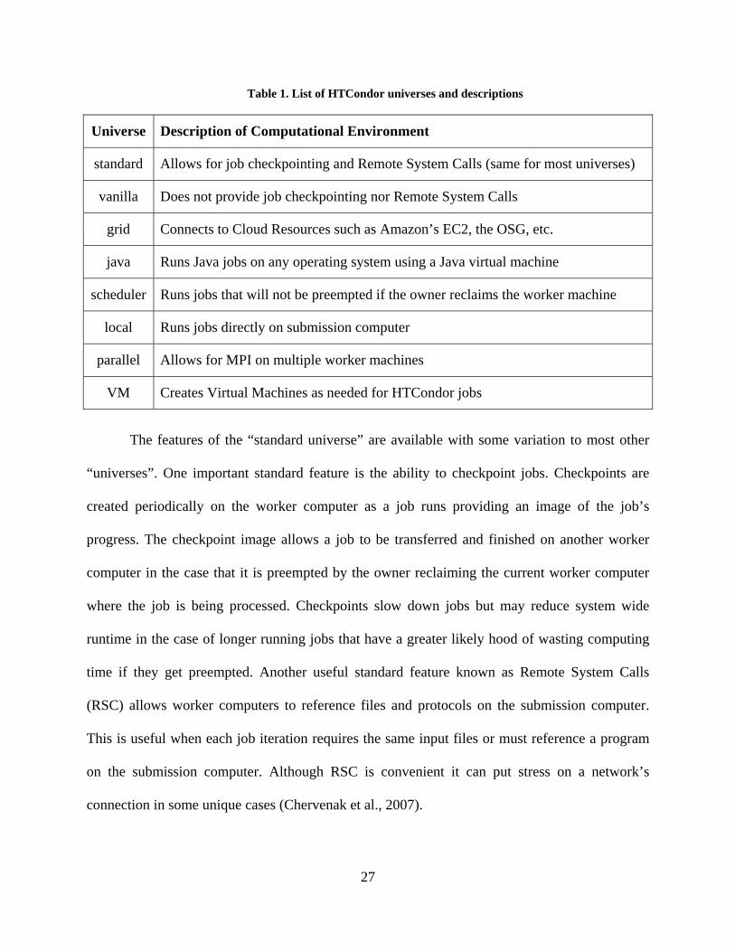
Table 1. List of HTCondor universes and descriptions

Universe Description of Computational Environment

standard Allows for job checkpointing and Remote System Calls (same for most universes)

vanilla Does not provide job checkpointing nor Remote System Calls

grid Connects to Cloud Resources such as Amazon’s EC2, the OSG, etc.

java Runs Java jobs on any operating system using a Java virtual machine

scheduler Runs jobs that will not be preempted if the owner reclaims the worker machine

local Runs jobs directly on submission computer

parallel Allows for MPI on multiple worker machines

VM Creates Virtual Machines as needed for HTCondor jobs

The features of the “standard universe” are available with some variation to most other

“universes”. One important standard feature is the ability to checkpoint jobs. Checkpoints are

created periodically on the worker computer as a job runs providing an image of the job’s

progress. The checkpoint image allows a job to be transferred and finished on another worker

computer in the case that it is preempted by the owner reclaiming the current worker computer

where the job is being processed. Checkpoints slow down jobs but may reduce system wide

runtime in the case of longer running jobs that have a greater likely hood of wasting computing

time if they get preempted. Another useful standard feature known as Remote System Calls

(RSC) allows worker computers to reference files and protocols on the submission computer.

This is useful when each job iteration requires the same input files or must reference a program

on the submission computer. Although RSC is convenient it can put stress on a network’s

connection in some unique cases (Chervenak et al., 2007).

28

I used the “vanilla universe” for this research because it ran fast for my specific job needs

and is simple to set up. The jobs that I tested stochastic simulations on complete in about 15

minutes which is relatively fast and have good chance of completing before preemption. I

sacrificed the option of having checkpoints to gain computational speed with my short jobs.

Also, due to the small (600 KB total) inputs required by my test models of GSSHA there was no

trouble copying them over from the submission computer to the receiving worker computer.

3.2 External HTCondor Resources

External resources may include supercomputer or cloud computing nodes as well as links

to other master computers and their HTCondor pool of processors. Providing this flexibility in

the system is a powerful feature of HTCondor because it allows users to combine and employ

several computing methods as desired.

3.2.1 Cloud Resources

It is also possible to include commercial cloud resources as part of an HTCondor pool.

This requires specific settings in the job script and configuration file of the master computer. In

the configuration file the cloud resource types and server locations must be explicitly identified

in the “GRID” variable so that the master computer knows where to look to match and send jobs.

The “Universe” or environment of the job must be set to “GRID” in the job script and its

“Grid_Resource” option must be set to the specific cloud resource that you wish to use. Also, an

optional variable can be set in the job script to set a price threshold for jobs sent to the cloud, so

that jobs will only be run if the price per central processing unit (CPU) for an hour falls below

the threshold. For example, if you were using Amazon’s Elastic Compute Cloud (EC2) you

29

could set the “ec2_spot_price” variable to “0.011” so that HTCondor would send jobs to the

cloud only if the cost per CPU hour was $0.011 or less. One problem with creating price

threshold for EC2 spot resources is that if the price per CPU hour goes above the threshold while

the job is still running it may be terminated before the jobs is finished. The spot resource setting

is another feature that makes HTCondor ideal for high throughput computing on a budget.

(Center for High Throughput Computing, 2013)

3.2.2 Supercomputing Resources

Supercomputer nodes are treated exactly like worker computers when connected to an

HTCondor pool. HTCondor would be installed on the HPC nodes to replace any previous

scheduling manager and they would become available in the master computer’s list of resources.

In the case of a pool of mixed HPC and desktop resources a user can have a job computed on a

certain selection of resources by designating “Class Ad” requirements. Class Ads are a record of

attributes that HTCondor keeps for each of its available resources (Thain et al., 2005). These

attributes include operating system type, processor size, IP address, and network name, among

others.

3.2.3 External HTCondor Pools

Other HTCondor pools can also be linked to the local pool as external resources. Jobs are

sent first to the local master computer and then any superfluous idle jobs will be sent to the

external pool if it has sufficient resources available that fit the job criteria. External HTCondor

pools can be linked together with the FLOCK_FROM and FLOCK_TO variables in the condor

configuration file on each master computer. A master computer may be set up to send jobs to an

30

external pool, while not receiving additional jobs from any external pools. To connect two

HTCondor pools they do not need to be on the same sub-network, but they must share a reliable

network connection. There are many examples of single HTCondor flocks that span several

countries and thousands of miles with reliable connections (Epema et al., 1996).

A prime example of how a flock of HTCondor pools can be a powerful resource was

created by Epema et al. (1996). This flock facilitated a connection to several separate pools in

five different countries that can be utilized by all its participants by submitting jobs to

HTCondor. One advantage of such a widespread system of linked computing resources it that as

the work day rolls to a close in one time zone it frees up massive amounts of computing

resources for other areas that are just beginning their work day. One disadvantage of have a large

flock of computing resources is that the overhead of communicating between pools may increase

job times (Chervenak et al., 2007).

3.3 GSSHA

In conjunction with the computational power of HTCondor this project used the Gridded

Surface Subsurface Hydrologic Analyst (GSSHA) model. The GSSHA model is a fully

distributed physics-based model that can predict runoff in a watershed (Downer, Ogden, & Byrd,

2008). Stochastic simulations done with GSSHA lend themselves very well to the high-

throughput computing environment because they requires a great number of completely

independent computations (Basney, Raman, & Livny, 1999).

To produce a stochastic simulation with a GSSHA model some of the input files much be

altered. The files that I focused on for this project where the mapping table (CMT) file, project

(PRJ) file, and the outlet hydrograph (OTL) file. The CMT file contains most of the important

31

physical parameters that could be stochastically models with BYU’s web applications (Downer

et al., 2008). The PRJ file is the file that the GSSHA executable uses to find and reference all of

the other input files including the CMT file. The OTL file is the GSSHA output file that contains

a list of times and discharge rates that make up a hydrograph. For my project I used the peak

discharge from the OTL file as my parameter of interest to determine statistical convergence.

Because I used the HTCondor the “vanilla universe” to test my scripts and complete

stochastic simulations with GSSHA I had to send the GSSHA executable file (gssha.exe) with

each job. If the GSSHA executable would have been located in the same directory on ever

worker computer I could have referenced it locally, but sense it was not in the same location and

because is small (900 KB) I copied if over with each job. Along with the executable, GSSHA

requires several input files that also had to be copied over to each worker computer using. To

copy files from one computer to another for a job in HTCondor they must be referenced in the

job script. As GSSHA runs it generates several output files, a few of which are large files that

were not needed in the statistical calculations. These larger, unnecessary outputs were deleted

from the executing worker computer before the job completed so to eliminate the time required

to copy them back to the submitting computer. Most universes in HTCondor use one processor

per job which is suits the version of GSSHA that I used in my tests. However, the parallel

universe has potential to utilize the message passing interface (MPI) that is available in a recent

release of GSSHA and distribute the jobs over multiple processors. This would reduce runtimes

on larger models.

32

3.4 Stochastic Simulations and Statistical Convergence

Stochastic simulations will be the most computationally intensive service of our CI-

WATER web applications, and therefore computing such simulations would potentially be a

bottle neck in our system. Using HTCondor helps us to optimize our potential computing

bottleneck and make our web application design more robust and useful. HTCondor will provide

the job queuing and submission engine for the back end of these web services. To perform

stochastic simulations we needed to find a computing interface that could schedule and distribute

hundreds of individual jobs. Stochastic computations are a perfect candidate for HTCondor

because they are considered to be “embarrassingly parallel”. This means that each stochastic job

is 100% independent of the other stochastic jobs, and therefore easily distributed among separate

processors. In my test runs of GSSHA I performed stochastic simulations with the overland

roughness parameters that are found in the CMT file. I assumed that the uncertainty of the

roughness value occurred according to a normal distribution with a certain standard deviation

about a mean value. Using Python I generated a random value for each roughness and rewrote

the CMT file. The new CMT file was then copied over with all of the original inputs and

GSSHA was run on HTCondor. The varied roughness values in the CMT file produced variation

in the outlet hydrograph or OTL file of the GSSHA model. I was then able to generate statistics

based on all of the different OTL files that represented the possibilities of discharge in a

watershed based on the uncertainty inherent in the overland roughness input parameter. This

same type of simulation could be reproduced for and input parameter or combination of

parameters for any GSSHA model.

An important part of running stochastic simulations efficiently with limited resources is

to testing for statistical convergence. In the context of a Monte Carlo simulation statistical

33

convergence is reached when we continue randomly sampling the solution space but the average

value of the model result of interest (peak discharge for example) ceases to change significantly.

Since the statistic that we are interested in has stopped changing more samples in the solution

space are not needed and we can stop the simulation. One of the Python scripts that I used to do

stochastic simulations with GSSHA required a specific number of iterations to perform, all of

which must run before statistics could be calculated on the whole job. The other Python script

calculated statistics during the job as each iteration completed. Using this method I was able to

monitor the last five changes to the average peak discharge for the whole job and once the

average of those changes fell below a set tolerance value I assumed statistical convergence had

been reached for the simulation and canceled the rest of the simulations in the HTCondor queue.

A sample graph of the change in average peak discharge per number of jobs completed is shown

in Figure 2 below.

O

from the

calculate

allows us

using the

jobs to

converge

Python s

final stoc

statistica

Once statistic

HTCondor

d statistics.

s to reduce w

ese Python s

run. The id

ence is achie

cript will te

chastic resul

l convergenc

Figure 2

cal converge

queue by th

Testing for s

wasted CPU

scripts and H

dea is to g

eved. If by ch

erminate nor

lts file. Figu

ce.

2. Stochastic co

ence was rea

he Python sc

statistical co

U usage and c

HTCondor th

uess high a

hance the us

rmally once

ure 3 shows

34

onvergence of

ached the rem

cript and a r

onvergence a

complete job

he user woul

and let the

ser does not

all of the sc

the logic em

f average peak

maining unn

results file w

and removin

bs faster. To

ld put a con

Python scr

guess a high

cheduled job

mployed by

k discharge

necessary job

was written

ng excess job

o start a stoc

servative gu

ript abort th

h enough nu

bs have run

the Python

bs were rem

summarizin

bs from the q

chastic simul

uess at how m

he process

umber of job

and still cre

script to ach

moved

ng the

queue

lation

many

once

s, the

eate a

hieve

35

Figure 3. Diagram of how statistical convergence is determined for this project

3.5 Using Python to Connect GSSHA and HTCondor

Python has been chosen as the interpreted language of choice for the CI-WATER project.

The web-based applications, database queries, and input/output tools are being constructed in

Python. To support consistency with the CI-WATER project, Python was the scripting language

used to interact with HTCondor as well as generate the varied inputs for GSSHA to create

stochastic simulations. The Python scripts that I developed have four purposes.

1. Make and organize a file structure that can dynamically manage inputs and outputs

for the jobs sent to and run on HTCondor.

2. Generate randomized GSSHA input files and HTCondor job and executable files in

their respective directories.

36

a. The Python script creates a job file that defines the environments of the

HTCondor job including which files the current job will need as inputs, how

many iterations of the job to put the queue, and how to handle the outputs

upon completion of the job.

b. The script also creates the executable file that HTCondor will use to run the

job on the receiving worker computer. For this application in a Windows

operating system this file is a batch script which simply starts another Python

script that randomizes the specified GSSHA inputs and then runs the GSSHA

model.

c. The CMT or mapping table file is an input file for GSSHA where most of the

physical parameters of a watershed are located. The Python script rewrites

this file from the calibrated GSSHA inputs and randomly selects new

parameter values within a normal distribution. For my tests I selected the

overland roughness parameter to vary randomly.

d. My Python script also makes alterations to the PRJ or project file. This

GSSHA file references all of the other inputs and therefore had to be

rewritten to include the correct path to the new CMT file.

3. Using the subprocess module in Python my scripts submit the job file to HTCondor

for processing as well as start the GSSHA model running on the receiving worker

computer. Having Python function as the middleware for starting various processes

and programs allows for a simpler user interactions with the system.

4. Another role that Python plays in these stochastic GSSHA simulations is that it

parses the results folder on the submission computer and generates statistics as

37

outputs are copied back from the worker computers through HTCondor. While the

Python script sniffs the results folder and processes new outputs that arrive it keeps a

running calculation of the average peak discharge from the outlet hydrograph that

GSSHA produces. If the average stops changing significantly then the Python script

considers the simulation to have reached statistical convergence and sends a

command to HTCondor to remove the remaining iterations of that specific job from

the queue. Testing for statistical convergence and removing superfluous jobs allows

us to use computing time more efficiently.

I developed and tested two methods for parallelizing GSSHA and running stochastic

simulations. The first let the randomization of the inputs be performed with in each job iteration

that ran on the worker computers and it used statistical convergence to cut the stochastically

simulation short if possible. The second method performed all of the input randomization on the

submission computer before the job was submitted to HTCondor and it simply executed a user

defined number of job iterations without statistical convergence.

The first method required two separate Python scripts called “sendOneRndCondor.py”

and “oneRndGSSHA.py”. The “sendOneRndCondor.py” script set up and submitted the

stochastic simulation to HTCondor from the submission computer. The “oneRndGSSHA.py”

script was submitted along with the job and produced the randomized CMT file and ran GSSHA

on the executing worker computers with the new input. A limitation of this method was that

Python was required on all of the worker computers to produce the random CMT file. A benefit

of this method was that it was more computationally efficient because it computed the stochastic

results as jobs finished and outputs returned from the queue. The “sendOneRndCondor.py” script

constantly parsed the results folder and generated a dynamic average peak discharge each time a

38

new OTL file was written back from HTCondor. It also calculated a convergence test value by

averaging the previous five changes to the average peak discharge and compared it to a the

convergence tolerance set by the user. Once the test value became less than the tolerance the

Python script considered statistical convergence to be reached and then removed the remaining

jobs from the queue and generated a final statistical results file. Figure 4, below, shows how the

Python scripts from the first method interact with HTCondor and GSSHA to efficiently generate

stochastic simulation. HTCondor acts as a link between the submission and worker computers by

following the job description in the job file.

Accepting ComputerSubmission Computer

Job Script

sendOneRndCondor.py

Results Folder

oneRndGSSHA.py

gssha.exe

GSSHA Inputs

GSSHA Inputs

gssha.exe

oneRndGSSHA.py

New GSSHA Inputs

Copy Over

Copy OverGSSHA Outputs

Run

RunBatch File

Batch File

SubmitJob Script

Figure 4. Python script interaction with HTCondor

39

The second method used one Python script called “multRndCondorGSSHA.py” which

created all of the randomized CMT files on the submission computer before submitting each job

iteration individually to HTCondor. This method was limited in that it did not test for statistical

convergence, but instead ran the exact number of jobs the user requested. One possible benefit of

this method it that is did not require the receiving worker computers to have Python installed on

them. The GSSHA executable was the only thing that had to be run on the receiving computers.

Once the last job finished and the final outputs were written back to the submission computer the

Python script generated a final results file. This method is less complicated than the first, but it

does not utilize HTCondor to its full potential nor does it use compute time as efficiently by

varying the number of job iterations that get completed based on statistical convergence.

Table 2 summarizes a comparison of the two methods that were developed to test

stochastic simulations of GSSHA on HTCondor. The comparisons are based on the four

functions of Python that were outlined as necessary for completing this project.

40

Table 2. Comparison of the two stochastic GSSHA simulation methods

Function Method 1 Method 2

Manage File Structure

Creates a new results folder on the submission computer

Creates a new results folder on the submission computer

Creates one job that resides with all of its inputs and outputs directly in the results folder.

Creates a new folder for each job’s inputs and outputs within the results folder

Write Files Writes one job file that produces multiple iterations

Writes a job file for each job iteration

Writes one batch executable referenced by every job iteration

Writes a batch executable for each job iteration

Writes a new project (prj) file for each job iteration on the receiving computer

Writes a new project file for each job iteration on the submission computer

Writes a new mapping table (cmt) file for each job iteration on the receiving computer

Writes a new mapping table file for each job iteration on the submission computer

Submit Jobs to HTCondor

Single job script queues multiple jobs in HTCondor

Each job script queues one job in HTCondor

Sends original GSSHA files with job to receiving computers

Sends original and altered GSSHA files with job to receiving computers

Sends gssha.exe with job Sends gssha.exe with job Sends a second Python script with job to receiving computers

Does not send any Python scripts with job to receiving computer

Batch executable calls the second python script on the receiving computer

Batch executable calls the gssha.exe directly on the receiving computer

Parse Outputs-Generate Statistics

Parses outputs as they are written back to the submission computer

Only parses outputs after all job iterations have completed

Calculates statistics continually and terminates remaining job iterations if statistics converge

Calculates statistics once after all job iterations have completed

41

4 CASE STUDY

In developing my Python scripts for this project I began with very simplistic GSSHA

models that had few inputs and only required a minute or so to run. Once the scripts were ready I

tested them on models of various sizes and configurations to be sure that the scripts were robust

enough to ingest any GSSHA model that I had encountered. For testing stochastic simulations

with the finalized scripts I used the long term advanced groundwater model from the GSSHA

tutorials. This particular GSSHA model had six precipitation events and used hydro-

meteorological (HMET) data to simulate a two week period. This GSSHA model took an

average of 14 minutes to run on a normal desktop computer using version 4.0 of the GSSHA

executable which does not support MPI. To run 150 instances of this model in series it would

take roughly 2,100 minutes or 35 hours.

Because of the nature of HTCondor each stochastic simulation ran on a different number

of processors ranging from about 80 to 140. As expected, with about 100 times the

computational power of normal circumstances I was able to essentially reduce the runtime by

factor of 100. Figure 5 shows the relationship of the time in minutes that it took several

stochastic simulations to complete versus the number of iterations required to reach statistical

convergence. This plot shows a rough linear relationship between simulation run time and

iterations number. It is difficult to confirm this linear relationship, however, due to the varied

42

number of available computing resources for each simulation. More testing would be required to

establish a concrete relationship between the runtime and number of jobs that may exist on our

specific HTCondor pool.

Figure 5. Plot of the time it took to complete certain numbers of iterations

Using a convergence tolerance of 0.001 this model required from 15.9 to 33.3 minutes to

run between 115 and 185 jobs. Below, Figure 6 shows four graphs of different stochastic

simulations that were run on the HTCondor pool at BYU using that tolerance. The number of

processors available for these simulations fluctuated between 80 and 140 processors and the

average runtime was about 22 minutes. Using the convergence tolerance of 0.001 the average

peak discharge ranged from 9.54 to 9.72 cms.

R² = 0.9382

0

20

40

60

80

100

120

140

0 200 400 600 800 1000 1200

Time [min]

Number of job iterations completed

43

The spread of average peak discharge values obtained from a tolerance of 0.001seems too

wide to demonstrate true convergence so I ran simulaitons with a taolerance of 0.0001. Figure 7

shows the graph of statistical convergence for one of the stochastic simulations generated with a

tolerance of 0.0001. To make sure that I was going to run enough jobs to achieve convergence

with this tolerance I sent 10,000 job iterations to HTCondor for processing. This simulation

shows how using convergence can save on compute time because only 1,181 iterations had to

complete to achieve the tolerance that I was aiming for. About 8,800 jobs were removed from

HTCondor before they ever had to run, which saved potentially hundreds of CPU hours from

‐5

‐4

‐3

‐2

‐1

0

1

2

3

0 50 100 150 200

Chan

ge in

 average

 peak discharge

Number of job iterations completed

‐5

‐4

‐3

‐2

‐1

0

1

2

3

0 50 100 150 200

Chan

ge is average

 peak discharge

Nubmer of job iterations copleted

‐5

‐4

‐3

‐2

‐1

0

1

2

3

0 50 100 150 200

Chan

ge in

 average

 peak discharge

Number of job iterations completed

‐5

‐4

‐3

‐2

‐1

0

1

2

3

0 50 100 150 200

Chan

ge in

 aberage

 peak discharge

Number of job interations completed

A B

C D

Figure 6. A-D are graphs of statistical convergence for a tolerance of 0.001

44

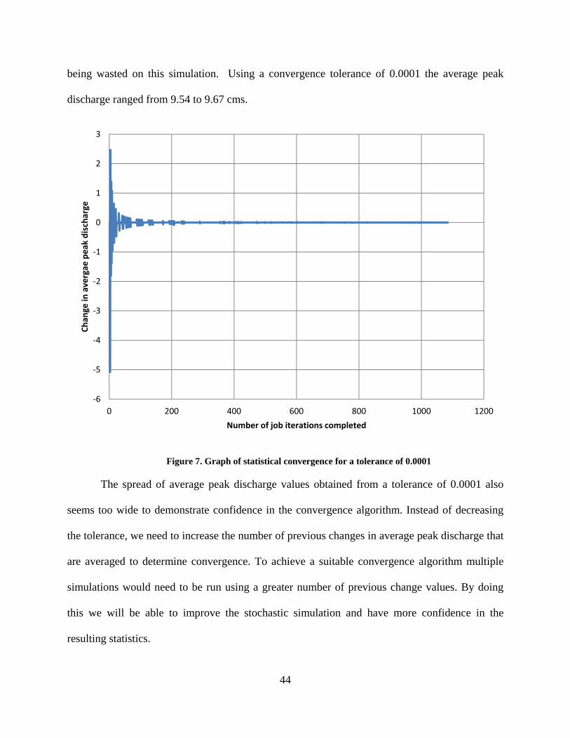
being wasted on this simulation. Using a convergence tolerance of 0.0001 the average peak

discharge ranged from 9.54 to 9.67 cms.

Figure 7. Graph of statistical convergence for a tolerance of 0.0001

The spread of average peak discharge values obtained from a tolerance of 0.0001 also

seems too wide to demonstrate confidence in the convergence algorithm. Instead of decreasing

the tolerance, we need to increase the number of previous changes in average peak discharge that

are averaged to determine convergence. To achieve a suitable convergence algorithm multiple

simulations would need to be run using a greater number of previous change values. By doing

this we will be able to improve the stochastic simulation and have more confidence in the

resulting statistics.

‐6

‐5

‐4

‐3

‐2

‐1

0

1

2

3

0 200 400 600 800 1000 1200

Chan

ge in

 avergae

 peak discharge

Number of job iterations completed

45

5 CONCLUSIONS

The conclusions from this project are as follows:

5.1 HTCondor

HTCondor is a useful computing resource for running stochastic simulations. One of the

main benefits of HTCondor is that it works with both internal and external computing resources.

HTCondor provides a robust queuing environment that has been well developed since 1984. New

research is being conducted with HTCondor every year and it continues to gain more and more

functionality while maintaining its original purpose.

HTCondor is well developed scheduling software that contains much of the functionality

that researchers associated with the CI-WATER project need to process the jobs that will be

generated from web-based hydrologic tools. It has enough computing power to handle intense

stochastic simulations and the simplicity to manage single computational jobs as well. This

project also serves as a successful case study of how two ways Python might be utilized to

automate a great deal of HTCondor’s functionality. Using the scripts developed in this project as

a pattern, HTCondor could be used for many other applications besides GSSHA jobs.

46

5.2 Mary Lou

BYU’s supercomputer, Mary Lou, is a powerful collection of HPC clusters that is useful

for many computational applications. For a majority of the computational needs for our web

applications , however, we have found that the environment that HTCondor provides is much

more suited to our research. The supercomputer does not have the ideal operating system nor the

Python environment for the applications that we would like to support with our hydrologic web

interfaces which include options for stochastic simulations. Also, the supercomputer’s queue is

completely controlled by the BYU’s Fulton Supercomputing Lab (FSL), which makes it difficult

to connect it to our web applications for quick turnaround of jobs.

Supercomputing with the FSL produces slower job turnaround than HTCondor because,

as researchers, we share the super computer with dozens of other departments. We have to

compete for run time on the super computer, and as we use more time than other research

accounts our priority falls in comparison. A single job that we send to Mary Lou can take hours

to reach the queue while similar jobs only have to wait 30 minutes at most with HTCondor.

5.3 Amazon Cloud

Commercial cloud computing services are innovative and can be very useful, but because

of the cost involved they are probably best-suited as a flexible extension of HTCondor. In this

way cloud resources could provide vast amounts of computational power on short notice in the

case of a fluctuation in computational need while HTCondor accessing local computers would

serve as the main source of computational power for our web applications a majority of the time.

47

5.4 Future Work

With the successful completion of this preliminary assessment of HTCondor’s potential

there are several tasks that will naturally follow. First, more testing could be done using different

HTCondor universes to provide even more flexibility and stronger fit for various types of jobs.

Also, the Texas Water Mapper could be connected to the HTCondor pool of resources to begin

testing its computational performance on an existing web-based application. Tests need to be

conducted on the ease and reliability of connecting to and running jobs on cloud resources based

on cost per CPU hour. The Python code for this project could be rewritten to be object oriented

so that it fits in with CI-WATER’s coding standards and provides a more general coding model

for interfacing with HTCondor.

48

REFERENCES

Basney, Jim, Raman, Rajesh, & Livny, Miron. (1999). High throughput monte carlo. Paper presented at the Proceedings of the Ninth SIAM Conference on Parallel Processing for Scientific Computing.

Bradley, D, St Clair, T, Farrellee, M, Guo, Z, Livny, M, Sfiligoi, I, & Tannenbaum, T. (2011). An update on the scalability limits of the condor batch system. Paper presented at the Journal of Physics: Conference Series.

Center for High Throughput Computing, University of Wisconsin-Madison. (2013). HTCondorTM Version 7.8.8 Manual. from http://research.cs.wisc.edu/htcondor/manual/v7.8/ref.html

Chervenak, Ann, Deelman, Ewa, Livny, Miron, Su, Mei-Hui, Schuler, Rob, Bharathi, Shishir, . . . Vahi, Karan. (2007). Data placement for scientific applications in distributed environments. Paper presented at the Grid Computing, 2007 8th IEEE/ACM International Conference on.

Couvares, Peter, Kosar, Tevfik, Roy, Alain, Weber, Jeff, & Wenger, Kent. (2007). Workflow Management in Condor. In I. Taylor, E. Deelman, D. Gannon & M. Shields (Eds.), Workflows for e-Science (pp. 357-375): Springer London.

Downer, Charles W, Ogden, Fred L, & Byrd, A.R. (2008). Gridded Surface Subsurface Hydrologic Analysis Version 4.0 for WMS 8.1 GSSHAWIKI User’s Manual: ERDC Technical Report, Engineer Research and Development Center, Vicksburg, Mississippi.

Epema, D. H. J., Livny, M., van Dantzig, R., Evers, X., & Pruyne, J. (1996). A worldwide flock of Condors: Load sharing among workstation clusters. Future Generation Computer Systems, 12(1), 53-65. doi: http://dx.doi.org/10.1016/0167-739X(95)00035-Q

Goux, Jean-Pierre, Linderoth, Jeff, Yoder, Michael, & Goux, Jean-pierre. (2000). Metacomputing and the master-worker paradigm. Paper presented at the Preprint MCS/ANL-P792-0200, Mathematics and Computer Science Division, Argonne National Laboratory, Argonne.

Litzkow, Mike, & Livny, Miron. (1990). Experience with the condor distributed batch system. Paper presented at the Experimental Distributed Systems, 1990. Proceedings., IEEE Workshop on.

Thain, Douglas, Tannenbaum, Todd, & Livny, Miron. (2005). Distributed computing in practice: the Condor experience. Concurrency and Computation: Practice and Experience, 17(2-4), 323-356. doi: 10.1002/cpe.938

Thain, Douglas, Tannenbaum, Todd, & Livny, Miron. (2006). How to measure a large open‐source distributed system. Concurrency and Computation: Practice and Experience, 18(15), 1989-2019.

49

Wright, Derek. (2001). Cheap cycles from the desktop to the dedicated cluster: combining opportunistic and dedicated scheduling with Condor. Paper presented at the Conference on Linux clusters: the HPC revolution.

50

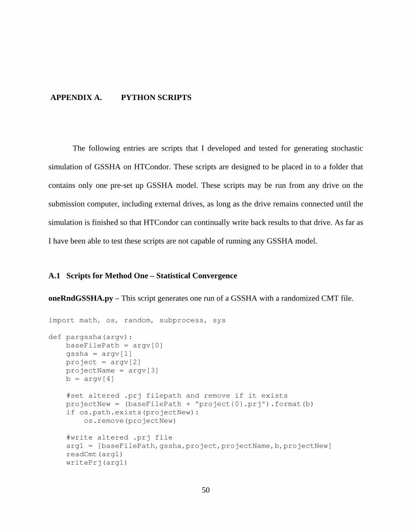
APPENDIX A. PYTHON SCRIPTS

The following entries are scripts that I developed and tested for generating stochastic

simulation of GSSHA on HTCondor. These scripts are designed to be placed in to a folder that

contains only one pre-set up GSSHA model. These scripts may be run from any drive on the

submission computer, including external drives, as long as the drive remains connected until the

simulation is finished so that HTCondor can continually write back results to that drive. As far as

I have been able to test these scripts are not capable of running any GSSHA model.

A.1 Scripts for Method One – Statistical Convergence

oneRndGSSHA.py – This script generates one run of a GSSHA with a randomized CMT file.

import math, os, random, subprocess, sys def pargssha(argv): baseFilePath = argv[0] gssha = argv[1] project = argv[2] projectName = argv[3] b = argv[4] #set altered .prj filepath and remove if it exists projectNew = (baseFilePath + "project{0}.prj").format(b) if os.path.exists(projectNew): os.remove(projectNew) #write altered .prj file arg1 = [baseFilePath,gssha,project,projectName,b,projectNew] readCmt(arg1) writePrj(arg1)

51

subprocess.call([gssha, projectNew]) def writePrj(argv): baseFilePath = argv[0] project = argv[2] b = argv[4] projectNew = argv[5] for file in os.listdir(baseFilePath): if file.endswith('.prj'): project = baseFilePath + file newPrjFile = open(projectNew, 'a') for line in open(project): if line.split()[0] == "SUMMARY": lineBy =line.strip().split() newPrjFile.write((lineBy[0] + "\t\t\t\t\t " + '"' + "project{0}.sum" + '"\n').format(b)) elif line.split()[0] == "OUTLET_HYDRO": lineBy =line.strip().split() newPrjFile.write((lineBy[0] + "\t\t\t " + '"' + "project{0}.otl" + '"\n').format(b)) elif line.split()[0] == "MAPPING_TABLE": lineBy =line.strip().split() newPrjFile.write((lineBy[0] + "\t\t\t " + '"' + "project{0}.cmt" + '"\n').format(b)) else: newPrjFile.write(line) newPrjFile.close() def readCmt(argv): baseFilePath = argv[0] b = argv[4] for file in os.listdir(baseFilePath): if file.endswith('.cmt'): cmtFilePath = baseFilePath + file newCmt = (baseFilePath + "project{0}.cmt").format(b) cmt = open(cmtFilePath) new = open(newCmt, 'a') #this creates a new file nextLine = cmt.readline() new.write(nextLine) nextLine = cmt.readline() while nextLine.split()[0] == "INDEX_MAP": new.write(nextLine) nextLine = cmt.readline()

52

new.write(nextLine) nextLine = cmt.readline() numIDs = int(nextLine.split()[-1]) new.write(nextLine) nextLine = cmt.readline() new.write(nextLine) for i in range(0,numIDs): nextLine = cmt.readline() lineBy = nextLine.split() mean = float(lineBy[-1]) min1 = mean*0.8 max1 = mean*1.2 stdev = (max1-min1)/6 num = normalDist(mean,stdev,min1,max1) repLine =nextLine.replace(lineBy[-1], str(num)[:7]) new.write(repLine) for i in range(0,500): nextLine = cmt.readline() new.write(nextLine) new.close() def normalDist(mean,stdev,min1,max1): x= (min1-5.0) while max1 > x < min1: x = gauss()*stdev + mean return x def gauss(): fac = 0.0 r = 1.5 V1 = 0.0 V2 = 0.0 rnd = random.random while r>=1: V1 = 2*rnd() - 1 V2 = 2*rnd() - 1 r = V1**2 + V2**2 fac =(-2*math.log(r)/r)**(1/2.0) gauss = V2*fac return gauss #set basepath baseFilePath = os.getcwd() + "\\"

53

#set gssha.exe path gssha = baseFilePath + "gssha.exe" #set main .prj file path allFiles = os.listdir(baseFilePath) for file in allFiles: if file.endswith('.prj'): project = baseFilePath + file projectName = file.split(".")[0] b = random.randrange(0,1000000000) arg1 = [baseFilePath,gssha,project,projectName,b] pargssha(arg1)

sendOneRndCondor.py – Sends multiple instances of “oneRndGSSHA.py to HTCondor to be

processed and parses the outputs from those jobs to generate statistics on peak discharge. This

script terminates the simulations based on statistical convergence.

import os, subprocess, time, re def parseResults(resultFilePath,numRuns): numRuns = float(numRuns) maxPeak = [0.0,0.0] minPeak = [100000000000000000000000000000000.0,0.0] sumPeak = [0.0,0.0] sqrsumPeak = [0.0,0.0] avePeak = [0.0,0.0] stdPeak = [0.0,0.0] varPeak = [0.0,0.0] listPeak = [] listTime = [] for file in os.listdir(resultFilePath): if file.endswith('.otl'): oltFilePath = resultFilePath + file peak = extractPeakFlow(oltFilePath) sumPeak[0] = sumPeak[0] + peak[0] sumPeak[1] = sumPeak[1] + peak[1] listPeak.append(peak[0]) listTime.append(peak[1]) if peak[0] > maxPeak[0]: maxPeak = peak elif peak[0] < minPeak[0]: minPeak = peak avePeak[0] = sumPeak[0]/numRuns avePeak[1] = sumPeak[1]/numRuns

54

for i in range(0,len(listPeak)): varPeak[0]= varPeak[0] + ((listPeak[i]-avePeak[0])**2) varPeak[1]= varPeak[1] + ((listTime[i]-avePeak[1])**2) stdPeak[0] = (varPeak[0]/numRuns)**(0.5) stdPeak[1] = (varPeak[1]/numRuns)**(0.5) stats = [avePeak,stdPeak] return stats def extractPeakFlow(otlFilePath): openOtl = open(otlFilePath) peak = [0.0,0.0] flow = 0.0 for line in openOtl: lineBy = line.split() flow = float(lineBy[1]) if flow > peak[0]: peak[0] = flow # include the time for comparison peak[1] = float(lineBy[0]) return peak def quitCondor(jobNum): #This will only remove the current job subprocess.call(["condor_rm",jobNum]) def getIdleJobNum(resulsFilePath, jobQcommand): subprocess.call([jobQcommand]) for jobfile in os.listdir(resulsFilePath): if jobfile == "jobQ.out": for line in open(resulsFilePath+jobfile): if 'jobs' in line: idleJobNum = int(re.search('(\d+) jobs',line).group(0).split()[0]) else: idleJobNum = 1 return idleJobNum def fileCollector(resultFilePath,numJobs): resultFileList = set() oldStats = 0.0 delta = [] oldNumFiles = len(resultFileList) eps = 1 #this pulls the job number (cluster #) of the job out of the submit.out file for jobfile in os.listdir(resultFilePath): if jobfile == "submit.out": for line in open(resultFilePath+jobfile): if 'cluster' in line:

55

jobNum = re.search('cluster (\d+)',line).group(0).split()[1] for jobfile in os.listdir(resultFilePath): if jobfile.endswith(".job"): for line in open(resultFilePath+jobfile): if 'Queue' in line: qNum = int(re.search('Queue (\d+)',line).group(0).split()[1]) """drive = resultFilePath.split(':')[0] jobQcommand = resultFilePath + "jobQ.bat" file = open(jobQcommand, 'a') file.write(drive + ": \n") file.write("cd " + resultFilePath + "\n") file.write("condor_q " + jobNum + " > jobQ.out\n") file.close()""" #test for convergnece and then remove the remaining jobs from HTCondor while eps > 0.0001: resultsFiles = os.listdir(resultFilePath) for file in resultsFiles: if file.endswith('.otl'): resultFileList.add(file) numFiles = len(resultFileList) if numFiles == oldNumFiles: #if you didnt send enough jobs for convergence this should get you out of the loop if numFiles == numJobs: eps = 0 else: pass elif oldNumFiles < numFiles: newStats = parseResults(resultFilePath,numFiles) delta.append((oldStats-newStats[0][0])) if len(delta) > 5: eps = (abs(delta[-1])+abs(delta[-2])+abs(delta[-3])+abs(delta[-4])+abs(delta[-5]))/5 oldStats = newStats[0][0] oldNumFiles = numFiles quitCondor(jobNum) results = [newStats,delta,numFiles,eps] return results def pargssha(baseFilePath,resultFilePath,b,numJobs): #write job, exe, and submit files fileList = fileFinder(baseFilePath) writeJob(resultFilePath,b,numJobs,fileList)

56

writeExe(resultFilePath,b) writeSubmit(resultFilePath,b) submitCommand = resultFilePath + "submit.bat" subprocess.call([submitCommand]) def writeJob(resultFilePath,b,numJobs,fileList): pr="project%s." %(b) newJobFile = resultFilePath + pr + "job" fileStr = "" file = open(newJobFile, 'a') file.write("Universe = vanilla\n") file.write(("Executable = {0}bat\n").format(pr)) file.write('Requirements = Arch == "X86_64" && OpSys == "WINDOWS"\n') file.write("Request_Memory = 1200 Mb\n") file.write(("Log = {0}log.txt\n").format(pr)) file.write(("Output = {0}out.txt\n").format(pr)) file.write(("Error = {0}err.txt\n").format(pr)) file.write("transfer_executable = TRUE\n") file.write("transfer_input_files = " + fileList[0]) for i in range(1,len(fileList)): fileStr = fileStr + ","+ fileList[i] file.write(fileStr + "\n") file.write("should_transfer_files = YES\n") file.write("when_to_transfer_output = ON_EXIT_OR_EVICT\n") file.write(("Queue {0} \n").format(numJobs)) file.close() def writeExe(resultFilePath,b): newExe = resultFilePath + "project%i.bat" %(b) file = open(newExe, 'a') file.write("C:\Python26\ArcGIS10.0\python.exe oneRndGSSHA.py > cmdout.txt\n") file.close() def writeSubmit(resultFilePath,b): drive = resultFilePath.split(':')[0] # this allows the jobs to be sent from a thumb drive newBat = resultFilePath + "submit.bat" file = open(newBat, 'a') file.write(drive + ": \n") file.write("cd " + resultFilePath + "\n")

57

file.write(("condor_submit " + resultFilePath + "project{0}.job > submit.out\n").format(b)) file.close() def fileFinder(baseFilePath): fileList = [] files = os.listdir(baseFilePath) for file in files: if file.endswith('.prj'): project = baseFilePath + file projectName = file.split(".")[0] for file in files: if file.startswith(projectName): if file.endswith(".ohl") or file.endswith(".rec") or file.endswith(".gmh") or file.endswith(".dep"): pass else: fileList.append(baseFilePath + file) elif file.endswith(".idx"): fileList.append(baseFilePath + file) elif file.endswith("gssha.exe"): fileList.append(baseFilePath + file) elif file.endswith("oneRndGSSHA.py"): fileList.append(baseFilePath + file) elif file.startswith("HMET"): fileList.append(baseFilePath + file) return fileList def main(): t1 = time.clock() #set basepath baseFilePath = os.getcwd() + "\\" #set and clear results folder resultFilePath = baseFilePath + "Results1\\" b = 2 while os.path.exists(resultFilePath): resultFilePath = (baseFilePath + "Results{0}\\").format(b) b = b + 1 b=b-1 #"b" is the number of the current Results folder #Make current Results path if not os.path.exists(resultFilePath): os.makedirs(resultFilePath) numJobs = 500 pargssha(baseFilePath,resultFilePath,b, numJobs)

58

results = fileCollector(resultFilePath,numJobs) dt = (time.clock()) -t1 resultsOutFile = open((resultFilePath + "result{0}.out").format(b),'a') resultsOutFile.write("main Results = \n") for i in range(0,len(results)): resultsOutFile.write(str(results[i]) + "\n") resultsOutFile.write(("Finished in {0} seconds.\n").format(int(round(dt,0)))) resultsOutFile.close csv = open((resultFilePath + "result{0}.csv").format(b),'a') for i in range(0,len(results[1])): csv.write(str(i+1) + "," + str(results[1][i]) + "\n") csv.close() if __name__ == '__main__': main()

A.2 Scripts for Method Two – Static Number of Jobs

multRndCondorGSSHA.py – This script runs a set number of randomized GSSHA models on

HTCondor and parses the outputs to generate a statistical results file. All of the randomized CMT

files are created on the submission computer prior to submitting jobs to HTCondor.

import math, os, random, subprocess, sys, threading, time t1 = time.clock() def pargssha(argv): baseFilePath = argv[0] project = argv[1] projectName = argv[2] stuff = argv[3] b = argv[4] i = argv[5] gssha = argv[6] resultFilePath = argv[7] run = argv[8] cmt = argv[9] fileList = argv[10] #create a new work folder to copy altered .prj file into

59

newPath = (resultFilePath + "NewGSSHAfolder{0}_{1}\\").format(b,i) if not os.path.exists(newPath): os.makedirs(newPath) #set altered .prj filepath and remove if it exists projectNew = (newPath + "project{0}_{1}.prj").format(b,i) if os.path.exists(projectNew): os.remove(projectNew) rain = "" #write altered .prj file arg1 = [baseFilePath,newPath,project,projectNew,projectName,stuff,rain,b,i,gssha,resultFilePath,run,cmt,fileList] readCmt(arg1) writePrj(arg1) writeJob(arg1) writeExe(arg1) writeSubmit(arg1) submitCommand = newPath + "submit.bat" subprocess.call([submitCommand]) def writeJob(argv): baseFilePath = argv[0] newPath = argv[1] projectName = argv[4] b = argv[7] i = argv[8] gssha = argv[9] pr="project%i_%i." %(b,i) newJobFile = newPath + pr + "job" fileStr = "" file = open(newJobFile, 'a') file.write("Universe = vanilla\n") file.write(("Executable = {1}bat\n").format(newPath,pr)) file.write('Requirements = Arch == "X86_64" && OpSys == "WINDOWS"\n') file.write(("Request_Memory = 1200 Mb\n").format(pr)) file.write(("Log = {0}log.txt\n").format(pr)) file.write(("Output = {0}out.txt\n").format(pr)) file.write(("Error = {0}err.txt\n").format(pr)) file.write("transfer_executable = TRUE\n") file.write(("transfer_input_files = " + gssha + ",{0}prj,{0}cmt").format(pr)) for i in range(0,len(fileList)): fileStr = fileStr + ","+ fileList[i] file.write(fileStr + "\n")

60

file.write("should_transfer_files = YES\n") file.write("when_to_transfer_output = ON_EXIT_OR_EVICT\n") file.write("Queue\n") file.close() def writeExe(argv): newPath = argv[1] projectName = argv[4] b = argv[7] i = argv[8] pr="project%i_%i." %(b,i) newExe = newPath + pr + "bat" file = open(newExe, 'a') file.write(("gssha.exe {0}prj > cmdout.txt\n").format(pr)) file.write(("del {0}.dep /F /Q\n").format(projectName)) file.write(("del {0}.rec /F /Q\n").format(projectName)) file.write(("del {0}.ghm /F /Q\n").format(projectName)) file.write("del maskmap /F /Q\n") #file.write("del out_time.out /F /Q\n") file.close() def writeSubmit(argv): newPath = argv[1] b = argv[7] i = argv[8] drive = newPath.split(':')[0] newBat = newPath + "submit.bat" file = open(newBat, 'a') file.write(drive + ": \n") file.write("cd " + newPath + "\n") file.write(("condor_submit " + newPath + "project{0}_{1}.job\n").format(b,i)) file.close() def writePrj(argv): baseFilePath = argv[0] newPath = argv[1] project = argv[2] projectNew = argv[3] projectName = argv[4] stuff = argv[5] rain =argv[6] b = argv[7] i = argv[8] idx = argv[13] for file in os.listdir(baseFilePath): if file.endswith('.prj'): project = baseFilePath + file

61

newPrjFile = open(projectNew, 'a') for line in open(project): if line.split()[0] == "SUMMARY": lineBy =line.strip().split() newPrjFile.write((lineBy[0] + "\t\t\t\t\t " + '"' + "project{0}_{1}.sum" + '"\n').format(b,i)) elif line.split()[0] == "OUTLET_HYDRO": lineBy =line.strip().split() newPrjFile.write((lineBy[0] + "\t\t\t " + '"' + "project{0}_{1}.otl" + '"\n').format(b,i)) elif line.split()[0] == "MAPPING_TABLE": lineBy =line.strip().split() newPrjFile.write((lineBy[0] + "\t\t\t " + '"' + "project{0}_{1}.cmt" + '"\n').format(b,i)) else: newPrjFile.write(line) newPrjFile.close() def readCmt(argv): baseFilePath = argv[0] newPath = argv[1] b = argv[7] i = argv[8] for file in os.listdir(baseFilePath): if file.endswith('.cmt'): cmtFilePath = baseFilePath + file newCmt = (newPath + "project{0}_{1}.cmt").format(b,i) cmt = open(cmtFilePath) new = open(newCmt, 'a') #this creates a new file nextLine = cmt.readline() new.write(nextLine) nextLine = cmt.readline() while nextLine.split()[0] == "INDEX_MAP": new.write(nextLine) nextLine = cmt.readline() new.write(nextLine) nextLine = cmt.readline() numIDs = int(nextLine.split()[-1]) new.write(nextLine) nextLine = cmt.readline() new.write(nextLine) for i in range(0,numIDs): nextLine = cmt.readline()

62

lineBy = nextLine.split() mean = float(lineBy[-1]) min1 = mean*0.8 max1 = mean*1.2 stdev = (max1-min1)/6 num = normalDist(mean,stdev,min1,max1) repLine =nextLine.replace(lineBy[-1], str(num)[:7]) new.write(repLine) for i in range(0,500): nextLine = cmt.readline() new.write(nextLine) new.close() def normalDist(mean,stdev,min1,max1): x= (min1-5.0) while max1 > x < min1: x = gauss()*stdev + mean return x def gauss(): fac = 0.0 r = 1.5 V1 = 0.0 V2 = 0.0 rnd = random.random while r>=1: V1 = 2*rnd() - 1 V2 = 2*rnd() - 1 r = V1**2 + V2**2 fac =(-2*math.log(r)/r)**(1/2.0) gauss = V2*fac return gauss def parseResults(path,numRuns,b,timeSum): resultFilePath = path numRuns = float(numRuns) b=b timeSum = timeSum openResultsSum = open((resultFilePath + "ResultSummary%i.txt" %b), 'a') maxPeak = [0.0,0.0] minPeak = [100000000000000000000000000000000.0,0.0] sumPeak = [0.0,0.0] sqrsumPeak = [0.0,0.0] avePeak = [0.0,0.0]

63

stdPeak = [0.0,0.0] varPeak = [0.0,0.0] listPeak = [] listTime = [] for dir in os.listdir(resultFilePath): currentFolder = resultFilePath + dir + "/" if os.path.isdir(currentFolder): for file in os.listdir(currentFolder): if file.endswith('.sum'): sumFilePath = currentFolder + file elif file.endswith('.otl'): oltFilePath = currentFolder + file peak = extractPeakFlow(oltFilePath) sumPeak[0] = sumPeak[0] + peak[0] sumPeak[1] = sumPeak[1] + peak[1] listPeak.append(peak[0]) listTime.append(peak[1]) if peak[0] > maxPeak[0]: maxPeak = peak elif peak[0] < minPeak[0]: minPeak = peak avePeak[0] = sumPeak[0]/numRuns avePeak[1] = sumPeak[1]/numRuns for i in range(0,len(listPeak)): varPeak[0]= varPeak[0] + ((listPeak[i]-avePeak[0])**2) varPeak[1]= varPeak[1] + ((listTime[i]-avePeak[1])**2) stdPeak[0] = (varPeak[0]/numRuns)**(0.5) stdPeak[1] = (varPeak[1]/numRuns)**(0.5) openResultsSum.write("MaxPeak Discharge = %f @ Time = %f\n" %(maxPeak[0],maxPeak[1])) openResultsSum.write("MinPeak Discharge = %f @ Time = %f\n" %(minPeak[0],minPeak[1])) openResultsSum.write("AvePeak Discharge = %f AveTime to Peak = %f\n" %(avePeak[0],avePeak[1])) openResultsSum.write("StDevPeak Discharge = %f StDevTime to Peak = %f\n" %(stdPeak[0],stdPeak[1])) openResultsSum.write(timeSum + "\n") openResultsSum.close() def extractPeakFlow(path): otlFilePath = path openOtl = open(otlFilePath) peak = [0.0,0.0] flow = 0.0 for line in openOtl: lineBy = line.split() flow = float(lineBy[1]) if flow > peak[0]:

64

peak[0] = flow # include the time for comparison peak[1] = float(lineBy[0]) return peak def fileFinder(baseFilePath): baseFilePath = baseFilePath fileList = [] files = os.listdir(baseFilePath) for file in files: if file.startswith(projectName): if file.endswith('.prj') or file.endswith(".cmt") or file.endswith(".ohl") or file.endswith(".rec") or file.endswith(".gmh") : pass else: fileList.append(baseFilePath + file) elif file.endswith(".idx"): fileList.append(baseFilePath + file) elif file.startswith("HMET"): fileList.append(baseFilePath + file) return fileList #set basepath baseFilePath = os.path.split( sys.argv[0] )[0] + "\\" print baseFilePath #set and clear results folder resultFilePath = baseFilePath + "Results1\\" b = 2 while os.path.exists(resultFilePath): resultFilePath = (baseFilePath + "Results{0}\\").format(b) b = b + 1 b=b-1 #"b" is the number of the current Results folder #Make current Results path if not os.path.exists(resultFilePath): os.makedirs(resultFilePath) #set gssha.exe path gssha = baseFilePath + "gssha.exe" print "The path to gssha.exe is " + gssha #set main .prj, .cmt, and .idx file paths project = "" allFiles = os.listdir(baseFilePath) for file in allFiles: if file.endswith('.prj'): projectName = file.split(".")[0] cmt = ""

65

fileList = fileFinder(baseFilePath) numRuns = 100 run = numRuns + 1 # run-1 is the number of theads that will be generated for i in range(1, run): print "Processing Project%i_%i..." %(b,i) #set variable to look for in main .prj file stuff = "RAIN_INTENSITY" arg1 = [baseFilePath,project,projectName,stuff,b,i,gssha,resultFilePath,run,cmt,fileList] #create thread "i" and run gssha model thread = threading.Thread(target=pargssha, args=[arg1]) thread.start() for i in range(0,1000000): pass thread.join() for i in range(1,run): checkFile = (resultFilePath + "NewGSSHAfolder{0}_{1}/project{0}_{1}.sum").format(b,i) while not os.path.exists(checkFile): pass print "WORKING..." dt = (time.clock()) -t1 timeSum = ("Finished {0} Projects in {1} seconds").format(i,int(round(dt,0))) parseResults(resultFilePath,numRuns,b,timeSum) print "FINISHED!"