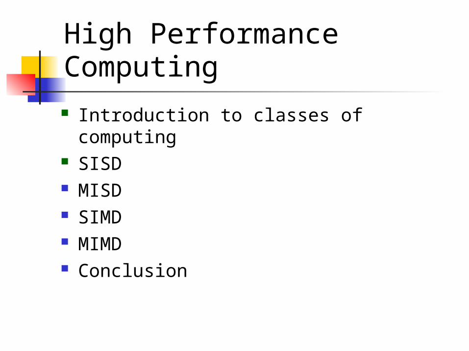
High Performance Computing

Introduction to classes of computing

SISD MISD SIMD MIMD Conclusion

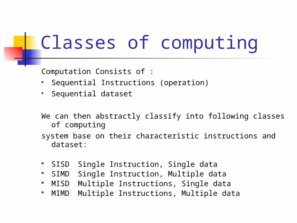
Classes of computingComputation Consists of : Sequential Instructions (operation) Sequential dataset

We can then abstractly classify into following classes of computing

system base on their characteristic instructions and dataset:

SISD Single Instruction, Single data SIMD Single Instruction, Multiple data MISD Multiple Instructions, Single data MIMD Multiple Instructions, Multiple data

High Performance Computing Introduction to classes of computing SISD MISD SIMD MIMD Conclusion

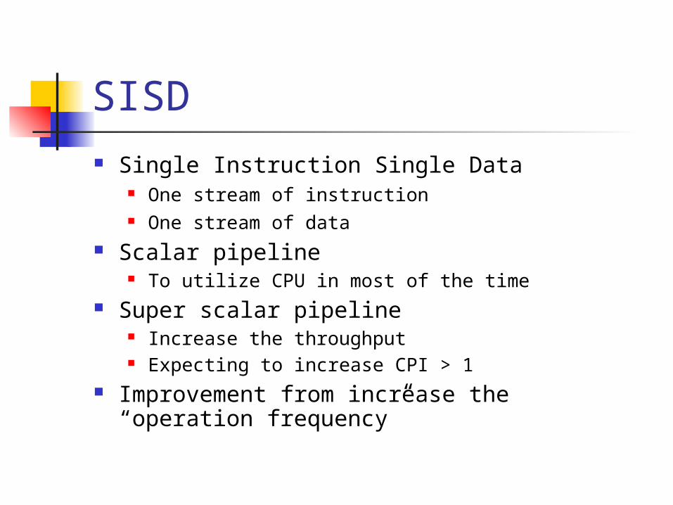
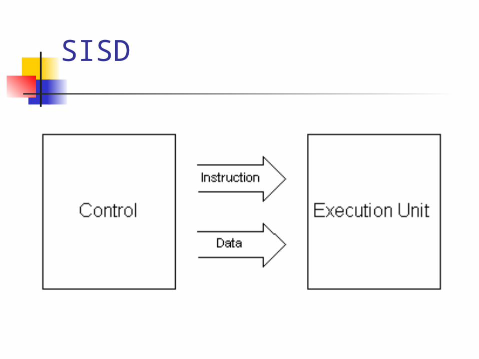
SISD Single Instruction Single Data

One stream of instruction One stream of data

Scalar pipeline To utilize CPU in most of the time

Super scalar pipeline Increase the throughput Expecting to increase CPI > 1

Improvement from increase the “operation frequency”

SISD

SISD

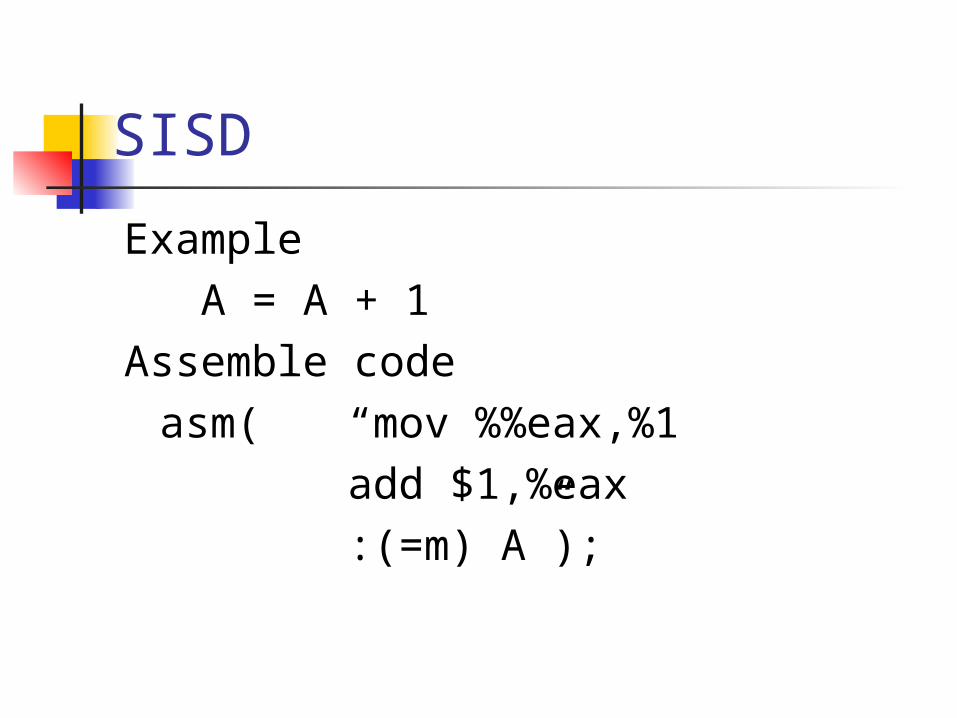
Example A = A + 1Assemble code

asm( “mov %%eax,%1 add $1,%eax

:(=m) A”);

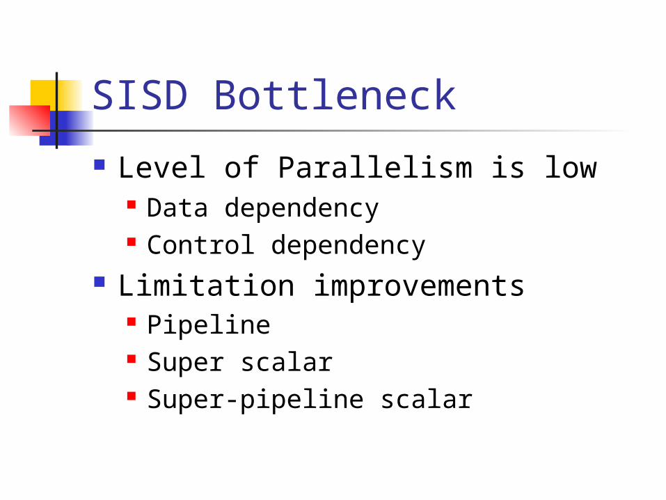
SISD Bottleneck

Level of Parallelism is low Data dependency Control dependency

Limitation improvements Pipeline Super scalar Super-pipeline scalar

High Performance Computing Introduction to classes of computing SISD MISD SIMD MIMD Conclusion

MISD

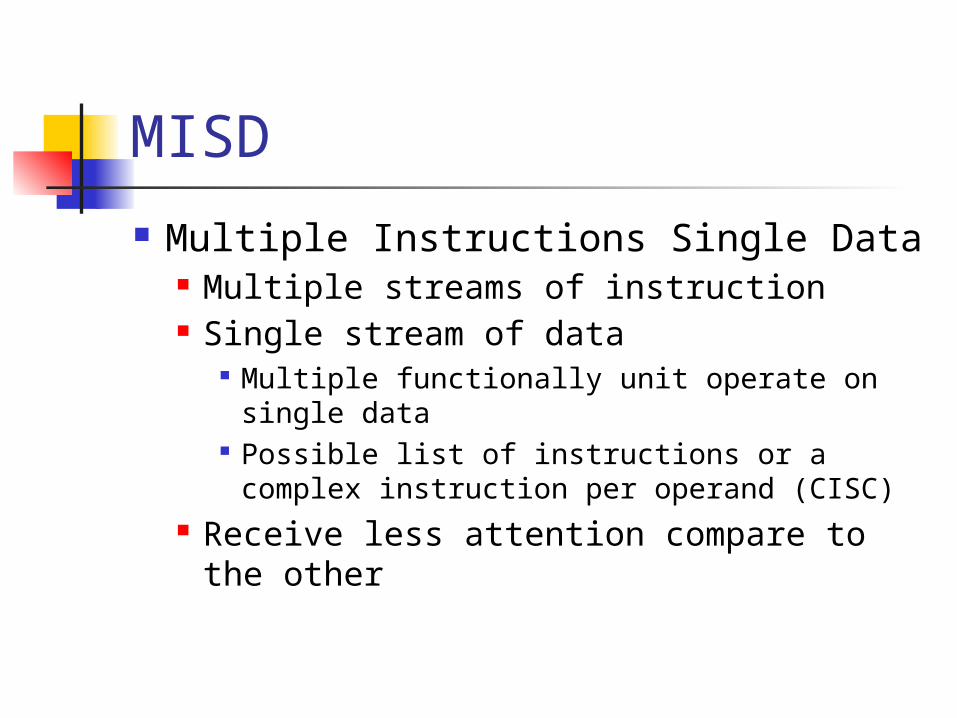
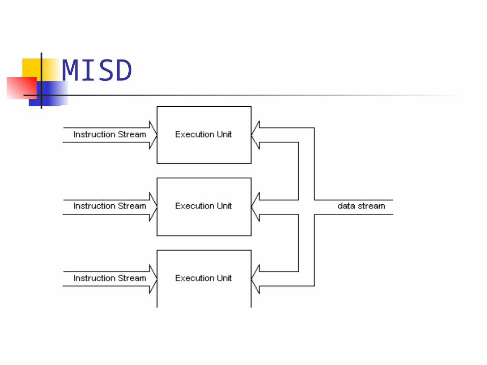
Multiple Instructions Single Data Multiple streams of instruction Single stream of data

Multiple functionally unit operate on single data

Possible list of instructions or a complex instruction per operand (CISC)

Receive less attention compare to the other

MISD

MISD Stream #1

Load R0,%1Add $1,R0Store R1,%1

Stream #2Load R0,%1MUL %1,R0Store R1,%1

MISD

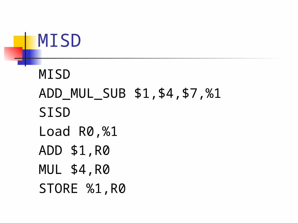
MISDADD_MUL_SUB $1,$4,$7,%1SISDLoad R0,%1ADD $1,R0MUL $4,R0STORE %1,R0

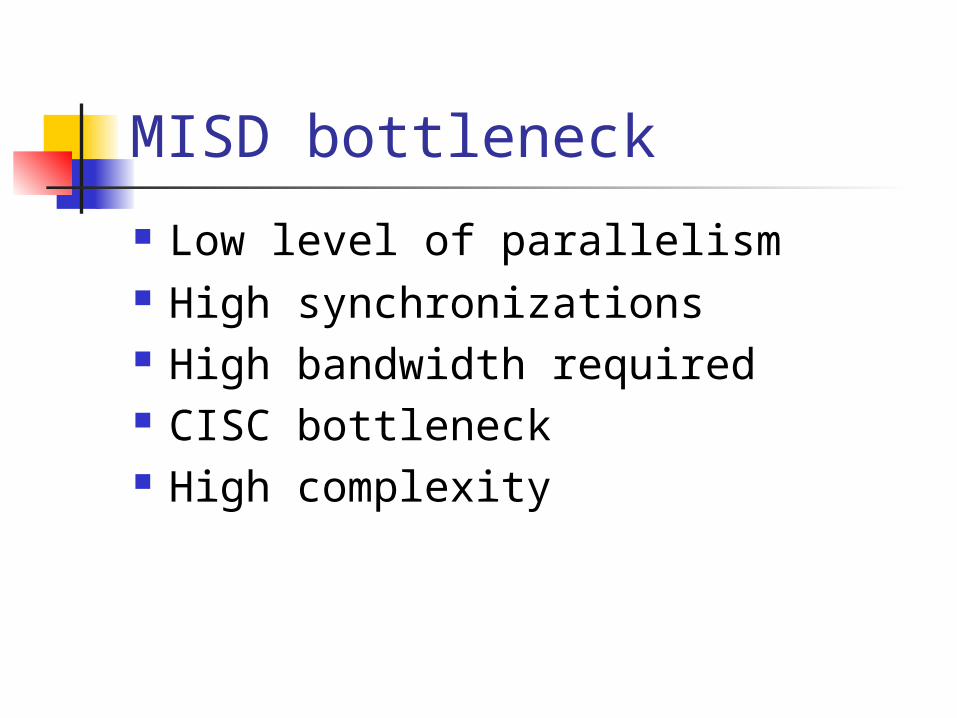
MISD bottleneck

Low level of parallelism High synchronizations High bandwidth required CISC bottleneck High complexity

High Performance Computing Introduction to classes of computing SISD MISD SIMD MIMD Conclusion

SIMD

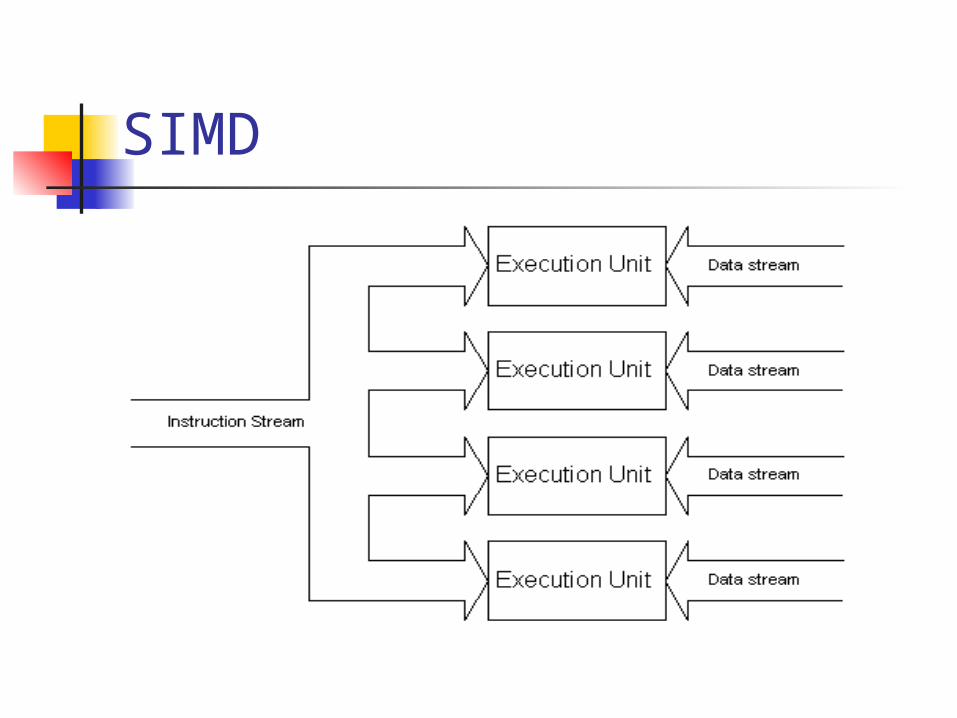
Single Instruction, Multiple Data Single Instruction stream Multiple data streams

Each instruction operate on multiple data in parallel

Fine grained Level of Parallelism

SIMD

SIMD

A wide variety of applications can be solved by parallel algorithms with SIMD only problems that can be divided into

sub problems, all of those can be solved simultaneously by the same set of instructions

This algorithms are typical easy to implement

SIMD Example of

Ordinarily desktop and business applications

Word processor, database , OS and many more

Multimedia applications 2D and 3D image processing, Game and etc

Scientific applications CAD, Simulations

Example of CPU with SIMD ext

Intel P4 & AMD Althon, x86 CPU 8 x 128 bits SIMD registers

G5 Vector CPU with SIMD extension 32 x 128 bits registers

Playstation II 2 vector units with SIMD extension

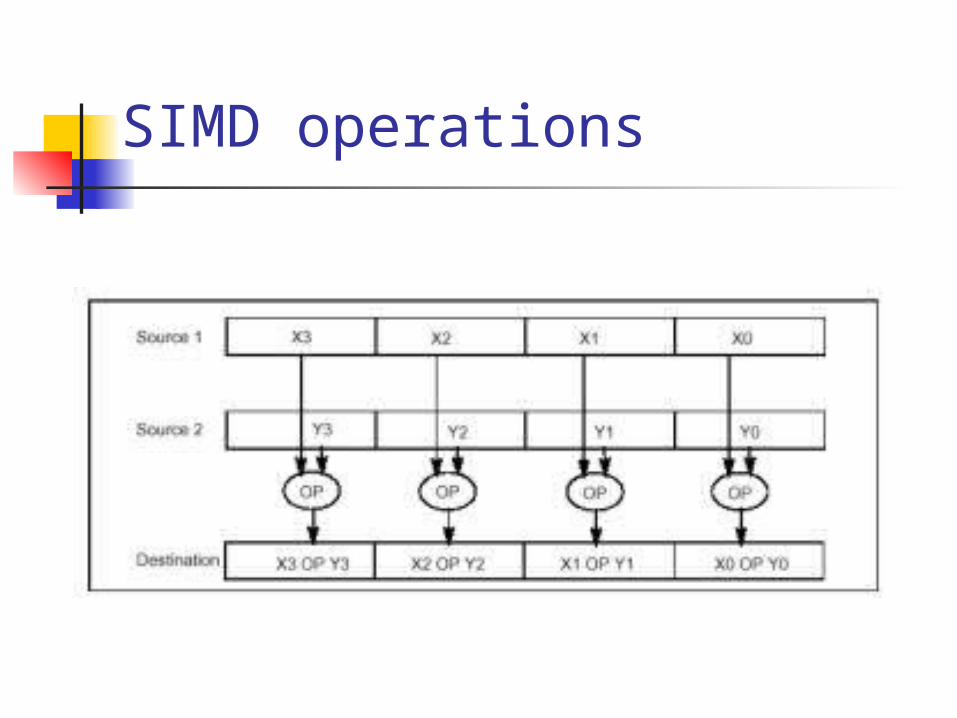
SIMD operations

SIMD

SIMD instructions supports Load and store Integer Floating point Logical and Arithmetic instructions Additional instruction (optional)

Cache instructions to support different locality for different type of application characteristic

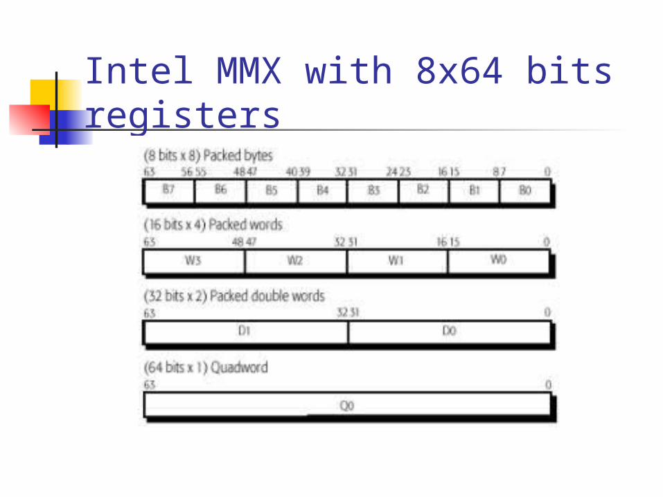
Intel MMX with 8x64 bits registers

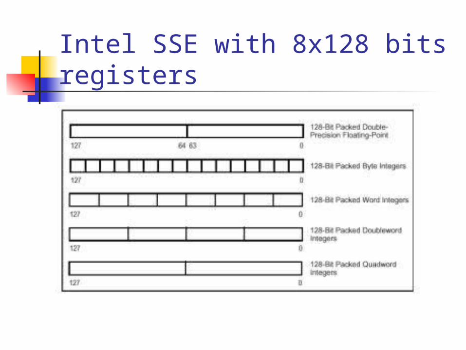
Intel SSE with 8x128 bits registers

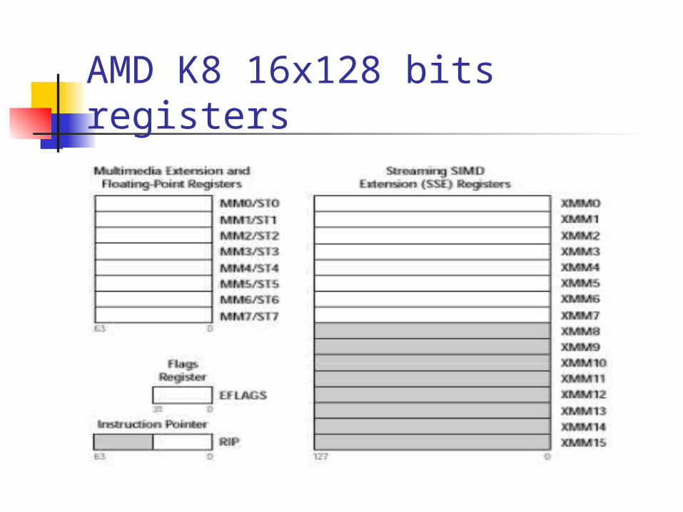
AMD K8 16x128 bits registers

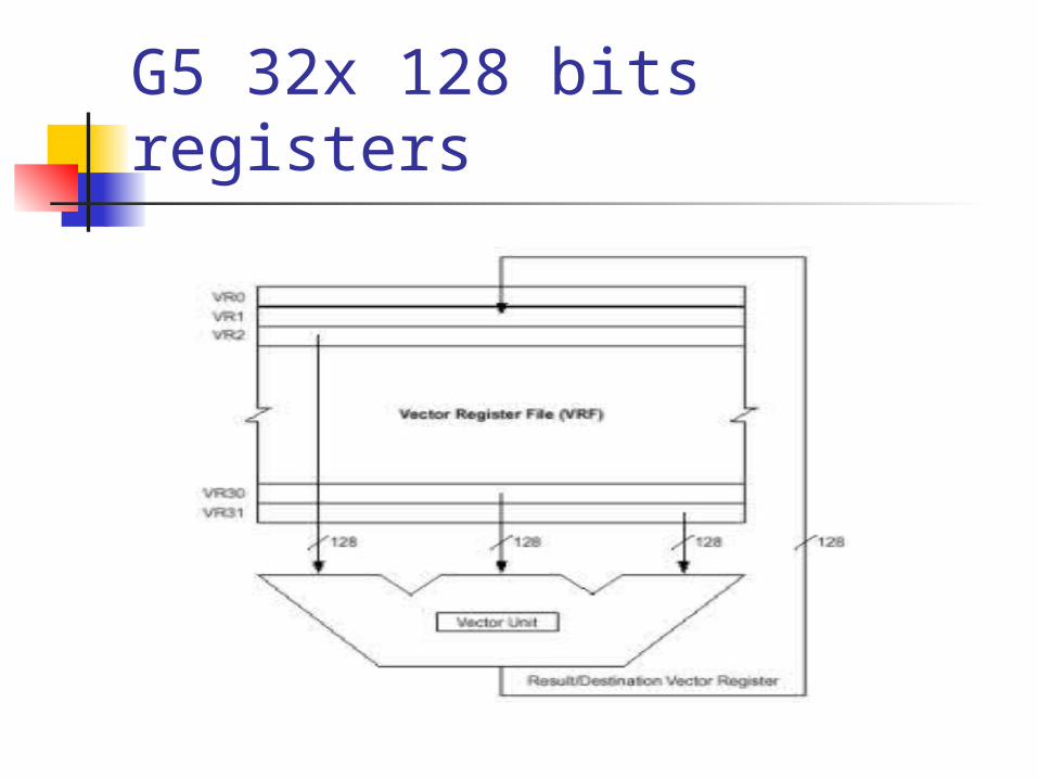
G5 32x 128 bits registers

SIMD

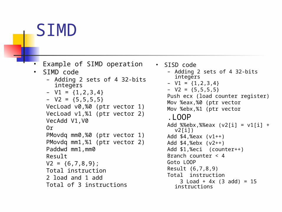
• Example of SIMD operation• SIMD code

– Adding 2 sets of 4 32-bits integers– V1 = {1,2,3,4}– V2 = {5,5,5,5}VecLoad v0,%0 (ptr vector 1)VecLoad v1,%1 (ptr vector 2)VecAdd V1,V0 Or PMovdq mm0,%0 (ptr vector 1)PMovdq mm1,%1 (ptr vector 2)Paddwd mm1,mm0ResultV2 = {6,7,8,9};Total instruction 2 load and 1 add Total of 3 instructions

• SISD code– Adding 2 sets of 4 32-bits integers– V1 = {1,2,3,4}– V2 = {5,5,5,5}Push ecx (load counter register)Mov %eax,%0 (ptr vector Mov %ebx,%1 (ptr vector

.LOOPAdd %%ebx,%%eax (v2[i] = v1[i] + v2[i])Add $4,%eax (v1++)Add $4,%ebx (v2++)Add $1,%eci (counter++)Branch counter < 4Goto LOOPResult {6,7,8,9)Total instruction 3 Load + 4x (3 add) = 15 instructions

SIMD Matrix multiplication

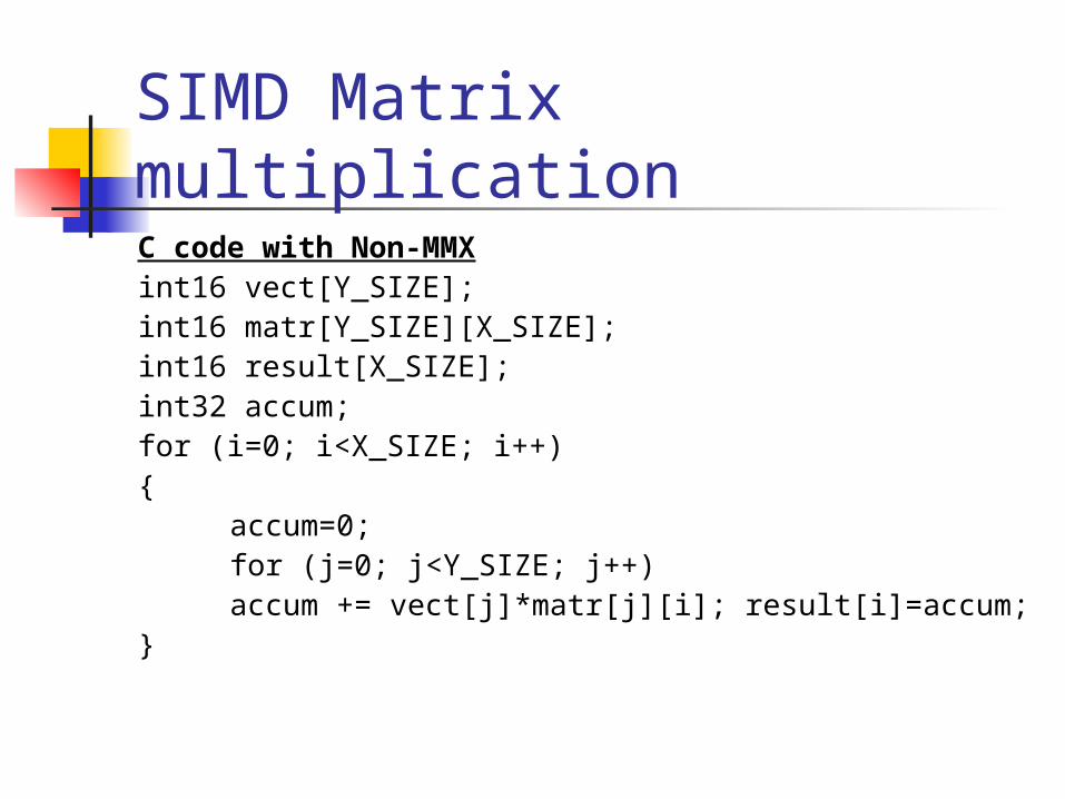
C code with Non-MMXint16 vect[Y_SIZE]; int16 matr[Y_SIZE][X_SIZE]; int16 result[X_SIZE]; int32 accum; for (i=0; i<X_SIZE; i++) {

accum=0; for (j=0; j<Y_SIZE; j++) accum += vect[j]*matr[j][i]; result[i]=accum;

}

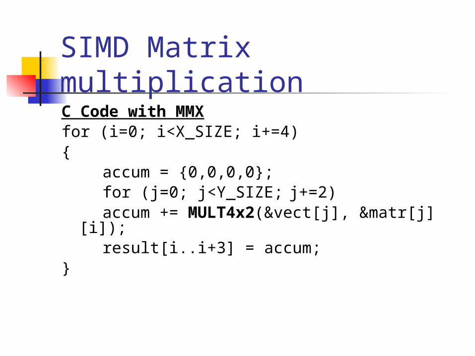
SIMD Matrix multiplicationC Code with MMXfor (i=0; i<X_SIZE; i+=4) {

accum = {0,0,0,0}; for (j=0; j<Y_SIZE; j+=2) accum += MULT4x2(&vect[j], &matr[j][i]);

result[i..i+3] = accum; }

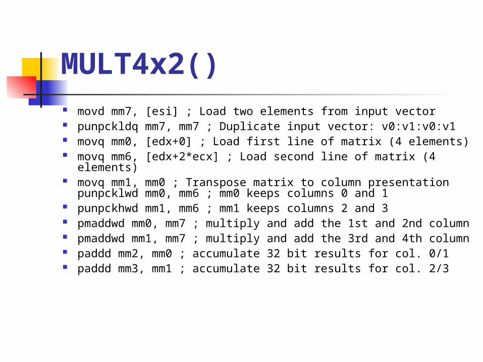
MULT4x2() movd mm7, [esi] ; Load two elements from input vector punpckldq mm7, mm7 ; Duplicate input vector: v0:v1:v0:v1 movq mm0, [edx+0] ; Load first line of matrix (4 elements) movq mm6, [edx+2*ecx] ; Load second line of matrix (4

elements) movq mm1, mm0 ; Transpose matrix to column presentation

punpcklwd mm0, mm6 ; mm0 keeps columns 0 and 1 punpckhwd mm1, mm6 ; mm1 keeps columns 2 and 3 pmaddwd mm0, mm7 ; multiply and add the 1st and 2nd

column pmaddwd mm1, mm7 ; multiply and add the 3rd and 4th

column paddd mm2, mm0 ; accumulate 32 bit results for col. 0/1 paddd mm3, mm1 ; accumulate 32 bit results for col. 2/3

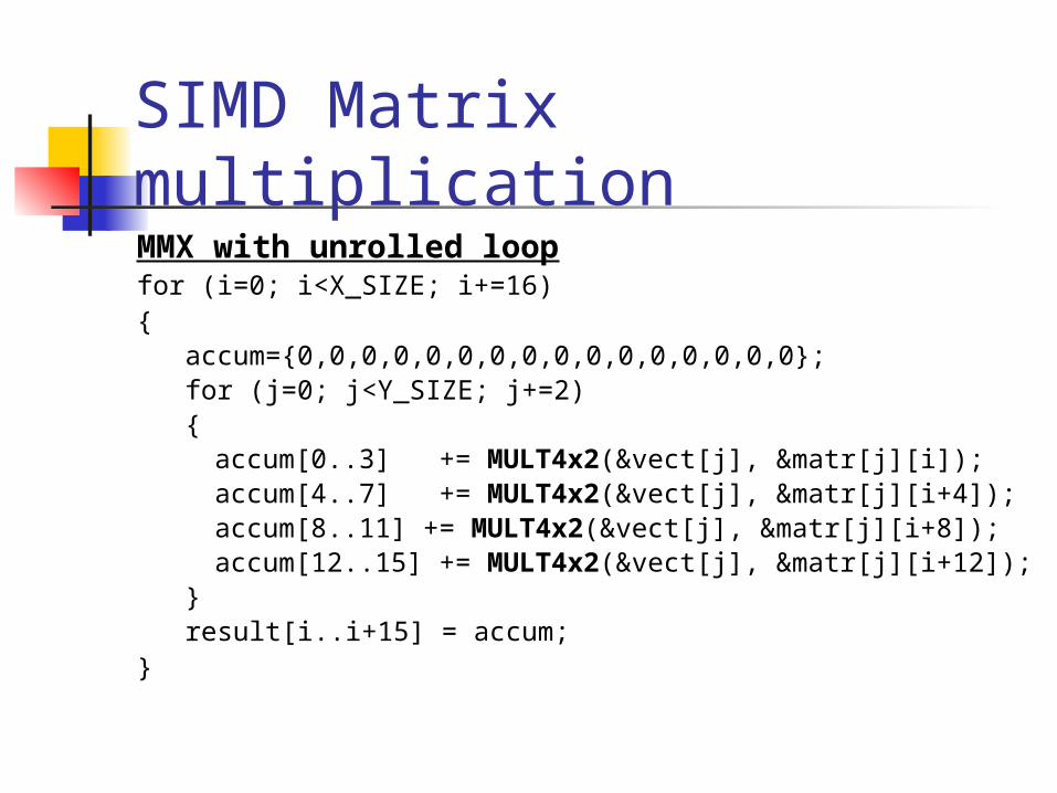
SIMD Matrix multiplicationMMX with unrolled loopfor (i=0; i<X_SIZE; i+=16) {

accum={0,0,0,0,0,0,0,0,0,0,0,0,0,0,0,0};for (j=0; j<Y_SIZE; j+=2) {

accum[0..3] += MULT4x2(&vect[j], &matr[j][i]); accum[4..7] += MULT4x2(&vect[j], &matr[j][i+4]); accum[8..11] += MULT4x2(&vect[j], &matr[j][i+8]); accum[12..15] += MULT4x2(&vect[j], &matr[j][i+12]);

} result[i..i+15] = accum;

}

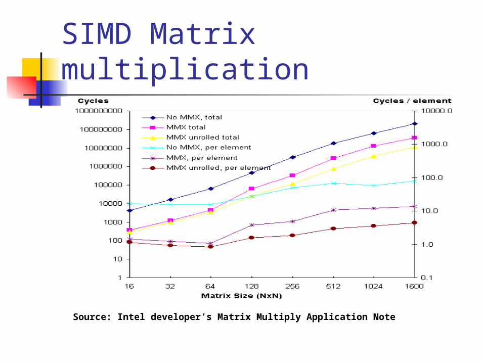
SIMD Matrix multiplication

Source: Intel developer’s Matrix Multiply Application Note

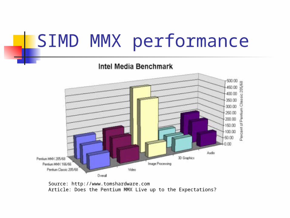
SIMD MMX performance

Source: http://www.tomshardware.comArticle: Does the Pentium MMX Live up to the Expectations?

High Performance Computing

Introduction to classes of computing

SISD MISD SIMD MIMD Conclusion

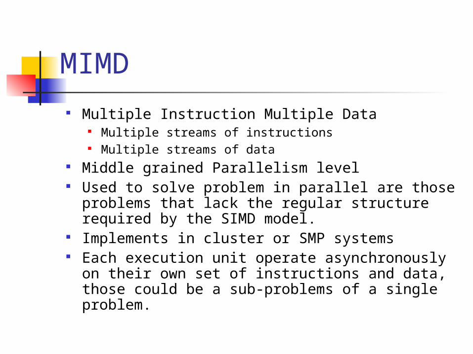
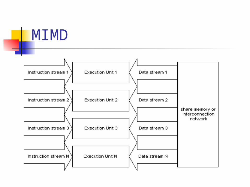
MIMD

Multiple Instruction Multiple Data Multiple streams of instructions Multiple streams of data

Middle grained Parallelism level Used to solve problem in parallel are those

problems that lack the regular structure required by the SIMD model.

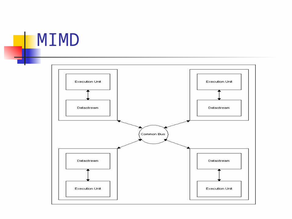
Implements in cluster or SMP systems Each execution unit operate asynchronously

on their own set of instructions and data, those could be a sub-problems of a single problem.

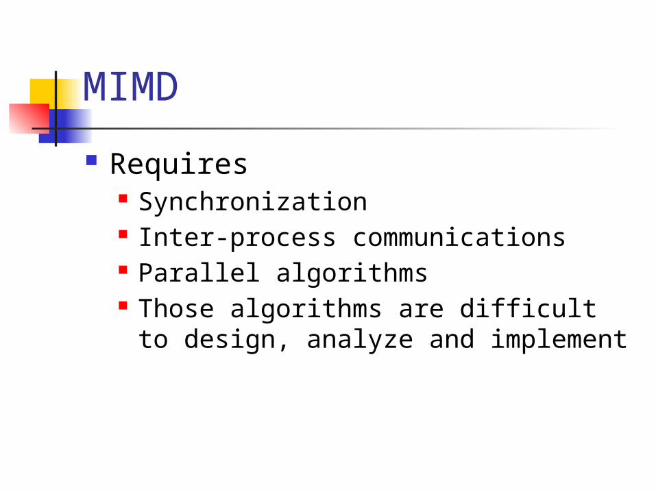
MIMD

Requires Synchronization Inter-process communications Parallel algorithms Those algorithms are difficult to

design, analyze and implement

MIMD

MIMD

MPP Super-computer

High performance of single processor

Multi-processor MP Cluster Network Mixture of everything

Cluster of High performance MP nodes

Example of MPP Machines

Earth Simulator (2002) Cray C90 Cray X-MP

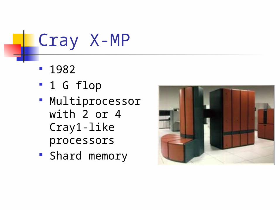
Cray X-MP 1982 1 G flop Multiprocessor

with 2 or 4 Cray1-like processors

Shard memory

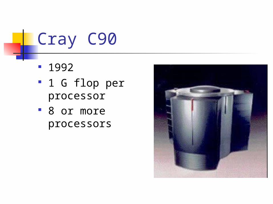
Cray C90 1992 1 G flop per

processor 8 or more

processors

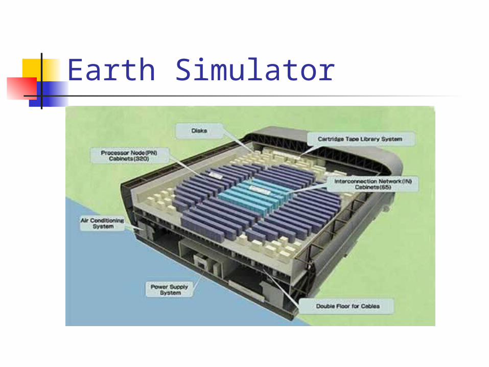
The Earth Simulator

Operational in late 2002 Result of 5-year design and

implementation effort Equivalent power to top 15 US

Machines

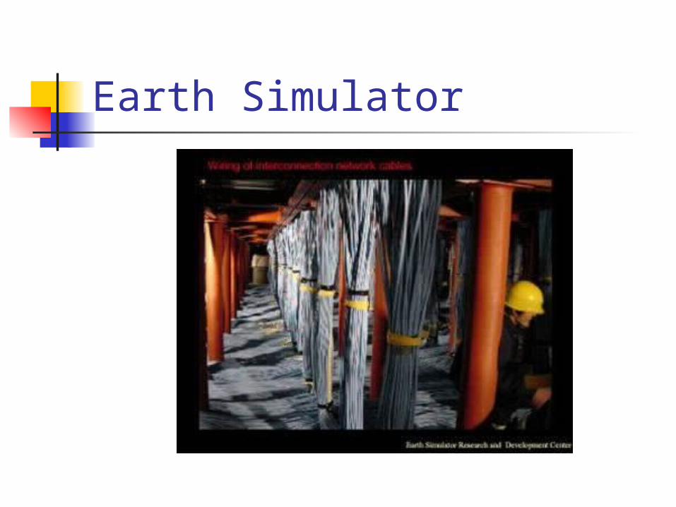
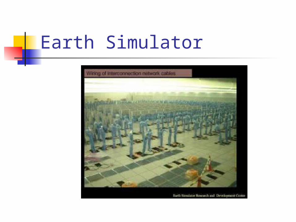
The Earth Simulator in details 640 nodes 8 vector processors per node, 5120 total 8 G flops per processor, 40 T flops total 16 GB memory per node, 10 TB total 2800 km of cables 320 cabinets (2 nodes each) Cost: $ 350 million

Earth Simulator

Earth Simulator

Earth Simulator

Earth Simulator

Earth Simulator

High Performance Computing

Introduction to classes of computing

SISD MISD SIMD MIMD Conclusion

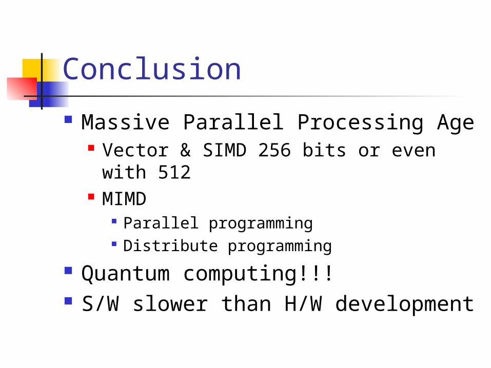
Conclusion

Massive Parallel Processing Age Vector & SIMD 256 bits or even with

512 MIMD

Parallel programming Distribute programming

Quantum computing!!! S/W slower than H/W development

Appendix Very High-Speed Computing System

Michael J. Flynn, member, IEEE

Into the Fray With SIMD www.cs.umd.edu/class/fall2001/cmsc411/projects/SIMDproj/project.htm

Understanding SIMD http://developer.apple.com

Matrix Multiply Application Note www.intel.com

Parallel Computing Systems Dror Feitelson, Hebrew University

Does the Pentium MMX Live up to the Expectations? www.tomshardware.com

End of Talk

^_^

Thank you

High Performance Computing