high fidelity system simulation of multiple components … · high fidelity system simulation of...
TRANSCRIPT

Ronald C. Plybon and Allan VanDeWall
GE Aircraft Engines, Cincinnati, Ohio
Rajiv Sampath, Mahadevan Balasubramaniam, Ramakrishna Mallina,
and Rohinton Irani
GE Global Research Center, Niskayuna, New York
High Fidelity System Simulation of MultipleComponents in Support of the UEET Program
NASA/CR—2006-214230
April 2006
https://ntrs.nasa.gov/search.jsp?R=20060012153 2018-07-07T18:17:33+00:00Z

NASA STI Program . . . in Profile
Since its founding, NASA has been dedicated to the
advancement of aeronautics and space science. The
NASA Scientific and Technical Information (STI)
program plays a key part in helping NASA maintain
this important role.
The NASA STI Program operates under the auspices
of the Agency Chief Information Officer. It collects,
organizes, provides for archiving, and disseminates
NASA’s STI. The NASA STI program provides access
to the NASA Aeronautics and Space Database and its
public interface, the NASA Technical Reports Server,
thus providing one of the largest collections of
aeronautical and space science STI in the world.
Results are published in both non-NASA channels and
by NASA in the NASA STI Report Series, which
includes the following report types:
• TECHNICAL PUBLICATION. Reports of
completed research or a major significant phase
of research that present the results of NASA
programs and include extensive data or theoretical
analysis. Includes compilations of significant
scientific and technical data and information
deemed to be of continuing reference value.
NASA counterpart of peer-reviewed formal
professional papers but has less stringent
limitations on manuscript length and extent of
graphic presentations.
• TECHNICAL MEMORANDUM. Scientific
and technical findings that are preliminary or
of specialized interest, e.g., quick release
reports, working papers, and bibliographies that
contain minimal annotation. Does not contain
extensive analysis.
• CONTRACTOR REPORT. Scientific and
technical findings by NASA-sponsored
contractors and grantees.
• CONFERENCE PUBLICATION. Collected
papers from scientific and technical
conferences, symposia, seminars, or other
meetings sponsored or cosponsored by NASA.
• SPECIAL PUBLICATION. Scientific,
technical, or historical information from
NASA programs, projects, and missions, often
concerned with subjects having substantial
public interest.
• TECHNICAL TRANSLATION. English-
language translations of foreign scientific and
technical material pertinent to NASA’s mission.
Specialized services also include creating custom
thesauri, building customized databases, organizing
and publishing research results.
For more information about the NASA STI
program, see the following:
• Access the NASA STI program home page at
http://www.sti.nasa.gov
• E-mail your question via the Internet to
• Fax your question to the NASA STI Help Desk
at 301–621–0134
• Telephone the NASA STI Help Desk at
301–621–0390
• Write to:
NASA STI Help Desk
NASA Center for AeroSpace Information
7121 Standard Drive
Hanover, MD 21076–1320

High Fidelity System Simulation of MultipleComponents in Support of the UEET Program
NASA/CR—2006-214230
April 2006
National Aeronautics and
Space Administration
Glenn Research Center
Cleveland, Ohio 44135
Prepared under Contract NAS3–01135, Task Order #6
Ronald C. Plybon and Allan VanDeWall
GE Aircraft Engines, Cincinnati, Ohio
Rajiv Sampath, Mahadevan Balasubramaniam, Ramakrishna Mallina,
and Rohinton Irani
GE Global Research Center, Niskayuna, New York

Acknowledgments
The authors would also like to acknowledge the following engineers at GE Aircraft Engines for their help and consultation
during several phases of this contract: Randy Cepress, Rick Berg, Scott Carson, Andrew Breeze-Stringfellow, Katherine Treml,
Noel Macsotai, and Tom Moniz. Finally, the team would like to acknowledge the support and technical contributions of the
following NASA personnel who contributed to this effort: JohnAdamczyk, Clayton Meyers, Russell Claus, Scott Jones, Louis
Larosiliere, Joseph Veres, Gregory Follen, and Thomas Lavelle.
Available from
NASA Center for Aerospace Information
7121 Standard Drive
Hanover, MD 21076–1320
National Technical Information Service
5285 Port Royal Road
Springfield, VA 22161
Available electronically at http://gltrs.grc.nasa.gov
Trade names and trademarks are used in this report for identification
only. Their usage does not constitute an official endorsement,
either expressed or implied, by the National Aeronautics and
Space Administration.
This work was sponsored by the Fundamental Aeronautics Program
at the NASA Glenn Research Center.
Level of Review: This material has been technically reviewed by NASA technical management.

NASA/CR—2006-214230 iii
Contents 1.0 Executive Summary ...................................................................................................... 1 1.1 Project Scope and Key Deliverables .................................................................... 1 1.2 Uncertainty Metrics............................................................................................... 3 1.3 Technology Roadmap .......................................................................................... 5 1.4 Program Accomplishments .................................................................................. 5
2.0 HLTM Intermediate Fidelity System Simulation ............................................................ 7 2.1 Aerodynamic Zooming using Blade Row Model................................................... 7 2.2 Cooling Flow Studies............................................................................................ 10 2.3 Geometry Zooming using Morphing Techniques ................................................. 11 2.4 Compressor Mechanical Analysis ........................................................................ 14 2.5 500 nm Mission Fuel-Burn Roll-UP ...................................................................... 14
3.0 HLTM High Fidelity System Simulation......................................................................... 16 3.1 High Fidelity CFD Feedback to NPSS.................................................................. 16 3.2 Improved Component Simulations via Multi-Stage Unsteady CFD...................... 17
4.0 Uncertainty Metric Roll-Up ............................................................................................ 27 4.1 Uncertainty Reduction via High-Fidelity System Simulation at TG 3.................... 27
5.0 Conclusions .................................................................................................................. 33
6.0 References………. ........................................................................................................ 33


NASA/CR—2006-214230 1
High Fidelity System Simulation of Multiple Components in Support of the UEET Program
Ronald C. Plybon and Allan VanDeWall
GE Aircraft Engines Cincinnati, Ohio 45215
Rajiv Sampath, Mahadevan Balasubramaniam, Ramakrishna Mallina, and Rohinton Irani
GE Global Research Center Niskayuna, New York 12309
1.0 Executive Summary 1.1 Project Scope and Key Deliverables
Introduction The design process for turbomachinery components contains several levels of fidelity,
progressing from the 0-D cycle analysis to 2-D axisymmetric flow analysis followed by full 3-D geometry definition and analysis. During each step of the analysis process, the Numerical Propulsion System Simulation (NPSS), (ref. 1), concept of zooming between analysis fidelity levels is applied for consistency and accuracy. A second aspect of the design process is the exchange of geometry and flow parameters between components, for example between a combustor and turbine. A third aspect of the design process is the flow of geometry and analysis data between disciplines for a single component, for instance the aerodynamic, heat transfer and stress analysis in the optimization of a turbine blade.
To effectively address these three design system requirements, the necessary framework must be in place to provide the system level environment, specific analysis tools and high performance computing resources. At the highest level of fidelity, 3-D Navier-Stokes flow simulations are a key part of the design system. In reviewing the progression of 3-D Navier-Stokes simulations for turbomachinery, a building block or stepwise approach has been taken to reach the current state-of-the-art. Starting with inviscid simulations in the 1980’s, designers are now able to apply steady and unsteady, viscous codes to combustors and multistage bladerows on a regular basis. These advancements have led to significant improvements in turbomachinery prediction accuracy and design productivity. The eventual goal of NPSS is to enable a system that is capable of analyzing the operation of a propulsion system in sufficient detail to resolve the effects of multidisciplinary processes and component interactions, currently only observable in large-scale tests. The vision is to create a “numerical test cell” that enables engineers to examine various design options without having to conduct costly and time-consuming real-life tests. Towards this end, NASA’s NPSS team is working closely with academia and industry partners such as GE Aircraft Engines to develop a full-engine simulation system (see fig. 1) capable of: (a) Integration between different components (b) Coupling between different analysis disciplines (c) Zooming between model fidelities.
Traditionally, the design of a jet engine begins with a study of the complete engine using a relatively simple aero-thermodynamic “cycle” analysis. The characteristics of the various engine components such as fan, compressor, turbine, etc. are represented in the study by performance maps, which are based on higher-fidelity analysis and experimental test data. As the process moves forward, the design of the individual engine components is further refined, simulated and experimentally tested in isolation by component design teams. These results are then used to

NASA/CR—2006-214230 2
Figure 1.—NPSS simulation cube.
calibrate the component performance maps and improve the cycle analysis of the complete engine. This iterative process continues, with component designs being refined, until both component and engine performance goals are fully met. Component design teams rely on advanced numerical techniques to understand component operation and achieve the best performance. Streamline curvature methods (ref. 2), which calculate flow properties at multiple streamlines across the component’s span, continue to be widely used in turbomachinery design and analysis. More recently, advances in computing technology have enabled advanced two- and three-dimensional numerical techniques to be applied to the design of isolated components. Methods for simulating multistage turbomachinery have also been developed by researchers, and are now being regularly applied in the design process (refs. 3 and 4).
While advanced numerical simulations of isolated components may yield detailed performance data at unique component operating points, they do not systematically account for interactions between engine components. Overall engine performance is dependent on the components working together efficiently over a range of demanding operating conditions with components that are sensitive to interactions with adjoining components. For example, compressor performance is very sensitive to steady inlet and outlet flow conditions, and abrupt flow changes in the compressor can unstart a supersonic inlet. Consequently, it is important to consider the engine as a system of components that influence each other, and not simply isolated components. Although performance maps attempt to capture component interactions, a high-fidelity full-engine simulation can provide more details about component interactions. Towards this vision, the present work was undertaken to extend engine simulation capability in NPSS from isolated components to the full engine, by integrating advanced intermediate- and high-fidelity component simulation codes to allow a designer to obtain detailed three-dimensional representation of the engine at multiple operating points early in the design. In the following discussion, the authors present results that demonstrate how these elements of NPSS have been used effectively by a joint GE/NASA team on the contract to develop aerodynamic, mechanical and aero-mechanical high-fidelity analysis capabilities within NPSS that could eventually pave the way towards an automated three-dimensional simulation of a complete turbofan engine.
NASA/CR—2006-214230 3
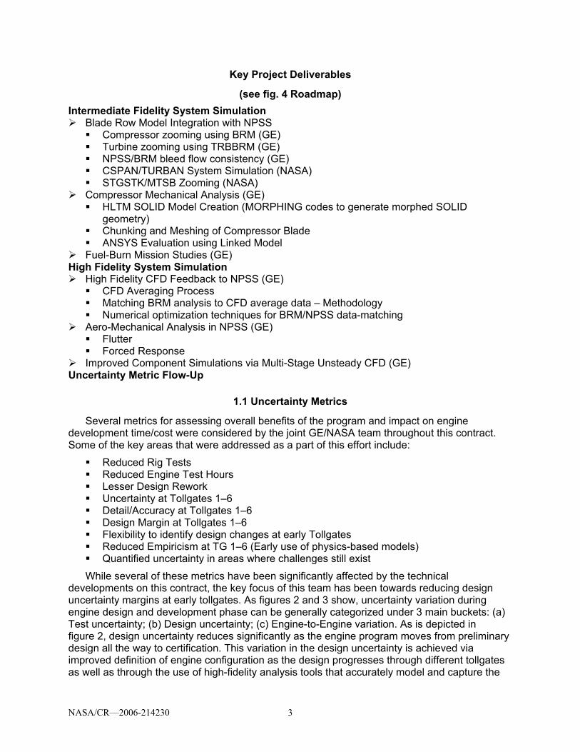
Key Project Deliverables
(see fig. 4 Roadmap) Intermediate Fidelity System Simulation
Blade Row Model Integration with NPSS Compressor zooming using BRM (GE) Turbine zooming using TRBBRM (GE) NPSS/BRM bleed flow consistency (GE) CSPAN/TURBAN System Simulation (NASA) STGSTK/MTSB Zooming (NASA)
Compressor Mechanical Analysis (GE) HLTM SOLID Model Creation (MORPHING codes to generate morphed SOLID
geometry) Chunking and Meshing of Compressor Blade ANSYS Evaluation using Linked Model
Fuel-Burn Mission Studies (GE) High Fidelity System Simulation
High Fidelity CFD Feedback to NPSS (GE) CFD Averaging Process Matching BRM analysis to CFD average data – Methodology Numerical optimization techniques for BRM/NPSS data-matching
Aero-Mechanical Analysis in NPSS (GE) Flutter Forced Response
Improved Component Simulations via Multi-Stage Unsteady CFD (GE) Uncertainty Metric Flow-Up
1.1 Uncertainty Metrics
Several metrics for assessing overall benefits of the program and impact on engine development time/cost were considered by the joint GE/NASA team throughout this contract. Some of the key areas that were addressed as a part of this effort include:
Reduced Rig Tests Reduced Engine Test Hours Lesser Design Rework Uncertainty at Tollgates 1–6 Detail/Accuracy at Tollgates 1–6 Design Margin at Tollgates 1–6 Flexibility to identify design changes at early Tollgates Reduced Empiricism at TG 1–6 (Early use of physics-based models) Quantified uncertainty in areas where challenges still exist
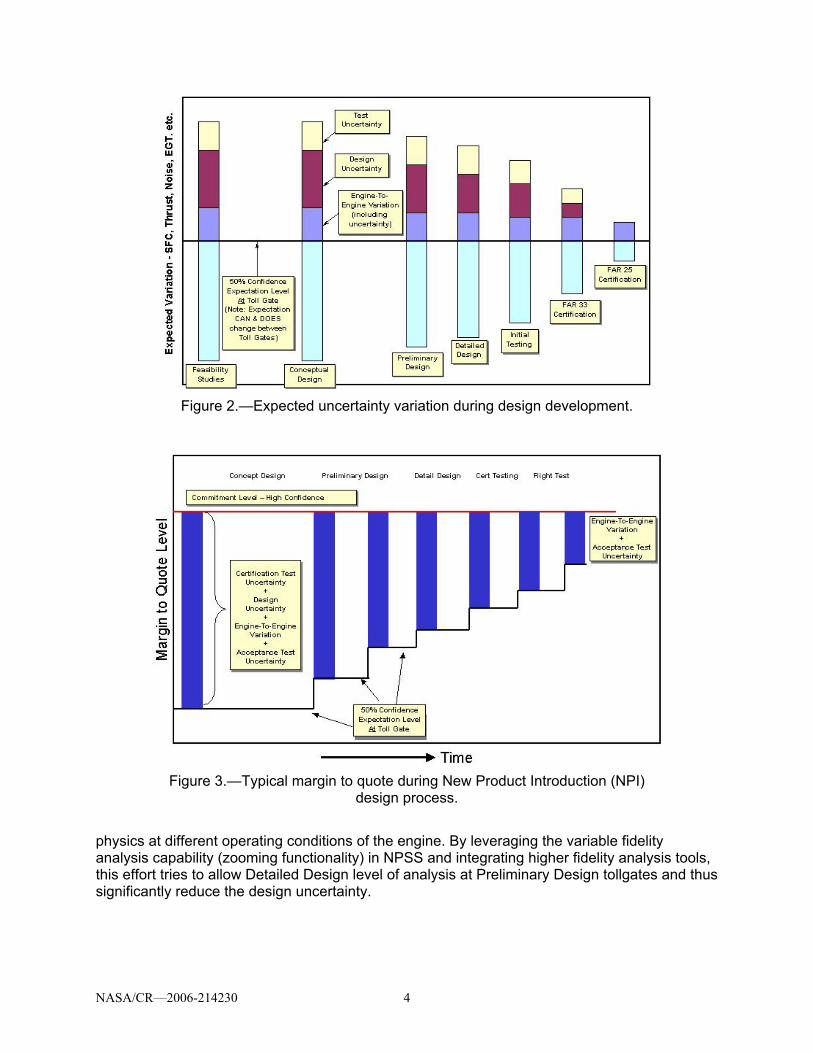
While several of these metrics have been significantly affected by the technical developments on this contract, the key focus of this team has been towards reducing design uncertainty margins at early tollgates. As figures 2 and 3 show, uncertainty variation during engine design and development phase can be generally categorized under 3 main buckets: (a) Test uncertainty; (b) Design uncertainty; (c) Engine-to-Engine variation. As is depicted in figure 2, design uncertainty reduces significantly as the engine program moves from preliminary design all the way to certification. This variation in the design uncertainty is achieved via improved definition of engine configuration as the design progresses through different tollgates as well as through the use of high-fidelity analysis tools that accurately model and capture the
NASA/CR—2006-214230 4
Figure 2.—Expected uncertainty variation during design development.
Figure 3.—Typical margin to quote during New Product Introduction (NPI)
design process.
physics at different operating conditions of the engine. By leveraging the variable fidelity analysis capability (zooming functionality) in NPSS and integrating higher fidelity analysis tools, this effort tries to allow Detailed Design level of analysis at Preliminary Design tollgates and thus significantly reduce the design uncertainty.
NASA/CR—2006-214230 5
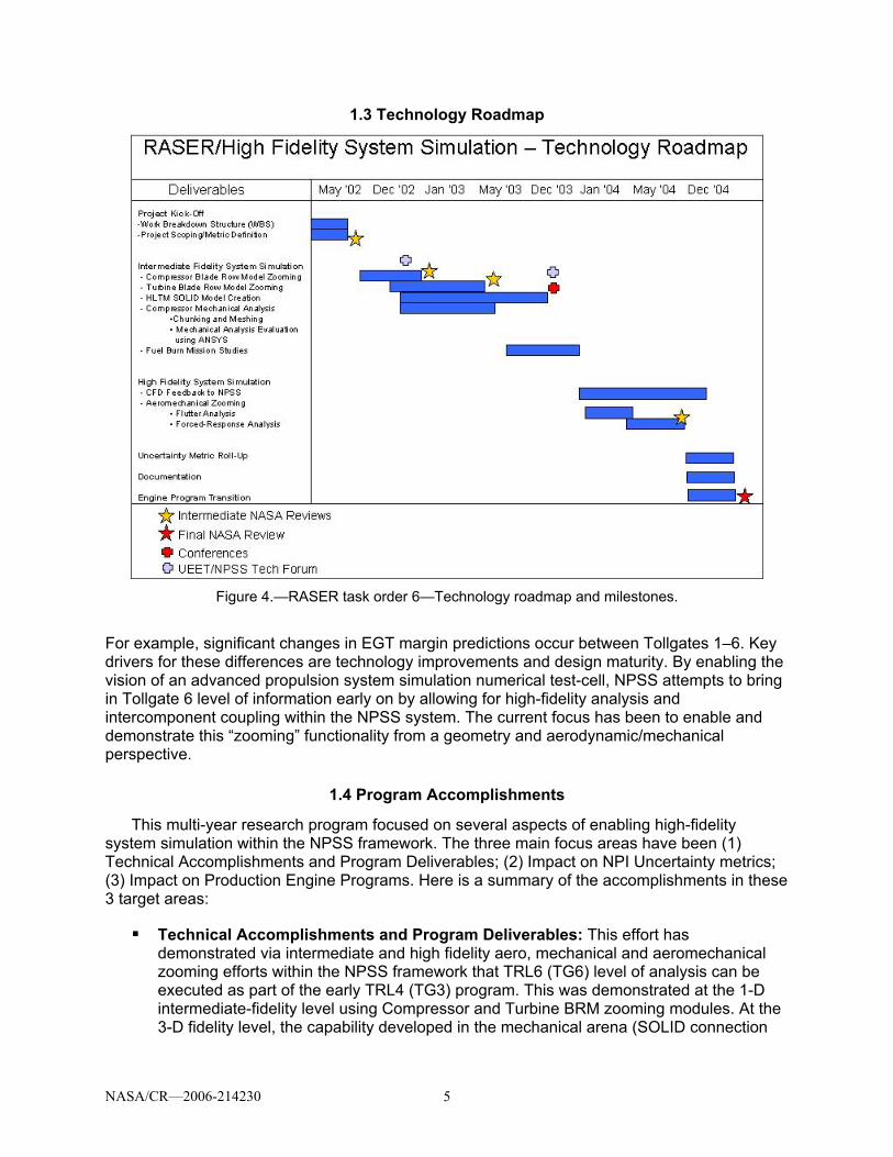
1.3 Technology Roadmap
Figure 4.—RASER task order 6—Technology roadmap and milestones.
For example, significant changes in EGT margin predictions occur between Tollgates 1–6. Key drivers for these differences are technology improvements and design maturity. By enabling the vision of an advanced propulsion system simulation numerical test-cell, NPSS attempts to bring in Tollgate 6 level of information early on by allowing for high-fidelity analysis and intercomponent coupling within the NPSS system. The current focus has been to enable and demonstrate this “zooming” functionality from a geometry and aerodynamic/mechanical perspective.
1.4 Program Accomplishments
This multi-year research program focused on several aspects of enabling high-fidelity system simulation within the NPSS framework. The three main focus areas have been (1) Technical Accomplishments and Program Deliverables; (2) Impact on NPI Uncertainty metrics; (3) Impact on Production Engine Programs. Here is a summary of the accomplishments in these 3 target areas:
Technical Accomplishments and Program Deliverables: This effort has
demonstrated via intermediate and high fidelity aero, mechanical and aeromechanical zooming efforts within the NPSS framework that TRL6 (TG6) level of analysis can be executed as part of the early TRL4 (TG3) program. This was demonstrated at the 1-D intermediate-fidelity level using Compressor and Turbine BRM zooming modules. At the 3-D fidelity level, the capability developed in the mechanical arena (SOLID connection

NASA/CR—2006-214230 6
and the corresponding mechanical analysis modules) as well as developments on the aero analysis and feedback side, wherein high-fidelity CFD models was employed to improve the fidelity of intermediate fidelity models such as BRM helped achieve this goal. These studies have shown that there are significant advantages to both the “feed-forward” (i.e., zooming) as well as “feedback” approach of enabling high-fidelity analysis in NPSS. The “feed-forward” approach allows a designer to assess a certain critical operating points and execute detailed high-fidelity analysis at TRL4 that would otherwise not be available at this stage in the design. This information would allow the designer to qualitatively update critical preliminary design parameters to meet program goals based on accurate high-fidelity analysis results. The “feedback” approach of zooming demonstrated in the CFD analysis feedback to NPSS has shown that high-fidelity analysis results can not only be used qualitatively; but also quantitatively, to directly update intermediate fidelity system models and improve the overall predictions of SFC, EGT, Fuel Burn and other important metrics.
Impact on NPI Uncertainty Metrics: As the analysis in chapter 4 describes, several improvements addressed in the course of this contract result in a net improvement in the overall NPI uncertainty margins. The improvements come from additional information as well as improved accuracy via intermediate and high fidelity system simulation capability within NPSS.
Impact on Production Engine Programs: As part of GE Aircraft Engine’s committment to take research developments resulting out of government contract efforts to production mode, wherein there is significant application of these techniques and methodologies on on-going and planned engine programs, additional efforts are currently on-going with support from GE Aircraft Engine’s internal R&D funds to apply these techniques to on-going programs. Significant advancements have already been made towards this goal and the research team is actively working towards this goal along with support from engineers from GE Aircraft Engine’s NPI programs.
NASA/CR—2006-214230 7
2.0 HLTM Intermediate Fidelity System Simulation 2.1 Aerodynamic Zooming Using Blade Row Model
NPSS Models and Component Maps NPSS in its current status represents a sophisticated thermodynamic system modeling
software along with toolkits developed to couple high-fidelity codes such as 3D-CFD and mechanical analysis tools. An NPSS engine cycle model typically uses simple mathematical representations of the aerothermodynamics of the internal flow in the engine. The model is used to determine all pertinent performance data for a given flight condition when the component characteristics and operating conditions are known. NPSS uses a component-based, object-oriented approach to model different engine configurations. An NPSS engine model is assembled from a collection of interconnected elements and sub-elements, and controlled by a numerical solver. Components such as the compressor or turbine are represented by a corresponding element that models the associated thermodynamics. The component map is modeled using an associated sub-element. The model is defined using the NPSS programming language, and can be executed in interpreted or compiled mode by the NPSS software. The numerical solver is used to ensure matching between various components, such as the difference between the predicted flow exiting a component and the flow capacity of a downstream component. Finally, the model uses modifiers to account for secondary effects such as the Reynolds number effects, clearance effects, blade untwist effects, cooling flow effects, etc.
The NPSS cycle model has one map for each major component and is plugged into the NPSS model as a sub-element. The map characterizes the component’s response to the boundary conditions imposed on it by the engine system. The complete component performance predicted by the cycle model is the combination of the map performance and a variety of corrections for secondary effects. The GE Aircraft Engines (GEAE) design process uses a Blade Row Model (BRM) for generating the necessary maps for the various components within the cycle model. BRM is an in-house program that can automatically generate maps in the min-loss stage characteristic or backbone map form used at GEAE. Figures 5 and 6 show example compressor and turbine maps generated using the Blade Row Model program.
The maps shown in figure 5 and 6 have been evaluated at standard operating conditions of pressure, temperature and secondary effects such as bleed flow, variable stator vane position, gas properties, etc. To account for variation of the secondary effects with operating conditions, NPSS models employ several empirical modifiers to correct for the deviation from the standard conditions assumed in the map-generation process. These overall empirical correlation adjustments have an underlying physics-based representation, but still introduce significant uncertainty without real test data for validation. As the discussion below will describe, by bringing in a tight coupling with intermediate fidelity codes such as the BRM, NPSS models can reduce the need for these overall empirical corrections and employ more physics-based models early in the design and hence reduce this simulation uncertainty.

NASA/CR—2006-214230 8
Figure 5.—Example compressor map.
Figure 6.—Example turbine map.
As such, NPSS cycle models use a compressor and turbine map generated using the Blade
Row Model code, evaluated at standard operating conditions. For operating points away from this condition, modifiers are used within the NPSS model to account for secondary effects. The goal of the intermediate fidelity zooming effort is to bring Blade Row Model level information (1-D) into NPSS using an automatic physics-based coupling between NPSS and BRM. This concept is pictorially shown in figure 7.

NASA/CR—2006-214230 9
Figure 7.—Intermediate fidelity zooming using BRM in NPSS.
Fundamentally, NPSS allows for three different approaches to zooming to higher fidelity codes. The interpreted component approach is the simplest to develop and involves essentially a “system-call” to the high-fidelity program executable. However, this simplicity in development is more than compensated by the computational inefficiency of this approach. The second technique available for wrapping higher fidelity codes within NPSS is to use the Dynamic Linked Module (DLM) approach. This approach involves developing high-fidelity components and linking them to the main NPSS library using an approach similar to a shared library. The final approach is to use the Common Object Request Brokering Architecture (CORBA, Object Management Group, Inc., Needham, MA) features in NPSS. With CORBA, distributed components can be developed across the network and invoked during program execution. Even though CORBA is the most flexible option and is the preferred approach in the long run, the current work has employed the DLM based approach due to the relative simplicity and robustness.
Figure 8 shows the approach used to couple the BRM libraries with NPSS compressor modules. A similar approach is used to link the 0-D NPSS turbine modules with the corresponding Turbine Blade Row Model libraries. The input pressure and temperature conditions corresponding to a specified cycle operating point are retrieved from the cycle analysis run and passed on through the BRM DLMs to the corresponding libraries and the output values of map pressure ratio, map efficiency and map corrected flow are fed back to the NPSS cycle. This direct link with the BRM libraries, instead of using a-priori generated maps, avoids the need to create and combine overall empirical modifiers within the NPSS model. In addition, this physics-based coupling with 1-D fidelity BRM model also provides detailed 1-D fidelity output parameters such as stage-by-stage pressures, temperatures, diffusion-factors, incidence angles, forces, etc back to the NPSS cycle. Such detailed feedback at off-design mission points during the conceptual/preliminary design phases can provide valuable insight and help in making the right design choices early on and avoid costly rework.

NASA/CR—2006-214230 10
Figure 8.—Blade row model zooming within NPSS.
2.2 Cooling Flow Studies
Cooling and customer bleed air is typically pulled out from different locations in a compressor and may or may not reenter the flowpath. The bleed air that reenters the flowpath, is introduced anywhere between the entrance and the exit of the turbine. Some of it enters entirely ahead of the turbine rotor, making it available to do some useful work. Other flows enter within and between blade rows, and therefore have limited availability to do work. Nearly every cooling flow enters the main flowpath at some angle to the local direction of flow, which means it must be redirected and reaccelerated by the main flow. Traditionally, details of these complex processes are not included in the NPSS cycle model; rather a simplified “lumped” cooling flow assumption is made. At this level of description, cooling flow is classified as either non-chargeable or chargeable flows. Non-chargeable flows enter upstream of the turbine’s first stage nozzle throat (the same one that sets the flow function), and are assumed to mix completely with the primary flow stream, and are available to be expanded through the turbine rotor to produce work. Nozzle and shroud cooling flows are typically non chargeable, while blade cooling and cavity purge flows are chargeable. Chargeable flows enter anywhere downstream of the turbine’s first stage nozzle throat, but are not recombined with the primary flow stream until after all of the work extraction by the turbine is completed. One of the goals of this effort has been to ensure consistency of cooling flows defined at the cycle level to that employed in intermediate-fidelity codes such as BRM or Turbine BRM. Traditionally, the NPSS and BRM models employ approximate estimates of cooling flow ratio (calculated with respect to the primary flow) derived from detailed heat-transfer/cooling flow calculations. Since there is no feedback from the NPSS models to the BRM map-generation modules, there is a certain level of uncertainty introduced due to inconsistencies in the bleed flows at the various operating points of the flight mission. As a part of this contract, focused effort was undertaken to avoid this inconsistent treatment of NPSS versus BRM cooling flows. As shown in figure 9, cooling flows in BRM map-generation module is specified at locations (Leading/Trailing edge) between blade rows and is provided as an input. There is a one-to-one correspondence between these flows and the chargeable/non-chargeable flows defined in the cycle model. An NPSS interface interpreted element was developed to define this one-to-one

NASA/CR—2006-214230 11
Figure 9.—Consistent treatment of BRM/NPSS cooling flows.
correspondence. This information is subsequently employed by the BRM DLM to ensure consistent treatment of the cooling flows. One of the potential extensions to this capability would be to use high-fidelity 3-D cooling flow structures from heat-transfer calculations to automatically update the lumped non-chargeable/chargeable description in the NPSS model. In conjunction with the BRM link, this capability would ensure consistent treatment of cooling flows across different disciplines and analysis fidelity levels. Developing this additional cooling flow feedback was not considered in this contract due to export restrictions as well as proprietary nature of the effort involved.
2.3 Geometry Zooming Using Morphing Techniques
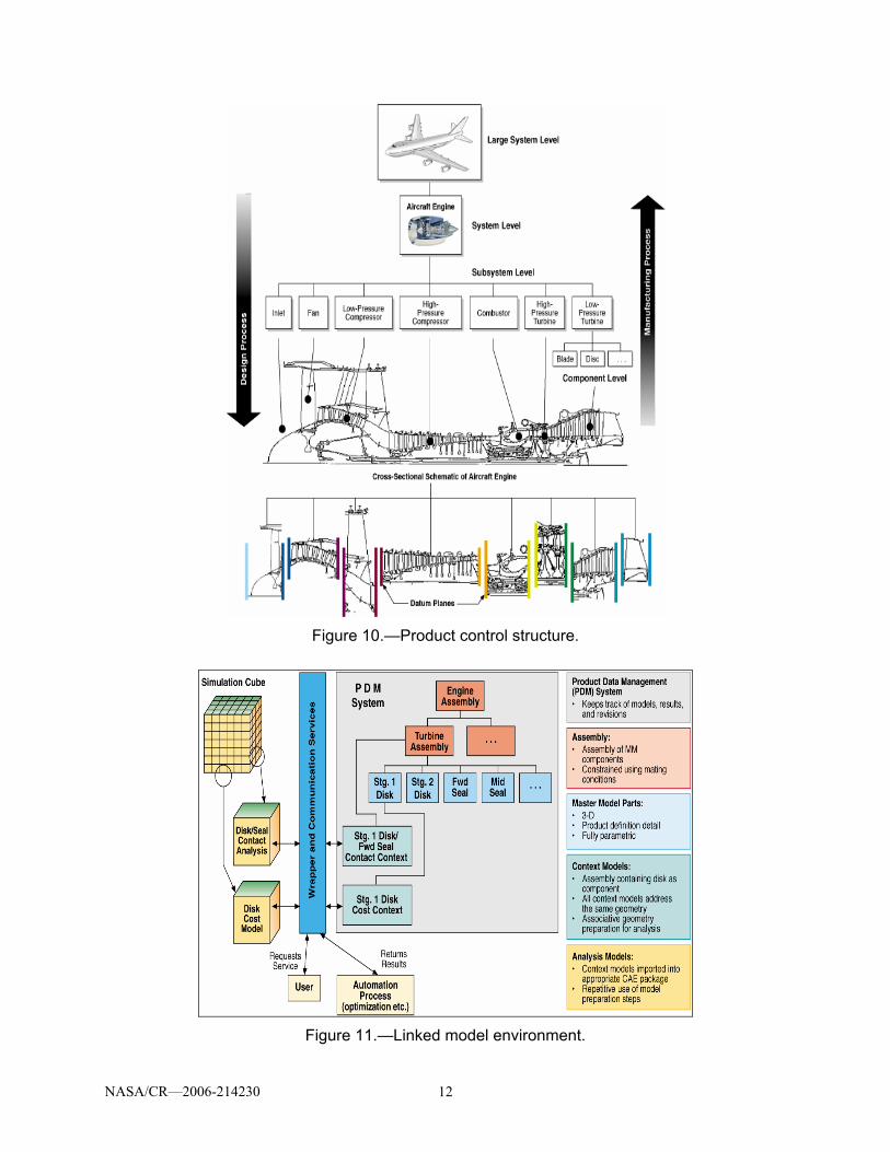
The effort to link geometry to NPSS draws extensively from several prior GE initiatives, primarily the Common Geometry Initiative and the System Oriented Layout and Integrated Design (SOLID) project. Concepts developed in these projects like the top-down Product Control Structure (PCS), (fig. 10), and the Linked Model Environment (LME), (fig. 11), form the backbone of the geometry structure used in this application of NPSS. These projects have been described in previous publications (refs. 5 and 6). Only key concepts are addressed here as necessary to understand this work. The primary objective of the Common Geometry initiative was the ability to use a common (evolving) geometry master model through the design and manufacturing process, so that at all times participants in the design and manufacturing process have access to the same geometry information. Taking advantage of the UNIGRAPHICS (UG) WAVE (UGS, Plano, TX) top-down geometry linking capability, a PCS for turbine engines was developed, specifying interfaces between the different engine subsystems and giving control of these interfaces to the groups responsible for system-level design. Each subsystem group owns its own interfaces between individual components.
NASA/CR—2006-214230 12
Figure 10.—Product control structure.
Figure 11.—Linked model environment.

NASA/CR—2006-214230 13
Understanding that different disciplinary engineering design and analysis tools require geometry at different levels of detail, the concept of a "context model" was introduced. The context model represents a disciplinary context-specific, yet fully associative, "view" of the master model geometry. Feature suppression is used in context models to create the desired view for a particular type of analysis. For example, a bolthole, which is important for stress analysis, may not be required for a thermal or CFD analysis and therefore could be suppressed in the thermal/fluids context model. These context models are then linked to the respective disciplinary analysis tools, e.g., FEA, CFD, cost, producibility, etc, in the LME, (see fig. 11).
Since its inception, the geometric master-model concept has been extended to the “Intelligent Master Model” (IMM) philosophy. Intelligence is added through use of Knowledge-Based Engineering (KBE) systems in the design process. Initially, rules for geometry generation were captured separately from the geometry itself. Later, with the addition of the Knowledge Fusion product into the UNIGRAPHICS CAD system (UG/Knowledge Fusion), this has become part of the IMM.
Geometry Morphing Geometry morphing is based on the ability to select a parametric part representation from a
library of parts and morph it based on high-level engine parameters and aero design information. The library geometry or the baseline geometry is selected and incorporated in the SOLID control structure along with flow information and design parameters.
At early design tollgates, aero design engineer calculates blade parameters such as the turning angles, solidity, pressure ratio as well as the overall geometry sizing parameters at the module level. The geometry morphing following this analysis has 3 main steps:
• Airfoil Morphing: The process starts off with identifying an airfoil from a library that can best achieve the flow conditions of the target airfoil. Typically, the library airfoils will be at the fidelity of either rig or production level of existing engines and would evolve as new parts are added. The cross sections of the library airfoils are morphed by a set of transfer functions (which are based on GE Aircraft Engine’s design rules) to attain the target blade radial extents, leading/trailing edge metal angles, chord, thickness and blade count. The resulting airfoil reflects the specified aero conditions with the implied mechanical details created from the selected baseline geometry by the morphing process. In the next step, this initial airfoil geometry will be swapped out with detailed blade geometry.
• Airfoil Reparenting: If a detailed design for the airfoil is available at any stage of the design, it can replace the initial morphed airfoil using a process called reparenting. Since the key interface dimensions and approximate shape are the same, the blade and disk mechanical analysis works the same with the original or new geometry. During a typical engine study, the preliminary morphed airfoils would first replace the library airfoil to get the multi-component mechanical design started and be finally replaced by a higher fidelity detailed airfoil.
• Disk/Attachment Resizing: The rule-based nature of the SOLID system would be used to calculate the dimensions of the disk and attachments that support the airfoil at the operating conditions.
In this work, NPSS dynamic linked modules were developed to query and modify the airfoil
aerodynamic conditions (consistent with NPSS cycle P & Ts) stored in a Global Data System (GDS – GEAE Aero Results Database) and subsequently to invoke the appropriate geometry morphing routines in UNIGRAPHICS to create the morphed airfoil geometry. To avoid the overhead delay in starting UG when geometry operations are performed, a server/client

NASA/CR—2006-214230 14
Figure 12.—NPSS Interface to geometry morphing routines.
architecture was developed in this work. UG was started in server mode and UG API calls were invoked from NPSS (see fig. 12). The concept of airfoil reparenting and disk resizing were implemented using UG API’s and Knowledge Fusion rules and were made available using NPSS DLM wrappers.
2.4 Compressor Mechanical Analysis
At the preliminary design stage, empirical estimates of airfoil root stresses and average dovetail stress can be arrived at from the flow conditions and low fidelity geometry. However, from the automatic geometric morphing using the SOLID control structure the designer can obtain a more detailed 3-D instance of a blade. The 3-D instance of a blade can be used to perform detailed ANSYS analysis that can give the PD engineer static and modal performance of the blade structure early on in the design process.
Blade Mechanical Analysis from NPSS During the engine design iterations, the SOLID control structure ensures that the geometric
model of the blade can be reused for mechanical analysis without the overhead of re-tagging entities in the part. Pitchline parameters such as the moment of circumferential velocity, pressure and temperature obtained from the BRM results executed within NPSS are used to scale the detailed pressure and temperature maps. The scaling can be based on design rules to ensure that the averaged values of resulting detailed map related quantities match the average pitch-line results. These rules were implemented as functions that can be called from the NPSS session. The next step is to trigger off the ANSYS run and post-process the results for the particular case.
2.5 A 500 nm Mission Fuel-Burn Roll-Up
Twin Engine HLTM Fuel-Burn Mission Study Here we consider a twin-engine aircraft mission study corresponding to a typical short-range
commercial aircraft with a 500 nm mission and a HLTM engine. The mission includes several climb segments until the aircraft reaches an altitude of 35000 ft and then a steady cruise segment and final descent phase. Figure 13 illustrates the results from a fuel-burn study conducted on this aircraft mission using two approaches: (1) Using an engine simulation with baseline estimates for HLTM compressor and turbine maps and associated uncertainty allowance. (2) Using the HLTM model results with map efficiency, map corrected flow and pressure ratio calculated using the BRM DLMs for each operating point. Comparisons are made at mid-altitude for each flight segment.

NASA/CR—2006-214230 15
Figure 13.—A 500 nm fuel burn mission study.
As can be seen from these preliminary results, there is about 3 percent improvement
(7177 lbs as compared to 6966 lbs using base NPSS) in overall fuel-burn estimate with the integration of BRM model with NPSS. This result should be considered qualitatively rather than quantitatively. The estimate for component performance uncertainty includes many assumptions. The choice to reduce actual design margin based on the improved confidence depends on both regulatory issues, internal design processes, business issues and judgment on other sources of uncertainty that are unrelated to design and analysis issues. The model and uncertainty used in this particular study were selected in conjunction with NASA to be representative and do not correspond to any GEAE engine.
High fidelity analysis feedback at early tollgates can identify potential problems early on when it is easy to accommodate design changes, in contrast to identifying these problems at a later stage of the engine design program where deadline pressures, previous commitments and expanding program effort make the cost of change very high. Addressing these issues provides support to the choice of whether to act on the reduced uncertainty to create a more optimum design or to simply reduce the program risk. In the following section, we present results from research efforts conducted under this contract to enable aerodynamic/aero-mechanical high-fidelity system simulation capabilities within the NPSS system. Efforts to improve confidence bounds on component high-fidelity simulations employing unsteady effects were also addressed as a part of this contract and will also be discussed in detail in the following sections.

NASA/CR—2006-214230 16
3.0 HLTM High Fidelity System Simulation 3.1 High Fidelity CFD Feedback to NPSS
Advances in the speed and availability of computer processors have enabled advanced two- and three-dimensional Computational Fluid Dynamics (CFD) based techniques to be applied to the design of turbomachinery components. Methods for simulating multistage turbomachinery have also been developed, and are now being regularly applied in the design process. While advanced numerical simulations of isolated components yielding detailed performance data at unique component operating points have been demonstrated, very little effort has been focused in using these high-fidelity simulations to update system models, wherein interactions between adjoining components is accounted for. Overall engine performance is dependent on the components working together very efficiently over a range of demanding operating conditions, and several components are sensitive to interactions with adjoining components. For example, compressor performance is very sensitive to steady inlet and outlet flow conditions, which is a function of the mechanisms in the adjoining components. As a result, it is important to consider the engine as a system of components that influence each other, and not simply isolated components.
Although performance maps attempt to capture component interactions, they lack the wealth of information embedded in a high-fidelity component CFD simulation, such as details of the shock mechanisms, boundary layer effects, etc. Flowing up this level of detail into a system model can prove very effective in improving the accuracy of these performance models. If there is sufficient confidence in the CFD results and if there is adequate CFD data available to provide sufficient coverage across the operating envelope, this approach can one day help reduce (or possibly even eliminate) the need for costly and time-consuming rig/engine tests. Towards this end, an approach was developed in the present work to flow-up CFD-level of detail into NPSS. The approach taken here is a “2-step” approach, wherein 1-D averaged CFD results at multiple operating points are used to improve the component map generation tool, BRM. This improved model, in turn, is plugged into the NPSS system to provide real-time access to accurate map information.
One of the challenges while working with CFD simulations is sometimes the overabundance of information embedded within these results. In using CFD results to update 1-D intermediate fidelity models, such as the Blade Row Model, an important step is to generate appropriate 1-D averages that can be correlated 1-to-1 with the corresponding variables in the intermediate fidelity model. The following section describes how these 1-D averaged variables are derived from detailed CFD results that satisfy all requirements of mass, momentum and energy conservation.
HLTM Compressor Map Data-Matching Example Here, we consider a typical HLTM engine with a 6-stage compressor. The BRM model
generates a compressor map such as the one shown in figure 6 using several empirical tuning factors, which need to be set to appropriate levels based on designer experience and physical insight. Some of these empirical factors include base loss coefficient, deviation slope factors, factors to account for high/low Mach number and flow separation effects, blockage coefficients, etc. Each of these empirical factors has an appropriate upper/lower bound, specified based on the underlying physics. There is a certain degree of fuzziness associated with these bounds, partly because of lack of deeper understanding of the physical mechanisms and partly due to the difficulty in obtaining validating test data. In this work, we apply the CFD-based averaging and data-matching techniques elaborated earlier to this example problem. Multiple operating points are employed in this study to provide sufficient coverage across the operating regime of

NASA/CR—2006-214230 17
the compressor. The various empirical parameters are tuned using an optimizer to minimize an objective.
A total of 52 empirical design variables were considered in this work. The objective of the study was to vary these empirical factors (within appropriate upper/lower bounds specified by the designer) so as to minimize the objective function.
Overall, this study has emphasized the use of a CFD-based approach to component map data-matching problems using an optimization/inverse problem framework. The results show that a good base match can be obtained using this proposed automated optimization-based approach. Here, the authors would like to emphasize that, while it is feasible to obtain a good base match using a completely automated optimization-based approach, final off-design matching requires a deeper understanding of the underlying physical mechanisms and requires some manual fine-tuning to adhere to design best practices.
3.2 Improved Component Simulations via Multi-Stage Unsteady CFD
The previous sections discussed about two related (but distinct) high-fidelity zooming efforts focused on flowing up high-fidelity analysis results (aerodynamic and aeromechanical results) to improve engine-level system uncertainty at early tollgates. The fundamental assumption in this philosophy is that the high-fidelity component analysis results are very accurate and match test conditions adequately. While this is generally the case, it is important to realize that these high-fidelity analysis codes have their inherent limitations and are constantly being improved using advanced physics-based models. For example, multi-stage CFD based component simulations used regularly in design these days is most often based on steady flow physics and do not capture physics associated with unsteady blade row interactions. The reason for using steady codes in multistage analysis is not that the technology doesn’t exist for unsteady multistage analysis, but rather, the large computing resources required. One of the goals of the present research was to evaluate the unsteady flow features occurring in a turbomachinery component (High Pressure Compressor in this case) by the use of a multistage unsteady flow simulation and demonstrate the feasibility of large unsteady multistage analysis via the use of massively parallel computing capabilities.
One of the typical multistage CFD analysis techniques places a mixing plane in the gap between the blade rows. The flow field is steady in the frame of reference of the current blade row and the unsteadiness from neighboring blade rows is averaged tangentially. Another method is by utilizing the average passage approach that is used in APNASA (refs. 10 and 11). In this method, body forces and deterministic stresses represent the neighboring blade rows and interaction effects. This method is more accurate than using a mixing plane, but it still neglects some physics associated with unsteady blade row interactions. Utilizing an unsteady code for multistage analysis removes the requirement to model interaction effects since they are computed directly. In this work, the unsteady CFD code MSU-TURBO (ref. 12) was used. This employs a sliding interface between the blade rows to take into account the unsteady effects. A GEAE 3-1/2 stage research compressor is the subject of the current study. It is representative of modern high stage loading, high-pressure ratio compressors. A cross section of the compressor is shown in figure 14. The unsteady CFD code MSU-TURBO was used to model the seven blade rows, the IGV (Inlet Guide Vane) through S3 (Stator 3). Less than 1/4 wheel was used instead of a full annulus to reduce the size of the calculation. At the tangential boundaries, periodicity was enforced at every time step. To obtain a periodic sector, the counts on all the blades except R2 were modified. The max thicknesses on S1-S3 were modified to maintain the same metal blockage. Variable vane end gaps were modeled, but no cavity leakages were included. The exit area was increased to account for the S3 exit bleed slot, by moving the case outward. The grid on each blade was a single block H mesh that was obtained from the code APG with 22 million grid points used for the entire simulation. A representative grid in the blade-

NASA/CR—2006-214230 18
Figure 14.—Cross-section of 3-1/2 stage research compressor.
LEDetail
TE Detail
IGV
Figure 15.—Typical single block mesh details (IGV shown).
to-blade plane is shown in figure 15. Each single block grid passage was decomposed into 256 blocks for parallel computing. Over the rotor tips, an open tip gap model was used with 12 cells clustered toward the casing (Van Zante et al., 2000). At the inlet, a steady flow radial profile was used holding radial flow angle, tangential flow angle, total pressure, total temperature, and turbulence quantities. At the exit, a static pressure profile was held, but the level was adjusted to hold exit corrected mass flow. The boundary conditions were derived from a data-match of the compressor at the design point, which is on the operating line. The simulation utilized 256 processors and 65.5 GB of memory on NASA’s SGI Origin 3800 supercomputer (CHAPMAN). The converged solution required 86666 CPU hours, which is equivalent to 14 days of continuous running. The simulation was run in stages to check to see if the solution was progressing without errors. In simulation time, the solution advanced one revolution of the wheel.
IGV R1 S1 R2 S2 R3 S3

NASA/CR—2006-214230 19
Results Convergence.—A primary check on convergence is the physical mass flow. For an
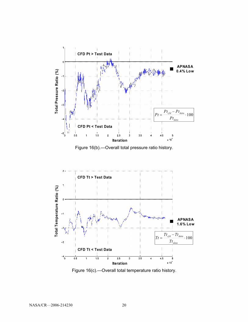
unsteady simulation, the time-averaged mass flow at the inlet and exit should be equivalent, but don’t necessarily have to be the same at each time step. Figure 16(a) shows the physical mass flow history at the inlet and exit of the compressor normalized by the experimental mass flow. The inlet and exit time-average flows are within 0.2 percent of the experimental data and each other. In addition, the APNASA simulation results are 0.3 percent higher than the data (black solid square in the figure). The convergence history of the total pressure ratio, total temperature ratio, and efficiency are also shown relative to the data. The total pressure ratio history (fig. 16(b)) shows good convergence and that the TURBO prediction is low by approximately 0.8 percent while the APNASA simulation is only 0.4 percent low. Total temperature is similar (fig. 16(c)), with TURBO and APNASA low by 1.25 and 1.6 percent, respectively. The low total temperature results in a high overall efficiency shown in figure 16(d) with TURBO and APNASA both high by 2.25 and 3.3 percent, respectively. Overall, the simulation showed good convergence. NASA personnel ran the simulation further resulting in very little change in the convergence. Individual stages also showed good convergence. An example of the mass flow history for Stator 1 and Rotor 2 is shown in figure 16(e). Notice the initial transients followed by steady time-averaged inlet and exit mass flows for the individual blade rows.
Ma s
s flo
w (%
)
Iteration
100⋅−
=data
datacfd
mmm
m&
&&&
CFD Masslow > Test Data
CFD Masslow < Test Data
Exit
Inlet
APNASA0.3% High
Figure 16(a).—Inlet and exit mass flow history relative to experimental data.
NASA/CR—2006-214230 20
100⋅−
=data
datacfd
PtPtPt
Pt
Iteration
Tota
l Pr e
s su r
e R
a tio
(%
)CFD Pt > Test Data
CFD Pt < Test Data
APNASA0.4% Low
Figure 16(b).—Overall total pressure ratio history.
Tot a
l Te m
pera
t ure
Ra t
i o (
%)
Iteration
100⋅−
=data
datacfd
TtTtTt
Tt
CFD Tt > Test Data
CFD Tt < Test Data
APNASA1.6% Low
Figure 16(c).—Overall total temperature ratio history.

NASA/CR—2006-214230 21
100⋅−
=data
datacfd
ηηη
η
Ad i
a ba t
i c E
ffic
ienc
y (%
)
Iteration
CFD Efficiency > Test Data
CFD Efficiency < Test Data
APNASA3.3% High
Figure 16(d).—Overall adiabatic efficiency history.
IterationIteration
Mas
sfl o
w (%
)
Ma s
s flo
w ( %
)
S1 Massflow R2 Massflow
S1 Exit
S1 Inlet
R2 Exit
R2 Inlet
Figure 16(e).—S1 and R2 individual mass flow history.
Stage Performance The stage-by-stage performance comparison between TURBO and APNASA gives clues on
the magnitude of the unsteady effects as it relates to performance and stage matching. The total pressure and total temperature ratios, and adiabatic efficiency difference between the two codes relative to APNASA is shown in table 1. A stage is defined as a stator followed by a rotor and the largest differences are highlighted in red. To help explain these differences, the rotor alone characteristics are shown in figure 17. In this figure, the results are normalized with respect to APNASA result).

NASA/CR—2006-214230 22
TABLE 1.—STAGE-BY-STAGE PERFORMANCE DIFFERENCE BETWEEN TURBO AND APNASA NORMALIZED BY THE APNASA RESULT.
-0.04%0.71%2.20%2 - S1-R2
-1.61%-0.28%-1.62%3 - S2-R3
-0.91%0.27%-0.36%IGV-S3
-0.25%-0.10%-0.47%1 - IGV-R1
Adiabatic Efficiency
Tt/TtPt/PtStage
-0.04%0.71%2.20%2 - S1-R2
-1.61%-0.28%-1.62%3 - S2-R3
-0.91%0.27%-0.36%IGV-S3
-0.25%-0.10%-0.47%1 - IGV-R1
Adiabatic Efficiency
Tt/TtPt/PtStage
100⋅−
=apnasa
apnasaturbodelta X
XXX
Pt/P
t
P t/P
t
P t/P
t
Rotor 1 Rotor 2 Rotor3
0.12%TURBO
APNASA0.31%
1.0%
0.5%
2.1 %
1 .3 %
Tt/T
t
Rotor1 Inlet Corr Flow
Tt/T
t
Rotor2 Inlet Corr Flow
Tt/T
t
Rotor3 Inlet Corr Flow
0.7%
0.3 %0 .1 %
TURBO 1% low in Corrected Speed
TURBO 0.3% high in Corrected Speed
TURBO 0.5% low in Corrected Speed
η = - 0.23% η = - 0.55% η = - 0.75%
Figure 17.—Rotor-alone characteristics normalized to APNASA results.
Stage 1.—Stage 1 shows almost no difference in performance between TURBO and
APNASA. The rotor alone comparison is good with the rotor efficiency difference identical to the stage results. Therefore, the TURBO results show that Rotor 1 is causing the lower efficiency and not the IGV. TURBO gives a slightly lower rotor corrected speed, which implies a lower choked flow and the rotor is running on a lower operating line.
Stage 2.—In Stage 2, TURBO shows a 2.2 percent larger total pressure ratio across the stage with the same efficiency. The total temperature ratio is also larger by less than a percent. Looking at the rotor alone characteristics, TURBO also shows the rotor throttled up by 2.1 percent relative to APNASA. The corrected flow is higher by 0.3 percent due to the higher rotor inlet corrected speed (0.3%). The rotor alone efficiency is 0.55 percent less efficient than

NASA/CR—2006-214230 23
the APNASA result, which means that S1 has less loss in TURBO than APNASA. The rotor is operating on a higher operating line in TURBO and is throttled up past peak efficiency.
Stage 3.—In Stage 3, TURBO has a 1.6 percent lower pressure ratio with nearly identical temperature ratio resulting in a 1.6 percent lower adiabatic efficiency compared to APNASA. The inlet corrected flow is lower by 1.0 percent which results in a lower Rotor 2 exit corrected flow and explains the throttled up Rotor 2. The rotor alone efficiency is only 0.75 percent lower in TURBO relative to APNASA, which means the remaining lower efficiency in Stage 3 is caused by Stator 2 loss, which further throttles Rotor 2.
Rotor 2 Analysis.—The higher-pressure ratio in Rotor 2 shown in the TURBO case can also be explained by looking at figure 18, which shows relative Mach number at the Rotor 2 exit. The APNASA simulation is on the upper right, and the TURBO simulation is at the bottom and shows one instant in time. It can be seen that there is a hub separation in the APNASA simulation, which is not evident in TURBO. Figure 19 shows Rotor 2 exit entropy. Notice the increased loss in the rotor tip flow that TURBO predicts relative to APNASA. Rotor 2 being throttled up by Stage 3 causes this. However, there is a difference in the tip model between the codes. While TURBO uses a periodic boundary above the blade, APNASA uses mystery physics. The differences on the simulation were not investigated. Notice also that the blade wakes at the hub have less entropy production in the TURBO simulation because the hub is not separated.
APNASA
TURBO
R2 exit hub separation
R2 exit weak flow
%12.2100 =⋅⎟⎠⎞
⎜⎝⎛
⎟⎠⎞
⎜⎝⎛−⎟
⎠⎞
⎜⎝⎛
=⎟⎠⎞
⎜⎝⎛
apnasa
apnasaturbo
delta
PtPt
PtPt
PtPt
PtPt
Figure 18.—Rotor 2 exit relative Mach number showing separation in the hub in the APNASA simulation.

NASA/CR—2006-214230 24
APNASA
TURBO
TURBO predictingLess Efficient Tip flow
APNASA predictingMore Efficient Tip Flow
Figure 19.—Rotor 2 exit entropy showing increase in entropy in Rotor 2 tip in TURBO.
Pressure and Temperature Non-Uniformities
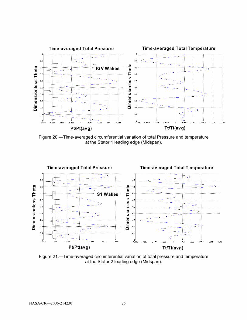
Unsteady simulations can also be used to help explain the variation that total pressure and temperature can have on measurements on stator leading edges. Figure 20 shows a midspan cut of the time-averaged total pressure and total temperature at Stator 1 leading edge as a function of angular position. They are normalized relative to the circumferentially averaged value. On the left in the figure, the low areas of total pressure shown are the IGV wakes. The other variations are the result of the Stator 1 potential field and also unsteady effects. The total temperature is shown on the right and displays a similar behavior. The Stator 2 total pressures and temperatures are shown in figure 21. Notice the S1 wakes. The other variations are from some interference with the IGV wakes, Stator 2 potential effects, and unsteady effects. To calculate interstage performance, the total pressures and temperatures are used. It is quite evident from these plots, that there could be large variations in the efficiency depending on where the stator leading edge probes are located. Stator leading edge probes are located such that previous stator wakes will not impact the probes. However, this cannot be guaranteed for all operating conditions and care must be taken in interpreting these measurements.
In an effort to quantify these effects a histogram was calculated by computing the efficiency at each circumferential point. The efficiency was calculated two ways. First, the total temperature was held constant at the average value and the efficiency was calculated only considering temperature variations. Next, the total pressure was held constant at the average value and the efficiency was calculated only considering pressure variations. The results are shown in figure 22 for the IGV-S2 as a representative case. Plotted is the number of occurrences, with the total number of occurrences being the total number of circumferential grid points as a function of normalized efficiency. The efficiency is normalized by the average efficiency. Notice that the efficiency can vary at least ±1 percent from the average level, which can be more than 1 point depending on the average.
NASA/CR—2006-214230 25
Time-averaged Total Pressure Time-averaged Total Temperature
Dim
ensi
onle
ss T
het a
Dim
ensi
onle
ss T
het a
Pt/Pt(avg) Tt/Tt(avg)
IGV Wakes
Figure 20.—Time-averaged circumferential variation of total Pressure and temperature
at the Stator 1 leading edge (Midspan).
S1 Wakes
Time-averaged Total Pressure Time-averaged Total Temperature
Dim
ensi
onl e
ss T
heta
Di m
ensi
onle
ss T
het a
Pt/Pt(avg) Tt/Tt(avg) Figure 21.—Time-averaged circumferential variation of total pressure and temperature
at the Stator 2 leading edge (Midspan).

NASA/CR—2006-214230 26
Occ
urr e
nces
Oc c
urr e
nce s
Time-averaged Total Temperature Held Time-averaged Total Pressure Held
Normalized Adiabatic Effic iency Normalized Adiabatic Efficiencyavgηη
avgηη
AVG AVG
Figure 22.—Histogram of circumferential IGV-S2 leading edge efficiency variation (Midspan).
Concluding Remarks A large multistage unsteady compressor simulation has been successfully demonstrated
using MSU TURBO on a 3-1/2 stage research compressor. TURBO was shown to run very well on massively parallel machines (256 processor demonstrated on this simulation). The simulation showed that unsteady flows cause differences in stage matching characteristics. Finally, post-processing of large unsteady simulations is very time consuming and costly in terms of storage.
Future plans for this work include the following. First, more analysis must be completed since only a small portion of the results have been analyzed to date. Next, the simulation should be continued to determine if solution has fully converged. Also, more operating points should be run to better determine the throttling characteristics of the stages and thus the stage characteristics. And lastly, the post-processing capability should continue to be developed to reduce time consuming post-processing.

NASA/CR—2006-214230 27
4.0 Uncertainty Metric Roll-Up In this final section, an assessment of the overall impact of this contract with regards to
bringing high fidelity system simulation capability within NPSS is presented. It is important to emphasize at this juncture that numerous assumptions have gone into this “quantitative” assessment. For this study the Fuel Burn (SFC) and Life (EGT Margin) have been the primary system-level metrics employed for comparing and trending the overall uncertainty improvements. By allowing system-level simulation capability at TG3 and bringing in high-fidelity analyses early on (typically, only available at TG6), the goal of this effort has been to lower the overall uncertainty at TG3 by approximately and approach that of TG6. The effort shown significant improvements over the existing capability in accuracy and uncertainty due to aero/mechanical/aero-mechanical zooming capability developed as a part of this contract. Due to programmatic constraints and restructuring at NASA, initially planned validation of these methodologies on UEET test configuration was subsequently dropped. It is estimated that this additional validation phase would have resulted in the same improvements to component models and the overall uncertainty metric. In the following discussion, we present the rationale (some qualitative) behind this overall metric assessment.
4.1 Uncertainty Reduction via High-Fidelity System Simulation at TG 3
Traditionally, several factors contribute to engine configuration uncertainty at Tollgate 3 from both geometry as well as analysis fronts. Some of these include:
Only FLOWPATH/WATE level of component definition is available during this stage Scaled/Parametric representation of component maps Secondary effects assessment is only historical in nature Mechanical analysis is only available at design conditions Analysis detail and accuracy is limited by the imposed boundary conditions Historical margins are used to maintain acceptable program risk Design trade-offs at component level are based on limited off-design conditions For HTML engines, there is an additional risk due to unavailability of engine-level
historical trends
The present effort has addressed several of these limitations by enabling high-fidelity analysis feedback within the NPSS framework. Some of these efforts include:
Automated creation of HLTM solid geometry from PD FLOWPATH level data Rig Detailed Geometry for Aero Assessment and Limited Detailed Mechanical Analysis Component Behavior at Key Point from High Fidelity Tools Validated by Rig Information Details from High Fidelity Tools used with Intermediate Fidelity Tools to Address
Barriers: • Setup Time • Boundary Conditions • Execution Speed • Configuration Changes • Range of Validity • Robustness
Direct modeling of secondary effects using intermediate fidelity tool level of empiricism Aero detail and boundary conditions at multiple flight conditions and power settings Mechanical analysis available and automated for range of parts, locations and operating
conditions

NASA/CR—2006-214230 28
Margins can be adjusted or risk reduced through direct assessment of system level design issues
HLTM risk assessed by greater confidence in analysis of cooling, mechanical and thermal pinch points
Direct use of Hi-Fi tools on HLTM issues such as Aeromechanics
As explained earlier in section 1.2, several factors contribute to uncertainty variation during design and development phases of an engine NPI program. These factors include technology improvements, design changes as well as test and measurement uncertainty. As shown conceptually in figure 23, overall uncertainty variation decreases significantly as the design matures from a concept (TG1/TRL1) to production roll out (TG9/TRL9). One of the main focus areas of this research contract has been to tightly integrate high-fidelity analysis (TG6) capability within NPSS system so that these design studies can be performed earlier in the design phase. Enabling such a system simulation capability not only streamlines the process and thereby improving overall design productivity, it also has a significant impact in terms of reducing the overall uncertainty at this stage (TG3/TRL4) of the design. This is explained in more detail in figure 24. As shown on the left, during a traditional TG3 phase the uncertainty in engine configuration is substantial, with the variation from the mean being substantial. In most engine programs, there is significant pressure to come up with customer quotes of EGT margin, SFC, etc at this phase (sometimes even as early as TG1/TRL1) and due to competitive/credibility issues it is important that these quotes be as close as possible to the final design numbers. However, due to design, test and measurement uncertainty at this phase of the design significant margin must be included in a possible quote. Now, on the right we can see the second scenario at TG6, wherein higher fidelity geometry as well as physics-based analysis helps reduce the uncertainty around the mean estimate. However, since many design decisions and critical choices must be made by TG3, this represents a lost opportunity. Having better estimates early can often help in coming in making the right choices, including “go” or “no-go” decisions on key features and technologies. This is exactly the problem this effort has attempted to address – Enabling system simulation capability within NPSS, to facilitate high-fidelity TG6 level analysis earlier in the design phase, thus improving overall confidence bounds on the predictions.
In the present context, risk is defined as any potential warranty or concession dollars. To be competitive and profitable, the engine manufacturer must provide the best possible engine while minimizing the overall program risks to avoid warranty and concessions costs associated with any miss in design guarantees. An “ideal” or “best” design quote at TG3 has significant risk. Extra margin is normally used to avoid warranty/concessions costs. At a reasonable confidence level, TG3-level analysis uncertainty represents a significant shift from the optimum engine and a loss of competitive advantage. By bringing in high fidelity system-simulation capability (with TG6 analysis capability plugged in), the uncertainty and risks are lowered. This can allow the same confidence level with a design much closer to the best configuration for the most likely engine. This reduction in margin without adding risk is the goal of this effort.

NASA/CR—2006-214230 29
10-1-2-3-4
Upper SpecLower Spec
sMean
0.87582-1.03800
Current Prediction Capability - TG#9 to TG#10
0.40.20.0-0.2-0.4
Upper SpecLower Spec
sMean
0.150.0
Production Variation
Mean 0.0S 0.15
210- 1- 2- 3- 4- 5- 6
U p p e r S p e cL o w e r S p e c
sM ea n
1 .33590-2 .373 33
C u r re n t P re d ic t io n C a p a b ility - T G # 7 to T G # 1 0
50- 5- 1 0- 1 5
U p p e rL o w e r
sM e a n
3 . 8 3 2 6 - 5 . 1 2 7 7
C u r r e n t P r e d i c t i o n C a p a b i l i t y - T G # 3 t o T G # 1 0
Production Variation
Prediction Variation TG#3 to TG#10
Prediction Variation TG#7 to TG#10
Prediction Variation TG#9 to TG#10
50- 5- 1 0- 1 5
U p p e rL o w e r
sM e a n
4 . 0 4 6 9 - 6 . 4 4 0 0
C u r r e n t P r e d i c t i o n C a p a b i l i t y - T G # 1 t o T G # 1 0
Prediction Variation TG#1 to TG#10
CommitmentCommitment
TG3/TRL4
TG6/TRL6
TG1/TRL1
TG9/TRL9
Production
SPECNOMINAL
Figure 23.—Uncertainty variation by engine tollgates.
85%
Engine Prediction Uncertainty
Pro
babi
lity
Prod. Var.
Pro
babi
lity
Extra Margin
Engine Prediction Uncertainty
Prod. Var.
Pro
babi
lity
Extra Margin
OrigTG3 Spec
Spec
TG3 Margins
SystemTrades
SystemTrades
Pro
babi
lity
TG6 Margins
85%
Orig 85%
Spec
85%
Engine Prediction Uncertainty
Pro
babi
lity
Prod. Var.
Pro
babi
lity
Extra Margin
Engine Prediction Uncertainty
Prod. Var.
Pro
babi
lity
Extra Margin
OrigTG3 Spec
Spec
TG3 Margins
SystemTrades
SystemTrades
Pro
babi
lity
TG6 Margins
85%
Orig 85%
Spec
Figure 24.—Uncertainty reduction via improved analysis capabilities.
NASA/CR—2006-214230 30
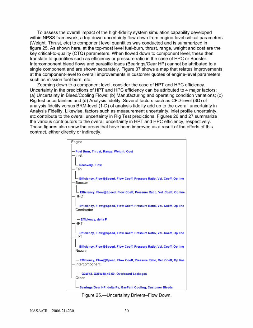
To assess the overall impact of the high-fidelity system simulation capability developed within NPSS framework, a top-down uncertainty flow-down from engine-level critical parameters (Weight, Thrust, etc) to component level quantities was conducted and is summarized in figure 25. As shown here, at the top-most level fuel-burn, thrust, range, weight and cost are the key critical-to-quality (CTQ) parameters. When flowed down to component level, these then translate to quantities such as efficiency or pressure ratio in the case of HPC or Booster. Intercomponent bleed flows and parasitic loads (Bearings/Gear HP) cannot be attributed to a single component and are shown separately. Figure 37 shows a map that relates improvements at the component-level to overall improvements in customer quotes of engine-level parameters such as mission fuel-burn, etc.
Zooming down to a component level, consider the case of HPT and HPC efficiency. Uncertainty in the predictions of HPT and HPC efficiency can be attributed to 4 major factors: (a) Uncertainty in Bleed/Cooling Flows; (b) Manufacturing and operating condition variations; (c) Rig test uncertainties and (d) Analysis fidelity. Several factors such as CFD-level (3D) of analysis fidelity versus BRM-level (1-D) of analysis fidelity add up to the overall uncertainty in Analysis Fidelity. Likewise, factors such as measurement uncertainty, inlet profile uncertainty, etc contribute to the overall uncertainty in Rig Test predictions. Figures 26 and 27 summarize the various contributors to the overall uncertainty in HPT and HPC efficiency, respectively. These figures also show the areas that have been improved as a result of the efforts of this contract, either directly or indirectly.
Fuel Burn, Thrust, Range, Weight, Cost
Recovery, Flow
Inlet
Efficiency, Flow@Speed, Flow Coeff, Pressure Ratio, Vel. Coeff, Op line
Fan
Efficiency, Flow@Speed, Flow Coeff, Pressure Ratio, Vel. Coeff, Op line
Booster
Efficiency, Flow@Speed, Flow Coeff, Pressure Ratio, Vel. Coeff, Op line
HPC
Efficiency, delta P
Combustor
Efficiency, Flow@Speed, Flow Coeff, Pressure Ratio, Vel. Coeff, Op line
HPT
Efficiency, Flow@Speed, Flow Coeff, Pressure Ratio, Vel. Coeff, Op line
LPT
Efficiency, Flow@Speed, Flow Coeff, Pressure Ratio, Vel. Coeff, Op line
Nozzle
G3W42, G26W48-49-50, Overboard Leakages
Intercomponent
Bearings/Gear HP, delta Ps, GasPath Cooling, Customer Bleeds
Other
Engine
Figure 25.—Uncertainty Drivers–Flow Down.

NASA/CR—2006-214230 31
Uncertainty in HPT Efficiency
Rig Tests
Measurement Uncertainty
Measurement to Analysis Uncertainty
Analysis Fidelity
Design Specifications
H41R (Energy Fn)
XN41R (Speed Fn)
BRM Uncertainty
Config. Changes
CFD Tip Clearance
Profile Variation
CFD <-> BRM Inconsistency
Bleeds/Cooling Flows
Vane NonChrg Cooling Flows
Blade Chrg Cooling Flows Other
ChargableCooling Flows
Mfg. & Operating Cond. Variations
Vane/Blade Surface Finish
Tip Clearances
Blade Contour
W41R (Flow Fn)
Data Matching
Limited Analysis Points
Limited Test Points
Vane/Blade TE Thickness
Inlet Profile Uncertainty
Component Interactions
Leakages Customer Bleeds
Blade Untwist
Vane Clocking
Not addressed under this effort
Direct High Fidelity Component effort
Direct High Fidelity Component effort
In-Direct High Fidelity Component effort
Uncertainty in HPT Efficiency
Rig Tests
Measurement Uncertainty
Measurement to Analysis Uncertainty
Analysis Fidelity
Design Specifications
H41R (Energy Fn)
XN41R (Speed Fn)
BRM Uncertainty
Config. Changes
CFD Tip Clearance
Profile Variation
CFD <-> BRM Inconsistency
Bleeds/Cooling Flows
Vane NonChrg Cooling Flows
Blade Chrg Cooling Flows Other
ChargableCooling Flows
Mfg. & Operating Cond. Variations
Vane/Blade Surface Finish
Tip Clearances
Blade Contour
W41R (Flow Fn)
Data Matching
Limited Analysis Points
Limited Test Points
Vane/Blade TE Thickness
Inlet Profile Uncertainty
Component Interactions
Leakages Customer Bleeds
Blade Untwist
Vane Clocking
Not addressed under this effort
Direct High Fidelity Component effort
Direct High Fidelity Component effort
In-Direct High Fidelity Component effort Figure 26.—HPT efficiency uncertainty drivers.
Uncertainty in HPT Efficiency
Rig Tests
Measurement Uncertainty
Measurement to Analysis Uncertainty
Analysis Fidelity
Design Specifications
Flow
Efficiency
BRM Uncertainty
Config. Changes
CFD Tip Clearance
Profile Effects
CFD <-> BRM Inconsistency
Bleeds/Cooling Flows
Inter-Stage Pressure/Temperature
Bleed Impact
n Performance VSV Impact
on Bleed
Mfg. & Operating Cond. Variations
Vane/Blade Surface Finish
Tip Clearances
Blade Contour
Pr
Data Matching
Limited Analysis Points
Limited Test Points
Vane/Blade TE Thickness
Inlet Profile Uncertainty
Component Interactions
Leakages Customer Bleeds
Blade Untwist
VSV Optimization
Not addressed under this effort
Direct High Fidelity Component effort
In-Direct High Fidelity Component effort
VSV Rigging
Figure 27.—HPC efficiency uncertainty drivers.

NASA/CR—2006-214230 32
In addition to uncertainty reduction, which has been the primary focus of this effort, the authors also foresee significant improvements to overall development time (productivity) as a by-product of this system simulation effort. Some of these benefits and associated trade-offs include:
Reduced Testing Reduced Rework o Identify pinch-points/constraints o Set appropriate margins
Confidence to proceed with long lead items Speed later development work o Reduced iterations o Analysis complete early – faster perturbation
Choice in setting margins o Reduce margin and hold risk o Maintain margins and reduce risk
Choice driven by business and customer program needs Must justify sunk costs of early high fidelity analysis

NASA/CR—2006-214230 33
5.0 Conclusions In summary, the RASER/UEET High Fidelity System Simulation effort has addressed
various important objectives to enable high-fidelity system simulation capability within the NPSS framework. The scope of this effort has been restricted to highly-loaded turbomachinery components, with particular focus on High Pressure Turbine (HPT) and High Pressure Compressor (HPC) components. Initial focus of the contract efforts was directed at developing and validating intermediate fidelity NPSS model using PD geometry for HLTM engine. This was subsequently extended to high-fidelity NPSS model by overlaying detailed geometry to validate CFD against rig data. Intermediate and High-Fidelity system simulation demonstrations through the duration of this contract included (1) Aero Intermediate Fidelity System Simulation using Blade Row Model (Compressor & Turbine) within NPSS; (2) Blade Mechanical Analysis and Automated Morphing in NPSS using automated SOLID connection; (3) Aero-Mechanical (Forced Response/Flutter) analysis capability in NPSS; and finally (4) Detailed 3D-CFD feedback to NPSS via update of intermediate fidelity models. Overall, this contract has demonstrated a significant improvement in the overall NPI uncertainty margins via the intermediate and high-fidelity system simulation capability developed as part of this contract efforts. In this effort, both “feed-forward” and “feedback” approaches of analysis zooming was employed to enable system simulation capability in NPSS. Both these approaches have certain benefits and applicability in terms of specific applications – “feedback” zooming allows the flow-up of information from high-fidelity analysis to be used to update the NPSS model results by forcing the NPSS solver to converge to high-fidelity analysis predictions. This approach is effective in improving the accuracy of the NPSS model; however, it can only be used in circumstances where there is a clear physics-based strategy to flow up the high-fidelity analysis results to update the NPSS system model. “Feed-forward” zooming approach is more broadly useful in terms of enabling detailed aero/thermal/mechanical analysis at early stages of design for a specified set of critical operating points and using these analysis results to drive design decisions early in the development process.
6.0 References 1. Lytle, J.K., The Numerical Propulsion System Simulation: An Overview, NASA/TM—2000-
209915. 2. Novak, R.A., Streamline curvature computing procedures for fluid flow problems, Trans.
ASME Journal of Engineering for Power, 478–490, 89, 1967. 3. Hall, E.J., Aerodynamic modeling of multistage compressor flow fields – Part I, ASME Paper
97–GT–344. 4. Hall, E.J., Aerodynamic modeling of multistage compressor flow fields – Part II, ASME
Paper 97–GT–345. 5. Röhl P.J.; Kolonay R.M. et al.: A Federated Intelligent Product Environment. Proceedings,
8th AIAA/USAF/NASA/ISSMO Symposium on Multidisciplinary Analysis and Optimization, Long Beach, CA, September 2000.
6. Röhl, P.J.; Kolonay R.M. et al.: Intelligent Compressor Design in a Network-Centric Environment. Proceedings, ASME Computers in Engineering Conference, Pittsburgh, PA, September 2001.
7. Kaipio, J., and Somersalo, E., Statistical and Computational Inverse Problems, Applied Mathematical Sciences, 160, Springer, 2005.
8. Fletcher, R., Practical Methods of Optimization, Wiley-Interscience, New York, 1987. 9. Luenberger, D.G., Optimization by Vector Space Methods, Wiley-Interscience, NY, 1990. 10. Adamczyk, J.J., Mulac, R.A., and Celestina, M.L., A Model for Closing the Inviscid Form of
the Average-Passage Equation System, Journal of Turbomachinery, 180–186, 108, 1986.

NASA/CR—2006-214230 34
11. Adamczyk, J.J., Aerodynamic Analysis of Multistage Turbomachinery Flows in Support of Aerodynamic Design, Journal of Turbomachinery, 189–217, 122(2), 2000.
12. Chen, J.P., and Briley, W.R., A Parallel Flow Slover for Unsteady Multiple Blade Row Turbomachinery Simulations, ASME–2001–GT–0348, June 2001.

This publication is available from the NASA Center for AeroSpace Information, 301–621–0390.
REPORT DOCUMENTATION PAGE
2. REPORT DATE
19. SECURITY CLASSIFICATION OF ABSTRACT
18. SECURITY CLASSIFICATION OF THIS PAGE
Public reporting burden for this collection of information is estimated to average 1 hour per response, including the time for reviewing instructions, searching existing data sources,gathering and maintaining the data needed, and completing and reviewing the collection of information. Send comments regarding this burden estimate or any other aspect of thiscollection of information, including suggestions for reducing this burden, to Washington Headquarters Services, Directorate for Information Operations and Reports, 1215 JeffersonDavis Highway, Suite 1204, Arlington, VA 22202-4302, and to the Office of Management and Budget, Paperwork Reduction Project (0704-0188), Washington, DC 20503.
NSN 7540-01-280-5500 Standard Form 298 (Rev. 2-89)Prescribed by ANSI Std. Z39-18298-102
Form Approved
OMB No. 0704-0188
12b. DISTRIBUTION CODE
8. PERFORMING ORGANIZATION REPORT NUMBER
5. FUNDING NUMBERS
3. REPORT TYPE AND DATES COVERED
4. TITLE AND SUBTITLE
6. AUTHOR(S)
7. PERFORMING ORGANIZATION NAME(S) AND ADDRESS(ES)
11. SUPPLEMENTARY NOTES
12a. DISTRIBUTION/AVAILABILITY STATEMENT
13. ABSTRACT (Maximum 200 words)
14. SUBJECT TERMS
17. SECURITY CLASSIFICATION OF REPORT
16. PRICE CODE
15. NUMBER OF PAGES
20. LIMITATION OF ABSTRACT
Unclassified Unclassified
Final Contractor Report
Unclassified
1. AGENCY USE ONLY (Leave blank)
10. SPONSORING/MONITORING AGENCY REPORT NUMBER
9. SPONSORING/MONITORING AGENCY NAME(S) AND ADDRESS(ES)
National Aeronautics and Space AdministrationWashington, DC 20546–0001
Available electronically at http://gltrs.grc.nasa.gov
April 2006
NASA CR—2006-214230
E–15477
WBS 984754.02.07.03NAS3–01135, Task Order #6
41
High Fidelity System Simulation of Multiple Components in Support of theUEET Program
Ronald C. Plybon, Allan VanDeWall, Rajiv Sampath,Mahadevan Balasubramaniam, Ramakrishna Mallina, and Rohinton Irani
Propulsion systems (aircraft)
Unclassified -UnlimitedSubject Category: 07
GE Aircraft EnginesOne Neumann WayCincinnati, Ohio 45215
Ronald C. Plybon and Allan VanDeWall, GE Aircraft Engine, One Neumann Way, Cincinnati, Ohio 45215;Rajiv Sampath, Mahadevan Balasubramaniam, Ramakrishna Mallina, and Rohinton Irani, GE Global Research Center,1 Research Circle, Niskayuna, New York 12309. Project manager, Clayton Meyers, Vehicle Systems Projects Office,Glenn Research Center, organization code PRV, 216–433–3882.
The High Fidelity System Simulation effort has addressed various important objectives to enable additional capabilitywithin the NPSS framework. The scope emphasized High Pressure Turbine and High Pressure Compressor components.Initial effort was directed at developing and validating intermediate fidelity NPSS model using PD geometry andextended to high-fidelity NPSS model by overlaying detailed geometry to validate CFD against rig data. Both "feed-forward" and feedback" approaches of analysis zooming was employed to enable system simulation capability in NPSS.These approaches have certain benefits and applicability in terms of specific applications—"feedback" zooming allowsthe flow-up of information from high-fidelity analysis to be used to update the NPSS model results by forcing the NPSSsolver to converge to high-fidelity analysis predictions. This apporach is effective in improving the accuracy of theNPSS model; however, it can only be used in circumstances where there is a clear physics-based strategy to flow up thehigh-fidelity analysis results to update the NPSS system model. "Feed-forward" zooming approach is more broadlyuseful in terms of enabling detailed analysis at early stages of design for a specified set of critical operating points andusing these analysis results to drive design decisions early in the development process.

