hierfstat: estimation and tests of hierarchical f-statistics

Package ‘hierfstat’November 17, 2021

Version 0.5-10

Date 2021-11-16

Title Estimation and Tests of Hierarchical F-Statistics

Author Jerome Goudet [aut, cre],Thibaut Jombart [aut],Zhian N. Kamvar [ctb],Eric Archer [ctb],Olivier Hardy [ctb]

Maintainer Jerome Goudet <[email protected]>

Imports ade4,adegenet,gaston,gtools,methods

Suggests ape, pegas, knitr, rmarkdown, testthat

Description Estimates hierarchical F-statistics from haploid ordiploid genetic data with any numbers of levels in the hierarchy, following thealgorithm of Yang (Evolution(1998), 52:950).Tests via randomisations the significanceof each F and variance components, using the likelihood-ratio statistics G(Goudet et al. (1996) <https://www.genetics.org/content/144/4/1933>).Estimates genetic diversity statisticsfor haploid and diploid genetic datasets in various formats, including inbreeding andcoancestry coefficients, and population specific F-statistics followingWeir and Goudet (2017) <https://www.genetics.org/content/206/4/2085>.

Depends R (>= 2.10)

License GPL (>= 2)

URL https://www.r-project.org, https://github.com/jgx65/hierfstat

BugReports https://github.com/jgx65/hierfstat/issues

VignetteBuilder knitr

RoxygenNote 7.1.1

NeedsCompilation no

Repository CRAN

Date/Publication 2021-11-17 13:40:02 UTC

1

https://www.genetics.org/content/144/4/1933


https://www.r-project.org

https://github.com/jgx65/hierfstat

https://github.com/jgx65/hierfstat/issues

2 R topics documented:

R topics documented:AIc . . . . . . . . . . . . . . . . . . . . . . . . . . . . . . . . . . . . . . . . . . . . . 3allele.count . . . . . . . . . . . . . . . . . . . . . . . . . . . . . . . . . . . . . . . . . 4allelic.richness . . . . . . . . . . . . . . . . . . . . . . . . . . . . . . . . . . . . . . . 5basic.stats . . . . . . . . . . . . . . . . . . . . . . . . . . . . . . . . . . . . . . . . . . 6beta.dosage . . . . . . . . . . . . . . . . . . . . . . . . . . . . . . . . . . . . . . . . . 8betas . . . . . . . . . . . . . . . . . . . . . . . . . . . . . . . . . . . . . . . . . . . . . 9biall2dos . . . . . . . . . . . . . . . . . . . . . . . . . . . . . . . . . . . . . . . . . . . 11boot.ppbetas . . . . . . . . . . . . . . . . . . . . . . . . . . . . . . . . . . . . . . . . . 12boot.ppfis . . . . . . . . . . . . . . . . . . . . . . . . . . . . . . . . . . . . . . . . . . 13boot.ppfst . . . . . . . . . . . . . . . . . . . . . . . . . . . . . . . . . . . . . . . . . . 14boot.vc . . . . . . . . . . . . . . . . . . . . . . . . . . . . . . . . . . . . . . . . . . . 15cont.isl . . . . . . . . . . . . . . . . . . . . . . . . . . . . . . . . . . . . . . . . . . . . 16cont.isl99 . . . . . . . . . . . . . . . . . . . . . . . . . . . . . . . . . . . . . . . . . . 17crocrussula . . . . . . . . . . . . . . . . . . . . . . . . . . . . . . . . . . . . . . . . . 17diploid . . . . . . . . . . . . . . . . . . . . . . . . . . . . . . . . . . . . . . . . . . . . 18exhier . . . . . . . . . . . . . . . . . . . . . . . . . . . . . . . . . . . . . . . . . . . . 19fs.dosage . . . . . . . . . . . . . . . . . . . . . . . . . . . . . . . . . . . . . . . . . . 19fstat2dos . . . . . . . . . . . . . . . . . . . . . . . . . . . . . . . . . . . . . . . . . . . 21g.stats . . . . . . . . . . . . . . . . . . . . . . . . . . . . . . . . . . . . . . . . . . . . 22g.stats.glob . . . . . . . . . . . . . . . . . . . . . . . . . . . . . . . . . . . . . . . . . 23genet.dist . . . . . . . . . . . . . . . . . . . . . . . . . . . . . . . . . . . . . . . . . . 24genind2hierfstat . . . . . . . . . . . . . . . . . . . . . . . . . . . . . . . . . . . . . . . 26genot2al . . . . . . . . . . . . . . . . . . . . . . . . . . . . . . . . . . . . . . . . . . . 27getal . . . . . . . . . . . . . . . . . . . . . . . . . . . . . . . . . . . . . . . . . . . . . 28getal.b . . . . . . . . . . . . . . . . . . . . . . . . . . . . . . . . . . . . . . . . . . . . 28grm2kinship . . . . . . . . . . . . . . . . . . . . . . . . . . . . . . . . . . . . . . . . . 29gtrunchier . . . . . . . . . . . . . . . . . . . . . . . . . . . . . . . . . . . . . . . . . . 30hierfstat . . . . . . . . . . . . . . . . . . . . . . . . . . . . . . . . . . . . . . . . . . . 31ind.count . . . . . . . . . . . . . . . . . . . . . . . . . . . . . . . . . . . . . . . . . . 32indpca . . . . . . . . . . . . . . . . . . . . . . . . . . . . . . . . . . . . . . . . . . . . 32kinship2dist . . . . . . . . . . . . . . . . . . . . . . . . . . . . . . . . . . . . . . . . . 33kinship2grm . . . . . . . . . . . . . . . . . . . . . . . . . . . . . . . . . . . . . . . . . 34kinshipShift . . . . . . . . . . . . . . . . . . . . . . . . . . . . . . . . . . . . . . . . . 35mat2vec . . . . . . . . . . . . . . . . . . . . . . . . . . . . . . . . . . . . . . . . . . . 35matching . . . . . . . . . . . . . . . . . . . . . . . . . . . . . . . . . . . . . . . . . . 36ms2bed . . . . . . . . . . . . . . . . . . . . . . . . . . . . . . . . . . . . . . . . . . . 37ms2dos . . . . . . . . . . . . . . . . . . . . . . . . . . . . . . . . . . . . . . . . . . . 37nb.alleles . . . . . . . . . . . . . . . . . . . . . . . . . . . . . . . . . . . . . . . . . . 38pairwise.betas . . . . . . . . . . . . . . . . . . . . . . . . . . . . . . . . . . . . . . . . 38pairwise.neifst . . . . . . . . . . . . . . . . . . . . . . . . . . . . . . . . . . . . . . . . 39pairwise.WCfst . . . . . . . . . . . . . . . . . . . . . . . . . . . . . . . . . . . . . . . 40pcoa . . . . . . . . . . . . . . . . . . . . . . . . . . . . . . . . . . . . . . . . . . . . . 41pi.dosage . . . . . . . . . . . . . . . . . . . . . . . . . . . . . . . . . . . . . . . . . . 42pop.freq . . . . . . . . . . . . . . . . . . . . . . . . . . . . . . . . . . . . . . . . . . . 42pp.fst . . . . . . . . . . . . . . . . . . . . . . . . . . . . . . . . . . . . . . . . . . . . 43pp.sigma.loc . . . . . . . . . . . . . . . . . . . . . . . . . . . . . . . . . . . . . . . . . 44

AIc 3

print.pp.fst . . . . . . . . . . . . . . . . . . . . . . . . . . . . . . . . . . . . . . . . . . 44qn2.read.fstat . . . . . . . . . . . . . . . . . . . . . . . . . . . . . . . . . . . . . . . . 45read.fstat . . . . . . . . . . . . . . . . . . . . . . . . . . . . . . . . . . . . . . . . . . . 46read.fstat.data . . . . . . . . . . . . . . . . . . . . . . . . . . . . . . . . . . . . . . . . 47read.ms . . . . . . . . . . . . . . . . . . . . . . . . . . . . . . . . . . . . . . . . . . . 48read.VCF . . . . . . . . . . . . . . . . . . . . . . . . . . . . . . . . . . . . . . . . . . 49samp.between . . . . . . . . . . . . . . . . . . . . . . . . . . . . . . . . . . . . . . . . 50samp.between.within . . . . . . . . . . . . . . . . . . . . . . . . . . . . . . . . . . . . 51samp.within . . . . . . . . . . . . . . . . . . . . . . . . . . . . . . . . . . . . . . . . . 51sexbias.test . . . . . . . . . . . . . . . . . . . . . . . . . . . . . . . . . . . . . . . . . 52sim.freq . . . . . . . . . . . . . . . . . . . . . . . . . . . . . . . . . . . . . . . . . . . 53sim.genot . . . . . . . . . . . . . . . . . . . . . . . . . . . . . . . . . . . . . . . . . . 53sim.genot.metapop.t . . . . . . . . . . . . . . . . . . . . . . . . . . . . . . . . . . . . . 54sim.genot.t . . . . . . . . . . . . . . . . . . . . . . . . . . . . . . . . . . . . . . . . . . 56subsampind . . . . . . . . . . . . . . . . . . . . . . . . . . . . . . . . . . . . . . . . . 58TajimaD.dosage . . . . . . . . . . . . . . . . . . . . . . . . . . . . . . . . . . . . . . . 59test.between . . . . . . . . . . . . . . . . . . . . . . . . . . . . . . . . . . . . . . . . . 59test.between.within . . . . . . . . . . . . . . . . . . . . . . . . . . . . . . . . . . . . . 60test.g . . . . . . . . . . . . . . . . . . . . . . . . . . . . . . . . . . . . . . . . . . . . . 61test.within . . . . . . . . . . . . . . . . . . . . . . . . . . . . . . . . . . . . . . . . . . 62theta.Watt.dosage . . . . . . . . . . . . . . . . . . . . . . . . . . . . . . . . . . . . . . 63varcomp . . . . . . . . . . . . . . . . . . . . . . . . . . . . . . . . . . . . . . . . . . . 63varcomp.glob . . . . . . . . . . . . . . . . . . . . . . . . . . . . . . . . . . . . . . . . 65vec2mat . . . . . . . . . . . . . . . . . . . . . . . . . . . . . . . . . . . . . . . . . . . 66wc . . . . . . . . . . . . . . . . . . . . . . . . . . . . . . . . . . . . . . . . . . . . . . 67write.bayescan . . . . . . . . . . . . . . . . . . . . . . . . . . . . . . . . . . . . . . . 68write.fstat . . . . . . . . . . . . . . . . . . . . . . . . . . . . . . . . . . . . . . . . . . 68write.ped . . . . . . . . . . . . . . . . . . . . . . . . . . . . . . . . . . . . . . . . . . 69write.struct . . . . . . . . . . . . . . . . . . . . . . . . . . . . . . . . . . . . . . . . . 70yangex . . . . . . . . . . . . . . . . . . . . . . . . . . . . . . . . . . . . . . . . . . . . 71

Index 72

AIc Calculates corrected Assignment Index

Description

Calculates corrected Assignment Index as described in Goudet etal. (2002)

Usage

AIc(dat)

Arguments

dat a data frane with nlocs+1 columns,

https://onlinelibrary.wiley.com/doi/abs/10.1046/j.1365-294X.2002.01496.x

4 allele.count

Value

aic The corrected assignment index of each individual

Author(s)

Jerome Goudet <[email protected]>

References

Goudet J, Perrin N, Waser P (2002) Tests for sex-biased dispersal using bi-parentally inheritedgenetic markers 11, 1103:1114

allele.count Allelic counts

Description

Counts the number of copies of the different alleles at each locus and population

Usage

allele.count(data,diploid=TRUE)

Arguments

data A data frame containing the population of origin in the first column and thegenotypes in the following ones

diploid Whether the data are from diploid individuals

Value

A list of tables, –each with np (number of populations) columns and nl (numberof loci) rows– of the count of each allele

Author(s)


Examples

data(gtrunchier)allele.count(gtrunchier[,-2])


allelic.richness 5

allelic.richness Estimates allelic richness

Description

Estimates allelic richness, the rarefied allelic counts, per locus and population

Usage

allelic.richness(data,min.n=NULL,diploid=TRUE)

Arguments

data A data frame, with as many rows as individuals. The first column contains thepopulation to which the individual belongs, the following to the different loci

min.n The number of alleles down to which the number of alleles should be rar-efied. The default is the minimum number of individuals genotyped (times 2for diploids)

diploid a boolean specifying wether individuals are diploid (default) or haploid

Value

min.all The number of alleles used for rarefaction

Ar A table with as many rows as loci and columns as populations containing therarefied allele counts

Author(s)


References

El Mousadik A. and Petit R.J. (1996) High level of genetic differentiation for allelic richness amongpopulations of the argan tree argania spinosa skeels endemic to Morocco. Theoretical and AppliedGenetics, 92:832-839

Hurlbert S.H. (1971) The nonconcept of species diversity: a critique and alternative parameters.Ecology, 52:577-586

Petit R.J., El Mousadik A. and Pons O. (1998) Identifying populations for conservation on the basisof genetic markers. Conservation Biology, 12:844-855

Examples

data(gtrunchier)allelic.richness(gtrunchier[,-1])

6 basic.stats

basic.stats Basic diversity and differentiation statistics

Description

Estimates individual counts, allelic frequencies, observed heterozygosities and genetic diversitiesper locus and population. Also Estimates mean observed heterozygosities, mean gene diversitieswithin population Hs, Gene diversities overall Ht and corrected Htp, and Dst, Dstp. Finally, esti-mates Fst and Fstp as well as Fis following Nei (1987) per locus and overall loci

Usage

basic.stats(data,diploid=TRUE,digits=4)

## S3 method for class 'basic.stats'print(x,...)

Hs(data,...)

Ho(data,...)

Arguments

data a data frame where the first column contains the population to which the differ-ent individuals belong, and the following columns contain the genotype of theindividuals -one locus per column-

diploid Whether individuals are diploids (default) or haploidsdigits how many digits to print out in the output (default is 4)x an object of class basic.stats... further arguments to pass to print.bas.stats

Value

n.ind.samp A table –with np (number of populations) columns and nl (number of loci) rows–of genotype counts

pop.freq A list containing allele frequencies. Each element of the list is one locus. Foreach locus, Populations are in columns and alleles in rows

Ho A table –with np (number of populations) columns and nl (number of loci) rows–of observed heterozygosities

Hs A table –with np (number of populations) columns and nl (number of loci) rows–of observed gene diversities

Fis A table –with np (number of populations) columns and nl (number of loci) rows–of observed Fis

perloc A table –with as many rows as loci– containing basic statistics Ho, Hs, Ht, Dst,Ht’, Dst’, Fst, Fst’ ,Fis, Dest

overall Basic statistics averaged over loci

basic.stats 7

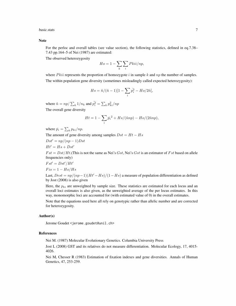
Note

For the perloc and overall tables (see value section), the following statistics, defined in eq.7.38–7.43 pp.164–5 of Nei (1987) are estimated:

The observed heterozygosityHo = 1−

∑k

∑i

Pkii/np,

where Pkii represents the proportion of homozygote i in sample k and np the number of samples.

The within population gene diversity (sometimes misleadingly called expected heterozygosity):

Hs = n/(n− 1)[1−∑i

p2i −Ho/2n],

where n = np/∑

k 1/nk and p2i =∑

k p2ki/np

The overall gene diversity

Ht = 1−∑i

pi2 +Hs/(nnp)−Ho/(2nnp),

where pi =∑

k pki/np.

The amount of gene diversity among samples Dst = Ht−HsDst′ = np/(np− 1)Dst

Ht′ = Hs+Dst′

Fst = Dst/Ht.(This is not the same as Nei’sGst, Nei’sGst is an estimator of Fst based on allelefrequencies only)

Fst′ = Dst′/Ht′

Fis = 1−Ho/HsLast, Dest = np/(np−1)(Ht′−Hs)/(1−Hs) a measure of population differentiation as definedby Jost (2008) is also given

Here, the pki are unweighted by sample size. These statistics are estimated for each locus and anoverall loci estimates is also given, as the unweighted average of the per locus estimates. In thisway, monomorphic loci are accounted for (with estimated value of 0) in the overall estimates.

Note that the equations used here all rely on genotypic rather than allelic number and are correctedfor heterozygosity.

Author(s)


References

Nei M. (1987) Molecular Evolutionary Genetics. Columbia University Press

Jost L (2008) GST and its relatives do not measure differentiation. Molecular Ecology, 17, 4015-4026.

Nei M, Chesser R (1983) Estimation of fixation indexes and gene diversities. Annals of HumanGenetics, 47, 253-259.

8 beta.dosage

See Also

ind.count,pop.freq.

Examples

data(gtrunchier)basic.stats(gtrunchier[,-1])Hs(gtrunchier[,-2])Ho(gtrunchier[,-2])

beta.dosage Estimates pairwise kinships and individual inbreeding coefficientsfrom dosage data

Description

Estimates pairwise kinships (coancestries) and individual inbreeding coefficient using Weir andGoudet (2017) beta estimator.

Usage

beta.dosage(dos,inb=TRUE,Mb=FALSE,MATCHING=FALSE)

Arguments

dos A matrix of 0, 1 and 2s with loci (SNPs) in columns and individuals in rows.Missing values are allowed

inb whether individual inbreeding coefficient should be estimated (rather than self-coancestries)

Mb whether to output the mean matching

MATCHING if MATCHING=FALSE, dos is a (ni x nl) dosage matrix; if MATCHING=TRUE, dos is a(ni x ni) matrix of matching proportions, as obtained from a call to the matchingfunction

Details

This function is written for dosage data, i.e., how many doses of an allele (0, 1 or 2) an individualcarries. It should be use for bi-allelic markers only (e.g. SNPs), although you might "force" a kmultiallelic locus to k biallelic loci (see fstat2dos).

Matching proportions can be obtained by the following equation: M = β ∗ (1−Mb) +Mb

By default (inb=TRUE) the inbreeding coefficient is returned on the main diagonal. With inb=FALSE,self coancestries are reported.

Twice the betas with self-coancestries on the diagonal gives the Genomic Relationship Matrix(GRM)

Following a suggestion from Olivier Hardy, missing data are removed from the estimation proce-dure, rather than imputed (this is taken care off automatically)

betas 9

Value

if Mb=FALSE, a matrix of pairwise kinships and inbreeding coefficients (if inb=TRUE) or self-coancestries (inb=FALSE); if Mb=TRUE, a list with elements inb (whether inbreeding coefficientsrather than kinships should be returned on the main diagonal), MB (the average off-diagonal match-ing) and betas the kinships or inbreeding coefficients.

Author(s)


References

Weir, BS and Goudet J. 2017 A Unified Characterization of Population Structure and Relatedness.Genetics (2017) 206:2085

Goudet, J., Kay, T. and Weir BS. 2018 How to estimate kinship. Molecular Ecology 27:4121.

Examples

## Not run:dos<-matrix(sample(0:2,size=10000,replace=TRUE),ncol=100)beta.dosage(dos,inb=TRUE)

#matrix of kinship/inbreeding coeffdata(gtrunchier)beta.dosage(fstat2dos(gtrunchier[,-c(1:2)]))

#individual inbreeding coefficientsdat<-sim.genot(size=100,nbloc=100,nbal=20,mig=0.01,f=c(0,0.3,0.7))hist(diag(beta.dosage(fstat2dos(dat[,-1]))),breaks=-10:100/100,main="",xlab="",ylab="")abline(v=c(0.0,0.3,0.7),col="red")#only 20 locihist(diag(beta.dosage(fstat2dos(dat[,2:21]))),breaks=-5:20/20,main="",xlab="",ylab="")abline(v=c(0.0,0.3,0.7),col="red")

## End(Not run)

betas Estimates βs per population and a bootstrap confidence interval

Description

Estimate populations (Population specific FST) or individual coancestries and a bootstrap confi-dence interval, assuming random mating


https://onlinelibrary.wiley.com/doi/full/10.1111/mec.14833

10 betas

Usage

betas(dat,nboot=0,lim=c(0.025,0.975),diploid=TRUE,betaijT=FALSE)

## S3 method for class 'betas'print(x, digits = 4, ...)

Arguments

dat data frame with genetic data and pop identifier

nboot number of bootstrap samples.

lim width of the bootstrap confidence interval

diploid whether the data comes from a diploid organism

betaijT whether to estimate individual coancestries

x a betas object

digits number of digits to print

... further arguments to pass to print

Details

If betaijT=TRUE, and the first column contains a unique identifier for each individual, the functionreturns the matrix of individual coancestries/kinships. Individual inbreeding coefficients can beobtained by multiplying by 2 the diagonal and substracting 1.

Value

Hi Within population gene diversities (complement to 1 of matching probabilities)

Hb Between populations gene diversities

betaiovl Average ˆβiWT over loci (Population specific FSTs), Table 3 of Weir and Goudet, 2017

(Genetics)

betaW Average of the betaiovl ˆβWT over loci (overall population FST)

ci The bootstrap confidence interval of population specific FSTs (only if more than 100 bootstrapsrequested AND if more than 10 loci are present)

if betaijT=TRUE, return the matrix of pairwise kinships only.

Methods (by generic)

• print: print function for betas class

Author(s)


References

Weir and Goudet, 2017 (Genetics) A unified characterization of population structure and related-ness.




biall2dos 11

See Also

fs.dosage, beta.dosage for Fst estimates (not assuming Random Mating) and kinship estimatesfrom dosage data, respectively

Examples

## Not run:#3 different population sizes lead to 3 different betaisdat<-sim.genot(size=40,N=c(50,200,1000),nbloc=50,nbal=10)betas(dat,nboot=100)

#individual coancestries from the smallest population are largeind.coan<-betas(cbind(1:120,dat[,-1]),betaij=T)diag(ind.coan$betaij)<-NAgraphics::image(1:120,1:120,ind.coan$betaij,xlab="Inds",ylab="Inds")

## End(Not run)

biall2dos Converts bi-allelic SNPs from hierfstat format to dosage format

Description

Converts bi-allelic SNPs hierfstat format to dosage format, the number of alternate allele copies ata locus for an individual, i.e. 11 -> 0; 12 or 21 >1 and 22 ->2

Usage

biall2dos(dat,diploid=TRUE)

Arguments

dat a hierfstat data frame without the first column (the population identifier), indi-viduals in rows, columns with individual genotypes encoded as 11, 12, 21 and22

diploid whether the data set is from a diploid organism

Value

a matrix containing allelic dosages

Examples

## Not run:biall2dos(sim.genot(nbal=2,nbloc=10)[,-1]) # a 10 column matrix

## End(Not run)

12 boot.ppbetas

boot.ppbetas Estimates bootstrap confidence intervals for pairwise betas FST esti-mates

Description

Estimates bootstrap confidence intervals for pairwise betas FST estimates.

Usage

boot.ppbetas(dat=dat,nboot=100,quant=c(0.025,0.975),diploid=TRUE,digits=4)

Arguments

dat A data frame containing population of origin as the first column and multi-locusgenotypes in following columns

nboot the number of bootstrap samples to draw

quant the limit of the confidence intervals

diploid whether the data is from a diploid (default) or haploid organism

digits how many digits to print out

Value

a matrix with upper limit of the bootstrap CI above the diagonal and lower limit below the diagonal

See Also

betas pairwise.betas

Examples

## Not run:data(gtrunchier)boot.ppbetas(gtrunchier[,-2])

## End(Not run)

boot.ppfis 13

boot.ppfis Performs bootstrapping over loci of population’s Fis

Description

Performs bootstrapping over loci of population’s Fis

Usage

boot.ppfis(dat=dat,nboot=100,quant=c(0.025,0.975),diploid=TRUE,dig=4,...)

Arguments

dat a genetic data frame

nboot number of bootstraps

quant quantiles

diploid whether diploid data

dig digits to print

... further arguments to pass to the function

Value

call function call

fis.ci Bootstrap ci of Fis per population

Author(s)


Examples

dat<-sim.genot(nbpop=4,nbloc=20,nbal=10,f=c(0,0.2,0.4,0.6))boot.ppfis(dat)

14 boot.ppfst

boot.ppfst Performs bootstrapping over loci of pairwise Fst

Description

Performs bootstrapping over loci of pairwise Fst

Usage

boot.ppfst(dat=dat,nboot=100,quant=c(0.025,0.975),diploid=TRUE,...)

Arguments


nboot number of bootstraps

quant the quantiles for bootstrapped ci

diploid whether data are from diploid organisms


Value

call call to the function

ll lower limit ci

ul upper limit ci

vc.per.loc for each pair of population, the variance components per locus

Author(s)


Examples

data(gtrunchier)x<-boot.ppfst(gtrunchier[,-2])x$llx$ul

boot.vc 15

boot.vc Bootstrap confidence intervals for variance components

Description

Provides a bootstrap confidence interval (over loci) for sums of the different variance components(equivalent to gene diversity estimates at the different levels), and the derived F-statistics, as sug-gested by Weir and Cockerham (1984). Will not run with less than 5 loci. Raymond and Rousset(199X) points out shortcomings of this method.

Usage

boot.vc(levels=levels,loci=loci,diploid=TRUE,nboot=1000,quant=c(0.025,0.5,0.975))

Arguments

levels a data frame containing the different levels (factors) from the outermost (e.g.region) to the innermost before the individual

loci a data frame containing the different loci

diploid Specify whether the data are coming from diploid or haploid organisms (diploidis the default)

nboot Specify the number of bootstrap to carry out. Default is 1000

quant Specify which quantile to produce. Default is c(0.025,0.5,0.975) giving the per-centile 95% CI and the median

Value

boot a data frame with the bootstrapped variance components. Could be used forobtaining bootstrap ci of statistics not listed here.

res a data frame with the bootstrap derived statistics. H stands for gene diversity, Ffor F-statistics

ci Confidence interval for each statistic.

References

Raymond M and Rousset F, 1995. An exact test for population differentiation. Evolution. 49:1280-1283

Weir, B.S. (1996) Genetic Data Analysis II. Sinauer Associates.

Weir BS and Cockerham CC, 1984. Estimating F-statistics for the analysis of population structure.Evolution 38:1358-1370.

See Also

varcomp.glob.

16 cont.isl

Examples

#load data setdata(gtrunchier)boot.vc(gtrunchier[,c(1:2)],gtrunchier[,-c(1:2)],nboot=100)

cont.isl A genetic dataset from a diploid organism in a continent-island model

Description

A simple diploid dataset, with allele encoded as one digit number. Up to 4 alleles per locus

Usage

data(cont.isl)

Format

A data frame with 150 rows and 6 columns:

Pop Population identifier, from 1 to 3

loc.1 genotype at loc.1





...

Source

generated with function sim.genot()

Examples

data(cont.isl)allele.count(cont.isl)

cont.isl99 17

cont.isl99 A genetic dataset from a diploid organism in a continent-island model

Description

A simple diploid dataset, with alleles encoded as two digits numbers. Up to 99 alleles per locus

Usage

data(cont.isl99)

Format







loc.5 genotype at loc.5...

Source

generated with function sim.genot(nbal=99)

Examples

data(cont.isl99)allele.count(cont.isl99)

crocrussula Genotypes and sex of 140 shrews Crocidura russula

Description

A dataset containing microsatellite genotypes, population and sex of 140 Crocidura russula individ-uals

Usage

data(crocrussula)

18 diploid

References

Favre et al. (1997) Female-biased dispersal in the monogamous mammal Crocidura russula: evi-dence from field data and microsatellite patterns. Proceedings of the Royal Society, B (264): 127-132


Examples

data(crocrussula)aic<-AIc(crocrussula$genot)boxplot(aic~crocrussula$sex)sexbias.test(crocrussula$genot,crocrussula$sex)

diploid A genetic dataset from a diploid organism

Description

A simple diploid dataset, with allele encoded as one digit number

Usage

data(diploid)

Format



loc-1 genotype at loc-1 (only allele 4 present)

loc-2 genotype at loc-1 (alleles 3 and 4)

loc-3 genotype at loc-1 (alleles 2, 3 and 4)

loc-4 genotype at loc-1 (alleles 1, 2, 3 and 4)

loc-5 genotype at loc-1 (only allele 4)...

Source

Given in Weir, B.S. Genetic Data Analysis. Sinauer

Examples

data(diploid)basic.stats(diploid)

https://royalsocietypublishing.org/doi/10.1098/rspb.1997.0019


exhier 19

exhier Example data set with 4 levels, one diploid and one haploid locus

Description

Example data set with 4 levels, one diploid and one haploid locus

Usage

data(exhier)

Value

lev1 outermost level

lev2 level 2

lev3 Level 3

lev4 Level 4

diplo Diploid locus

haplo Haploid locus

Examples

data(exhier)varcomp(exhier[,1:5])varcomp(exhier[,c(1:4,6)],diploid=FALSE)

fs.dosage Estimates F-statistics from dosage data

Description

Reports individual inbreeding coefficients, Population specific and pairwise Fsts, and Fiss fromdosage data

Usage

fs.dosage(dos, pop, matching = FALSE)

## S3 method for class 'fs.dosage'plot(x, ...)

## S3 method for class 'fs.dosage'print(x, digits = 4, ...)

20 fs.dosage

fst.dosage(dos, pop, matching = FALSE)

fis.dosage(dos, pop, matching = FALSE)

pairwise.fst.dosage(dos, pop, matching = FALSE)

Arguments

dos either a matrix with snps columns and individuals in rows containing allelicdosage (number [0,1 or 2] of alternate alleles); or a square matrix with as manyrows and columns as the number of individuals and containing the proportion ofmatching alleles

pop a vector containing the identifier of the population to which the individual in thecorresponding row belongs

matching logical:TRUE if dos is a square matrix of allelic matching; FALSE otherwise

x a fs.dosage object

... further arguments to pass

digits number of digits to print

Value

Fi list of individual inbreeding coefficients, estimated with the reference being the population towhich the individual belongs.

FsM matrix containing population specific FSTs on the diagonal. The off diagonal elements con-tains the average of the kinships for pairs of individuals, one from each population, relative to themean kinship for pairs of individuals between populations.

Fst2x2 matrix containing pairwise FSTs

Fs The first row contains population specific and overall Fis, the second row population specific(average ˆβi

ST over loci) FSTs and overall Fst ˆβST (see Table 3 of Weir and Goudet, 2017 (Genetics))

Methods (by generic)

• plot: Plot function for fs.dosage class

• print: Print function for fs.dosage class

Author(s)



See Also

betas



fstat2dos 21

Examples

## Not run:dos<-matrix(sample(0:2,size=10000,replace=TRUE),ncol=100)fs.dosage(dos,pop=rep(1:5,each=20))plot(fs.dosage(dos,pop=rep(1:5,each=20)))

## End(Not run)

fstat2dos Converts a hierfstat genetic data frame to dosage data

Description

Converts a hierfstat genetic data frame to dosage. For each allele at each locus, allelic dosage(number of copies of the allele) is reported. The column name is the allele identifier

Usage

fstat2dos(dat,diploid=TRUE)

Arguments

dat data frame with genetic data without the first column (population identifier)

diploid whether the data set is from a diploid organism

Value

a matrix with∑

l nal columns (where nal is the number of alleles at locus l), as many rows as

individuals, and containing the number of copies (dosage) of the corresponding allele

Examples

## Not run:dat<-sim.genot(nbal=5,nbloc=10)dos<-fstat2dos(dat[,-1])dim(dos)wc(dat)fst.dosage(dos,pop=dat[,1])

## End(Not run)

22 g.stats

g.stats Calculates likelihood-ratio G-statistic on contingency table

Description

Calculates the likelihood ratio G-statistic on a contingency table of alleles at one locus X samplingunit. The sampling unit could be any hierarchical level

Usage

g.stats(data,diploid=TRUE)

Arguments

data a two-column data frame. The first column contains the sampling unit, the sec-ond the genotypes

diploid Whether the data are from diploid (default) organisms

Value

obs Observed contingency table

exp Expected number of allelic observations

X.squared The chi-squared statistics,∑ (O−E)2

E

g.stats The likelihood ratio statistics, 2∑

(O log(OE ))

Author(s)

Jerome Goudet, DEE, UNIL, CH-1015 Lausanne Switzerland

<[email protected]>

References

Goudet J., Raymond, M., DeMeeus, T. and Rousset F. (1996) Testing differentiation in diploidpopulations. Genetics. 144: 1933-1940

Goudet J. (2005). Hierfstat, a package for R to compute and test variance components and F-statistics. Molecular Ecology Notes. 5:184-186

Petit E., Balloux F. and Goudet J.(2001) Sex-biased dispersal in a migratory bat: A characterizationusing sex-specific demographic parameters. Evolution 55: 635-640.

See Also

g.stats.glob.

g.stats.glob 23

Examples

data(gtrunchier)attach(gtrunchier)g.stats(data.frame(Patch,L21.V))

g.stats.glob Likelihood ratio G-statistic over loci

Description

Calculates the likelihood ratio G-statistic on a contingency table of alleles at one locus X samplingunit, and sums this statistic over the loci provided. The sampling unit could be any hierarchicallevel (patch, locality, region,...). By default, diploid data are assumed

Usage

g.stats.glob(data,diploid=TRUE)

Arguments

data a data frame made of nl+1 column, nl being the number of loci. The firstcolumn contains the sampling unit, the others the multi-locus genotype. Onlycomplete multi-locus genotypes are kept for calculation

diploid Whether the data are from diploid (default) organisms

Value

g.stats.l Per locus likelihood ratio statistic

g.stats Overall loci likelihood ratio statistic

Author(s)


<[email protected]>

References



Petit E., Balloux F. and Goudet J.(2001) Sex-biased dispersal in a migratory bat: A characterizationusing sex-specific demographic parameters. Evolution 55: 635-640.

See Also

g.stats, samp.within,samp.between.

24 genet.dist

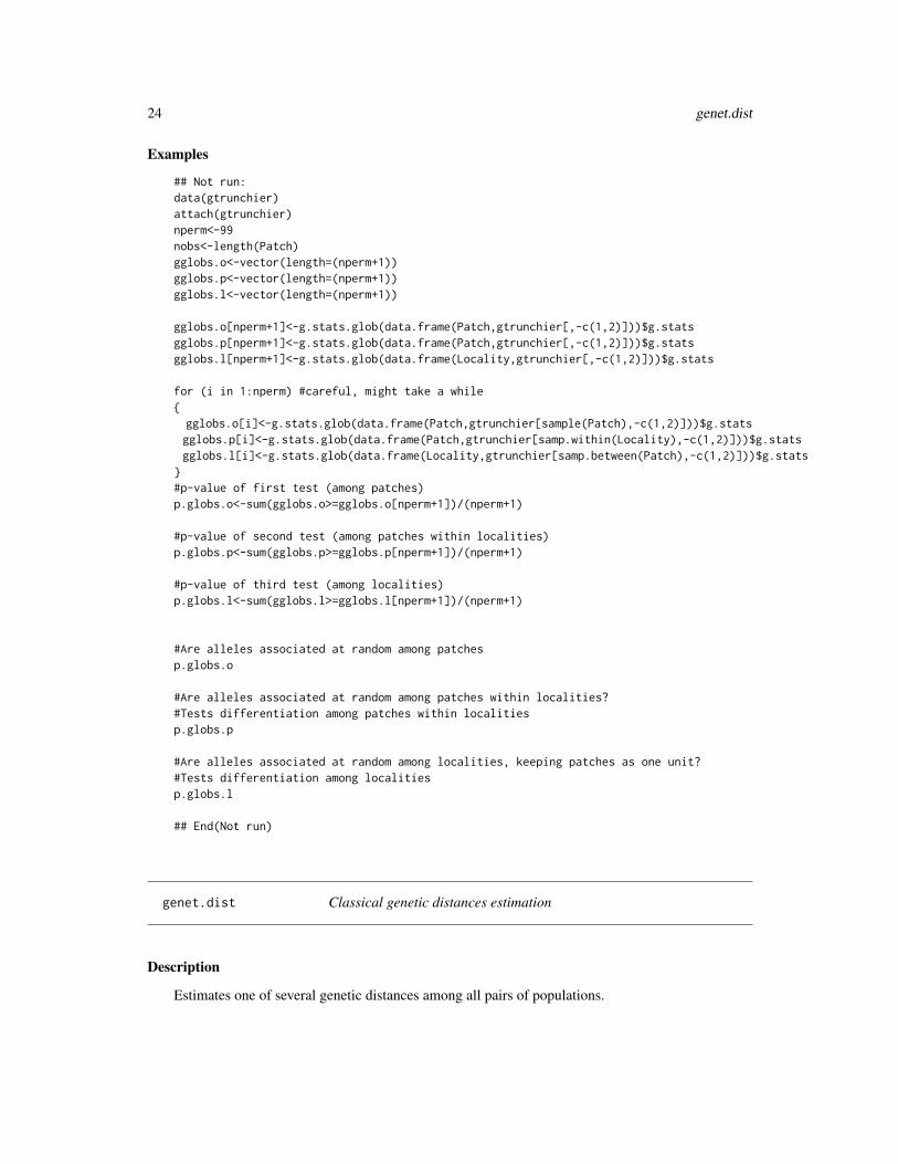
Examples

## Not run:data(gtrunchier)attach(gtrunchier)nperm<-99nobs<-length(Patch)gglobs.o<-vector(length=(nperm+1))gglobs.p<-vector(length=(nperm+1))gglobs.l<-vector(length=(nperm+1))

gglobs.o[nperm+1]<-g.stats.glob(data.frame(Patch,gtrunchier[,-c(1,2)]))$g.statsgglobs.p[nperm+1]<-g.stats.glob(data.frame(Patch,gtrunchier[,-c(1,2)]))$g.statsgglobs.l[nperm+1]<-g.stats.glob(data.frame(Locality,gtrunchier[,-c(1,2)]))$g.stats

for (i in 1:nperm) #careful, might take a while{gglobs.o[i]<-g.stats.glob(data.frame(Patch,gtrunchier[sample(Patch),-c(1,2)]))$g.statsgglobs.p[i]<-g.stats.glob(data.frame(Patch,gtrunchier[samp.within(Locality),-c(1,2)]))$g.statsgglobs.l[i]<-g.stats.glob(data.frame(Locality,gtrunchier[samp.between(Patch),-c(1,2)]))$g.stats

}#p-value of first test (among patches)p.globs.o<-sum(gglobs.o>=gglobs.o[nperm+1])/(nperm+1)

#p-value of second test (among patches within localities)p.globs.p<-sum(gglobs.p>=gglobs.p[nperm+1])/(nperm+1)

#p-value of third test (among localities)p.globs.l<-sum(gglobs.l>=gglobs.l[nperm+1])/(nperm+1)

#Are alleles associated at random among patchesp.globs.o

#Are alleles associated at random among patches within localities?#Tests differentiation among patches within localitiesp.globs.p

#Are alleles associated at random among localities, keeping patches as one unit?#Tests differentiation among localitiesp.globs.l

## End(Not run)

genet.dist Classical genetic distances estimation

Description

Estimates one of several genetic distances among all pairs of populations.

genet.dist 25

Usage

genet.dist(dat,diploid=TRUE,method="Dch")

Arguments


diploid whether the data is from a diploid (default) or haploid organism.method One of “Dch”,“Da”,“Ds”,“Fst”,“Dm”,“Dr”,“Cp” or “X2”, all described in Takezaki

and Nei (1996). Additionally “Nei87” and “WC84” return pairwise FSTs es-timated following Nei (1987) pairwise.neifst and Weir & Cockerham (1984)pp.fst respectively

Details

the method argument specify which genetic distance to use, among eight, all briefly described inTakezaki and Nei (1996)

“Dch” By default, Cavalli-Sforza and Edwards Chord distance (eqn 6 in the reference) is returned.This distance is used as default since Takezaki & Nei (1996) found that it was the best to retrievethe relation among samples.

“Da” This is Nei’s et al genetic distance (eqn 7), performing nearly as well as “Dch”

“Ds” Nei’s standard genetic distance (eqn 1). Increases linearly with diverence time but has largervariance

“Fst” Latter’s and also approximately Reynolds et al Genetic distance (eqn 3)

“Dm” Nei’s minimum distance (eqn 2)

“Dr” Rogers’s distance (eqn 4)

“Cp” Prevosti et al’s distance (eqn 5)

“X2” Sanghvi’s distance (eqn 8)

“Nei87” see pairwise.neifst

“WC84” see pairwise.WCfst

Value

A matrix of pairwise genetic distance

Author(s)


References

Takezaki & Nei (1996) Genetic distances and reconstruction of Phylogenetic trees from microsatel-lite DNA. Genetics 144:389-399

Nei, M. (1987) Molecular Evolutionary Genetics. Columbia University Press

Weir B.S. and Cockerham C.C. (1984) Estimating F-Statistics for the Analysis of Population Struc-ture. Evolution 38:1358


https://onlinelibrary.wiley.com/doi/10.1111/j.1558-5646.1984.tb05657.x

26 genind2hierfstat

See Also

pairwise.WCfst pairwise.neifst

Examples

data(gtrunchier)genet.dist(gtrunchier[,-1])genet.dist(gtrunchier[,-1],method="Dr")

genind2hierfstat Converts genind objects from adegenet into a hierfstat data frame

Description

Converts genind objects from adegenet into a hierfstat data frame

Usage

genind2hierfstat(dat,pop=NULL)

Arguments

dat a genind object

pop a vector containing the population to which each individual belongs. If pop=NULL,pop taken from slot pop of the genind object

Value

a data frame with nloci+1 columns and ninds rows. The first column contains the population iden-tifier, the following the genotypes at each locus

Examples

## Not run:library(adegenet)data(nancycats)genind2hierfstat(nancycats)basic.stats(nancycats)genet.dist(nancycats)data(H3N2)basic.stats(genind2hierfstat(H3N2,pop=rep(1,dim(H3N2@tab)[1])),diploid=FALSE)

## End(Not run)

genot2al 27

genot2al Separates diploid genotypes in its constituant alleles

Description

Separates the input vector of diploid genotypes in two vectors each containing one allele, and returnsa vector of length 2*length(y) with the second part being the second allele

Usage

genot2al(y)

Arguments

y the diploid genotypes at one locus

Value

returns a vector of length 2*length(y), with the second half of the vector containing the secondalleles

Author(s)


<[email protected]>

References

Goudet J. (2004). A library for R to compute and test variance components and F-statistics. In Prep

See Also

varcomp.

Examples

data(gtrunchier)genot2al(gtrunchier[,4])

28 getal.b

getal Converts diploid genotypic data into allelic data

Description

Converts diploid genotypic data into allelic data

Usage

getal(data)

Arguments

data a data frame where the first column contains the population to which the differ-ent individuals belong, and the following columns contain the genotype of theindividuals -one locus per column-

Value

data.al a new data frame, with twice as many row as the input data frame and one extracolumn. each row of the first half of the data frame contains the first allelefor each locus, and each row of the second half of the data frame contains thesecond allel at the locus. The extra column in second position corresponds tothe identifier of the individual to which the allele belongs

Author(s)


Examples

data(gtrunchier)getal(data.frame(gtrunchier[,-2]))

getal.b Converts diploid genotypic data into allelic data

Description

Converts a data frame of genotypic diploid data with as many lines as individuals (ni) and as manycolumns as loci (nl) into an array [ni,nl,2] of allelic data

Usage

getal.b(data)

grm2kinship 29

Arguments

data a data frame with ni rows and nl columns. Each line encodes one individual,each column contains the genotype at one locus of the individual

Value

an array [ni,nl,2] of alleles. The two alleles are stored in the third dimension ofthe array

Author(s)


Examples

data(gtrunchier)#multilocus diploid genotype of the first individualgtrunchier[1,-c(1:2)]#the diploid genotype splitted in its two constituent allelesgetal.b(gtrunchier[,-c(1:2)])[1,,]

grm2kinship Converts a Genetic Relationship Matrix (GRM) to a kinship matrix

Description

Converts a Genetic Relationship Matrix (GRM) to a kinship matrix

Usage

grm2kinship(x)

Arguments

x a square (GRM) matrix

Details

k[ii] = x[ii]− 1; k[ij] = x[ij]/2

Value

a kinship matrix

Author(s)


30 gtrunchier

gtrunchier Genotypes at 6 microsatellite loci of Galba truncatula from differentpatches in Western Switzerland

Description

Data set consisting of the microsatellite genotypes of 370 Galba truncatula, a tiny freshwater snail,collecting from different localities and several patches within localities in Western Switzerland.

Usage

data(gtrunchier)

Value

Locality Identifier of the locality of origin

Patch Identifier of the patch of origin

L21.V Genotype at locus L21.V. For instance the first individual carries allele 2 and 2at this locus

gtrunchier\$L21.V[1]

L37.J Genotype at locus L37.J

L20.B Genotype at locus L20.B

L29.V Genotype at locus L29.V

L36.B Genotype at locus L36.B

L16.J Genotype at locus L16.J

References

Trouve S., L. Degen et al. (2000) Microsatellites in the hermaphroditic snail, Lymnaea truncatula,intermediate host of the liver fluke, Fasciola hepatica.Molecular Ecology 9: 1662-1664.

Trouve S., Degen L. and Goudet J. (2005) Ecological components and evolution of selfing in thefreshwater snail Galba truncatula. Journal of Evolutionary Biology. 18, 358-370

hierfstat 31

hierfstat General information on the hierfstat package

Description

This package contains functions to estimate hierarchical F-statistics for any number of hierarchicallevels using the method described in Yang (1998). It also contains functions allowing to test thesignificance of population differentiation at any given level using the likelihood ratio G-statistic,showed previoulsly to be the most powerful statistic to test for differnetiation (Goudet et al., 1996). The difficulty in a hierarchical design is to identify which units should be permutted. Functionssamp.within and samp.between give permutations of a sequence that allows reordering of theobservations in the original data frame. An exemple of application is given in the help page forfunction g.stats.glob.

Hierfstat includes now all the capabilities of Fstat, and many others. A new serie of functions imple-menting the statistics described in Weir and Goudet (2017) and Goudet et al. (2018) (beta.dosage,fs.dosage) have been written to deal with large genomic data sets and take as input a matrix ofallelic dosages, the number of alternate alleles an individual carries at a locus.

Several functions have been written to simulate genetic data, or to import them from existingsofwares such as quantiNemo or Hudson’s ms

Hierfstat links easily with the gaston, SNPRelate and adegenet packages, among others.

Author(s)


References

Goudet J. (2005) Hierfstat, a package for R to compute and test variance components and F-statistics. Molecular Ecology Notes. 5:184-186


Weir B.S. and Goudet J. (2017) A Unified Characterization of Population Structure and Relatedness.Genetics. 206: 2085-2103

Goudet J., Kay T. and Weir B.S. (2018) How to estimate kinship. Molecular Ecology. 27: 4121:4135


Yang, R.C. (1998) Estimating hierarchical F-statistics. Evolution 52(4):950-956

https://www2.unil.ch/popgen/research/reprints/goudet_men_2005.pdf

https://www.ncbi.nlm.nih.gov/pmc/articles/PMC1207740/pdf/ge14441933.pdf


https://onlinelibrary.wiley.com/doi/full/10.1111/mec.14833

https://onlinelibrary.wiley.com/doi/abs/10.1111/j.1558-5646.1998.tb01824.x

32 indpca

ind.count individual counts

Description

Counts the number of individual genotyped per locus and population

Usage

ind.count(data)

Arguments

data a data frame containing the population of origin in the first column and thegenotypes in the following ones

Value

A table –with np (number of populations) columns and nl (number of loci) rows–of genotype counts

Author(s)


Examples

data(gtrunchier)ind.count(gtrunchier[,-2])

indpca PCA on a matrix of individuals genotypes frequencies

Description

Carry out a PCA on the centered, unscaled matrix of individual’s allele frequencies.

Usage

indpca(dat,ind.labels=NULL,scale=FALSE)

## S3 method for class 'indpca'print(x,...)## S3 method for class 'indpca'plot(x,eigen=FALSE,ax1=1,ax2=2,...)

kinship2dist 33

Arguments

dat A data frame with population of origin as first column, and genotypes in follow-ing columns.

ind.labels a vector of labels for the different individuals

scale whether to standardize each column to variance 1 or to leave it as is (default)

x an indpca object

eigen whether to plot in an additional windows screeplot of the inertias for the differentaxes

ax1 which PCA coordinates to plot on the x axis

ax2 which PCA coordinates to plot on the y axis

... further arguments to pass to print or plot

Value

An object of class indpca with components

call The function call

ipca an object of class pca and dudi (see dudi.pca) in package ade4

mati the original non centered matrice of individuals X alleles frequencies

Author(s)


Examples

##not rundata(gtrunchier)x<-indpca(gtrunchier[,-2],ind.labels=gtrunchier[,2])plot(x,col=gtrunchier[,1],cex=0.7)

kinship2dist Converts a kinship matrix to a distance matrix

Description

Converts a kinship matrix to a distance matrix

Usage

kinship2dist(x)

Arguments

x A square matrix containg kinship coefficients

34 kinship2grm

Details

Dii = 0, Dij = 1−(x−min(x))(1−min(x))

Value

A distance matrix

Author(s)


kinship2grm Converts a kinship matrix to a Genetic Relation Matrix (GRM)

Description

Converts a kinship matrix to a Genetic Relation Matrix (GRM)

Usage

kinship2grm(x)

Arguments

x a square matrix containing kinship coefficients

Details

for off-diagonal elements, GRM = 2× xij ; for diagonal elements, GRM = 1 + xii

Value

a GRM matrix

Author(s)


Examples

## Not run:dos<-matrix(sample(0:2,replace=TRUE,size=1000),nrow=10) #dosage matrix for 10 inds at 100 lociks<-beta.dosage(dos) # kinship matrixkinship2grm(ks)

## End(Not run)

kinshipShift 35

kinshipShift Shifts a kinship matrix

Description

Shifts a kinship matrix

Usage

kinshipShift(x,shift=NULL)

Arguments

x a square matrix

shift the amount by which the elements of x should be shifted. if shift==NULL, theaverage of the off-diagonal elements is substracted

Details

The kinship matrix produced by beta.dosage is relative to the average kinship of the set of indi-viduals analysed (1/(n(n− 1)/2)

∑i

∑j>i xij = 0). Another reference point might be useful, for

instance to avoid negative kinship values, one might want to shift the matrix by min(xij), i 6= j.

Value

the shifted kinship matrix x−shift1−shift

Author(s)


mat2vec Creates a vector from a matrix

Description

creates a vector from a matrix

Usage

mat2vec(mat,upper=FALSE)

Arguments

mat a symmetric matrix

upper whether the upper triangular matrix is to be copied to the vector

36 matching

Value

a vector

Examples

{

mat2vec(matrix(1:16,nrow=4))mat2vec(matrix(1:16,nrow=4),upper=TRUE)

}

matching Estimates matching between pairs of individuals

Description

Estimates matching between pairs of individuals (for each locus, gives 1 if the two individuals arehomozygous for the same allele, 0 if they are homozygous for a different allele, and 1/2 if at leastone individual is heterozygous. Matching is the average of these 0, 1/2 and 1s)

Usage

matching(dos)

Arguments

dos A matrix of 0, 1 and 2s with loci (SNPs) in columns and individuals in rows.missing values are allowed

Details

This function is written for dosage data, i.e., how many doses of an allele (0, 1 or 2) an individualcarries. It should be use for bi-allelic markers only (e.g. SNPs), although you might "force" a kmultiallelic locus to k biallelic loci (see fstat2dos).

Value

a matrix of pairwise matching

ms2bed 37

ms2bed Import the output of the ms program in a BED object

Description

Import the output of the ms program into a BED object, as defined in the gaston package

Usage

ms2bed(fname)

Arguments

fname the name of the text file containing ms output

Value

a bed object

ms2dos Import ms output

Description

Import the output of the ms program into suitable format for further manipulation

Usage

ms2dos(fname)

Arguments

fname a text file containing the output of the ms program

Value

alldat a matrix with as many row as (haploid) individuals and as many columns as SNPs

bim a data frame with two components chr contains the chromosome (replicate) id; pos containsthe SNPs posoition on the chromosome

https://cran.r-project.org/package=gaston

38 pairwise.betas

nb.alleles Number of different alleles

Description

Counts the number of different alleles at each locus and population

Usage

nb.alleles(data,diploid=TRUE)

Arguments

data A data frame containing the population of origin in the first column and thegenotypes in the following ones

diploid whether individuals are diploid

Value

A table, –with np (number of populations) columns and nl (number of loci)rows– of the number of different alleles

Author(s)


Examples

data(gtrunchier)nb.alleles(gtrunchier[,-2])

pairwise.betas Estimates pairwise betas according to Weir and Goudet (2017)

Description

Estimates pairwise betas according to Weir and Goudet (2017)

Usage

pairwise.betas(dat,diploid=TRUE)

Arguments



pairwise.neifst 39

Value

a matrix of pairwise betas

Author(s)



Examples

data(gtrunchier)pairwise.betas(gtrunchier[,-2],diploid=TRUE)

pairwise.neifst Estimates pairwise FSTs according to Nei (1987)

Description

Estimate pairwise FSTs according to Nei (1987)

Usage

pairwise.neifst(dat,diploid=TRUE)

Arguments



Details

FST are calculated using Nei (87) equations for FST’, as described in the note section of basic.stats

Value

A matrix of pairwise FSTs

Author(s)


References

Nei, M. (1987) Molecular Evolutionary Genetics. Columbia University Press


40 pairwise.WCfst

See Also

pairwise.WCfst genet.dist basic.stats

Examples

data(gtrunchier)pairwise.neifst(gtrunchier[,-2],diploid=TRUE)

pairwise.WCfst Estimates pairwise FSTs according to Weir and Cockerham (1984)

Description

Estimates pairwise FSTs according to Weir and Cockerham (1984)

Usage

pairwise.WCfst(dat,diploid=TRUE)

Arguments



Details

FST are calculated using Weir & Cockerham (1984) equations for FST’, as described in the notesection of wc

Value

A matrix of pairwise FSTs

Author(s)


References




pcoa 41

See Also

pairwise.neifst genet.dist

Examples

data(gtrunchier)pairwise.WCfst(gtrunchier[,-2],diploid=TRUE)

pcoa Principal coordinate analysis

Description

principal coordinates analysis as described in Legendre & Legendre Numerical Ecology

Usage

pcoa(mat,plotit=TRUE,...)

Arguments

mat a distance matrix

plotit Whether to produce a plot of the pcoa

... further arguments (graphical for instance) to pass to the function

Value

valp the eigen values of the pcoa

vecp the eigen vectors of the pcoa (the coordinates of observations)

eucl The cumulative euclidian distances among observations,

Author(s)


Examples

data(gtrunchier)colo<-c("black","red","blue","yellow","orange","green")pcoa(as.matrix(genet.dist(gtrunchier[,-1])),col=rep(colo,c(5,5,4,5,5,5)))

42 pop.freq

pi.dosage Estimates nucleotide diversity (π) from dosage data

Description

Estimates nucleotide diversity π =∑

l 2pl(1− pl)2n/(2n− 1) from a dosage matrix

Usage

pi.dosage(dos,L=NULL)

Arguments

dos a ni X nl dosage matrix containing the number of derived/alternate alleles eachindividual carries at each SNP

L the length of the sequence

Value

if L=NULL (default), returns the sum over SNPs of nucleotide diversity; otherwise return the averagenucleotide diversity per nucleotide given the length L of the sequence

pop.freq Allelic frequencies

Description

Estimates allelic frequencies for each population and locus

Usage

pop.freq(dat,diploid=TRUE)

Arguments

dat a data frame where the first column contains the population to which the differ-ent individuals belong, and the following columns contain the genotype of theindividuals -one locus per column-

diploid specify whether the data set consists of diploid (default) or haploid data

Value

A list containing allele frequencies. Each element of the list is one locus. Foreach locus, Populations are in columns and alleles in rows

pp.fst 43

Author(s)


Examples

data(gtrunchier)pop.freq(gtrunchier[,-2])

pp.fst fst per pair

Description

fst per pair following Weir and Cockerham (1984)

Usage

pp.fst(dat=dat,diploid=TRUE,...)

Arguments


diploid whether data from diploid organism


Value

call function call

fst.pp pairwise Fsts

vc.per.loc for each pair of population, the variance components per locus

Author(s)


References




44 print.pp.fst

pp.sigma.loc wrapper to return per locus variance components

Description

wrapper to return per locus variance components between pairs of samples x & y

Usage

pp.sigma.loc(x,y,dat=dat,diploid=TRUE,...)

Arguments

x,y samples 1 and 2dat a genetic data setdiploid whether dats are diploid... further arguments to pass to the function

Value

sigma.loc variance components per locus

Author(s)


print.pp.fst print function for pp.fst

Description

print function for pp.fst

Usage

## S3 method for class 'pp.fst'print(x,...)

Arguments

x an object of class pp.fst... further arguments to pass to the function

Author(s)


qn2.read.fstat 45

qn2.read.fstat Read QuantiNemo extended format for genotype files Read Quan-tiNemo (http://www2.unil.ch/popgen/softwares/quantinemo/)genotype files extended format (option 2)

Description

Read QuantiNemo extended format for genotype files

Read QuantiNemo (http://www2.unil.ch/popgen/softwares/quantinemo/) genotype files ex-tended format (option 2)

Usage

qn2.read.fstat(fname, na.s = c("NA","NaN"))

Arguments

fname quantinemo file name

na.s na string used

Value

dat a data frame with nloc+1 columns, the first being the population to which the individual belongsand the next being the genotypes, one column per locus; and ninds rows

sex the sex of the individuals

Author(s)


References

Neuenschwander S, Michaud F, Goudet J (2019) QuantiNemo 2: a Swiss knife to simulate complexdemographic and genetic scenarios, forward and backward in time. Bioinformatics 35:886

Neuenschwander S, Hospital F, Guillaume F, Goudet J (2008) quantiNEMO: an individual-basedprogram to simulate quantitative traits with explicit genetic architecture in a dynamic metapopula-tion. Bioinformatics 24:1552

See Also

read.fstat

Examples

dat<-qn2.read.fstat(system.file("extdata","qn2_sex.dat",package="hierfstat"))sexbias.test(dat[[1]],sex=dat[[2]])

http://www2.unil.ch/popgen/softwares/quantinemo/

http://www2.unil.ch/popgen/softwares/quantinemo/

https://pubmed.ncbi.nlm.nih.gov/30816926/

https://academic.oup.com/bioinformatics/article/24/13/1552/237901

46 read.fstat

read.fstat Reads data from a FSTAT file

Description

Imports a FSTAT data file into R. The data frame created is made of nl+1 columns, nl being thenumber of loci. The first column corresponds to the Population identifier, the following columnscontains the genotypes of the individuals.

Usage

read.fstat(fname, na.s = c("0","00","000","0000","00000","000000","NA"))

Arguments

fname a file in the FSTAT format (http://www.unil.ch/popgen/softwares/fstat.htm): The file must have the following format:The first line contains 4 numbers: the number of samples, np , the number ofloci, nl, the highest number used to label an allele, nu, and a 1 if the code foralleles is a one digit number (1-9), a 2 if code for alleles is a 2 digit number(01-99) or a 3 if code for alleles is a 3 digit number (001-999). These 4 numbersneed to be separated by any number of spaces.The first line is immediately followed by nl lines, each containing the name ofa locus, in the order they will appear in the rest of the file.On line nl+2, a series of numbers as follow:

1 0102 0103 0101 0203 0 0303

The first number identifies the sample to which the individual belongs, the sec-ond is the genotype of the individual at the first locus, coded with a 2 digitsnumber for each allele, the third is the genotype at the second locus, until locusnl is entered (in the example above, nl=6). Missing genotypes are encoded with0, 00, 0000, 000000 or NA. Note that 0001 or 0100 are not a valid format, asboth alleles at a locus have to be known, otherwise, the genotype is consideredas missing. No empty lines are needed between samples.

na.s The strings that correspond to the missing value. You should note have to changethis

Value

a data frame containing the desired data, in a format adequate to pass to varcomp

References

Goudet J. (1995). FSTAT (Version 1.2): A computer program to calculate F- statistics. Journal ofHeredity 86:485-486


http://www.unil.ch/popgen/softwares/fstat.htm


read.fstat.data 47

Examples

read.fstat(paste(path.package("hierfstat"),"/extdata/diploid.dat",sep="",collapse=""))

read.fstat.data Reads data from a FSTAT file

Description

Imports a FSTAT data file into R. The data frame created is made of nl+1 columns, nl being thenumber of loci. The first column corresponds to the Population identifier, the following columnscontains the genotypes of the individuals.

Usage

read.fstat.data(fname, na.s = c("0","00","000","0000","00000","000000","NA"))

Arguments

fname a file in the FSTAT format (http://www.unil.ch/popgen/softwares/fstat.htm): The file must have the following format:The first line contains 4 numbers: the number of samples, np , the number ofloci, nl, the highest number used to label an allele, nu, and a 1 if the code foralleles is a one digit number (1-9), a 2 if code for alleles is a 2 digit number(01-99) or a 3 if code for alleles is a 3 digit number (001-999). These 4 numbersneed to be separated by any number of spaces.The first line is immediately followed by nl lines, each containing the name ofa locus, in the order they will appear in the rest of the file.On line nl+2, a series of numbers as follow:

1 0102 0103 0101 0203 0 0303

The first number identifies the sample to which the individual belongs, the sec-ond is the genotype of the individual at the first locus, coded with a 2 digitsnumber for each allele, the third is the genotype at the second locus, until locusnl is entered (in the example above, nl=6). Missing genotypes are encoded with0, 00, 0000, 000000 or NA. Note that 0001 or 0100 are not a valid format, asboth alleles at a locus have to be known, otherwise, the genotype is consideredas missing. No empty lines are needed between samples.

na.s The strings that correspond to the missing value. You should note have to changethis

Value

a data frame containing the desired data, in a format adequate to pass to varcomp



48 read.ms

References



Examples

read.fstat.data(paste(path.package("hierfstat"),"/extdata/diploid.dat",sep="",collapse=""))

read.ms Read data generated by Hudson ms program Read data generated byRhrefhttp://home.uchicago.edu/rhudson1/source/mksamples.htmlHudsonms program, either as Haplotypes or as SNPs.

Description

With argument what="SNP", each site is read as a SNP, with the ancestral allele encoded as 0 and thealternate allele encoded as 1. If the ms output file contains several replicates, the different replicateswill be collated together. Hence, the number of loci is the sum of all sites from all replicates.

Usage

read.ms(fname,what=c("SNP","Haplotype"))

Arguments

fname file name containing ms output

what whether to read ms output as SNPs or haplotypes

Details

With argument what="Haplotype", each different sequence from a replicate is read as a haplotype,by converting it first to a factor, and then to an integer. There will be as many loci as there arereplicates, and the number of alleles per locus will be the number of different haplotypes in thecorresponding replicate.

Value

alldat a data frame with nloc+1 columns, the first being the population to which the individual be-longs and the next being the genotypes, one column per locus; and one row per (haploid) individual.

Author(s)


read.VCF 49

References

Hudson, R. R. (2002) Generating samples under a Wright-Fisher neutral model of genetic variation.Bioinformatics 18 : 337-338.

Examples

## Not run:datH<-read.ms(system.file("extdata","2pops_asspop.txt",package="hierfstat"),what="Haplotype")dim(datH)head(datH[,1:10]datS<-read.ms(system.file("extdata","2pops_asspop.txt",package="hierfstat"),what="SNP")dim(datS)head(datS[,1:10])

## End(Not run)

read.VCF Reads a VCF file into a BED object

Description

Reads a https://samtools.github.io/hts-specs/Variant Call Format (VCF) file into a BEDobject, retaining bi-allelic SNPs only

Usage

read.VCF(fname,BiAllelic=TRUE,...)

Arguments

fname VCF file name. The VCF file can be compressed (VCF.gz)BiAllelic Logical. If TRUE, only bi-allelic SNPs are retained, otherwise, all variant are

kept... other arguments to pass to the function

Value

A bed.matrix-class object

See Also

read.vcf

Examples

filepath <-system.file("extdata", "LCT.vcf.gz", package="gaston")x1 <- read.VCF( filepath )x1

https://academic.oup.com/bioinformatics/article-abstract/18/2/337/225783

https://samtools.github.io/hts-specs/

50 samp.between

samp.between Shuffles a sequence among groups defined by the input vector

Description

Used to generate a permutation of a sequence 1:length(lev). blocks of observations are permut-ted, according to the vector lev passed to the function.

Usage

samp.between(lev)

Arguments

lev a vector containing the groups to be permuted.

Value

a vector 1:length(lev) (with blocks defined by data) randomly permuted. Usually, one passes theresult to reorder observations in a data set in order to carry out permutation-based tests

Author(s)


<[email protected]>

References


See Also

samp.within, g.stats.glob.

Examples

samp.between(rep(1:4,each=4))#for an application see example in g.stats.glob

samp.between.within 51

samp.between.within Shuffles a sequence

Description

Used to generate a permutation of a sequence 1:length(inner.lev). blocks of observations de-fined by inner.lev are permutted within blocks defined by outer.lev

Usage

samp.between.within(inner.lev, outer.lev)

Arguments

inner.lev a vector containing the groups to be permuted.

outer.lev a vector containing teh blocks within which observations are to be kept.

Value

a vector 1:length(lev) (with blocks defined by data) randomly permuted. Usually, one passes theresult to reorder observations in a data set in order to carry out permutation-based tests

See Also

test.between.within.

samp.within Shuffles a sequence within groups defined by the input vector

Description

Used to generate a permutation of a sequence 1:length(lev). observations are permutted withinblocks, according to the vector lev passed to the function.

Usage

samp.within(lev)

Arguments

lev a vector containing the group to which belongs the observations to be permuted.

52 sexbias.test

Value

a vector 1:length(lev) (with blocks defined by

lev

) randomly permuted. Usually, one passes the result to reorder observations in a data set in order tocarry out permutation-based tests.

Author(s)


<[email protected]>

References


See Also

samp.between,g.stats.glob.

Examples

samp.within(rep(1:4,each=4))#for an application see example in g.stats.glob

sexbias.test Test for sex biased dispersal

Description

Test whether one sex disperses more than the other using the method described in Goudet etal.(2002)

Usage

sexbias.test(dat,sex,nperm=NULL,test="mAIc",alternative="two.sided")

Arguments

dat a data frame with n.locs+1 columns and n.inds rows

sex a vector containing the individual’s sex

nperm the number of permutation to carry out

test one of "mAIc" (default), "vAIc","FIS" or "FST"

alternative one of "two.sided" (default),"less" or "greater"



sim.freq 53

Value

call the function call

res the observation for each sex

statistic the observed statistic for the chosen test

p.value the p-value of the hypothesis

Author(s)


References


Examples

data(crocrussula)sexbias.test(crocrussula$genot,crocrussula$sex)dat<-qn2.read.fstat(system.file("extdata","qn2_sex.dat",package="hierfstat"))sexbias.test(dat[[1]],sex=dat[[2]])## Not run:sexbias.test(crocrussula$genot,crocrussula$sex,nperm=1000)sexbias.test(dat[[1]],sex=dat[[2]],nperm=100,test="FST",alternative="greater")

## End(Not run)

sim.freq Simulates frequencies, for internal use only

Description

Simulates frequencies, for internal use only

sim.genot Simulates genotypes in an island model at equilibrium

Description

Simulates genotypes from several individuals in several populations at several loci in an islandmodel at equilibrium. The islands may differ in size and inbreeding coeeficients.

Usage

sim.genot(size=50,nbal=4,nbloc=5,nbpop=3,N=1000,mig=0.001,mut=0.0001,f=0)


54 sim.genot.metapop.t

Arguments

size The number of individuals to sample per population

nbal The maximum number of alleles present at a locus

nbloc The number of loci to simulate

nbpop The number of populations to simulate

N The population sizes for each island

mig the proportion of migration among islands

mut The loci mutation rate

f the inbreeding coefficient for each island

Value

a data frame with nbpop*size lines and nbloc+1 columns. Individuals are in rows and genotypes incolumns, the first column being the population identifier

Author(s)


Examples

## Not run:dat<-sim.genot(nbpop=4,nbal=20,nbloc=10,mig=0.001,mut=0.0001,N=c(100,100,1000,1000),f=0)betas(dat)$betaiovl

## End(Not run)

sim.genot.metapop.t Simulate genetic data from a metapopulation model

Description

This function allows to simulate genetic data from a metapopulation model, where each popula-tion can have a different size and a different inbreeding coefficient, and migration between eachpopulation is given in a migration matrix.

This function simulates genetic data under a migration matrix model. Each population i sends aproportion of migrant alleles mij to population j and receives a proportion of migrant alleles mji

from population j.

Usage

sim.genot.metapop.t(size=50,nbal=4,nbloc=5,nbpop=3,N=1000,mig=diag(3),mut=0.0001,f=0,t=100)

sim.genot.metapop.t 55

Arguments

size the number of sampled individuals per population

nbal the number of alleles per locus (maximum of 99)

nbloc the number of loci to simulate

nbpop the number of populations to simulate

N the effective population sizes of each population. If only one number, all popu-lations are assumed to be of the same size

mig a matrix with nbpop rows and columns giving the migration rate from populationi (in row) to population j (in column). Each row must sum to 1.

mut the mutation rate of the loci

f the inbreeding coefficient for each population

t the number of generation since the islands were created

Details

In this model, θt can be written as a function of population size Ni, migration rate mij , mutationrate µ and θ(t−1).

The rational is as follows:

With probability 1Ni

, 2 alleles from 2 different individuals in the current generation are sampledfrom the same individual of the previous generation:

-Half the time, the same allele is drawn from the parent;

-The other half, two different alleles are drawn, but they are identical in proportion θ(t−1).

-With probability 1− 1Ni

, the 2 alleles are drawn from different individuals in the previous genera-tion, in which case they are identical in proportion θ(t−1).

This holds providing that neither alleles have mutated or migrated. This is the case with probabilitym2

ii × (1− µ)2. If an allele is a mutant, then its coancestry with another allele is 0.

Note also that the mutation scheme assumed is the infinite allele (or site) model. If the numberof alleles is finite (as will be the case in what follows), the corresponding mutation model is theK-allele model and the mutation rate has to be adjusted to µ′ = K−1

K µ.

Continue derivation

Value

A data frame with size*nbpop rows and nbloc+1 columns. Each row is an individual, the firstcolumn contains the identifier of the population to which the individual belongs, the followingnbloc columns contain the genotype for each locus.

Author(s)


56 sim.genot.t

Examples

#2 populationspsize<-c(10,1000)mig.mat<-matrix(c(0.99,0.01,0.1,0.9),nrow=2,byrow=TRUE)dat<-sim.genot.metapop.t(nbal=10,nbloc=100,nbpop=2,N=psize,mig=mig.mat,mut=0.00001,t=100)betas(dat)$betaiovl # Population specific estimator of FST

#1D stepping stone## Not run:np<-10m<-0.2mig.mat<-diag(np)*(1-m)diag(mig.mat[-1,-np])<-m/2diag(mig.mat[-np,-1])<-m/2mig.mat[1,1:2]<-c(1-m/2,m/2)mig.mat[np,(np-1):np]<-c(m/2,1-m/2)dat<-sim.genot.metapop.t(nbal=10,nbloc=50,nbpop=np,mig=mig.mat,t=400)pcoa(as.matrix(genet.dist(dat))) # principal coordinates plot

## End(Not run)

sim.genot.t Simulate data from a non equilibrium continent-island model

Description

This function allows to simulate genetic data from a non-equilibrium continent-island model, whereeach island can have a different size and a different inbreeding coefficient.

This function simulates genetic data under the continent-islands model (IIM=TRUE) or the finiteisland model (IIM=FALSE). In the IIM, a continent of infinite size sends migrants to islands offinite sizes Ni at a rate m. Alleles can also mutate to a new state at a rate µ. Under this model, theexpected FSTi, θi, can be calculated and compared to empirical estimates.

Usage

sim.genot.t(size=50,nbal=4,nbloc=5,nbpop=3,N=1000,mig=0.001,mut=0.0001,f=0,t=100,IIM=TRUE)

Arguments

size the number of sampled individuals per island

nbal the number of alleles per locus (maximum of 99)

nbloc the number of loci to simulate

nbpop the number of islands to simulate

sim.genot.t 57

N the effective population sizes of each island. If only one number, all islands areassumed to be of the same size

mig the migration rate from the continent to the islands

mut the mutation rate of the loci

f the inbreeding coefficient for each island

t the number of generation since the islands were created

IIM whether to simulate a continent island Model (default) or a migrant pool islandModel

Details

In this model, θt can be written as a function of population size Ni, migration rate m, mutation rateµ and θ(t−1).

The rational is as follows:

With probability 1N , 2 alleles from 2 different individuals in the current generation are sampled

from the same individual of the previous generation:

-Half the time, the same allele is drawn from the parent;

-The other half, two different alleles are drawn, but they are identical in proportion θ(t−1).

-With probability 1− 1N , the 2 alleles are drawn from different individuals in the previous generation,

in which case they are identical in proportion θ(t−1).

This holds providing that neither alleles have mutated or migrated. This is the case with probability(1−m)2 × (1− µ)2. If an allele is a mutant or a migrant, then its coancestry with another allele is0 in the infinite continent-islands model (it is not the case in the finite island model).

Note also that the mutation scheme assumed is the infinite allele (or site) model. If the numberof alleles is finite (as will be the case in what follows), the corresponding mutation model is theK-allele model and the mutation rate has to be adjusted to µ′ = K−1

K µ.

Lets substitute α for (1−m)2(1− µ)2 and x for 12N .

The expectation of FST , θ can be written as:

θt = (α(1− x))tθ0 +x

1− x

t∑i=1

(α(1− x))i

which reduces to θt = x1−x

∑ti=1(α(1− x))i if θ0 = 0.

Transition equations for theta in the migrant-pool island model (IIM=FALSE) are given in Rouseet(1996). Currently, the migrant pool is made of equal contribution from each island, irrespective oftheir size.

Value

A data frame with size*nbpop rows and nbloc+1 columns. Each row is an individual, the firstcolumn contains the island to which the individual belongs, the following nbloc columns containthe genotype for each locus.

58 subsampind

Author(s)


References

Rousset, F. (1996) Equilibrium values of measures of population subdivision for stepwise mutationprocesses. Genetics 142:1357

Examples

psize<-c(100,1000,10000,100000,1000000)dat<-sim.genot.t(nbal=4,nbloc=20,nbpop=5,N=psize,mig=0.001,mut=0.0001,t=100)summary(wc(dat)) #Weir and cockerham overall estimators of FST & FISbetas(dat) # Population specific estimator of FST

subsampind Subsample a FSTAT data frame

Description

Subsample a given number of individuals from a FSTAT data frame

Usage

subsampind(dat,sampsize = 10)

Arguments

dat A data frame with population of origin as first column, and genotypes in follow-ing columns.

sampsize the number of individuals to sample in each population.

Value

A data frame with population of origin as first column, and genotypes in following columns. Eachpopulation is made of at most sampsize individuals

Author(s)


Examples

data(gtrunchier)subsampind(gtrunchier[,-1],6) # check the warning

https://pubmed.ncbi.nlm.nih.gov/8846911/

TajimaD.dosage 59

TajimaD.dosage Estimates Tajima’s D

Description

Estimates Tajima’s D from dosage data

Usage

TajimaD.dosage(dos)

Arguments


Value

Tajima’s D (eqn 38 of Tajima, 1989)

References

Tajima F. 1989 Statistical Method for Testing the Neutral Mutation Hypothesis by DNA Polymor-phism. Genetics 123:585-595.

test.between Tests the significance of the effect of test.lev on genetic differentiation

Description

Tests the significance of the effect of test.lev on genetic differentiation

Usage

test.between(data, test.lev, rand.unit, nperm, ...)

Arguments

data a data frame containing the genotypes for the different loci

test.lev A vector containing the units from which to construct the contingency tables

rand.unit A vector containing the assignment of each observation to the units to be per-mutted

nperm The number of permutations to carry out for the test

... Mainly here to allow passing diploid=FALSE if necessary

https://www.ncbi.nlm.nih.gov/pmc/articles/PMC1203831/

60 test.between.within

Value

g.star A vector containing all the generated g-statistics, the last one beeing the ob-served

p.val The p-value associated with the test

Author(s)


Examples

data(gtrunchier)attach(gtrunchier)#test whether the locality level has a significant effect on genetic structuringtest.between(gtrunchier[,-c(1,2)],test.lev=Locality,rand.unit=Patch)

test.between.within Tests the significance of the effect of test.lev on genetic differentiation

Description

Tests, using permutations of rand.unit within units defined by the vector within the significanceof the contingency tables allele X (levels of test.lev)

Usage

test.between.within(data, within, test.lev, rand.unit, nperm, ...)

Arguments


within A vector containing the units in which to keep the observations


rand.unit A vector containing the assignment of each observation to the units to be per-mutted



Value



test.g 61

Author(s)


Examples

data(yangex)attach(yangex)#tests for the effect of spop on genetic structuretest.between.within(data.frame(genot),within=pop,test=spop,rand=sspop)

test.g Tests the significance of the effect of level on genetic differentiation

Description

Tests the significance of the effect of level on genetic differentiation

Usage

test.g(data = data, level, nperm = 100,...)

Arguments


level A vector containing the assignment of each observation to its level



Value



Author(s)


Examples

data(gtrunchier)attach(gtrunchier)test.g(gtrunchier[,-c(1,2)],Locality)

62 test.within

test.within Tests the significance of the effect of inner.level on genetic differentia-tion within blocks defined by outer.level

Description

Tests the significance of the effect of inner.level on genetic differentiation within blocks defined byouter.level

Usage

test.within(data, within, test.lev, nperm, ...)

Arguments


within A vector containing the units in which to keep the observations




Value



Author(s)


Examples

data(gtrunchier)attach(gtrunchier)#tests whether the patch level has a significant effect on genetic structuretest.within(gtrunchier[,-c(1,2)],within=Locality,test.lev=Patch)

theta.Watt.dosage 63

theta.Watt.dosage Estimates θ_Watterson from dosage data

Description

Estimates θWatterson = S/a, where S is the number of segregating sites in a set of sequences anda = 1/

∑n−1i i.

Usage

theta.Watt.dosage(dos,L=NULL)

Arguments


L the length of the sequence

Value

if L=NULL (default), returns θWatterson, else return θWatterson/L

varcomp Estimates variance components for each allele of a locus

Description

Estimates variance components for each allele for a (fully) hierarchical random design defined byall but the last column of the data frame data, the last column containing the genetic data to analyse.Columns for the hierarchical design should be given from the outermost to the innermost before theindividual (e.g. continent, region, population, patch,...)

Usage

varcomp(data,diploid=TRUE)

Arguments

data a data frame that contains the different factors from the outermost (e.g. region)to the innermost before the individual. the last column of the data frame ’data’contains the locus to analyse, which can be multiallelic. Missing data are al-lowed.

diploid a boolean stating whether the data come from diploid (TRUE=default) or hap-loid (FALSE) organisms

64 varcomp

Details

The format for genotypes is simply the code for the 2 alleles put one behind the other, without spacein between. For instance if allele 1 at the locus has code 23 and allele 2 39, the genotype format is2339.

Value

df the degrees of freedom for each level

k the k matrix, the coefficients associated with the variance components

res the variance components for each allele

overall the variance components summed over alleles

F a matrix of hierarchical F-statistics type-coefficients with the first line corre-sponding toF(n−1)/n,F(n−2)/n...Fi/n and the diagonal corresponding toF(n−1)/n,F(n−2)/(n−1),Fi/2

Author(s)


<[email protected]>

http://www.unil.ch/popgen/people/jerome.htm

References



Yang, R.C. (1998). Estimating hierarchical F-statistics. Evolution 52(4):950-956

See Also

varcomp.glob.

Examples

#load data setdata(gtrunchier)attach(gtrunchier)#varcomp(data.frame(Locality,Patch,L21.V))

http://www.unil.ch/popgen/people/jerome.htm

varcomp.glob 65

varcomp.glob Estimate variance components and hierarchical F-statistics over allloci

Description

Return multilocus estimators of variance components and F-statistics

Usage

varcomp.glob(levels=levels,loci=loci,diploid=TRUE)

Arguments

levels a data frame containing the different levels (factors) from the outermost (e.g.region) to the innermost before the individual

loci a data frame containing the different loci

diploid Specify whether the data are coming from diploid or haploid organisms (diploidis the default)

Value

loc The variance components for each locus

overall The variance components summed over all loci

F a matrix of hierarchical F-statistics type-coefficients with the first line corre-sponding toF(n−1)/n,F(n−2)/n...Fi/n and the diagonal corresponding toF(n−1)/n,F(n−2)/(n−1),Fi/2

Author(s)

Jerome Goudet DEE, UNIL, CH-1015 Lausanne Switzerland

<[email protected]>

References




See Also

varcomp.

66 vec2mat

Examples

#load data setdata(gtrunchier)attach(gtrunchier)varcomp.glob(data.frame(Locality,Patch),gtrunchier[,-c(1,2)])

vec2mat Fills a triangular matrix from the inputed vector

Description

Fills a triangular matrix from the inputed vector

Usage

vec2mat(x,diag=FALSE,upper=FALSE)

Arguments

x a vector

diag whether the vector contains the diagonal elements

upper whether the vector contains the upper trinagular matrix elements

Value

a matrix

Examples

{vec2mat(1:10)vec2mat(1:10,diag=TRUE)vec2mat(1:10,upper=TRUE)

}

wc 67

wc Computes Weir and Cockrham estimates of Fstatistics

Description

Computes Weir and Cockerham estimates of Fstatistics

Usage

wc(ndat,diploid=TRUE,pol=0.0)

## S3 method for class 'wc'print(x,...)

Arguments

ndat data frame with first column indicating population of origin and following rep-resenting loci

diploid Whether data are diploid

pol level of polymorphism reqesuted for inclusion. Note used for now

x an object of class wc

... further arguments to pass to print.wc

Value

sigma variance components of allele frequencies for each allele, in the order amongpopulations, among individuals within populations and within individuals

sigma.loc variance components per locus

per.al FST and FIS per allele

per.loc FST and FIS per locus

FST FST overall loci

FIS FIS overall loci

Author(s)


Examples

data(gtrunchier)wc(gtrunchier[,-1])

68 write.fstat

write.bayescan Writes a bayescan file

Description

write the genotypes in a format suitable for analysis with bayescan

Usage

write.bayescan(dat=dat,diploid=TRUE,fn="dat.bsc")

Arguments

dat a genotype data frame

diploid whether the dataset is diploid or haploid

fn file name for output

Value

a text file fn is written in the current directory

Author(s)


References

Foll M and OE Gaggiotti (2008) Genetics 180: 977-993

http://cmpg.unibe.ch/software/BayeScan/

write.fstat Write an Fstat data file

Description

Write a data frame to a text file in the fstat data format, see read.fstat

Usage

write.fstat(dat,fname="genotypes.dat")

Arguments

dat A data frame with first column containing the population identifier and remain-ing columns containing genotypes

fname The name of teh text file to which the data frame should be written

https://www.genetics.org/content/180/2/977.abstract

http://cmpg.unibe.ch/software/BayeScan/

write.ped 69

Value

None

Author(s)

Jerome Goudet

References


Examples

## Not run: data(gtrunchier)write.fstat(gtrunchier[,-1],"galba.dat")

## End(Not run)

write.ped Write ped file for analyses with PLINK

Description

write a ped and a map file suitable for analysis with PLINK

Usage

write.ped(dat, ilab = NULL, pop = NULL,fname = "dat",na.str="0",f.id=NULL,m.id=NULL,loc.pos=NULL,sex=NULL)

Arguments

dat a hierfstat data frame. if pop=NULL, the first column should contain the popu-lation identifier, otherwise it contains genotypes at the first locus

ilab individual labels

pop population id

fname filename for ped file

na.str character string to use for missing values

f.id father id. default to unknown

m.id mother id. default to unknown

loc.pos the loci position default to unknown

sex the individual sex. default to unknown

https://www.cog-genomics.org/plink2

70 write.struct

Value

a map file containing the loci positions

a ped file containing genotypes etc...

References

Chang et al. (2015) Second-generation PLINK: rising to the challenge of larger and richer datasets

write.struct Write structure file

Description

Write a genotype data set to a file in the structure format

Usage

write.struct(dat,ilab=NULL,pop=NULL,MARKERNAMES=FALSE,MISSING=-9,fname="dat.str")

Arguments

dat a genotype dataframe

ilab an (optional) column with individual labels

pop an (optional) column with population identifiers

MARKERNAMES whether to add a row with marker names. If TRUE, takes the loci names fromdat

MISSING The code for missing alleles

fname a string containing the file name (default to "dat.str")

Value

a text file in the structure format

Author(s)


References

Pritchard JK etal. 2000. Inference of population structure using multilocus genotype data. Genetics155:945-959

https://academic.oup.com/gigascience/article/4/1/s13742-015-0047-8/2707533

yangex 71

yangex Example data set from Yang (1998) appendix

Description

Reproduce the example data set used in Yang’s paper appendix. The genotype (column genot) isinvented

Usage

data(exhier)

Value

pop outermost level

spop sub pop level

sspop sub sub pop level

genot dummy diploid genotype

References


Examples

data(yangex)varcomp(yangex)#the k matrix should be the same as matrix (A2) in Yang's appendix, p. 956

Index

∗ IOwrite.fstat, 68

∗ datasetscont.isl, 16cont.isl99, 17crocrussula, 17diploid, 18exhier, 19gtrunchier, 30yangex, 71

∗ distancegenet.dist, 24

∗ manipgenot2al, 27getal, 28getal.b, 28read.fstat, 46read.fstat.data, 47samp.between, 50samp.between.within, 51samp.within, 51

∗ miscellaneouswrite.struct, 70

∗ mischierfstat, 31

∗ multivariateindpca, 32

∗ nonparametrictest.between, 59test.between.within, 60test.g, 61test.within, 62

∗ univarallele.count, 4allelic.richness, 5basic.stats, 6boot.ppfis, 13boot.vc, 15g.stats, 22

g.stats.glob, 23ind.count, 32nb.alleles, 38pop.freq, 42pp.fst, 43pp.sigma.loc, 44print.pp.fst, 44varcomp, 63varcomp.glob, 65wc, 67

∗ utilitiessubsampind, 58

AIc, 3allele.count, 4allelic.richness, 5

basic.stats, 6, 39, 40beta.dosage, 8, 11betas, 9, 12, 20biall2dos, 11boot.ppbetas, 12boot.ppfis, 13boot.ppfst, 14boot.vc, 15

cont.isl, 16cont.isl99, 17crocrussula, 17

diploid, 18

exhier, 19

fis.dosage (fs.dosage), 19fs.dosage, 11, 19fst.dosage (fs.dosage), 19fstat2dos, 8, 21, 36

g.stats, 22, 23g.stats.glob, 22, 23, 50, 52

72

INDEX 73

genet.dist, 24, 40, 41genind2hierfstat, 26genot2al, 27getal, 28getal.b, 28grm2kinship, 29gtrunchier, 30

hierfstat, 31Ho (basic.stats), 6Hs (basic.stats), 6

ind.count, 8, 32indpca, 32

kinship2dist, 33kinship2grm, 34kinshipShift, 35

mat2vec, 35matching, 8, 36ms2bed, 37ms2dos, 37

nb.alleles, 38

pairwise.betas, 12, 38pairwise.fst.dosage (fs.dosage), 19pairwise.neifst, 25, 26, 39, 41pairwise.WCfst, 25, 26, 40, 40pcoa, 41pi.dosage, 42plot.fs.dosage (fs.dosage), 19plot.indpca (indpca), 32pop.freq, 8, 42pp.fst, 25, 43pp.sigma.loc, 44print.basic.stats (basic.stats), 6print.betas (betas), 9print.boot.ppfst (boot.ppfst), 14print.fs.dosage (fs.dosage), 19print.indpca (indpca), 32print.pp.fst, 44print.wc (wc), 67

qn2.read.fstat, 45

read.fstat, 45, 46read.fstat.data, 47read.ms, 48

read.VCF, 49read.vcf, 49

samp.between, 23, 50, 52samp.between.within, 51samp.within, 23, 50, 51sexbias.test, 52sim.freq, 53sim.genot, 53sim.genot.metapop.t, 54sim.genot.t, 56subsampind, 58

TajimaD.dosage, 59test.between, 59test.between.within, 51, 60test.g, 61test.within, 62theta.Watt.dosage, 63

varcomp, 27, 63, 65varcomp.glob, 15, 64, 65vec2mat, 66

wc, 40, 67write.bayescan, 68write.fstat, 68write.ped, 69write.struct, 70

yangex, 71

hierfstat: estimation and tests of hierarchical f-statistics

Documents