hierarchical models for estimating state and …gelman/research/published/a12052_shirley.pdf ·...

© 2014 Royal Statistical Society 0964–1998/15/178000

J. R. Statist. Soc. A (2015)

Hierarchical models for estimating state anddemographic trends in US death penalty publicopinion

Kenneth E. Shirley

New York, USA

and Andrew Gelman

Columbia University, New York, USA

[Received August 2012. Final revision October 2013]

Summary.One of the longest running questions that has been regularly included in US nationalpublic opinion polls is ‘Are you in favor of the death penalty for persons convicted of murder?’.Because the death penalty is governed by state laws rather than federal laws, it is of specialinterest to know how public opinion varies by state, and how it has changed over time withineach state. We combine dozens of national polls taken over a 50-year span and fit a Bayesianmultilevel logistic regression model to estimate support for the death penalty as a function ofthe year, the state, state level variables and various individual level demographic variables.Among our findings were that support levels in northeastern and southern states have movedin opposite directions over the past 50 years, support among blacks has decreased relative tonon-blacks, but at slightly different rates for men and women, and support among some edu-cation groups varies widely by region. Throughout the paper, we highlight the use of a varietyof analytical and graphical tools for model understanding, including average predictive com-parisons, finite population contrasts for overparameterized models and graphical summaries ofposterior distributions of group level variance parameters.

Keywords: Gallup survey; General Social Survey; Hierarchical Bayes methods; Markov chainMonte Carlo methods; Multilevel model; Political science

1. Introduction

Capital punishment is perennially popular in the USA but is legal in only about two-thirds ofthe states (and is implemented rarely in many of these). To understand better the relationshipbetween public opinion and policy, it would be desirable to know the support for the deathpenalty in each of the 50 states, and how this support has changed over time. To estimate statelevel effects over time, it is necessary to control for the effects of national swings in publicopinion as well as demographic variables, both of which are known to be large. As Fig. 1illustrates using poll data from the General Social Survey and Gallup polls, national supportfor the death penalty has fluctuated substantially during the past 50 years, beginning withlow support in the 1960s, increasing support throughout the 1970s (when capital punishmentwas ruled unconstitutional by the Supreme Court, followed by new rules under which the deathpenalty reappeared, one state at a time), high support in the 1980s (during which time a national

Address for correspondence: Kenneth E. Shirley, Apartment 6B, 229 West 60th Steet, New York, NY 10023,USA.E-mail: [email protected]

2 K. E. Shirley and A. Gelman

Fig. 1. Proportion of respondents who supported the death penalty by year (j, 95% confidence interval),based on a combination of General Social Survey and Gallup polls: , overall proportion of death penaltysupport across all years (67.5%)

concern about crime made the death penalty a prominent political issue) and, finally, decreasedsupport since the mid-1990s (when five states either explicitly illegalized or indirectly suspendedthe death penalty in part because of the exoneration of numerous death row inmates due to DNAevidence) (Baumgartner et al., 2008). Additionally, studies of individual surveys have repeatedlyshown strong relationships between death penalty support and demographic variables such assex, race, age, education, income and religion, to name just a few (Fox et al., 1991; Ellsworthand Gross, 1994; Hanley, 2008).

Despite the extensive literature on the time series of aggregate death penalty support in theUSA over the past 50 years, and also on individual level predictors of death penalty supportat specific time points (which are reviewed in detail in Section 2), there has been very littlerigorous, simultaneous analysis of both. One of the challenges in modelling demographic, timeseries and state-specific effects simultaneously is that, even after combining multiple surveys, thedata are still too sparse to estimate high level interactions without some form of regularization,or shrinkage towards the mean. Furthermore, the national yearly fluctuations in death penaltysupport do not follow a straightforward pattern that can be embedded in a standard linearmodel. If such a model were fitted to the differences between state-by-state levels of support andtheir average across states, this would be equivalent to treating the national average time seriesas if it were a known quantity, and the result would be the underestimation of the uncertaintyof modelled quantities. Lax and Phillips (2009a) and Franklin (2001) discussed these problemsin the context of public opinion polls and voting behaviour.

Our approach to the problem is to fit a Bayesian multilevel logistic regression model to thedata, where the model is overparameterized to allow for the simultaneous estimation of thenational fluctuations in death penalty support as well as state-by-state deviations from it. Thehierarchical Bayesian approach handles the regularization required for sparse data via priordistributions for groups of parameters and is a common approach for small area estimation(Rao, 2003). The overparameterization of the model is a consequence of modelling yearly

State and Demographic Trends in US Death Penalty Opinion 3

effects by using an auto-regressive AR(1) model, and also modelling state trends aslinear deviations from the national average. We follow Gelfand and Sahu (1999) and useweakly informative priors for the unidentified parameters to speed convergence of the con-trasts of exchangeable parameters within groups, rather than impose constraints to make themodel identifiable.

The model can be fitted by using standard Markov chain Monte Carlo (MCMC) techniques,but assessing convergence, checking the fit of the model and interpreting the parameter estimatesrequire a variety of non-standard tools for understanding complex hierarchical models. Wehighlight our use of these tools throughout our discussion of the fit of the model and theresulting conclusions about death penalty public opinion. First, when we analyse posteriorsamples, we compute finite population contrasts to compare different units within groups, andwe focus our convergence assessments and posterior summaries on these quantities rather thanthe ‘raw’ parameters from the model. Second, we include graphical summaries of the fittedmodel that visualize the variation between respondents within different groups, to discoverwhich categorical predictors explain the most variation in the outcome. The large number ofcategorical predictors and resulting interaction terms in our model make the visual summary ofvariability absolutely necessary for model understanding. Last, we compute average predictivecomparisons to provide an additional high level summary of which predictors explain the mostvariation in death penalty support. This is how we compare, on an equal scale, how much deathpenalty support has changed as a function of time, state residency and demographic variables—a novel comparison that requires the combination of pooling many surveys over time, fitting acomplex model and summarizing the model fit in a succinct way.

We find that public support for the death penalty is highly associated with certain demo-graphic variables, such as sex, race and education, which is consistent with previous research.Our model, however, provides novel estimates of how these effects have changed over time,and how they vary across states, especially with regard to opinion as a function of race andsex. We also find that support for the death penalty has changed significantly within certainstates over time compared with the national average, holding constant the effects of demo-graphic variables. In particular, we find that, before the 1970s, capital punishment was morepopular in the northeast than in the south, which is a surprise given the current pattern inwhich the vast majority of executions are carried out in southern states. Additionally, we findthat some of the variation between state trends can be explained by state level variables in-cluding the legality of the death penalty and shifting partisan support over time, and the restof the variation among states is explained by state-specific effects that we estimate with ourmodel.

The models being developed and evaluated here are relevant not just for death sentencingand criminal justice but also more generally for studying the interactions between state levelopinion and policies, as discussed in literature including Erikson (1976), Datta et al. (1999) andLax and Phillips (2009b). What is important is that the model allows for interactions betweendemographic, geographic and time patterns, so that post-stratification can be done to estimateactual state-by-state levels of support as accurately as possible (which is especially relevant fora public policy that faces a referendum vote).

The rest of the paper is organized as follows: Section 2 reviews previous work on death penaltyopinions, Section 3 contains a description of the data to which we fit the model, Section 4contains a detailed description of the model, Section 5 contains a description of how we com-puted adjusted parameter estimates and post-processed our MCMC output, Section 6 containsa description of the model parameter estimates and other analysis of the fitted model, Sec-tion 7 discusses the goodness of the fit of the model via posterior predictive checks and residual


plots, Section 8 discusses the results of out-of-sample predictions made by the model and similarcompeting models and, last, Section 9 contains a discussion of the results.

2. Public opinion on the death penalty

Opinion on capital punishment has received a large amount of attention in the political scienceliterature for a variety of reasons. First, the death penalty has consistently been an issue ofnational interest since the earliest national opinion polls were conducted by Gallup in the mid-1930s; thus, there is a large amount of historical data concerning death penalty public opinion.Second, there have been multiple Supreme Court decisions concerning death penalty laws thatcite changing public opinion as a factor in determining whether aspects of the death penaltyconstitute ‘cruel and unusual punishment’ (which is forbidden according to the eighth amend-ment in the US Bill of Rights). In Weems versus United States in 1910 and later in Trop versusDulles in 1958, Supreme Court decisions specifically pointed out that the definition of cruel andunusual can change over time according to societal standards (Vidmar and Ellsworth, 1974).Much later, in 2002, Supreme Court Justice John Paul Stevens specifically mentioned that pub-lic opinion polls provided insight concerning the public’s feelings towards the death penalty formentally retarded prisoners (Hanley, 2008). Although individuals rarely exert direct control overdeath penalty laws through state level referendums, these Supreme Court precedents show that,indirectly, death penalty public opinion affects public policy. Various references have exploredthis opinion–policy relationship (Erikson, 1976; Norrander, 2000).

The basic relationships between demographic variables and death penalty support have beenwell understood for decades, but higher level interaction effects have been less studied. Duringthe period in the 1970s when the Supreme Court was shaping modern death penalty policy, Vid-mar and Ellsworth (1974) reviewed then-current public opinion of the death penalty on the basisof a 1972 Gallup poll and previous work by Erskine (1970) tabulating poll results from the late1960s. They found that higher support for the death penalty was associated with respondentswho were male, white, old and less educated. Analyses in the 1990s found similar results (Foxet al., 1991; Ellsworth and Gross, 1994). The question of whether these effects have changed overtime has not been answered rigorously. Baumgartner et al. (2008) suggested that associationsbetween demographic variables and death penalty support are mostly fixed over time, but theydid not fit a quantitative model to back up this claim. Hanley (2008) considered changes insupport as a function of sex and race over time and claimed that, in the 1990s, support amongall race × sex subgroups was higher than it was in the 1970s but did not consider the relativemagnitudes of these differences (in Section 6 we show that, although absolute levels of supportmay have been higher for all groups in the 1990s, the extent to which support among blacks wasbelow the national average was increasing, and at slightly different rates for men and women).Hanley (2008) also pointed out that the relationship between age and support varied duringthe period from 1970 to 2000. Last, they found that the negative correlation between level ofeducation and support is not monotonic; the two least supportive educational groups are thosewithout a high school degree, and those with a graduate degree of some kind (these two groupsoccupy opposite ends of the education scale). Our results in Section 6 are consistent with thisfinding.

The most recent and thorough time series model of death penalty public opinion is found inBaumgartner et al. (2008). They focused on modelling long-term trends in death penalty publicopinion as a function of changing media coverage, using an index of support for the deathpenalty based on a weighted average of yearly changes in support of the death penalty from 292statewide and national surveys between 1953 and 2006 that asked about the death penalty by


using different question wordings. They found a relationship between changes in public opinionand the tone of media coverage and levels of crime. They did not, however, model individualresponses simultaneously as a function of time and demographic variables.

3. The data

We put together data on public opinion of the death penalty in two stages. We started with the21 General Social Survey polls that were given between 1974 and 2000, all of which asked thequestion ‘Do you favor or oppose the death penalty for persons convicted of murder?’. Second,to increase the time span of our observed data, we included data from Gallup polls that weretaken before 1974 and after 2000 that asked a similar question: ‘Are you in favor of the deathpenalty for persons convicted of murder?’. We searched for these Gallup polls in the archiveof the Roper Center for Public Opinion Research and, to our knowledge, we included everyGallup poll in the Roper archive that

(a) asked the question of interest, and(b) was given before 1974 or after 2000, with the exception of the Gallup polls that were given

in 1936 and 1937, which we excluded because they did not include detailed informationabout the level of education of each respondent.

The source of the poll is not a significant factor in the level of support that was expressed byrespondents: Baumgartner et al. (2008) found that the correlation between levels of support fromthe two polling sources, the General Social Survey and Gallup, is 0.90 for the years in which theyboth asked the question of interest, and Schuman and Presser (1981) showed that having formalbalance in a survey question (explicitly suggesting a positive and negative answer in the question)rarely affects the outcome. In all, we modelled data from 34 polls, all of which were taken indistinct years between 1953 and 2006, where the maximum number of years between consecutivepolls was 5 years (between the 1960 and 1965 Gallup polls). The number of respondents perpoll ranged from 445 to 3085, and the total number of responses was N = 58253. We did notweight the responses by using the given survey weights because we include as predictors all thevariables that were used to create the weights, and we compute post-stratified estimates ourselves(see Section 6).

Between 1953 and 2006, the proportion of poll respondents supporting the death penaltyin a given year fluctuated between 47% and 79%, excluding those who had no opinion (theproportion of respondents with no opinion rarely exceeded 10%). Fig. 1 contains a plot ofdeath penalty support by year during this time. In each of the 34 polls we recorded the state ofresidence of each respondent, with the District of Columbia considered as the 51st state. Thenumber of respondents per state per year was highly imbalanced, ranging from an average of0.5 respondents per year in Hawaii (17 responses among the 34 surveys) to 170 respondents peryear in California. We also classified states into four regions—northeast, south, midwest andwest—according to the US census state classification (with the District of Columbia includedin the south). The other information that we used for our models was demographic informationabout each respondent, consisting of the following four variables:

(a) sex (male or female);(b) race (black or non-black);(c) age (a categorical variable with four levels, where level 1 is 18–29 years, level 2 is 30–44

years, level 3 is 45–64 years and level 4 is 65 years or older);(d) education (measured as the highest degree achieved by the respondent, a categorical

variable with five levels, where level 1 is less than high school, level 2 is high school, level 3


is some college or trade school, level 4 is college graduate and level 5 is graduate degree).From this point forward, we call this variable ‘degree’.

Fig. 2 displays some summary statistics of the distributions of each of these four variablesand includes the sample percentage of respondents in each main demographic category whosupported the death penalty.

Last, we considered three state level variables as potential explanatory variables in our model.The first two state level variables are related to the state’s partisan political support, as measuredby their support for Republican versus Democratic presidential candidates throughout the years.Specifically, for each presidential election year from 1952 to 2004, we recorded the Republicanshare of the vote in each state, discarding third-party votes, and then we fitted a linear regressionmodel separately for each state to these percentages by using time as the sole predictor. Werecorded the estimated intercept and slope of this regression model for each state to create twostate level variables per state, which we call the ‘Republican share intercept’ and ‘Republicanshare slope’. We used this simplified predictor instead of using each individual state–time variablebecause presidential election years did not match the years of the surveys.

Third, for each year from 1953 to 2006, we recorded the percentage of years in this 54-yeartime span that the death penalty was legal in each state. There is only a moderate amount ofvariation in this variable across states. The death penalty was legal in 40 states from 1953 to1972 (and in Oregon from 1953 to 1963), and then a Supreme Court decision, Furman versusGeorgia, effectively rendered every state’s death penalty statute illegal in June 1972. About 30states rewrote their death penalty statute during the next 5 years, and seven other states rewrotetheir statutes at some point during the following 20 years. (Iowa, West Virginia and the District

Fig. 2. Exploratory data analysis of the demographic variables (of the four demographic variables recorded,the largest difference in death penalty support exists between blacks and non-blacks; age and education,which are ordinal variables, have non-monotonic relationships with death penalty support): �, proportions ofrespondents in each group who supported the death penalty (pooled across all years and states); —, 95%confidence intervals for the proportions; , overall proportion of death penalty support across all subgroups(about 67.5%)


of Columbia have never rewritten their death penalty statutes since 1972.) In 1976, anotherSupreme Court decision, Gregg versus Georgia, overturned the 1972 ruling and made the deathpenalty legal again. (In both the 1972 decision and the 1976 decision, the Supreme Court ruledon a specific death penalty case, and their ruling set a precedent that was applicable to deathpenalty laws nationwide.) For our definition of this variable, which we call ‘legality’, if a staterewrote their death penalty statute between 1972 and 1976, we include these years as additionalyears in which the death penalty was legal for that state, even though technically every statewas waiting for the court system to rule on the new version of the law during this time, andno executions were attempted. We code the variable this way to measure the degree to whicheach state supported the death penalty legislatively over this period; it is a slightly less precisevariable than the strict percentage of years in which the death penalty was legal, but it increasesthe variation of this state level variable, and it may be associated with public opinion. Acrossall states, the variable legality has a maximum of 1 (Florida rewrote their death penalty law in1972, the same year as the Furman versus Georgia case), and its minimum is 0 (10 states havenever had a death penalty statute during this time span). The mean and standard deviation oflegality are 0.70 and 0.39 respectively.

In summary, there are six categorical variables: year, state, sex, race, age and education. Ageand education are actually ordinal, but we include them as unordered categories in our model.Of the 54×51×2×2×4×5=220320 distinct categories, we have at least one observation fromonly 24103 of them. The high level interaction effects between sets of these categorical variablesrequires a high ratio of parameters to data points, motivating the use of a regression model thatallows for shrinkage, or regularization, such as a multilevel Bayesian model.

4. The model

We fit a series of multilevel models to the data with the main goal of understanding changesin public opinion of the death penalty for different states and demographic groups across time.We began by fitting some exploratory models by using ordinary least squares regression to seewhich main effects and interaction effects were associated with the response, and we used thisprocess to guide which effects to include in the smaller number of multilevel Bayesian modelsthat we fit. We ultimately fit five multilevel Bayesian models of varying complexity to a portionof the data designated for training, and we measured the predictive accuracy of each model (interms of deviance) on a test set. These models, which we shall describe in detail in Section 8,are differentiated by the complexity of the interaction effects that they included. In this sectionwe present the simplest model that fitted the data well (which we denote the ‘main model’),as measured by a combination of criteria including out-of-sample prediction error, posteriorpredictive checks, prior subject area knowledge and interpretability. In Section 8 we describethe gains that we achieved by using this model over others.

The first level of the main model states that

p.Yi =1/= logit−1.αstate−year.s,t/[i] +α

degree−state.d,s/[i] +α

age−state.a,s/[i] + δ

age−state.a,s/[i] X

yeari

+βblack−states[i] Xblack

i + δblack−states[i] Xblack

i Xyeari +βfemale−state

s[i] Xfemalei

+ δfemale−states[i] Xfemale

i Xyeari +βblack−female−state

s[i] Xblacki Xfemale

i

+ δblack−female−states[i] Xblack

i Xfemalei X

yeari /, .1/

for individual responses i = 1, : : : , 58253, states s = 1, : : : , 51, years t = 1, : : : , 54, degrees d =1, : : : , 5 and ages a = 1, : : : , 4. X

yeari is the year of response i measured as a continuous variable,

scaled to have a mean of 0 and a standard deviation of 1 (Xyeari = 0 corresponds to a response


given in the mean survey year, 1980). Xblacki and Xfemale

i are likewise scaled each to have mean0 and standard deviation 1 (which means that a black woman has the value .Xblack, Xfemale/ =.2:82, 0:93/, and a white man has the value .Xblack, Xfemale/ = .−0:35, −1:08/). This codingscheme for race and sex is non-standard, but we use it because it effectively sets the baseline group.Xblack, Xfemale/= .0, 0/ to the population average rather than one particular race–sex combina-tion. The subscript notation s[i] denotes the state of residence, s=1, : : : , 51, for individual i.

The main feature of the priors (or higher level models) for the parameters in equation (1)is that every group of state level parameters is normally distributed around a regional mean.Additionally, the state–year interaction effects have a structured model of their own. There isconsiderable repetition in the set-up of the priors, so here we write down some of them in full,and later we explain how the rest of the priors are analogous to these.

αstate−year.s,t/ ∼N.α

yeart +αstate

s + δstates X

yeart , σ2

state−year/,

αyeart ∼N{μ+μδX

yeart +φ.α

yeart−1 −μ−μδX

yeart−1 /, σ2

year},

αyear1 ∼N{μ+μδX

year1 , σ2

year=.1−φ2/},

αstates ∼N.α

regionr[s] +βXstate

s , σ2stater[s]

/, .2/

δstates ∼N.δ

regionr[s] +γZstate

s , τ2stater[s]

/, .3/

αage−state.a,s/ ∼N.α

age−region.a,r[s]/ , σ2

age−state.a,r[s]//,

αage−region.r,s/ ∼N.αage

a , σ2age−regiona

/,

βblack−states ∼N.β

black−regionr[s] , σ2

black−stater[s]/,

βblack−regionr ∼N.βblack, σ2

black−region/:

We useN.0, 52/ priors for μ and μδ (the national average mean and trend), for βj and γj

for j = 1, 2 (the effects of state level variables on state slopes and intercepts), and for βblack

(the effect of race). The regional intercepts and slopes (αregionr and δ

regionr ) and the set of age

effects (αagea ) are given normal priors with a mean of 0 and (unknown) variances, σ2

region, τ2region

and σ2age respectively. The AR(1) parameter for the yearly effects, φ, is given a U.−1, 1/ prior.

We also specify that the prior distribution for every standard deviation parameter is a half-t-distribution with scale 5, and 3 degrees of freedom. There are 110 such parameters in themodel. Xstate and Zstate denote the 51 × 2 matrices of state level covariates that affect the stateintercepts and slopes respectively, where Xstate

s = (Republican share intercept, legality)s, andZstate

s = .Republican share slope, legality/s for states s=1, : : : , 51.The rest of the prior distributions that we use are identical in structure to some of those listed

above. First, the prior distributions for the degree–state intercepts αdegree−state.d,s/ are exactly the

same as the priors for αage−state.a,s/ , where ‘degree’ replaces ‘age’ in every specification, and there

are five levels of degree effects (rather than four for the age effects). Next, the prior distributionsfor the age–state slopes δ

age−state.a,s/ are exactly the same as the priors for the age–state intercepts,

except that slope parameters δ replace the intercept parameters α, and the standard deviationparameters are denoted by τ rather than σ. Last, there are five additional sets of race–sex effectswhose priors are not listed above. Each set has a prior distribution that is identical in structureto the prior distribution for βblack

s , where intercepts β and slopes δ for individual states arenormally distributed around regional means, which are, in turn, normally distributed aroundthe grand mean, which is given a weakly informative N.0, 52/ prior. The on-line supplementalfiles contain a graphical illustration of the full model in the form of a directed acyclic graph.


We opt to model the national average yearly effects αyeart as an AR(1) process with a linear

trend, where the differences between individual states and this national average yearly patternare modelled as linear (on the logistic scale). We assume that the AR(1) process is stationaryso that we can estimate the overall mean across years (rather than conditioning on the firstyear, or anchoring the mean to a given year as we would have to do if the process were notstationary). We chose not to expand the AR(1) model to individual states because we felt thatthe assumption that each state was individually stationary might not be realistic. We discuss thegoodness of fit of the linearity assumption for states in Section 7.

We fit the model by using JAGS (Plummer, 2003), which implements a mix of Gibbs sampling,slice sampling and Metropolis jumping, and we performed all preprocessing and post-processingin R. Before we ran the MCMC algorithm, we computed the binomial count of those whosupported the death penalty for each observed state–year-demographic six-way combination(there were 24103 unique state–year–demographic combinations with at least one observationin the data), to save time in the model fitting by modelling the sufficient statistics rather thaneach individual data point.

5. Markov chain Monte Carlo convergence and post-processing

We ran the MCMC algorithm on three separate chains for 10000 iterations each, and we savedevery fifth iteration among the last 5000 to form a posterior sample of size 1000 for each of thethree chains. (We thinned the output only for convenience of manipulating a smaller amount ofposterior output in R.)

One of the main challenges to understanding the raw output from the MCMC algorithmis that the model that we fit is overparameterized (see Gelfand and Sahu (1999) and chapter19.4 of Gelman and Hill (2007) for background on intentionally overparameterized models).This overparameterization comes in two different varieties, and in each case we disentanglenon-identifiable parameters by using parameter adjustments in the post-processing stage ofmodel fitting. The first case is simple: we adjust our MCMC output to reflect finite populationcontrasts because, for many of our groups of parameters (such as groups of states, age levelsand education levels), the members of the group constitute the entire population, rather than asample from a larger population. Doing this allows us to make more precise inferences aboutdifferences between observed units in a given group (Gelman and Hill, 2007). So, for example,when a group of parameters is distributed around an unknown mean, such as the set of raceintercepts βblack−state

s and their mean βblack, we compute an adjusted version of each parameter:

βblack−state′s =βblack−state

s −βblack−state: , .4/

βblack′ =βblack−state: , .5/

where the dot subscript denotes the (unweighted) mean of a vector (weights are relevant for post-stratification, as described in Section 6.4, but not for computing finite population contrasts).The final set of these adjustments is made slightly more complicated by the nesting of stateeffects within regions, but the basic principle remains the same.

The second form of overparameterization is slightly more complicated to disentangle, and isrelated to the model for the time trend of death penalty support. One of the key components ofour model that allows us to estimate simultaneously national fluctuations in opinion as well asstate-by-state trends is the AR(1) model that we use for the yearly effects, which treats the yearsas different levels of a categorical variable. We also modelled state effects as linear time trendswith a mean linear trend μδ. Such an overparameterized model is used because it preserves the


uncertainty in the overall year-to-year fluctuations in death penalty support while modellingstate deviations from this pattern in a parsimonious way. The result is a lack of identifiabilityamong the yearly effects and the mean slope. To capture the true mean slope, we compute theadjusted version of μδ by summing over every component of the model that allows for a lineartrend in death penalty support:

μ′δ =

T∑t=1

Xyeart .α

state−year:t −αstate−year

:: /

T∑t=1

.Xyeart /2

+ δage−state:: : .6/

The first term on the right-hand side of equation (6) is the estimated slope of death penaltysupport embedded within the state–year effects, and the second term is the mean slope acrossall age–state combinations. Similarly, to capture more precise estimates of the yearly effects,subtracting out the mean slope, we compute the adjusted yearly effects:

αyear′t =α

state−year:t −αstate−year

:: − .μ′δ − δage−state

:: /Xyeart : .7/

These adjustments result in more precise estimates of the quantities of interest, which are setsof centred parameters whose mean is 0, and the accompanying means themselves, which areadjusted to be identifiable. The full set of adjustments that we make is detailed in the on-linesupplementary materials.

We computed the potential scale reduction factor (Gelman and Rubin, 1992) and the effectivesample size for each adjusted parameter (there were 4099 of them). The range of the potentialscale reduction factors was (1.00, 1.03), indicating that the chains mixed well on all measureddimensions. The effective sample sizes of these adjusted parameters ranged from about 200 to3000 (where an effective sample size of 3000 means that the auto-correlation of the three chainsfor a given parameter was virtually 0).

6. Results

We discuss our results in four sections: first we discuss our inference about the national averageof support for the death penalty over time, which is modelled as a linear trend with first-orderauto-regressive yearly effects. Second, we investigate trends in support related to states andregions, including the effects of state level variables on these trends. Third, we look at the asso-ciation between demographic variables and death penalty support. Last, we compute estimatesof actual support in each state and year by using post-stratification weights calculated fromcensus data, to account for the varying demographic compositions of each state in each year.In all the discussions of the fit of the model, we include a variety of graphical summaries of theparameter estimates to visualize our inferences.

6.1. National average trends and yearly effectsThe quantity logit−1.μ′ +μ′

δXyeart +α

year′t / is the mean support for the death penalty in year t

for a respondent from a state with average support, and with average demographic variables.By ‘average’ demographic variables, we mean that the respondent’s age and level of educationare average across levels, and their values of Xblack and Xfemale are (the impossible values of) 0.This means that the national average yearly trend will not correspond directly to any particularbaseline group but is the average across all subgroups defined by the other variables in the model(where the average is taken on the logistic scale and then converted to the probability scale).


The mean proportion of support for the death penalty for the average respondent in this timeperiod is estimated to be about 66.8% (calculated as the posterior mean of logit−1.μ′/), andthe mean linear change in support per year is estimated to be about 0.50%. This means thatthe linear component of support for the death penalty for the average respondent increased byabout 1% every 2 years during the years 1953–2006, or by a total of about 27% during this timespan. This trend is modelled as being linear on the logistic scale (μ′

δ =0:37±0:03), which meansthat the actual proportion of people supporting the death penalty is not technically modelledas linear. The difference, however, is slight: on the probability scale, the estimated curve has aslope of about 0.58% at the beginning of the time span (1953–1954), and a slope of about 0.39%at the end of the time span (2005–2006).

The yearly effects, which are modelled as deviations from the linear time trend, follow anAR(1) model (on the logistic scale) where φ̂= 0:92 and the standard error of φ is about 0.06.The posterior distribution of φ is skewed to the left since it is bounded on the right by 1. The year-to-year standard deviation σyear is about 0.17 (± 0.03) on the logistic scale. On the probabilityscale, this means that the estimated standard deviation of the change in one year’s proportion ofsupport, given the previous year’s proportion, is about 3–4%. The marginal standard deviationof the estimated yearly support for an average respondent is about 11.1% (with a mean, as wesaid earlier, of about 66.8%).

Fig. 3 shows posterior means and intervals for the proportion of death penalty support in eachyear for an average respondent, including the posterior means of the intercept and slope of thelinear trend. Each yearly estimate is essentially a weighted average of the observed proportion ofsupport in that year, the linear trend across all years and the proportions in neighbouring years.

Fig. 3. National average trend and yearly effects (the points are posterior means of the estimated proportionof support for an average respondent in each year from 1953 to 2006; as expected, the intervals are wider foryears of missing data and are especially wide when there is a multiyear gap between consecutive surveys):�, years in which we have survey data; �, years in which there were no survey data; , mean; ,mean trend; ... ..., 50% interval; , 95% interval


6.2. State and regional trendsThere was substantial variation in the trends between states. To estimate the difference be-tween a given state’s trend and the national average trend, we computed, for each state s andyear t, the difference between the estimated state trend, on the probability scale, includingthe effects of state level variables, and the estimated national average trend on the probabilityscale:

logit−1.μ′ +Xyeart μ′

δ/ .national average trend/

−logit−1.αregion′r[s] + δ

region′r[s] X

yeart .regional trend/

+αstate′s + δstate′

s Xyeart .state trend/

+βXstates +γZstate

s Xyeart /, .state level variables trend/

where r[s] is the region of state s, and the full definitions of the adjusted parameters areavailable in the on-line supplementary materials. In this comparison we ignore the state–yeareffects for each state, and the national yearly effects, focusing solely on differences in esti-mated trends. Fig. 4 plots these estimated differences, grouping states by region. The differ-ent patterns of variation between the four regions are clear—the western states are the mostvariable in their levels of support throughout the entire time span (with Utah respondentsshowing relatively high support and Hawaii respondents showing relatively low support), and thenortheastern states are the most variable in their slopes (with Massachusetts and Maine ex-hibiting relatively low and high slopes respectively). The average support among western andnortheastern states decreased over time relative to the national average. The midwestern statesare somewhat less variable in their slopes, and, along with southern states, gradually increasedtheir support over the time span, relative to the average. Interestingly, only three out of 51states—Massachusetts, Vermont and the District of Columbia—have an estimated trendthat is decreasing absolutely (after including the positive national average trend). The stateswith the fastest increasing estimated trends were all in the south: Mississippi, Alabama andGeorgia.

Our model explains the variation between state trends pictured in Fig. 4 by using three types ofvariable: state level variables, regional effects and state-specific variation. Fig. 5 summarizes theamount of variation explained by each of these three sets of variables by using point estimatesand intervals of the group level standard deviation estimates. We describe these effects in moredetail in the following two subsections.

6.2.1. Effects of state level variablesThe estimated effects of the state level variables Republican share intercept and legality on theintercepts of the state trends (β from equation (3)) are −0:06 and 0.20, with standard errorsof 0.06 and 0.04 respectively. The first estimate shows that higher average levels of support forRepublican presidential candidates during this time span are associated with lower levels ofdeath penalty support, but the interval estimate of this effect contains 0, so it is not statisticallysignificant. In contrast, the estimated effect of legality of the death penalty on state intercepts islarge and statistically significant, indicating that states where the death penalty was legal duringa longer proportion of the time span 1953–2006 also show higher average levels of support forthe death penalty.

A different story emerges when we look at the effects of state level variables on the rate ofchange of death penalty support over time (the parameters γ from equation (4)). In this case,the estimated effect of the slope of Republican presidential support over this time span on the


(a) (b)

(c) (d)

Northeast South

Midwest West

Fig. 4. Posterior means of the differences in trends of support between states and the national average fora respondent of ‘average’demographics (see Section 6.1), grouped by region ( , regional means) wherethe trends include the effects of state level variables (the curves are not linear because of the transformationfrom the logistic scale to the probability scale; all four plots are on the same scale to highlight the differencesin variation between states between the four regions; support among western states is the most variablethroughout the time span observed here, whereas the state slopes vary the most among northeastern states;not every state could be labelled here—see Table 2 of the on-line supplementary materials for slopes andintercepts describing all 51 estimated trend differences): (a) northeastern states; (b) southern states; (c)midwest states; (d) western states

slope of state level death penalty support is 0.16 with a standard deviation of 0.03, i.e. states thatincreased their relative support for Republican presidential candidates over this time span alsotended to increase their death penalty support during this time, relative to the national trend,and the association is large and statistically significant. The converse is also (necessarily) true:states that decreased their relative support for Republican presidential candidates during thistime period also tended to decrease their level of support for the death penalty relative to thenational average. The legality of the death penalty has a statistically insignificant interactionwith the slope of state level support for the death penalty (the estimated effect is 0.05 with astandard deviation of 0.03).

From Fig. 5, we can see that these state level variables explain a substantial amount of thevariation in state trends—comparable with the amount of variation at the state and region levelsthat is accounted for by the sets of state-specific variables.


(a)

Intercepts Trends

(b)

Fig. 5. Point estimes of group level finite population standard deviation parameters ( ) and 50% () and 95%( ) intervals for these parameters: in (a) it is clear that the intercepts of the western state-specific effects (notincluding state level variables) have the largest variability (where the intercepts refer to support levels in themean year, 1980, and ‘legality’ explains nearly as large a proportion of total variation as the state-specificintercepts among the southern states, which comprise the secondmost variable set of state-specific interceptsamong the four regions; (b) illustrates that the state-specific slopes for northeastern states account for themost variation between all sets of predictors related to state slopes

6.2.2. Regional effects and state-specific effectsThe overall state trends also depend on regional effects, and state-specific trends centred atzero (in their slopes and intercepts) within each region. The posterior means of both sets ofthese effects are illustrated in Fig. 1 of the on-line supplementary file ‘Supplementary-figures-and-tables.pdf’. The state-specific varying intercepts and slopes estimate the predictive effectsof residing in a given state that are not already explained by whatever state level variables areincluded in the model—in our case, each state’s Republican voting trend and proportion ofyears of legality.

Recall that the amount of variability between the state-specific intercepts and slopes is allowedto be different for each of the four regions; in fact, the data justify these separate estimates ofvariability (previous models assuming equal variance across regions did not fit as well). Theposterior means of the standard deviations of the state-specific varying intercepts and slopesare, in order of the regions (north-east, south, midwest, west), σ̂state = .0:15, 0:22, 0:14, 0:61/ andτ̂ state = .0:20, 0:12, 0:12, 0:16/. Recall that Fig. 4 displayed state trends that included the effectsof state level variables. Here we are describing the residual trends in each state attributed tounmeasured state level variables. The regional means of the state-specific slopes and interceptsare α̂region = .−0:10, − 0:03, − 0:05, 0:16/ and δ̂

region = .−0:02, − 0:01, 0:11, − 0:11/. In otherwords, these are the estimated intercepts and slopes of death penalty support relative to thenational average for a respondent of average demographics from a random state in one of theseregions. The average of the state-specific varying slopes for northeastern states is almost 0,whereas most northeastern states have strong decreasing trends of support compared with thenational average as pictured in Fig. 4(a). This is because most of the decline in support forthe death penalty among northeastern states is accounted for by their decreased support forRepublican presidential candidates during this time span. This is not a causal effect but merelyan association between Republican vote share and death penalty support.

We shall make a few more comments here regarding state-specific trends.

(a) Among the nine northeastern states, Maine and Rhode Island have positive state-specificslopes, and relatively flat slopes when the effects of state level variables are included.


The rest of the northeastern states have relatively flat or negative state-specific slopes, andnegative slopes when the effects of state level variables are included. The three northeasternstates with the fastest decreasing support for the death penalty over this time period areMassachusetts, New Jersey and Vermont. Most of Vermont’s decrease in death penaltysupport can be accounted for by Vermont’s declining support for Republican presidentialcandidates over this time period.

(b) The state-specific slopes of the western states show little variation. Their overall levelsof support, though, are highly variable, with Hawaii and Alaska showing low supportfor the death penalty, and Utah and Wyoming showing high support. Most of the lowerlevels of support in Hawaii and Alaska can be accounted for in the model by the fact thatthe death penalty has never been legal in those states, whereas, for the rest of the westernstates, it has been legal during most of the time span in question.

(c) Although the District of Columbia and Delaware are classified by the US Census Bureauas southern, their slopes are much more similar to the northeastern states’ slopes. Theirslopes are negative, indicating declining support for the death penalty relative to thenational average. This is not entirely surprising, since they are geographically contiguousto the northeastern states. We further discuss regional effects in Section 9.

Last, we visualize the intercepts and slopes for each state relative to the national average byusing coloured maps in Fig. 6. Some regional correlations are visible in the maps, but overallthe maps make it clear that the variation between the states is greater than that between theregions.

6.2.3. State–year interaction effectsOur model also includes state–year interaction effects to account for additional variation on thestate–year level. For example, when a highly publicized crime occurs, or when a murder trialreceives a large amount of media attention, it is plausible that death penalty support in that state

(a)

Intercepts Trends

(b)

Fig. 6. (a) The intercepts and (b) the slopes of the state trends in death penalty support relative to thenational average (67%) are visualized here on maps of the USA by using a colour scale: time was scaled tohave a mean of 0, which means that the intercepts are estimated levels of support for the mean year of thesample, which is 1980 (meaning that (a) would be coloured differently for a comparison in a different year);Alaska and Hawaii have been omitted


at that time could experience a relatively sudden increase or decrease that would not be capturedby the state trends that are included in our model. The posterior mean of the standard deviationof the state–year interaction effects, σstate−year, was 0.27 with a standard error of about 0.02;in other words, the state–year interaction effects explain a substantial amount of variation inthe response, and the estimate of their variability is precise. The precision of the estimate ofσstate−year is partially a result of the large number of state–year interactions that are containedin the model (there are 51 × 54 of them)—it is fairly easy to estimate the variability of such alarge set of parameters compared with, say, the variability of the slopes of states within a region,where there are only about 10 parameters in the group.

A few examples of individual state–year effects are visualized in Fig. 12 (in Section 7). Theyare recentred (see the on-line supplement on parameter adjustments) so that the mean of thestate–year effects is 0 for each year and state. Their general characteristic is that they are aweighted average of the level of support in a given state and year and the mean level of supportfor that state according to its state level trend. The amount of shrinkage in the estimate (fromthe observed level of support in a given year and state towards the state level trend) depends onthe sample size for that given year and state, where larger samples shrink less.

6.3. Demographic effects and trendsIndividual demographic variables also explain a substantial amount of the variation in deathpenalty support during the time span 1953–2006. Recall from Section 4 that we model the effectsof race, sex and their two-way interaction as a linear trend on the logistic scale, and we allowthese trends to vary by state (for a total of 2×2×51 intercepts, and the same number of slopes).We model the effects of age on death penalty support as a linear trend, where the linear trendsvary by state, resulting in 4 × 51 age–state lines that are estimated. Last, we also model theeffects of education (measured by the highest degree earned by the respondent) on the interceptof the logit of the probability of support, and we allow these effects to vary for each state (for atotal of 5×51 degree–state effects).

6.3.1. Trends related to race and sexFig. 7(a) shows the estimated difference between the level of support among individuals of eachof the four race–sex combinations that we consider (black or non-black × female or male)compared with their weighted average (i.e. the national average).

Black males have shown the sharpest relative decline in support over this time period, withan average decrease in support of about 1% every 2 years compared with the national average,starting with 6% lower-than-average estimated support in 1953, declining to estimated levels ofsupport that were about 37% below average in 2006. Black females have also decreased theirrelative support over time, at almost the same rate, but not quite as steeply; their estimatedsupport decreased from about 16% below average to about 38% below average. Averaged acrossthese years, black females showed the least support over time for the death penalty of the fourrace–sex combinations that we consider here. Non-black males showed the highest average levelsof support over this time period, increasing their estimated support from about 6% above averageto about 8% above average. Last, non-black females began this time period with estimatedsupport about 5% below average and increased their relative support by a total of about 2%over the time period.

These trends among race–sex groups are allowed to vary by state, where the variability of thestate-specific trends for each race–sex subgroup is estimated separately for each of the four USregions. In general, there was more variability in race–sex trends between states within the same


(a)

(b) (c)

(d) (e)

Race–sex linear trends Non-black males

Black males Black females

Non-black females

Fig. 7. (a) Estimated differences between levels of support over time for each of the four race–sex de-mographic groups compared with the national average (for an average state and average levels of age andeducation; the three curves associated with each group represent the mean and boundaries of the 95% inter-val for the difference in support for that group and their average over time) ( , non-black males; ,non-black females; , black males; , black females) and (b), (c), (d), (e) residuals of support(observed minus fitted) for each race–sex group over time, conditionally on the observed states of residence,ages and educational levels of each group ( , , 95% posterior intervals for the estimated differences; , �,sample sizes for each race–sex–year combination (symbol size proportional to sample size) (the y -axesof the residual plots are different for blacks and non-blacks, to visualize the residuals better): (b) non-blackmales; (c) non-black females; (d) black males; (e) black females

region than there was between the regions themselves. There was a particularly large amountof variation between the intercepts of racial trends among northeastern states (σblack−state1 ≈0:11±0:06), and also between the slopes of racial trends among southern states (τblack−state2 ≈0:14 ± 0:02). We shall not summarize each group of state-specific trends here, but a full set ofparameters estimates is available in the on-line supplementary material.

To check the fit of the model with regard to individual states (see Fig. 7 for residualplots across all states), we plotted the observed difference between the support for the deathpenalty in a given state among a particular race–sex group and the national average supportover time among that race–sex group. Fig. 8(a) shows this comparison for Maryland, which wasthe state with the fastest increasing support among black females of all the southern states (theregion where there was a large amount of variation between state slopes). The raw data showan increasing trend over time, just as the model fit suggests. Fig. 8(b) shows the shrinkage ofthe estimated slopes by comparing them with ‘naive’ slopes estimated from the raw differencesin percentages between each state’s support among a given race–sex group and the nationalaverage. The multilevel Bayesian model generally shrinks the estimated slopes towards zero, asit does for Maryland. Here, Maryland is used just as an example—this type of residual plot canand should be used to check fitted trends for all states. Note that some of the state slopes inFig. 8(b) switch sides with respect to the grand mean—this surprising behaviour is possiblebecause some of the naive slopes were confounded by the age and degree of the respondents.Once the effects of these variables had been accounted for, the slope among a race–sex subgroupwas found to be on the other side of the mean from the naive slope.


(a)

(b)

Fig. 8. (a) Observed difference between support among black women in Maryland over time and the supportof black women across the nation over time ( , least squares regression line through the differences inpercentages (i.e. the ‘naive’ fit); , difference estimated by the model for a person of average age andeducation; the slope and intercept of the model fit are both shrunk slightly towards 0) and (b) shrinkage ofestimated slopes like those in (a) (the upper ends of the line segments form the set of 51 estimated slopesfrom fitting a linear model to the difference in observed percentages of support among black women betweena given state and the national average (equivalent to the naive fit in (a)); the lower ends of the line segmentsare the estimated slopes for each state from the multilevel Bayesian model, and the bottom point is thegrand mean; the naive fit slopes for two states, Rhode Island (RI) and Alaska (AK), did not easily fit into theplotting region, so the plot was truncated on both sides, and the lines for these states have been labelledindividually


6.3.2. Age and education effectsWe model a separate linear time trend (on the logistic scale) for each state and age category,resulting in a total of 4 × 51 estimated trends. In general, the variation in trends across stateswas greater than that across age categories.

Averaging across states, we find that 18–29-year-olds supported the death penalty the least(about 3% less than average), and their average support did not change over time. 30–44-year-olds have shown the most support for the death penalty on average (about 1.8% above average),and their support remained steadily above average for the whole time period. Minor trendsare visible in support among the other two age groups. 45–64-year-olds showed increasingrelative support for the death penalty over time, increasing their support by about 6% on averageover the 54-year time span. Respondents over 65 years old decreased their relative support byabout 5% over the 54-year time span. Note that this does not imply that the opinion of anyparticular 45–64-year-old, for example, changed over time—these are only changes over timein the average opinions of people in a particular age group at that time. To track the evolv-ing opinions of individual cohorts of people, one could look at estimates of relative supportfor 18–29-year-olds in the 1960s, 30–44-year-olds in the 1970s, 45–65-year-olds in the 1980sand 1990s, and people over 65 years old in the 2000s. The main drawback to estimating co-hort trends by using these data is that the age categories are coarse, so we only really observeabout four estimates of opinion for the cohort described above, and even fewer for any othercohorts.

When we look at the estimated trends for each state within each age category, we find thatthe largest amount of variation in a group of intercepts is among western states in the 30–44-years-old age category, where σ̂age−state.2,4/

= 0:26, and the estimated differences between astate’s mean (1980) support for this age group and that state’s overall mean support rangesfrom −4% (Idaho) to 6% (Hawaii). There is also a substantial amount of variation between theslopes of 45–64-year-olds in the midwestern states, for example, where τ̂age−state.3,3/

=0:24, andbetween the slopes for people over 65 years old in the western states, where τ̂age−state.4,4/

=0:30.We do not discuss specific hypotheses regarding trends among age–state cohorts in this paperbut, if further investigation were to be done, we suggest plotting the raw data against the modelfit in a single figure as a tool for further understanding, similarly to how Fig. 8(a) displayedthe trend in support among one particular race–sex group (black females) in a given state(Maryland).

The level of education of a respondent is measured by the highest degree that they earned,and we model the effects of degree on death penalty support separately for each state. Degreelevel explains a substantial amount of variation in death penalty support, and its interactionwith state of residence is also a strong predictor.

Fig. 9 illustrates the differences between states for each degree category with coloured maps.The five maps that correspond to the different degree levels illustrate the state-to-state variationin public opinion within each degree category.

(a) Death penalty support between states varies the most for respondents with less thana high school education, compared with the other educational categories. On average,respondents with this level of degree support the death penalty at a level equal to thenational average, but in some states (Vermont, New York and Iowa, for example) re-spondents in this degree group support the death penalty about 12% more than averageand, in other states (Idaho, North Carolina, and Montana), about 12% fewer respon-dents support the death penalty than the national average. Nevada is the most extremestate—respondents there with less than a high school degree support the death penalty


(a) (b) (c)

(d) (e)

Fig. 9. Each state in each map is shaded from brown to blue, where brown indicates a level of support25% below the national average, and blue indicates a level of support 25% above the national average (whiteindicates support equal to the national average; the most variation across states within a single degreelevel occurs for respondents with less than a high school degree): (a) less than high school, (b) high schoolgraduate; (c) some college; (d) college graduate; (e) graduate school

22% less than the national average. The standard deviation of the differences (by state)for this degree category is about 9%, compared with about 3–5% for the other four degreecategories.

(b) Respondents whose highest degree is high school support the death penalty about 7%more than average—the highest level of support across the degree categories.

(c) Respondents whose highest degree is a graduate degree support the death penalty at muchlower levels than average (about 12% lower than average); they are the degree group thatdiffers from average the most.

(d) We do not find evidence for any time trend for degree categories; residual plots illus-trating this are in Fig. 2 of the on-line supplementary file ‘Supplementary-tables-and-figures.pdf’.

6.4. Post-stratification estimates of death penalty supportTo estimate the actual proportion of a given state’s population that supports the death penaltyin a given year, we compute post-stratification weights from census data to adjust for the dem-ographic composition of each state in each year. First, we gathered data from each availablecensus during the span of the surveys, which included decadal censuses from 1950 to 2000 andyearly censuses from 2001 to 2006 (Ruggles et al., 2010). Then, for each census, we countedthe number of people in each of the 51 × 2 × 2 × 5 × 4 cells of the population defined by state,race, sex, degree and age respectively. To estimate the population of each cell in years betweencensuses, we used a linear interpolation. We denote the resulting estimates of the populationwithin each cell as Nstbfda, for states s= 1, : : : , 51, years t = 1953, : : : , 2006, races b= 1, 2, sexesf =1, 2, education levels d =1, : : : , 5 and age categories a=1, : : : , 4.


(b)(a)

Mississippi Vermont

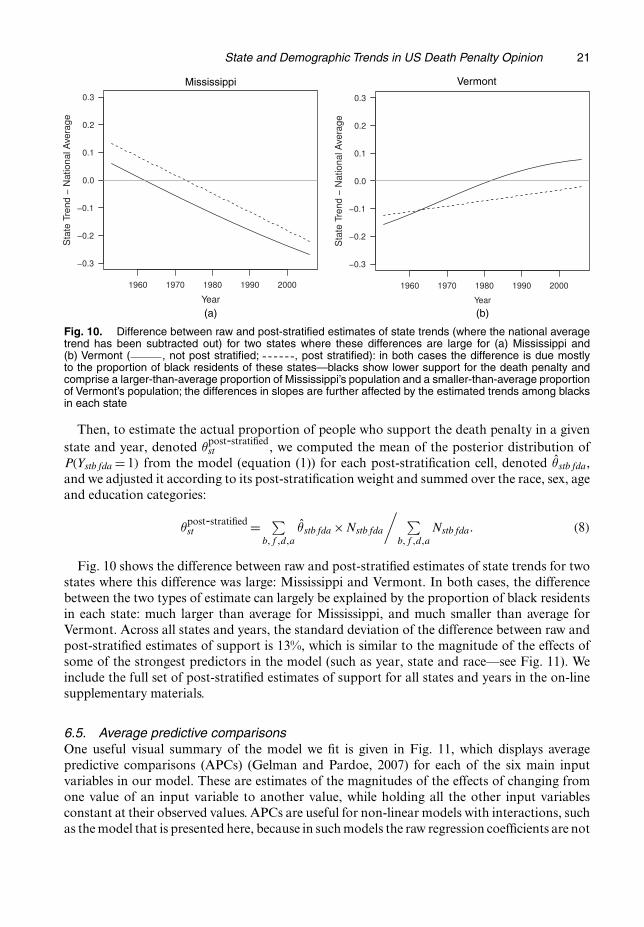
Fig. 10. Difference between raw and post-stratified estimates of state trends (where the national averagetrend has been subtracted out) for two states where these differences are large for (a) Mississippi and(b) Vermont ( , not post stratified; , post stratified): in both cases the difference is due mostlyto the proportion of black residents of these states—blacks show lower support for the death penalty andcomprise a larger-than-average proportion of Mississippi’s population and a smaller-than-average proportionof Vermont’s population; the differences in slopes are further affected by the estimated trends among blacksin each state

Then, to estimate the actual proportion of people who support the death penalty in a givenstate and year, denoted θ

post-stratifiedst , we computed the mean of the posterior distribution of

P.Ystbfda = 1/ from the model (equation (1)) for each post-stratification cell, denoted θ̂stbfda,and we adjusted it according to its post-stratification weight and summed over the race, sex, ageand education categories:

θpost-stratifiedst = ∑

b,f ,d,aθ̂stbfda ×Nstbfda

/ ∑b,f ,d,a

Nstbfda: .8/

Fig. 10 shows the difference between raw and post-stratified estimates of state trends for twostates where this difference was large: Mississippi and Vermont. In both cases, the differencebetween the two types of estimate can largely be explained by the proportion of black residentsin each state: much larger than average for Mississippi, and much smaller than average forVermont. Across all states and years, the standard deviation of the difference between raw andpost-stratified estimates of support is 13%, which is similar to the magnitude of the effects ofsome of the strongest predictors in the model (such as year, state and race—see Fig. 11). Weinclude the full set of post-stratified estimates of support for all states and years in the on-linesupplementary materials.

6.5. Average predictive comparisonsOne useful visual summary of the model we fit is given in Fig. 11, which displays averagepredictive comparisons (APCs) (Gelman and Pardoe, 2007) for each of the six main inputvariables in our model. These are estimates of the magnitudes of the effects of changing fromone value of an input variable to another value, while holding all the other input variablesconstant at their observed values. APCs are useful for non-linear models with interactions, suchas the model that is presented here, because in such models the raw regression coefficients are not


Fig. 11. Average predictive comparisons for the six input variables year, state, sex, race, age and education(these are estimates of the expected differences in death penalty support between the two respondents withdifferent values of one particular input variable, but similar values of all others): , point estimates; , 50%intervals for the differences; , 95% intervals

easily interpretable on the outcome scale (as opposed to linear regression without interactions,where the coefficients themselves act as APCs).

To compute the APC interval for the variable ‘year’, for example, we do as follows for eachposterior sample: for each respondent i = 1, : : : , n and for each year t = 1, : : : , T , compute thesquared difference in respondent i’s estimated death penalty support if he or she had respondedto the survey in year t, E.Yi|Xyear

i = t, Vi/, against the actual estimated support for respon-dent i, E.Yi|Xyear

i , Vi/, where Vi denotes the vector of values of the other five input variablesfor respondent i. Next, weight these T squared differences by a measure of how many of theother five input variables would probably be shared in common by a respondent in year t and arespondent in year X

yeari . This is done to downweight the squared differences between pairs

of years in which it would be unlikely to find two similar respondents in our data (see section4 of Gelman and Pardoe (2007) for more details). Last, take the square root of the mean ofthese weighted squared differences across all respondents. We did this for all 3000 posteriorsamples, for all six main variables, and plotted the resulting 50% and 95% APC intervals inFig. 11.

Our conclusion is that the survey year is associated with the most variation in death penaltysupport among all input variables, and that the estimated difference in probability of deathpenalty support between a randomly chosen respondent in our data and a similar respondentfrom a different year is about 18%. This estimate accounts for all the different ways in whichthe survey year affects death penalty support, from the national average time trend and yearlyeffects to the interactions between survey year and various demographic variables. The variablesthat account for the next two largest differences are state and race, and each accounts for abouta 14% difference in levels of support. Then, sex, education and age account for about 8%, 8%and 5% differences in death penalty support. In the case of all these variables, the 95% intervalshave a width of only about 1.5%.

7. Goodness-of-fit checks

We have already included plots of model estimates versus observed data in Figs 7 and 8, showingthe fit of the model with respect to trends among racial and gender-based groups. In this section,we display graphical checks of the fit of the model with respect to state trends, state–yearinteraction effects and trends among educational groups.


(a) (b)

Fig. 12. Differences between individual states and the national average over time on the probability scale,with estimates from the fitted model plotted with observed data (�, observed; �, fitted; - - - - -, state trend;

, regional trend; , national average) (the model-based estimates are of the estimated support foran individual of ‘average’ demographics; point sizes are proportional to the sample sizes for each state–year):(a) Massachusetts (northeast) (mean yearly sample size, 43; �, nD10;�, nD125); (b) Ohio (midwest) (meanyearly sample size, 85; �, nD12; �, nD180)

Fig. 12 illustrates the fit of the model with respect to the difference between the nationalaverage level of death penalty support and support in two specific states, Massachusetts andOhio, over time. For both states, the assumption of a linear trend explaining the differencesbetween state level opinion and national opinion seems reasonable. There may be some de-pendence from year to year for Ohio (especially in the late 1970s, when a group of about 4–5consecutive years were all above the estimated state trend line) but, on the whole, the inde-pendence assumption for the state–year interaction effects looks realistic. In years where moredata are observed (where the points are drawn in proportion to the sample size for that state–year), the estimated probabilities do not shrink as far towards the state trend line (1965, forexample). In years where there are few data, the estimated probabilities are pooled almost allthe way to the state trend line (Massachusetts in 2001, for example). Last, when there are nodata from a given year, the estimated percentages for a given state lie exactly on the state trendline.

We considered extending the model to allow for the effects of degree to vary across time.To investigate whether this would be likely to improve the fit of the model, we performed aposterior predictive check in which we simulated data for each respondent and compared thepredicted levels of support for each degree level over time, holding the other variables constantat their observed levels. The results are displayed in the five residuals plots in Fig. 2 of theon-line supplementary file ‘Supplementary-tables-and-figures.pdf’. There do not appear to beany patterns across time among the residuals in any of the degree level groups that would indicatethat our model is missing an important time trend. There appear to be influential points at theextremes of the x-axis for the high school degree category and the college degree category but,on the whole, the 95% intervals have approximately the correct level of coverage.

8. Out-of-sample predictions

To guide our model selection, we estimated the predictive accuracy of the five multilevel Bayesian


models that we fit in terms of the posterior mean of the deviance, where the deviance of modelm for posterior sample g, D

.g/m , is given by

D.g/m =−2

n∑i=1

[Yi log{P.Yi|θ.g/m /}+ .1−Yi/ log{1−P.Yi|θ.g/

m /}],

and θ.g/m is the vector of all model parameters for iteration g in model m. First, we randomly

divided our data set into a training set and a test set, containing 80% and 20% of the individualsurvey responses respectively. Since there is no widely agreed-on general rule for how to splitdata into training and test sets (Hastie et al., 2008), we choose a split (80:20) that lies within therange of previous analyses, e.g. Breiman (2001). We fitted each model to the training data andmade out-of-sample predictions on the test data.

Of the five multilevel Bayesian models that we fitted to the data, the fourth model, which wecall the main model, is that described in equation (1) and pictured by the directed acyclic graphin the on-line supplemental materials. The first, most basic model contained main effects for thefour demographic variables and state–year interaction terms, where the state–year interactionterms were centred at the sum of their respective year and state main effects, and each groupof main effect parameters had a prior mean of 0 and a half-t-prior distribution on its standarddeviation (the same as described in Section 4). The effective number of parameters, pD, forthis model, as estimated by the difference between the posterior mean of the log-likelihood andthe log-likelihood evaluated at the posterior mean of the parameters in the likelihood equation(Spiegelhalter et al., 2002), was about 500.

The second model contained state–year interaction terms, but this time with the exact sameprior structure as the main model—i.e. this model included state trends, state level variablesand an AR(1) prior distribution (with a linear component) for the yearly effects. The rest of thedemographic main effects were given the same structure and priors as in the first model—meansof 0, and half-t-prior distributions on their group level standard deviations. This model hadfewer effective parameters than the first model (about 434 compared with 500) because of thepartial pooling that is induced by the structured prior on the state–year interaction terms, andthe inclusion of state level variables (which help to induce even more pooling on the state-specificslopes and intercepts, decreasing the estimate of pD). This model fitted the training data worsethan the first model but made better predictions on the test set.

The third and fifth models were similar to the main model, with only minor modifications.The third model omitted the age–state slopes and was otherwise identical to the main model.This model performed slightly worse on the test set than the main model, and substantiallyworse on the training set. The fifth model included all the parameters in the main model andalso included four additional sets of two-way interactions: (sex, age), (sex, degree), (race, age)and (race, degree). The inclusion of each of these two-way interactions improved the predictiveperformance of the models fit during exploratory data analysis using ordinary least squaresregression, which is why we tried including them in a multilevel Bayesian model. The result oftheir addition to the main model, though, was a poorer fit than the main model on both thetraining and the test data sets.

It is possible that including only a subset of these additional interaction effects (or otherunexplored interactions that are not mentioned here) could have slightly improved the fit onthe test set, but our goal was not solely to make the best predictions, but rather to understandchanges in opinion over time (which is not a component of any of the additional interactioneffects in the fifth model), and to do so by emphasizing thorough graphical checks of thefit of the model. Thus, we proceeded with our analysis of the main model. Table 1 in the


Table 1. Post-stratified estimates of levels of support among thefour race–sex subgroups over time

Race–sex subgroup Estimates for the following years:

1955 1965 1975 1985 1995 2005

Non-black men 0.70 0.58 0.74 0.85 0.85 0.79Non-black women 0.61 0.47 0.63 0.77 0.78 0.69Black men 0.50 0.33 0.46 0.59 0.56 0.42Black women 0.42 0.27 0.39 0.54 0.52 0.40

on-line supplementary file ‘Supplementary-tables-and-figures.pdf’ contains details of thedeviance, effective number of parameters and deviance information criterion of the multilevelBayesian models that we fitted.

9. Discussion

We fitted a multilevel Bayesian model to 58253 individual responses to the question ‘Are youin favor of the death penalty for persons convicted of murder?’ by using data from a 54-yeartime span and including demographic and state level variables. The use of a structured priordistribution on the yearly effects allowed us to estimate simultaneously their variation, whilealso estimating various main effects, trends and interaction effects that shed new light on certainrelationships between demographic variables and death penalty support, and on trends in deathpenalty support among states.

We found that blacks have decreased their support over time dramatically compared withnon-blacks, with the support among black men showing a faster relative decrease, on average,than among black women. This pattern was previously difficult to identify because of nationwidefluctuations in death penalty support over time (see Fig. 3) and sampling variation. Hanley (2008)pointed out that support was higher in the 1990s than in the 1970s among many subgroups ofthe population, including blacks, despite high profile court cases in the late 1980s that foundevidence for bias against blacks in death sentencing (which presumably would result in lowersupport among blacks). Although support among blacks was higher in the 1990s than in the1970s in absolute terms, this increase in support was observed for both blacks and non-blacks(i.e. it can be explained by the increased national support for the death penalty in the 1990s).According to our model, the relative support among blacks compared with non-blacks was inthe middle of a steady decline—one that was steeper, on average, for black males than blackfemales (see Fig. 7). Further, Hanley (2008) claim that

‘since 1990 black men have been more supportive of the death penalty than black women, after a periodof fluctuation in the late 1970s and 1980s’.

Whether or not this fluctuation was real (or just the result of sampling variability), our analysisshows that the gap in support among black men compared with black women is shrinking,on average, from a difference of about 10% in the 1950s to a difference of just 1% in the mid-2000s. For a summary of levels of support among race–sex subgroups over time, in additionto Fig. 7, which plots estimated relative trends in support among subgroups, Table 1 containspost-stratified estimates of absolute levels of support among race–sex subgroups.


We also found that death penalty support has grown faster in states where support forRepublican presidential candidates has grown during the past 50 years, and average support overtime has been higher in states where the death penalty has been legal for a larger proportion ofthe past 50 years. In future work, each of these state level variables could be refined or modifiedto discover additional, potentially stronger associations between state level partisan support,state level policy and individual death penalty support. For example, partisan support at thestate level for governors or state legislatures may be more strongly associated with death penaltysupport than partisan presidential support. Since partisan support is also a dynamic process,a joint model for partisan support and death penalty support could reveal new associationsbetween these two phenomena over time. Also, rather than looking only at whether the deathpenalty is legal in a given state, it is possible that other state level variables such as the crimerate, the number of death sentences or the number of executions carried out in a given state andyear could be associated with individual level support for the death penalty in that state.

We chose to model state-specific slopes and intercepts as being centred near their regionalmeans, according to a US-census-based four-region breakdown of the 51 states. We chose to usethis four-region breakdown of the states because it is relatively simple, well known and oftencited in studies of public opinion by region in the USA (Gelman, 2008; Lax and Phillips, 2009b).Alternative groupings of states into regions, or alternative models to allow for correlationsbetween states, however, could be of interest for future work. The US census contains alternativeregional groupings of the states into nine groups of states, which might allow for more variationbetween regions than what we observed with our model. One could also fit a model in whichstate effects are correlated with the effects of neighbouring states, or one could fit a latent classmodel, to infer groups of similarly opinionated states from the data, rather than using predefinedregions. Such an investigation into correlations between groups of states would be interestingbut was beyond the scope of this paper.

Another modification to the model that might be useful in future investigations would beto allow for dependence of the state–year effects across time within states. If each state’s state–year effects followed an AR(1) model, for example, then perhaps the varying level of dependencefrom year to year for each state would provide new information about how public opinion variesacross time within states. For example, the opinions of respondents in some states might be verystable, if that state had highly auto-correlated state–year effects. In contrast, their opinionsmight be very prone to yearly swings, if that state had low or negative auto-correlation betweenstate–year effects, perhaps in reaction to local events or changes in policy that were related tothe death penalty.

Future models could also include additional survey data and, if necessary, model differencesin data collected by different organizations. One could also attempt to gather more demographicvariables for each respondent, such as political party affiliation, income or religion, to under-stand better the factors that predict attitudes on this issue.

Last, regarding the type of model that we fitted, it could also make sense to consider non-parametric regression methods such as Bayesian additive regression trees (Chipman et al., 2010),perhaps in combination with existing regression models to pull out any structure in the databeyond what is captured by our logistic regression.

To return to the political questions that motivated this work: public opinion is, presumably,both a cause and a consequence of policies on capital punishment. To study these connections,researchers need measures of state level opinion. In a study of state level attitudes on gay rights,Lax and Phillips (2009b) showed a level of responsiveness of legislators’ policy to opinion thatwas surprising given some of the earlier literature on state politics. The present research goesfurther by modelling trends at the state level by using sparse data.


10. Supplementary materials

The on-line supplementary materials comprise the following files:

(a) DAG.pdf, a directed acyclic graph of the full model;(b) Adjusted-parameters.pdf, a description of the calculations to derive the adjusted param-

eters;(c) Supplementary-figures-and-tables.pdf, a plot of the state-specific slops and intercepts by

region, residuals of support by degree and tables containing model comparison statisticsand state effects;

(d) estimates.RData, interval estimates of the level of support for the death penalty for eachpossible combination of (state, year, race, sex, degree, age);

(e) varnames.RData, names of variables that correspond to the dimensions of the array inthe file estimates.RData;

(f) poststrat.RData, post-stratified estimates of the level of support for the death penalty bystate and year.

Acknowledgements

Most of this work was completed while the first author was a postdoctoral student at ColumbiaUniversity.

This research was supported in part by National Science Foundation grant 1023189. Theauthors also thank the Roper Center for Public Opinion Research for use of the iPoll archive.

References

Baumgartner, F. R., De Boef, S. L. and Boydstun, A. E. (2008) The Decline of the Death Penalty and the Discoveryof Innocence. Cambridge: Cambridge University Press.

Breiman, L. (2001) Statistical modeling: the two cultures. Statist. Sci., 16, 199–231.Chipman, H. A., George, E. I. and McCulloch, R. E. (2010) Bart: Bayesian additive regression trees. Ann. Appl.

Statist., 4, 266–298.Datta, G. S., Lahiri, P., Maiti, R. and Lu, K. L. (1999) Hierarchical bayes estimation of unemployment rates for

the states of the U.S. J. Am. Statist. Ass., 94, 1074–1082.Ellsworth, P. C. and Gross, S. R. (1994) Hardening of the attitudes: Americans’ views on the death penalty. J. Socl

Iss., 50, no. 2, 19–52.Erikson, R. (1976) The relationship between public opinion and state policy: a new look based on some forgotten

data. Am. J. Polit. Sci., 20, 25–36.Erskine, H. (1970) The polls: capital punishment. Publ. Opin. Q., 34, 290–307.Fox, J. A., Radelet, M. L. and Bonsteel, J. L. (1991) Death penalty opinion in the post-Furman years. New Yrk

Univ. Rev. Law Socl Change, 28, 499–528.Franklin, C. (2001) Pre-election polls in nation and state: a dynamic bayesian hierarchical model. Technical Report.

University of Wisconsin, Madison.Gelfand, A. E. and Sahu, S. K. (1999) Identifiability, improper priors, and Gibbs sampling for generalized linear

models. J. Am. Statist. Ass., 94, 247–253.Gelman, A. (2008) Red State, Blue State, Rich State, Poor State: Why Americans Vote the Way They Do. Princeton:

Princeton University Press.Gelman, A. and Hill, J. (2007) Data Analysis using Regression and Multilevel/Hierarchical Models. Cambridge:

Cambridge University Press.Gelman, A. and Pardoe, I. (2007) Average predictive comparisons for models with nonlinearity, interactions, and

variance components. Sociol. Methodol., 37, 23–51.Gelman, A. and Rubin, D. (1992) Inference from iterative simulation using multiple sequences. Statist. Sci., 7,

457–472.Hanley, J. (2008) The death penalty. In Public Opinion and Constitutional Controversy, ch. 5, pp. 108–138. Oxford:

Oxford University Press.Hastie, T., Tibshirani, R. and Friedman, J. (2008) The Elements of Statistical Learning: Data Mining, Inference,

and Prediction, vol. 2. New York: Springer.


Lax, J. R. and Phillips, J. H. (2009a). How should we estimate public opinion in the states? Am. J. Polit. Sci., 53,107–121.

Lax, J. R. and Phillips, J. H. (2009b). Gay rights in the states: public opinion and policy responsiveness. Am. Polit.Sci. Rev., 103, 367–386.

Norrander, B. (2000) The multi-layered impact of public opinion on capital punishment implementation in theamerican states. Polit. Res. Q., 53, 771–793.

Plummer, M. (2003) Jags: a program for analysis of bayesian graphical models using gibbs sampling.3rd Int. Wrkshp Distributed Statistical Computing, Vienna, Mar. 20th–22nd. (Available from http://mcmc-jags.sourceforge.net.)

Rao, J. N. K. (2003) Small Area Estimation. New York: Wiley.Ruggles, S., Alexander, J. T., Genadek, K., Goeken, R., Schroeder, M. B. and Sobek, M. (2010) Integrated public

use microdata series: Version 5.0. Database. University of Minnesota, Minneapolis.Schuman, H. and Presser, S. (1981) Questions and Answers in Attitude Surveys: Experiments on Question Form,

Wording, and Context. New York: Sage.Spiegelhalter, D. J., Best, N. G., Carlin, B. P. and van der Linde, A. (2002) Bayesian measures of model complexity

and fit (with discussion). J. R. Statist. Soc. B, 64, 583–639.Vidmar, N. and Ellsworth, P. (1974) Public opinion and the death penalty. Stanfrd Law Rev., 26, 1245–1270.

Supporting informationAdditional ‘supporting information’ may be found in the on-line version of this article.

hierarchical models for estimating state and …gelman/research/published/a12052_shirley.pdf ·...

Documents