hierarchical algorithms for causality retrieval in atrial...

IEEE JOURNAL OF BIOMEDICAL AND HEALTH INFORMATICS, VOL. 23, NO. 1, JANUARY 2019 143

Hierarchical Algorithms for Causality Retrieval inAtrial Fibrillation Intracavitary Electrograms

David Luengo , Member, IEEE, Gonzalo Rıos-Munoz , Vıctor Elvira, Member, IEEE, Carlos Sanchez,and Antonio Artes-Rodrıguez , Senior Member, IEEE

Abstract—Multichannel intracavitary electrograms(EGMs) are acquired at the electrophysiology laboratoryto guide radio frequency catheter ablation of patientssuffering from atrial fibrillation. These EGMs are used bycardiologists to determine candidate areas for ablation(e.g., areas corresponding to high dominant frequenciesor complex fractionated electrograms). In this paper,we introduce two hierarchical algorithms to retrieve thecausal interactions among these multiple EGMs. Bothalgorithms are based on Granger causality, but othercausality measures can be easily incorporated. In bothcases, they start by selecting a root node, but they differon the way in which they explore the set of signals todetermine their cause-effect relationships: either testingthe full set of unexplored signals (GS-CaRe) or performinga local search only among the set of neighbor EGMs(LS-CaRe). The ensuing causal model provides importantinformation about the propagation of the electrical signalsinside the atria, uncovering wavefronts and activationpatterns that can guide cardiologists towards candidateareas for catheter ablation. Numerical experiments, on bothsynthetic signals and annotated real-world signals, showthe good performance of the two proposed approaches.

Index Terms—Electrocardiography, intracavitary electro-grams, atrial fibrillation, radio frequency ablation, Grangercausality.

Manuscript received June 15, 2017; revised November 8, 2017 andJanuary 10, 2018; accepted February 3, 2018. Date of publication Febru-ary 12, 2018; date of current version January 2, 2019. This work wassupported in part by the BBVA Foundation through “I Convocatoria deAyudas a Investigadores, Innovadores y Creadores Culturales” (MG-FIAR project), in part by the Spanish “Ministerio de Industria, Economıay Competitividad” through the MIMOD-PLC (TEC2015-64835-C3-3-R)and ADVENTURE (TEC2015-69868-C2-1-R) projects, and in part bythe Comunidad de Madrid through project CASI-CAM-CM (S2013/ICE-2845). (David Luengo and Gonzalo Rıos-Munoz contributed equally tothis work.) (Corresponding author: David Luengo.)

D. Luengo is with the Department of Signal Theory and Communica-tions, Universidad Politecnica de Madrid, Madrid 28031, Spain (e-mail:[email protected]).

G. Rıos-Munoz and A. Artes-Rodrıguez are with the Department ofSignal Theory and Communications, Universidad Carlos III de Madrid,Madrid 28903, Spain, and also with Gregorio Maranon Health ResearchInstitute, Madrid 28009, Spain (e-mail: [email protected]; [email protected]).

V. Elvira is with the IMT Lille Douai, Universite de Lille, Lille 59000,France, and also with CRIStAL Laboratory (UMR 9189), Villeneuve-d’Ascq 59655, France (e-mail: [email protected]).

C. Sanchez is with the Defense University Centre (CUD) of the Gen-eral Military Academy of Zaragoza (AGM), the Biosignal Interpretationand Computational Simulation (BSICoS) Group, Aragon Institute of En-gineering Research (I3A), Universidad de Zaragoza, Zaragoza 50009,Spain, and also with Centro de Investigacin Biomedica en Red (CIBER-BBN), Madrid 28029, Spain (e-mail: [email protected]).

Digital Object Identifier 10.1109/JBHI.2018.2805773

I. INTRODUCTION

A TRIAL fibrillation (AF) is a cardiac pathology charac-terized by a rapid and unsynchronized contraction of the

atria. AF is the most common cardiac arrhythmia in clinicalpractice [1], having reached epidemic proportions: one out offour people over 40 years old are predicted to suffer from AFthroughout their lifetime [2]. Although AF is not deadly per se,it causes a substantial discomfort on patients, results in a largenumber of hospitalizations and is an important risk factor forother pathologies like sudden death [3] or stroke [4]. However,the underlying causes for the initiation and maintenance of AFare still not fully understood, and several hypotheses have beenproposed [5], [6]. The prevailing hypothesis for AF mainte-nance still relies on the existence of multiple wavelets randomlypropagating through the atria [7], [8]. More recently it has beenhypothesized that stable spatio-temporal re-entrant waves (ro-tors) may be responsible for AF initiation and maintenance [9].According to this theory, ablating those specific areas of themyocardium should lead to AF termination. Consequently, ra-dio frequency (RF) ablation, where an RF catheter is introducedinside the heart and used to ablate potentially arrhythmogeneticareas, is increasingly used. This approach has shown promisingresults for paroxysmal AF patients, with success rates around70–80% by performing pulmonary vein isolation (PVI), but hasnot been so effective for persistent AF [10]. In this case, otherablation strategies (e.g., ablating areas with complex fraction-ated EGMs [11] or high dominant frequencies [12]) have beentested, but their results are still unsatisfactory in many cases.1

The lack of satisfactory performance of RF ablation strategiesfor some patients is our main motivation. We believe that thereis an urgent need of more advanced signal processing and ma-chine learning methods that can assist cardiologists during RFablation therapies. These techniques should focus on determin-ing the direction of information transfer in the multiple EGMsrecorded in the electrophysiology laboratory. This informationwill help both to better understand the propagation of the actionpotential (AP) inside the atria of AF patients and to identify can-didate sites for RF ablation. With these goals in mind, Grangercausality (G-causality or GC) is a well established methodol-ogy to infer causal relations among multiple time series [15].

1Complex fractionated EGMs are electrograms that do not exhibit the quasi-periodic shape of regular electrograms, but a much more complex and irregularshape [13]. The dominant frequency (DF) corresponds to the highest peak ofthe frequency spectrum measured in a certain area inside the atria [14].

2168-2194 © 2018 IEEE. Personal use is permitted, but republication/redistribution requires IEEE permission.See http://www.ieee.org/publications standards/publications/rights/index.html for more information.

https://orcid.org/0000-0001-7407-3630

https://orcid.org/0000-0003-2446-3045

https://orcid.org/0000-0001-6540-7109

144 IEEE JOURNAL OF BIOMEDICAL AND HEALTH INFORMATICS, VOL. 23, NO. 1, JANUARY 2019

TABLE ISUMMARY OF THE MAIN NOTATION USED IN THE DEFINITION OF THE HIERARCHICAL GRANGER CAUSALITY ALGORITHM

Variable Description

xq [n] Observed signals (1 ≤ q ≤ Q, 0 ≤ n ≤ N − 1).M�q Maximum delay in the prediction from the �-th to the q-th signal. Can be user-defined or determined automatically.x� [n] Vector containing all the previous M�q samples of x� [n]: x� [n] = [x� [n − 1], . . . , x� [n − M�q ]]�.α�q [n] Coefficients of the linear predictor from the �-th to the q-th signal.α�q Vector containing all the coefficients of the linear predictor from the �-th to the q-th signal: α�q = [α�q [1], . . . , α�q [M�q ]]�.G�→q Pairwise G-causality strength from the �-th signal to the q-th signal.G Pairwise G-causality strength matrix s.t. G�,q = G�→q for 1 ≤ �, q ≤ Q.C�q Pairwise G-causality connectivity from the �-th signal to the q-th signal, C�q = χp (G�→q ).C Pairwise G-causality connection matrix s.t. C�,q = [[χ(G�→q ) ≥ γp ]], i.e., C�,q = 1 if χ(G�→q ) ≥ γp and C�,q = 0 otherwise.γp Threshold used to determine whether a causal link exists or not. It is a function of the user-defined p-value.G�→q |I Conditional G-causality strength from the �-th signal to the q-th signal given the set of nodes in I.GI Conditional G-causality strength matrix s.t. GI (�, q) = G�→q |I .C�→q |I Conditional G-causality connectivity from the �-th signal to the q-th signal given the set of nodes in I.

CI Conditional G-causality connection matrix s.t. CI (�, q) = [[χ(G�→q |I

)≥ γp ]].

Cq = cand{iq } Set of candidate sons of the q-th node (1 ≤ q ≤ Q).Sq = son{iq } Set of sons of the q-th node (1 ≤ q ≤ Q).Pq = pa{iq } Set of parents of the q-th node (1 ≤ q ≤ Q).

Several authors have investigated the inference of causality re-lationships among different biomedical signals [16], [17]. Inparticular, causality discovery tools have been extensively usedin neurology [15], and GC has been used to investigate therelationship between several physiological time series (heartperiod, arterial pressure and respiration variability) [18], [19].The use of partial directed coherence to investigate propagationpatterns in intra-cardiac signals was considered in [20], [21],whereas GC maps have been built in [22]–[24]. However, all ofthese approaches are based on the standard approach to causal-ity discovery, i.e., computing the pairwise or full-conditionalG-causality as described in Section II. More recently, [25] pro-posed alternative multi-variate causality measures that involvethe computation of GC conditioned only on neighbor nodes.

In this paper, a hierarchical framework for causality retrievalin EGMs is described. The first stage of the proposed method-ology consists of finding the EGM having the “strongest” GClinks with other EGMs and selecting it as the root node. Theremaining nodes are then processed sequentially, starting fromthe set of candidate children of the root node. Two alterna-tive algorithms are proposed for this purpose: global searchcausal retrieval (GS-CaRe) and local search causal retrieval(LS-CaRe). GS-CaRe processes the candidate children of thecurrent node sequentially according to their causal strength,accepting them as true children if their GC is statisticallysignificant conditioned on all the previously accepted children.LS-CaRe also processes the candidate children sequentially, butonly takes into account the neighbor nodes, thus avoiding manyfalse alarms. An exhaustive evaluation of the proposed algo-rithms has been performed, using both synthetic signals andannotated real-world signals from AF patients acquired at theelectrophysiology laboratory of Hospital General UniversitarioGregorio Maranon (HGUGM). Note that the GS-CaRe algo-rithm was already described in [26], [27]. With respect to [26],[27], a completely novel algorithm (LS-CaRe) is proposed, andan exhaustive set of simulations (using synthetic and real data)are performed to validate both algorithms.

The rest of the paper is organized as follows. Firstly,Section II provides an introduction to Granger causality, de-scribing both pairwise and conditional causality. The notationused throughout the text is also summarized here in Table I.Then, Section III describes the two hierarchical causality dis-covery algorithms proposed: GS-CaRe and LS-CaRe. This isfollowed by Section IV, where numerical experiments (usingboth synthetic and real data) are used to validate the developedalgorithms. Finally, the paper is closed in Section V with adiscussion that includes potential future lines.

II. GRANGER CAUSALITY

A. Pairwise Causality

Let us assume that we have N samples of a multi-variatetime series composed of Q interrelated signals, xq [n] for q =1, . . . , Q and n = 0, 1, . . . , N − 1. Granger causality measuresthe increase in predictability on the future outcome of a signal,xq [n], given the past values of another signal, x� [n] with � �= q,with respect to (w.r.t.) the predictability achieved by taking intoaccount only past values of xq [n] [15], [28]. In short, G-causalitydetermines whether past values of x� [n] can be useful to forecastfuture values of xq [n] or not.

In order to provide a rigorous formulation of GC, let us definethe linear autoregressive (AR) predictor for xq [n] given its pastsamples (i.e., the q-th self-predictor) as

xq [n] = xq→q [n] =M∑

m=1

αqq [m]xq [n − m] = α�qqxq [n], (1)

where M is the order of the predictor, obtained typically us-ing some penalization for model complexity to avoid over-fitting [29]; αqq [m] are the coefficients of the model; αqq =[αqq [1], . . . , αqq [M ]]� and α�

qq denotes the transpose of αqq ;and xq [n] = [xq [n − 1], . . . , xq [n − M ]]�. Similarly, let us de-fine the linear AR predictor for xq [n] given the past samplesof both xq [n] and x� [n] (i.e., the cross-predictor from the �-th

LUENGO et al.: HIERARCHICAL ALGORITHMS FOR CAUSALITY RETRIEVAL IN ATRIAL FIBRILLATION INTRACAVITARY ELECTROGRAMS 145

signal to the q-th signal) as

x�→q [n] = α�qqxq [n] + α�

�qx� [n] = xq [n] + α��qx� [n], (2)

where α�q = [α�q [1], . . . , α�q [M ]]�; x� [n] = [x� [n − 1], . . . ,x� [n − M ]]�; and xq [n] is given by (1).

The residual errors of these two predictors in (1) and (2)can now be defined as εq [n] = xq [n] − xq [n] and ε�→q [n]= xq [n] − x�→q [n], respectively. The pairwise G-causalitystrength is then measured by the logarithm of the ratio of thetwo variances of the residuals [30]:

G�→q = lnVar(εq [n])

Var(ε�→q [n]). (3)

Note that Var(ε�→q [n]) ≈ Var(εq [n]) when x� [n] doesnot provide any useful information w.r.t. xq [n], whereasVar(ε�→q [n]) < Var(εq [n]) if x� [n] allows us to improve theprediction of xq [n]. Hence, 0 ≤ G�→q < ∞, with larger valuesof G�→q indicating a stronger evidence of causality from � to q.Using these pairwise values, we can build a pairwise G-causalitystrength matrix, G, such that its (�, q)-th entry is given by2

G�,q =

{G�→q , � �= q;

0, � = q.(4)

Finally, it is important to remark that we should add a causal-ity link from � to q only when the decrease in the residual’snoise variance from (1) to (2) is statistically significant. In or-der to construct this causality graph, we define the pairwiseG-causality connection matrix, C, whose (�, q)-th element is

C�,q =

{1, χ(G�→q ) ≤ γ;

0, χ(G�→q ) > γ,(5)

where χ(G�→q ) denotes some appropriate statistic and γ isthe threshold value (i.e., significance level) used to determinewhether the value of G�→q is statistically significant. In orderto retrieve the potential causality link between two nodes, weresort to p-values, and thus we denote γ = γp [31].3 The typ-ical values of p in biomedical engineering which will be usedhere are p = 0.05, p = 0.01 or p = 0.001. Finally, for the sakeof simplicity we will use the following short-hand notation forC�,q in (5):

C�,q = [[χ(G�→q ) ≤ γp ]], (6)

where [[LC]] = 1 if the logical conditionLC is true and [[LC]] = 0otherwise (i.e., if LC is false), whereas γp is the threshold valueobtained from the corresponding user-defined p-value.

2Note that Var(εq→q [n]) = Var(εq [n]), since xq [n] = xq→q [n], and thusthe definition in (4) is consistent with (3), since Gq→q [n] = ln 1 = 0.

3Let us note that some alternative and more complicated approaches thanp-values have been proposed in the literature [32]. However, p-values are sim-ple to understand and set by the users, their use is widespread in biomedicalapplications (as well as in other scientific areas), and they are enough for ourpurposes. Indeed, we have tested several values of p in the simulations (seeSection IV), noticing that the value of p has little influence on the results, aslong as it is small enough (i.e., p ≤ 0.05).

B. Conditional Causality

Unfortunately, pairwise GC is unable to discriminate betweendirect causation (e.g., x1 [n] → x3 [n]) and indirect causation(e.g., x1 [n] → x2 [n] → x3 [n]). In both cases, the pairwise G-causality approach would lead to C1,3 = 1, implying that x1 [n]has caused x3 [n]. However, when building the causality networkwe are only interested in direct causes, since all the spuriouslinks created by indirect causes may obscure the flow of infor-mation among signals. In order to avoid these undesired linksreturned by pairwise causality, conditional G-causality was in-troduced in [30]. In short, conditional GC attempts to determinewhether x� [n] has caused xq [n] given another set of intermediatesignals.

In order to provide a precise mathematical definition of con-ditional GC, let us define the set containing the indexes of theconditioning variables as I. Following a similar procedure asbefore, we define the conditional self-predictor

xq |I [n] = α�qqxq [n] +

∑

r∈Iα�

rqxr [n], (7)

where αrq = [αrq [1], . . . , αrq [M ]]� and xr [n] = [xr [n − 1],. . . , xr [n − M ]]� for all r ∈ I, and the conditional cross-predictor from the �-th signal (with � /∈ I) to the q-th output

x�→q |I [n] = α�qqxq [n] +

∑

r∈Iα�

rqxr [n] + α��qx� [n]

= xq |I [n] + α��qx� [n]. (8)

Now, by defining the residual errors from the conditional pre-dictors as εq |I [n] = xq [n] − xq |I [n] and ε�→q |I [n] = xq [n] −x�→q |I [n], the conditional G-causality strength can be defined,in a similar way to (3), as

G�→q |I = lnVar(εq |I [n])

Var(ε�→q |I [n]). (9)

Again, 0 ≤ G�→q |I < ∞, with larger values of G�→q |I indicat-ing a stronger evidence of causality from � to q given the set ofsignals in I; and we define two conditional connection/strengthGC matrices, GI and CI , whose (�, q)-th elements are, respec-tively, G�,q |I = G�→q |I and C�,q |I = [[χ(G�→q |I) ≤ γp ]].

Note that the pairwise GC connection/strength matri-ces are unique, whereas many conditional GC connec-tion/strength matrices can be constructed. The most usualsituation is setting I = S¬� = {1, . . . , � − 1, � + 1, . . . , Q} ={1, . . . , Q} \ {�} and constructing the full conditional GC con-nection/strength matrices asG�,q |S¬�

= G�→q |S¬�andC�,q |S¬�

=[[χ(G�→q |S¬�

) ≤ γp ]], respectively. However, conditional causal-ity can also be used to build hierarchical models by condition-ing on specific sets of nodes in a structured way, as describedin Section III.

III. HIERARCHICAL GRANGER CAUSALITY FOR

INTRACAVITARY ELECTROGRAMS

On the one hand, pairwise GC may provide misleading re-sults, as discussed in Section II-A. On the other hand, the“brute-force approach” to conditional causality (i.e., applying


conditional causality on the whole data set all at once) may ob-scure some of the existing relationships. Let us consider againthe three-node causal network x1 [n] → x2 [n] → x3 [n]. Now,by applying the full-conditional GC approach we would typ-ically obtain a single dependence relation: G1→2|3 = 1. Theother desired link, x2 → x3 , would typically not be included,since G2→3|1 = 0 unless a very short lag (M ) is used to ensurethat only signals from neighbor nodes are taken into account(i.e., that the contribution of x1 [n − 1], . . . , x1 [n − M ] to theprediction of x3 [n] is negligible).

In this paper we propose two hierarchical methods that areable to exploit the advantages of both approaches while mini-mizing their drawbacks. Both algorithms start by searching forthe node with the “strongest” G-causality links with the remain-ing nodes and selecting it as the root node.4 Then, the childrenof the root node are processed, adding new causality links ifthe corresponding causality test is passed. This process is re-peated iteratively until there are no more nodes to process anda poly-tree has been constructed. The assumed premises are thefollowing:

1) No feedback links can exist from lower nodes to highernodes in the hierarchy. This restriction is a consequenceof the refractory period of the AP: a period of time fol-lowing the excited phase when additional stimuli evokeno substantial response [33].5

2) Causal interactions typically occur between neighbornodes. This behavior is due to the continuous propagationof the waveform through the cardiac tissue.

In the sequel, we first describe the common initial step (i.e.,the selection of the root node) and then we detail the two hierar-chical causality algorithms proposed: GS-CaRe and LS-CaRe.

A. Initialization: Selecting the Root Node

The initialization stage, which is common for both the GS-CaRe and the LS-CaRe algorithms, seeks to find the optimalroot node for the causal graph. This is done by computing thepairwise GC among all nodes and selecting the one with the“strongest” causal connections to other nodes. More precisely,the steps performed to select the root node are the following:

1) Compute Gq→� and G�→q (for �, q = 1, . . . , Q − 1), andset the corresponding entries in G and C.

2) Calculate the GC strength of the q-th node (q =1, . . . , Q − 1) as the sum of the strength of its causal

4Note that the proposed framework essentially tries to identify the propagationdirection of the AP. In order to do so, we propose a hierarchical approachbased on Granger causality (although other causality measures could also beused) to measure the direction of the transfer of information throughout theavailable electrodes. In this setting, the root node becomes the entry point ofthe waveform to the set of electrodes, and thus it is essential to determine thedesired propagation direction.

5Note that this assumption holds regardless of the type of catheter used, aslong as the measurements taken by this catheter are all concentrated in a certainarea of the atria (i.e., it may not hold for basket catheters that try to cover all ofthe atria). The only exception for the circular catheter used in the experiments(see Section IV) concerns the initial and final points in the hierarchy when wehave circular dependencies like the ones shown in Fig. 3(p), (n), and (o). In thiscase our algorithm is unable to discover this last connection, and thus wouldalways have at least one missing link.

Fig. 1. Flow diagram of the GS-CaRe algorithm.

links to the remaining nodes:

gq =Q∑

�=1

Gq ,� =Q∑

�=1

Gq→� . (10)

Calculate also the number of links for each node as

Kq =Q∑

�=1

Cq ,� =Q∑

�=1

[[χ(Gq→�) ≤ γp ]]. (11)

3) Determine the node with the largest number of outgoingcausal links (i.e., links from that source node to someother sink node), selecting it as the root node:6

i1 = arg max1≤q≤Q

Kq , (12)

with gq being used only to discriminate among nodeswith identical values of Kq .

B. Global Search Hierarchical Algorithm (GS-CaRe)

The GS-CaRe algorithm was initially proposed in [26] andlater on refined in [27]. Fig. 1 shows the flow diagram of theGS-CaRe algorithm. After the selection of the root node, asdescribed in Section III-A, GS-CaRe sets the root node as thecurrent node and processes this current node (e.g., node i) re-cursively as shown in Fig. 1:

6In [26], the root node was obtained by maximizing gq instead of Kq , butwe have observed that this can lead to an erroneous selection of the root nodewhen a single very strong causal connection (i.e., a single very large value ofG) dominates over the rest.


Fig. 2. Flow diagram of the LS-CaRe algorithm.

� Finds the candidate children of the current node, Ci =cand{i} = {� : Ci,� = 1}, using pairwise GC.7

� Sorts the candidate children according to their pairwiseGC strength, in such a way that Gi→Ci (1) ≥ Gi→Ci (2) ≥Gi→Ci (3) ≥ . . .

� Finds the true children sequentially using conditional GC,starting with the “strongest” candidate and conditioningon all the previously accepted true children.

If the current node has some true children, the strongest one isselected as the current node, removed from the true children listand the aforementioned process is repeated again. It the currentnode does not have any true children (either because they havealready been processed or because the end of the causality chainhas been reached), then the parent of the current node is set as thecurrent node and the process is repeated again. The algorithmends when the current node is again the root node and doesnot have true children to process anymore. At the end of thisprocess, GS-CaRe returns the strength/connection GC matrices,G and C, which define a poly-tree with its children and parents.

C. Local Search Hierarchical Algorithm (LS-CaRe)

Fig. 2 shows the flow diagram of the LS-CaRe algorithm.LS-CaRe processes the nodes directly according to their causalstrength (starting from the root node, which is the “strongest”one), considering only causal links among neighbors up to amaximum user-defined distance, dmax . First of all, let us define

7Note that the search for candidate children is only performed on the currentlyunprocessed nodes. See [26] or [27] for further details.

the distance among nodes as

d(�, q) = min{((� − q))Q , ((q − �))Q}, (13)

for any �, q ∈ {1, 2, . . . , Q} and with ((·))Q denoting the mod-ulo operation, i.e., for any three integer numbers m, k and Q,m = ((k))Q ⇔ k = rQ + m, where r and m are the only inte-gers such that −∞ < r < ∞ and 0 ≤ m ≤ Q − 1. Then, usingthe Kq computed in Section III-A, construct an ordered set ofnodes, I = {i1 , i2 , . . . , iQ} with i1 being the root node, suchthat K� ≥ Kq for all � < q.8 Initialize the set of neighbors of

each node by including only the own nodes (i.e., N (0)q = {q}

for q = 1, . . . , Q). Set q = 1 and d = 1. Now, the LS-CaRealgorithm proceeds in the following way:

1) Update the set of neighbors by including those neighborsat distance d from iq , i.e., set N (d)

q = N (d)q ∪ L(d)

q with

L(d)q = {� : d(iq , �) = d, � = 1, . . . , Q}. (14)

Hence,N (d)q includes now all those nodes whose distance

to node iq is lower or equal than d.

2) For any node � ∈ L(d)q , add an edge from iq to � if Ciq →� =

1 and the following two conditions are fulfilled:a) There is no connection from any of the neigh-

bors in N (d−1)q to/from iq . Mathematically,

defining

E (d)q =

∑

�∈N (d −1 )q

(C�→iq

+ Ciq →�

), (15)

an edge can only be added if E (d)q = 0. This con-

dition implies that edges should not be added tonodes far away if connections to closer nodes al-ready exist.

b) The �-th node is not already connected, i.e.,∑Qj=1 Cj→� = 0 or

∑Qj=1 C�→j = 0.

3) If q < Q, then set q = q + 1 and return to step 1.Otherwise, set q = 1 and check d. If d < dmax , setd = d + 1 and return to step 1.

At the end of this process, GS-CaRe returns again thestrength/connection GC matrices, G and C, for the whole setof nodes.

IV. NUMERICAL EXPERIMENTS

In this section, we first define the performance measures thatwill be used in Section IV-A. Then, we describe the numericalexperiments performed using synthetic data in Sections IV-Band IV-C. Finally, the validation using annotated real data isprovided in Section IV-D. In order to implement the four algo-rithms tested in this section (GS-CaRe, LS-CaRe, the pairwiseapproach and the full-conditional method), we have used theGranger causal connectivity (GCCA) toolbox [34].

8As indicated in Section III-A, when K� = Kq for two nodes � and q, weuse g� and gq to break the tie.


A. Methods and Performance Measures

In order to gauge the performance of the two novel hierar-chical algorithms (LS-CaRe and GS-CaRe), we compare themagainst the following methods:

� Pair: pairwise causality discovery approach, which sim-ply performs a pairwise causality check among all nodes.

� Full: full-conditional causality discovery technique,which performs a causality check among pairs of nodesconditioned on all the other nodes.

� Alcaine et al.: the approach proposed in [25], which de-fines a local propagation direction measure based on con-ditional causality relations among four adjacent nodes.

For this comparison we use several standard statistical per-formance measures. Let us denote the true causal connectionfrom the �-th to the q-th EGM (with � �= q) as C�,q ,9 and theestimated one as C�,q . Noting that our main goal is discoveringthe causal links among the different EGMs, we can have thefollowing situations:

� True positive (TP): The correct detection of an existingcausal link, i.e., C�,q = C�,q = 1.

� False negative (FN): The failure to detect an existingcausal link, i.e., C�,q = 1 and C�,q = 0.

� True negative (TN): The correct absence of a non-existing causal link, i.e., C�,q = C�,q = 0.

� False positive (FP): The detection of a causal link whenno causal link truly exists, i.e., C�,q = 0 and C�,q = 1.

Let us denote the total number of positive cases (i.e., truecausal links) as P, the total number of negative cases (i.e., non-existing or false causal links) as F, and the total number ofpossible connections as T = Q(Q − 1). Now, we can define thefollowing performance measures:10

� Sensitivity: Also known as True Positive Rate (TPR).Measures the proportion of causal links that are correctlyidentified out of the total number of causal links:

TPR =TPP

=TP

TP + FN. (16)

� Specificity: Also known as True Negative Rate (TNR).Measures the proportion of non-existing causal links thatare correctly identified:

TNR =TNF

=TN

TN + FP. (17)

� Accuracy: Measures the proportion of true causal detec-tions (both for existing and non-existing links) among thetotal number of possible connections:

Acc =TP + TN

T=

TP + TNTP + FP + TN + FN

. (18)

� F-Score: Also known as F1 score. An alternative globalmeasure of performance, obtained as the harmonic meanof sensitivity and precision (a. k. a. Positive Predictive

9Remember that C�,q = 1 corresponds to the presence of a causal link andC�,q = 0 corresponds to the absence of that causal link.

10Note that the range for all the performance measures is from 0 to 1, with 1indicating the best possible result and 0 indicating the worst one.

Value (PPV), and defined as PPV = TP/(TP + FP)):

F1 =PPV × TPRPPV + TPR

=2TP

2TP + FP + FN. (19)

Altogether, these complementary measures provide a com-plete characterization of the performance of the different algo-rithms. On the one hand, a high sensitivity implies a low rateof false negatives, indicating that the method is unlikely to missexisting causal links (i.e., all the true causal relations in the dataare likely to be discovered). On the other hand, a high speci-ficity is related to a low level of false positives, meaning thatthe algorithm is unlikely to introduce spurious causal links (i.e.,all the causal links introduced are likely to correspond to truelinks). Finally, the accuracy and the F-Score provide a singleglobal performance measure that takes into account both thefalse positives and the false negatives.

B. Simple Synthetic Intracardiac Electrograms

In this section, we test the performance of the two algo-rithms proposed (LS-CaRe and GS-CaRe) on simple syntheticEGMs. In order to generate these signals, the network of modi-fied stochastic FitzHugh-Nagumo (FH-N) oscillators describedin [35] has been used as in silico model. FH-N oscillator net-works are a simple, well-known and widely used model forwaveform propagation in excitable media [33]. In cardiology,the FH-N equations can be used to replicate the AP of the sinoa-trial node, and the FH-N dynamics has also been applied inthe study of cellular coupling or the mechanism of defibrilla-tion [36]. Regarding the analysis of AF, this model does notgenerate realistic EGMs in the time domain, but it is able to re-produce the propagation patterns observed in real patients (seethe description below, Fig. 3, and the videos attached as accom-panying material). Therefore, we believe that it is a useful modelto perform an initial validation of the proposed methods.

In our simulations, we construct a 2D grid composed of J × Jnodes (J = 32), where each node corresponds to a dynamicalsystem following the classic FH-N equations, discretized usingEuler’s method with an integration time step Td = 5 × 10−3 s,plus an additive stochastic noise term, and a coupling termgathering the interaction with neighbor nodes. Altogether, thisyields the following system of difference equations:

Ui,j [n + 1] = Ui,j [n] + σ2√

TdBi,j [n + 1] + Td

(p3(Ui,j [n])

− Vi,j [n] +1D

∑

(�,r)∈Ni , j

U�,r [n]

+ mi,jG[n + 1])

, (20a)

Vi,j [n + 1] = Vi,j [n] + Td (β0Ui,j [n] + β1Vi,j [n] + β2) ,(20b)

where� n = 0, 1, 2, ... are the discrete-time instants, correspond-

ing to continuous-time instants t = nTd ;


Fig. 3. Different propagation patterns generated by the synthetic signal simulator. (a)–(f) Flat 1–6. (g)–(l) Circular 1–6. (m)–(q) Single 1–5.(r): Legend.


� {Ui,j [n]}n=0,1,... is the signal sequence (representing theAP of a cell) at the (i, j)-th node for 1 ≤ i, j ≤ J ;

� p3(u) =∑3

r=0 αrur is a polynomial of order 3 with

known fixed coefficients αr for r ∈ {0, 1, 2, 3};� {Vi,j [n]}n=0,1,... is the recovery sequence at the same

node, which depends on the known parameters βr forr ∈ {0, 1, 2};

� the set Ni,j ⊂ {1, ..., J} × {1, ..., J} contains the neigh-bors, within the grid, of the (i, j)-th node;

� the coupling coefficient, D > 0, is known and fixed;� G[n] is a known, non-negative and typically periodic forc-

ing signal;� the {mi,j}1≤i,j≤J ∈ {0, 1} are (known and fixed) binary

indicators that determine which nodes are excited by theforcing signal F [n];

� and the {Bi,j [n]}n=0,1,... are i.i.d. Gaussian random vari-ables with zero mean and unit variance.

Using this model, we have generated a database composed of17 sets of synthetic multi-variate EGMs that mimic AP wave-front propagation patterns observed in real signals. The param-eters used for the simulations were set empirically in orderto reproduce waveform propagation patterns observed in realsignals (see [35] for further details): α0 = α2 = 0, α1 = − 18

5 ,α3 = 1, 1

D = 4.5 × 10−3 , β0 = 2.1, β1 = −0.6, β2 = 0.6, andσ2 = 1

2 . Regarding F [n], it consists of a periodic sequenceof pulses. Rotors are generated by applying a forcing sig-nal at one node right after the wavefront has passed throughit. Then, we select 10 nodes from the 2D grid according toa circular layout resembling the topology of a 10-pole spiralcatheter. With the virtual recording devices placed at these loca-tions, the 9 synthetic bipolar EGMs used in the simulations areobtained. Fig. 3 shows the different propagation patterns (seealso the accompanying videos in the supplementary material),grouped into three categories:

� Single, corresponding to the AP wavefront propa-gation pattern observed when a single-loop rotor ispresent.

� Flat, associated to a flat propagation pattern (as observedwhen the catheter is placed far away from the focal source)plus a double-loop rotor (except in the first case).

� Circular, where a circular propagation pattern (corre-sponding to the catheter being placed close to the focalsource) plus a double-loop rotor (once more, in all casesexcept for the first one) is observed.

The following information is shown in Fig. 3:� Wavefront propagation: Orange swirls of different inten-

sities to show the local propagation pattern and directionof the electrical wavefront.

� Nodes: The locations of the nodes of the virtual recordingdevice. Red and blue circles are used to denote source andsink nodes, respectively.

� The true causal links (blue lines and arrows) among thesynthetic EGMs.

Fig. 4 shows an example of the noiseless synthetic signalsfor three cases (single 1, flat 2 and circular 4), altogether withthe intensity plots (using black squares for the ones and whitesquares for the zeros) of their true causality matrices.

In the first experiment, we analyze the performance of thedifferent methods (in terms of the F-score) as a function ofthe two parameters of the model: the p-value and the lag (M ).Tables II and III show the results. On the one hand, in Table IIit can be seen that the results are rather stable w.r.t. the p-value,with slight decreases in performance for all the methods at lowSNRs and small increases at large SNRs. On the other hand, fromTable III we notice that a similar situation occurs (except for thefull-conditional approach) for M . Therefore, instead of selectingspecific values of p and M for the subsequent simulations, wepresent the results averaged over all the considered significancelevels (p ∈ {0.05, 0.01, 0.001, 0.0001}) and orders of the ARmodels (M ∈ {10, 15, 20, 25, 30}).

Fig. 5(a)–(c) show the averaged sensitivity (TPR), specificity(TNR) and F-score for the different methods tested. Alcaine’sapproach attains the best performance in terms of TPR andF-score (followed closely by LS-CaRe in both cases), whereasLS-CaRe attains the best TNR (with Alcaine’s method perform-ing slightly worse). The pairwise approach achieves good TPRvalues, but its performance is very poor in terms of TNR. Onthe contrary, the full-conditional and GS-CaRe techniques ob-tain good TNR values, but very poor TPRs. The F-score for thesethree cases (pairwise, full-conditional and GS-CaRe) is muchlower than the F-score of Alcaine’s method and LS-CaRe. Notethe threshold effect in the sensitivity and F-score: below a cer-tain SNR (around 0 dB) all methods fail. This effect is rathercommon in statistical inference problems (e.g., see Fig. 1 in[37], Fig. 2 in [38] or Fig. 6 in [39]), and here is due to theincorrect estimation of the underlying AR models used for GCcomputation: no causal links are detected at all, and thus thesensitivity and F-score are zero, whereas the specificity is closeto one.

Finally, Fig. 6 shows examples of true causal connections andrecovered causality maps (using SNR = 20 dB, M = 10, p =0.05 and dmax = 1 for LS-CaRe) for three cases: single 1, flat 2,and circular 4. All the methods add many spurious links, exceptfor LS-CaRe and Alcaine’s approach, which recover causalitymaps similar to the true ones.

C. Realistic Synthetic Electrograms

As a second case study, realistic electrograms were simu-lated using a complete 3D model of human atria [40]. Sim-ulations were performed as in a previous study [41]: cellularelectrophysiology was simulated using an AF-remodeled ver-sion of the Maleckar et al. model [42], whereas propagation ofthe action potential was computed by solving the monodomainequation with a finite element method-based software calledELVIRA [43]. The integration time-step used for the 3D atriasimulations was 0.04 ms, so that the fast upstrokes of the ac-tion potentials could be properly generated, but the output volt-ages were only post-processed every 1 ms, facilitating compar-ison with real-world signals, typically acquired at 1 kHz (seeSection 4.D). Three situations were simulated for 10 secondseach: sinus rhythm (periodic stimulation at the sinoatrial nodeevery 500 ms), stable rotor at the right atrial appendage (notsignificant wavefront meandering during the whole simulation


Fig. 4. (Top) Example of the nine synthetic signals (ordered from bottom to top as 1 → 9) generated for three different cases: Single 1, Flat 2, andCircular 4. (Bottom) Binary intensity plots of the true causality matrices C. A black square corresponds to C�,q = 1, whereas a white square meansC�,q = 0.

TABLE IIF-SCORE FOR THE DIFFERENT METHODS TESTED AS A FUNCTION OF THE p-VALUE USED FOR M = 10 AND TWO VALUES OF SNR

Method p-value (SNR = 10 dB) p-value (SNR = 40 dB)

0.05 0.01 0.001 0.0001 0.05 0.01 0.001 0.0001

Full 0.3891 0.3768 0.3022 0.2373 0.4184 0.4551 0.4726 0.4691Pair 0.4724 0.4908 0.4773 0.4522 0.4340 0.4620 0.4838 0.4791GS-CaRe 0.3357 0.3391 0.3178 0.2866 0.3075 0.3328 0.3290 0.3584LS-CaRe(dm ax = 1) 0.8505 0.8237 0.7628 0.7004 0.7820 0.8272 0.8386 0.8111LS-CaRe(dm ax = 2) 0.8488 0.8268 0.7702 0.7137 0.7808 0.8301 0.8355 0.8152LS-CaRe(dm ax = 3) 0.8525 0.8301 0.7842 0.7334 0.7822 0.8287 0.8424 0.8268Alcaine et al. [25] 0.7742 0.7829 0.7745 0.7767 0.8756 0.8805 0.8801 0.8805

TABLE IIIF-SCORE FOR THE DIFFERENT METHODS TESTED AS A FUNCTION OF THE LAG (M ) USED FOR p = 0.05 AND TWO VALUES OF SNR

Method M (SNR = 10 dB) M (SNR = 40 dB)

10 15 20 25 30 10 15 20 25 30

Full 0.3891 0.2567 0.0634 0.0126 0.0029 0.4184 0.3935 0.1082 0.0206 0.0056Pair 0.4724 0.3916 0.3308 0.3096 0.2973 0.4340 0.3915 0.3295 0.3036 0.2829GS-CaRe 0.3357 0.2978 0.2689 0.2584 0.2264 0.3075 0.2958 0.2726 0.2443 0.2238LS-CaRe(dm ax = 1) 0.8505 0.8157 0.7755 0.7423 0.6879 0.7820 0.8615 0.8168 0.7750 0.7013LS-CaRe(dm ax = 2) 0.8488 0.8221 0.8041 0.7714 0.7116 0.7808 0.8649 0.8309 0.7957 0.7145LS-CaRe(dm ax = 3) 0.8525 0.8219 0.7943 0.7733 0.7161 0.7822 0.8669 0.8193 0.7870 0.7227Alcaine et al. [25] 0.7742 0.8108 0.8402 0.8852 0.8944 0.8756 0.8534 0.8916 0.8914 0.9089


Fig. 5. Averaged results, over the considered significance levels (p ∈ {0.05, 0.01, 0.001, 0.0001}) and orders of the AR models (M ∈{10, 15, 20, 25, 30}), for the synthetic signals using different performance measures (sensitivity, specificity and F-score). (a)–(c) Using the sim-ple model of Section IV-B. (d)–(f) Using the more realistic model of Section IV-C.

Fig. 6. Synthetic signals: example of the true causality graphs [(a), (g), and (m)] and the graphs recovered using the pairwise approach [(b), (h),and (n)], the full-conditional technique [(c), (i) & (o)], GS-CaRe [(d), (j) & (p)], LS-CaRe [(e), (k) & (q)], and Alcaine et al. [25] [(f), (l), and (r)] for threedifferent cases. (a)–(f) Single 1. (g)–(l) Flat 2. (m)–(r) Circular 4. Red lines correspond to bidirectional causal links.


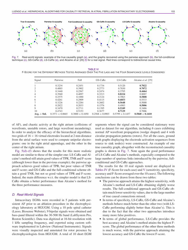
Fig. 7. Real-world signals: example of the true causality graph (a), and the graphs recovered using the pairwise approach (b), the full-conditionaltechnique (c), GS-CaRe (d), LS-CaRe (e), and Alcaine et al. [25] (f) for a real signal. Red lines correspond to bidirectional causal links.

TABLE IVF-SCORE FOR THE DIFFERENT METHODS TESTED AVERAGED OVER THE FIVE LAGS AND THE FOUR SIGNIFICANCE LEVELS CONSIDERED

Signal Pairwise Full GS-CaRe LS-CaRe Alcaine et al. [25]

1 0.3234 0.2451 0.1734 0.5120 0.70222 0.4003 0.3902 0.2773 0.7030 0.70723 0.3440 0.2567 0.2474 0.3795 0.44644 0.3940 0.4097 0.3213 0.8224 0.80075 0.2575 0.1890 0.2124 0.3963 0.58086 0.4261 0.2909 0.4115 0.6853 0.55337 0.3226 0.2284 0.2602 0.5648 0.50008 0.2822 0.2033 0.1576 0.4983 0.50069 0.3470 0.2711 0.1395 0.5249 0.348610 0.4743 0.5153 0.3677 0.7129 0.7006Avg. ± Std. 0.3571 ± 0.0665 0.3000 ± 0.1050 0.2568 ± 0.0903 0.5799 ± 0.1457 0.5840 ± 0.1410

of AF), and chaotic activity at the right atrium (collisions ofwavefronts, unstable rotors, and large wavefront meandering).In order to analyze the efficacy of the hierarchical algorithms,two grids of 16 × 16 virtual electrodes located at 2 mm distancefrom the atrial surface were used to compute unipolar electro-grams: one in the right atrial appendage, and the other in thecenter of the right atrium.

Fig. 5(d)–(f) shows that the results for this more realisticmodel are similar to those of the simpler one: LS-CaRe and Al-caine’s method still attain good values of TPR, TNR and F-score(although lower than in the previous example); the pairwise ap-proach achieves good values of TPR, but poor values of TNRand F-score; and GS-CaRe and the full-conditional scheme ob-tain a good TNR, but not so good values of TPR and F-score.Indeed, the main difference w.r.t. the simpler model is that LS-CaRe obtains a better performance than Alcaine’s method forthe three performance measures.

D. Real-World Signals

Intracavitary EGMs were recorded in 5 patients with per-sistent AF prior to an ablation procedure in the electrophysi-ology laboratory at HGUGM. Using a 10 pole spiral catheter(Lasso, Biosense Webster), 9 bipolar signals were obtained andbass-pand filtered within the 30-500 Hz band (LabSystem Pro,Boston Scientific). Data was digitized at 16-bit resolution with1 kHz sampling frequency, and exported using custom soft-ware implemented in Labview (National Instruments). Signalswere visually inspected and annotated for rotor presence byelectrophysiologists from HGUGM. A total of 10 short EGM

segments where the signal can be considered stationary wereused as dataset for our algorithm, including 6 cases exhibitingnormal AP wavefront propagation (wedge shaped) and 4 withcircular propagation patterns (rotors). For all the cases, groundtruth graphs displaying the electrode activation sequences fromsource to sink node(s) were constructed. An example of onetrue causality graph, altogether with the reconstructed causalitygraphs is shown in Fig. 7. Note again the good performanceof LS-CaRe and Alcaine’s methods, especially compared to thelarge number of spurious links introduced by the pairwise, full-conditional and GS-CaRe approaches.

The results for the 10 real signals tested are displayed inTables IV (F-Score for each case) and V (sensitivity, specificity,accuracy and F-Score averaged over the 10 cases). The followingconclusions can be drawn from these two tables:

� The pairwise approach attains the highest sensitivity, withAlcaine’s method and LS-CaRe obtaining slightly worseresults. The full-conditional approach and GS-CaRe ob-tain much lower sensitivity values, due to the large numberof true causal connections missed.

� In terms of specificity, LS-CaRe, GS-CaRe and Alcaine’smethods behave much better than the other two (with LS-CaRe performing slightly better than Alcaine’s). This isdue to the fact that the other two approaches introducemany more false positives.

� In terms of global performance, LS-CaRe provides thebest accuracy and Alcaine’s method attains the highest F-score. The global performance of the other three methodsis much worse, with the pairwise approach attaining thelowest accuracy and GS-CaRe the lowest F-score.


TABLE VAVERAGED RESULTS FOR SEVERAL PERFORMANCE METRICS, THE FIVE LAGS AND THE FOUR SIGNIFICANCE LEVELS CONSIDERED

Signal Pairwise Full GS-CaRe LS-CaRe Alcaine et al. [25]

Sensitivity 0.6607 ± 0.2062 0.4772 ± 0.1984 0.2439 ± 0.1026 0.6059 ± 0.1772 0.6110 ± 0.1333Specificity 0.7723 ± 0.0854 0.8152 ± 0.0750 0.9350 ± 0.0205 0.9508 ± 0.0162 0.9470 ± 0.0188Accuracy 0.7614 ± 0.0619 0.7819 ± 0.0597 0.8656 ± 0.0209 0.9162 ± 0.0250 0.9135 ± 0.0290F-Score 0.3571 ± 0.0665 0.3000 ± 0.1050 0.2568 ± 0.0903 0.5799 ± 0.1457 0.5840 ± 0.1410

V. CONCLUSION

A generic hierarchical framework and two specific algo-rithms for causality retrieval in intracavitary EGMs, based onG-causality, have been described in this paper. Both algorithmsrely on the initial discovery of the root node, but the influenceof this node on their performance is very different: GS-CaRedepends critically on a proper selection of this root node, sincea global search is then started from it and an erroneous choiceinvariably leads to poor results, whereas LS-CaRe only needsthis root node as the starting point for its local search and thus ismuch more robust w.r.t. an erroneous selection. This robustness,altogether with the reduced number of false alarms introducedby the local search, explains the much better performance of LS-CaRe, which shows a comparable performance to the methodproposed in [25] by Alcaine et al. Indeed, both LS-CaRe andAlcaine’s approach have the same goal: restricting the searchfor causal connections to neighbors. However, the proceduresfollowed to achieve this goal are very different: defining a novellocal propagation direction measure (Alcaine’s) and perform-ing a structured hierarchical search (LS-CaRe). From a clinicalpoint of view, the developed methods can be used by cardi-ologists for two purposes: (1) discriminating among differentpropagation patterns (e.g., flat or circular propagation vs. ro-tors); and (2) determining the direction of the received AP wave-front. In future work, we plan to incorporate other alternativemeasures of causality, like transfer entropy or the phase slopeindex, as well as Alcaine’s novel local propagation directionmeasure, into the flexible framework described here.

ACKNOWLEDGMENT

The authors would like to thank Dr. Angel Arenal, from Hos-pital General Universitario Gregorio Maranon, for providingaccess to the real data, annotations and expert clinical advice onelectrophysiology in general and AF in particular.

REFERENCES

[1] P. Kirchhof et al., “2016 ESC Guidelines for the managementof atrial fibrillation developed in collaboration with EACTS,” Eu-ropace, vol. 18, no. 11, pp. 1609–1678, 2016. [Online]. Available:http://www.ncbi.nlm.nih.gov/pubmed/27567465

[2] W. B. Kannel and E. J. Benjamin, “Status of the epidemiology of atrialfibrillation,” Med. Clinics North Amer., vol. 92, no. 1, pp. 17–40, 2008.

[3] L. Y. Chen, N. Sotoodehnia, P. Buzkova, F. Lopez, L. Yee, and S. Heckbert,“Atrial fibrillation and the risk of sudden cardiac death: The atherosclerosisrisk in communities study and cardiovascular health study,” JAMA InternalMed., vol. 173, no. 1, pp. 29–35, 2013.

[4] P. A. Wolf, R. D. Abbott, and W. B. Kannel, “Atrial fibrillation as anindependent risk factor for stroke: The Framingham study,” Stroke, vol. 22,pp. 983–988, 1991.

[5] S. Nattel, D. Li, and L. Yue, “Basic mechanisms of atrial fibrillation—very new insights into very old ideas,” Annu. Rev. Physiol., vol. 62, no. 1,pp. 51–77, Jan. 2000.

[6] D. E. Krummen and S. M. Narayan, “Mechanisms for the initiation ofhuman atrial fibrillation,” Heart Rhythm, vol. 6, no. 8, pp. S12–S16, Aug.2009.

[7] G. Moe, “On the multiple wavelet hypothesis of atrial fibrillation,” ArchInt. Phamacodyn Ther, no. 140, pp. 183–188, 1962.

[8] M. A. Allessie, W. Lammers, F. Bonke, and J. Hollen, “Experimentalevaluation of Moe’s wavelet hypothesis of atrial fibrillation,” in CardiacElectrophysiology and Arrhythmias, D. Zipes and J. Jalife, Eds. New York,NY, USA: Grune & Stratton, 1985, pp. 265–275.

[9] J. Jalife, O. Berenfeld, and M. Mansour, “Mother rotors and fibrilla-tory conduction: a mechanism of atrial fibrillation,” Cardiovascular Res.,vol. 54, no. 2, pp. 204–216, 2002.

[10] H. Calkins et al., “2012 HRS/EHRA/ECAS expert consensus statement oncatheter and surgical ablation of atrial fibrillation: recommendations forpatient selection, procedural techniques, patient management and follow-up, definitions, endpoints, and research trial design,” Heart Rhythm, vol. 9,no. 4, pp. 632–696.e21, 2012.

[11] K. Nademanee et al., “A new approach for catheter ablation of atrialfibrillation: Mapping of the electrophysiologic substrate,” J. Amer. Col-lege Cardiol., vol. 43, no. 11, pp. 2044–53, 2004. [Online]. Available:http://www.ncbi.nlm.nih.gov/pubmed/15172410

[12] J. Ng and J. J. Goldberger, “Understanding and interpreting domi-nant frequency analysis of AF electrograms,” J. Cardiovascular Elec-trophysiol., vol. 18, no. 6, pp. 680–685, 2007. [Online]. Available:http://doi.wiley.com/10.1111/j.1540-8167.2007.00832.x

[13] Y. Takahashi et al., “Organization of frequency spectra of atrial fibrilla-tion: Relevance to radiofrequency catheter ablation,” J. CardiovascularElectrophysiol., vol. 17, no. 4, pp. 382–388, 2006.

[14] G. W. Botteron and J. M. Smith, “A technique for measurement of theextent of spatial organization of atrial activation during atrial fibrillationin the intact human heart,” IEEE Trans. Biomed. Eng., vol. 42, no. 6,pp. 579–586, Jun. 1995.

[15] S. L. Bressler and A. K. Seth, “Wiener–Granger causality: A well estab-lished methodology,” NeuroImage, vol. 58, no. 2, pp. 323–329, 2011.

[16] L. Faes, A. Porta, and G. Nollo, “Testing frequency-domain causalityin multivariate time series,” IEEE Trans. Biomed. Eng., vol. 57, no. 8,pp. 1897–1906, Aug. 2010.

[17] S. Kleinberg and G. Hripcsak, “A review of causal inference for biomed-ical informatics,” J. Biomed. Informat., vol. 44, no. 6, pp. 1102–1112,2011.

[18] L. Faes and G. Nollo, “Assessing frequency domain causality in cardio-vascular time series with instantaneous interactions,” Methods Inf. Med.,vol. 49, no. 5, p. 453, 2010.

[19] A. Porta, T. Bassani, V. Bari, and S. Guzzetti, “Granger causality in cardio-vascular variability series: Comparison between model-based and model-free approaches,” in Proc. IEEE Eng. Med. Biol. Conf., 2012, pp. 3684–3687.

[20] U. Richter et al., “A novel approach to propagation pattern analysis inintracardiac atrial fibrillation signals,” Ann. Biomed. Eng., vol. 39, no. 1,pp. 310–323, 2011.

[21] U. Richter, L. Faes, F. Ravelli, and L. Sornmo, “Propagation pattern anal-ysis during atrial fibrillation based on sparse modeling,” IEEE Trans.Biomed. Eng., vol. 59, no. 5, pp. 1319–1328, May 2012.

[22] M. Rodrigo, A. Liberos, M. Guillem, J. Millet, and A. M. Climent,“Causality relation map: a novel methodology for the identification ofhierarchical fibrillatory processes,” in Proc. Comput. Cardiol, Sep. 2011,pp. 173–176.

[23] M. Rodrigo, M. S. Guillem, A. Liberos, J. Millet, O. Berenfeld, and A.M. Climent, “Identification of fibrillatory sources by measuring causalrelationships,” in Proc. Comput. Cardiol., Sep. 2012, pp. 705–708.


[24] M. Rodrigo et al., “Identification of dominant excitation patterns andsources of atrial fibrillation by causality analysis,” Ann. Biomed. Eng.,vol. 44, no. 8, pp. 2364–2376, Aug. 2016.

[25] A. Alcaine et al., “A multi-variate predictability framework to assessinvasive cardiac activity and interactions during atrial fibrillation,” IEEETrans. Biomed. Eng., vol. 64, no. 5, pp. 1157–1168, May 2017.

[26] D. Luengo, G. Rıos-Munoz, and V. Elvira, “Causality analysis of atrialfibrillation electrograms,” in Proc. Comput. Cardiol., 2015, pp. 585–588.

[27] D. Luengo, G. Rıos-Munoz, V. Elvira, and A. Artes-Rodrıguez, “A hierar-chical algorithm for causality discovery among atrial fibrillation electro-grams,” in Proc. IEEE Int. Conf. Acoust., Speech Signal Process., 2016,pp. 774–778.

[28] C. W. J. Granger, “Investigating causal relations by econometric modelsand cross-spectral methods,” Econometrica, vol. 37, pp. 424–438, 1969.

[29] P. Stoica and Y. Selen, “Model-order selection: A review of informationcriterion rules,” IEEE Signal Process. Mag., vol. 21, no. 4, pp. 36–47, Jul.2004.

[30] J. Geweke, “Measures of conditional linear dependence and feedbackbetween time series,” J. Amer. Stat. Assoc., vol. 79, pp. 907–915, 1984.

[31] J. D. Gibbons and J. W. Pratt, “p-values: interpretation and methodology,”Amer. Stat., vol. 29, no. 1, pp. 20–25, 1975.

[32] M. E. Masson, “A tutorial on a practical Bayesian alternative to null-hypothesis significance testing,” Behav. Res. Methods, vol. 43, no. 3,pp. 679–690, 2011.

[33] J. Keener and J. Sneyd, Mathematical Physiology I: Cellular Physiology.New York, NY, USA: Springer, 2010.

[34] A. K. Seth, “A MATLAB toolbox for Granger causal connectivity analy-sis,” J. Neurosci. Methods, vol. 186, no. 2, pp. 262–273, 2010.

[35] D. Crisan, J. Miguez, and G. Rios, “A simple scheme for the paral-lelization of particle filters and its application to the tracking of complexstochastic systems,” Tech. Rep. arXiv:1407.8071, 2014. [Online]. Avail-able: https://arxiv.org/abs/1407.8071

[36] J. Keener and J. Sneyd, Mathematical Physiology II: Systems Physiology.New York, NY, USA: Springer, 2010.

[37] C. Pantaleon, D. Luengo, and I. Santamarıa, “Optimal estimation ofchaotic signals generated by piecewise-linear maps,” IEEE Signal Pro-cess. Lett., vol. 7, no. 8, pp. 235–237, Aug. 2000.

[38] D. Luengo, I. Santamarıa, and L. Vielva, “A general solution to blindinverse problems for sparse input signals,” Neurocomputing, vol. 69, no. 1,pp. 198–215, 2005.

[39] V. Elvira, L. Martino, D. Luengo, and M. F. Bugallo, “Improving popula-tion Monte Carlo: Alternative weighting and resampling schemes,” SignalProcess., vol. 131, pp. 77–91, 2017.

[40] G. Seemann, C. Hoper, F. B. Sachse, O. Dossel, A. V. Holden, and H.Zhang, “Heterogeneous three-dimensional anatomical and electrophysi-ological model of human atria,” Philosoph. Trans. Roy. Soc. London A,Math., Phys. Eng. Sci., vol. 364, no. 1843, pp. 1465–1481, 2006.

[41] C. Sanchez, A. Bueno-Orovio, E. Pueyo, and B. Rodrıguez, “Atrial fib-rillation dynamics and ionic block effects in six heterogeneous human3D virtual atria with distinct repolarization dynamics,” Frontiers Bioeng.Biotechnol,, vol. 5, pp. 1–13, May 2017.

[42] M. M. Maleckar, J. L. Greenstein, W. R. Giles, and N. A. Trayanova, “K+current changes account for the rate dependence of the action potentialin the human atrial myocyte,” AJP, Heart Circulatory Physiol., vol. 297,no. 4, pp. H1398–H1410, 2009.

[43] E. A. Heidenreich, J. M. Ferrero, M. Doblare, and J. F. Rodrıguez, “Adap-tive macro finite elements for the numerical solution of monodomainequations in cardiac electrophysiology,” Ann. Biomed. Eng., vol. 38, no. 7,pp. 2331–2345, 2010.

hierarchical algorithms for causality retrieval in atrial...

Documents