Hierarchical adaptive low-rank format with applications todiscretized PDEs

Stefano Massei

Joint work with D. Kressner (EPFL) and L. Robol (University of Pisa)

s.massei@tue.nl

Conference on Fast Direct Solvers, 23 October 2021

1 / 18

Sylvester equations coming from PDEs

We consider time-dependent PDEs of the form∂u∂t = Lu + f (u,∇u) t ∈ [0,Tmax]u(x , y , 0) = u0(x , y) (x , y) ∈ Ω := [a, b]× [c, d ]B.C. (x , y) ∈ ∂Ω and t > 0

,

where L = Lx + Ly is elliptic with a Kronecker sum structured discretization [1,2]L := I ⊗ A + B ⊗ I, and f is nonlinear.

Applying the IMEX Euler approach, where L is treated implicitly, yields [3]

(I −∆t · L)ut+1 = ut + ∆t(f (ut ,∇ut) + B.C .),

i.e., an iterative scheme where at each step we need to solve a Sylvester equation.

Challenge: Can we go large-scale?

[1] Townsend, Olver. The automatic solution of partial differential equations using a global spectral method. Journal of Computational Physics, 2015.[2] Palitta, Simoncini. Matrix-equation-based strategies for convection–diffusion equations. BIT, 2016.[3] D’Autilia, Sgura, Simoncini. Matrix-oriented discretization methods for reaction-diffusion PDEs: Comparisons and applications. Computers &Mathematics with Applications, 2020.

2 / 18

Main topic of the talk

We have an integration scheme that requires solving a sequence of Sylvester eqns:

AXt + XtB = Ct .

Ideal situation: Xt is low-rank ∀t Efficient storage and computation of Xt .

When the solution u(·, ·, t) is smooth, Xt is (numerically) low-rank,The presence of isolated singularities makes Xt only locally low-rank.Singularities that move during the time evolution time-dependent localstructure.

Question: Can we fully exploit local and time-dependent structures in the timeintegration?

3 / 18

Main topic of the talk

We have an integration scheme that requires solving a sequence of Sylvester eqns:

AXt + XtB = Ct .

Ideal situation: Xt is low-rank ∀t Efficient storage and computation of Xt .

When the solution u(·, ·, t) is smooth, Xt is (numerically) low-rank,The presence of isolated singularities makes Xt only locally low-rank.Singularities that move during the time evolution time-dependent localstructure.

Question: Can we fully exploit local and time-dependent structures in the timeintegration?

3 / 18

Burgers equation

As running example, consider the 2D Burgers equation:∂u∂t = 10−3

(∂2u∂x2 + ∂2u

∂y2

)− u ·

(∂u∂x + ∂u

∂y

)u(x , y , t) = 1

1+exp(103(x+y−t)/2) t = 0 or (x , y) ∈ ∂Ω

4 / 18

Burgers equation

As running example, consider the 2D Burgers equation:∂u∂t = 10−3

(∂2u∂x2 + ∂2u

∂y2

)− u ·

(∂u∂x + ∂u

∂y

)u(x , y , t) = 1

1+exp(103(x+y−t)/2) t = 0 or (x , y) ∈ ∂Ω

Blue blocks: Full rank submatrices, Grey blocks: Low-rank submatrices4 / 18

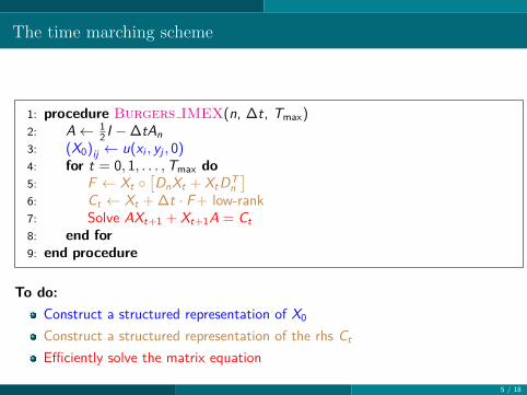
The time marching scheme

1: procedure Burgers IMEX(n, ∆t, Tmax)2: A← 1

2 I −∆tAn3: (X0)ij ← u(xi , yj , 0)4: for t = 0, 1, . . . ,Tmax do5: F ← Xt

[DnXt + XtDT

n]

6: Ct ← Xt + ∆t · F + low-rank7: Solve AXt+1 + Xt+1A = Ct8: end for9: end procedure

An = n × n discretized second derivative operator,Dn = n × n discretized first derivative operator.

5 / 18

The time marching scheme

1: procedure Burgers IMEX(n, ∆t, Tmax)2: A← 1

2 I −∆tAn3: (X0)ij ← u(xi , yj , 0)4: for t = 0, 1, . . . ,Tmax do5: F ← Xt

[DnXt + XtDT

n]

6: Ct ← Xt + ∆t · F + low-rank7: Solve AXt+1 + Xt+1A = Ct8: end for9: end procedure

To do:Construct a structured representation of X0

Construct a structured representation of the rhs Ct

Efficiently solve the matrix equation

5 / 18

Finding a low-rank block representation

Given M ∈ Rn×n, ε > 0, maxrank ∈ N and let LRA(M, ε,maxrank) be such that

LRA(M, ε,maxrank)M such that ‖M − M‖ ≤ ε, rank(M) ≤ maxrank X

failure 7

Example: LRA = maxrank iterations of the Adaptive Cross Approximationalgorithm.

M =

LRALRA 7

LRA LRA

LRA LRA

LRA X LRA X

LRA 7 LRA XLRA LRA

LRA LRA

12 9

11

7 X

X 7

10

11

LRA

LRA

LRA

LRA

LRA

LRA

LRA

LRA

7XX7

7XX7

1211

1013

6 / 18

Finding a low-rank block representation

Given M ∈ Rn×n, ε > 0, maxrank ∈ N and let LRA(M, ε,maxrank) be such that

LRA(M, ε,maxrank)M such that ‖M − M‖ ≤ ε, rank(M) ≤ maxrank X

failure 7

Example: LRA = maxrank iterations of the Adaptive Cross Approximationalgorithm.

M = LRA

LRA 7

LRA LRA

LRA LRA

LRA X LRA X

LRA 7 LRA XLRA LRA

LRA LRA

12 9

11

7 X

X 7

10

11

LRA

LRA

LRA

LRA

LRA

LRA

LRA

LRA

7XX7

7XX7

1211

1013

6 / 18

Finding a low-rank block representation

Given M ∈ Rn×n, ε > 0, maxrank ∈ N and let LRA(M, ε,maxrank) be such that

LRA(M, ε,maxrank)M such that ‖M − M‖ ≤ ε, rank(M) ≤ maxrank X

failure 7

Example: LRA = maxrank iterations of the Adaptive Cross Approximationalgorithm.

M =

LRA

LRA 7

LRA LRA

LRA LRA

LRA X LRA X

LRA 7 LRA XLRA LRA

LRA LRA

12 9

11

7 X

X 7

10

11

LRA

LRA

LRA

LRA

LRA

LRA

LRA

LRA

7XX7

7XX7

1211

1013

6 / 18

Finding a low-rank block representation

Given M ∈ Rn×n, ε > 0, maxrank ∈ N and let LRA(M, ε,maxrank) be such that

LRA(M, ε,maxrank)M such that ‖M − M‖ ≤ ε, rank(M) ≤ maxrank X

failure 7

Example: LRA = maxrank iterations of the Adaptive Cross Approximationalgorithm.

M =

LRALRA 7

LRA LRA

LRA LRA

LRA X LRA X

LRA 7 LRA XLRA LRA

LRA LRA

12 9

11

7 X

X 7

10

11

LRA

LRA

LRA

LRA

LRA

LRA

LRA

LRA

7XX7

7XX7

1211

1013

6 / 18

Finding a low-rank block representation

Given M ∈ Rn×n, ε > 0, maxrank ∈ N and let LRA(M, ε,maxrank) be such that

LRA(M, ε,maxrank)M such that ‖M − M‖ ≤ ε, rank(M) ≤ maxrank X

failure 7

Example: LRA = maxrank iterations of the Adaptive Cross Approximationalgorithm.

M =

LRALRA 7

LRA LRA

LRA LRA

LRA X LRA X

LRA 7 LRA X

LRA LRA

LRA LRA

12 9

11

7 X

X 7

10

11

LRA

LRA

LRA

LRA

LRA

LRA

LRA

LRA

7XX7

7XX7

1211

1013

6 / 18

Finding a low-rank block representation

Given M ∈ Rn×n, ε > 0, maxrank ∈ N and let LRA(M, ε,maxrank) be such that

LRA(M, ε,maxrank)M such that ‖M − M‖ ≤ ε, rank(M) ≤ maxrank X

failure 7

Example: LRA = maxrank iterations of the Adaptive Cross Approximationalgorithm.

M =

LRALRA 7

LRA LRA

LRA LRA

LRA X LRA X

LRA 7 LRA X

LRA LRA

LRA LRA

12 9

11

7 X

X 7

10

11

LRA

LRA

LRA

LRA

LRA

LRA

LRA

LRA

7XX7

7XX7

1211

1013

6 / 18

Finding a low-rank block representation

Given M ∈ Rn×n, ε > 0, maxrank ∈ N and let LRA(M, ε,maxrank) be such that

LRA(M, ε,maxrank)M such that ‖M − M‖ ≤ ε, rank(M) ≤ maxrank X

failure 7

Example: LRA = maxrank iterations of the Adaptive Cross Approximationalgorithm.

M =

LRALRA 7

LRA LRA

LRA LRA

LRA X LRA X

LRA 7 LRA XLRA LRA

LRA LRA

12 9

117 X

X 7

10

11

LRA

LRA

LRA

LRA

LRA

LRA

LRA

LRA

7XX7

7XX7

1211

1013

6 / 18

Finding a low-rank block representation

Given M ∈ Rn×n, ε > 0, maxrank ∈ N and let LRA(M, ε,maxrank) be such that

LRA(M, ε,maxrank)M such that ‖M − M‖ ≤ ε, rank(M) ≤ maxrank X

failure 7

Example: LRA = maxrank iterations of the Adaptive Cross Approximationalgorithm.

M =

LRALRA 7

LRA LRA

LRA LRA

LRA X LRA X

LRA 7 LRA XLRA LRA

LRA LRA

12 9

11

7 X

X 7

10

11

LRA

LRA

LRA

LRA

LRA

LRA

LRA

LRA

7XX7

7XX7

1211

1013

6 / 18

Finding a low-rank block representation

Given M ∈ Rn×n, ε > 0, maxrank ∈ N and let LRA(M, ε,maxrank) be such that

LRA(M, ε,maxrank)M such that ‖M − M‖ ≤ ε, rank(M) ≤ maxrank X

failure 7

Example: LRA = maxrank iterations of the Adaptive Cross Approximationalgorithm.

M =

LRALRA 7

LRA LRA

LRA LRA

LRA X LRA X

LRA 7 LRA XLRA LRA

LRA LRA

12 9

11

7 X

X 7

10

11

LRA

LRA

LRA

LRA

LRA

LRA

LRA

LRA

7XX7

7XX7

1211

1013

6 / 18

Finding a low-rank block representation

Given M ∈ Rn×n, ε > 0, maxrank ∈ N and let LRA(M, ε,maxrank) be such that

LRA(M, ε,maxrank)M such that ‖M − M‖ ≤ ε, rank(M) ≤ maxrank X

failure 7

Example: LRA = maxrank iterations of the Adaptive Cross Approximationalgorithm.

M =

LRALRA 7

LRA LRA

LRA LRA

LRA X LRA X

LRA 7 LRA XLRA LRA

LRA LRA

12 9

11

7 X

X 7

10

11

LRA

LRA

LRA

LRA

LRA

LRA

LRA

LRA

7XX7

7XX7

1211

1013

6 / 18

Hierarchically Adaptive Low-Rank matrices (HALR)

We can associate with M the quad-tree cluster T of the form:J1, nK×J1, nK

J1, n2

K×J1, n2

K J1, n2

K×J n2

, nK J n2

, nK×J1, n2

K J n2

, nK×J n2

, nKlow-rank low-rank low-rank

J1, n4

K×J1, n4

K J1, n4

K×J n4

, n2

K J n4

, n2

K×J1, n4

K J n4

, n2

K×J n4

, n2

Klow-rank low-rank

J n4

, 38nK×J1, n

8K J n

4, 38nK×J n

8, n

4K J 3

4n, n

2K×J1, n

8K J 3

4n, n

2K×J n

8, n

4K

low-rank dense dense low-rank

J n8

, n4

K×J 34n, n

2KJ n

8, n

4K×J n

4, 34nKJ1, n

8, K×J n

4, 34nKJ1, n

8K×J n

4, 34nK

low-rank dense dense low-rank

Def: M ∈ Rn×n is (T , r)-HALR if its submatrices corresponding to the low-rankleaves of T have rank ≤ r .

What we can do with the HALR format:Matrix operations between HALR matrices with different partitioningsComplexity is log/log2-proportional to the storage cost of the outcomeAdjust/Refine the cluster (in the spirit of the construction algorithm)

7 / 18

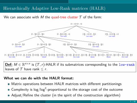
Hierarchically Adaptive Low-Rank matrices (HALR)

We can associate with M the quad-tree cluster T of the form:J1, nK×J1, nK

J1, n2

K×J1, n2

K J1, n2

K×J n2

, nK J n2

, nK×J1, n2

K J n2

, nK×J n2

, nKlow-rank low-rank low-rank

J1, n4

K×J1, n4

K J1, n4

K×J n4

, n2

K J n4

, n2

K×J1, n4

K J n4

, n2

K×J n4

, n2

Klow-rank low-rank

J n4

, 38nK×J1, n

8K J n

4, 38nK×J n

8, n

4K J 3

4n, n

2K×J1, n

8K J 3

4n, n

2K×J n

8, n

4K

low-rank dense dense low-rank

J n8

, n4

K×J 34n, n

2KJ n

8, n

4K×J n

4, 34nKJ1, n

8, K×J n

4, 34nKJ1, n

8K×J n

4, 34nK

low-rank dense dense low-rank

Def: M ∈ Rn×n is (T , r)-HALR if its submatrices corresponding to the low-rankleaves of T have rank ≤ r .

What we can do with the HALR format:Matrix operations between HALR matrices with different partitioningsComplexity is log/log2-proportional to the storage cost of the outcomeAdjust/Refine the cluster (in the spirit of the construction algorithm)

7 / 18

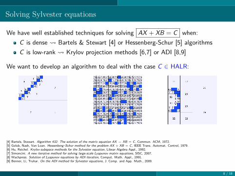
Solving Sylvester equations

We have well established techniques for solving AX + XB = C when:C is dense Bartels & Stewart [4] or Hessenberg-Schur [5] algorithmsC is low-rank Krylov projection methods [6,7] or ADI [8,9]

We want to develop an algorithm to deal with the case C ∈ HALR:

[4] Bartels, Stewart. Algorithm 432: The solution of the matrix equation AX − XB = C , Commun. ACM, 1972.[5] Golub, Nash, Van Loan. Hessenberg–Schur method for the problem AX + XB = C , IEEE Trans. Automat. Control, 1979.[6] Hu, Reichel. Krylov-subspace methods for the Sylvester equation, Libear Algebra Appl., 1992.[7] Simoncini. A new iterative method for solving large-scale Lyapunov matrix equations, SISC, 2007.[8] Wachpress. Solution of Lyapunov equations by ADI iteration, Comput. Math. Appl., 1991.[9] Benner, Li, Truhar. On the ADI method for Sylvester equations, J. Comp. and App. Math., 2009.

8 / 18

Solving Sylvester equations

We have well established techniques for solving AX + XB = C when:C is dense Bartels & Stewart [4] or Hessenberg-Schur [5] algorithmsC is low-rank Krylov projection methods [6,7] or ADI [8,9]

We want to develop an algorithm to deal with the case C ∈ HALR:

[4] Bartels, Stewart. Algorithm 432: The solution of the matrix equation AX − XB = C , Commun. ACM, 1972.[5] Golub, Nash, Van Loan. Hessenberg–Schur method for the problem AX + XB = C , IEEE Trans. Automat. Control, 1979.[6] Hu, Reichel. Krylov-subspace methods for the Sylvester equation, Libear Algebra Appl., 1992.[7] Simoncini. A new iterative method for solving large-scale Lyapunov matrix equations, SISC, 2007.[8] Wachpress. Solution of Lyapunov equations by ADI iteration, Comput. Math. Appl., 1991.[9] Benner, Li, Truhar. On the ADI method for Sylvester equations, J. Comp. and App. Math., 2009.

8 / 18

Hierarchical low-rank structure in A, B

The matrices A and B are usually banded or have low-rank off-diagonal blocks.

From now on we assume that A and B can be block partitioned as:

A =[A11 A12A21 A22

]=[A11

A22

]︸ ︷︷ ︸

Block structured

+[

A12A21

]︸ ︷︷ ︸

low-rank

.

Simple idea: store low-rank blocks as outer products, and diagonal onesrecursively (H-matrices, HODLR) [10].

[10] Hackbusch. Hierarchical Matrices: Algorithms and Analysis, Springer Series in Computational Mathematics, 2015.

9 / 18

Hierarchical low-rank structure in A, B

The matrices A and B are usually banded or have low-rank off-diagonal blocks.

From now on we assume that A and B can be block partitioned as:

A =[A11 A12A21 A22

]=[A11

A22

]︸ ︷︷ ︸

Block structured

+[

A12A21

]︸ ︷︷ ︸

low-rank

.

Simple idea: store low-rank blocks as outer products, and diagonal onesrecursively (H-matrices, HODLR) [10].

[10] Hackbusch. Hierarchical Matrices: Algorithms and Analysis, Springer Series in Computational Mathematics, 2015.

9 / 18

Sylvester equations with A, B ∈ HODLR and C ∈ HALR

Idea: HODLR matrices can be block-diagonalized via low-rank modifications.

Splitting A and B into their block diagonal and antidiagonal parts, leads to:

Solve the equation[A11

A22

]X0 + X0

[B11

B22

]=[C11 C12C21 C22

],

Update X0 by solving [11]

A δX + δX B = −[

A12A21

]X0 − X0

[B12

B21

]︸ ︷︷ ︸

low-rank

.

The first equation can be decomposed in 4 equations with HODLR coefficients ofdimension n

2 . This leads to a divide-and-conquer scheme.

[11] Kressner, Massei, Robol. Low-rank updates and a divide-and-conquer algorithm for linear matrix equations, SISC, 2019.

10 / 18

Sylvester equations with A, B ∈ HODLR and C ∈ HALR (cont’d)

1: procedure D&C Sylv(A,B,C)2: if A,B are small matrices then return Bartels&Stewart(A,B,C)3: end if4: if C = CLC∗

R is low-rank then return low rank Sylv(A,B,CL,CR )5: end if6: Decompose

A =[A11 0

0 A22

]+ δA, B =

[B11 0

0 B22

]+ δB, C =

[C11 C12C21 C22

]7: X11 ← D&C Sylv(A11,B11,C11), X12 ← D&C Sylv(A11,B22,C12)8: X21 ← D&C Sylv(A22,B11,C21), X22 ← D&C Sylv(A22,B22,C22)

9: X0 ←[X11 X12X21 X22

]10: Compute CL and CR such that CLC∗

R = −δAX0 − X0δB11: δX ← low rank Sylv(A,B,CL,CR )12: return X0 + δX13: end procedure

11 / 18

Complexity and solution structure of D&C

AX + XB = C

Assumptions:

C has low-rank blocks of rank ≤ r ; the storage cost of C is O(S)A and B are HODLR matrices with HODLR rank ≤ kBartels&Stewart is applied only on matrices of size ≤ nmin

Solving equations with low-rank RHS costs O(k2n log2(n))

TheoremThe solution X has the same HALR structure of C with ranks O(r + k log(n))and the D&C method costs O(S · k2 log2(n)).

Remark: The estimate O(r + k log(n)) for the ranks in X is typically pessimistic.

12 / 18

Numerical results: Burgers equation

∂u∂t = 10−3

(∂2u∂x2 + ∂2u

∂y2

)− u ·

(∂u∂x + ∂u

∂y

)u(x , y , t) = 1

1+exp(103(x+y−t)/2) t = 0 or (x , y) ∈ ∂Ω

13 / 18

Numerical results: Burgers equation (cont’d)

10−1

100

101

n = 4096

10−1

100

101

n = 8192

Tim

epe

rite

ratio

n(s

)

0 1,000 2,000 3,000 4,000 5,000 6,000 7,000 8,00010−1

100

101

n = 16384

Iterations

low-rankHALR

Figure: 8000 Iteration timings of the Euler-IMEX scheme on Burgers equation fordifferent spatial discretization steps and maxrank = 50.

14 / 18

Allen-Cahn equation

∂u∂t − 5 · 10−5∆u = u(u − 1

2 )(1− u)u(x , y , 0) = 1

2 + 12 randn

∂u∂~n = 0 (x , y) ∈ ∂Ω

t = 0.3 t = 0.5 t = 18.0 t = 35.0

15 / 18

Allen-Cahn equation (cont’d)

100

102 n = 4096

100

102 n = 8192

Tim

epe

rite

ratio

n(s

)

50 100 150 200 250 300 350 400

100

102 n = 16384

Iterations

low-rankHALRDense

Figure: 400 Iteration timings of the Euler-IMEX scheme on Allen-Cahn equation fordifferent spatial discretization steps and maxrank = 100

16 / 18

Comparison with FFT-based solvers

HALR-based algorithms

Burgers Allen-Cahnn Ttot (s) Avg. Tlyap (s) Ttot (s) Avg. Tlyap (s)

4096 22334.0 1.32 505.2 0.818192 57096.9 4.01 1147.4 1.82

16384 119130.4 9.55 2336.8 3.32

FFT-based algorithms

Burgers Allen-Cahnn Ttot (s) Avg. Tlyap (s) Ttot (s) Avg. Tlyap (s)

4096 18094 2.26 174.97 0.448192 70541 8.82 847.3 2.12

16384 295507 36.94 2967 7.42

17 / 18

Conclusions & outlook

Take away messages:

Exploiting local and time-dependent structures can make the difference.Sylvester equations with HODLR coefficients A,B can be solved with acomplexity log2-proportional to the storage cost for the RHS.

What’s next?Can we deal with 3D problems? Which tensorial format is the most suitable?

Full story:S.M., L. Robol, D. Kressner. Hierarchical adaptive low-rank format withapplications to discretized PDEs, arXiv 2021.

18 / 18