heuristics for domain-independent planning 1....
TRANSCRIPT

Heuristics for Domain-Independent Planning
1. Introduction
Emil Keyder Silvia Richter
ICAPS 2011 Summer School on Automated Planning and Scheduling
June 2011
Emil Keyder, Silvia Richter Heuristics: 1. Introduction June 2011 1 / 24
Planning as Search
Heuristics
Problem Representation
Emil Keyder, Silvia Richter Heuristics: 1. Introduction June 2011 2 / 24
Contents
1. Introduction
2. Delete Relaxation Heuristics
3. Critical Path Heuristics
4. Context-Enhanced Additive Heuristic
5. Landmark Heuristics
6. Abstraction Heuristics
7. Final Comments
We try to give a general overview with the basic ideas and intuitions fordifferent heuristics
See references for details
Emil Keyder, Silvia Richter Heuristics: 1. Introduction June 2011 3 / 24
Planning as Search
Planning as Heuristic Search
Successful and robust
� Top four planners in the satisficing track of IPC6
� Several top planners in the optimal track
� Many well-performing planners from previous competitions
Standardized framework
� Mix and match heuristics and search techniques
Emil Keyder, Silvia Richter Heuristics: 1. Introduction June 2011 4 / 24
Planning as Search
Heuristic Search Planning
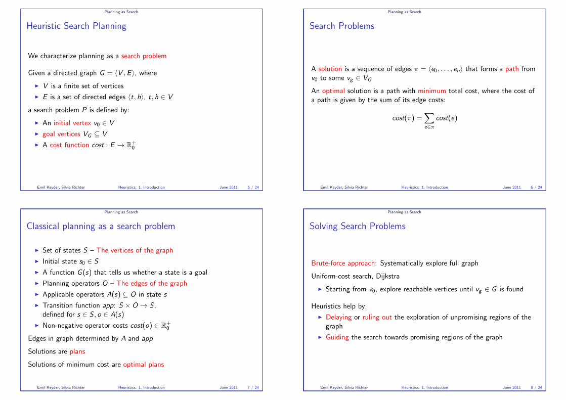
We characterize planning as a search problem
Given a directed graph G = �V ,E �, where� V is a finite set of vertices
� E is a set of directed edges �t, h�, t, h ∈ V
a search problem P is defined by:
� An initial vertex v0 ∈ V
� goal vertices VG ⊆ V
� A cost function cost : E → R+
0
Emil Keyder, Silvia Richter Heuristics: 1. Introduction June 2011 5 / 24
Planning as Search
Search Problems
A solution is a sequence of edges π = �e0, . . . , en� that forms a path fromv0 to some vg ∈ VG
An optimal solution is a path with minimum total cost, where the cost ofa path is given by the sum of its edge costs:
cost(π) =�
e∈πcost(e)
Emil Keyder, Silvia Richter Heuristics: 1. Introduction June 2011 6 / 24
Planning as Search
Classical planning as a search problem
� Set of states S – The vertices of the graph
� Initial state s0 ∈ S
� A function G (s) that tells us whether a state is a goal
� Planning operators O – The edges of the graph
� Applicable operators A(s) ⊆ O in state s
� Transition function app: S × O → S ,defined for s ∈ S , o ∈ A(s)
� Non-negative operator costs cost(o) ∈ R+
0
Edges in graph determined by A and app
Solutions are plans
Solutions of minimum cost are optimal plans
Emil Keyder, Silvia Richter Heuristics: 1. Introduction June 2011 7 / 24
Planning as Search
Solving Search Problems
Brute-force approach: Systematically explore full graph
Uniform-cost search, Dijkstra
� Starting from v0, explore reachable vertices until vg ∈ G is found
Heuristics help by:
� Delaying or ruling out the exploration of unpromising regions of thegraph
� Guiding the search towards promising regions of the graph
Emil Keyder, Silvia Richter Heuristics: 1. Introduction June 2011 8 / 24

Heuristics
Heuristics: What are they?
Heuristics are functions h : V �→ R+
0that estimate cost of path to a goal
node
Definition
h∗(v) is the cost of the lowest-cost path from v to some v � ∈ VG
h∗(v) → optimal solution in linear time� Intractable to compute in general, but useful comparison point
Objective : get as close as possible to h∗
Emil Keyder, Silvia Richter Heuristics: 1. Introduction June 2011 9 / 24
Heuristics
Heuristics: Admissibility
Definition
A heuristic h is admissible if for all s ∈ S : h(s) ≤ h∗(s)
Intuition: Heuristic is optimistic
� Never overestimates
Among admissible estimates h1 h2, the higher the better
� h∗ is an upper bound, so larger estimates are more exact
� A∗ expands fewer nodes when using higher admissible estimates1
1almost always, caveats applyEmil Keyder, Silvia Richter Heuristics: 1. Introduction June 2011 10 / 24
Heuristics
Maximum of Admissible Heuristics
Maximum of admissible heuristics
Let h1, h2 be two admissible heuristics. Note that
h1(s) ≤ h∗(s) ∧ h2(s) ≤ h∗(s) =⇒ max(h1(s), h2(s)) ≤ h∗(s)
The maximum of two admissible heuristics is amore informed admissible heuristic
Emil Keyder, Silvia Richter Heuristics: 1. Introduction June 2011 11 / 24
Heuristics
Sum of Admissible Heuristics
Sum of two admissible heuristics not in general admissible� h∗ + h∗ > h∗
But, consider two admissible estimates for length of ICAPS:
� h1: ≥ 2 days, because the workshops last 2 days
� h2: ≥ 3 days, because the main conference lasts 3 days
� We can infer that ICAPS lasts ≥ 5 days
Why? No “overlap” between the estimates.
Under certain conditions, the sum of two admissible heuristicsis an admissible heuristic
We say that a set H of such heuristics is additive
Emil Keyder, Silvia Richter Heuristics: 1. Introduction June 2011 12 / 24

Heuristics
Additive Admissible Heuristics: Action Partitioning
Simple criterion for admissible additivity: Count cost of each action in atmost one heuristic.
Given a task Π and a set of operators Oi ⊆ O, define the problem ΠOi
that is identical except
cost�(o) =
�cost(o) if o ∈ Oi
0 if o �∈ Oi
Action partitioning
An action partitioning is a set of problems ΠO1, . . . ,ΠOn
resulting from apartitioning of the actions O of a planning task into disjoint setsO1, . . . ,On.
Emil Keyder, Silvia Richter Heuristics: 1. Introduction June 2011 13 / 24
Heuristics
Additive Admissible Heuristics: Action Partitioning
Additivity of action partitioning
Let Π1, . . . ,Πn be an action partitioning and let hΠibe an admissible
estimate of the cost of Πi . Then the sum of the heuristics hΠiis
admissible:
n�
i=0
hΠi(s) ≤ h∗(s)
Proof sketch
Optimal plan for Π is also plan for each ΠOi, and the summed cost of
these plans is h∗. Admissible estimates must therefore sum to less than h∗.
Emil Keyder, Silvia Richter Heuristics: 1. Introduction June 2011 14 / 24
Heuristics
Additive Admissible Heuristics: Cost Partitioning
Action partitioning assigns the full cost of each operator to one problem,and zero to the others
Instead, distribute the cost of each action among different problems� Ensure total across problems sums to at most cost of action
Cost partitioning
A cost partitioning of Π is a set of problems Π0, . . . ,Πn that differ from Πonly in operator costs, that satisfy
n�
i=0
costi (o) ≤ cost(o)
where costi (o) is the cost of o in Πi ,
Emil Keyder, Silvia Richter Heuristics: 1. Introduction June 2011 15 / 24
Heuristics
Additive Admissible Heuristics: Cost Partitioning
Additivity of cost partitioning
Let Π0, . . . ,Πn be a cost partitioning of Π and let hΠ0, . . . , hΠn
beadmissible estimates for the costs of Π0, . . . ,Πn. Then the sum of theheuristics hΠi
is admissible:
n�
i=0
hΠi(s) ≤ h∗(s)
Proof sketch
Optimal plan for Π is also plan for each ΠOi, and the summed cost of
these plans is h∗. Admissible estimates must therefore sum to less than h∗.
Emil Keyder, Silvia Richter Heuristics: 1. Introduction June 2011 16 / 24
Heuristics
Heuristics: Consistency
Definition
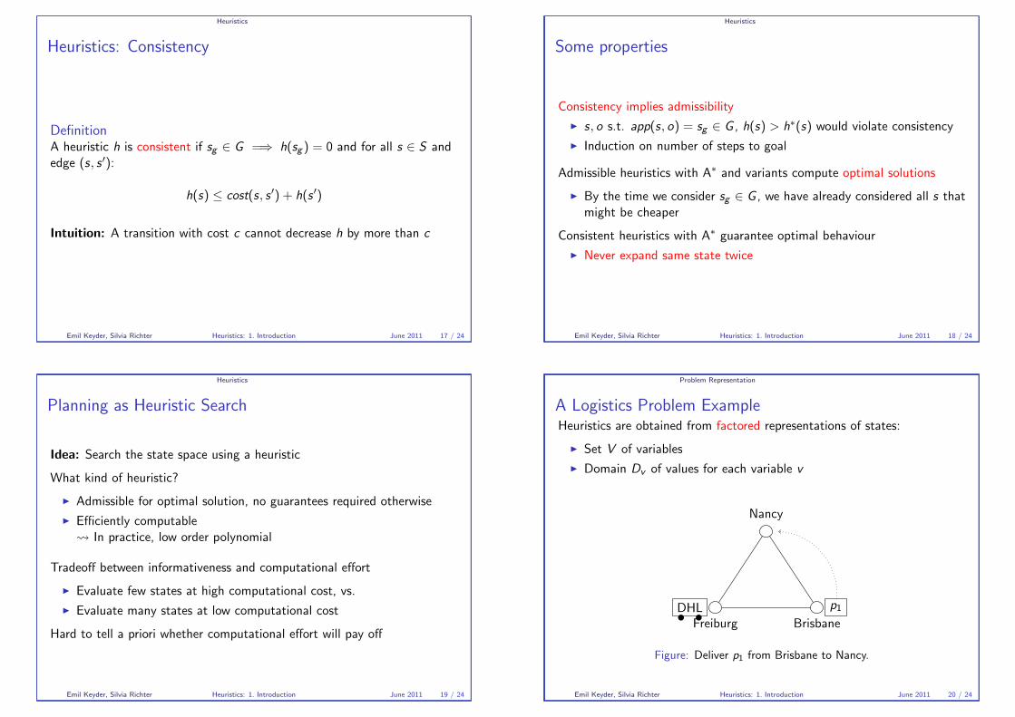
A heuristic h is consistent if sg ∈ G =⇒ h(sg ) = 0 and for all s ∈ S andedge (s, s �):
h(s) ≤ cost(s, s �) + h(s �)
Intuition: A transition with cost c cannot decrease h by more than c
Emil Keyder, Silvia Richter Heuristics: 1. Introduction June 2011 17 / 24
Heuristics
Some properties
Consistency implies admissibility
� s, o s.t. app(s, o) = sg ∈ G , h(s) > h∗(s) would violate consistency
� Induction on number of steps to goal
Admissible heuristics with A∗ and variants compute optimal solutions
� By the time we consider sg ∈ G , we have already considered all s thatmight be cheaper
Consistent heuristics with A∗ guarantee optimal behaviour
� Never expand same state twice
Emil Keyder, Silvia Richter Heuristics: 1. Introduction June 2011 18 / 24
Heuristics
Planning as Heuristic Search
Idea: Search the state space using a heuristic
What kind of heuristic?
� Admissible for optimal solution, no guarantees required otherwise
� Efficiently computable� In practice, low order polynomial
Tradeoff between informativeness and computational effort
� Evaluate few states at high computational cost, vs.
� Evaluate many states at low computational cost
Hard to tell a priori whether computational effort will pay off
Emil Keyder, Silvia Richter Heuristics: 1. Introduction June 2011 19 / 24
Problem Representation
A Logistics Problem Example
Heuristics are obtained from factored representations of states:
� Set V of variables
� Domain Dv of values for each variable v
Freiburg Brisbane
Nancy
DHL p1
Figure: Deliver p1 from Brisbane to Nancy.
Emil Keyder, Silvia Richter Heuristics: 1. Introduction June 2011 20 / 24
Problem Representation
STRIPS
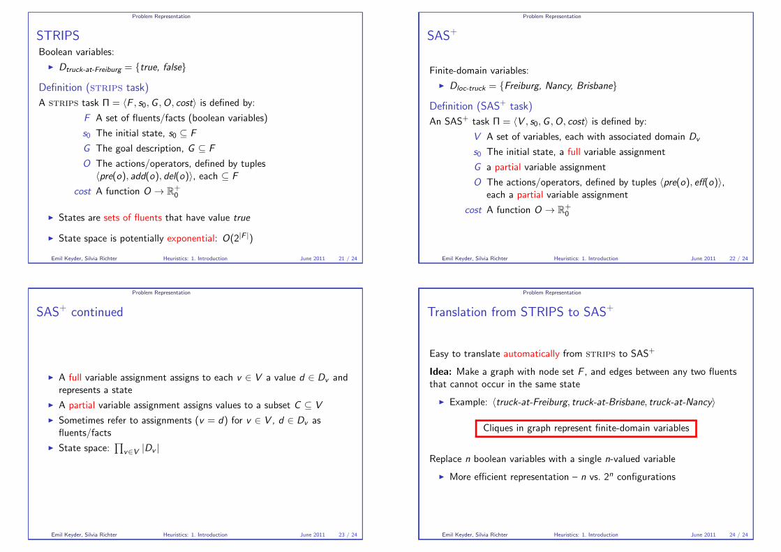
Boolean variables:
� Dtruck-at-Freiburg = {true, false}
Definition (strips task)
A strips task Π = �F , s0,G ,O, cost� is defined by:
F A set of fluents/facts (boolean variables)
s0 The initial state, s0 ⊆ F
G The goal description, G ⊆ F
O The actions/operators, defined by tuples�pre(o), add(o), del(o)�, each ⊆ F
cost A function O → R+
0
� States are sets of fluents that have value true
� State space is potentially exponential: O(2|F |)
Emil Keyder, Silvia Richter Heuristics: 1. Introduction June 2011 21 / 24
Problem Representation
SAS+
Finite-domain variables:
� Dloc-truck = {Freiburg, Nancy, Brisbane}
Definition (SAS+task)
An SAS+ task Π = �V , s0,G ,O, cost� is defined by:
V A set of variables, each with associated domain Dv
s0 The initial state, a full variable assignment
G a partial variable assignment
O The actions/operators, defined by tuples �pre(o), eff(o)�,each a partial variable assignment
cost A function O → R+
0
Emil Keyder, Silvia Richter Heuristics: 1. Introduction June 2011 22 / 24
Problem Representation
SAS+continued
� A full variable assignment assigns to each v ∈ V a value d ∈ Dv andrepresents a state
� A partial variable assignment assigns values to a subset C ⊆ V
� Sometimes refer to assignments (v = d) for v ∈ V , d ∈ Dv asfluents/facts
� State space:�
v∈V |Dv |
Emil Keyder, Silvia Richter Heuristics: 1. Introduction June 2011 23 / 24
Problem Representation
Translation from STRIPS to SAS+
Easy to translate automatically from strips to SAS+
Idea: Make a graph with node set F , and edges between any two fluentsthat cannot occur in the same state
� Example: �truck-at-Freiburg, truck-at-Brisbane, truck-at-Nancy�
Cliques in graph represent finite-domain variables
Replace n boolean variables with a single n-valued variable
� More efficient representation – n vs. 2n configurations
Emil Keyder, Silvia Richter Heuristics: 1. Introduction June 2011 24 / 24
Heuristics for Domain-Independent Planning
2. The Delete Relaxation
Emil Keyder Silvia Richter
ICAPS 2011 Summer School on Automated Planning and Scheduling
June 2011
Emil Keyder, Silvia Richter Heuristics: 2. Delete Relaxation June 2011 1 / 49
The Delete RelaxationDefinitionSources of Difficulty in Π+
hmax & hadd
The Max Heuristic hmax
The Additive Heuristic hadd
Computation
Relaxed Plan HeuristicsThe FF Heuristic hFF
Relaxed Plans with Cost-Sensitive Best SupportersThe Set-Additive Heuristic haddset
Beyond the Independence Assumption
Conclusions
Emil Keyder, Silvia Richter Heuristics: 2. Delete Relaxation June 2011 2 / 49
Π+
Definition
Relaxations
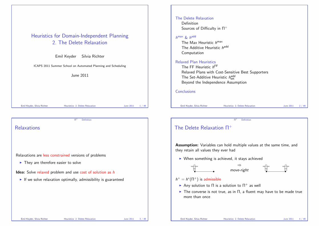
Relaxations are less constrained versions of problems
� They are therefore easier to solve
Idea: Solve relaxed problem and use cost of solution as h
� If we solve relaxation optimally, admissibility is guaranteed
Emil Keyder, Silvia Richter Heuristics: 2. Delete Relaxation June 2011 3 / 49
Π+
Definition
The Delete Relaxation Π+
Assumption: Variables can hold multiple values at the same time, andthey retain all values they ever had
� When something is achieved, it stays achieved
⇒move-right
h+ = h∗(Π+) is admissible
� Any solution to Π is a solution to Π+ as well
� The converse is not true, as in Π, a fluent may have to be made truemore than once
Emil Keyder, Silvia Richter Heuristics: 2. Delete Relaxation June 2011 4 / 49
Π+
Definition
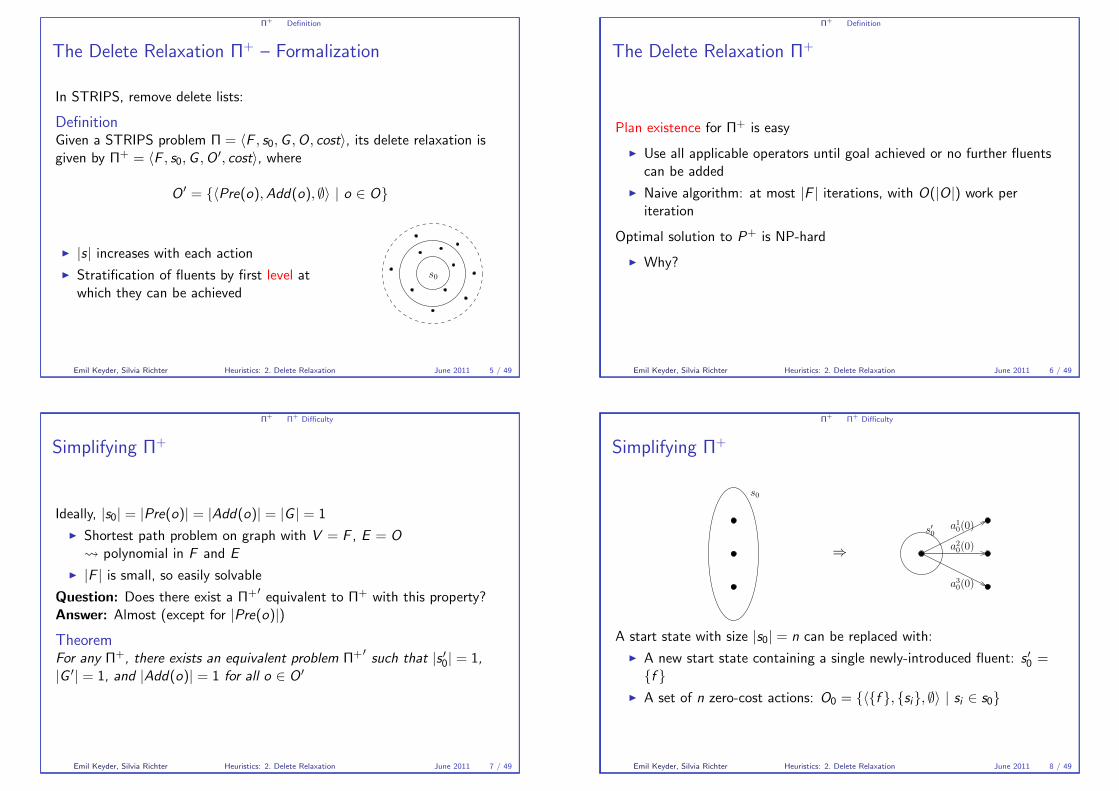
The Delete Relaxation Π+– Formalization
In STRIPS, remove delete lists:
Definition
Given a STRIPS problem Π = �F , s0,G ,O, cost�, its delete relaxation isgiven by Π+ = �F , s0,G ,O �, cost�, where
O� = {�Pre(o),Add(o), ∅� | o ∈ O}
� |s| increases with each action
� Stratification of fluents by first level atwhich they can be achieved
s0
Emil Keyder, Silvia Richter Heuristics: 2. Delete Relaxation June 2011 5 / 49
Π+
Definition
The Delete Relaxation Π+
Plan existence for Π+ is easy
� Use all applicable operators until goal achieved or no further fluentscan be added
� Naive algorithm: at most |F | iterations, with O(|O|) work periteration
Optimal solution to P+ is NP-hard
� Why?
Emil Keyder, Silvia Richter Heuristics: 2. Delete Relaxation June 2011 6 / 49
Π+
Π+
Difficulty
Simplifying Π+
Ideally, |s0| = |Pre(o)| = |Add(o)| = |G | = 1
� Shortest path problem on graph with V = F , E = O
� polynomial in F and E
� |F | is small, so easily solvable
Question: Does there exist a Π+� equivalent to Π+ with this property?Answer: Almost (except for |Pre(o)|)
Theorem
For any Π+, there exists an equivalent problem Π+�such that |s �
0| = 1,
|G �| = 1, and |Add(o)| = 1 for all o ∈ O �
Emil Keyder, Silvia Richter Heuristics: 2. Delete Relaxation June 2011 7 / 49
Π+
Π+
Difficulty
Simplifying Π+
s0
⇒
a30(0)
s�0a10(0)
a20(0)
A start state with size |s0| = n can be replaced with:
� A new start state containing a single newly-introduced fluent: s �0=
{f }� A set of n zero-cost actions: O0 = {�{f }, {si}, ∅� | si ∈ s0}
Emil Keyder, Silvia Richter Heuristics: 2. Delete Relaxation June 2011 8 / 49
Π+
Π+
Difficulty
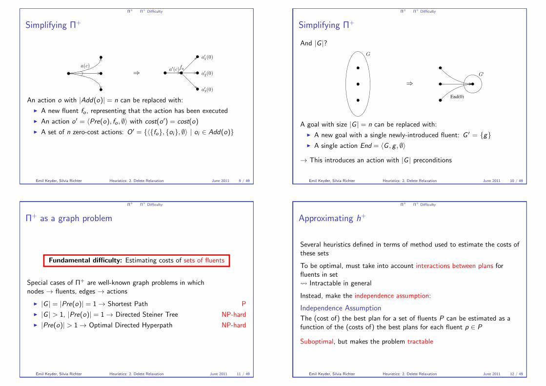
Simplifying Π+
a(c)
⇒
a�3(0)
faa�(c)
a�1(0)
a�2(0)
An action o with |Add(o)| = n can be replaced with:
� A new fluent fo , representing that the action has been executed
� An action o � = �Pre(o), fo , ∅� with cost(o �) = cost(o)
� A set of n zero-cost actions: O � = {�{fo}, {oi}, ∅� | oi ∈ Add(o)}
Emil Keyder, Silvia Richter Heuristics: 2. Delete Relaxation June 2011 9 / 49
Π+
Π+
Difficulty
Simplifying Π+
And |G |?G
⇒
End(0)
G�
A goal with size |G | = n can be replaced with:
� A new goal with a single newly-introduced fluent: G � = {g}� A single action End = �G , g , ∅�
→ This introduces an action with |G | preconditions
Emil Keyder, Silvia Richter Heuristics: 2. Delete Relaxation June 2011 10 / 49
Π+
Π+
Difficulty
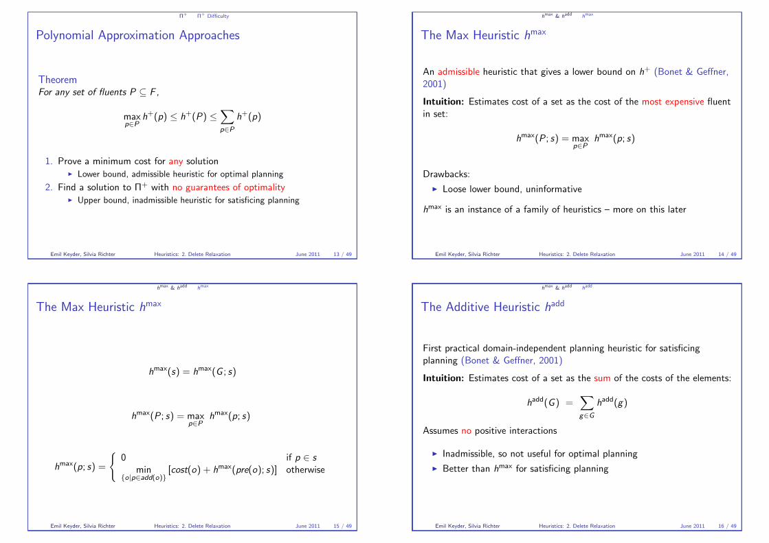
Π+as a graph problem
Fundamental difficulty: Estimating costs of sets of fluents
Special cases of Π+ are well-known graph problems in whichnodes → fluents, edges → actions
� |G | = |Pre(o)| = 1 → Shortest Path P
� |G | > 1, |Pre(o)| = 1 → Directed Steiner Tree NP-hard
� |Pre(o)| > 1 → Optimal Directed Hyperpath NP-hard
Emil Keyder, Silvia Richter Heuristics: 2. Delete Relaxation June 2011 11 / 49
Π+
Π+
Difficulty
Approximating h+
Several heuristics defined in terms of method used to estimate the costs ofthese sets
To be optimal, must take into account interactions between plans forfluents in set� Intractable in general
Instead, make the independence assumption:
Independence Assumption
The (cost of) the best plan for a set of fluents P can be estimated as afunction of the (costs of) the best plans for each fluent p ∈ P
Suboptimal, but makes the problem tractable
Emil Keyder, Silvia Richter Heuristics: 2. Delete Relaxation June 2011 12 / 49
Π+
Π+
Difficulty
Polynomial Approximation Approaches
Theorem
For any set of fluents P ⊆ F ,
maxp∈P
h+(p) ≤ h
+(P) ≤�
p∈Ph+(p)
1. Prove a minimum cost for any solution� Lower bound, admissible heuristic for optimal planning
2. Find a solution to Π+ with no guarantees of optimality� Upper bound, inadmissible heuristic for satisficing planning
Emil Keyder, Silvia Richter Heuristics: 2. Delete Relaxation June 2011 13 / 49
hmax
& hadd
hmax
The Max Heuristic hmax
An admissible heuristic that gives a lower bound on h+ (Bonet & Geffner,2001)
Intuition: Estimates cost of a set as the cost of the most expensive fluentin set:
hmax(P ; s) = max
p∈Phmax(p; s)
Drawbacks:
� Loose lower bound, uninformative
hmax is an instance of a family of heuristics – more on this later
Emil Keyder, Silvia Richter Heuristics: 2. Delete Relaxation June 2011 14 / 49
hmax
& hadd
hmax
The Max Heuristic hmax
hmax(s) = h
max(G ; s)
hmax(P ; s) = max
p∈Phmax(p; s)
hmax(p; s) =
�0 if p ∈ s
min{o|p∈add(o)}
[cost(o) + hmax(pre(o); s)] otherwise
Emil Keyder, Silvia Richter Heuristics: 2. Delete Relaxation June 2011 15 / 49
hmax
& hadd
hadd
The Additive Heuristic hadd
First practical domain-independent planning heuristic for satisficingplanning (Bonet & Geffner, 2001)
Intuition: Estimates cost of a set as the sum of the costs of the elements:
hadd(G ) =
�
g∈Ghadd(g)
Assumes no positive interactions
� Inadmissible, so not useful for optimal planning
� Better than hmax for satisficing planning
Emil Keyder, Silvia Richter Heuristics: 2. Delete Relaxation June 2011 16 / 49
hmax
& hadd
hadd
The Additive Heuristic hadd
hadd(s) = h
add(G ; s)
hadd(P ; s) =
�
p∈Phadd(p; s)
hadd(p; s) =
0 if p ∈ s
min{o|p∈add(o)}
�cost(o) + h
add(pre(o); s)�
otherwise
Emil Keyder, Silvia Richter Heuristics: 2. Delete Relaxation June 2011 17 / 49
hmax
& hadd
Computation
Computation
Equations give properties of estimates, not how to calculate them
Basic idea: value iteration
� Start with rough estimates (e.g. 0,∞), do updates
Methods differ principally in choice of update ordering:
1. Label-correcting methods
� Arbitrary action choice� Multiple updates per fluent
2. Dijkstra method
� Updates placed in priority queue� Single update per fluent
Emil Keyder, Silvia Richter Heuristics: 2. Delete Relaxation June 2011 18 / 49
hmax
& hadd
Computation
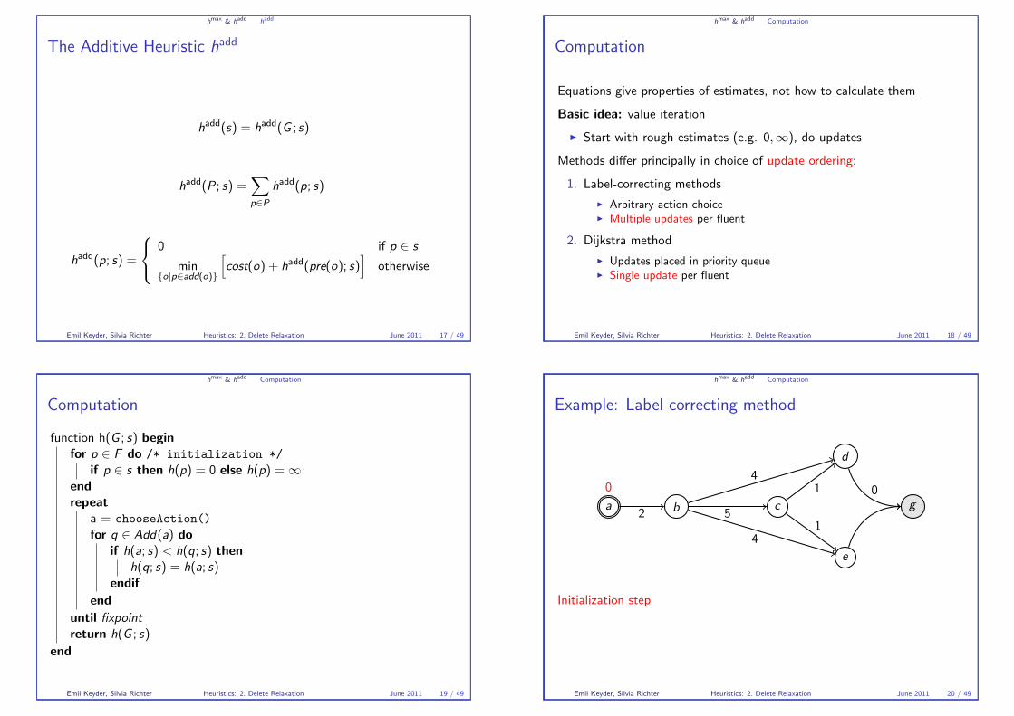
Computation
function h(G ; s) beginfor p ∈ F do /* initialization */
if p ∈ s then h(p) = 0 else h(p) = ∞endrepeat
a = chooseAction()
for q ∈ Add(a) doif h(a; s) < h(q; s) then
h(q; s) = h(a; s)endif
enduntil fixpointreturn h(G ; s)
end
Emil Keyder, Silvia Richter Heuristics: 2. Delete Relaxation June 2011 19 / 49
hmax
& hadd
Computation
Example: Label correcting method
a
0
b2c
5
d
41
e
41
g
0
Initialization step
Emil Keyder, Silvia Richter Heuristics: 2. Delete Relaxation June 2011 20 / 49
hmax
& hadd
Computation
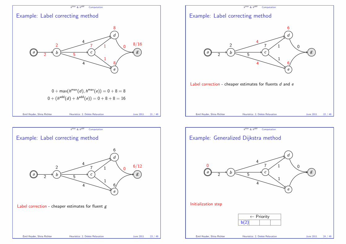
Example: Label correcting method
a b
2
2c
7
5
d
8
41
e
841
g
8/160
0 + max(hmax(d), hmax(e)) = 0 + 8 = 8
0 + (hadd(d) + hadd(e)) = 0 + 8 + 8 = 16
Emil Keyder, Silvia Richter Heuristics: 2. Delete Relaxation June 2011 21 / 49
hmax
& hadd
Computation
Example: Label correcting method
a b
2
2c
7
5
d
6
41
e
641
g
0
Label correction - cheaper estimates for fluents d and e
Emil Keyder, Silvia Richter Heuristics: 2. Delete Relaxation June 2011 22 / 49
hmax
& hadd
Computation
Example: Label correcting method
a b
2
2c
7
5
d
6
41
e
641
g
6/120
Label correction - cheaper estimates for fluent g
Emil Keyder, Silvia Richter Heuristics: 2. Delete Relaxation June 2011 23 / 49
hmax
& hadd
Computation
Example: Generalized Dijkstra method
a
0
b2c
7
5
d
41
e
41
g
0
Initialization step
← Priorityb(2)
Emil Keyder, Silvia Richter Heuristics: 2. Delete Relaxation June 2011 24 / 49

hmax
& hadd
Computation
Example: Generalized Dijkstra method
a
0
b
2
2c
7
5
d
41
e
41
g
0
← Priorityd(6) e(6) c(7)
Emil Keyder, Silvia Richter Heuristics: 2. Delete Relaxation June 2011 25 / 49
hmax
& hadd
Computation
Example: Generalized Dijkstra method
a
0
b
2
2c
7
5
d
6
41
e
641
g
0
g has priority 6 when computing hmax
� would have priority 12 when computing hadd
← Priorityg(6) c(7)
Emil Keyder, Silvia Richter Heuristics: 2. Delete Relaxation June 2011 26 / 49
hmax
& hadd
Computation
Example: Generalized Dijkstra method
a
0
b
2
2c
7
5
d
6
41
e
641
g
60
Can stop when all goals are reached – Generalized Dijkstra guarantees singleupdate, so goal costs won’t decrease
← Priorityc(7)
Emil Keyder, Silvia Richter Heuristics: 2. Delete Relaxation June 2011 27 / 49
hmax
& hadd
Computation
Comments
Generalized Dijkstra performs single update per fluent
� Slower due to overhead from priority queue
In practice, Generalized Bellman-Ford often used
� However, GD + incremental computation shown to give speedup(Liu, Koenig, and Furcy, 2002)
Emil Keyder, Silvia Richter Heuristics: 2. Delete Relaxation June 2011 28 / 49
hmax
& hadd
Computation
Problems with hadd
a b2c
5
d
41
e
41
g
0
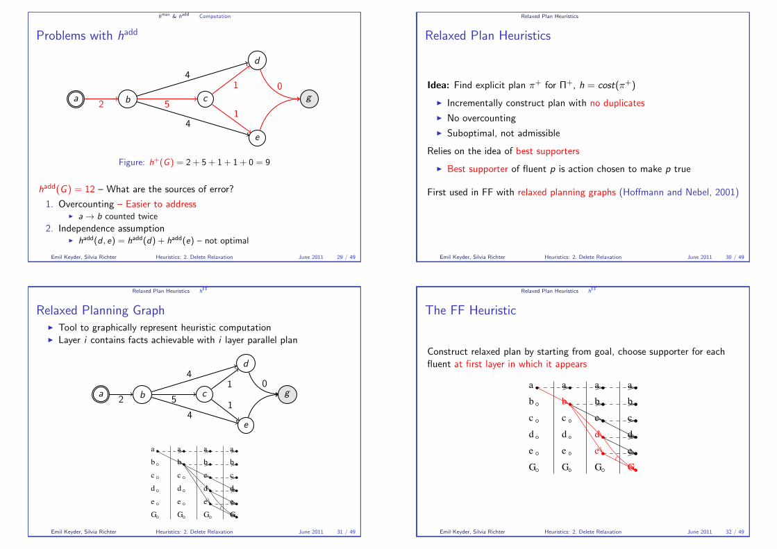
Figure: h+(G ) = 2 + 5 + 1 + 1 + 0 = 9
hadd(G ) = 12 – What are the sources of error?
1. Overcounting – Easier to address� a → b counted twice
2. Independence assumption� hadd(d , e) = hadd(d) + hadd(e) – not optimal
Emil Keyder, Silvia Richter Heuristics: 2. Delete Relaxation June 2011 29 / 49
Relaxed Plan Heuristics
Relaxed Plan Heuristics
Idea: Find explicit plan π+ for Π+, h = cost(π+)
� Incrementally construct plan with no duplicates
� No overcounting
� Suboptimal, not admissible
Relies on the idea of best supporters
� Best supporter of fluent p is action chosen to make p true
First used in FF with relaxed planning graphs (Hoffmann and Nebel, 2001)
Emil Keyder, Silvia Richter Heuristics: 2. Delete Relaxation June 2011 30 / 49
Relaxed Plan Heuristics hFF
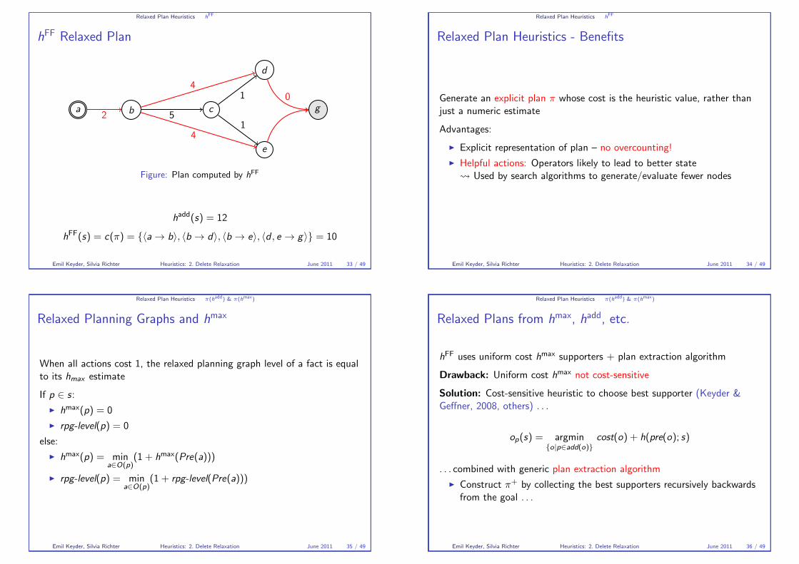
Relaxed Planning Graph
� Tool to graphically represent heuristic computation� Layer i contains facts achievable with i layer parallel plan
a b2c
5
d
41
e
41
g0
c
a
b
G
e
d
c
a
b
G
e
d
c
a
b
e
d
c
G
a
b
G
e
d
Emil Keyder, Silvia Richter Heuristics: 2. Delete Relaxation June 2011 31 / 49
Relaxed Plan Heuristics hFF
The FF Heuristic
Construct relaxed plan by starting from goal, choose supporter for eachfluent at first layer in which it appears
d
a
b
G
e
d
c
a
b
G
e
c
a
b
e
d
c
G
a
b
G
e
d
c
Emil Keyder, Silvia Richter Heuristics: 2. Delete Relaxation June 2011 32 / 49
Relaxed Plan Heuristics hFF
hFF Relaxed Plan
a b2c
5
d
41
e
41
g
0
Figure: Plan computed by hFF
hadd(s) = 12
hFF(s) = c(π) = {�a → b�, �b → d�, �b → e�, �d , e → g�} = 10
Emil Keyder, Silvia Richter Heuristics: 2. Delete Relaxation June 2011 33 / 49
Relaxed Plan Heuristics hFF
Relaxed Plan Heuristics - Benefits
Generate an explicit plan π whose cost is the heuristic value, rather thanjust a numeric estimate
Advantages:
� Explicit representation of plan – no overcounting!
� Helpful actions: Operators likely to lead to better state� Used by search algorithms to generate/evaluate fewer nodes
Emil Keyder, Silvia Richter Heuristics: 2. Delete Relaxation June 2011 34 / 49
Relaxed Plan Heuristics π(hadd
) & π(hmax
)
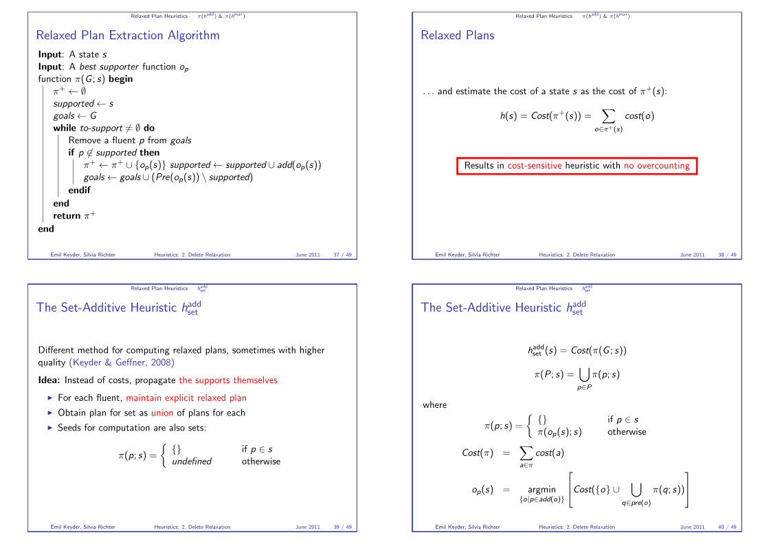
Relaxed Planning Graphs and hmax
When all actions cost 1, the relaxed planning graph level of a fact is equalto its hmax estimate
If p ∈ s:
� hmax(p) = 0
� rpg-level(p) = 0
else:
� hmax(p) = mina∈O(p)
(1 + hmax(Pre(a)))
� rpg-level(p) = mina∈O(p)
(1 + rpg-level(Pre(a)))
Emil Keyder, Silvia Richter Heuristics: 2. Delete Relaxation June 2011 35 / 49
Relaxed Plan Heuristics π(hadd
) & π(hmax
)
Relaxed Plans from hmax, hadd, etc.
hFF uses uniform cost hmax supporters + plan extraction algorithm
Drawback: Uniform cost hmax not cost-sensitive
Solution: Cost-sensitive heuristic to choose best supporter (Keyder &Geffner, 2008, others) . . .
op(s) = argmin{o|p∈add(o)}
cost(o) + h(pre(o); s)
. . . combined with generic plan extraction algorithm
� Construct π+ by collecting the best supporters recursively backwardsfrom the goal . . .
Emil Keyder, Silvia Richter Heuristics: 2. Delete Relaxation June 2011 36 / 49
Relaxed Plan Heuristics π(hadd
) & π(hmax
)
Relaxed Plan Extraction Algorithm
Input: A state s
Input: A best supporter function op
function π(G ; s) beginπ+ ← ∅supported ← s
goals ← G
while to-support �= ∅ doRemove a fluent p from goals
if p �∈ supported thenπ+ ← π+ ∪ {op(s)} supported ← supported ∪ add(op(s))goals ← goals ∪ (Pre(op(s)) \ supported)
endifendreturn π+
end
Emil Keyder, Silvia Richter Heuristics: 2. Delete Relaxation June 2011 37 / 49
Relaxed Plan Heuristics π(hadd
) & π(hmax
)
Relaxed Plans
. . . and estimate the cost of a state s as the cost of π+(s):
h(s) = Cost(π+(s)) =�
o∈π+(s)
cost(o)
Results in cost-sensitive heuristic with no overcounting
Emil Keyder, Silvia Richter Heuristics: 2. Delete Relaxation June 2011 38 / 49
Relaxed Plan Heuristics hadd
set
The Set-Additive Heuristic haddset
Different method for computing relaxed plans, sometimes with higherquality (Keyder & Geffner, 2008)
Idea: Instead of costs, propagate the supports themselves
� For each fluent, maintain explicit relaxed plan
� Obtain plan for set as union of plans for each
� Seeds for computation are also sets:
π(p; s) =
�{} if p ∈ s
undefined otherwise
Emil Keyder, Silvia Richter Heuristics: 2. Delete Relaxation June 2011 39 / 49
Relaxed Plan Heuristics hadd
set
The Set-Additive Heuristic haddset
hadd
set (s) = Cost(π(G ; s))
π(P ; s) =�
p∈Pπ(p; s)
where
π(p; s) =
�{} if p ∈ s
π(op(s); s) otherwise
Cost(π) =�
a∈πcost(a)
op(s) = argmin{o|p∈add(o)}
Cost({o} ∪�
q∈pre(o)
π(q; s))
Emil Keyder, Silvia Richter Heuristics: 2. Delete Relaxation June 2011 40 / 49
Relaxed Plan Heuristics hadd
set
The Set-Additive Heuristic haddset
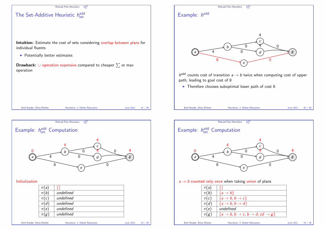
Intuition: Estimate the cost of sets considering overlap between plans forindividual fluents
� Potentially better estimates
Drawback: ∪ operation expensive compared to cheaper�
or maxoperation
Emil Keyder, Silvia Richter Heuristics: 2. Delete Relaxation June 2011 41 / 49
Relaxed Plan Heuristics hadd
set
Example: hadd
a
b
4
c
4
0
d
4
0
e6
g
0
0
hadd counts cost of transition a → b twice when computing cost of upperpath, leading to goal cost of 8
� Therefore chooses suboptimal lower path of cost 6
Emil Keyder, Silvia Richter Heuristics: 2. Delete Relaxation June 2011 42 / 49
Relaxed Plan Heuristics hadd
set
Example: haddset Computation
a
0 b
4
4
c
4
0
d
4
0
e6
g
4
0
0
Initialization
π(a) {}π(b) undefined
π(c) undefined
π(d) undefined
π(e) undefined
π(g) undefined
Emil Keyder, Silvia Richter Heuristics: 2. Delete Relaxation June 2011 43 / 49
Relaxed Plan Heuristics hadd
set
Example: haddset Computation
a
0 b
4
4
c
4
0
d
4
0
e6
g
4
0
0
a → b counted only once when taking union of plans
π(a) {}π(b) {a → b}π(c) {a → b, b → c}π(d) {a → b, b → d}π(e) undefined
π(g) {a → b, b → c , b → d , cd → g}
Emil Keyder, Silvia Richter Heuristics: 2. Delete Relaxation June 2011 44 / 49
Relaxed Plan Heuristics hadd
set
a
b
4
c
0
d0
e6
g
0
0
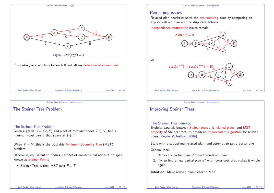
Figure: cost(πaddset ) = 4
Computing relaxed plans for each fluent allows detection of shared cost
Emil Keyder, Silvia Richter Heuristics: 2. Delete Relaxation June 2011 45 / 49
Relaxed Plan Heuristics Independence
Remaining issues
Relaxed-plan heuristics solve the overcounting issue by computing anexplicit relaxed plan with no duplicate actions
Independence assumption issues remain
cost(π∗) = 9
a b2c
5
d4
1
e4
1g
0
vs.
cost(πadd) = cost(πmax) = 10
a b2c
5
d4
1
e4
1g
0
Emil Keyder, Silvia Richter Heuristics: 2. Delete Relaxation June 2011 46 / 49
Relaxed Plan Heuristics Independence
The Steiner Tree Problem
The Steiner Tree Problem
Given a graph G = �V ,E � and a set of terminal nodes T ⊆ V , find aminimum-cost tree S that spans all t ∈ T
When T = V , this is the tractable Minimum Spanning Tree (MST)problem
Otherwise, equivalent to finding best set of non-terminal nodes P to span,known as Steiner Points
� Steiner Tree is then MST over P ∪ T
Emil Keyder, Silvia Richter Heuristics: 2. Delete Relaxation June 2011 47 / 49
Relaxed Plan Heuristics Independence
Improving Steiner Trees
The Steiner Tree heuristic
Exploits parallels between Steiner trees and relaxed plans, and MSTproperty of Steiner trees, to obtain an improvement algorithm for relaxedplans (Keyder & Geffner, 2009)
Start with a suboptimal relaxed plan, and attempt to get a better one
General idea:
1. Remove a partial plan π� from the relaxed plan
2. Try to find a new partial plan π�� with lower cost that makes it wholeagain
Intuition: Make relaxed plan closer to MST
Emil Keyder, Silvia Richter Heuristics: 2. Delete Relaxation June 2011 48 / 49
Conclusions
Conclusions
� The optimal delete relaxation heuristic h+ is admissible andinformative, but calculating it is NP-hard
� Sub-optimal solutions have proven to be effective heuristics forsatisficing planning
� hadd suffers from two problems:1. Overcounting of actions when combining estimates
2. The independence assumption
� Overcounting problem can be solved with relaxed-plan heuristics� Cost-sensitive best supporters
� Steiner Tree heuristic is an attempt at improving estimates obtainedwith the independence assumption
Emil Keyder, Silvia Richter Heuristics: 2. Delete Relaxation June 2011 49 / 49
Heuristics for Domain-Independent Planning
3. Critical Path Heuristics
Emil Keyder Silvia Richter
ICAPS 2011 Summer School on Automated Planning and Scheduling
June 2011
Emil Keyder, Silvia Richter Heuristics: 3. Critical Path June 2011 1 / 13
hmax= h1
hm Heuristics
The Πm Compilation
Summary
Emil Keyder, Silvia Richter Heuristics: 3. Critical Path June 2011 2 / 13
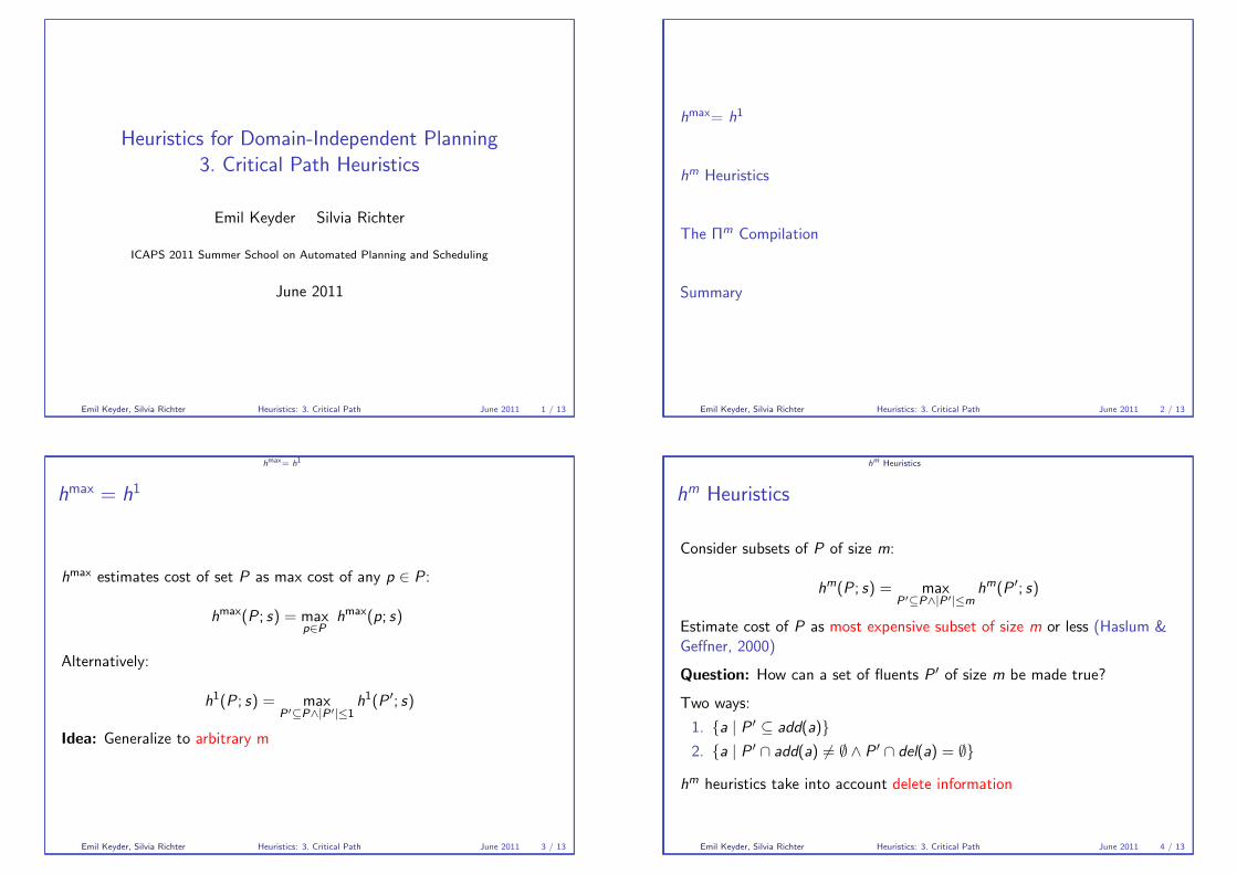
hmax= h1
hmax= h1
hmax estimates cost of set P as max cost of any p ∈ P :
hmax(P ; s) = max
p∈Phmax(p; s)
Alternatively:
h1(P ; s) = max
P�⊆P∧|P�|≤1
h1(P �; s)
Idea: Generalize to arbitrary m
Emil Keyder, Silvia Richter Heuristics: 3. Critical Path June 2011 3 / 13
hm Heuristics
hm Heuristics
Consider subsets of P of size m:
hm(P ; s) = max
P�⊆P∧|P�|≤mhm(P �; s)
Estimate cost of P as most expensive subset of size m or less (Haslum &Geffner, 2000)
Question: How can a set of fluents P � of size m be made true?
Two ways:
1. {a | P � ⊆ add(a)}2. {a | P � ∩ add(a) �= ∅ ∧ P � ∩ del(a) = ∅}
hm heuristics take into account delete information
Emil Keyder, Silvia Richter Heuristics: 3. Critical Path June 2011 4 / 13
hm Heuristics
Example
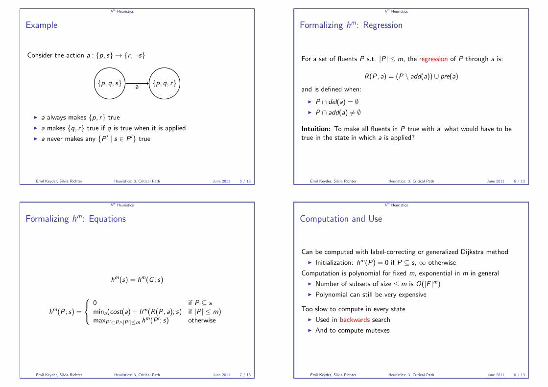
Consider the action a : {p, s} → {r ,¬s}
{p, q, s} {p, q, r}a
� a always makes {p, r} true
� a makes {q, r} true if q is true when it is applied
� a never makes any {P � | s ∈ P �} true
Emil Keyder, Silvia Richter Heuristics: 3. Critical Path June 2011 5 / 13
hm Heuristics
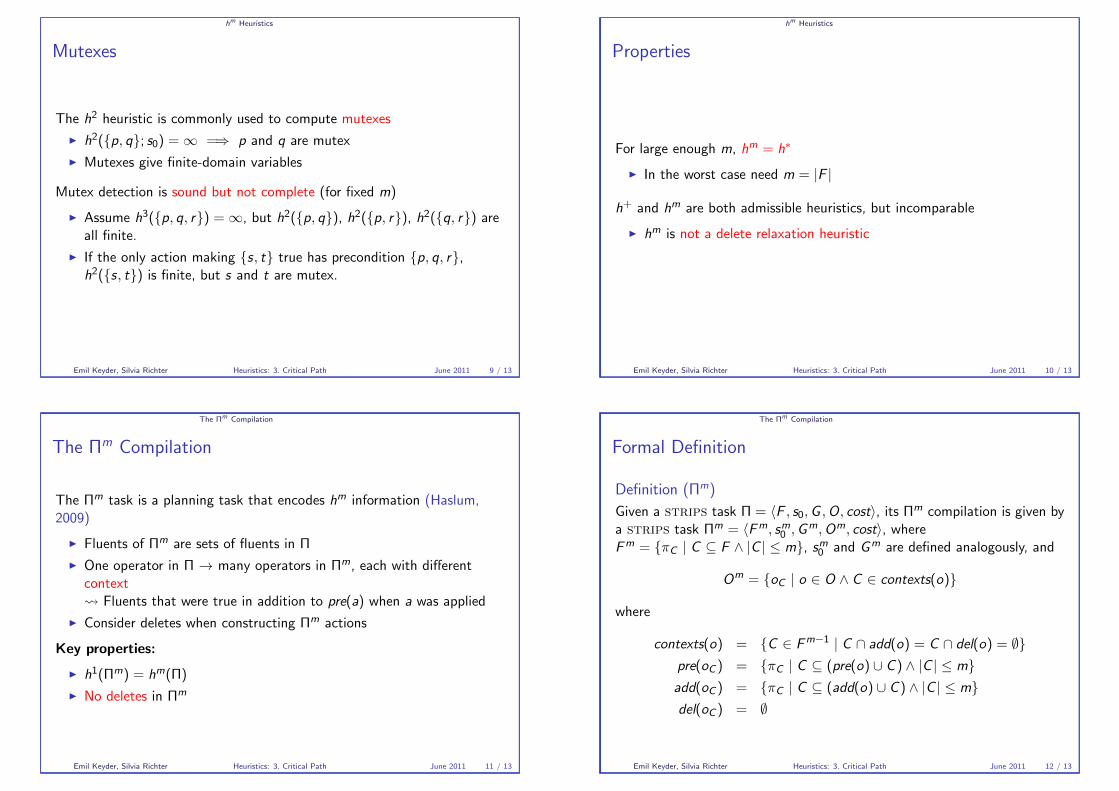
Formalizing hm: Regression
For a set of fluents P s.t. |P | ≤ m, the regression of P through a is:
R(P , a) = (P \ add(a)) ∪ pre(a)
and is defined when:
� P ∩ del(a) = ∅� P ∩ add(a) �= ∅
Intuition: To make all fluents in P true with a, what would have to betrue in the state in which a is applied?
Emil Keyder, Silvia Richter Heuristics: 3. Critical Path June 2011 6 / 13
hm Heuristics
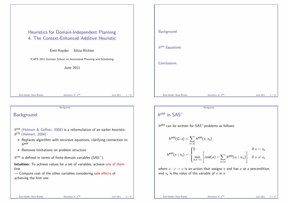
Formalizing hm: Equations
hm(s) = h
m(G ; s)
hm(P ; s) =
0 if P ⊆ s
mina(cost(a) + hm(R(P , a); s) if |P | ≤ m)maxP�⊂P∧|P�|≤m hm(P �; s) otherwise
Emil Keyder, Silvia Richter Heuristics: 3. Critical Path June 2011 7 / 13
hm Heuristics
Computation and Use
Can be computed with label-correcting or generalized Dijkstra method
� Initialization: hm(P) = 0 if P ⊆ s, ∞ otherwise
Computation is polynomial for fixed m, exponential in m in general
� Number of subsets of size ≤ m is O(|F |m)� Polynomial can still be very expensive
Too slow to compute in every state
� Used in backwards search
� And to compute mutexes
Emil Keyder, Silvia Richter Heuristics: 3. Critical Path June 2011 8 / 13
hm Heuristics
Mutexes
The h2 heuristic is commonly used to compute mutexes
� h2({p, q}; s0) = ∞ =⇒ p and q are mutex
� Mutexes give finite-domain variables
Mutex detection is sound but not complete (for fixed m)
� Assume h3({p, q, r}) = ∞, but h2({p, q}), h2({p, r}), h2({q, r}) areall finite.
� If the only action making {s, t} true has precondition {p, q, r},h2({s, t}) is finite, but s and t are mutex.
Emil Keyder, Silvia Richter Heuristics: 3. Critical Path June 2011 9 / 13
hm Heuristics
Properties
For large enough m, hm = h∗
� In the worst case need m = |F |
h+ and hm are both admissible heuristics, but incomparable
� hm is not a delete relaxation heuristic
Emil Keyder, Silvia Richter Heuristics: 3. Critical Path June 2011 10 / 13
The Πm
Compilation
The ΠmCompilation
The Πm task is a planning task that encodes hm information (Haslum,2009)
� Fluents of Πm are sets of fluents in Π
� One operator in Π → many operators in Πm, each with differentcontext� Fluents that were true in addition to pre(a) when a was applied
� Consider deletes when constructing Πm actions
Key properties:
� h1(Πm) = hm(Π)
� No deletes in Πm
Emil Keyder, Silvia Richter Heuristics: 3. Critical Path June 2011 11 / 13
The Πm
Compilation
Formal Definition
Definition (Πm)
Given a strips task Π = �F , s0,G ,O, cost�, its Πm compilation is given bya strips task Πm = �Fm, sm
0,Gm,Om, cost�, where
Fm = {πC | C ⊆ F ∧ |C | ≤ m}, sm0
and Gm are defined analogously, and
Om = {oC | o ∈ O ∧ C ∈ contexts(o)}
where
contexts(o) = {C ∈ Fm−1 | C ∩ add(o) = C ∩ del(o) = ∅}
pre(oC ) = {πC | C ⊆ (pre(o) ∪ C ) ∧ |C | ≤ m}add(oC ) = {πC | C ⊆ (add(o) ∪ C ) ∧ |C | ≤ m}del(oC ) = ∅
Emil Keyder, Silvia Richter Heuristics: 3. Critical Path June 2011 12 / 13

Summary
Conclusions
� hm heuristics are admissible estimates obtained by considering criticalpaths
� hm heuristics take deletes into account, and are incomparable to h+
� Their computation is polynomial for fixed m, but exponential in m ingeneral
� As m → |F |, hm(s) → h∗(s)
Emil Keyder, Silvia Richter Heuristics: 3. Critical Path June 2011 13 / 13
Heuristics for Domain-Independent Planning4. The Context-Enhanced Additive Heuristic
Emil Keyder Silvia Richter
ICAPS 2011 Summer School on Automated Planning and Scheduling
June 2011
Emil Keyder, Silvia Richter Heuristics: X. hcea June 2011 1 / 17
Background
hcea Equations
Conclusions
Emil Keyder, Silvia Richter Heuristics: X. hcea June 2011 2 / 17
Background
Background
hcea (Helmert & Geffner, 2008) is a reformulation of an earlier heuristic,hCG (Helmert, 2004)
� Replaces algorithm with recursive equations, clarifying connection tohadd
� Removes limitations on problem structure
hcea is defined in terms of finite-domain variables (SAS+)
Intuition: To achieve values for a set of variables, achieve one of themfirst� Compute cost of the other variables considering side effects ofachieving the first one
Emil Keyder, Silvia Richter Heuristics: X. hcea June 2011 3 / 17
Background
hadd in SAS+
hadd can be written for SAS+problems as follows:
hadd(G ; s) =
�
x∈Ghadd(x ; xs)
hadd(x | xs) =
0 if x = xs
mino:z→x
�cost(o) +
�
xi∈zhadd(xi | xi s)
�if x �= xs
where o : z → x is an action that assigns x and has z as a precondition,and xs is the value of the variable of x in s.
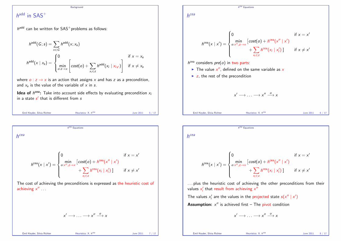
Idea of hcea: Take into account side effects by evaluating precondition xi
in a state s � that is different from s
Emil Keyder, Silvia Richter Heuristics: X. hcea June 2011 4 / 17
Background
hadd in SAS+
hadd can be written for SAS+problems as follows:
hadd(G ; s) =
�
x∈Ghadd(x ; xs)
hadd(x | xs) =
0 if x = xs
mino:z→x
�cost(o) +
�
xi∈zhadd(xi | xi s�)
�if x �= xs
where o : z → x is an action that assigns x and has z as a precondition,and xs is the value of the variable of x in s.
Idea of hcea: Take into account side effects by evaluating precondition xi
in a state s � that is different from s
Emil Keyder, Silvia Richter Heuristics: X. hcea June 2011 5 / 17
hcea Equations
hcea
hcea(x | x �) =
0 if x = x �
mino:x ��,z→x
�cost(o) + h
cea(x �� | x �)
+�
xi∈zhcea(xi | x �i ) ] if x �= x �
hcea considers pre(o) in two parts:
� The value x ��, defined on the same variable as x
� z , the rest of the precondition
x� −→ . . . −→ x
�� o−→ x
Emil Keyder, Silvia Richter Heuristics: X. hcea June 2011 6 / 17
hcea Equations
hcea
hcea(x | x �) =
0 if x = x �
mino:x ��,z→x
�cost(o) + h
cea(x �� | x �)
+�
xi∈zhcea(xi | x �i ) ] if x �= x �
The cost of achieving the preconditions is expressed as the heuristic cost ofachieving x �� . . .
x� −→ . . . −→ x
�� o−→ x
Emil Keyder, Silvia Richter Heuristics: X. hcea June 2011 7 / 17
hcea Equations
hcea
hcea(x | x �) =
0 if x = x �
mino:x ��,z→x
�cost(o) + h
cea(x �� | x �)
+�
xi∈zhcea(xi | x �i ) ] if x �= x �
. . . plus the heuristic cost of achieving the other preconditions from theirvalues x �i that result from achieving x ��
The values x �i are the values in the projected state s(x �� | x �)
Assumption: x �� is achieved first – The pivot condition
x� −→ . . . −→ x
�� o−→ x
Emil Keyder, Silvia Richter Heuristics: X. hcea June 2011 8 / 17

hcea Equations
How to Compute s(x �� | x �)
Equations defining hcea and s(x �� | x �) are mutually recursive
Let o : x ���, z � → x ��, y1, . . . , yn be the operator that results in minimum hcea
value for x ��
� Similar to best supporters in Π+
Notation: s[x �] denotes s “overridden” with x �
s(x �� | x �) =�s[x �] if x �� = x �
s(x ��� | x �)[z �][x ��, y1, . . . , yn] if x �� �= x �
x � . . . −→ x ���o−→ x �� −→ x
s . . . −→ s(x ��� | x �) o−→ s(x �� | x �) −→ s(x | x �)
Emil Keyder, Silvia Richter Heuristics: X. hcea June 2011 9 / 17
hcea Equations
How to Compute s(x �� | x �)
The state s(x �� | x �) is defined recursively beginning from s(x ��� | x �)...... and updated with pre(o) \ {x ���} = z � ...� known to be true, since precondition of o... and finally with eff(o) = x �� ∪ {y1, . . . , yn}� known to be true, since effect of o
s(x �� | x �) =�s[x �] if x �� = x �
s(x ��� | x �)[z �][x ��, y1, . . . , yn] if x �� �= x �
x � . . . −→ x ���o−→ x �� −→ x
s . . . −→ s(x ��� | x �) o−→ s(x �� | x �) −→ s(x | x �)
Emil Keyder, Silvia Richter Heuristics: X. hcea June 2011 10 / 17
hcea Equations
hcea
The value of hcea for the set of goals G is the same as hadd:
hcea(s) =
�
x∈Ghcea(x | xs)
Sum costs of achieving goal value for each variable in the goal given itsvalue xs in s
Emil Keyder, Silvia Richter Heuristics: X. hcea June 2011 11 / 17
hcea Equations
Example: Computation of hcea
Let Π = �V ,O, s0,G , cost� be an SAS+problem with
V X = {x0, . . . , xn}Y = {true, false}
O a : {¬y} → {y} bi : {y , xi} → {¬y , xi+1}s0 {x0, y}G {xn}
cost c(a) = c(bi ) = 1
The optimal plan is then
π∗ = �b0, a, . . . , a, bn−1�
containing n × bi + (n − 1)× a = 2n − 1 actions
Emil Keyder, Silvia Richter Heuristics: X. hcea June 2011 12 / 17
hcea Equations
Example: Computation of hcea
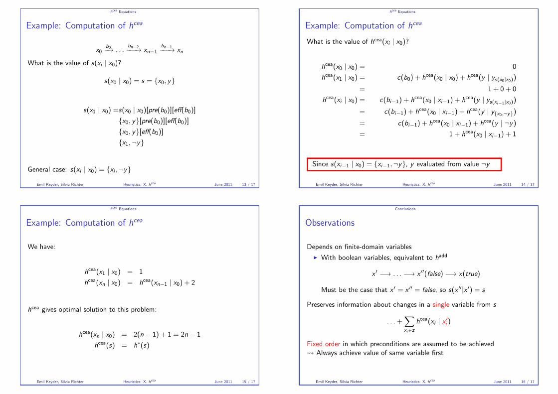
x0b0−→ . . .
bn−2−−−→ xn−1
bn−1−−−→ xn
What is the value of s(xi | x0)?
s(x0 | x0) = s = {x0, y}
s(x1 | x0) =s(x0 | x0)[pre(b0)][eff(b0)]{x0, y}[pre(b0)][eff(b0)]{x0, y}[eff(b0)]{x1,¬y}
General case: s(xi | x0) = {xi ,¬y}
Emil Keyder, Silvia Richter Heuristics: X. hcea June 2011 13 / 17
hcea Equations
Example: Computation of hcea
What is the value of hcea(xi | x0)?
hcea(x0 | x0) = 0
hcea(x1 | x0) = c(b0) + h
cea(x0 | x0) + hcea(y | ys(x0|x0))
= 1 + 0 + 0
hcea(xi | x0) = c(bi−1) + h
cea(x0 | xi−1) + hcea(y | ys(xi−1|x0))
= c(bi−1) + hcea(x0 | xi−1) + h
cea(y | y{x0,¬y})= c(bi−1) + h
cea(x0 | xi−1) + hcea(y | ¬y)
= 1 + hcea(x0 | xi−1) + 1
Since s(xi−1 | x0) = {xi−1,¬y}, y evaluated from value ¬y
Emil Keyder, Silvia Richter Heuristics: X. hcea June 2011 14 / 17
hcea Equations
Example: Computation of hcea
We have:
hcea(x1 | x0) = 1
hcea(xn | x0) = h
cea(xn−1 | x0) + 2
hcea gives optimal solution to this problem:
hcea(xn | x0) = 2(n − 1) + 1 = 2n − 1
hcea(s) = h
∗(s)
Emil Keyder, Silvia Richter Heuristics: X. hcea June 2011 15 / 17
Conclusions
Observations
Depends on finite-domain variables
� With boolean variables, equivalent to hadd
x� −→ . . . −→ x
��(false) −→ x(true)
Must be the case that x � = x �� = false, so s(x ��|x �) = s
Preserves information about changes in a single variable from s
. . .+�
xi∈zhcea(xi | x �i )
Fixed order in which preconditions are assumed to be achieved� Always achieve value of same variable first
Emil Keyder, Silvia Richter Heuristics: X. hcea June 2011 16 / 17
Conclusions
Conclusions
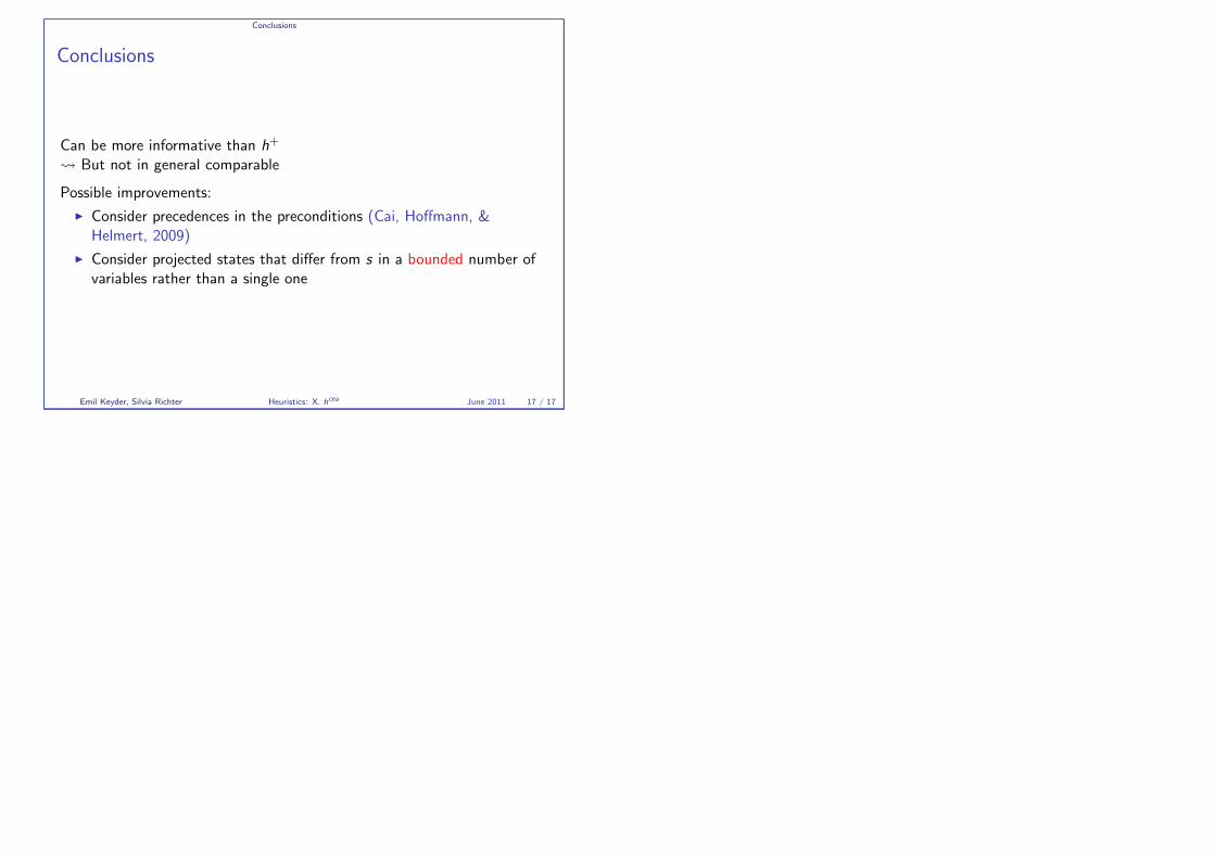
Can be more informative than h+
� But not in general comparable
Possible improvements:
� Consider precedences in the preconditions (Cai, Hoffmann, &Helmert, 2009)
� Consider projected states that differ from s in a bounded number ofvariables rather than a single one
Emil Keyder, Silvia Richter Heuristics: X. hcea June 2011 17 / 17
Heuristics for Domain-Independent Planning5. Landmark Heuristics
Emil Keyder Silvia Richter
Based partially on slides by Erez Karpas
ICAPS 2011 Summer School on Automated Planning and Scheduling
June 2011
Emil Keyder, Silvia Richter Heuristics: 5. Landmark Heuristics June 2011 1 / 52
What Landmarks AreLandmarksLandmark OrderingsComplexity
Landmark DiscoveryTheoryBackchainingForward Propagation & Declarative CharacterizationΠm LandmarksOrderings
Landmark-Counting HeuristicsThe LAMA Heuristic h
LM
The Admissible Landmark Heuristic hLA
The Landmark Cut HeuristicIdeaExample
Emil Keyder, Silvia Richter Heuristics: 5. Landmark Heuristics June 2011 2 / 52
What Landmarks Are Landmarks
Landmarks
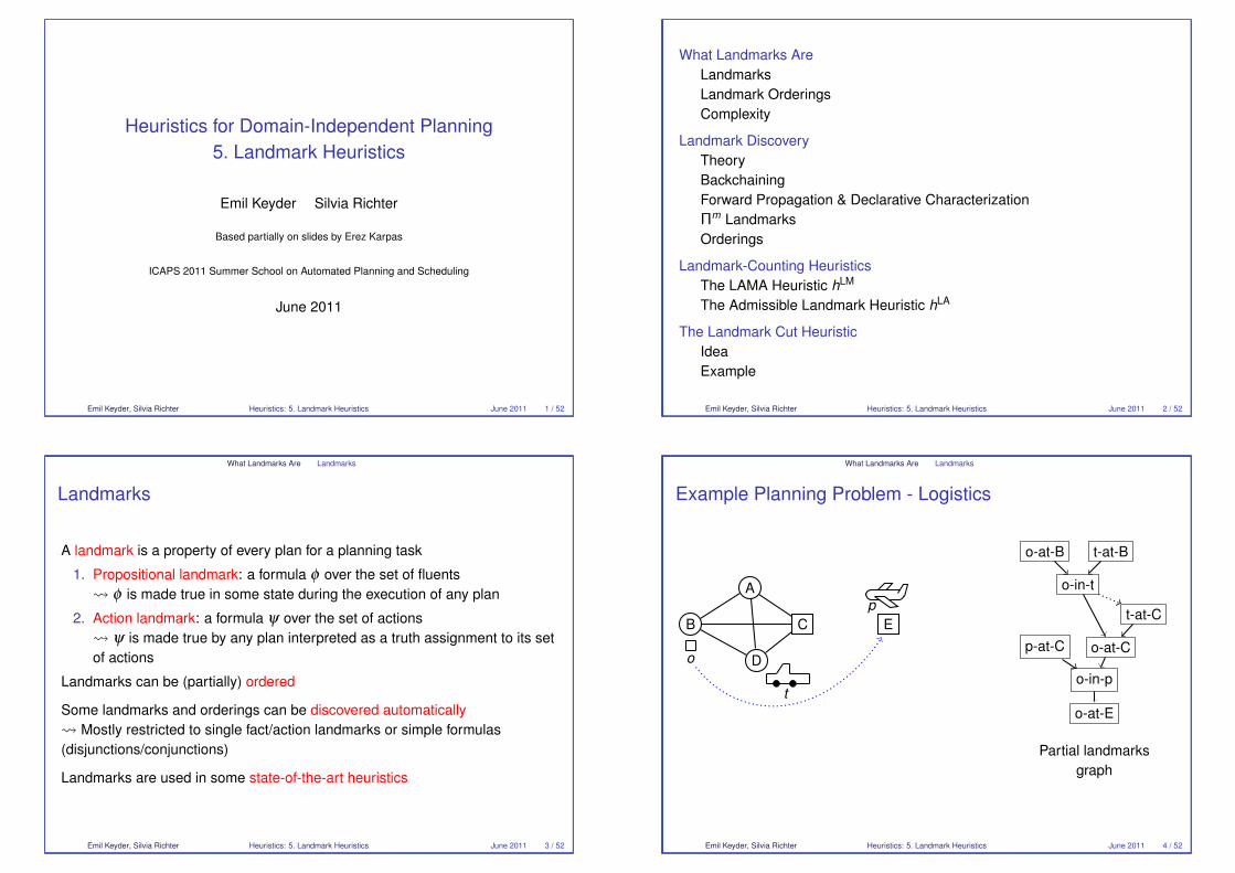
A landmark is a property of every plan for a planning task
1. Propositional landmark: a formula φ over the set of fluents� φ is made true in some state during the execution of any plan
2. Action landmark: a formula ψ over the set of actions� ψ is made true by any plan interpreted as a truth assignment to its setof actions
Landmarks can be (partially) ordered
Some landmarks and orderings can be discovered automatically� Mostly restricted to single fact/action landmarks or simple formulas(disjunctions/conjunctions)
Landmarks are used in some state-of-the-art heuristics
Emil Keyder, Silvia Richter Heuristics: 5. Landmark Heuristics June 2011 3 / 52
What Landmarks Are Landmarks
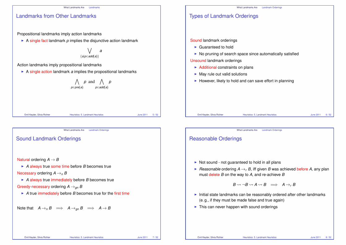
Example Planning Problem - Logistics
A
B C
Do
t
Ep
o-at-B
o-in-t
o-at-E
t-at-B
t-at-C
o-at-Cp-at-C
o-in-p
Partial landmarksgraph
Emil Keyder, Silvia Richter Heuristics: 5. Landmark Heuristics June 2011 4 / 52
What Landmarks Are Landmarks
Landmarks from Other Landmarks
Propositional landmarks imply action landmarks� A single fact landmark p implies the disjunctive action landmark
�
{a|p∈add(a)}a
Action landmarks imply propositional landmarks� A single action landmark a implies the propositional landmarks
�
p∈pre(a)
p and�
p∈add(a)
p
Emil Keyder, Silvia Richter Heuristics: 5. Landmark Heuristics June 2011 5 / 52
What Landmarks Are Landmark Orderings
Types of Landmark Orderings
Sound landmark orderings� Guaranteed to hold� No pruning of search space since automatically satisfied
Unsound landmark orderings� Additional constraints on plans� May rule out valid solutions� However, likely to hold and can save effort in planning
Emil Keyder, Silvia Richter Heuristics: 5. Landmark Heuristics June 2011 6 / 52
What Landmarks Are Landmark Orderings
Sound Landmark Orderings
Natural ordering A → B
� A always true some time before B becomes true
Necessary ordering A →n B
� A always true immediately before B becomes true
Greedy-necessary ordering A →gn B
� A true immediately before B becomes true for the first time
Note that A →n B =⇒ A →gn B =⇒ A → B
Emil Keyder, Silvia Richter Heuristics: 5. Landmark Heuristics June 2011 7 / 52
What Landmarks Are Landmark Orderings
Reasonable Orderings
� Not sound - not guaranteed to hold in all plans� Reasonable ordering A →r B, iff given B was achieved before A, any plan
must delete B on the way to A, and re-achieve B
B � ¬B � A � B =⇒ A →r B
� Initial state landmarks can be reasonably ordered after other landmarks(e. g., if they must be made false and true again)
� This can never happen with sound orderings
Emil Keyder, Silvia Richter Heuristics: 5. Landmark Heuristics June 2011 8 / 52
What Landmarks Are Complexity
Landmark Complexity
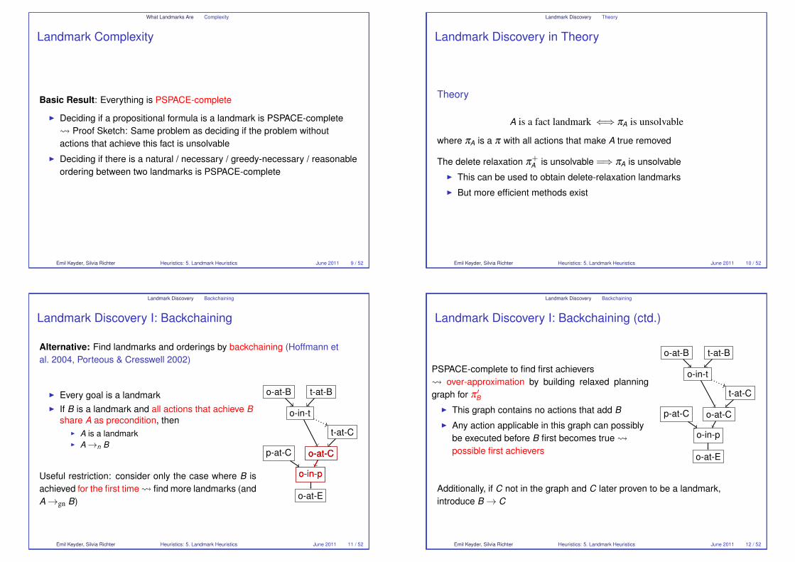
Basic Result: Everything is PSPACE-complete
� Deciding if a propositional formula is a landmark is PSPACE-complete� Proof Sketch: Same problem as deciding if the problem withoutactions that achieve this fact is unsolvable
� Deciding if there is a natural / necessary / greedy-necessary / reasonableordering between two landmarks is PSPACE-complete
Emil Keyder, Silvia Richter Heuristics: 5. Landmark Heuristics June 2011 9 / 52
Landmark Discovery Theory
Landmark Discovery in Theory
Theory
A is a fact landmark ⇐⇒ πA is unsolvable
where πA is a π with all actions that make A true removed
The delete relaxation π+A
is unsolvable =⇒ πA is unsolvable� This can be used to obtain delete-relaxation landmarks� But more efficient methods exist
Emil Keyder, Silvia Richter Heuristics: 5. Landmark Heuristics June 2011 10 / 52
Landmark Discovery Backchaining
Landmark Discovery I: Backchaining
Alternative: Find landmarks and orderings by backchaining (Hoffmann etal. 2004, Porteous & Cresswell 2002)
� Every goal is a landmark� If B is a landmark and all actions that achieve B
share A as precondition, then� A is a landmark� A →n B
Useful restriction: consider only the case where B isachieved for the first time � find more landmarks (andA →gn B)
o-at-B
o-in-t
o-at-E
t-at-B
t-at-C
o-at-Co-at-Cp-at-C
o-in-po-in-p
Emil Keyder, Silvia Richter Heuristics: 5. Landmark Heuristics June 2011 11 / 52
Landmark Discovery Backchaining
Landmark Discovery I: Backchaining (ctd.)
PSPACE-complete to find first achievers� over-approximation by building relaxed planninggraph for π �
B
� This graph contains no actions that add B
� Any action applicable in this graph can possiblybe executed before B first becomes true �possible first achievers
o-at-B
o-in-t
o-at-E
t-at-B
t-at-C
o-at-Cp-at-C
o-in-p
Additionally, if C not in the graph and C later proven to be a landmark,introduce B → C
Emil Keyder, Silvia Richter Heuristics: 5. Landmark Heuristics June 2011 12 / 52
Landmark Discovery Backchaining
Landmark Discovery I: Backchaining (ctd.)
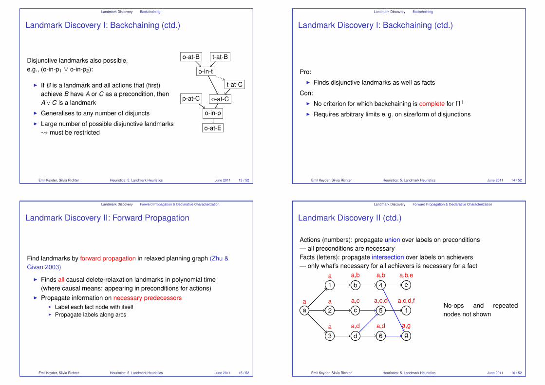
Disjunctive landmarks also possible,e.g., (o-in-p1 ∨ o-in-p2):
� If B is a landmark and all actions that (first)achieve B have A or C as a precondition, thenA∨C is a landmark
� Generalises to any number of disjuncts� Large number of possible disjunctive landmarks
� must be restricted
o-at-B
o-in-t
o-at-E
t-at-B
t-at-C
o-at-Cp-at-C
o-in-p
Emil Keyder, Silvia Richter Heuristics: 5. Landmark Heuristics June 2011 13 / 52
Landmark Discovery Backchaining
Landmark Discovery I: Backchaining (ctd.)
Pro:� Finds disjunctive landmarks as well as facts
Con:� No criterion for which backchaining is complete for Π+
� Requires arbitrary limits e. g. on size/form of disjunctions
Emil Keyder, Silvia Richter Heuristics: 5. Landmark Heuristics June 2011 14 / 52
Landmark Discovery Forward Propagation & Declarative Characterization
Landmark Discovery II: Forward Propagation
Find landmarks by forward propagation in relaxed planning graph (Zhu &Givan 2003)
� Finds all causal delete-relaxation landmarks in polynomial time(where causal means: appearing in preconditions for actions)
� Propagate information on necessary predecessors� Label each fact node with itself� Propagate labels along arcs
Emil Keyder, Silvia Richter Heuristics: 5. Landmark Heuristics June 2011 15 / 52
Landmark Discovery Forward Propagation & Declarative Characterization
Landmark Discovery II (ctd.)
Actions (numbers): propagate union over labels on preconditions— all preconditions are necessaryFacts (letters): propagate intersection over labels on achievers— only what’s necessary for all achievers is necessary for a fact
aa
1
2
3
a
a
a
b
c
d
a,b
a,c
a,d
4
5
6
a,b
a,c,d
a,d
e
f
g
a,b,e
a,c,d,f
a,g
No-ops and repeatednodes not shown
Emil Keyder, Silvia Richter Heuristics: 5. Landmark Heuristics June 2011 16 / 52
Landmark Discovery Forward Propagation & Declarative Characterization
Landmark Discovery II (ctd.)
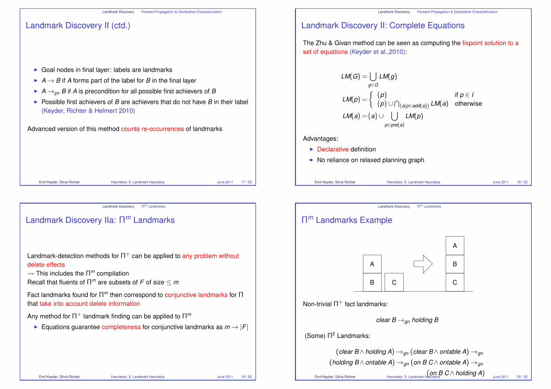
� Goal nodes in final layer: labels are landmarks� A → B if A forms part of the label for B in the final layer� A →gn B if A is precondition for all possible first achievers of B
� Possible first achievers of B are achievers that do not have B in their label(Keyder, Richter & Helmert 2010)
Advanced version of this method counts re-occurrences of landmarks
Emil Keyder, Silvia Richter Heuristics: 5. Landmark Heuristics June 2011 17 / 52
Landmark Discovery Forward Propagation & Declarative Characterization
Landmark Discovery II: Complete Equations
The Zhu & Givan method can be seen as computing the fixpoint solution to aset of equations (Keyder et al.,2010):
LM(G) =�
g∈G
LM(g)
LM(p) =
�{p} if p ∈ I
{p}∪�
{a|p∈add(a)} LM(a) otherwise
LM(a) ={a}∪�
p∈pre(a)
LM(p)
Advantages:� Declarative definition� No reliance on relaxed planning graph
Emil Keyder, Silvia Richter Heuristics: 5. Landmark Heuristics June 2011 18 / 52
Landmark Discovery Πm Landmarks
Landmark Discovery IIa: Πm Landmarks
Landmark-detection methods for Π+ can be applied to any problem withoutdelete effects� This includes the Πm compilationRecall that fluents of Πm are subsets of F of size ≤ m
Fact landmarks found for Πm then correspond to conjunctive landmarks for Πthat take into account delete information
Any method for Π+ landmark finding can be applied to Πm
� Equations guarantee completeness for conjunctive landmarks as m → |F |
Emil Keyder, Silvia Richter Heuristics: 5. Landmark Heuristics June 2011 19 / 52
Landmark Discovery Πm Landmarks
Πm Landmarks Example
A
B C
A
B
C
Non-trivial Π+ fact landmarks:
clear B →gn holding B
(Some) Π2 Landmarks:
(clear B∧holding A)→gn (clear B∧ontable A)→gn
(holding B∧ontable A)→gn (on B C∧ontable A)→gn
(on B C∧holding A)Emil Keyder, Silvia Richter Heuristics: 5. Landmark Heuristics June 2011 20 / 52
Landmark Discovery Orderings
Finding Orderings
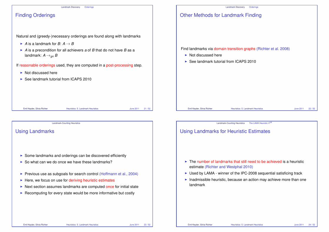
Natural and (greedy-)necessary orderings are found along with landmarks
� A is a landmark for B: A → B
� A is a precondition for all achievers a of B that do not have B as alandmark: A →gn B
If reasonable orderings used, they are computed in a post-processing step.
� Not discussed here� See landmark tutorial from ICAPS 2010
Emil Keyder, Silvia Richter Heuristics: 5. Landmark Heuristics June 2011 21 / 52
Landmark Discovery Orderings
Other Methods for Landmark Finding
Find landmarks via domain transition graphs (Richter et al. 2008)� Not discussed here� See landmark tutorial from ICAPS 2010
Emil Keyder, Silvia Richter Heuristics: 5. Landmark Heuristics June 2011 22 / 52
Landmark-Counting Heuristics
Using Landmarks
� Some landmarks and orderings can be discovered efficiently� So what can we do once we have these landmarks?
� Previous use as subgoals for search control (Hoffmann et al., 2004)� Here, we focus on use for deriving heuristic estimates� Next section assumes landmarks are computed once for initial state� Recomputing for every state would be more informative but costly
Emil Keyder, Silvia Richter Heuristics: 5. Landmark Heuristics June 2011 23 / 52
Landmark-Counting Heuristics The LAMA Heuristic hLM
Using Landmarks for Heuristic Estimates
� The number of landmarks that still need to be achieved is a heuristicestimate (Richter and Westphal 2010)
� Used by LAMA - winner of the IPC-2008 sequential satisficing track� Inadmissible heuristic, because an action may achieve more than one
landmark
Emil Keyder, Silvia Richter Heuristics: 5. Landmark Heuristics June 2011 24 / 52
Landmark-Counting Heuristics The LAMA Heuristic hLM
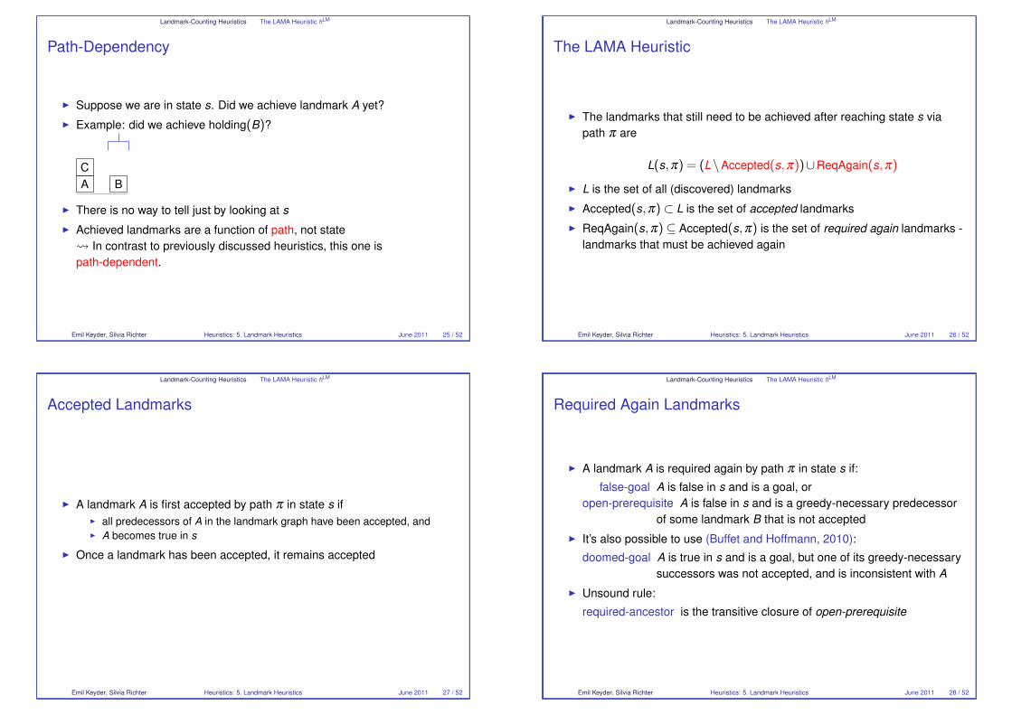
Path-Dependency
� Suppose we are in state s. Did we achieve landmark A yet?� Example: did we achieve holding(B)?
AC
B
� There is no way to tell just by looking at s
� Achieved landmarks are a function of path, not state� In contrast to previously discussed heuristics, this one ispath-dependent.
Emil Keyder, Silvia Richter Heuristics: 5. Landmark Heuristics June 2011 25 / 52
Landmark-Counting Heuristics The LAMA Heuristic hLM
The LAMA Heuristic
� The landmarks that still need to be achieved after reaching state s viapath π are
L(s,π) = (L\Accepted(s,π))∪ReqAgain(s,π)
� L is the set of all (discovered) landmarks� Accepted(s,π)⊂ L is the set of accepted landmarks� ReqAgain(s,π)⊆ Accepted(s,π) is the set of required again landmarks -
landmarks that must be achieved again
Emil Keyder, Silvia Richter Heuristics: 5. Landmark Heuristics June 2011 26 / 52
Landmark-Counting Heuristics The LAMA Heuristic hLM
Accepted Landmarks
� A landmark A is first accepted by path π in state s if� all predecessors of A in the landmark graph have been accepted, and� A becomes true in s
� Once a landmark has been accepted, it remains accepted
Emil Keyder, Silvia Richter Heuristics: 5. Landmark Heuristics June 2011 27 / 52
Landmark-Counting Heuristics The LAMA Heuristic hLM
Required Again Landmarks
� A landmark A is required again by path π in state s if:false-goal A is false in s and is a goal, or
open-prerequisite A is false in s and is a greedy-necessary predecessorof some landmark B that is not accepted
� It’s also possible to use (Buffet and Hoffmann, 2010):doomed-goal A is true in s and is a goal, but one of its greedy-necessary
successors was not accepted, and is inconsistent with A
� Unsound rule:required-ancestor is the transitive closure of open-prerequisite
Emil Keyder, Silvia Richter Heuristics: 5. Landmark Heuristics June 2011 28 / 52
Landmark-Counting Heuristics The LAMA Heuristic hLM
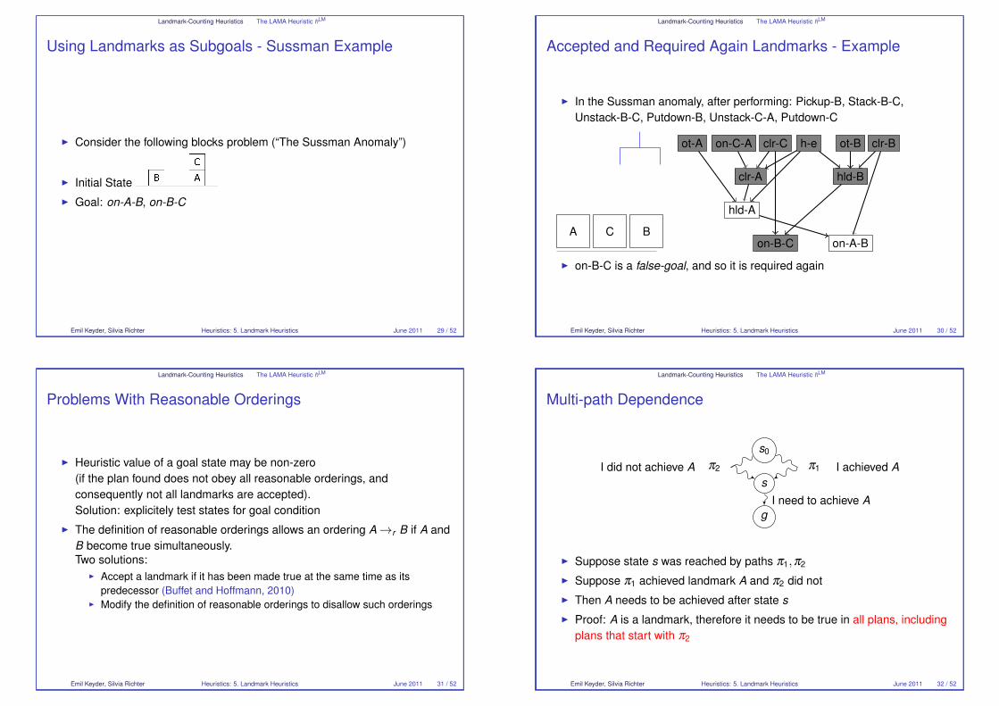
Using Landmarks as Subgoals - Sussman Example
� Consider the following blocks problem (“The Sussman Anomaly”)
� Initial State� Goal: on-A-B, on-B-C
Emil Keyder, Silvia Richter Heuristics: 5. Landmark Heuristics June 2011 29 / 52
Landmark-Counting Heuristics The LAMA Heuristic hLM
Accepted and Required Again Landmarks - Example
� In the Sussman anomaly, after performing: Pickup-B, Stack-B-C,Unstack-B-C, Putdown-B, Unstack-C-A, Putdown-C
A C B
ot-A on-C-A clr-C h-e ot-B clr-B
clr-A hld-B
hld-A
on-B-C on-A-B
� on-B-C is a false-goal, and so it is required again
Emil Keyder, Silvia Richter Heuristics: 5. Landmark Heuristics June 2011 30 / 52
Landmark-Counting Heuristics The LAMA Heuristic hLM
Problems With Reasonable Orderings
� Heuristic value of a goal state may be non-zero(if the plan found does not obey all reasonable orderings, andconsequently not all landmarks are accepted).Solution: explicitely test states for goal condition
� The definition of reasonable orderings allows an ordering A →r B if A andB become true simultaneously.Two solutions:
� Accept a landmark if it has been made true at the same time as itspredecessor (Buffet and Hoffmann, 2010)
� Modify the definition of reasonable orderings to disallow such orderings
Emil Keyder, Silvia Richter Heuristics: 5. Landmark Heuristics June 2011 31 / 52
Landmark-Counting Heuristics The LAMA Heuristic hLM
Multi-path Dependence
s0
s
g
π1π2 I achieved AI did not achieve A
I need to achieve A
� Suppose state s was reached by paths π1,π2
� Suppose π1 achieved landmark A and π2 did not� Then A needs to be achieved after state s
� Proof: A is a landmark, therefore it needs to be true in all plans, includingplans that start with π2
Emil Keyder, Silvia Richter Heuristics: 5. Landmark Heuristics June 2011 32 / 52
Landmark-Counting Heuristics The LAMA Heuristic hLM
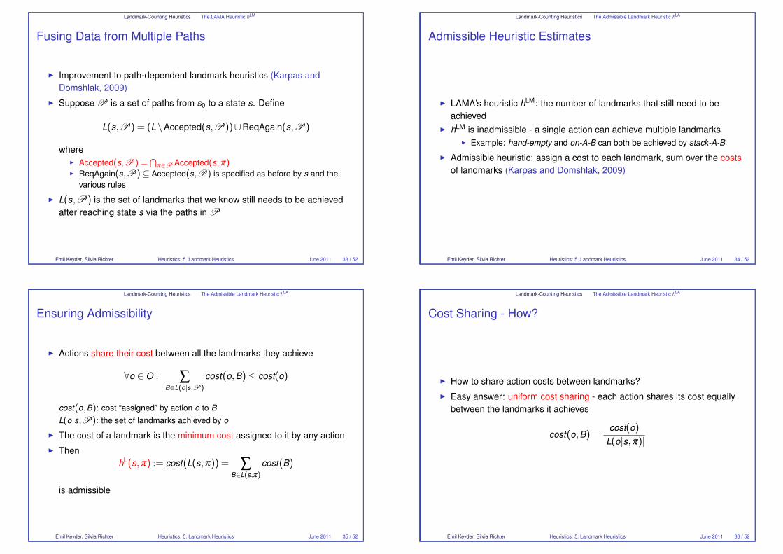
Fusing Data from Multiple Paths
� Improvement to path-dependent landmark heuristics (Karpas andDomshlak, 2009)
� Suppose P is a set of paths from s0 to a state s. Define
L(s,P) = (L\Accepted(s,P))∪ReqAgain(s,P)
where� Accepted(s,P) =
�π∈P Accepted(s,π)
� ReqAgain(s,P)⊆ Accepted(s,P) is specified as before by s and thevarious rules
� L(s,P) is the set of landmarks that we know still needs to be achievedafter reaching state s via the paths in P
Emil Keyder, Silvia Richter Heuristics: 5. Landmark Heuristics June 2011 33 / 52
Landmark-Counting Heuristics The Admissible Landmark Heuristic hLA
Admissible Heuristic Estimates
� LAMA’s heuristic hLM: the number of landmarks that still need to be
achieved� h
LM is inadmissible - a single action can achieve multiple landmarks� Example: hand-empty and on-A-B can both be achieved by stack-A-B
� Admissible heuristic: assign a cost to each landmark, sum over the costsof landmarks (Karpas and Domshlak, 2009)
Emil Keyder, Silvia Richter Heuristics: 5. Landmark Heuristics June 2011 34 / 52
Landmark-Counting Heuristics The Admissible Landmark Heuristic hLA
Ensuring Admissibility
� Actions share their cost between all the landmarks they achieve
∀o ∈ O : ∑B∈L(o|s,P)
cost(o,B)≤ cost(o)
cost(o,B): cost “assigned” by action o to B
L(o|s,P): the set of landmarks achieved by o
� The cost of a landmark is the minimum cost assigned to it by any action� Then
hL(s,π) := cost(L(s,π)) = ∑
B∈L(s,π)cost(B)
is admissible
Emil Keyder, Silvia Richter Heuristics: 5. Landmark Heuristics June 2011 35 / 52
Landmark-Counting Heuristics The Admissible Landmark Heuristic hLA
Cost Sharing - How?
� How to share action costs between landmarks?� Easy answer: uniform cost sharing - each action shares its cost equally
between the landmarks it achieves
cost(o,B) =cost(o)
|L(o|s,π)|
Emil Keyder, Silvia Richter Heuristics: 5. Landmark Heuristics June 2011 36 / 52

Landmark-Counting Heuristics The Admissible Landmark Heuristic hLA
Uniform Cost Sharing
� Advantage: Easy and fast to compute� Disadvantage: can be much worse than the optimal cost partitioning
� Example: all actions cost 1 – uniform cost sharing
q
p1
p2
p3
p4
a1
a2
a3
a4
0.5
0.50.5
0.5
0.5
0.5
0.5
0.5
min(0.5,0.5,0.5,0.5)=0.5
min(0.5)=0.5
min(0.5)=0.5
min(0.5)=0.5
min(0.5)=0.5
hL = 2.5
uniform hL = 2.5
0
10
1
0
1
0
1
min(0,0,0,0)=0
min(1)=1
min(1)=1
min(1)=1
min(1)=1
hL = 4
Emil Keyder, Silvia Richter Heuristics: 5. Landmark Heuristics June 2011 37 / 52
Landmark-Counting Heuristics The Admissible Landmark Heuristic hLA
Uniform Cost Sharing
� Advantage: Easy and fast to compute� Disadvantage: can be much worse than the optimal cost partitioning
� Example: all actions cost 1 – optimal cost sharing
q
p1
p2
p3
p4
a1
a2
a3
a4
0.5
0.50.5
0.5
0.5
0.5
0.5
0.5
min(0.5,0.5,0.5,0.5)=0.5
min(0.5)=0.5
min(0.5)=0.5
min(0.5)=0.5
min(0.5)=0.5
hL = 2.5
uniform hL = 2.5
0
10
1
0
1
0
1
min(0,0,0,0)=0
min(1)=1
min(1)=1
min(1)=1
min(1)=1
hL = 4
Emil Keyder, Silvia Richter Heuristics: 5. Landmark Heuristics June 2011 38 / 52
Landmark-Counting Heuristics The Admissible Landmark Heuristic hLA
Optimal Cost Sharing
� The good news: the optimal cost partitioning is poly-time to compute� The constraints for admissibility are linear, and can be used in a Linear
Program (LP)� Objective: maximize the sum of landmark costs� The solution to the LP gives us the optimal cost partitioning
� The bad news: poly-time can still take a long time
Emil Keyder, Silvia Richter Heuristics: 5. Landmark Heuristics June 2011 39 / 52
Landmark-Counting Heuristics The Admissible Landmark Heuristic hLA
How can we do better?
So far:� Uniform cost sharing is easy to compute, but suboptimal� Optimal cost sharing takes a long time to compute
Q: How can we get better heuristic estimates that don’t take a long time tocompute?
A: Exploit additional information - action landmarks
Emil Keyder, Silvia Richter Heuristics: 5. Landmark Heuristics June 2011 40 / 52

Landmark-Counting Heuristics The Admissible Landmark Heuristic hLA
Using Action Landmarks - by Example
q
p1
p2
p3
p4
a1
a2
a3
a4
p2
p3
p4
a1
a2
a3
a4
1
1
1
1
Uniform Cost Sharing
min(1)=1
min(1)=1
min(1)=1
hLA = 4
Emil Keyder, Silvia Richter Heuristics: 5. Landmark Heuristics June 2011 41 / 52
Landmark-Counting Heuristics The Admissible Landmark Heuristic hLA
Summary
� Landmarks describe the implicit structure of a planning task� Can be used to derive admissible and inadmissible landmark-counting
heuristics� These heuristics are path-dependent
Emil Keyder, Silvia Richter Heuristics: 5. Landmark Heuristics June 2011 42 / 52
The Landmark Cut Heuristic Idea
The Landmark Cut Heuristic
A landmark heuristic that is not path-dependent
� Computes landmarks for each state rather than once� New way of finding landmarks� Very accurate admissible approximation of h
+
Emil Keyder, Silvia Richter Heuristics: 5. Landmark Heuristics June 2011 43 / 52
The Landmark Cut Heuristic Idea
The Landmark Cut Heuristic (cont.)
Idea (Helmert & Domshlak, 2009):� Use critical paths (from h
max computation) to find disjunctive actionlandmarks
� Extract landmarks iteratively, subtracting their cost from hmax estimates
� Cost of each landmark := cost of cheapest action in landmark� Heuristic value := sum over all landmark costs
Emil Keyder, Silvia Richter Heuristics: 5. Landmark Heuristics June 2011 44 / 52
The Landmark Cut Heuristic Idea
The Landmark Cut Heuristic (cont.)
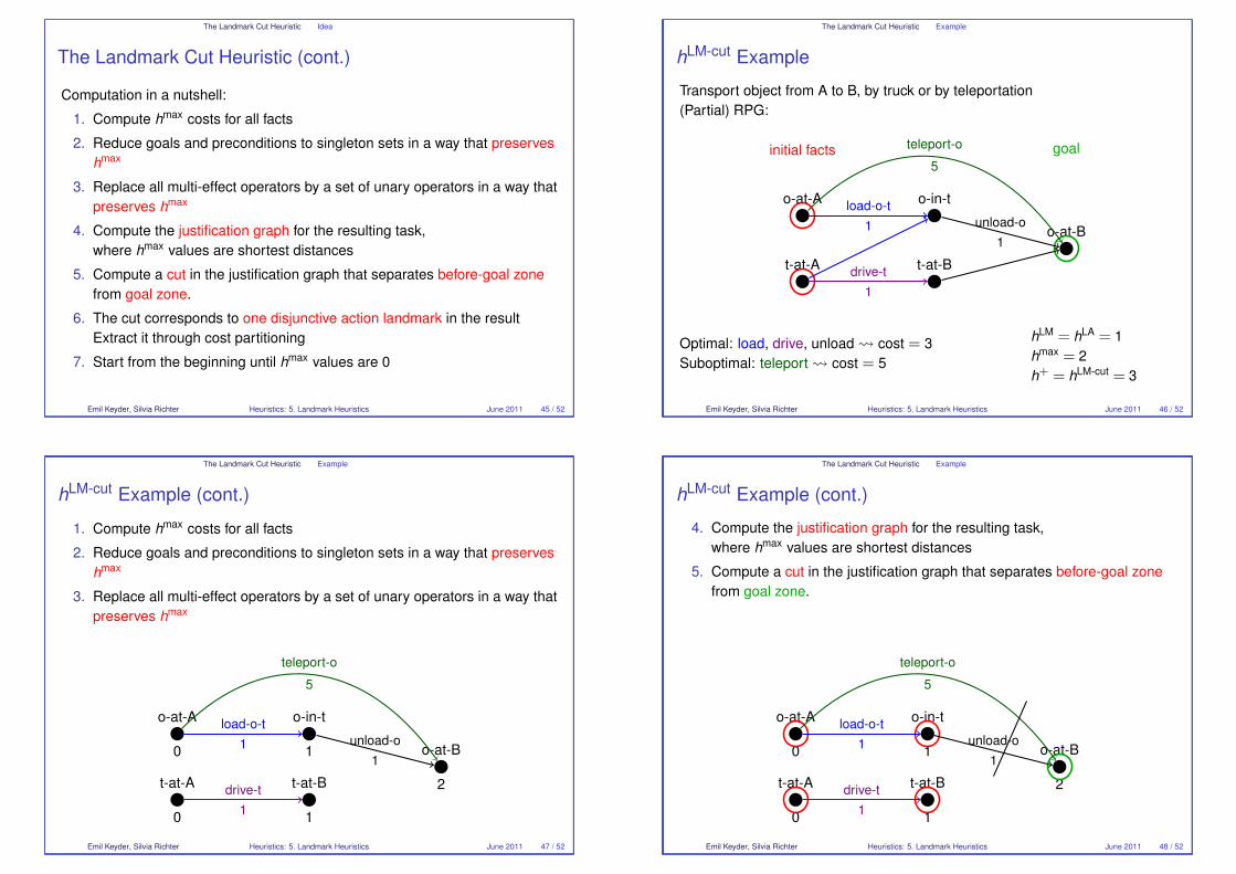
Computation in a nutshell:
1. Compute hmax costs for all facts
2. Reduce goals and preconditions to singleton sets in a way that preservesh
max
3. Replace all multi-effect operators by a set of unary operators in a way thatpreserves h
max
4. Compute the justification graph for the resulting task,where h
max values are shortest distances
5. Compute a cut in the justification graph that separates before-goal zonefrom goal zone.
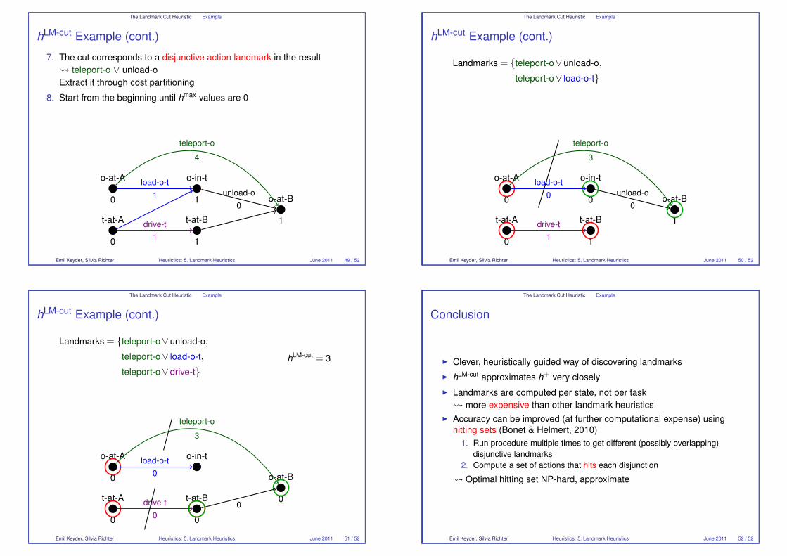
6. The cut corresponds to one disjunctive action landmark in the resultExtract it through cost partitioning
7. Start from the beginning until hmax values are 0
Emil Keyder, Silvia Richter Heuristics: 5. Landmark Heuristics June 2011 45 / 52
The Landmark Cut Heuristic Example
hLM-cut Example
Transport object from A to B, by truck or by teleportation(Partial) RPG:
initial facts goal
o-at-A
t-at-A
o-in-t
t-at-B
o-at-B
load-o-t1
drive-t1
unload-o1
teleport-o
5
Optimal: load, drive, unload � cost = 3Suboptimal: teleport � cost = 5
hLM = h
LA = 1h
max = 2h+ = h
LM-cut = 3
Emil Keyder, Silvia Richter Heuristics: 5. Landmark Heuristics June 2011 46 / 52
The Landmark Cut Heuristic Example
hLM-cut Example (cont.)
1. Compute hmax costs for all facts
2. Reduce goals and preconditions to singleton sets in a way that preservesh
max
3. Replace all multi-effect operators by a set of unary operators in a way thatpreserves h
max
o-at-A
0
t-at-A
0
o-in-t
1
t-at-B
1
o-at-B
2
load-o-t1
drive-t1
unload-o1
teleport-o
5
Emil Keyder, Silvia Richter Heuristics: 5. Landmark Heuristics June 2011 47 / 52
The Landmark Cut Heuristic Example
hLM-cut Example (cont.)
4. Compute the justification graph for the resulting task,where h
max values are shortest distances
5. Compute a cut in the justification graph that separates before-goal zonefrom goal zone.
o-at-A
0
t-at-A
0
o-in-t
1
t-at-B
1
o-at-B
2
load-o-t1
drive-t1
unload-o1
teleport-o
5
Emil Keyder, Silvia Richter Heuristics: 5. Landmark Heuristics June 2011 48 / 52
The Landmark Cut Heuristic Example
hLM-cut Example (cont.)
7. The cut corresponds to a disjunctive action landmark in the result� teleport-o ∨ unload-oExtract it through cost partitioning
8. Start from the beginning until hmax values are 0
o-at-A
0
t-at-A
0
o-in-t
1
t-at-B
1
o-at-B
1
load-o-t1
drive-t1
unload-o0
teleport-o
4
Emil Keyder, Silvia Richter Heuristics: 5. Landmark Heuristics June 2011 49 / 52
The Landmark Cut Heuristic Example
hLM-cut Example (cont.)
Landmarks = {teleport-o∨unload-o,
teleport-o∨ load-o-t}
,
teleport-o∨drive-t}h
LM-cut = 3
o-at-A
0
t-at-A
0
o-in-t
0
t-at-B
1
o-at-B
1
load-o-t0
drive-t1
unload-o0
0
teleport-o
3
Emil Keyder, Silvia Richter Heuristics: 5. Landmark Heuristics June 2011 50 / 52
The Landmark Cut Heuristic Example
hLM-cut Example (cont.)
Landmarks = {teleport-o∨unload-o,
teleport-o∨ load-o-t,
teleport-o∨drive-t}h
LM-cut = 3
o-at-A
0
t-at-A
0
o-in-t
t-at-B
0
o-at-B
0
load-o-t0
drive-t0
unload-o0
0
teleport-o
3
Emil Keyder, Silvia Richter Heuristics: 5. Landmark Heuristics June 2011 51 / 52
The Landmark Cut Heuristic Example
Conclusion
� Clever, heuristically guided way of discovering landmarks� h
LM-cut approximates h+ very closely
� Landmarks are computed per state, not per task� more expensive than other landmark heuristics
� Accuracy can be improved (at further computational expense) usinghitting sets (Bonet & Helmert, 2010)
1. Run procedure multiple times to get different (possibly overlapping)disjunctive landmarks
2. Compute a set of actions that hits each disjunction
� Optimal hitting set NP-hard, approximate
Emil Keyder, Silvia Richter Heuristics: 5. Landmark Heuristics June 2011 52 / 52
Heuristics for Domain-Independent Planning6. Abstraction Heuristics
Emil Keyder Silvia Richter
Based on slides by Carmel Domshlak and Malte Helmert
ICAPS 2011 Summer School on Automated Planning and Scheduling
June 2011
Emil Keyder, Silvia Richter Heuristics: 6. Abstraction Heuristics June 2011 1 / 36
IntroductionTransition SystemsAbstractions
Pattern Database HeuristicsIntroductionExamplesMultiple & Additive PatternsFinding Good Patterns
Merge-and-Shrink HeuristicsIntroductionMergingShrinkingGeneric AlgorithmTheoretical Properties
Structural Pattern Heuristics
Emil Keyder, Silvia Richter Heuristics: 6. Abstraction Heuristics June 2011 2 / 36
Introduction Transition Systems
Motivation
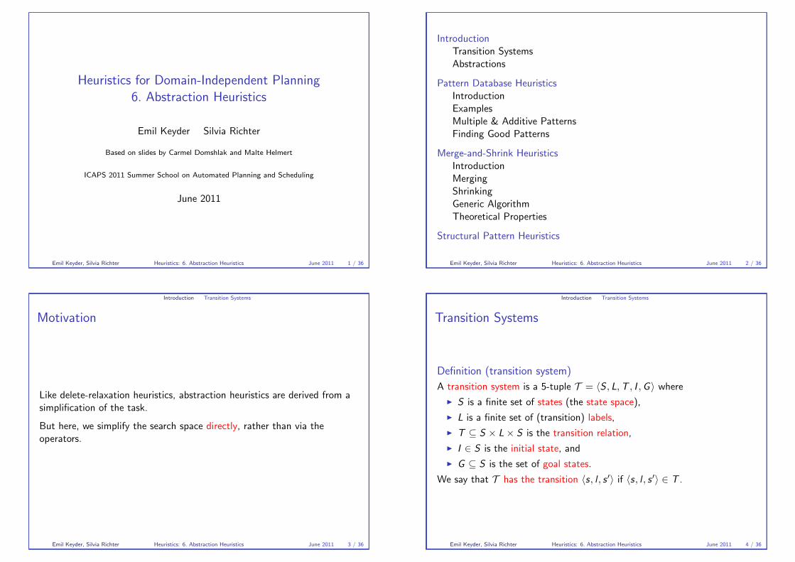
Like delete-relaxation heuristics, abstraction heuristics are derived from asimplification of the task.
But here, we simplify the search space directly, rather than via theoperators.
Emil Keyder, Silvia Richter Heuristics: 6. Abstraction Heuristics June 2011 3 / 36
Introduction Transition Systems
Transition Systems
Definition (transition system)
A transition system is a 5-tuple T = �S , L,T , I ,G � where� S is a finite set of states (the state space),
� L is a finite set of (transition) labels,
� T ⊆ S × L× S is the transition relation,
� I ∈ S is the initial state, and
� G ⊆ S is the set of goal states.
We say that T has the transition �s, l , s �� if �s, l , s �� ∈ T .
Emil Keyder, Silvia Richter Heuristics: 6. Abstraction Heuristics June 2011 4 / 36
Introduction Transition Systems
Transition Systems of SAS+ Planning Tasks
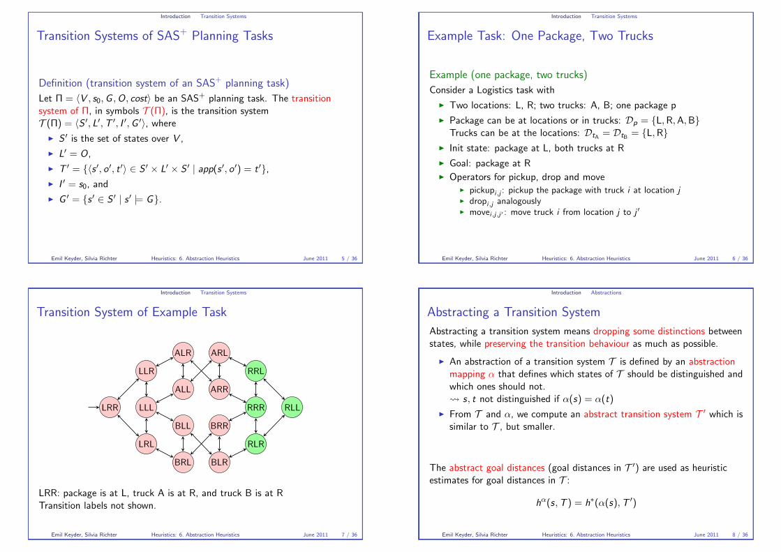
Definition (transition system of an SAS+ planning task)
Let Π = �V , s0,G ,O, cost� be an SAS+ planning task. The transitionsystem of Π, in symbols T (Π), is the transition systemT (Π) = �S �, L�,T �, I �,G ��, where
� S � is the set of states over V ,
� L� = O,
� T � = {�s �, o �, t �� ∈ S � × L� × S � | app(s �, o �) = t �},� I � = s0, and
� G � = {s � ∈ S � | s � |= G}.
Emil Keyder, Silvia Richter Heuristics: 6. Abstraction Heuristics June 2011 5 / 36
Introduction Transition Systems
Example Task: One Package, Two Trucks
Example (one package, two trucks)
Consider a Logistics task with
� Two locations: L, R; two trucks: A, B; one package p
� Package can be at locations or in trucks: Dp = {L,R,A,B}Trucks can be at the locations: DtA = DtB = {L,R}
� Init state: package at L, both trucks at R
� Goal: package at R� Operators for pickup, drop and move
� pickupi,j : pickup the package with truck i at location j
� dropi,j analogously� movei,j,j� : move truck i from location j to j �
Emil Keyder, Silvia Richter Heuristics: 6. Abstraction Heuristics June 2011 6 / 36
Introduction Transition Systems
Transition System of Example Task
LRR LLL
LLR
LRL
ALR
ALL
BLL
BRL
ARL
ARR
BRR
BLR
RRR
RRL
RLR
RLL
LRR: package is at L, truck A is at R, and truck B is at RTransition labels not shown.
Emil Keyder, Silvia Richter Heuristics: 6. Abstraction Heuristics June 2011 7 / 36
Introduction Abstractions
Abstracting a Transition System
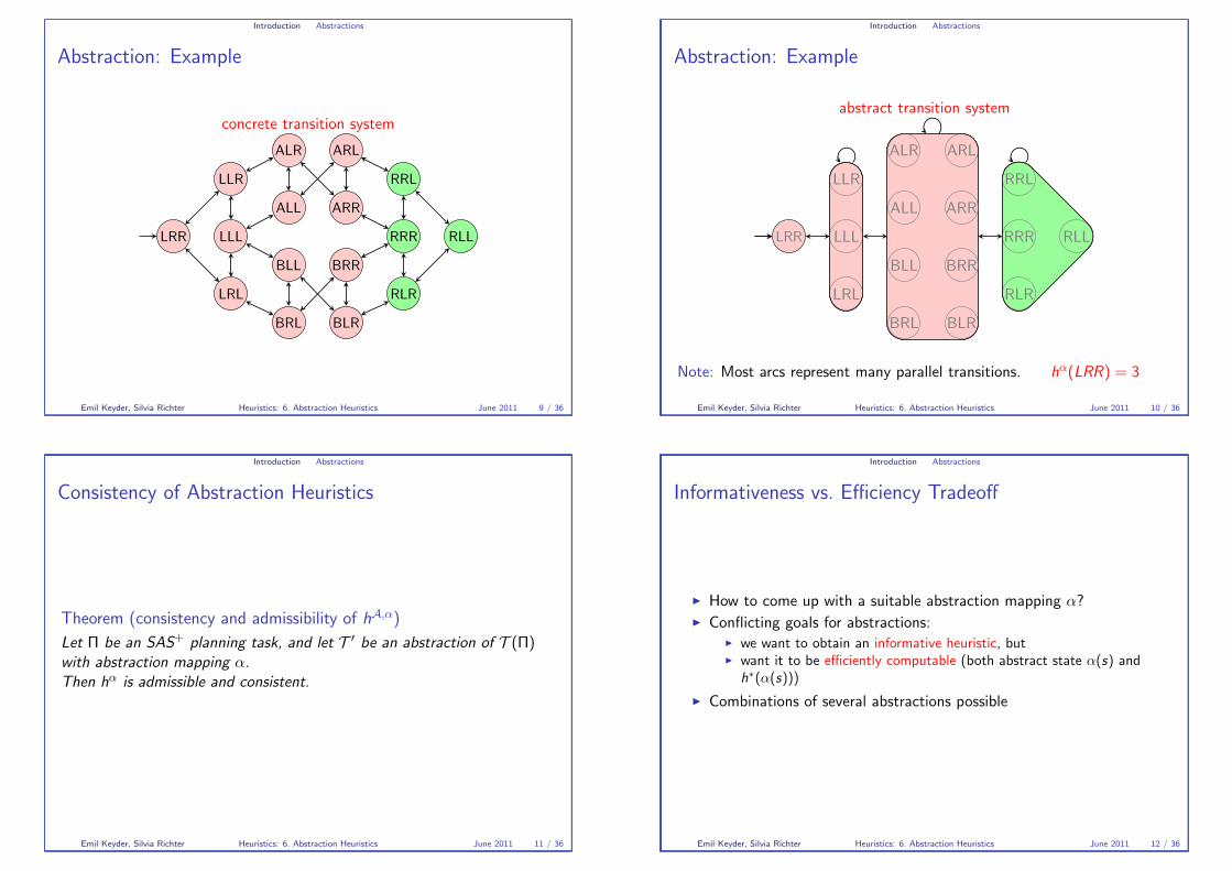
Abstracting a transition system means dropping some distinctions betweenstates, while preserving the transition behaviour as much as possible.
� An abstraction of a transition system T is defined by an abstractionmapping α that defines which states of T should be distinguished andwhich ones should not.� s, t not distinguished if α(s) = α(t)
� From T and α, we compute an abstract transition system T � which issimilar to T , but smaller.
The abstract goal distances (goal distances in T �) are used as heuristicestimates for goal distances in T :
hα(s,T ) = h
∗(α(s),T �)
Emil Keyder, Silvia Richter Heuristics: 6. Abstraction Heuristics June 2011 8 / 36
Introduction Abstractions
Abstraction: Example
concrete transition system
LRR LLL
LLR
LRL
ALR
ALL
BLL
BRL
ARL
ARR
BRR
BLR
RRR
RRL
RLR
RLL
Emil Keyder, Silvia Richter Heuristics: 6. Abstraction Heuristics June 2011 9 / 36
Introduction Abstractions
Abstraction: Example
abstract transition system
LRR
LLR
LLL
LRL
LLR
LRL
LLL
ALR ARL
ALL ARR
BLL
BRL
BRR
BLR
ALR ARL
BLRBRL
ALL ARR
BLL BRR
RRR
RRL
RLR
RLLRLL
RRL
RLR
RRR
Note: Most arcs represent many parallel transitions. hα(LRR) = 3
Emil Keyder, Silvia Richter Heuristics: 6. Abstraction Heuristics June 2011 10 / 36
Introduction Abstractions
Consistency of Abstraction Heuristics
Theorem (consistency and admissibility of hA,α)
Let Π be an SAS+planning task, and let T � be an abstraction of T (Π)
with abstraction mapping α.Then hα is admissible and consistent.
Emil Keyder, Silvia Richter Heuristics: 6. Abstraction Heuristics June 2011 11 / 36
Introduction Abstractions
Informativeness vs. Efficiency Tradeoff
� How to come up with a suitable abstraction mapping α?� Conflicting goals for abstractions:
� we want to obtain an informative heuristic, but� want it to be efficiently computable (both abstract state α(s) and
h∗(α(s)))
� Combinations of several abstractions possible
Emil Keyder, Silvia Richter Heuristics: 6. Abstraction Heuristics June 2011 12 / 36
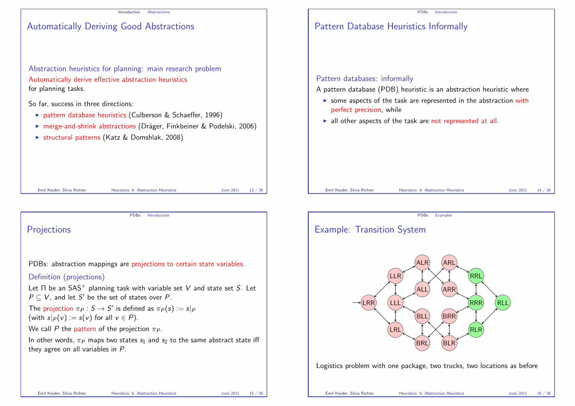
Introduction Abstractions
Automatically Deriving Good Abstractions
Abstraction heuristics for planning: main research problemAutomatically derive effective abstraction heuristicsfor planning tasks.
So far, success in three directions:
� pattern database heuristics (Culberson & Schaeffer, 1996)
� merge-and-shrink abstractions (Drager, Finkbeiner & Podelski, 2006)
� structural patterns (Katz & Domshlak, 2008)
Emil Keyder, Silvia Richter Heuristics: 6. Abstraction Heuristics June 2011 13 / 36
PDBs Introduction
Pattern Database Heuristics Informally
Pattern databases: informallyA pattern database (PDB) heuristic is an abstraction heuristic where
� some aspects of the task are represented in the abstraction withperfect precision, while
� all other aspects of the task are not represented at all.
Emil Keyder, Silvia Richter Heuristics: 6. Abstraction Heuristics June 2011 14 / 36
PDBs Introduction
Projections
PDBs: abstraction mappings are projections to certain state variables.
Definition (projections)
Let Π be an SAS+ planning task with variable set V and state set S . LetP ⊆ V , and let S � be the set of states over P .
The projection πP : S → S � is defined as πP(s) := s|P(with s|P(v) := s(v) for all v ∈ P).
We call P the pattern of the projection πP .
In other words, πP maps two states s1 and s2 to the same abstract state iffthey agree on all variables in P .
Emil Keyder, Silvia Richter Heuristics: 6. Abstraction Heuristics June 2011 15 / 36
PDBs Examples
Example: Transition System
LRR LLL
LLR
LRL
ALR
ALL
BLL
BRL
ARL
ARR
BRR
BLR
RRR
RRL
RLR
RLL
Logistics problem with one package, two trucks, two locations as before
Emil Keyder, Silvia Richter Heuristics: 6. Abstraction Heuristics June 2011 16 / 36
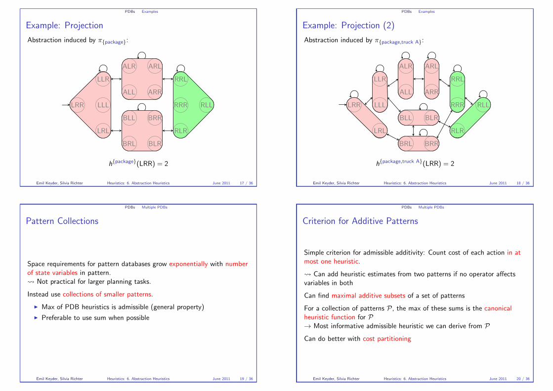
PDBs Examples
Example: Projection
Abstraction induced by π{package}:
LRR LLL
LLR
LRL
LRR
LLR
LRL
LLL
ALR ARL
ALL ARR
ALR ARL
ARRALL
BLL
BRL
BRR
BLR
BLL BRR
BLRBRL
RRR
RRL
RLR
RLLRLL
RRL
RLR
RRR
h{package}(LRR) = 2
Emil Keyder, Silvia Richter Heuristics: 6. Abstraction Heuristics June 2011 17 / 36
PDBs Examples
Example: Projection (2)
Abstraction induced by π{package,truck A}:
LRR
LRL
LRR
LRL
LLL
LLRLLR
LLL
ALR
ALL
ALR
ALL
ARL
ARR
ARL
ARR
BRR
BLL BLR
BRL
BLL BLR
BRL BRR
RRR
RRLRRL
RRR
RLR
RLLRLL
RLR
h{package,truck A}(LRR) = 2
Emil Keyder, Silvia Richter Heuristics: 6. Abstraction Heuristics June 2011 18 / 36
PDBs Multiple PDBs
Pattern Collections
Space requirements for pattern databases grow exponentially with numberof state variables in pattern.� Not practical for larger planning tasks.
Instead use collections of smaller patterns.
� Max of PDB heuristics is admissible (general property)
� Preferable to use sum when possible
Emil Keyder, Silvia Richter Heuristics: 6. Abstraction Heuristics June 2011 19 / 36
PDBs Multiple PDBs
Criterion for Additive Patterns
Simple criterion for admissible additivity: Count cost of each action in atmost one heuristic.
� Can add heuristic estimates from two patterns if no operator affectsvariables in both
Can find maximal additive subsets of a set of patterns
For a collection of patterns P, the max of these sums is the canonicalheuristic function for P→ Most informative admissible heuristic we can derive from P
Can do better with cost partitioning
Emil Keyder, Silvia Richter Heuristics: 6. Abstraction Heuristics June 2011 20 / 36
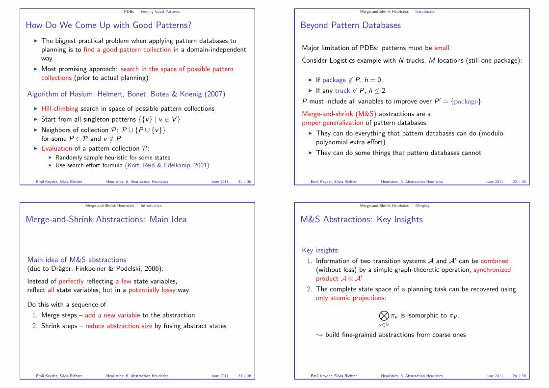
PDBs Finding Good Patterns
How Do We Come Up with Good Patterns?
� The biggest practical problem when applying pattern databases toplanning is to find a good pattern collection in a domain-independentway.
� Most promising approach: search in the space of possible patterncollections (prior to actual planning)
Algorithm of Haslum, Helmert, Bonet, Botea & Koenig (2007)
� Hill-climbing search in space of possible pattern collections
� Start from all singleton patterns {{v} | v ∈ V }� Neighbors of collection P: P ∪ {P ∪ {v}}
for some P ∈ P and v /∈ P
� Evaluation of a pattern collection P:� Randomly sample heuristic for some states� Use search effort formula (Korf, Reid & Edelkamp, 2001)
Emil Keyder, Silvia Richter Heuristics: 6. Abstraction Heuristics June 2011 21 / 36
Merge-and-Shrink Heuristics Introduction
Beyond Pattern Databases
Major limitation of PDBs: patterns must be small
Consider Logistics example with N trucks, M locations (still one package):
� If package �∈ P , h = 0
� If any truck �∈ P , h ≤ 2
P must include all variables to improve over P � = {package}
Merge-and-shrink (M&S) abstractions are aproper generalization of pattern databases.
� They can do everything that pattern databases can do (modulopolynomial extra effort)
� They can do some things that pattern databases cannot
Emil Keyder, Silvia Richter Heuristics: 6. Abstraction Heuristics June 2011 22 / 36
Merge-and-Shrink Heuristics Introduction
Merge-and-Shrink Abstractions: Main Idea
Main idea of M&S abstractions(due to Drager, Finkbeiner & Podelski, 2006):
Instead of perfectly reflecting a few state variables,reflect all state variables, but in a potentially lossy way.
Do this with a sequence of
1. Merge steps – add a new variable to the abstraction
2. Shrink steps – reduce abstraction size by fusing abstract states
Emil Keyder, Silvia Richter Heuristics: 6. Abstraction Heuristics June 2011 23 / 36
Merge-and-Shrink Heuristics Merging
M&S Abstractions: Key Insights
Key insights:
1. Information of two transition systems A and A� can be combined(without loss) by a simple graph-theoretic operation, synchronizedproduct A⊗A�
2. The complete state space of a planning task can be recovered usingonly atomic projections:
�
v∈Vπv is isomorphic to πV .
� build fine-grained abstractions from coarse ones
Emil Keyder, Silvia Richter Heuristics: 6. Abstraction Heuristics June 2011 24 / 36
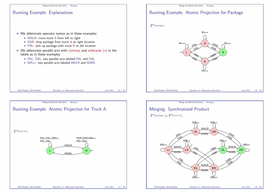
Merge-and-Shrink Heuristics Merging
Running Example: Explanations
� We abbreviate operator names as in these examples:� MALR: move truck A from left to right� DAR: drop package from truck A at right location� PBL: pick up package with truck B at left location
� We abbreviate parallel arcs with commas and wildcards (�) in thelabels as in these examples:
� PAL, DAL: two parallel arcs labeled PAL and DAL� MA��: two parallel arcs labeled MALR and MARL
Emil Keyder, Silvia Richter Heuristics: 6. Abstraction Heuristics June 2011 25 / 36
Merge-and-Shrink Heuristics Merging
Running Example: Atomic Projection for Package
T π{package} :
L
A
B
R
M���PA
L
DAL
M���
DARPAR
M���
PBR
DBR
M���
DBL
PBL
Emil Keyder, Silvia Richter Heuristics: 6. Abstraction Heuristics June 2011 26 / 36
Merge-and-Shrink Heuristics Merging
Running Example: Atomic Projection for Truck A
T π{truck A} :
L R
PAL,DAL,MB��,PB�,DB�
MALR
MARL
PAR,DAR,MB��,PB�,DB�
Emil Keyder, Silvia Richter Heuristics: 6. Abstraction Heuristics June 2011 27 / 36
Merge-and-Shrink Heuristics Merging
Merging: Synchronized Product
T π{package} ⊗ T π{truck A} :
LL LR
AL AR
BL BR
RL RRMALR
MARL
MALR
MARL
MALR
MARL
MALR
MARL
PAL
DAL
DAR
PAR
PBRD
BR
DBL
PBL
PBL
DBL
DBR
PBR
MB�� MB��
MB�� MB��
MB�� MB��
MB�� MB��
Emil Keyder, Silvia Richter Heuristics: 6. Abstraction Heuristics June 2011 28 / 36
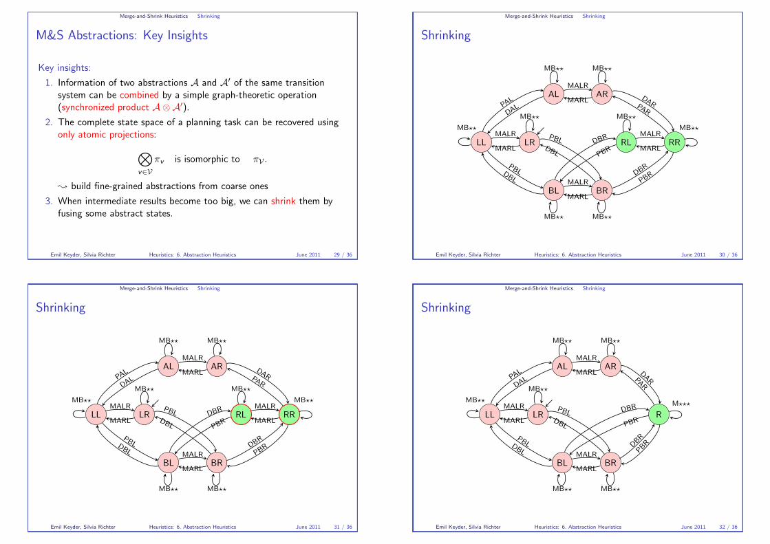
Merge-and-Shrink Heuristics Shrinking
M&S Abstractions: Key Insights
Key insights:
1. Information of two abstractions A and A� of the same transitionsystem can be combined by a simple graph-theoretic operation(synchronized product A⊗A�).
2. The complete state space of a planning task can be recovered usingonly atomic projections:
�
v∈Vπv is isomorphic to πV .
� build fine-grained abstractions from coarse ones
3. When intermediate results become too big, we can shrink them byfusing some abstract states.
Emil Keyder, Silvia Richter Heuristics: 6. Abstraction Heuristics June 2011 29 / 36
Merge-and-Shrink Heuristics Shrinking
Shrinking
LL LR
AL AR
BL BR
RL RRMALR
MARL
MALR
MARL
MALR
MARL
MALR
MARL
PAL
DAL
DARPA
R
PBRD
BR
DBL
PBL
PBL
DBL
DBR
PBR
MB�� MB��
MB�� MB��
MB�� MB��
MB�� MB��
Emil Keyder, Silvia Richter Heuristics: 6. Abstraction Heuristics June 2011 30 / 36
Merge-and-Shrink Heuristics Shrinking
Shrinking
LL LR
AL AR
BL BR
RL RRMALR
MARL
MALR
MARL
MALR
MARL
MALR
MARL
PAL
DAL
DARPA
R
PBRD
BR
DBL
PBL
PBL
DBL
DBR
PBR
MB�� MB��
MB�� MB��
MB�� MB��
MB�� MB��
Emil Keyder, Silvia Richter Heuristics: 6. Abstraction Heuristics June 2011 31 / 36
Merge-and-Shrink Heuristics Shrinking
Shrinking
LL LR
AL AR
BL BR
RMALR
MARL
MALR
MARL
MALR
MARL
PAL
DAL
DARP
AR
PBRD
BR
DBL
PBL
PBL
DBL
DBR
PBR
MB��
MB�� MB��
MB��
MB��
M���
MB��
Emil Keyder, Silvia Richter Heuristics: 6. Abstraction Heuristics June 2011 32 / 36
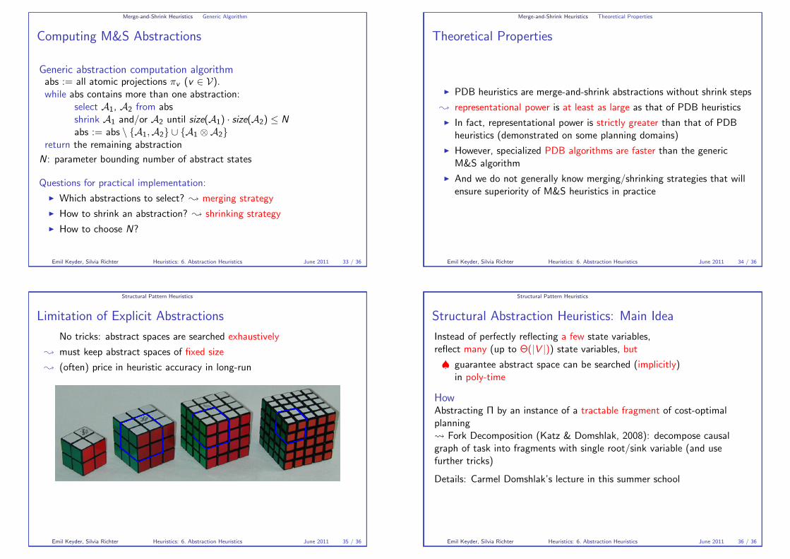
Merge-and-Shrink Heuristics Generic Algorithm
Computing M&S Abstractions
Generic abstraction computation algorithmabs := all atomic projections πv (v ∈ V).while abs contains more than one abstraction:
select A1, A2 from absshrink A1 and/or A2 until size(A1) · size(A2) ≤ N
abs := abs \ {A1,A2} ∪ {A1 ⊗A2}return the remaining abstraction
N: parameter bounding number of abstract states
Questions for practical implementation:
� Which abstractions to select? � merging strategy
� How to shrink an abstraction? � shrinking strategy
� How to choose N?
Emil Keyder, Silvia Richter Heuristics: 6. Abstraction Heuristics June 2011 33 / 36
Merge-and-Shrink Heuristics Theoretical Properties
Theoretical Properties
� PDB heuristics are merge-and-shrink abstractions without shrink steps
� representational power is at least as large as that of PDB heuristics
� In fact, representational power is strictly greater than that of PDBheuristics (demonstrated on some planning domains)
� However, specialized PDB algorithms are faster than the genericM&S algorithm
� And we do not generally know merging/shrinking strategies that willensure superiority of M&S heuristics in practice
Emil Keyder, Silvia Richter Heuristics: 6. Abstraction Heuristics June 2011 34 / 36
Structural Pattern Heuristics
Limitation of Explicit Abstractions
No tricks: abstract spaces are searched exhaustively
� must keep abstract spaces of fixed size
� (often) price in heuristic accuracy in long-run
Emil Keyder, Silvia Richter Heuristics: 6. Abstraction Heuristics June 2011 35 / 36
Structural Pattern Heuristics
Structural Abstraction Heuristics: Main Idea
Instead of perfectly reflecting a few state variables,reflect many (up to Θ(|V |)) state variables, but
♠ guarantee abstract space can be searched (implicitly)in poly-time
HowAbstracting Π by an instance of a tractable fragment of cost-optimalplanning� Fork Decomposition (Katz & Domshlak, 2008): decompose causalgraph of task into fragments with single root/sink variable (and usefurther tricks)
Details: Carmel Domshlak’s lecture in this summer school
Emil Keyder, Silvia Richter Heuristics: 6. Abstraction Heuristics June 2011 36 / 36

Heuristics for Domain-Independent Planning7. Final Comments
Emil Keyder Silvia Richter
Based partially on slides by Carmel Domshlak and Malte Helmert
ICAPS 2011 Summer School on Automated Planning and Scheduling
June 2011
Emil Keyder, Silvia Richter Heuristics: 7. Final Comments June 2011 1 / 7
Satisficing PlanningBeyond Heuristics
Optimal Planning
Emil Keyder, Silvia Richter Heuristics: 7. Final Comments June 2011 2 / 7
Connecting the Pieces
� We have seen a number of heuristics in this tutorial,for satisficing and optimal planning
� Now the big question is:
Which ones work best?And what’s there beyond heuristics to improve planning-by-search?
Emil Keyder, Silvia Richter Heuristics: 7. Final Comments June 2011 3 / 7
Satisficing Planning
Satisficing vs. Optimal Planning
Satisficing and optimal planning are much more different from each otherthan it appears at a superficial glance.
� Optimal planning entails proving that there is no better solution
� As a consequence, A∗-based planning requires exponential effort inmost domains even with almost perfect heuristics (Helmert & Roger,2008).
� Not so for satisficing planning, where just finding a solution is enough
Emil Keyder, Silvia Richter Heuristics: 7. Final Comments June 2011 4 / 7
Satisficing Planning Beyond Heuristics
Satisficing Planning: Beyond Heuristics
� Because satisficing planners do not need to prove optimality, they canuse drastic search control strategies
� These often make a larger difference in performancethan the choice of heuristic function (Richter & Helmert, 2009)
Examples:
� helpful actions (FF: Hoffmann & Nebel, 2001)
� relaxed plan macros (YAHSP: Vidal, 2004)
� preferred operators (Fast Downward, LAMA: Helmert, 2006)
� alternating multi-queue search (Fast Downward, LAMA: Helmert &Roger, 2010)
Emil Keyder, Silvia Richter Heuristics: 7. Final Comments June 2011 5 / 7
Satisficing Planning Beyond Heuristics
Satisficing Planning: Conclusion
� Satisficing heuristics with good coverage (given limited time) are e. g.the FF heuristic and the context-enhanced additive heuristic,whereas the additive heuristic and inadmissible landmark-counting (bythemselves) are less strong
� Picture less clear when measuring quality in addition to coverage (�question of trade-off),in particular when planning with action costs
E. g. cost-insensitive variant of FF heuristic dominates cost-sensitiveone in terms of the IPC 2008 criterion (Richter & Westphal, 2010)
Emil Keyder, Silvia Richter Heuristics: 7. Final Comments June 2011 6 / 7
Optimal Planning
Optimal Planning: Conclusion
� Landmark heuristics like hLA and hLM-cut shown to outperformadditive hmax and abstraction heuristics like PDBs and M&S (undertypical competition conditions)
� Theoretical results show M&S has the power to be more informativethan PDBs and landmark heuristics, while additive hmax ∼ landmarks(Helmert & Domshlak, 2009)
� But worth keeping in mind that higher accuracy does not necessarilypay off when time is limited
Emil Keyder, Silvia Richter Heuristics: 7. Final Comments June 2011 7 / 7
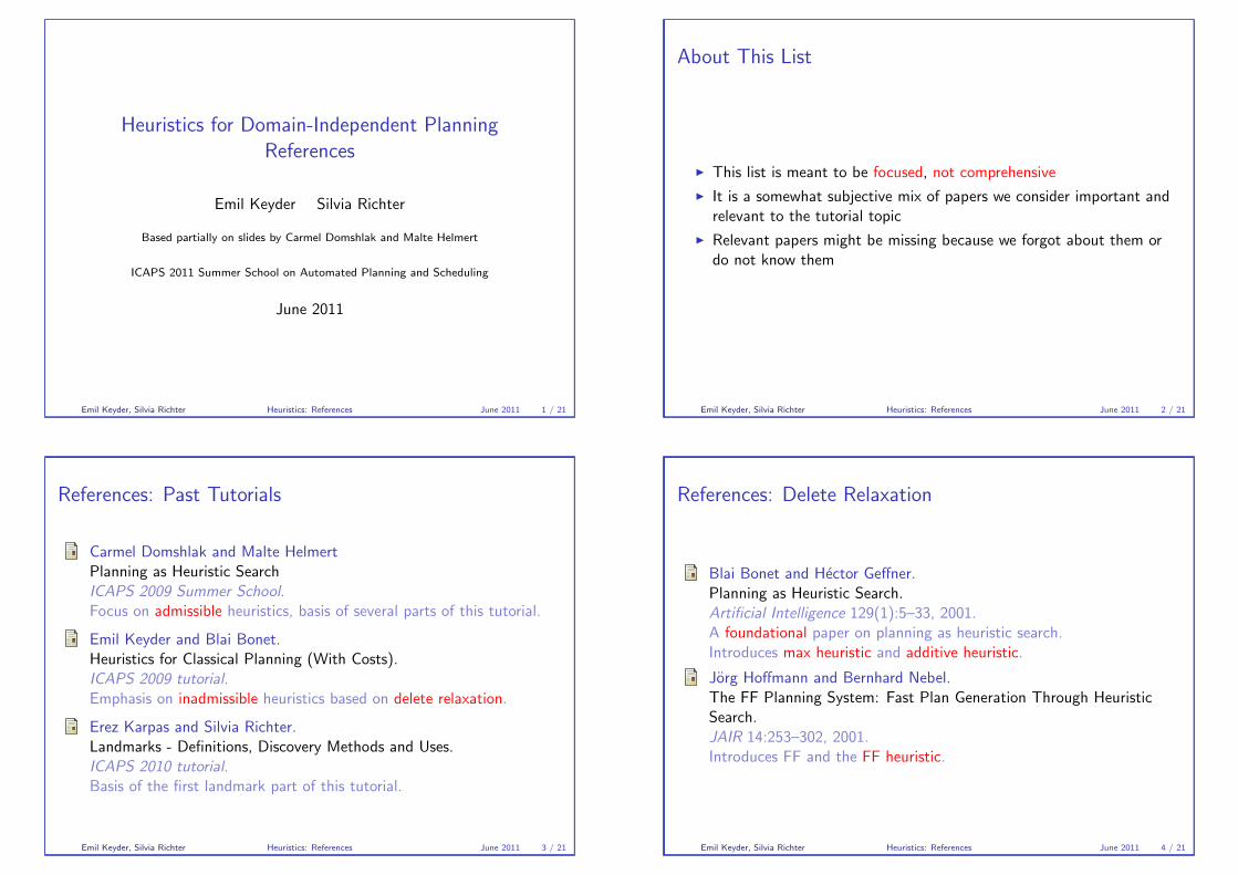
Heuristics for Domain-Independent Planning
References
Emil Keyder Silvia Richter
Based partially on slides by Carmel Domshlak and Malte Helmert
ICAPS 2011 Summer School on Automated Planning and Scheduling
June 2011
Emil Keyder, Silvia Richter Heuristics: References June 2011 1 / 21
About This List
� This list is meant to be focused, not comprehensive
� It is a somewhat subjective mix of papers we consider important andrelevant to the tutorial topic
� Relevant papers might be missing because we forgot about them ordo not know them
Emil Keyder, Silvia Richter Heuristics: References June 2011 2 / 21
References: Past Tutorials
Carmel Domshlak and Malte HelmertPlanning as Heuristic SearchICAPS 2009 Summer School.Focus on admissible heuristics, basis of several parts of this tutorial.
Emil Keyder and Blai Bonet.Heuristics for Classical Planning (With Costs).ICAPS 2009 tutorial.Emphasis on inadmissible heuristics based on delete relaxation.
Erez Karpas and Silvia Richter.Landmarks - Definitions, Discovery Methods and Uses.ICAPS 2010 tutorial.Basis of the first landmark part of this tutorial.
Emil Keyder, Silvia Richter Heuristics: References June 2011 3 / 21
References: Delete Relaxation
Blai Bonet and Hector Geffner.Planning as Heuristic Search.Artificial Intelligence 129(1):5–33, 2001.A foundational paper on planning as heuristic search.Introduces max heuristic and additive heuristic.
Jorg Hoffmann and Bernhard Nebel.The FF Planning System: Fast Plan Generation Through HeuristicSearch.JAIR 14:253–302, 2001.Introduces FF and the FF heuristic.
Emil Keyder, Silvia Richter Heuristics: References June 2011 4 / 21

References: Delete Relaxation (ctd.)
Emil Keyder and Hector Geffner.Heuristics for Planning with Action Costs Revisited.Proc. ECAI 2008, pp. 588–592, 2008.Introduces cost-sensitive FF/additive and set-additive heuristics.
Emil Keyder and Hector Geffner.Trees of Shortest Paths vs. Steiner Trees: Understanding andImproving Delete Relaxation Heuristics.Proc. IJCAI 2009, pp. 1734–1739, 2009.Introduces Steiner tree heuristic, improving the accuracy ofinadmissible delete relaxation heuristics.
Emil Keyder, Silvia Richter Heuristics: References June 2011 5 / 21
References: Delete Relaxation (ctd.)
Yaxin Liu, Sven Koenig and David Furcy.Speeding Up the Calculation of Heuristics for Heuristic Search-BasedPlanning.Proc. AAAI 2002, pp. 484–491, 2002.Discussion of different methods for computing delete relaxationheuristics.
Emil Keyder, Silvia Richter Heuristics: References June 2011 6 / 21
References: Landmarks
Jorg Hoffmann, Julie Porteous and Laura Sebastia.Ordered Landmarks in Planning.JAIR 22:215–278, 2004.Journal version of the first landmarks paper.
Silvia Richter and Matthias Westphal.The LAMA Planner: Guiding Cost-Based Anytime Planning withLandmarks.JAIR 2010, pp. 127–177, 2010.Describes the landmark-counting heuristic and compares cost-sensitivevs. cost-insensitive variants of the FF heuristic.
Erez Karpas and Carmel Domshlak.Cost-Optimal Planning with Landmarks.Proc. IJCAI 2009, pp. 1728–1733, 2009.Introduces admissible landmark heuristics based on cost partitioning.
Emil Keyder, Silvia Richter Heuristics: References June 2011 7 / 21
References: Landmarks (ctd.)
Emil Keyder, Silvia Richter, and Malte Helmert.Sound and Complete Landmarks for AND/OR Graphs.Proc. ECAI 2010, pp. 335–340, 2010.Complete landmark finding and landmarks beyond the deleterelaxation.
Malte Helmert and Carmel Domshlak.Landmarks, Critical Paths and Abstractions: What’s the DifferenceAnyway?Proc. ICAPS 2009, pp. 162–169, 2009Introduces the landmark cut heuristic.
Blai Bonet and Malte Helmert.Strengthening Landmark Heuristics via Hitting Sets.Proc. ECAI 2010, pp. 329–334, 2010.Improving the accuracy of the landmark cut heuristic.
Emil Keyder, Silvia Richter Heuristics: References June 2011 8 / 21
References: Critical Path
Patrik Haslum and Hector GeffnerAdmissible Heuristics for Optimal Planning.Proc. AIPS 2000, pp. 140–149, 2000.Introduces critical path heuristics.
Patrik Haslumhm(P) = h1(Pm): Alternative Characterisations of the GeneralisationFrom hmax to hm.Proc. ICAPS 2009, pp. 354–357, 2009.Introduces Pm compilation.
Emil Keyder, Silvia Richter Heuristics: References June 2011 9 / 21
References: Pattern Databases
Stefan Edelkamp.Planning with Pattern Databases.Proc. ECP 2001, pp. 13–24, 2001.First paper on planning with pattern databases.
Stefan Edelkamp.Symbolic Pattern Databases in Heuristic Search Planning.Proc. AIPS 2002, pp. 274–283, 2002.Uses BDDs to store pattern databases more compactly.
Emil Keyder, Silvia Richter Heuristics: References June 2011 10 / 21
References: Pattern Databases (ctd.)
Patrik Haslum, Blai Bonet and Hector Geffner.New Admissible Heuristics for Domain-Independent Planning.Proc. AAAI 2005, pp. 1163–1168, 2005.Introduces constrained PDBs.First pattern selection methods based on heuristic quality.
Stefan Edelkamp.Automated Creation of Pattern Database Search Heuristics.Proc. MoChArt 2006, pp. 121–135, 2007.First search-based pattern selection method.
Emil Keyder, Silvia Richter Heuristics: References June 2011 11 / 21
References: Pattern Databases (ctd.)
Patrik Haslum, Malte Helmert, Adi Botea, Blai Bonet and SvenKoenig.Domain-Independent Construction of Pattern Database Heuristics forCost-Optimal Planning.Proc. AAAI 2007, pp. 1007–1012, 2007.Introduces canonical heuristic for pattern collections.Search-based pattern selection based on Korf, Reid & Edelkamp’stheory.
Marcel Ball and Robert C. Holte.The Compression Power of Symbolic Pattern Databases.Proc. ICAPS 2008, pp. 2–11, 2008.Detailed empirical analysis showing benefits of symbolic BDDs overexplicit-state BDDs.
Emil Keyder, Silvia Richter Heuristics: References June 2011 12 / 21

References: Merge & Shrink
Klaus Drager, Bernd Finkbeiner and Andreas Podelski.Directed Model Checking with Distance-Preserving Abstractions.Proc. SPIN 2006, pp. 19–34, 2006.Introduces merge-and-shrink abstractions(for model-checking).
Malte Helmert, Patrik Haslum and Jorg Hoffmann.Flexible Abstraction Heuristics for Optimal Sequential Planning.Proc. ICAPS 2007, pp. 176–183, 2007.Introduces merge-and-shrink abstractions for planning.
Emil Keyder, Silvia Richter Heuristics: References June 2011 13 / 21
References: Merge & Shrink (ctd.)
Raz Nissim, Jorg Hoffmann, and Malte Helmert.Computing Perfect Heuristics in Polynomial Time: On Bisimulationand Merge-and-Shrink Abstraction in Optimal Planning.Proc. IJCAI 2011, 2011.New stragies for computing merge-and-shrink abstractions.
Emil Keyder, Silvia Richter Heuristics: References June 2011 14 / 21
References: Structural Patterns
Michael Katz and Carmel Domshlak.Structural Patterns Heuristics via Fork Decomposition.Proc. ICAPS 2008, pp. 182–189, 2008.Introduces structural-pattern abstractions, and studiesfork-decomposition structural patterns.
Michael Katz and Carmel Domshlak.Structural-Pattern Databases.Proc. ICAPS 2009, pp. 186–193, 2009.Introduces structural-pattern databases, making the idea offork-decomposition practical.
Carmel Domshlak, Michael Katz and Sagi LeflerWhen Abstractions Met LandmarksProc. ICAPS 2010, pp. 50–56, 2010.Improving abstraction heuristics with landmark information.
Emil Keyder, Silvia Richter Heuristics: References June 2011 15 / 21
References: Causal Graph Heuristics
Malte Helmert.A Planning Heuristic Based on Causal Graph Analysis.Proc. ICAPS 2004, pp. 161–170, 2004.Introduces causal graph heuristic.
Malte Helmert and Hector Geffner.Unifying the Causal Graph and Additive Heuristics.Proc. ICAPS 2008, pp. 140–147, 2008.Introduces context-enhanced additive heuristic, combining the featuresof the causal graph and additive heuristics.
Dunbo Cai, Jorg Hoffmann and Malte HelmertEnhancing the Context-Enhanced Additive Heuristic with PrecedenceConstraintsProc. ICAPS 2009, 2009.Explores precedence relations in the context enhanced additiveheuristic.
Emil Keyder, Silvia Richter Heuristics: References June 2011 16 / 21
References: Heuristic Performance
Malte Helmert and Gabriele Roger.How Good is Almost Perfect?Proc. AAAI 2008, pp. 944–949, 2008.Shows that optimal planning is hard even with almost perfectheuristics differing from h∗ by an additive constant.
Malte Helmert and Robert Mattmuller.Accuracy of Admissible Heuristic Functions in Selected PlanningDomains.Proc. AAAI 2008, pp. 938–943, 2008.Introduces asymptotic accuracy of admissible heuristics.
Emil Keyder, Silvia Richter Heuristics: References June 2011 17 / 21
References: Search Enhancements
Jorg Hoffmann and Bernhard Nebel.The FF Planning System: Fast Plan Generation Through HeuristicSearch.JAIR 14:253–302, 2001.Introduces relaxed plans and helpful action pruning.
Vincent Vidal.A Lookahead Strategy for Heuristic Search Planning.In Proc. ICAPS 2004, pp. 150–159, 2004.Takes helpful actions further with relaxed plan macros.
Malte Helmert.The Fast Downward Planning System.JAIR 26:191–246, 2006.Introduces preferred operators, alternating multi-queue search, anddelayed evaluation for systematic best-first search algorithms.
Emil Keyder, Silvia Richter Heuristics: References June 2011 18 / 21
References: Search Enhancements (ctd.)
Silvia Richter and Malte Helmert.Preferred Operators and Deferred Evaluation in Satisficing Planning.Proc. ICAPS 2009, pp. 273–280, 2009.Empirical evaluation of various strategies for preferred operators.
Gabriele Roger and Malte Helmert.The More, the Merrier: Combining Heuristic Estimators for SatisficingPlanning.Proc. ICAPS 2010, pp. 246–249, 2010.Empirical evaluation of various strategies for combining severalheuristics.
Emil Keyder, Silvia Richter Heuristics: References June 2011 19 / 21
References: Heuristic Analysis & Comparison (ctd.)
Michael Katz and Carmel Domshlak.Optimal Additive Composition of Abstraction-based AdmissibleHeuristics.Proc. ICAPS 2008, pp. 174–181, 2008.Introduces action cost partitioning, and proves tractability of optimalpartitions for (numerous types of) abstractions.
Malte Helmert and Carmel Domshlak.Landmarks, Critical Paths and Abstractions: What’s the DifferenceAnyway?Proc. ICAPS 2009, pp. 162–169, 2009.Uses cost partitioning to prove formal compilability results betweenvarious classes of heuristics.
Emil Keyder, Silvia Richter Heuristics: References June 2011 20 / 21

References: Heuristic Analysis & Comparison
Jorg Hoffmann.Where Ignoring Delete Lists Works, Part II: Causal GraphsProc. ICAPS 2011, 2011.Automated analysis of delete-relaxation heuristics on differentdomains.
Emil Keyder, Silvia Richter Heuristics: References June 2011 21 / 21