Heterogeneous technology and panel data: The case of the agricultural production function

Yair Mundlaka, Rita Butzerb and Donald F. Larsonc

________________________________________________________________________

Abstract

The paper presents empirical analysis of a panel of countries aimed at estimating

agricultural production using a measure of capital in agriculture absent from most studies.

We employ a heterogeneous technology framework where implemented technology is

chosen jointly with inputs to interpret information obtained in the empirical analysis of

panel data. We discuss the scope for replacing country and time effects by observed

variables and the limitations of instrumental variables. The empirical results differ from

those reported in the literature for cross-country studies, largely in augmenting the

elasticities of capital and land and reducing those of fertilizers and labor.

_________________________________________________________________________

JEL classifications: C230, D240, Q110, O130

Keywords: Agriculture, development, economic growth, panel data, productivity

Acknowledgment We thank Yacov Tsur for helpful comments. This study was funded by the Bank’s Research Support Budget under the research project, “The Contributions of Governance to Growth in Agriculture" (RP0 94759).

a Corresponding author. E-mail address: mundlak@agri.huji.ac.il. Professor Emeritus, Hebrew University of Jerusalem. b Ph.D.Candidate, Economics, The University of Chicago. c Senior Research Economist, World Bank.

Heterogeneous technology and panel data:

The case of the agricultural production function

Introduction

The focus of empirical analysis of agricultural production functions, similar to that

of production functions in general, has changed over the years.1 Following the work of

Cobb and Douglas (1928), research centered on questions about the efficiency of the factor

markets. Research interest subsequently shifted to issues related to changes in factor

demand, leading to interest in the elasticity of substitution, to factor augmentation, to a

search for the proper algebraic form, to issues related to aggregation, and more recently to

issues related to the variability in income and in productivity growth. The statistical

aspects of the analysis were affected by the recognition of the endogeneity of the inputs,

raised by Marschak and Andrews (1944), and by the methods of accommodating this

complication in the estimation. This led to the use of panel data, to the dual approach to the

estimation, and to the use of instrumental variables.

A common assumption in much of the work was that of a homogeneous

technology, implying that a common production function generated observations used in

the analysis. In reality, firms face the practical problem of choosing which technology to

employ jointly with inputs so that technology is heterogeneous in that there is more than

one function associated with the data. In this paper we examine the consequences of this

extension in estimating an aggregate agricultural production function using panel data,

where the underlying functions are all of the Cobb-Douglas form. We model the

technology choice as conditional on predetermined variables referred to as state variables.

This approach provides a different view of the empirical results of most of the

aforementioned subjects. The root of the difference is the recognition that the observations

in the sample represent moves between functions as well as movements along a given

function. The empirical formulation allows for the dependence of parameters of the

1 For the development of the work on agricultural production functions, see Mundlak (2001).

2

function, just as the inputs, on the state variables, and in this sense the observed, or

implemented, technology is endogenous.

The paper is oriented toward the understanding of the role of inputs and technology

in agriculture. Although the subject has a long history, it is still relevant, and is related,

among other things, to the interest in structural changes that take place in the process of

economic development. This topic of inquiry has real world implications because most of

the poor households in developing countries live in rural areas and depend on agriculture

for their livelihood.2 An increase in agricultural productivity directly contributes to the

welfare of the rural area. Changes in factor demand due to changes in technology affect the

intersectoral flow of resources, primarily labor and capital, which constitutes the essence of

the structural changes in the process of development. Understanding this process has

policy implications concerning what is worth doing and what is worth avoiding.

The analysis is related to the macroeconomic literature on the determinants of

economic growth and productivity for overall economies. The models used vary in the

parsimony of the parametric specification and in the choice of what parameters are to be

estimated and those to be imposed. The heterogeneity of approaches reflects the inability to

obtain empirically reliable and robust results that follow from basic economic reasoning.

This feeds the search for better specifications and for the appropriate ways of handling the

data. Most growth studies include a set of core Solow-Swan variables related to human

capital investment, physical capital investment, initial income conditions and either

population or labor growth.3 Studies of differences in productivity levels use similar

variables. There is less of a consensus on the broader set of state variables, though a

growing interest has arisen in the role of certain state variables such as culture, geography,

institutions, and market integration.4 Defined very broadly, institutions include the

humanly devised rules that shape economic incentives and that are particularly related to

the protection of property, the enforcement of contracts, and the dissemination of

information (North 1990; Acemoglu, Johnson, and Robinson 2005). There is no unity in

2 According to the World Bank (2007), this includes 2.1 billion people living on less than $2 a day. 3 See for instance the review by Durlauf, Johnson, and Temple (2005) and Durlauf and Quah (1999). 4 See, for example, Sachs and Warner (1997), Hall and Jones (1999), Rodrik, Subramanian, and Trebbi (2004), and Presbitero (2006).

3

how the state variables are to be used in the analysis. In some models they are assumed to

be the sole causes of accumulation and productivity changes (Hall and Jones 1999), while

in others they are added to inputs in the estimation of the production function. They are

also used as instrumental variables to deal with endogeneity of inputs, institutions, and

measurement errors.

Finding a set of variables that adequately describes prevailing economic incentives

is challenging for several reasons. First, while the objective of most research is to get at the

long-run determinants of economic growth, much of the variation in economic activity,

and thus in the data, is associated with short-term fluctuations, which may be linked to

quasi-fixed constraints or gaps caused by misplaced expectations. Second, economic

growth theory is open-ended, and the set of potential determinants of economic incentives

is large relative to the panel datasets available for studying macroeconomic growth.5

As a practical matter, many empirical models deal with the prevalence of short-

term variability in the data by averaging across periods, and thereby affect the empirical

results.6 Even so, some authors argue that this type of transformation is not arbitrary but

rather necessary to eliminate nuisance variations and potential biases.7 As we show, the

short-term variations are essential for identifying the production function, and thereby to

obtain the appropriate weights for calculating total factor (TF) and total factor productivity

(TFP). On the other hand, weights based on country averages provide distorted estimates

of productivity.8

In terms of end results, part of the debate involves the importance of total factor

productivity relative to accumulations of human and physical capital in determining

patterns of growth. For example, Mankiw, Romer, and Weil (1992) and Henderson and

Russell (2005) find that accumulations largely account for growth, while Klenow and

Rodriguez-Clare (1997) and Easterly and Levine (2001) place greater emphasis on

productivity growth. 5 In their review of applied macroeconomic growth studies, Durlauf, Johnson, and Temple (2005) compile a set of 145 variables that have been used as growth determinants. 6 For a review of applied techniques based on growth rates, see Durlauf, Johnson, and Temple (2005). 7 See, for example, Pritchett (2000). 8 See, for example, Sala-i-Martin, Doppelhofer, and Miller (2004).

4

Similarly, a variety of conclusions are reached concerning the core set of state

variables. Hall and Jones (1999) emphasize the role of social capital and Rodrik,

Subramanian, and Trebbi (2004) assert the dominance of institutions over other

determinants. In other papers, trade, monetary policy, and cultural factors related to

religion, language, and colonial heritage are viewed as key determinants.9 But in their

review of the recent literature, Durlauf, Johnson, and Temple (2005, p. 558) conclude that

“(e)ven when the study of growth is viewed in terms of a collective endeavor, the various

papers cannot easily be distilled into a consensus that would meet standards of evidence

routinely applied in other fields of economics.”

In terms of this literature, we deal with a sectoral production function, representing

a lower level of aggregation, but many of the issues still remain here as well. Agricultural

output has grown as a result of changes in technology and in resource allocation where the

role of labor declined and that of capital increased. Regarding the decomposition of the

output growth to TF and TFP, we rely on the empirical estimates of the production

function parameters, and as such the outcome depends on the quality of the estimates.

When the parameters of the production function depend on the state variables, the relative

contribution of the TF and the TFP is also endogenous; hence TFP can not be considered

to be the trigger of growth but rather is a result of it. The dependence of the parameters on

the state variables accounts for the wide spread in the empirical results reported in the

literature.10

The inputs used in the analysis are land, capital, fertilizer, and labor. The capital

variables, constructed for this analysis, revise and update an earlier series that was used in

Mundlak, Larson, and Butzer (1999). The state variables consist of variables representing

technology, institutions, incentives, and physical environment. A substantial portion of the

empirical section of the paper is devoted to finding a robust set of variables that adequately

accounts for agricultural output differences not explained by factors of production.

9 For example, Frankel and Romer (1999) and Sachs and Warner (1997) discuss the role of trade. Examples related to exchange rates include Dollar (1992) and Barro and Lee (1994). Barro and McCleary (2003), among others, write about the role of religion. 10 Mundlak, Larson, and Butzer (1999) summarize the empirical agricultural production functions based on cross-country data that had appeared prior to the writing of the paper. More studies have appeared since, but they only confirm the existence of diversity of the results.

5

I. The model

The underlying premise is that producers at any time face more than one technique

of production, and their economic problem is to choose the techniques to be employed

together with the choice of inputs and outputs. The outline of the approach follows

Mundlak (1988, 1993). Let X be the vector of inputs and Fj(X) be the production function

associated with the jth technique, where Fj is concave and twice differentiable, and define

the available technology, T, as the collection of all possible techniques, T = {Fj(X);

j=1,...,J}. Firms choose the implemented techniques subject to their constraints and the

environment. We distinguish between constrained (K) and unconstrained (V) inputs,

X=(V,K), and assume for simplicity, without a loss of generality, that the constrained

inputs have no alternative cost. Prices for inputs (W) and output (P) are given by the

markets. The optimization problem calls for a choice of the level of inputs to be assigned

to technique j so as to maximize profits. To simplify the presentation, we deal with a

comparative statics framework and therefore omit a time index for the variables. The

extension to the intertemporal version is conceptually straightforward.

Ignoring the analytic details, we turn to characterize the solution and its

implication. Let s=(K,P,W,T) be the vector of state variables of this problem and write the

solution as: Vj*(s), Kj*(s), to emphasize the dependence of the solution on the state

variables. The optimal level of inputs Vj*, Kj* determines the intensity of implementing the

jth technique. To the extent that the implementation of a technique requires positive levels

of some inputs, when the optimal levels of these inputs are zero, the technique is not

implemented. The optimal output of technique j is Yj* = Fj(Vj*, Kj*), and the implemented

technology (IT) is defined by IT(s) = {Fj(Vj,Kj); Fj(Vj*,Kj*) ≠ 0, Fj∈T}.

The empirical analysis is based on observations generated by production functions

that are implemented. The aggregate production function expresses the aggregate of

outputs, produced by a set of micro production functions, as a function of aggregate inputs.

This function is not uniquely defined because the set of micro functions actually

implemented, and over which the aggregation is performed, depends on the state variables

and as such is endogenous. The aggregate production function is written as:

6

)()*,()(* ssXFsYj ϕ=≡Σ (I.1)

This production function is defined conditional on s, but changes in s imply

changes in X* as well as in F(X*,s), and this is summarized by the reduced form φ(s). It is

therefore meaningless in this framework to think of changes in X, except by ‘error’, which

are not instigated by changes in s, or more precisely by a change in the implemented

techniques. This means that whenever the implemented technology is affected by some

state variables, it is impossible to reveal a stable production function from a sample of

observations taken over points with different state variables. Thus, in general, the

aggregate production function is not identifiable.

For (I.1) to be a production function in the usual sense, we need to introduce an

allocation error to identify that portion of the applied inputs that is disjoint from s. With

this in mind let ε =X –X*; E(εX*) = E(εs) = 0; we elaborate further on the allocation error

in the next section. With this modification we write the empirical the production function

as:

),(),( εsFsXFYP jjj ≡≅Σ (I.2)

The function F(X, s) can be approximated by a Cobb-Douglas-like function where

the coefficients vary with the state variables and possibly with the inputs:

uxssy ++= ),()( εβγ (I.3)

where y is the ln output, x is ln X, ε is redefined in terms of logs, ε = x – x*, β(s, ε)

and γ(s) are the slope (vector) and intercept of the function respectively, and u is a

stochastic term.

Variations in the state variables affect γ(s) and β(s, ε) directly, as well as indirectly

through their effect on inputs. The elasticity of output with respect to a given state variable

is

)]/),((*/)([)/*)(,(/ iiii ssxsssxssy ∂ε∂β∂γ∂εβ∂∂ +∂+∂= (I.4)

7

The first term on the right hand side shows the output response to a change in

inputs under constant technology. The remaining terms show the response of the

implemented technology to a change in the state variables. This part is contained in the

unexplained productivity residual in the standard productivity analysis under the

assumption of constant technology. On the other hand, the elasticity with respect to the

allocation error is

),()/)(/(/ εβεε sxxyy =∂∂∂∂=∂∂ (I.5)

The main message of this discussion is that to obtain a consistent estimate of the

slope we need to estimate ε∂∂ /y . Of course the allocation error is unobserved, but panel

data can help us to deal with this problem.

II. The statistical model11

To relate the discussion to the literature on empirical production functions, we start

with the generic Cobb-Douglas model, and thus suppress the dependence of β on ε, which

is the quadratic component of the function. The formulation is based on the micro model,

but it is oriented toward macro data analysis by the introduction of additional state

variables. The production function implemented under state s is:

00)()( ums eXsY +Γ= β (II.1)

where m0 is an idiosyncratic term known to the firm but not to the econometrician,

u0 is a random term whose value is unknown when the production decision is made.12 ηeEeu ≡0 , and without a loss in generality, it is absorbed in Γ(s). The expectation of

output, conditional on X and s, is 0)()( mse eXsY βΓ= , and the choice criterion is:

)(max)|( WXYsX e

x

e −=π (II.2)

11 The discussion is based on Mundlak and Hoch (1965) and Mundlak (1996). 12 The formulation does not allow for delayed response to the transmitted error m0 as discussed in Chamberlain (1982).

8

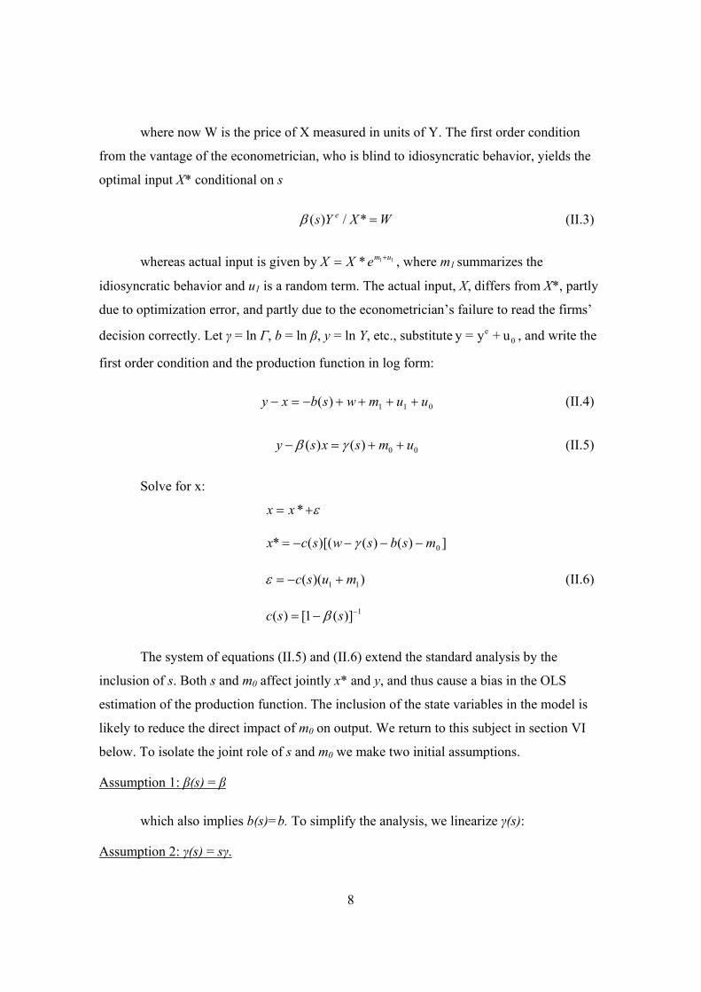
where now W is the price of X measured in units of Y. The first order condition

from the vantage of the econometrician, who is blind to idiosyncratic behavior, yields the

optimal input X* conditional on s

WXYs e =*/)(β (II.3)

whereas actual input is given by 11* umeXX += , where m1 summarizes the

idiosyncratic behavior and u1 is a random term. The actual input, X, differs from X*, partly

due to optimization error, and partly due to the econometrician’s failure to read the firms’

decision correctly. Let γ = ln Г, b = ln β, y = ln Y, etc., substitute 0e u+ y=y , and write the

first order condition and the production function in log form:

011)( uumwsbxy ++++−=− (II.4)

00)()( umsxsy ++=− γβ (II.5)

Solve for x:

ε+= *xx

])()()[((* 0msbswscx −−−−= γ

))(( 11 musc +−=ε (II.6)

1)](1[)( −−= ssc β

The system of equations (II.5) and (II.6) extend the standard analysis by the

inclusion of s. Both s and m0 affect jointly x* and y, and thus cause a bias in the OLS

estimation of the production function. The inclusion of the state variables in the model is

likely to reduce the direct impact of m0 on output. We return to this subject in section VI

below. To isolate the joint role of s and m0 we make two initial assumptions.

Assumption 1: β(s) = β

which also implies b(s)=b. To simplify the analysis, we linearize γ(s):

Assumption 2: γ(s) = sγ.

9

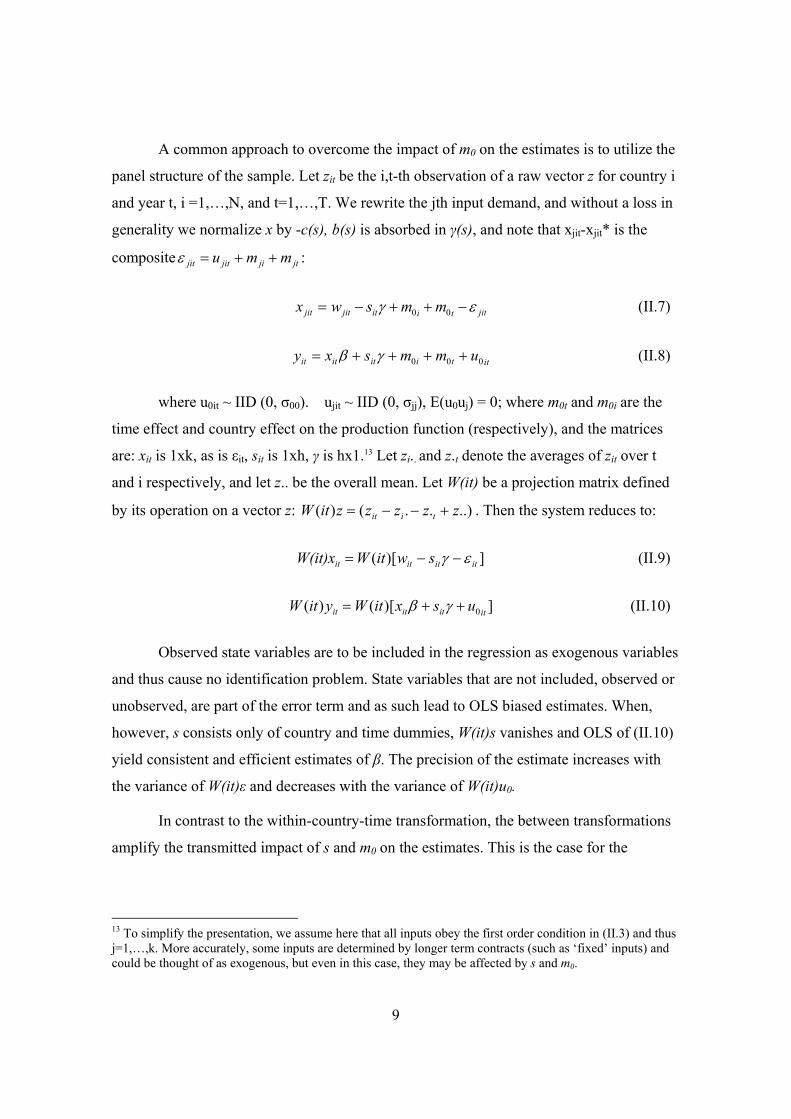
A common approach to overcome the impact of m0 on the estimates is to utilize the

panel structure of the sample. Let zit be the i,t-th observation of a raw vector z for country i

and year t, i =1,…,N, and t=1,…,T. We rewrite the jth input demand, and without a loss in

generality we normalize x by -c(s), b(s) is absorbed in γ(s), and note that xjit-xjit* is the

composite jtjijitjit mmu ++=ε :

jittiitjitjit mmswx εγ −++−= 00 (II.7)

ittiititit ummsxy 000 ++++= γβ (II.8)

where u0it ~ IID (0, σ00). ujit ~ IID (0, σjj), E(u0uj) = 0; where m0t and m0i are the

time effect and country effect on the production function (respectively), and the matrices

are: xit is 1xk, as is εit, sit is 1xh, γ is hx1.13 Let zi.. and z.t denote the averages of zit over t

and i respectively, and let z.. be the overall mean. Let W(it) be a projection matrix defined

by its operation on a vector z: ..)..()( zzzzzitW tiit +−−= . Then the system reduces to:

])[( itititit switWW(it)x εγ −−= (II.9)

])[( )( 0itititit usxitWyitW ++= γβ (II.10)

Observed state variables are to be included in the regression as exogenous variables

and thus cause no identification problem. State variables that are not included, observed or

unobserved, are part of the error term and as such lead to OLS biased estimates. When,

however, s consists only of country and time dummies, W(it)s vanishes and OLS of (II.10)

yield consistent and efficient estimates of β. The precision of the estimate increases with

the variance of W(it)ε and decreases with the variance of W(it)u0.

In contrast to the within-country-time transformation, the between transformations

amplify the transmitted impact of s and m0 on the estimates. This is the case for the

13 To simplify the presentation, we assume here that all inputs obey the first order condition in (II.3) and thus j=1,…,k. More accurately, some inputs are determined by longer term contracts (such as ‘fixed’ inputs) and could be thought of as exogenous, but even in this case, they may be affected by s and m0.

10

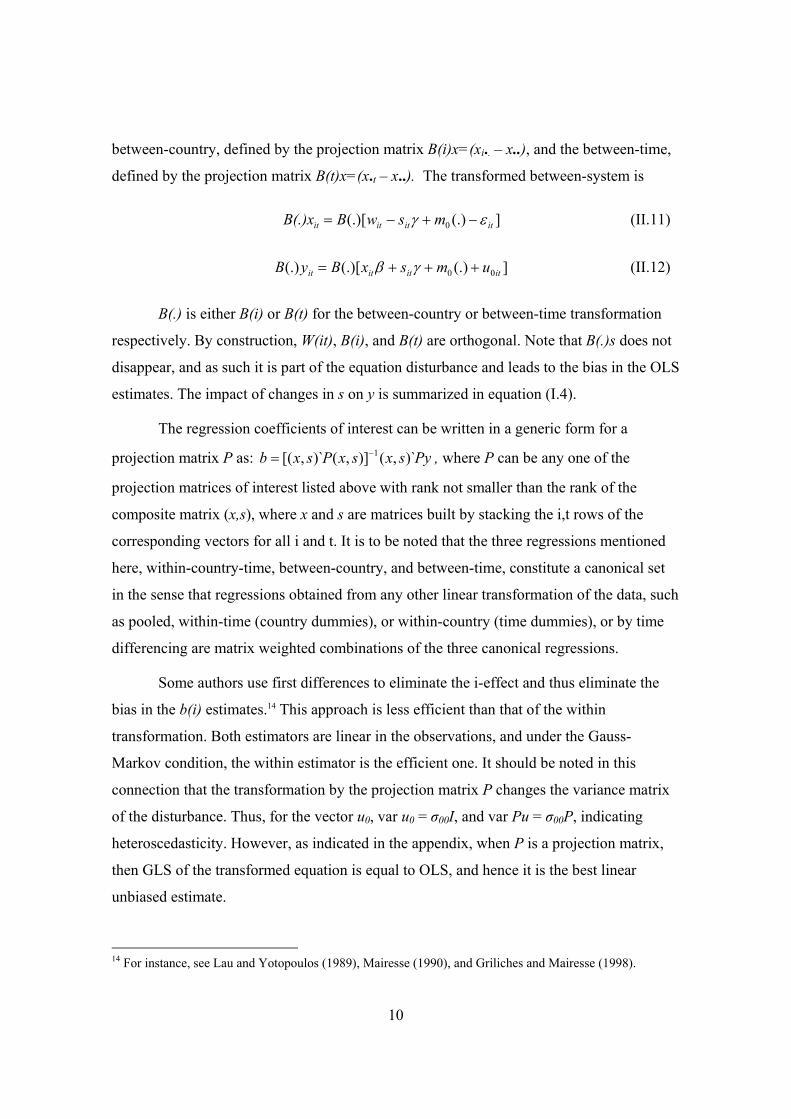
between-country, defined by the projection matrix B(i)x=(xi.. – x..), and the between-time,

defined by the projection matrix B(t)x=(x.t – x..). The transformed between-system is

](.)(.)[ 0 itititit mswBB(.)x εγ −+−= (II.11)

](.) (.)[ (.) 00 itititit umsxByB +++= γβ (II.12)

B(.) is either B(i) or B(t) for the between-country or between-time transformation

respectively. By construction, W(it), B(i), and B(t) are orthogonal. Note that B(.)s does not

disappear, and as such it is part of the equation disturbance and leads to the bias in the OLS

estimates. The impact of changes in s on y is summarized in equation (I.4).

The regression coefficients of interest can be written in a generic form for a

projection matrix P as: PysxsxPsxb )`,()],()`,[( 1−= , where P can be any one of the

projection matrices of interest listed above with rank not smaller than the rank of the

composite matrix (x,s), where x and s are matrices built by stacking the i,t rows of the

corresponding vectors for all i and t. It is to be noted that the three regressions mentioned

here, within-country-time, between-country, and between-time, constitute a canonical set

in the sense that regressions obtained from any other linear transformation of the data, such

as pooled, within-time (country dummies), or within-country (time dummies), or by time

differencing are matrix weighted combinations of the three canonical regressions.

Some authors use first differences to eliminate the i-effect and thus eliminate the

bias in the b(i) estimates.14 This approach is less efficient than that of the within

transformation. Both estimators are linear in the observations, and under the Gauss-

Markov condition, the within estimator is the efficient one. It should be noted in this

connection that the transformation by the projection matrix P changes the variance matrix

of the disturbance. Thus, for the vector u0, var u0 = σ00I, and var Pu = σ00P, indicating

heteroscedasticity. However, as indicated in the appendix, when P is a projection matrix,

then GLS of the transformed equation is equal to OLS, and hence it is the best linear

unbiased estimate.

14 For instance, see Lau and Yotopoulos (1989), Mairesse (1990), and Griliches and Mairesse (1998).

11

As the data generated by W(it) is cleaned from the time and country effects, they

should best represent the more stable technology, referred to here as the core implemented

technology.

III. Data 15

Output and inputs

We estimate a cross-country agricultural production function where agricultural

output depends on inputs, agricultural technology, and the state of the economy. In this

analysis we use a measure of agricultural capital which revises and updates the previously

constructed data set from Larson, Butzer, Mundlak, and Crego (2000). The inclusion of

agricultural capital is one of several aspects which differentiate this study from most

studies of agricultural production functions based on a panel of countries.

Agricultural output is measured as agricultural GDP in 1990 US dollars. We choose

the GDP variable rather than the more often used agricultural production because it comes

from the national accounts used for the construction of the fixed capital variable. Inputs to

agricultural production include land, capital, labor, and fertilizers. Hectares of agricultural

area are used for the measure of land. This includes arable land, land under permanent

crops, and permanent pastures. Agricultural labor is defined as the economically active

population in agriculture. Fertilizer consumption is often viewed as a proxy for the whole

range of chemical inputs. The data on agricultural capital consists of two components:

fixed capital, consisting primarily of structures and equipment, and capital of agricultural

origin, consisting of livestock and trees. The two components differ in the method of

construction, and also in terms of markets and pricing.

Technology

As the available technology is unobserved, what we can do in empirical analysis is

to identify variables associated with variations in the implemented technology. In the case

of agriculture, there is a natural variable to measure the level of technology for a given

15 For a description of the construction of the data, see Mundlak, Larson, and Butzer (1997). While the methodology is the same, sources have been updated and in some cases revised. Details can be obtained from the authors.

12

crop; this is the yield or output per unit of land. The yield has been the main criterion for

the introduction of the modern varieties of cereals and other crops, termed as the green

revolution, beginning around the middle of the last century. The higher is the yield of the

modern varieties, or the larger is the area devoted to these varieties, the larger is the

average yield. Extending this concept to aggregate output, we construct an aggregate peak

yield variable. For each country and each commodity, the maximum of the past yields is

computed, thereby reflecting the potential output from the implemented technology in any

given year. Country-specific Paasche indices (1990=1) are constructed of these peak

commodity yields, weighted by land area. A Paasche index is used since changing the

composition of output changes the relevance of existing technologies.

The most common variable used in empirical studies as a carrier or representative

of technology is some measure of human capital, mostly schooling. The basic idea is that

higher levels of education are conducive to technological progress.16 We include the

average schooling years of the total labor force, taken from Barro and Lee (2000).17

Empirical studies show the relevance of various public goods that are associated

with productivity, such as infrastructure in transportation and communication, measures of

public health, and research and extension.18 In this study we do not attempt to determine

the contribution of these variables individually, but rather allow for the overall effect of the

group on the estimation. We do this by selecting the per capita output in the country as a

comprehensive measure of capital and technology (Mundlak and Hellinghausen 1982). We

measure it as the ratio of the country per capita output to that of the United States and refer

to it as a development indicator. This variable replaces the need for introducing a dummy

variable to differentiate between developed and developing countries as some studies do.

16 However, the causality could go in either direction in that economic progress generates a demand for schooling. Therefore, the interpretation of a schooling variable in empirical analysis is somewhat ambiguous. 17 Education data are reported for every five years through the World Bank website (http://devdata.worldbank.org/edstats/). Data for other years are obtained through linear interpolations. 18 See for instance Evenson and Kislev (1975), Antle (1983), Binswanger et al. (1987), Lau and Yotopoulos (1989), and Craig, Pardey, and Roseboom (1997).

13

Institutions

It is assumed that the physical, legal, and regulatory infrastructure and institutions

support overall, including agricultural, development. We measure this influence with two

variables obtained from the Freedom House – political rights and civil liberties. The

measure of political rights reflects the electoral process, political pluralism and

participation, and functioning of the government. The civil liberties measure includes

aspects of freedom of expression and belief, associational and organizational rights, rule of

law, and personal autonomy and individual rights. Both measures are on a scale of 1 to 7,

where 1 represents the most free and 7 the least free. If these variables matter, they are

expected to be correlated with development and reflected in the development indicator.

They are nevertheless introduced here explicitly because of our interest in trying to isolate

the effects of institutions on agricultural productivity. Hence, the expected contribution of

these variables in the present analysis is over and above that of the development variable.

Incentives

We introduce two measures of incentives to allow for the direct effect of incentives

on productivity over and above their indirect effect through resource allocation and

accumulation. The measures are the terms of trade between the agricultural sector and the

overall economy, obtained as the relative price (agricultural GDP deflator to total GDP

deflator, lagged one period), and its variability, calculated as a moving standard deviation

from the three previous periods.19 Note that this measure confounds in it the various taxes

or subsidies, direct or indirect, applied to the sector. The variability in agricultural prices

reflects the market risk faced by agricultural producers. In addition to the sector-specific

risk, there is an economy-wide market risk, that of price volatility for the economy as a

whole, measured by the rate of inflation. This is calculated as the rate of change in the total

GDP deflator.

19 In an earlier paper, Mundlak, Larson, and Butzer (1999) used the price ratio of agriculture to that of manufacturing. The reason for the change is that the alternative to agricultural resources is not limited to manufacturing, but includes also services, which may, in fact, have become more important than manufacturing, particularly in developed countries.

14

Physical Environment

Agricultural production depends on the physical environment or natural conditions.

We represent the environment by using two variables: potential dry matter (PDM) and a

factor of water availability (FWA).20 The first variable is intended to measure the

theoretical potential production of dry matter. The production of dry matter requires

moisture. Arid areas may have a large value for PDM, but actual production is small due to

water deficit. The relative water availability is measured by the ratio of actual transpiration

to potential transpiration. These two variables are country specific and do not vary with

time.

IV. Sample description

The sample was determined by the data availability and the preference for a

balanced data panel in order to simplify the analysis. It consists of annual data from 30

countries21 for a 29-year period (1972-2000). The information conveyed by the sample is

summarized in Table 1. The first column presents the average annual growth rate of the

variables over the sample period. Agricultural output grew at a rate of 5.43 percent,

whereas agricultural capital grew at a higher rate of 5.77 percent. Agricultural labor

declined at the average rate of 0.6 percent. Thus, the average labor productivity increased

at the average rate of 6.03 percent, and the ratio of capital to labor increased at the average

rate of 6.37 percent. The growth rate of capital of agricultural origin (4.94 percent) is lower

than that of fixed capital (5.80 percent). Fertilizer grew on average at the rate of 1.87

percent, whereas the agricultural area grew at the rate of 0.01 percent, implying a growth in

the fertilizer-land ratio. The growth of agricultural output took place in spite of unfavorable

prices as indicated by the decline in the terms of trade of agriculture at the average rate of

1.26 percent. These results signal an increase in productivity. The technology measures

show a growth rate of schooling of 1.67 percent and 1.41 percent for peak yield.

20 The measures are based on Buringh, van Heemst, and Staring (1979) and were used in Mundlak and Hellinghausen (1982) and Binswanger et al. (1987). 21 Countries included in the study are: Australia, Austria, Canada, Cyprus, Denmark, Egypt, Finland, France, Greece, India, Indonesia, Italy, Kenya, Republic of Korea, Malawi, Mauritius, Morocco, Netherlands, Norway, Pakistan, Peru, Philippines, Sri Lanka, Sweden, Republic of Tanzania, Tunisia, Turkey, United Kingdom, United States, and Uruguay.

15

As mentioned above, the institutions measures are ordinal, and thus, growth rates

would be meaningless. To give a picture of how institutions have evolved over the time

period studied, we looked at the averages and medians of the indices for each year. For our

sample of countries, the average measure of civil liberties is 3.27 in 1972 and 2.57 in 2000.

For political rights, the averages are 3.17 and 2.37 respectively. Our sample covers

countries on both ends of the spectrum, with a few countries advancing from 6 and 7

(“non-free”) to 1 and 2 (“free”),22 while there are 7 countries which remain at 1 throughout

the time period.23

The qualitative nature of the above results is consistent with the common

knowledge on agricultural development in the sample period. The results are highlighted

here for two reasons: first to characterize the sample and second to show that the data are

subject to a great deal of variability over time and across countries. This variability

provides an insight into the relationships between the different variables of interest. To

describe the variability we decompose the total sum of squares to the three orthogonal

components (within-country-time, between-country, and between-time). Thus, SS total =

SS(xit - x..) is decomposed to SSW(it) = SS(xit - xi. - x.t + x..), SSB(i) = SS(xi. - x..), SSB(t)

= SS(x.t - x..), where, for any variable z, we use the notation: .z = SS(z) it2

ti∑∑

To standardize the results, we divide the components by the total sum of squares so

that the numbers in Table 1 show the percentage of each component in the total sum of

squares. The between-country differences account for most of the variability in output and

more so in the inputs; about 89 percent of the output variability is due to the between-

country differences. Thus, a regression which allows for a country effect, without any

quantitative variables, would yield an R2 of 0.89, so that the unexplained residual from

country averages accounts for only 11 percent of the total sum of squares of output. If we

add the time effect, the R2 rises to 0.98. Similarly, the between-country variability accounts

22 The terms “free, partially free and non-free” are used by Freedom House as classifications corresponding to the indices of political rights and civil liberties. 23 If we restrict the sample to countries which have at least one value not equal to 1, the range of averages increases to 4.09 and 3.14 for civil liberties and 4.10 and 2.95 for political rights (in 1972 and 2000 respectively).

16

for 95 percent to almost 100 percent of the total variability in land, labor, livestock, and

fertilizers. The situation is similar when the output and inputs are measured per worker.

The relative importance of the country and time components is different for the

variability of the state variables. The between-country component is important in

schooling, development, political rights, and civil liberties and less important in the other

variables. In part, this difference among the state variables reflects the way the variables

are measured. Schooling, development, political rights, and civil liberties are measured in

units that allow cross-country comparisons, and interestingly, the relative importance of

the between-country component in the total sum of squares is similar to that of output. We

can relate this discussion to the determinants of the inputs as shown in equation (II.6). It

seems that schooling, development, and the institutional variables can be identified with s

in that they are associated with the technology level and also affect the input level. They

seem to have a strong correlation with the country effect. On the other hand, the price

variables are indices, and as such, do not allow cross-country comparisons. They have a

strong deviation component and perhaps are associated with the allocation error. A strong

between-time effect is represented by the peak variable.

To sum up, the relative importance of the between-country component is dominant.

This can lead to the erroneous conclusion that the within analysis has little to contribute.

As a matter of principle, this conclusion is not well-founded because the precision of the

estimated coefficients depends not only on the spread in the regressors but also on the

variance of the equation disturbance which usually contains a component that is time

invariant. Consequently, the variance of the within component is considerably smaller than

the total variance. This is validated below where we show that the within estimates are

meaningful empirically and informative substantively.

V. Empirical results

Our ultimate interest is the estimation of the role of the inputs in production, or

simply the production elasticities. To do this we have to eliminate the jointness effect, or

the transmitted effect consisting of the state variables and of the country and time

idiosyncratic variables. To accomplish this we present here two models: the first is a pure

17

production function where inputs are the only regressors, and the second is an extended

function which contains also the state variables described in section III.

We organize the empirical results of each model in three blocks. The first block

presents the within-country-time estimates, b(it). The working hypothesis is that these

estimates are based on observations taken from the core technology. The second block

presents the between-time estimates, b(t), representing the time-series component, common

to all countries, and as such it captures the impact of changes over time in the available

technology. The last block presents the between-country estimates, b(i), summarizing the

between-country variability. The estimates are based on the locus of points that go across

the different techniques implemented by the countries which, in principle, operate under

the same available technology.

The general form of the estimated equation is:

it0it0 ))(())(())(( νγβγβγββ +++++++= bTitbTitbcitbcititit sxtBsxiBsxitWy (V.1)

where β0 is the intercept, and ittiit umm 0000 ++=ν .

Due to the orthogonal structure of the regressors, it is possible to estimate the three

blocks separately. We can do it by estimating (II.10) and (II.12), or by estimating (V.1).24

The difference will be in the dependent variable, and consequently in the value of R2 and

in the degrees of freedom used in the derivation of the t-score. We present the results from

both approaches for reasons to be discussed below.

Inputs only

The results are presented in Table 2. The dependent variable for columns termed

‘block’ is the transformed variable, Py, where P=W(it), B(t), and B(i) respectively,

associated with (II.10) and (II.12). The R2 and the t-score in the independent-block column

are obtained from this regression. The R2 appearing in the joint-block column is the

proportion of the total variability of y (not of Py) explained by this regression. The ratio of

the two values of R2 reflects the proportion of the block sum of squares in the total sum of 24 We refer to estimations of equations (II.10) and (II.12) as ‘independent-block’, while the estimation of equation (V.1) is termed ‘joint-block’.

18

squares of output, referred to as the weight. Thus, the R2 of the joint-block equation (V.1),

0.9566, is equal to the weighted average of the independent-block values for R2. The t-

score in the joint-block regression is obtained from the estimation of equation (V.1). It is

clear that the contribution of the within variables to the explanation of total output (y) is

relatively small and that the t-score of the coefficients is lower than that obtained from the

independent-block estimation where the dependent variable is W(it)y. On the other hand,

the difference between the two versions is smaller for the between-country estimates. This

is a demonstration of the consequences of an implicit or explicit preference for using the

between estimates, which in the case of panel data, would be the between-country

estimates. The within estimates are avoided by working with country averages. However,

the within variables provide information for identifying the production function and are

less contaminated by variables leading to inconsistency in the estimates.

The key question of this analysis is whether the coefficients of the variables

common to the three canonical regressions are the same, aside from sampling error. A

casual inspection of the results indicates that they are quite different, confirming the basic

initial hypothesis that the regressions summarize the combined effect of changes in inputs

and technology, and therefore the within and between regressions summarize different

processes.

To introduce uniformity in the results of the various models we impose constant

returns to scale on the within estimates. This constraint is imposed only on the within

estimates, because the between estimates are subject to the jointness effect and therefore do

not present pure input elasticities. The sum of the within elasticities without this constraint

is 1.25, and the difference between the input elasticities in the constrained and

unconstrained models is absorbed mostly in the land elasticity.25 The Wald test of constant

returns to scale in the within regression is not rejected at the 4 percent level.

The sum elasticities of the two types of capital is 0.42, and the elasticity of land is

0.33. With sum elasticities of 0.75 for capital and land, there is little scope left for labor

25 To save space we do not present the unconstrained results.

19

and fertilizer.26 This is the most important substantive result which indicates that

agriculture is capital-cost-intensive. The elasticity of fertilizers, 0.13, is considered to be

high for several reasons. First, we deal with the aggregate agricultural production function,

whereas fertilizer is used only on plant products. Thus the corresponding elasticity related

to the plant products should be higher than that obtained for the aggregate product. Second,

note that the dependent variable is value added, and in a competitive economy the

elasticity of fertilizer, whose cost is allowed for in the computation of value added, should

be nearly zero (an outcome of the envelope theorem). A higher value for the fertilizer

elasticity is likely to signal constraints on the supply of fertilizer causing the shadow price

to exceed the official price used in the national accounts to compute the cost of fertilizer.

The labor elasticity appears low, and we return to this subject later on. In Mundlak, Larson,

and Butzer (1999), the early literature on cross-country studies was reviewed, and it stands

out that our results differ from those reported in that literature. In part, it may be due to the

fact that we use a complete capital series, which was absent from the other studies, and in

part it is due to the fact that we use the within-time-country estimates, whereas the reported

results are mostly cross-country in nature and resemble the between-country regression in

the present study.

Turning to the between regressions, we note that the values of R2 are by far higher

than that of the within equation, and it is particularly high for the time-series component as

given in the between-time regression. The sum of the capital elasticities is 0.85 in the

between-time regression and 0.32 in the between-country regression. The between-time

elasticity is particularly high, and this suggests that the pace of the implementation of

changes in the available technology was strongly constrained by the level of the capital

stock in agriculture. Similarly, the land coefficient in the between-time regression is high,

but its t-score is low. A high value for the land coefficient suggests an increase in the

shadow price of land associated with the increase in productivity, while at the same time

there was little increase in the time series of agricultural area (Table 1).

26 These values are of the same order of magnitude obtained in an earlier study (Mundlak, Larson, and Butzer 1999) for a different sample of countries and different time period.

20

What is striking in the between-country regression is the low elasticity of land,

0.02, and the high elasticity of fertilizer, 0.41. This suggests that the techniques used by the

more productive countries were land-saving and fertilizer-using. The subject is taken up in

section VI.

The reduced form

The country and time effects are estimated as residuals, and the question is to what

extent they can be replaced by the state variables. The potential list of pertinent state

variables is of unknown length, but we can only deal with observed variables. To get an

idea on the relevance of our set of state variables, we estimate the reduced form of output,

equation (I.1), which in view of equation (I.4) amounts to a quasi-supply function, in the

sense that it allows for changes in the supply function. The state variables are decomposed

to their orthogonal components, and their impact on the estimates of the various blocks is

determined accordingly. The within estimates are determined by the interaction term,

W(it)s, and the between regressions are determined by B(.)s. The time behavior of the state

variables is demonstrated in Figure 1 which presents plots of the annual averages of B(t)s

over time. It is seen that schooling and peak yield show a positive trend and are highly

correlated (0.995). On the other hand, the relative prices and the price variability show a

negative trend. Civil liberties and political rights are also subject to negative trend, which

means overall improvements over time of these attributes. Inflation is fairly stable except

for a big jump around 1990.

The OLS results organized by blocks appear in Table 3.27 The values of the R2 are

not high for the within and the between-country regression in contrast to the time series.

This means that our variables capture well the changes over time, and less so for the cross

section. The R2 for the model as a whole is 0.613. Comparing these values to those in

Table 1, where the country effect by itself accounts for 89 percent of the output variance,

indicates that our set of state variables is far from coming close to being a perfect substitute

27 To save space, we present here t-scores only from the independent-block estimates.

21

for the country effects. The D.W. test statistic (2.171) is reported only for the between-time

regression, where it is relevant.28

It is obvious that the coefficients in the three blocks are different and therefore

represent different processes. Specifically, the relative price is positive and significant in

the within and the between-country regressions and negative in the between-time

regressions.29 The price variability has a negative coefficient in the within and in the

between-country regressions but not in the between-time regression. Schooling is positive

in all the three regressions, as is the development indicator. Civil liberties has the expected

negative sign in the within and between-time regression but not in the between-country

regression, while political rights has a negative coefficient in the between regressions, but

not in the within regression. Most of these results are carried over to the production

function with the state variables, referred to as the extended model.

To sum up, it is important to note that even though the within regression has a low

R2, it presents a supply function with expected signs. This is achieved by the interaction

terms W(it)s which are expected to cause input variations and to have a smaller impact on

the technology choice. This is not the case for the between regressions.

The extended production function

The OLS estimates of the extended model appear in Table 4. The R2 of this model

is 0.9694 as compared with 0.9566 in Table 2. This means that 29 percent of the

unexplained error of the model in Table 2 was reduced by the introduction of the state

variables. An F-test indicates that this addition is significantly different from zero.

Constant returns to scale is imposed on the within inputs elasticities. The sum elasticities

without this constraint is 1.22, and the difference between the constrained and

unconstrained elasticities is mostly in the elasticity of land.

An examination of the input elasticities shows that the big picture presented in

Table 2 has not changed in a dramatic way. Specifically, for the within estimates, the sum

28 We have also computed a principal components version. The results are not different in a substantive way from the OLS estimates and are therefore not reported here. 29 A similar result is reported in Binswanger et al. (1987).

22

elasticities of capital is 0.37 and the elasticity of land is 0.45, and this again leaves little

scope for fertilizer and labor. The input coefficients in the between-regressions are also

quite similar to those observed in Table 2. What then is the contribution of the state

variables to the within regression? The answer is the rise of R2, or the reduction of the

equation variance. To see where it comes from we first review the impact of the state

variables in the within block. The main contribution comes from the price block and the

development indicator. The price coefficient is positive and that of the price variability is

negative. This is consistent with a positive response to price changes and a negative one to

risk. In interpreting the role of price, we note that w which appears in the theoretical model

discussed above is the vector of real factor prices, which is unobserved. The relative price

in the regression is the terms of trade of agriculture, which is the denominator of the

components of the vector w. As we deal with the log of the price variables, the

denominator of the vector w can be separated from the nominal factor prices, and it is

introduced here explicitly into the equation. Thus the positive sign of the relative price

coefficient in the within regression is interpreted as a positive supply response of the

implemented technology. The price elasticity of productivity is 0.29, and that of the price

variability is -0.31. These are quite sizable values. Using a somewhat different

formulation, to which we return below, Fulginiti and Perrin (1993) reports a price elasticity

of productivity of 0.13.30

The development indicator, which reflects the overall infrastructure of the

economy, as well as the institutional and technological environment, seems to be the most

robust variable. This indicates that the more productive is the economy as a whole the

higher is the productivity of agriculture. The civil liberties variable has the anticipated

(negative) sign, whereas schooling has a weak negative impact. Note that the variables in

the within regression are the interaction after the main effects were extracted, and therefore

the sign indicates the correction to the influence of the variables as given by the main

effects.

The productivity response observed in the between regressions is not always

consistent with that of the within regression. In the between-country regression, the sign of

30 See also Hu and Antle (1993) and Binswanger et al. (1987) for price response in different formulations.

23

both the price and the price variability is the same as in the within regression. However, for

the between-time estimates, the price coefficients have the opposite signs, as the

productivity growth was associated with a decline in price and in a rise of the price

variability. This reflects a downward trend in the relative price associated with productivity

rise in world agriculture.

The price variability coefficient has a negative sign in the between-country

regression, indicating negative response to risk. Inflation has a negative coefficient in the

between-country regression.

The magnitude and the sign of the development indicator are robust across the three

equations. Schooling has a weak positive impact in the between regressions.31 The impact

of political rights and civil liberties is ambiguous and weak. The two physical environment

variables vary across countries but are time invariant. The sign of the water availability is

positive, as expected. The sign of potential dry matter is negative. This is inconsistent with

our earlier results and indicates that in this sample the high PDM countries were less

productive.

Stability of results

What happens when we remove the assumptions made in section II above? Assumption 2

of the linearity of γ(s) is not crucial and can be ignored here. Assumption 1 (constant β)

however, is more crucial. One way to find out the validity of this assumption is to run the

regression for subperiods. Table 5 presents results for two subperiods, 1972-1985 and

1985-2000.32 A comparison of the two periods, and with the results in Table 4 for the

whole period, indicates some changes but the qualitative nature of most of the main results

is preserved. The strength of the capital elasticities is preserved even though there is some

change in the composition of the two components of capital. The fertilizer elasticity is 0.14

and 0.13, and the interpretation of this value remains intact. The labor elasticity increased

in the second period. The rise in some of the elasticities reduces the elasticity of land, but

31 Because of the strong correlation between the time averages of schooling and peak yield, the latter variable is not included in the between-time regression. 32 We present here only the t-scores from the independent-block estimation. This is sufficient to establish the point of the dependence of the estimates on the period chosen.

24

still the sum elasticities of capital and land exceed 0.5. The rise in the elasticity of labor in

the second period may reflect the decline in the agricultural labor force.

Turning to the state variables, schooling has the wrong sign as before, but the peak

yield is positive and significant in the first period, which experienced a stronger rise in

yields. Finally, the role of price is positive and significant, whereas the price variability is

negative. Thinking of the within estimators as representing the core technology, we see

that the core technology is not detached from the economic environment and therefore is

not invariant to the sample.

The between-time regressions also preserve the important result of high elasticity

of capital. The sum elasticities of the two capital components are 0.94 for the first period,

0.70 for the second period as compared with 0.83 for the period as a whole. The between-

country estimates of the input elasticities show little change. The main changes are in the

coefficients of the state variables.

There are two possible approaches to incorporate the variability of β(s,x) in the

analysis.33 The first requires knowledge of the factor shares and consists of estimating the

elasticities from a system of factor shares and the production function.34 This approach has

problems of its own which are related to the interpretation we can give to the factor shares.

The second approach is to write out β(s,x) as a linear function of s and x which leads to a

quadratic production function in s and x.35 Such a function is blessed with many terms

which are intercorrelated and thus create a problem for the extraction of reliable results.

Note that the system reported in Table 4 already has a very high R2, and there is little scope

for squeezing in many additional terms. One possibility is to be selective with the number

of quadratic terms. For instance, Fulginiti and Perrin (1993) used the heterogeneous

technology framework to estimate such an equation including quadratic terms of the inputs

with some of the state variables (they refer to the state variables as technology-changing

variables) for a sample of 16 developing countries for the period 1961-1985. A key issue in

33 See Mundlak (1988, 2001). 34 See Mundlak, Cavallo, and Domenech (1989). 35 The dependence on x alone yields the translog function (Christensen, Jorgenson, and Lau 1973). We suppress here the dependence on x and concentrate the discussion on the dependence on s.

25

that study was to obtain a positive supply response to prices, and the outcome is an

elasticity of 0.13 for output price and -0.09 for wages.

VI. The role of the effects

Ordinarily, panel data analysis starts with the estimation of the coefficients of the

quantitative variables, and this is followed up with the introduction of discrete qualitative

variables, namely the effects. This natural course of action emphasizes the role of the

quantitative variables and diverts attention from the information embedded in the effects.

To clarify this point we can reverse the order and start the analysis by examining the role

of the effects. In our case this calls for the decomposition of the output sum of squares and

the computation of the R2 of an equation consisting solely of country and time dummies. In

our sample, such an equation explains about 98.5 percent of the total output sum of

squares, as shown in Table 1. All this, to be sure, is without an inclusion of any input in the

equation. But the inputs are there, because there is a strong correlation between the inputs

and the effects, and this goes back to the optimization described in equations (II.1) and

(II.2). As long as m0 affects the decision on input demand, the estimated effects reflect

input variations. For a similar reason they also reflect variations in the state variables.

The introduction of inputs to the empirical equation yields significant coefficients

but has little impact on the degree of explanation. The reason for this weak impact is that

the inputs are subject to strong country and time effects. These effects, however, do not

exhaust the input variability so that W(it)x does not vanish, and it is this remaining

variability that provides the information for the estimation of the coefficients.

To express the relationship between the effects and the regressors we rewrite

equation (V.1):

it00 ])[(])[( νππππγββ +++++++= sTitxTitscitxcitititit sxtBsxiBsxy (VI.1)

where γγπγγπββπββπ −=−=−=−= bTsTbcscbTxTbcxc ,, .

The within estimator provides an estimate of β and γ , whereas the between-

country and between-time estimators provide estimates of βbc, γbc, βbT, and γbT respectively.

Thus the π’s are the bias of the between estimators.

26

The relationship between the effects and the regressors is summarized by the

following equations

iscitxciti sxiBm 00 ])[( ςππ ++= (VI.2)

tsTitxTitt sxtBm 00 ])[( ςππ ++= (VI.3)

where ς 0i and ς 0t are the error terms.

An estimate of m0i and m0t is obtained from a regression of (II.8) with country and

time dummies. The values of R2 for the country regression (VI.2) are 0.554 with the state

variables alone, 0.830 with the inputs alone, and 0.885 for both groups. Similar regressions

for the time effect (VI.3) yield 0.982, 0.995, and 0.998 respectively. From this we learn

that the state variables account for most of the time effect and less so for the country effect.

The inputs account for a larger proportion of the country effect, but still less than of the

time effect. Technical change is the main event which evolved over time, and the set of the

state variables seems to be strongly correlated with it. The weaker relationship between the

state variables and the country effect indicates that there is a scope for introducing

additional state variables that are correlated with the country effect.

What are the implications of the estimates of equations (VI.2) and (VI.3)? The first

one is that it provides a set of variables that account for the effect. The set is not unique,

and we have already alluded to the long list of potential state variables used in the literature

to account for growth and productivity. Thus one would have to provide a rational for

preferring one set to an alternative one. The statistical analysis alone is insufficient to do

the task. The second implication is related to the estimation itself. Suppose that we have a

deterministic solution for the two equations, which means that we can replace the

unobserved effects with observed variables. How would it affect the estimation? The

answer is given by equation (VI.1). The estimate of β would be the within estimator, since

the unobserved effects represented by oim and otm and reflected in the π would vanish.

This means that explaining the effects can tell us something about how transformations of

the data affect bias related to unobservables, but it should not change our choice of

estimator.

27

VII. Evaluation

As there are big differences between the three estimators, it is desirable to get a

sense of reality and check how our estimates relate to the real world. We do it at a general

level, starting with the calculation of the TFP. Using the growth rates in Table 1 and the

within elasticities from Table 4 we obtain that TF increased at an average annual rate of

2.23 percent whereas TFP increased at an annual rate of 3.2 percent which accounts to 59

percent of output growth.

Using the elasticities, we compute the marginal value productivity, or shadow

price, as the product of the average value productivity and the corresponding elasticity.

Because the distribution is quite skewed, Table 6 presents the results of the median and of

the mean. We note that the shadow rate of return on fixed capital is quite high, and this is

consistent with the high growth rate of this input. Figure 2 presents the time path of the

median shadow prices from which we learn that the capital deepening resulted in

convergence to around 0.14. The shadow price of capital of agricultural origin is lower,

and this may be related to the way the variable was constructed. The shadow wage of labor

is relatively low which explains the migration of labor out of agriculture. The decline in

the labor force and the rise of capital caused the shadow wage to grow at the annual rate of

5.4 percent, considerably higher than that of TFP. There is a problem in comparing the

shadow wages to published wages. Published wages refer to payment for actual work,

whereas the labor data refer to the available labor force which is not fully occupied due to

the seasonality of farm work. This issue is discussed in some detail in a study on Asian

agriculture (Mundlak, Larson, and Butzer 2004). The shadow price of fertilizer increased

over time at a higher rate than that of TFP in spite of the fact that the fertilizer-land ratio

has increased constantly over time. Recall that the output is value added, and thus it is net

of fertilizer cost. It is likely that the price at the farm gate is higher than the price used in

national accounts, but still there may be a gap reflecting the rise in demand due to the shift

to fertilizer-intensive crops. Finally, the rent per hectare of land in 1990 dollar is 568 at the

mean and 271 at the median. To get from this to the value of land, we assume a

depreciation rate of 0.05 and subtract it from the shadow price of capital. We then

capitalize it by dividing the rent on land by the net rate of return to capital to obtain 2185

and 2464 1990 dollars per hectare at the mean and median respectively. There is of course

28

considerable variability in the sample as in reality. To sum up this evaluation, it seems that

our results have a realistic flavor which would not be the case if we repeated the

calculations with the between estimates.

VIII. Perspective

It is useful to relate the model briefly to the discussion in the literature on panel data.

1) Identification: The identification of the production function depends largely on the

allocation error. The more the firms deviate from the first order conditions, the more

accurate the estimates will be.

2) Consistency: In the absence of state variables, or under a weaker assumption where

W(it)s = 0, the OLS estimates of the within equation are consistent and those of the

between equations are not. Some authors use first differences to eliminate the i-effect in

order to eliminate the bias in the b(i) estimates.36 As indicated above, this approach is

inefficient.

3) Sample size: Increasing the sample size does not eliminate the bias caused by the

jointness effect; it only reduces the sampling error. This is true regardless of whether the

sample is increased through N or T (the number of countries or years).

4) Input spread: The decomposition of the sum of squares of the inputs show that SSB(i) is

dominating, and that SSW(it) is relatively small. It is, therefore, claimed that the within

estimator does not utilize important information. This is true but not the whole truth,

because SSW(it) also constitute a small fraction of the total SS of output. Thus, there is

less information, but there is less to be explained by this information. We have

demonstrated that the within estimator provides meaningful and statistically significant

results.

5) Fixed or random effects: The foregoing discussion is invariant to the assumption about

the nature of the idiosyncratic variables, or effects. Under the random effect model the

GLS estimator is a matrix-weighted average of the within and between estimators

(Maddala 1971), and it is therefore inconsistent. The source of the bias is the jointness

effect. 36 For instance, see Lau and Yotopoulos (1989) and Griliches and Mairesse (1998).

29

6) Measurement error: The within estimator is more sensitive to measurement errors.37 This

statement assumes implicitly that the measurement error is unaffected by the

transformation, so that its relative contribution to the within SS is larger than to the

between SS. This possibility is not ruled out, but it should be noted that there is good

reason to believe that part of the measurement error is country (or firm) specific, and by

the same token it is time specific, and is thus eliminated by the within transformation.38 It is

impossible to generalize on the relative importance of the measurement error in the

universe of all panels. What we learn from this study is that the most sensible results come

from the within transformation, and this transformation is consistent with the theory

formulated above.

7) Diversity of results: Concern has been expressed from the fact that there is a great deal

of diversity in the results obtained in production function estimates from panel data

depending on how the data are pooled (Griliches and Mairesse 1998; Mairesse 1990). The

diversity is a problem when the working hypothesis is that the estimates should be

invariant to way the data are pooled. The general model presented here indicates that one

should expect diversity, and in fact the diversity serves as a starting point for the

construction of more meaningful models.

8) Instrumental variables: The use of instrumental variables was suggested as a way to

overcome the bias in the estimates of panel data (Hausman and Taylor 1981). In the

present framework the scope for the use of instrumental variables is rather limited because

variables which are associated with the choice of inputs are assumed also to affect the

choice of the function itself. In other words, the instrumental variables fall in the category

of state variables in the present framework. The same argument also rules out the GMM

estimator.

9) Input ratios: In the Cobb-Douglas a difference between the log of two inputs,39 say j and

g, xjit – xgit, eliminates the terms m0 and, in the absence of state variables, can serve as an

37 See Griliches and Mairesse (1998). 38 For a fuller discussion, see Mundlak (2001). 39 See Mundlak (1996).

30

instrumental variable. In this approach, when the production function is estimated in terms

of average productivity, and constant returns to scale is imposed, the estimation is free of

the jointness bias. Unfortunately, under heterogeneous technology, this is no longer the

case.

IX. Summary and Conclusions

The paper presents an estimate of the agricultural production function from a panel of

countries.

1) Framework: In the world of heterogeneous technology, the implemented techniques and

inputs are jointly determined conditional on the state variables that are assumed to specify

the economic environment. Because of variability in the state variables, the production

function of a sector is an aggregate of micro production functions. It is approximated by a

Cobb-Douglas function with parameters that depend upon the state variables.

2) State variables enter as exogenous variables in the empirical equation, and the

estimation is straightforward when they are observed. In contrast, unobserved state

variables become part of the production function shock, thus creating a correlation between

the inputs and the productivity shocks, similar in nature to the transmission of the

idiosyncratic variables in panel data. Due to the structure of the problem, the only way to

identify the production function is through allocation errors, namely, through input

variations that are unaffected by the omitted state variables or the idiosyncratic

productivity shock.

3) The sum of squares of the panel data is decomposed into the three orthogonal

components. Most of the variability in output and inputs comes from between-country

variations, whereas the within-country-time variations account only for a small proportion

of the total sum of squares. Estimates obtained from between-country variations are

popular because they are based on a wide spread in the regressors. They are, however,

biased. On the other hand, the within-country-time variations of the inputs reflect largely

allocation errors and thus produce consistent or low-bias estimates.

4) When not all state variables are observed, the choice of regression matters. We provide

a practical example and present estimates obtained under the assumption of constant

31

slopes, for the canonical set of regressions, between-country, between-time (time-series

component), and within-country-time variations. There are great differences in the

estimates of the three canonical regressions. The elasticity of capital from the within

regression is 0.37, as compared to 0.27 from the between-country regression, and 0.83

from the between-time regression. The latter suggests that capital was a constraint in the

implementation of new capital-intensive techniques, in spite of the fact that capital grew

faster than all other inputs and output. These numbers are indicative of the differences in

the results obtained from the three regressions, and similar differences exist for the other

variables. The elasticity of fertilizer from the within regression is 0.1, although it should be

close to zero because output is measured by GDP, which is net of fertilizer costs. This

indicates that the shadow price of fertilizer was higher than the market price. However, the

value obtained for the fertilizer coefficient from the between-country regression is 0.44. If

this were a true elasticity, it would mean that 44 percent of GDP should be attributed to

fertilizer; clearly, this is absurd. In contrast, it is likely that land is a dominant factor of

agricultural production. In this case, the elasticity of land in the between-country

regression is 0.03 as compared to 0.45 in the within regression. These comparisons provide

substantive evidence on the superiority of the within estimator. This is true even in

comparison to linear estimates obtained from pooled data, since these are weighted matrix-

averages of the three canonical regressions and reflect the bias of their components.

5) Agriculture: The new techniques were capital and fertilizer intensive. This is reflected in

the growth rates of these inputs. On the other hand, the techniques were labor saving; this

is consistent with the decline in the size of the labor force in agriculture. The land elasticity

is high for the within and the time component, and low for the between countries. Thus, the

more productive countries use land-saving and fertilizer-using techniques. The land

elasticity reflects the terms of trade of agriculture for the period, which, on the whole,

enjoyed important improvements in productivity. The decomposition of output growth

shows that TFP accounted for 59 percent of the output growth of 5.43 percent.

6) State variables: The relevance of the state variables was tested by estimating the reduced

form, or a quasi-supply function. They account for most of the variability of the between-

time output, and only slightly for the within output. Still the within regression provides a

supply function with the right signs and significant coefficients. Turning to the production

32

function, the relative price of agriculture has a positive impact, and its variability has a

negative impact in the within regression. The development indicator indicates that the

agricultural productivity is positively correlated with the strength of the economy as a

whole. The indicator is assumed to represent total capital, physical and human, and the

institutional infrastructure. Some of the variables which are confounded in the indicator

were introduced explicitly into the regression, but their contribution was marginal.

7) Accounting for the effects: The country and time effects account for most of the

variability in the data. It is shown that the effects are embedded in the country and time

means of the inputs and the state variables. The state variables are particularly important in

capturing the time effect, and less so for the country effect. This suggests that there is a

scope for trying out additional state variables to account for the cross-country variations.

8) Stability of results: The estimates are sensitive to the economic environment. This is

demonstrated by estimating the regressions for two sub-periods. Even though the estimates

change, the main message is preserved.

10) The results are consistent with the changes that take place in the process of growth.

Agricultural productivity rises, there is a shift to capital and fertilizer-intensive and labor-

extensive techniques. The response in resource allocation leads to growth in the marginal

productivities of labor, fertilizer, and land, and a slight decline in the marginal productivity

of capital as a result of the fast growth of the capital-labor ratio. From the point of view of

growth, policies should encourage the process to continue.

33

Appendix

Equivalence of OLS and GLS estimators:

Following Zyskind (1967), Rao (1973), Baltagi (2006), we state the following theorem:

Theorem: Let y=Xβ + u, where u ~ (0, V).

OLS and GLS of β are equal if and only if there exists a matrix B such that VX = XB.

We apply the theorem as follows:

Consider the transformation Py = (PX) β + Pu, where Pu ~(0, σ2P)

Check the condition of the theorem: VPX = σ2PX = PXσ2

Thus the matrix σ2I is the matrix B of the theorem.

This theorem explains why we continue to apply OLS to equations which are premultiplied

by projection matrices.

34

Bibliography

Acemoglu, Daron, Simon Johnson, and James Robinson, “Institutions as the Fundamental Cause of Long-Run Growth” (pp. 385-472), in Philippe Aghion and Steven N. Durlauf (Eds.), Handbook of Economic Growth Volume 1A (Amsterdam and San Diego: Elsevier, North-Holland, 2005).

Antle, John M., “Infrastructure and Aggregate Agricultural Productivity: International Evidence,” Economic Development and Cultural Change 31:3 (1983), 609-619.

Baltagi, Badi H., “An Alternative Derivation of Mundlak’s Fixed Effects Results Using System Estimation,” Econometric Theory 22:6 (2006), 1191-1194.

Barro, Robert J., and Jong-Wha Lee, “International Data on Educational Attainment: Updates and Implications,” CID Working Paper No. 42 (2000).

Barro, Robert J., and Jong-Wha Lee, “Sources of Economic Growth,” Carnegie-Rochester Conference Series on Public Policy 40 (1994), 1-46.

Barro, Robert J., and Rachel M. McCleary, “Religion and Economic Growth Across Countries,” American Sociological Review 68:5 (2003), 760-781.

Binswanger, Hans P., Yair Mundlak, Maw-Cheng Yang, and Alan Bowers, “On the Determinants of Cross-Country Aggregate Agricultural Supply,” Journal of Econometrics 36:1/2 (1987), 111-131.

Buringh, P., H. D. J. van Heemst, and G. J. Staring, “Computation of the Absolute Maximum Food Production of the World,” Wageningen: Netherlands Department of Tropical Soil Science, 1975; also published in H. Linneman et al. (Eds.) Moira Model of International Relations in Agriculture (Amsterdam: North-Holland Publishing Co., 1979).

Chamberlain, Gary, “Multivariate Regression Models for Panel Data,” Journal of Econometrics 18:1 (1982), 5-46.

Christensen, Laurits R., Dale W. Jorgenson, and Lawrence J. Lau, “Transcendental Logarithmic Production Frontiers,” Review of Economics and Statistics 55:1 (1973), 28-45.

Cobb, Charles W., and Paul H. Douglas, “A Theory of Production,” American Economic Review 18:1 supplement (1928), 139-165.

Craig, Barbara J., Philip G. Pardey, and Johannes Roseboom, “International Productivity Patterns: Accounting for Input Quality, Infrastructure, and Research,” American Journal of Agricultural Economics 79:4 (1997), 1064-1076.

Dollar, David, “Outward-Oriented Developing Economies Really Do Grow More Rapidly: Evidence from 95 LDCs, 1976-1985,” Economic Development and Cultural Change 40:3 (1992), 523-544.

Durlauf, Steven N., and Danny T. Quah. “The New Empirics of Economic Growth” (pp. 235-308) in John B. Taylor and Michael Woodford (Eds.), Handbook of Macroeconomics Volume 1A (Amsterdam; New York and Oxford: Elsevier Science, North-Holland, 1999).

35

Durlauf, Steven N., Paul Johnson, and Jonathan R. W. Temple, “Growth econometrics” (pp. 555-677), in Philippe Aghion and Steven N. Durlauf (Eds.), Handbook of Economic Growth Volume 1A (Amsterdam and San Diego: Elsevier, North-Holland, 2005).

Easterly, William, and Ross Levine, “It's Not Factor Accumulation: Stylized Facts and Growth Models,” World Bank Economic Review 15:2 (2001), 177-219.

Evenson, Robert E., and Yoav Kislev, “Investment in Agricultural Research and Extension: A Survey of International Data,” Economic Development and Cultural Change 23:3 (1975), 507-521.

Frankel, Jeffrey A., and David Romer, “Does Trade Cause Growth?” American Economic Review 89:3 (1999), 379-399.

Fulginiti, Lilyan E., and Richard K. Perrin, “Prices and Productivity in Agriculture,” The Review of Economics and Statistics 75:3 (1993), 471-482.

Griliches, Zvi, and Jacques Mairesse, “Production Functions: the Search for Identification” (pp. 169-203), in Steinar Ström (Ed.), Econometrics and economic theory in the 20th century: the Ragnar Frisch Centennial Symposium (Cambridge University Press, New York, 1998).

Hall, Robert E., and Charles I. Jones, “Why Do Some Countries Produce So Much More Output Per Worker Than Others?” Quarterly Journal of Economics114:1 (1999), 83-116.

Hausman, Jerry A., and William E. Taylor, “Panel Data and Unobservable Individual Effects,” Econometrica 49:6 (1981), 1377-1398.

Henderson, Daniel J., and R. Robert Russell, “Human Capital and Convergence: A Production-Frontier Approach,” International Economic Review 46:4 (2005), 1167-1205.

Hu, Fan, and John M. Antle, “Agricultural Policy and Productivity: International Evidence,” Review of Agricultural Economics 15:3 (1993), 495-505.

Klenow, Peter J., and Andres Rodriguez-Clare, “The Neoclassical Revival in Growth Economics: Has it Gone Too Far?” (pp. 73-103), in Ben S. Bernanke and Julio Rotemberg (Eds.), NBER Macroeconomics Annual 1997 (Cambridge, MA: MIT Press, 1997).

Larson, Donald F., Rita Butzer, Yair Mundlak, and Al Crego, “A Cross-Country Database for Sector Investment and Capital,” World Bank Economic Review 14:2 (2000), 371-391.

Lau, Lawrence, and Pan A. Yotopoulos. “The Meta-Production Function Approach to Technological Change in World Agriculture,” Journal of Development Economics 31:2 (1989), 241-269.

Maddala, G. S., “The Use of Variance Components Models in Pooling Cross Section and Time Series Data,” Econometrica 39:2 (1971), 341-358.

36

Mairesse, Jacques, “Time -Series and Cross-Sectional Estimates on Panel Data: Why are They Different and Why Should They Be Equal?” (pp. 81-95), in Joop Hartog, Geert Ridder, and Jules Theeuwes (Eds.), Panel data and labor market studies (Amsterdam: North-Holland, 1990).

Mankiw, N. Gregory, David Romer, and David N. Weil, “A Contribution to the Empirics of Economic Growth,” Quarterly Journal of Economics 107:2 (1992), 407-437.

Marschak, Jacob, and William H. Andrews, Jr., “Random Simultaneous Equations and the Theory of Production,” Econometrica 12:3/4 (1944), 143-205.

Mundlak, Yair. “Endogenous Technology and the Measurement of Productivity” (pp. 316-331), in Susan M. Capalbo and John M. Antle (Eds.), Agricultural Productivity: Measurement and Explanation (Washington, D.C.: Resources for the Future, 1988).

Mundlak, Yair, “On the Empirical Aspects of Economic Growth Theory,” American Economic Review 83:2 (1993), 415-420.

Mundlak, Yair, “Production Function Estimation: Reviving the Primal,” Econometrica 64:2 (1996), 431-438.

Mundlak, Yair, “Production and Supply” (pp. 3-85), in Bruce L. Gardner and Gordon C. Rausser (Eds.), Handbook of Agricultural Economics Volume 1A, Agricultural Production (Amsterdam; London and New York: Elsevier Science, North-Holland, 2001).

Mundlak, Yair, Domingo Cavallo, and Roberto Domenech, “Agriculture and Economic Growth, Argentina 1913-84,” Research Report 76 (Washington, D.C.: International Food Policy Research Institute, 1989).

Mundlak, Yair, and Rene Hellinghausen, “The Intercountry Agricultural Production Function: Another View,” American Journal of Agricultural Economics 64:4 (1982), 664-672.

Mundlak, Yair, and Irving Hoch, “Consequences of Alternative Specifications in Estimation of Cobb-Douglas Production Functions,” Econometrica 33:4 (1965), 814-828.

Mundlak, Yair, Donald F. Larson, and Rita Butzer, “The Determinants of Agricultural Production: A Cross-Country Analysis,” Policy Research Working Paper 1827 (Washington, D.C.: The World Bank, 1997).

Mundlak, Yair, Donald F. Larson, and Rita Butzer, “Rethinking within and between Regressions: The Case of Agricultural Production Functions,” Annales d'Economie et de Statistique 55-56 (1999), 475-501.

Mundlak, Yair, Donald F. Larson, and Rita Butzer, “Agricultural Dynamics in Thailand, Indonesia and the Philippines” Australian Journal of Agricultural and Resource Economics 48:1 (2004), 95-126.

North, Douglass C., Institutions, Institutional Change and Economic Performance (Cambridge; New York and Melbourne: Cambridge University Press, 1990).

37

Presbitero, Andrea F., “Institutions and Geography as Sources of Economic Development,” Journal of International Development 18:3 (2006), 351-378.

Pritchett, Lant, “Understanding Patterns of Economic Growth: Searching for Hills among Plateaus, Mountains, and Plains,” World Bank Economic Review 14:2 (2000), 221-250.

Rao, C. R., Linear Statistical Inference and its Applications (New York: John Wiley & Sons, 1973).

Rodrik, Dani, Arvind Subramanian, and Francesco Trebbi, “Institutions Rule: The Primacy of Institutions over Geography and Integration in Economic Development,” Journal of Economic Growth 9:2 (2004), 131-165.

Sachs, Jeffrey D., and Andrew M. Warner, “Fundamental Sources of Long-Run Growth,” American Economic Review 87:2 (1997), 184-188.

Sala-i-Martin, Xavier, Gernot Doppelhofer, and Ronald I. Miller, “Determinants of Long-Term Growth: A Bayesian Averaging of Classical Estimates (BACE) Approach,” American Economic Review 94:4 (2004), 813-835.

World Bank, World Development Report 2008: Agriculture for Development (Washington, D.C.: The World Bank, 2007).

Zyskind, George, “On Canonical Forms, Non-Negative Covariance Matrices and Best and Simple Least Squares Linear Estimators in Linear Models,” The Annals of Mathematical Statistics 38:4 (1967), 1092-1109.

38

TABLE 1: GROWTH RATES AND THE DECOMPOSITION OF THE SUM OF SQUARES Average Annual Decomposition of the Sum of Squares Growth Rate (expressed as a percentage of total) Variable (%) SSB(t) SSB(i) SSW(it) Output GDP 5.43 9.00 89.47 1.54 Inputs Capital 5.77 8.84 88.62 2.54 Fixed capital 5.80 6.60 91.03 2.37 Capital of agricultural origin 4.94 5.50 91.94 2.55 Livestock 3.59 3.09 95.72 1.18 Orchards 5.77 4.13 93.35 2.53 Agricultural area 0.01 0.00 99.93 0.07 Labor -0.60 0.07 99.03 0.90 Fertilizer 1.87 1.01 96.47 2.53 Technology Schooling 1.67 7.32 88.05 4.63 Peak yield 1.41 79.37 6.30 14.33 Development indicator 1.10 95.46 3.44 Institutions Political rights 1.57 79.28 19.16 Civil liberties 1.17 82.67 16.16 Prices Relative prices -1.26 25.01 23.14 51.85 Price variability 11.06 27.34 61.60 Inflation 3.12 8.50 88.37 Per Labor Output and Inputs GDP 7.93 90.12 1.95 Capital 6.71 90.41 2.88 Fixed capital 4.59 92.87 2.54 Capital of agricultural origin 6.74 89.80 3.46 Livestock 3.58 94.17 2.25 Orchards 7.53 88.35 4.11 Agricultural area 0.09 99.13 0.78 Fertilizer 1.11 97.72 1.18

39

TABLE 2: PRODCUTION FUNCTION, INPUTS ONLY Within time-country Between time Between country Variable Estimate t-score Estimate t-score Estimate t-score Block Joint Block Joint Block Joint Inputs Fixed capital 0.34 18.83 8.75 0.70 77.47 5.95 0.27 19.16 16.79 Capital of agricultural origin 0.08 4.11 1.91 0.15 13.62 1.05 0.05 5.81 5.09 Agricultural area 0.33 5.01 17.12 1.32 0.02 2.52 2.21 Fertilizer 0.13 5.51 2.56 -0.07 -5.37 -0.41 0.41 24.37 21.35 Labor 0.12 3.17 1.47 -1.10 -21.67 -1.67 0.17 24.57 21.53 Sum of estimates 1.00 0.93

Summary statistics Joint regression

Panel R-squares R-square Weight R-square Weight R-square Weight R-square 0.957 0.015 0.384 0.090 0.997 0.895 0.962 Durbin-Watson statistic 1.088

40

TABLE 3: REDUCED FORM PRODUCTION FUNCTION, STATE VARIABLES ONLY Independent block regressions Variable Within time-country Between time Between country Estimate t-score Estimate t-score Estimate t-score Technology Schooling 0.26 4.89 1.20 12.86 0.54 3.50 Peak yield 0.10 0.82 11.27 8.25 Institutions Civil liberties -0.03 -2.85 -0.48 -14.61 2.38 20.68 Political rights 0.02 2.00 -0.04 -1.00 -1.42 -17.56 Development indicator 0.96 12.60 1.79 20.38 2.50 8.73 Price block Relative prices 0.34 9.77 -1.72 -18.86 12.46 25.01 Price variability -0.39 -3.40 2.09 10.49 -26.78 -16.77 Inflation 0.00 1.44 -0.05 -6.76 -0.30 -5.14 Environmental Potential dry matter -0.76 -3.91 Factor of water availability -0.54 -3.50

Joint regression

Summary statistics R-square Weight R-square Weight R-square Weight R-square Panel R-squares 0.613 0.015 0.280 0.090 0.977 0.895 0.582 Durbin-Watson statistic 2.171 .

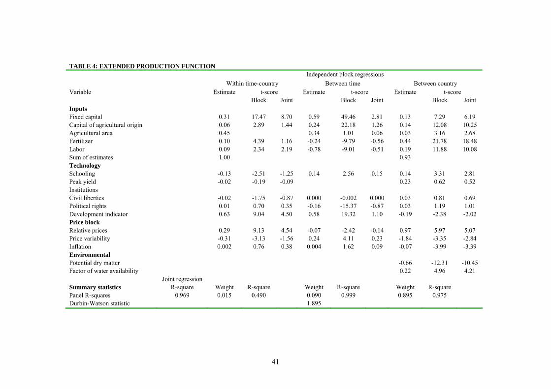
41

TABLE 4: EXTENDED PRODUCTION FUNCTION Independent block regressions Within time-country Between time Between country Variable Estimate t-score Estimate t-score Estimate t-score Block Joint Block Joint Block Joint Inputs Fixed capital 0.31 17.47 8.70 0.59 49.46 2.81 0.13 7.29 6.19 Capital of agricultural origin 0.06 2.89 1.44 0.24 22.18 1.26 0.14 12.08 10.25 Agricultural area 0.45 0.34 1.01 0.06 0.03 3.16 2.68 Fertilizer 0.10 4.39 1.16 -0.24 -9.79 -0.56 0.44 21.78 18.48 Labor 0.09 2.34 2.19 -0.78 -9.01 -0.51 0.19 11.88 10.08 Sum of estimates 1.00 0.93 Technology Schooling -0.13 -2.51 -1.25 0.14 2.56 0.15 0.14 3.31 2.81 Peak yield -0.02 -0.19 -0.09 0.23 0.62 0.52 Institutions Civil liberties -0.02 -1.75 -0.87 0.000 -0.002 0.000 0.03 0.81 0.69 Political rights 0.01 0.70 0.35 -0.16 -15.37 -0.87 0.03 1.19 1.01 Development indicator 0.63 9.04 4.50 0.58 19.32 1.10 -0.19 -2.38 -2.02 Price block Relative prices 0.29 9.13 4.54 -0.07 -2.42 -0.14 0.97 5.97 5.07 Price variability -0.31 -3.13 -1.56 0.24 4.11 0.23 -1.84 -3.35 -2.84 Inflation 0.002 0.76 0.38 0.004 1.62 0.09 -0.07 -3.99 -3.39 Environmental Potential dry matter -0.66 -12.31 -10.45 Factor of water availability 0.22 4.96 4.21 Joint regression Summary statistics R-square Weight R-square Weight R-square Weight R-square Panel R-squares 0.969 0.015 0.490 0.090 0.999 0.895 0.975 Durbin-Watson statistic 1.895

42

TABLE 5: EXTENDED PRODUCTION FUNCTION BY SUB-PERIODS Within time-country Between time Between country 1972-1985 1985-2000 1972-1985 1985-2000 1972-1985 1985-2000 Independent block regression Estimate t-score Estimate t-score Estimate t-score Estimate t-score Estimate t-score Estimate t-score Inputs: Fixed capital 0.38 10.29 0.43 14.38 0.80 50.84 0.76 42.72 0.11 4.78 0.18 6.64 Capital of agricultural origin 0.20 5.54 0.07 2.83 0.14 9.85 -0.06 -4.54 0.14 8.39 0.16 10.67 Agricultural area 0.15 0.06 7.55 12.76 -6.55 -28.98 0.01 0.07 0.01 0.55 Fertilizer 0.14 4.38 0.13 3.83 0.40 9.08 0.10 7.18 0.42 17.01 0.42 14.61 Labor 0.13 1.41 0.31 4.92 0.54 2.08 -1.12 -5.71 0.29 13.21 0.21 10.17 Sum of estimates 1.00 1.00 0.98 0.97 Technology: Schooling -0.04 -0.48 -0.22 -2.19 -0.29 -2.50 0.26 2.30 -0.002 -0.04 -0.05 -0.85 Peak yield 0.67 4.61 -0.54 -2.83 -0.64 -2.53 -1.80 -2.00 Institutions: Civil liberties -0.04 -3.14 -0.01 -0.74 0.04 1.74 -0.08 -10.64 0.07 1.93 -0.32 -6.76 Political rights 0.01 1.02 -0.01 -0.96 -0.02 -1.06 0.16 13.61 0.01 0.26 0.18 5.28 Development indicator 0.26 2.72 0.48 5.22 -0.50 -6.30 0.74 19.85 0.34 2.81 -0.50 -4.79 Price block: Relative prices 0.23 5.82 0.39 7.24 0.64 14.09 -0.39 -10.61 0.08 0.63 -0.36 -1.62 Price variability -0.26 -2.62 -0.53 -3.25 0.31 9.35 -0.33 -3.40 1.77 3.70 -0.84 -1.05 Inflation 0.04 0.70 -0.001 -0.67 -0.40 -13.78 0.003 2.00 0.08 0.67 0.003 0.27 Environmental: Potential dry matter -0.60 -7.69 -0.61 -8.98 Factor of water availability 0.18 2.57 0.21 3.22 Summary Statistics Weight R-square Weight R-square Weight R-square Weight R-square Weight R-square Weight R-square R-squares 0.012 0.546 0.013 0.569 0.031 1.000 0.020 0.999 0.957 0.977 0.967 0.973 Durbin-Watson statistic 3.443 2.499 Joint regressions 1972-85 1985-2000 R-square 0.973 0.968 Number of observations 420 480

43

TABLE 6: PRODUCTIVITY EVALUATIION Growth decomposition Marginal products

Growth rate Elasticity Contribution Mean Median Growth rate of median value

Factors Fixed capital 5.80 0.31 1.80 0.31 0.16 -0.37 Capital agricultural origin 4.94 0.06 0.30 0.06 0.04 0.49 Area 0.01 0.45 0.00 568 271 5.43 Fertilizer 1.87 0.10 0.19 1,468 1,097 5.24 Labor -0.60 0.09 -0.05 911 307 6.03 Total Factors 2.23 Productivity 3.20 Output 5.43

44

FIGURE 1: STATE VARIABLES

-.3

-.2

-.1

.0

.1

.2

.3

72 74 76 78 80 82 84 86 88 90 92 94 96 98 00

SCHOOLING

-.20

-.15

-.10

-.05

.00

.05

.10

.15

.20

72 74 76 78 80 82 84 86 88 90 92 94 96 98 00

PEAK YIELD

-.4

-.3

-.2

-.1

.0

.1

.2

.3

.4

72 74 76 78 80 82 84 86 88 90 92 94 96 98 00

CIVIL LIBERTIES

-.4

-.3

-.2

-.1

.0

.1

.2

.3

.4

.5

72 74 76 78 80 82 84 86 88 90 92 94 96 98 00

POLITICAL RIGHTS

-.12

-.08

-.04

.00

.04

.08

72 74 76 78 80 82 84 86 88 90 92 94 96 98 00

DEVELOPMENT INDEX

-.3

-.2

-.1

.0

.1

.2

.3

72 74 76 78 80 82 84 86 88 90 92 94 96 98 00

RELATIVE PRICE

-.04

-.02

.00

.02

.04

.06

.08

72 74 76 78 80 82 84 86 88 90 92 94 96 98 00

PRICE VARIABILITY

-0.4

0.0

0.4

0.8

1.2

1.6

2.0

72 74 76 78 80 82 84 86 88 90 92 94 96 98 00

INFLATION

45

FIGURE 2: MEDIAN MARGINAL PRODUCTS

.11

.12

.13

.14

.15

.16

.17

.18

.19

.20

72 74 76 78 80 82 84 86 88 90 92 94 96 98 00

FIXED CAPITAL

.028

.032

.036

.040

.044

.048

72 74 76 78 80 82 84 86 88 90 92 94 96 98 00

LIVESTOCK AND ORCHARDS

100

200

300

400

500

600

700

72 74 76 78 80 82 84 86 88 90 92 94 96 98 00

AGRICULTURAL AREA

400

600

800

1000

1200

1400

1600

1800

2000

72 74 76 78 80 82 84 86 88 90 92 94 96 98 00

FERTILIZER

0

200

400

600

800

1000

1200

72 74 76 78 80 82 84 86 88 90 92 94 96 98 00

LABOR

46