heterogeneous risk and time preferences - home - … procedure based on a hierarchical bayes...

J Risk Uncertain (2016) 53:1–28DOI 10.1007/s11166-016-9243-x

Heterogeneous risk and time preferences

Alina Ferecatu1 ·Ayse Onculer2

Published online: 14 November 2016© The Author(s) 2016. This article is published with open access at Springerlink.com

Abstract Assessing individuals’ time and risk preferences is crucial in domainssuch as health-related decisions (e.g., dieting, addictions), environmentally-friendlypractices, and saving opportunities. We propose a new method to jointly elicit andestimate risk attitudes and intertemporal choices. We use a novel individual levelestimation procedure based on a hierarchical Bayes methodology, which can inte-grate different functional forms for discounting and risk attitudes. This methodprovides individual level estimates, and allows us to explore the heterogeneity inthe data. In addition, we report a negative correlation between risk and time prefer-ences, implying that risk-seeking individuals are less patient and less willing to deferconsumption.

Keywords Risk and time · Risk preferences · Intertemporal choice · Jointelicitation · Hierarchical Bayes · Heterogeneity

JEL Classifications D81 · D90 · C11

Electronic supplementary material The online version of this article(doi:10.1007/s11166-016-9243-x) contains supplementary material, which is available to authorizedusers.

� Alina [email protected]

Ayse [email protected]

1 Rotterdam School of Management, Erasmus University, Burgemeester Oudlaan 50, 3062PA,Rotterdam, The Netherlands

2 ESSEC Business School, 1 Avenue Bernard Hirsch, 95000, Cergy, France

http://crossmark.crossref.org/dialog/?doi=10.1007/s11166-016-9243-x&domain=pdf

http://dx.doi.org/10.1007/s11166-016-9243-x

mailto:[email protected]

mailto:[email protected]

2 J Risk Uncertain (2016) 53:1–28

1 Introduction

When making decisions in an intertemporal setting, individuals are known to heav-ily discount future outcomes and to have a strong preference for immediate gains(Loewenstein and Prelec 1992; Frederick et al. 2002). Understanding individuals’intertemporal decisions and designing tools to improve their decision making processhas been a major research concern, with individual welfare and public policy impli-cations. Are people myopic about health decisions such as following better diets,quitting smoking, or exercising? Do public policy makers respond appropriately tothe threat of global warming, a decision involving a tradeoff between short termexpenses and long run rewards? Chesson and Viscusi (2003) analyze the joint influ-ence of time and uncertainty and conclude that people may have difficulties choosingthe optimal precautionary measures to prevent climate change, a long term hazard,due to both ambiguity in the probability of global warming phenomena and also dueto the ambiguity in the timing of global warming consequences. This suggests thata joint model of risk and time preferences is necessary to assess decision makers’tradeoffs between outcomes at different points in time.

The current study proposes a methodology that jointly elicits and estimates riskand time preferences at the individual level. We elicit risk attitudes and intertemporalchoices following Holt and Laury’s (2002) risk aversion experimental procedure andColler and Williams’s (1999) time discounting methodology involving price lists. Weembed a constant relative risk aversion specification in an exponential discountingmodel, following Andersen et al. (2008). Our main contribution is methodological.We add a layer of flexibility to the estimation method through a hierarchical Bayesmethodology, which allows us to recover individual level estimates and assess the het-erogeneity in intertemporal choices and risk attitudes. Hierarchical Bayes modelingis a validated alternative to maximum likelihood estimation (Rossi et al. 2005; Toubiaet al. 2013). The flexibility of the method in dealing with highly non-linear modelspecifications represents an important benefit. Such individual level estimates can beused in simulation studies to assess the effectiveness of changes in public policy deci-sions. To our knowledge, this is the first study that uses hierarchical Bayes modelingto jointly estimate risk and time preferences and to analyze the heterogeneity in thedata.

Our results suggest that individuals are generally risk-averse, with a mean constantrelative risk aversion coefficient of 0.515; their discount rates are in line with previousfindings on joint elicitation (mean discount rate of 12%). The methodology is generaland can be adapted to different functional forms. To test the robustness of our results,we estimate time preferences by using an exponential model, a hyperbolic modelproposed by Mazur (1987), another hyperbolic specification by Prelec (2004), and amixture model that allows a part of the population to behave as exponential discoun-ters, and the remaining part as hyperbolic discounters. Our study provides evidencethat controlling for the curvature of the risk aversion leads to lower estimated dis-count rates in experiments with hypothetical stakes. We conduct a clustering studyand find three types of decision makers based on their risk and time preferences:

J Risk Uncertain (2016) 53:1–28 3

a high patience type (risk-averse, low discounting), a moderate patience type (withaverage risk and time preferences), and a low patience cluster (risk-seeking, highdiscounting). This result suggests that regulators could design policy interventionsspecifically aimed at people with various degrees of patience. The increased reliabil-ity of our estimates also allows us to revisit the issue of the correlation between riskand time preferences. We find evidence that risk-seeking people are more impatientand require higher interest rates to postpone consumption.

The remainder of the paper is organized as follows. In the next section, wepresent a brief literature review on joint elicitation and estimation of risk and timepreferences. The experimental procedure for the joint elicitation of risk and time pref-erences is introduced in Section 3. In Section 4, we introduce our empirical modeland present the estimation methodology involving a hierarchical Bayes approach. InSection 5, we report the results from our Bayesian estimation and further investigatethe heterogeneity of risk and time preferences via individual differences and clustersof decision makers. The paper concludes with a discussion and the implications ofour findings.

2 Existing literature

Recent developments in the intertemporal choice literature include a joint elicitationof risk and time preferences (Andersen et al. 2008; Laury et al. 2012; Andreoni andSprenger 2012a; Toubia et al. 2013). This stream of literature emerged based on theconjecture that eliciting time preferences while assuming risk neutrality leads to anoverestimation of discount rates. Using multiple price lists, Andersen et al. (2008)jointly elicit subjects’ risk attitudes and intertemporal choices and show that dis-count rates are significantly lower than those reported in previous studies and more inline with market rates (10.1% on average). In another study, Andreoni and Sprenger(2012a) ask subjects to allocate a convex budget over a specific time period and findan average implied discount rate of 30% per year. They also observe that time prefer-ences are generally dynamically consistent. Using a binary lottery mechanism, Lauryet al. (2012) propose an elicitation of discount rates that corrects for the non-linearity,and is invariant to the form of the utility function. Their elicitation method yieldssimilar results to the joint elicitation of time and risk preferences in Andersen et al.(2008), with an average discount rate of 12.2% per year. These results show that it iscrucial to consider individuals’ risk attitudes when eliciting time preferences in orderto prevent an overestimation of discount rates.

The studies mentioned above as well as some other experimental findings(Kimball et al. 2009; von Gaudecker et al. 2011; Cardenas and Carpenter 2013) reportsignificant heterogeneity in risk attitudes and intertemporal choices. Andersen et al.(2008) analyze the heterogeneity caused by observable individual characteristics aswell as unobservable characteristics and find evidence for unobserved heterogene-ity. Meyer (2013) reports substantive heterogeneity in time preferences for publicgoods, heterogeneity that cannot be explained by observable personal characteristics.


However, Chesson and Viscusi (2000) show that several individual differencevariables impact time discounting. Nonsmokers and people with a post-graduate edu-cation degree have higher discount rates than smokers and subjects without advancededucation. This highlights the challenge of designing a model of decision makingunder risk and time that can accommodate individual level behavior.

Several studies in behavioral decision making analyze the heterogeneity in thedata and propose individual level parameter estimates. For instance, Jarnebrant et al.(2009) and Nilsson et al. (2011) estimate prospect theory parameters using hierar-chical Bayes methods. A recent study by Toubia et al. (2013) focuses on building adynamic (adaptive) survey design similar to conjoint studies, which presents decisionmakers with a personalized set of choices to elicit their risk and time preferences.They estimate cumulative prospect theory parameters as well as a quasi-hyperbolictime discounting model via a hierarchical Bayes procedure. They capture the hetero-geneity in parameter values and use it for estimation and for designing the adaptivequestionnaires.

Although essential for building theoretical and empirical models in decision mak-ing, as well as for public policy, the correlation between risk aversion and discountrate has received relatively little attention. Experimental studies on risk and timepreferences have traditionally focused on one of the two phenomena apart from fewexceptions. Andersen et al. (2008) report a small but significant positive correla-tion between subjects’ attitudes toward risk and time, such that the level of discountrates increases with their risk aversion. Their findings are supported by evidence inAnderhub et al. (2001). Anderson and Stafford (2009) find that individuals becomeless patient as risk increases. Abdellaoui et al. (2013) report a small negative corre-lation between risk aversion and impatience for gains, in one of the two experimentsthey conducted. In a second experiment, they find no relation between risk aversionand impatience. Moreover, as utility over time and utility under risk are different,Abdellaoui et al. (2013) suggest using two utility functions, a risk function to trans-form risky prospects into certainty equivalents, and a time discounting function torecover the present value of the certainty equivalent. These contradictory results sug-gest that further assessment of the correlation between risk and time preferences isnecessary.

3 Experimental design

We elicit risk and time preferences using the joint elicitation method proposed byAndersen et al. (2008).1 The reason for choosing this methodology is twofold. First,we are interested in implied discount rates and our goal is to eliminate confoundsintroduced by the utility curvature that lead to upwards bias when estimating time

1The experimental procedure can be found in the Online Appendix, and is thoroughly documented inAndersen et al. (2008).


preferences. Second, the methodology is more pliable to our hierarchical Bayes spec-ification, allowing us to obtain reliable individual level estimates of risk and timepreferences.

We recruited subjects by sending an invitation email to MBA and M.Sc. studentsfrom a large French business school. Students were invited to attend the experimentduring their lunch break, and were offered multiple time slots. While student samplesare prevalent in decision making research, the literature raises issues related to thegeneralizability of the results to the overall population. Our subjects are enrolled in abusiness school and 96.5% of them have taken at least one finance related course priorto participating in the experiment. Thus, they seem to be more financially educatedthan the average population. Falk et al. (2013) study the behavior of student samplesversus a representative sample of the general population and conclude that there is noconcern for self-selection bias among students, and students’ behavior does not seemto be significantly different than that of the general population. Our experimentalresults are in line with Laury et al. (2012), who employ an undergraduate studentsample from a large US university. Andersen et al. (2008) use a representative sampleof the adult Danish population and report an average discount rate lower than in ourexperiment. Andreoni and Sprenger (2012a) report a higher discount rate than all theabove cited studies, with an undergraduate freshman and sophomore sample.

A total of 87 students participated in the experiment, in exchange for course credit.Subjects were informed that once the experiment is over, a lottery would be held, and5 winners would receive a e20 gift voucher for a large media retailer. Subjects werenot informed of the likely number of participants in the experiment, and were there-fore not able to compute their chances of winning the lottery. The experiment beganwith the experimenter reading the instructions aloud. Participants were asked to turnto their computer screens and complete two tasks, the discount rate task and the riskaversion task. Subjects did four risk aversion tasks and four time discounting tasks,and completed a questionnaire about their age, gender, major, and their grade in theintroductory finance course, if they had attended one. After completing the experi-mental task, subjects were debriefed and told that they would be informed about theresults of the lottery within a month. Each experimental session took about 30 min-utes. We conducted 21 experimental sessions, with about five subjects per session, toensure sufficient attention from the experimenter to read the instructions and provideanswers to questions.

3.1 Identifying risk preferences

The experimental procedure used to identify subjects’ risk preferences is based onthe Holt and Laury (2002) risk aversion experiment. Each subject is presented with achoice between two lotteries A and B. Table 1 shows the payoff matrix presented tothe subjects. In the first decision line, lottery A offers a 10% chance of wining e200and a 90% chance or winning e160. The respondents did not see the expected valuesof the lotteries or the constant relative risk aversion (CRRA) intervals. In Table 1, wecan see that the expected values of lottery B increase relative to the expected values


Table 1 Typical payoff matrix in the risk aversion experiment. Subjects were asked to complete four riskaversion tasks with different payoffs, in the same income range

Open CRRA interval

Lottery A Lottery B EV(A) EV(B) Difference if subject switches

p e p e p e p e e e in e to lottery B

0.1 200 0.9 160 0.1 385 0.9 10 164 47.5 116.5 −∞ −1.71

0.2 200 0.8 160 0.2 385 0.8 10 168 85 83 −1.71 −0.95

0.3 200 0.7 160 0.3 385 0.7 10 172 122.5 49.5 −0.95 −0.49

0.4 200 0.6 160 0.4 385 0.6 10 176 160 16 −0.49 −0.15

0.5 200 0.5 160 0.5 385 0.5 10 180 197.5 −17.5 −0.15 0.14

0.6 200 0.4 160 0.6 385 0.4 10 184 235 −51 0.14 0.41

0.7 200 0.3 160 0.7 385 0.3 10 188 272.5 −84.5 0.41 0.68

0.8 200 0.2 160 0.8 385 0.2 10 192 310 −118 0.68 0.97

0.9 200 0.1 160 0.9 385 0.1 10 196 347.5 −151.5 0.97 1.37

1 200 0 160 1 385 0 10 200 385 −185 1.37 ∞

of lottery A, as one goes down the table. If a subject is indifferent between the twooptions, she can specify her indifference by choosing option I. The logic behind therisk aversion task implies that only very risk-seeking individuals will choose lotteryB in the first row and only very risk adverse individuals will choose lottery A in therow before last. Risk neutral subjects are expected to switch to lottery B at decisionrow 5. The last row is a consistency check, as all subjects are bound to prefer lotteryB, which strictly dominates lottery A.

For the sake of comparison, the relative payoffs are kept the same as in Andersenet al. (2008), but we divide the payoffs by 10 to remain in the income range overwhich we intend to estimate subjects’ risk aversion.

3.2 Identifying time preferences

Our experimental design for eliciting time preferences is based on the multiple pricelists introduced by Coller and Williams (1999). We follow similar time intervals asin Andersen et al. (2008), to be able to compare the two methodologies. We use fourintertemporal choice tasks by manipulating the time when the rewards are offered tosubjects (t=2 months, 6 months, 1 year and 2 years for option B). Table 2 is an exam-ple of the payoff table given to the subjects in order to elicit their time preferences.Subjects are asked to choose between option A and option B. If a subject is indiffer-ent, she can choose option I, for indifference. Option A offerse300 in one month andoption B offers e(300 + x) six months from now, where x is computed given a dis-count rate of 5% to 50% on the principal of e300, compounded quarterly. We use acompounded interest rate to increase ecological validity; in practice, a year or a quar-ter is the most common compounding period.We use the latter because in the first two


Table 2 Payoffs table for the 6-month time horizon in the discount rate experiment. Subjects completedfour intertemporal choice tasks, with different time horizons (t=2 months, 6 months, 1 year and 2 yearsfor option B)

Payment Payment Annual Annual Preferred

Payoff Option A Option B Interest Effective Payment

(amount (e) (amount (e) Rate Interest Rate Option

Alternative to be paid to be paid (AR) (AER) (Choose A,

in 1 month) in 6 months) I or B)

1 300 306.17 5% 5.09% A I B

2 300 312.40 10% 10.38% A I B

3 300 318.68 15% 15.87% A I B

4 300 324.99 20% 21.55% A I B

5 300 331.36 25% 27.44% A I B

6 300 337.78 30% 33.55% A I B

7 300 344.25 35% 39.87% A I B

8 300 350.76 40% 46.41% A I B

9 300 357.32 45% 53.18% A I B

10 300 363.92 50% 60.18% A I B

time discounting tasks, the experimental time frames are less than a year. The eliciteddiscount rates lie within a specific interval. For instance, for the choices available inTable 2, if a subject chooses option A in decision row 3 and option B in decisionrow 4, her discount rate lies in the interval (15%, 20%). Given that subjects completefour intertemporal choice tasks, our estimation method can infer stable interest ratesthat may lie inside an interval, not only at the interval bounds. We present subjectswith annual and annual effective interest rates,2 to facilitate comparison with otheropportunities for investment present outside the lab and minimize errors in judgment.

We introduce a one-month delay for option A for all tasks to avoid quasi-hyperbolic discounting (Laibson 1997). There is extensive evidence in the economicsand psychology literatures that individuals exhibit a bias for immediate payoffs. Dis-count rates elicited from choices between a current payoff and a future one aresignificantly higher than the discount rates elicited from two future choices. Oneexplanation for such present biased preferences is a preference for certain outcomes(Andreoni and Sprenger 2012b). Subjects would disproportionately prefer the cer-tain present option to the inherently risky future option. Since this present bias is notthe focus of our study, we introduced a front-end delay. In our experiment, subjectschoose between two future payoffs and they are expected to behave as exponentialdiscounters (Andreoni and Sprenger 2012b). Delaying both options also reduces theinfluence of transaction costs on intertemporal choices. If only the delayed option

2These terms are explained in the experimental instructions (see the Online Appendix).


involved greater transaction costs, the revealed discount rate would include these sub-jective costs. As both options occur in the future, such transaction costs are equivalentand will not influence the revealed discount rate.3

3.3 Consistency and validity checks

Our experiment involves hypothetical stakes. The literature presents mixed evidenceon whether individuals respond differently to hypothetical choices involving risk ortime discounting than they do in a real-choice context. Taylor (2013) shows thaton average, measured risk preferences are not significantly different across real andhypothetical settings. Holt and Laury (2002) demonstrate that individuals appear tobe more tolerant of risk in a hypothetical setting, and that this “hypothetical bias”increases with the size of the stakes. Camerer (2004) notes that the effect of incen-tives on behavior is likely to depend on the task. However, the choice over moneygambles is not likely to be a domain in which people would behave according toexpected utility theory if they put more effort into the task. Using functional mag-netic resonance imaging (fMRI), Kang et al. (2011) show that common areas of thebrain are activated when individuals make real and hypothetical choices about thepurchase of consumer goods, but that the level of this activity differs.

In our experiment, we provided the subjects with a sample task before the exper-iment to ensure that they understood the instructions clearly (one decision row waschosen from both time discounting and risk preference tasks). We also performeda consistency check for the first time discounting and risk aversion tasks (see theOnline Appendix). Few subjects switched between lotteries A and B in either tasks.Subjects switched back to lottery A after choosing lottery B in only 1.7% of therisk aversion tasks (6 tasks out of 348 completed) and in 3.7% of the time discount-ing elicitations (13 tasks out of 348 completed). Furthermore, no subject chose onlyoption A or only option B throughout the four time discounting or risk aversion tasks,suggesting that subjects’ risk and time preferences are within the ranges provided inthe experimental design.

To assess the quality of our data, we conducted a within-subject analysis in the fourrisk aversion and time discounting tasks. After computing the variance in switchingpoints, we averaged the standard deviation across subjects. On average, the switchingpoint between the smaller, sooner and larger, later payoffs varied by 1.66 decisionrows. For the risk preferences task, the switching point varied on average by 1.09decision rows. The switching point varied significantly more for the discount ratetasks than for the risk aversion tasks (p < 0.01). This variation is not only due toresponse error, but also due to hyperbolic discounting, i.e. subjects tend to be morepatient, thus switch at a lower decision row, as the time interval increases. Eventhough most subjects chose to switch from lottery A to lottery B without selecting theoption corresponding to an indifference point (79.04% for risk aversion tasks, 69.5%for the discounting tasks), the relatively large number of stated indifference points

3We note that the two-month delay for option B in the first intertemporal choice task occurred during thesummer vacation. This could have led to an increase in reported discount rates.


(20.96% for the risk elicitation task and 30.5% for the discounting task) helped us toestimate the discount rates and risk aversion coefficients, by improving the precisionof the recovered estimates.

4 Model specification

Our hierarchical Bayes framework provides a natural context in which we jointlyestimate individual level risk and time preferences. We set up 1) a risk preferencespecification, 2) a method to jointly measure risk and time preferences, and 3) amethod to capture heterogeneity in individual preferences. We review all the threecomponents in turn.

4.1 Modeling risk preferences

We do not impose any assumptions about linear risk preferences in income.Consequently, the utility function is the constant relative risk aversion (CRRA)specification (Holt and Laury 2002):

U(M) = (ω + M)(1−r)

1 − r, f or r �= 1 (1)

where M is the monetary amount, ω is the time invariant amount of backgroundconsumption, and r is the CRRA coefficient where r = 0 denotes risk neutral behav-ior, r > 0 denotes risk aversion and r < 0 denotes risk-seeking behavior. Thebackground consumption represents estimated daily consumption levels, assumedconstant over the time frame we analyze. Given our CRRA specification and positivevalues of background consumption, as opposed to ω=0, observed choices from ourexperiment imply higher levels of risk coefficients, thus more curvature of the utilityfunction. We assume positive levels of background consumption as in Andersen et al.(2008) and exogenously vary its value to provide a sensitivity analysis of our resultsto the level of estimated daily consumption.

To specify the likelihood of the risk aversion responses, we first compute theexpected utility (EU) as the sum of payoffs weighted by the probabilities induced bythe experimenter. Given that there are two outcomes (k=1, 2) in each lottery j, the EUfor each lottery is:

EUj =∑

k=1,2

p(Mk) × U(ω + Mk) (2)

Following Holt and Laury (2002), we implement a simple stochastic specification tospecify the likelihood conditional on the model. The specification is standard in thedecision making literature and has been implemented by Andersen et al. (2008) andLaury et al. (2012).

� EU = EU1μ

B

EU1μ

B + EU1μ

A

(3)

where �EU is the cumulative probability distribution reflecting differences in theexpected utility of the two lotteries A and B and μ is a behavioral noise parameter.


When μ → 0, the specification collapses to the deterministic expected utility theory(EUT), where the alternative with the highest expected utility will be chosen withcertainty. However, when μ → ∞, the choices become random, indifferent to theexpected utilities. Toubia et al. (2013) introduce a similar error specification, wherea noise parameter implies whether choices are random or whether they converge to adeterministic selection.

The likelihood of the risk aversion responses conditional on EUT and CRRAspecification depends on r and μ. The conditional log-likelihood is:

lnLRA(r, μ, y, ω) =∑

j

{[ln(�EU)|yj = 1] + [12ln(�EU) +

+1

2ln(1 − �EU)|yj = 0] + [ln(1 − �EU)|yj = −1]}(4)

where yj = 1 implies the choice of option B; yj = −1 the choice of option Aand yj = 0 shows indifference between A and B, implying a 50-50 mixture of thelikelihood of choosing either of the lotteries.

4.2 Modeling time preferences

We first consider the mainstream specification of time preferences. Assumingexponential discounting, a subject is indifferent between two income options if:

U(ω + Mt) + 1

(1 + δ)τU(ω) = U(ω) + 1

(1 + δ)τU(ω + Mt+τ ) (5)

where U(ω + Mt) is the utility of monetary outcome Mt for delivery at time t plusbackground consumption ω; δ is the discount rate; τ is the delay to the larger, laterreward.

The utility function U(.) is separable and stationary over time. The left-hand sideof Eq. 5 is the sum of the discounted utilities of receiving the monetary outcome Mt

at time t (in addition to background consumption) and receiving nothing extra at timet+τ , and the right-hand side is the sum of the discounted utilities of receiving nothingover background consumption at time t and the outcome Mt+τ (plus backgroundconsumption) at time t + τ .

The specification we use for the discount rate is similar to the one employed forrisk aversion. By assuming the CRRA utility function as before, we can write thediscounted utilities of each of the two options as:

PVA = 1

(1 + δ)tU(ω + MA) + 1

(1 + δ)t+τU(ω) (6)

PVB = 1

(1 + δ)tU(ω) + 1

(1 + δ)t+τU(ω + MB) (7)

where PVA and PVB are the present values of option A and option B; MA and MB

are the monetary amounts in the discounting tasks presented to subjects, to be paid attime t and time t + τ respectively.


The cumulative distribution function for the discount rate task is specifiedsimilarly as for risk aversion.

� PV = PV1ν

B

PV1ν

B + PV1ν

A

(8)

where �PV is the cumulative probability distribution reflecting differences in thepresent values of the two tasks, conditional on r, δ and ν. ν is the behavioral noiseparameter, allowing some subjects to make some errors from the perspective ofexpected utility theory, similar to the μ noise parameter in the risk aversion task.Given that the risk aversion task involves choices in lotteries as opposed to values,we assume that it is cognitively more difficult, therefore expect μ > ν.

The log-likelihood for the time discounting responses, conditional on r, δ and ν,is:

lnLDR(r, μ, δ, ν, y, ω) =∑

j

{[ln(�PV )|yj = 1] + [12ln(�PV ) +

+1

2ln(1 − �PV )|yj = 0] + [ln(1 − �PV )|yj = −1]}

(9)

where yj = -1, 1 and 0 denotes selection of option A, B or indifference in observationj, respectively.

The joint likelihood of the risk aversion and the discount rate responses can thenbe written as:

lnL(r, μ, δ, ν, y, ω) = lnLRA + lnLDR (10)

4.3 The hierarchical Bayes specification: Heterogeneity and priors

The most common approach in estimating decision making models (cumulativeprospect theory, time discounting etc.) is single-subject maximum likelihood estima-tion (MLE). There are several limitations of using a single-subject MLE methodol-ogy. First, while the method is efficient when a large number of observations persubject are available, its main drawback is the assumption that all subjects are inde-pendent, without considering that individual parameter estimates originate from agroup-level distribution. The hierarchical Bayes estimation simultaneously estimatesthe individual level parameters and addresses the above limitation through a compro-mise between the two extremes of complete independence and pooling (average-levelparameter estimates where all subjects are presumed to be identical). The methodshrinks the individual estimates towards the group mean, and this effect is morepronounced when the individual estimates are less reliable.

Second, the single-subject MLE provides point estimates for the model param-eters. Using these point estimates in analyses of variance or regressions, withoutfactoring in their reliabilities, could lead to poor predictions, as results can be severelyinfluenced by extreme observations. Through the above mentioned shrinkage effect,


the hierarchical Bayes estimation provides a way to directly quantify the uncer-tainty on the parameters. Thus, it prevents unreliable information from having adisproportionate influence on the parameter estimates.

A random effects approach (or an error components approach—formally equiv-alent) allows for correlation in unobserved utility over several choices for eachrespondent, and overcomes the assumption of complete independence. Since such amodel usually involves high-dimensional integrals that are analytically intractable,the random effects model is estimated via maximum simulated likelihood (MSLE),or Bayesian methods. In addition to the simulation step necessary to integrate overall values of the model parameters for each individual, MSLE also involves an opti-mization step, leaving it vulnerable to issues such as reach of global maxima vs. localmaxima, and requires a tolerance level and proper starting values. Bayesian inferenceis a simulation technique that can overcome such problems, because it covers theparameter space more effectively (see Jackman 2009 for proofs involving hierarchi-cal specifications). The quantities of interest in Bayesian inferences are the posteriordistributions of the model parameters, and the method provides an exact estimationof these distributions, in small as well as in large samples (Rossi and Allenby 2003).MSLE provides an approximation of these distributions, and needs large samples forasymptotic properties of convergence. Relevant for our setting, the Bayesian infer-ence is more suited than MSLE to ensure that all parameters have the same sign orare bounded within a certain range for all subjects. The Bayesian procedure handlestransformations of the model parameters more efficiently (e.g., exponential transfor-mation for log-normally distributed parameters), as it does not search for a maximum.The method is particularly suited in situations where only a limited amount of dataper subject are available for a moderately large sample of subjects, typical for exper-iments in decision making. It provides reliable estimates even with a small amountof data per individual (Rossi and Allenby 2003).

Using Bayes’ theorem, we combine the likelihood function in Eq. 10 with priordistributions to obtain posterior distributions for our model parameters. The twobuilding blocks of our Bayesian framework are related to the specification of hetero-geneity and the introduction of prior distributions of the parameters. We introduceeach of the aspects in turn.

We estimate individual level parameters by leveraging the information on the dis-tribution of parameters across subjects in our experiment. We specify the followingheterogeneity model:

θi = θ0 + ui; ui ∼ N(0, Vθ ) (11)

where θi is the vector of individual level risk and time coefficients (ri , δi , μi, νi). θ0represents a vector of average risk and time preferences and related noise parameters.The unexplained heterogeneity, ui , is normally distributed. Vθ shows the variance ofthe model parameters and the covariances between them. This matrix, along with thecorrelation between the individual level risk and time estimates, allows us to assessthe link between subjects’ risk attitudes and intertemporal choices.

Our model is a hierarchical Bayes model because we formulate prior distributionsnot only on the parameters that specify the likelihood function, but also on those


priors themselves. We set up a two-stage model that allows the first-stage priors tobe influenced by the data. The prior on θi , usually referred to as a first-stage prior,follows a normal distribution:

First-stage prior

θi ∼ N(θ0, Vθ )

To ensure the parameters remain in an acceptable range, i.e., δi, μi, νi are positive-definite, we apply an exponential transformation to the parameter estimates. We alsoset priors on the parameters in the heterogeneity model, called second-stage priors.

Second-stage prior

vec(θ0|Vθ) ∼ N(θ0, A−1 ⊗ Vθ)

Vθ ∼ IW(ν, V0)

The second-stage priors would allow us to incorporate any information that wemight have before our data collection. These priors are usually chosen to be as unin-formative as possible, to allow the data to determine the values of the parameterestimates. All the above specifications are standard in the hierarchical Bayes litera-ture (Rossi et al. 2005). The prior distributions for θ0 and Vθ are a normal distributionand an Inverse Wishart distribution, respectively. The latter is chosen because it isa conjugate prior to the likelihood implied by the first-stage prior, thus the poste-rior distribution of Vθ is also Inverse Wishart. We obtain the posterior distributionof the model parameters by combining the likelihood in Eq. 10 with the first andsecond-stage priors:

p({θi}, θ0, Vθ |Data) ∝ p(Data|{θi}) × p({θi}|θ0, Vθ )

× p({θ0}|θ0, A−1) × p(Vθ |ν, V0) (12)

where p(Data|{θi}) is given by the likelihood in Eq. 10, p({θi}|θ0, Vθ ) is the first-stage prior, p({θ0}|θ0, A−1) and p(Vθ |ν, V0) are the second-stage priors. The valueof hierarchical Bayes lies in estimating the parameters for all individuals simulta-neously, as opposed to traditional methods, which estimate the parameters of eachdecision maker independently. The model estimates parameters for each individual,but restricts these parameters through the group distribution. This constraint allowsfor the potentially unreliable information from one participant to be weighted againstthe information from all other individuals, and prevents overfitting.

We make inferences about all model parameters based on posterior distributionsobtained through Markov Chain Monte Carlo (MCMC) methods. We use the pointestimates of risk and time parameters for each subject in our experiment, drawn fromthe posterior distribution, to characterize the extent of heterogeneity.4

4Additional details on data preparation, model estimation, and the code are available upon request.


4.4 Alternative specifications

We test the exponential discounting model against alternative specifications. We firstimplement Mazur’s (1987) hyperbolic specification and replace Eqs. 6 and 7 with:

PVA = 1

(1 + γ t)U(ω + MA) + 1

(1 + γ (t + τ))U(ω) (6′)

and

PVB = 1

(1 + γ t)U(ω) + 1

(1 + γ (t + τ))U(ω + MB) (7′)

where γ > 0 is the discount rate.We also evaluate the effect of using a more general hyperbolic specification

proposed by Prelec (2004). This specification replaces Eqs. 6 and 7 with:

PVA = exp(−βtα)U(ω + MA) + exp(−β(t + τ)α)U(ω) (6′′)

and

PVB = exp(−βtα)U(ω) + exp(−β(t + τ)α)U(ω + MB) (7′′)

where α exhibits decreasing impatience, i.e., lower discount rates over time. Whenα = 1, the specification collapses to the exponential discounting model. β char-acterizes time preferences in the conventional sense. It represents the instantaneousdiscount rate when α = 1. When α < 1, the instantaneous discount rate is given byαβtα−1.

We also consider a mix of populations behaving differently for choice under riskand over time (Conte et al. 2011; Andersen et al. 2008). From a discounting theoryperspective, this implies that a proportion of the population discounts exponentially,while the rest are hyperbolic discounters. We consider the sensitivity of our resultsto a statistical specification allowing more than one latent process to generate eachobservation. Following Andersen et al. (2008), we introduce a finite mixture model ofexponential and hyperbolic models of discounting. The mixture likelihood functionis given by:

lnL(r, μ, δ, ν, y, ω) = lnLRA + πlnLDR−E + (1 − π)lnLDR−H (10′)

where π is the probability that a given observation is generated by the exponen-tial discounting model, such that 0 ≤ π ≤ 1. lnLDR−E represents exponentialdiscounting and lnLDR−H represents Mazur’s or Prelec’s hyperbolic discounting.

5 Experimental results

5.1 Descriptive statistics

We estimate individual level risk and time preferences using data from our experi-ment. For the estimation, we set the background consumption equal to ω = 12 in


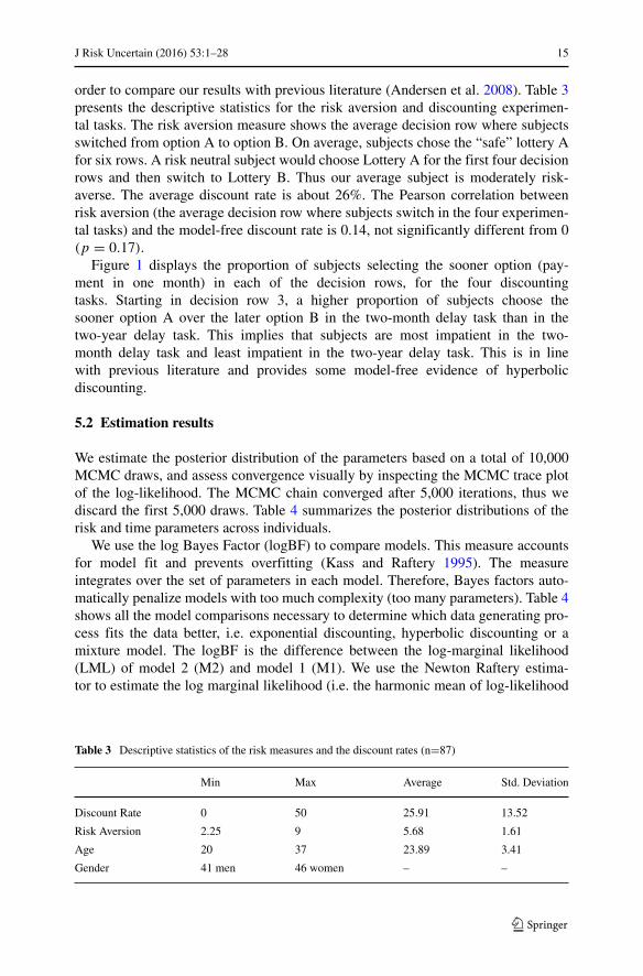
order to compare our results with previous literature (Andersen et al. 2008). Table 3presents the descriptive statistics for the risk aversion and discounting experimen-tal tasks. The risk aversion measure shows the average decision row where subjectsswitched from option A to option B. On average, subjects chose the “safe” lottery Afor six rows. A risk neutral subject would choose Lottery A for the first four decisionrows and then switch to Lottery B. Thus our average subject is moderately risk-averse. The average discount rate is about 26%. The Pearson correlation betweenrisk aversion (the average decision row where subjects switch in the four experimen-tal tasks) and the model-free discount rate is 0.14, not significantly different from 0(p = 0.17).

Figure 1 displays the proportion of subjects selecting the sooner option (pay-ment in one month) in each of the decision rows, for the four discountingtasks. Starting in decision row 3, a higher proportion of subjects choose thesooner option A over the later option B in the two-month delay task than in thetwo-year delay task. This implies that subjects are most impatient in the two-month delay task and least impatient in the two-year delay task. This is in linewith previous literature and provides some model-free evidence of hyperbolicdiscounting.

5.2 Estimation results

We estimate the posterior distribution of the parameters based on a total of 10,000MCMC draws, and assess convergence visually by inspecting the MCMC trace plotof the log-likelihood. The MCMC chain converged after 5,000 iterations, thus wediscard the first 5,000 draws. Table 4 summarizes the posterior distributions of therisk and time parameters across individuals.

We use the log Bayes Factor (logBF) to compare models. This measure accountsfor model fit and prevents overfitting (Kass and Raftery 1995). The measureintegrates over the set of parameters in each model. Therefore, Bayes factors auto-matically penalize models with too much complexity (too many parameters). Table 4shows all the model comparisons necessary to determine which data generating pro-cess fits the data better, i.e. exponential discounting, hyperbolic discounting or amixture model. The logBF is the difference between the log-marginal likelihood(LML) of model 2 (M2) and model 1 (M1). We use the Newton Raftery estima-tor to estimate the log marginal likelihood (i.e. the harmonic mean of log-likelihood

Table 3 Descriptive statistics of the risk measures and the discount rates (n=87)

Min Max Average Std. Deviation

Discount Rate 0 50 25.91 13.52

Risk Aversion 2.25 9 5.68 1.61

Age 20 37 23.89 3.41

Gender 41 men 46 women – –


draws after the burn-in period). Kass and Raftery (1995) suggest that a value oflogBF=LML of M2 - LML of M1 higher than 5 provides evidence of the superior-ity of model 2. Here, we benchmark all models against the exponential discountingmodel (M1).

5.2.1 Model comparison

The comparative results suggest that the model that best fits the data is Prelec’shyperbolic model. The value of the α parameter is significantly lower than 1 (α= 0.748, s.e. = 0.072), suggesting that participants discount more heavily rewardsreceived in the near future. Figure 2 compares the instantaneous discount rates for thehyperbolic and exponential models, assuming risk aversion and risk neutrality. Boththe exponential and Prelec’s hyperbolic model show the same basic results regard-ing elicited discount rates. Failing to correct for the curvature of the utility functionwhen eliciting time preferences results in overestimating discount rates. We use bothMazur’s hyperbolic and Prelec’s hyperbolic model to investigate a mixture specifi-cation of exponential and hyperbolic discounting. Both specifications reveal similarresults. About 60% of the subjects discount future rewards hyperbolically, while theremaining 40% discount exponentially, showing that individuals have heterogeneousunderlying discounting patterns. Given the widespread usage of exponential dis-counting and for the sake of comparison with results from earlier studies, we providea heterogeneity analysis for the exponential model in Section 5.3.

0.0

0.2

0.4

0.6

0.8

1.0

Decision row

Pro

port

ion

of s

ubje

cts

choo

sing

the

soon

er o

ptio

n

1 2 3 4 5 6 7 8 9 10

two−month delaysix−month delayone−year delaytwo−year delay

Fig. 1 Proportion of participants choosing the sooner option (option A) by decision row in the fourdiscounting tasks


5.2.2 Time preferences

Our results suggest that, on average, individuals demand relatively high interest ratesto delay consumption, and are moderately risk-averse. As depicted in Table 4, thediscount rate parameter has a posterior mean of 12.05% with the 95% credible inter-val at (9.93%, 14.49%); the average constant relative risk aversion is 0.515, with the95% credible interval at (0.418, 0.614). Assuming risk neutrality (the constant rela-tive risk aversion coefficient is set to 0), the discount rate is estimated at 22.79% witha 95% credible interval at (19.19%, 26.84%). The average discount rates after cor-recting for the curvature of the utility function are in line and strengthen the resultsfrom the literature on joint elicitation of risk and time preferences (Andersen et al.2008; Andreoni and Sprenger 2012a). Moreover, our estimated discount rates aremuch lower than what was previously reported in the intertemporal choice literature,where discount rates of the order of hundreds are not uncommon (Loewenstein andPrelec 1992; Frederick et al. 2002). Given our sample of financially educated busi-ness school students, we might expect discount rates to be lower than in other studies.Our estimated discount rates are indeed below the level reported in Andreoni andSprenger (2012a), who used a freshman and sophomore sample in their study. The

Table 4 Parameter estimates: means and standard deviations (below) of the posterior distributions (n=87)

Model Risk Noise Discount Noise Mixture logBF3

Aversion Parameter Rate Parameter Parameter

μ ν π (LML)

Exponential 0.5151a 0.041a 0.120a 0.011a −(0.05) (0.004) (0.011) (0.001) (−2,010)

Mazur’s 0.507a 0.043a 0.126a 0.009a 39

hyperbolic (0.051) (0.004) (0.012) (0.001) (−1,971)

Prelec’s 0.514a 0.041a 0.131, 0.748a 0.008a 210

hyperbolic (0.052) (0.004) (0.015, 0.072) (0.001) (−1,800)

(β, α)

Exponential/ 0.41a 0.040a 0.113 0.008 0.41062 136

Prelec’s (0.051) (0.004) (0.012) (0.001) (0.063) (−1,874)

hyperbolic 0.135, 0.651a

Mixture (0.021,0.098)

(δ, β, α)

1Statistical signif. codes:(a) 99% interval does not include 02The mixture parameter π is not statistically different than 50%3Last column reports the log-Bayes factors and log-marginal likelihoods (in brackets)The logBF is the difference between the log-marginal likelihood of the specified model minus thelog-marginal likelihood of the exponential discounting model. A value higher than 5 suggests thatthe specified model fits the data better


results are in line with Laury et al. (2012) findings, estimated with an undergradu-ate student sample from a large US university. Also, our results show slightly higherdiscount rates than reported in Andersen et al. (2008), which used a representativesample of the adult Danish population.

5.2.3 Risk preferences

Our utility curvature estimates are lower than those reported in Andersen et al.(2008) (average CRRA estimate of 0.515; s.e. = 0.050 versus 0.741; s.e. = 0.048).In turn, our results imply a higher level of risk aversion than those reported byAndreoni and Sprenger (2012a), who find that aggregate utility curvature is far closerto linear utility than estimated from the double mutiple-price list approach used inAndersen et al. (2008). Interestingly, they find no correlation between the risk esti-mates from the multiple price list approach and the convex time budget approach,despite the fact that under CRRA utility, the two elicitation methods measure thesame utility construct. This suggests that further research is necessary to assesswhich methodology is more suited to assess curvature in discounting models. Thenoise parameters, showing the extent to which subjects’ choices are due to deci-sion errors or randomness, are also within expected ranges (Holt and Laury 2002;Andersen et al. 2008). The fact that the noise parameter estimate is smaller for thetime discounting task than for the risk aversion task (0.041; s.e. = 0.004 for riskaversion versus 0.011; s.e. = 0.001 for discounting) is not surprising either, as the

0.0

0.1

0.2

0.3

0.4

0.5

0.6

Assuming risk aversion

Time horizon in years

Dis

coun

t rat

e

0 1 2

ExponentialPrelec’s hyperbolic

0.0

0.1

0.2

0.3

0.4

0.5

0.6

Assuming risk neutrality

Time horizon in years

Dis

coun

t rat

e

0 1 2

ExponentialPrelec’s hyperbolic

Fig. 2 Estimated instantaneous discount rate for hyperbolic discounters vs. exponential discounters,assuming risk aversion (left) and risk neutrality (right)


time discounting elicitation procedure is cognitively easier than the risk preferencetask.

5.3 Heterogeneity in risk and time preferences

5.3.1 Investigating possible drivers of heterogeneity—observable characteristics

The heterogeneity model presented in Section 4.3 is a special case of a hierarchicalBayes random effects model, in which the distribution of heterogeneity is recov-ered and described, but the heterogeneity in preferences is not explained by observedvariables. We extend this model and attempt to partly explain heterogeneity in riskand time preferences using the subjects’ individual differences. We collected data ongender, age, and grade in the introductory finance course if they had attended one(84/87 or 96.5% of the sample). We conduct our analysis based on the exponentialdiscounting model. Equation 11 is replaced with:

θi = �zi + ui; ui ∼ N(0, Vθ ) (11′)

where zi is a set of individual difference variables for individual i, and � capturesthe impact of covariates on subjects’ risk and time preferences. The first and second-stage priors will also reflect the changes in our model.

First-stage prior

θi ∼ N(�zi, Vθ )

Second-stage prior

vec(�|Vθ ) ∼ N(�,A−1 ⊗ Vθ)

Vθ ∼ IW(ν, V0)

Table 5 Parameter estimates for the observed heterogeneity model, showing the impact of the individualdifference variables on risk and time preferences: means and standard deviations (below) of the posteriordistributions (n=87)

Model Risk Noise Discount Noise

Parameters Aversion Parameter μ Rate Parameter ν

Intercept 0.4871a 0.049a 0.123a 0.012a

0.046 0.004 0.012 0.001

Age 0.002 −0.002 −0.065a −0.044

0.014 0.028 0.028 0.028

Gender 0.180c −0.110 −0.096 −0.448

0.098 0.180 0.177 0.186

Finance Grade −0.002 −0.031 0.035 0.065

0.021 0.03f9 0.039 0.041

1Statistical signif. codes: (a) 99% interval does not include 0. (c) 90% interval does not include 0


We estimated the model following the methodology outlined in Section 4. We mean-centered the demographic variables to be able to interpret the intercept as the averageparameters.

The explained heterogeneity model converged to a log-marginal likelihood of−2, 098. The logBF between the explained heterogeneity and the unexplained het-erogeneity model is 88. Therefore, we find strong evidence that the unexplainedheterogeneity model is more parsimonious and seems to fit the data better, as ourindividual difference variables do not seem to explain well the variance in sub-jects’ risk attitudes and intertemporal choices. In line with previous literature, wefind no significant effect of gender on intertemporal choices (Chesson and Viscusi2000). Table 5 reports two significant effects. Gender positively impacts risk aversion(λr−gender = 0.180; s.e. = 0.098). Women appear to be more risk-averse, which val-idates previous findings (Eckel and Grossman 2008; Ioannou and Sadeh 2016). Theexpected discount rate decreases with age (λδ−age = −0.065; s.e. = 0.028). Thiscontradicts previous research showing that older individuals require higher discountrates as they tend to be more concerned about receiving the payoffs within their life-time (Chesson and Viscusi 2000). Our results could be due to the limited age range inour sample. The minimum age is 20 and maximum age is 37, with a mean at 23.89.

5.3.2 Discrete heterogeneity—Cluster analysis

To explore the extent of heterogeneity in risk attitudes and intertemporal choices inthe sample, we use K-means clustering and group the decision makers in our samplebased on the individual level CRRA estimates and discount rates. After eliminatingthe outliers from this analysis (two subjects with discount rates higher than 50%), weidentify three types of decision makers, as shown in Fig. 3. Even though the screeplot does not give a clear picture with respect to the number of clusters to analyze

2 4 6 8 10

24

68

1012

Scree plot

Number of clusters

With

in g

roup

s su

m o

f squ

ares

0.0

0.1

0.2

0.3

0.4

−0.5 0.0 0.5 1.0

CRRA coefficeint

Dis

coun

t rat

e cluster

Risk Averse

Risk Neutral

Risk Seeking

Three clusters model

Fig. 3 Three-cluster model and scree plot


(either 3, 4, or 5 types are acceptable), the ease of interpretation for three groupsoutweighs the gains in variance explained (7%) from the 4-cluster model over the3-cluster model. Table 6 reports the descriptive statistics of the three groups.

Group 1 (n=14) consists of risk-seeking participants (mean CRRA is -0.10) whoare impatient and require a high discount rate (19.49% on average) to postpone con-sumption. We call this group the “low patience” type. The second group (n=28)includes moderately risk-averse subjects (mean CRRA is 0.42), who require a meaninterest rate of 16.94% to postpone consumption. This group represents individualswith average patterns of behavior on both risk and time dimensions. We label thisgroup the “moderate patience” type. The third group (n=43) embodies very risk-averse (mean CRRA is 0.79) individuals who require a low discount rate to postponeconsumption (10.75% on average). We name this group the “high patience” type.

5.3.3 Cumulative discount rate distributions

To further explore heterogeneity, we investigate the cumulative discount rate distri-bution for each level of risk decision makers are willing to accept. The cumulativediscount rate distribution refers to the percentage of participants who are willing toaccept a discount rate lower than or equal to a specific value. Given that they belongto clusters 1, 2, and 3, respectively, we know that decision makers are risk-seeking,risk neutral, and risk-averse and use this information to produce cumulative discountrate distributions for each cluster of participants.

From Fig. 4 and Table 7, we can determine that about 28% of the risk-seekingdecision makers accept a discount rate less than or equal to 15%. Sixty-four percentof the risk neutral individuals will accept a discount rate of 20% or less, while only35% of the risk-seeking individuals will accept such a discount rate. Forty-six percentof the risk-seeking people will only accept a discount rate of 25% or more, i.e. theywould reject discount rates below 25%. However, 74% of the risk neutral and 64% ofthe risk-averse decision makers will accept at least a 20% discount rate, therefore theyaccept offers between 20% and 25%, otherwise rejected by risk-seeking participants,showing that they would be more patient. Risk-seeking individuals will reject plansor policy measures that are attractive to decision makers belonging to a different type.In this context, identifying decision makers’ risk preferences and adapting to theirneeds becomes important to ensure a wide acceptance of policy measures involvingintertemporal choices.

Table 6 Cluster analysis

Groups

Low Patience Moderate Patience High Patience

CRRA −0.1 0.42 0.79

Discount Rate 19.49% 16.94% 10.75%

Group Size (%) 16% 35% 49%


0.0

0.2

0.4

0.6

0.8

1.0

Cumulative Discount Rate Distributions

Discount Rate

Per

cent

age

of p

artic

ipan

ts

0 .1 .2 .3 .4 .5 1

Risk Seeking/ Low patience typeRisk Neutral/ Moderate patience typeRisk Averse/ High patience type

Fig. 4 Cumulative distribution of discount rates for different types

5.4 Assessing the correlation between risk and time preferences

The hierarchical Bayes specification allows for a direct measure of the correlationbetween risk and time preferences, which is not possible in maximum likelihoodmethods. Table 8 reports the covariance matrix Vθ that characterizes the unexplainedvariability in risk and time preferences across subjects. The diagonal elements, show-ing posterior variances of our model parameters, are higher and show significantheterogeneity between subjects for both risk and intertemporal choices. Therefore,

Table 7 Cumulative distribution of discount rates for different types

Risk-seeking Risk-neutral Risk-averse

accept 15% or less 28.57% 53.57% 74.41%

accept 20% or less 35.71% 64.28% 95.34%

accept 25% or less 64.28% 78.57% 97.67%


there is scope for analyzing such heterogeneity via individual demographic and psy-chographic variables. The off-diagonal elements indicate similar patterns of behavioracross subjects. Although the values are based on the exponentially transformedvariables and the size of the covariance is not readily interpretable, the fact thatthe covariance is significant and negative supports the finding that more risk-averseindividuals exhibit increasing patience. The propensity for errors is lower for morerisk-averse individuals, since the covariance between the risk aversion parameter rand the noise parameters ν and μ is significant and negative. The propensity for erroris higher for more impatient individuals (cov(ν, δ)=0.425).

We use the MCMC draws to compute the parameters’ posterior means for eachsubject in our sample, based on the exponential discounting model. The correlationof these predicted values is −0.42 (p < 0.01). Therefore, we find evidence of anegative correlation between risk aversion and impatience.

We also estimate the discount rates under the assumption that subjects are riskneutral, and separately estimate individual level risk preferences. The correlationbetween discount rates under risk neutrality and CRRA coefficients is 0.16, not sig-nificant (p > 0.05). This correlation is similar in sign and size with the correlationbetween the model free discount rates and risk attitudes.

To assess whether the pattern of correlation differs between risk-seeking, risk neu-tral and risk-averse individuals, we conduct three regression analyses, each using adataset corresponding to the types reported in Section 5.2.3. We find no significantcorrelation between risk and time preferences for risk-averse and risk neutral indi-viduals (Pearson’s r = −0.219, p > 0.05, and Pearson’s r = −0.217, p > 0.05), anda significant negative correlation between risk and time preferences for risk-seekingdecision makers (Pearson’s r= −0.545, p= 0.044). This shows that the model is ableto recover various patterns of correlation in the data. Moreover, it is crucial to cor-rect for the concavity of the utility function before assessing the size and sign of thiscorrelation. We use the risk preferences task to identify the curvature of the utility

Table 8 Covariance matrix of model parameters

Risk Noise Discount Noise

Aversion r Parameter μ Rate δ Parameter ν

Risk 0.2041a −0.159a −0.112a −0.242a

Aversion r (0.032) (0.047) (0.044) (0.063)

Noise 0.560a 0.268a 0.386a

Parameter μ (0.117) (0.084) (0.120)

Discount 0.703a 0.425a

Rate δ (0.121) (0.124)

Noise 1.171a

Parameter ν (0.206)

1Statistical signif. codes:(a) 99% interval does not include 0


function. At the individual level, we obtain lower discount rates under the assumptionof risk aversion than for risk neutrality. However, this individual-level relationshipdoes not impact the correlation between risk and time preferences across subjects(Andersen et al. 2008, page 612).5

5.5 Sensitivity to background consumption

Our estimation technique requires an estimate of the background consumption ω

to control for the curvature of the utility function, as discussed in Section 4.1.We exogenously set this parameter for the above estimation at ω=12, for comparisonwith Andersen et al.’s (2008) study. To assess the sensitivity of our results to differ-ent levels of background consumption, we vary the value of ω (see Fig. 5). Andersenet al. (2008) find that their estimated discount rates are not very sensitive to thelevel of background consumption, while the CRRA coefficient increases from 0.67when ω=50 to 0.82 when ω=200. Andreoni and Sprenger (2012a) report that esti-mated discount rates double when daily consumption is varied from $3.52 to $14.09.Although their methodology to elicit curvature-controlled discount rates is invariantto the level of daily background consumption, when replicating the Andersen et al.(2008) joint estimation technique, Laury et al. (2012) find that discount rates increasefrom a low of 14.3% when ω=0 to about 20% as ω increases. We find that our esti-mates of risk and time preferences show little sensitivity to background consumption;the CRRA coefficient increases from 0.49 when ω=1 to 0.57 when ω=200. The dis-count rates increase from a low of 10.3% for ω=1 to 15.6% for ω=200, similar tothe pattern reported in Laury et al. (2012). Hence, there is a slight increase in thediscount rate when we increase background consumption.

6 Discussion and conclusions

The elicitation of risk and time preferences is pivotal in understanding individu-als’ decisions such as health-related choices (e.g., dieting, addictions), as well as indeveloping efficient public policies that impact private decisions, involving tradeoffsbetween now and the future (e.g. environmental policies, incentives for education).In this paper, we present a method to simultaneously elicit and estimate decisionmakers’ risk attitudes and intertemporal choices. We jointly elicit risk and time pref-erences, as doing so provides significantly lower discount rates than in experimentswhich assume subjects to be risk neutral, and closer to what is a priori consid-ered to be reasonable discount rates. We use a novel individual level estimationprocedure based on a hierarchical Bayes methodology, which embeds standard dis-counting functions and risk specifications from the decision making literature. The

5To check whether the negative correlation is driven by our choice of model, we conducted a simulationstudy to gauge whether we can assess different patterns of correlation. We simulate data from the model,imposing positive, negative, or no correlation between risk and time preferences. We recover all patterns ofcorrelation (simulated correlation = {0.38, −0.03, −0.38} vs. estimated correlation = {0.40, 0.09, −0.21},respectively). We thank an anonymous reviewer for raising this point.


0.0

0.1

0.2

0.3

0.4

0.5

0.6

0.7

Background consumption

1 5 12 25 50 200

Risk parameterDiscount rate

Fig. 5 Estimated discount rates and CRRA coefficients as a function of daily background consumption

method accounts for similarities among individuals and provides robust estimatesof the model parameters without ignoring the interdependency between subjects orover-weighting their individual differences. We achieve this by pulling individualestimates towards a group mean. This effect is more pronounced when estimates areless reliable, mitigating the noise in the estimation. Hierarchical Bayes modeling isparticularly useful when the number of subjects in an experiment is relatively large,while the data from each subject are few or noisy, which is the case in many deci-sion making experiments including ours. The methodology allows us to obtain moreaccurate estimates, without increasing the duration of the experiment or the numberof tasks.

Using our hierarchical Bayes methodology to jointly estimate risk and time prefer-ences, we recover the probability distributions for the group-level CRRA coefficientsand discount rates, as well as individual level risk attitudes and intertemporal choices.We find that, on average, individuals require an annual discount rate of 12% to post-pone consumption and are moderately risk-averse (the constant relative risk aversioncoefficient is 0.515). The results are in line with previous literature on risk and timepreferences and further support the need to control for the curvature of the utilityfunction when estimating discount rates in experiments. We also test the robustness ofour results against alternative specifications for time preferences, e.g. Mazur’s hyper-bolic and Prelec’s hyperbolic discounting models, as well as a mixture specification.The models are easily integrated within our joint estimation of risk and time pref-erences, another advantage of the hierarchical Bayes methodology. While Prelec’shyperbolic specification fits the data better, the qualitative results are similar to thoseimplied by exponential discounting. This implies that correcting for the curvature ofthe utility function is important in estimating discount rates.


We use the individual level parameter estimates to assess the level of heterogene-ity in risk and time preferences. We find that women tend to be more risk-averse, andpeople tend to be more patient with age. We conduct a cluster analysis and find threetypes of decision makers that vary in terms of their risk attitudes and intertempo-ral choices. Risk-averse individuals are more patient, while risk-seeking individualstend to be more impatient. This is a consequence of the reported negative correla-tion between risk attitudes and intertemporal choices. The results of the model alsosuggest that there is significant unobserved heterogeneity, worth assessing in futurestudies. Policy makers can use data on preference elicitation to offer type-specificplans or design mechanisms that produce desirable self-selection, for public policiesinvolving health issues (e.g., smoking, dieting), education requirements, or environ-mental plans. An interesting avenue for further research would be to investigate themost suitable ways to present information on public policy measures to differenttypes of decision makers.

Reassuring for environmental policy makers, Ioannou and Sadeh (2016) find thatdiscounting is similar for monetary and environmental decisions. Using an experi-mental design where subjects make choices between monetary rewards vs. plantingbee-friendly plants, the authors show that while discount rates are not statistically sig-nificantly different, people tend to be more risk-averse for environmental decisions.Ioannou and Sadeh’s (2016) study sequentially elicits risk and time preferences andreports no correlation between subjects’ discount rates and risk aversion, a result wealso confirm when eliciting risk and time preferences sequentially. Their study dif-fers from ours in a few important respects. We correct for the concavity of the utilityfunction when eliciting discount rates, and use a hierarchical Bayes methodology tosimultaneously estimate risk and time preferences. Also, Ioannou and Sadeh’s (2016)study involves real stakes, while we use hypothetical stakes. More research is nec-essary to assess the correlation between risk and time preferences across differentdomains, elicitation protocols and estimation methods.

Acknowledgments We would like to thank seminar participants at the Rotterdam School of Manage-ment, Erasmus University and the University of Texas at Dallas for helpful comments and suggestions. Weare particularly grateful to Stefano Puntoni, Jason Roos, W. Kip Viscusi, Peter Wakker, and an anonymousreferee for their insightful comments.

Open Access This article is distributed under the terms of the Creative Commons Attribution 4.0International License (http://creativecommons.org/licenses/by/4.0/), which permits unrestricted use, dis-tribution, and reproduction in any medium, provided you give appropriate credit to the original author(s)and the source, provide a link to the Creative Commons license, and indicate if changes were made.

References

Abdellaoui, M., Bleichrodt, H., l’Haridon, O., & Paraschiv, C. (2013). Is there one unifying concept ofutility? An experimental comparison of utility under risk and utility over time. Management Science,59(9), 2153–2169.

Anderhub, V., Guth, W., Gneezy, U., & Sonsino, D. (2001). On the interaction of risk and time preferences:An experimental study. German Economic Review, 2(3), 239–253.

http://creativecommons.org/licenses/by/4.0/


Andersen, S., Harrison, G.W., Lau, M.I., & Rutstrom, E.E. (2008). Eliciting risk and time preferences.Econometrica, 76(3), 583–618.

Anderson, L., & Stafford, S. (2009). Individual decision-making experiments with risk and intertemporalchoice. Journal of Risk and Uncertainty, 38(1), 51–72.

Andreoni, J., & Sprenger, C. (2012a). Estimating time preferences from convex budgets. AmericanEconomic Review, 102(7), 3333–3356.

Andreoni, J., & Sprenger, C. (2012b). Risk preferences are not time preferences. American EconomicReview, 102(7), 3357–3376.

Camerer, C. (2004). Individual decision making. In Kagel, J.H., & Roth, A.E. (Eds.), Handbook ofExperimental Economics. Princeton University Press (pp. 587–616).

Cardenas, J.C., & Carpenter, J. (2013). Risk attitudes and economic well-being in Latin America. Journalof Development Economics, 103(C), 52–61.

Chesson, H.W., & Viscusi, W.K. (2000). The heterogeneity of time-risk tradeoffs. Journal of BehavioralDecision Making, 13, 251–258.

Chesson, H.W., & Viscusi, W.K. (2003). Commonalities in time and ambiguity aversion for long-termrisks. Theory and Decision, 54, 57–71.

Coller, M., & Williams, M. (1999). Eliciting individual discount rates. Experimental Economics, 2(2),107–127.

Conte, A., Hey, J.D., & Moffatt, P.G. (2011). Mixture models of choice under risk. Journal ofEconometrics, 162, 79–88.

Eckel, C.C., & Grossman, P.J. (2008). Forecasting risk attitudes: An experimental study using actual andforecast gamble choices. Journal of Economic Behavior & Organization, 68(1), 1–17.

Falk, A., Meier, S., & Zehnder, C. (2013). Do lab experiments misrepresent social preferences? Thecase of self-selected student samples. Journal of the European Economic Association, 11(4),839–852.

Frederick, S., Loewenstein, G., & O’Donoghue, T. (2002). Time discounting and time preference: Acritical review. Journal of Economic Literature, 40(2), 351–401.

von Gaudecker, H.M., van Soest, A., & Wengstrom, E. (2011). Heterogeneity in risky choice behavior ina broad population. American Economic Review, 101(2), 664–94.

Holt, C.A., & Laury, S.K. (2002). Risk aversion and incentive effects. American Economic Review, 92(5),1644–1655.

Ioannou, C.A., & Sadeh, J. (2016). Time preferences and risk aversion: Tests on domain differences.Journal of Risk and Uncertainty, 53(1), in press.

Jackman, S. (2009). Bayesian Analysis for the Social Sciences. Wiley Series in Probability and Statistics.Wiley.

Jarnebrant, P., Toubia, O., & Johnson, E. (2009). The silver lining effect: Formal analysis and experiments.Management Science, 55(11), 1832–1841.

Kang, M.J., Rangel, A., Camus, M., & Camerer, C.F. (2011). Hypothetical and real choice differentiallyactivate common valuation areas. Journal of Neuroscience, 31(2), 461–468.

Kass, R.E., & Raftery, A.E. (1995). Bayes factors. Journal of the American Statistical Association, 90,773–795.

Kimball, M.S., Sahm, C.R., & Shapiro, M.D. (2009). Risk preferences in the psid: Individual imputationsand family covariation. Working Paper 14754, National Bureau of Economic Research.

Laibson, D. (1997). Golden eggs and hyperbolic discounting. Quarterly Journal of Economics, 112, 443–477.

Laury, S.K., McInnes, M.M., & Swarthout, J.T. (2012). Avoiding the curves: Direct elicitation of timepreferences. Journal of Risk and Uncertainty, 44(3), 181–217.

Loewenstein, G., & Prelec, D. (1992). Anomalies in intertemporal choice: Evidence and an interpretation.Quarterly Journal of Economics, 107(2), 573–597.

Mazur, J.E. (1987). An adjustment procedure for studying delayed reinforcement. In Commons, M.L.,Mazur, J.E., Nevin, J.A., & Rachlin, H. (Eds.), The Effect of Delay and Intervening Events onReinforcement Value. Erlbaum (pp. 55–76).

Meyer, A. (2013). Estimating discount factors for public and private goods and testing competingdiscounting hypotheses. Journal of Risk and Uncertainty, 46(2), 133–173.

Nilsson, H., Rieskamp, J., & Wagenmakers, E.J. (2011). Hierarchical Bayesian parameter estimation forcumulative prospect theory. Journal of Mathematical Psychology, 55(1), 84–93.


Prelec, D. (2004). Decreasing impatience: A criterion for non-stationary time preference and hyperbolicdiscounting. Scandinavian Journal of Economics, 106(3), 511–532.

Rossi, P., Allenby, G., & McCulloch, R. (2005). Bayesian Statistics and Marketing. No. 13 in Wiley seriesin probability and statistics, Wiley.

Rossi, P.E., & Allenby, G.M. (2003). Bayesian statistics and marketing. Marketing Science, 22(3), 304–328.

Taylor, M. (2013). Bias and brains: Risk aversion and cognitive ability across real and hypotheticalsettings. Journal of Risk and Uncertainty, 46(3), 299–320.

Toubia, O., Johnson, E., Evgeniou, T., & Delquie, P. (2013). Dynamic experiments for estimating pref-erences: An adaptive method of eliciting time and risk parameters. Management Science, 59(3),613–640.

heterogeneous risk and time preferences - home - … procedure based on a hierarchical bayes...

Documents