heterogeneous price setting behavior and aggregate dynamics: some general...

Heterogeneous Price Setting Behavior and Aggregate Dynamics:

Some General Results�

(PRELIMINARY; COMMENTS WELCOME)

Carlos Carvalho

Federal Reserve Bank of New York

Felipe Schwartzman

Princeton University

March 2008

Abstract

We analyze the e¤ects of heterogeneity in price setting behavior in time-dependent sticky

price and sticky information models characterized by quite general adjustment hazard functions.

In a large class of models that includes the most commonly used price setting speci�cations,

heterogeneity leads monetary shocks to have larger real e¤ects than in one-sector economies

with the same frequency of adjustments. Quantitatively, the e¤ects of heterogeneity in models

calibrated to match the recent empirical evidence on pricing behavior are large, even in the

absence of strategic complementarity in price setting. We �nd that the degree of monetary non-

neutrality in the calibrated heterogeneous economies can be as large as in an otherwise identical

one-sector economy with roughly three times more nominal rigidity.

JEL classi�cation codes: E1, E3

Keywords: heterogeneity, aggregation, price setting, general hazard function

�The views expressed in this paper are those of the authors and do not necessarily re�ect the position ofthe Federal Reserve Bank of New York or the Federal Reserve System. E-mails: [email protected],[email protected].

1

1 Introduction

We analyze the e¤ects of heterogeneity in price setting behavior in time-dependent sticky price and

sticky information models characterized by quite general adjustment hazard functions. In a large

class of models that includes the most commonly used price setting speci�cations, heterogeneity

in the frequency of price changes (in sticky price economies) and in the frequency of information

updating (in sticky information economies) leads monetary shocks to have larger real e¤ects than

in one-sector economies with the same frequency of adjustments. Quantitatively, the e¤ects of

heterogeneity in models calibrated to match the recent empirical evidence on pricing behavior are

quite large, even in the absence of strategic complementarity in price setting.

The dynamics of heterogeneous economies with such general adjustment hazard functions de-

pend on the details of the latter, and on the whole cross sectional distribution that describes how

they vary across sectors. However, for commonly used speci�cations of monetary shocks and a sen-

sible measure of monetary non-neutrality, we characterize analytically the e¤ects of heterogeneity

for arbitrary such hazard functions and cross-sectional distributions, in the absence of strategic

complementarity or substitutability - what we refer to as strategic neutrality - in price setting. Be-

sides providing analytical convenience, our focus on the case of strategic neutrality is motivated by

the challenge of producing signi�cant monetary non-neutrality with empirically plausible amounts

of nominal frictions, in the absence of the strong ampli�cation e¤ects that complementarities in

price setting are well known to generate.

Our analytical results provide conditions that determine, for a given price setting speci�cation

characterized by speci�c adjustment hazard functions, whether heterogeneity in price setting leads

to a larger or smaller extent of monetary non-neutrality than in a one-sector economy with the

same hazard function and average frequency of adjustments. We show that these conditions hold

in the most commonly used sticky price and sticky information models: the extent of monetary

non-neutrality in each sector is convex in the frequency of price adjustment/information updating.

Jensen�s inequality thus implies larger non-neutralities in the heterogeneous economies.

The intuition as to why the average frequency of adjustments can be quite misleading as an

indicator of the overall degree of nominal frictions can be developed from the following limiting

case: a two-sector sticky price continuous time economy with a non-negligible fraction of �rms that

adjust prices continuously, i.e., a �exible price sector. Then, irrespective of how low the frequency

of price adjustments in the other sector is, the average frequency in the economy will be in�nite.

Nevertheless, monetary shocks may still have large real e¤ects due to the sticky price sector.

The intuition of our extreme example carries through to the general case, and does not depend

on continuous time. While in one-sector economies there is a direct relationship between the average

frequency of price changes (information updating) and the average duration of price spells (spells

2

between information updating), this is not the case in heterogeneous economies: a given average

frequency of adjustments is consistent with very di¤erent distributions for the average duration

of spells between adjustments across sectors. As a result, in heterogeneous economies, contrary

to one-sector economies, a high average frequency of adjustment need not imply small monetary

non-neutralities.

We explore the quantitative e¤ects of heterogeneity in calibrated versions of two well established

models: a sticky price model with Taylor (1979) staggered price setting, and the sticky information

model of Mankiw and Reis (2002). Under strategic neutrality in price setting, we �nd that the

degree of monetary non-neutrality in the calibrated heterogeneous economies can be as large as

in an otherwise identical one-sector economy with roughly three times more nominal rigidity. We

analyze the role of complementarities and its interaction with heterogeneity in the calibrated models.

In line with the results of Carvalho (2006), who analyzes heterogeneity in price stickiness in the

Calvo (1983) model, and Carvalho (2008), who analyzes heterogeneity in two sticky information

models, we �nd that strategic complementarities in price setting amplify the role of heterogeneity

in generating larger monetary non-neutrality, by leading sectors that are slower to adjust prices (or

update information) to have a disproportionate impact on the aggregate price level.

As a by-product of our analytical results, we uncover the features of the distribution of the

duration of price spells (spells between information updating) that determine the extent of mon-

etary non-neutrality for di¤erent types of shocks. For empirically plausible shocks, we �nd that

the �rst three moments of such distribution su¢ ce to characterize the extent of monetary non-

neutrality, according to our measure. Thus, future empirical work on price setting should attempt

to document these other moments of the distribution of the duration of price spells. We also un-

cover the somewhat surprising result that the extent of monetary non-neutrality measured as the

discounted cumulative real e¤ects of monetary surprises is the same in sticky price and sticky infor-

mation economies that share the same adjustment hazard functions (as well as all other structural

features).1 It turns out to be a direct implication of optimal price setting and rational expectations.

Our case for studying heterogeneity in sticky price models builds directly on the empirical

evidence. Recently, a series of important papers have documented several features of price setting

behavior in both the U.S. economy and the Euro area using disaggregated price data that underlies

consumer price indices (Bils and Klenow 2004, for the U.S. economy; Dhyne et al. 2006, and

references cited therein for the Euro area). In particular, such papers uncover a vast amount of

heterogeneity in the frequency of price changes across di¤erent sectors of these economies. As for

sticky information, there is hardly any direct evidence on the frequency with which �rms update

their information in order to set prices. However, there is no a priori reason why �rms in di¤erent

1Of course the hazard functions play di¤erent roles in sticky price and sticky inforamtion economies. In theformer they decribe the impediments to continuous price adjustment, whereas in the latter they describe the frictionsthat prevent continuous information updating.

3

sectors should behave similarly in this dimension. In fact, sticky information models are best seen

as a reduced form of a microfounded model in which �rms face explicit costs to acquire and process

information, and optimally choose for how long to wait before updating their information again

(Reis, 2006). Therefore, we should actually expect �rms in di¤erent sectors to update information

at di¤erent frequencies, because the optimal time period in-between such �updating dates�depends

on factors such as the magnitude of those costs, the importance of sectoral shocks to demand and

marginal costs and the shape of the pro�t function, which are all likely to vary across sectors.

A substantial body of research addresses issues that are related to the subjects of this paper.

Following Bils and Klenow (2004), there is now a large empirical literature that documents hetero-

geneity in price setting behavior using micro-data that underlies price indices (Dhyne et al. 2006

list many references for the Euro area, and there are also similar papers for numerous other coun-

tries). Bils and Klenow (2002, 2004), Bils et al. (2003) and Ohanian et al. (1995) are examples

of papers that allow for heterogeneity in price stickiness in the context of time-dependent mod-

els. In earlier work, Taylor (1993) extended his original model (1979, 1980) to account for wage

contracts of di¤erent durations. In a di¤erent framework, with state- rather than time-dependent

pricing rules, Caballero and Engel (1991, 1993) also allow for heterogeneity in the frequency of price

changes. These papers do not focus, however, on isolating the role of heterogeneity in aggregate

dynamics. This latter kind of analysis is undertaken by Aoki (2001) and Benigno (2001, 2004),

who explore the e¤ects of heterogeneity in price stickiness on optimal monetary policy in two-sector

models.2 Nakamura and Steinsson (2007a) perform such an analysis in a state-dependent pricing

model. Dixon and Kara (2005) study the role of heterogeneity in a model with Taylor staggered

wage setting. Carlstrom et al. (2006) use a two-sector model with di¤erent degrees of nominal

rigidity to study how sectoral relative prices a¤ect aggregate dynamics. Barsky et al. (2007) study

a two-sector model with durable consumption goods and heterogeneity in the frequency of price

changes. Sheedy (2007a) studies how heterogeneity in price stickiness a¤ects in�ation persistence.

Imbs et al. (2007) study the aggregation of sectoral Phillips curves, and the statistical biases that

can arise from not accounting for heterogeneity. Finally, Carvalho and Nechio (2008) show that an

open economy model with heterogeneity in price stickiness can account for the sluggish dynamics

of real exchange rates observed in the data, whereas a one-sector version of the model with the

same average degree of price stickiness fails to do so.

The use of more general adjustment hazard functions in sticky price models is common to some

recent papers. Wolman 1999, Mash 2004, Guerrieri 2006, Coenen et al. 2007, and Sheedy 2007b

allow for �exible adjustment hazard functions in time-dependent models. Caballero and Engel

(2007) study generalized (S,s) pricing models in which the adjustment hazard function is somewhat

general. They argue that for empirically relevant parameterizations of such function, the degree

2Benigno (2001) extends some of his results to a multi-region setting.

4

of aggregate price �exibility implied by the generalized (S,s) model is roughly three times as large

as the frequency of price adjustments. None of these papers, however, considers the e¤ects of

heterogeneity in pricing behavior.

To our knowledge ours is the �rst paper to incorporate heterogeneity in price setting into

sticky price and sticky information models with general adjustment hazard functions. Our results

show that in a large class of sticky price and sticky information models that includes the ones

most commonly used in the literature, heterogeneity in pricing behavior is a powerful source of

ampli�cation of monetary shocks, even in the absence of pricing complementarities. They con�rm

the recent �ndings of Carvalho (2006, 2008), whose results on heterogeneity in price setting are a

particular case of our sticky price and sticky information models. Together with recent results by

Nakamura and Steinsson (2007a) on the e¤ects of heterogeneity in a calibrated menu-cost model, our

work suggests that one-sector models have a strong tendency to understate the extent of monetary

non-neutrality, irrespective of the nature of frictions that prevent continuous and fully informed

reassessment of pricing decisions.

The rest of the paper is organized as follows. Section 2 presents the basic setup and introduces

the two price setting models in separate subsections. Section 3 presents a general equivalence result

between sticky price and sticky information models built on the basis of the same adjustment hazard

functions. Section 4 presents the main analytical results for our measure of monetary non-neutrality.

Section 5 analyzes the implications of sectoral heterogeneity for monetary non-neutrality in the most

commonly used models of price setting, and provides conditions under which the results can be

generalized to other models. Section 6 presents quantitative results in calibrated sticky price and

sticky information models. The last section concludes.

2 Model

We start with the description of the economic environment that would obtain in the absence of

any impediments to continuous price adjustments and updating of information - what we refer to

as the frictionless environment. Such impediments, which characterize the sticky price and sticky

information models, are introduced subsequently.

2.1 Frictionless economy

A representative consumer derives utility from a Dixit-Stiglitz composite of di¤erentiated consump-

tion goods and supplies a continuum of di¤erentiated types of labor to monopolistically competitive

�rms, which he owns. The latter are divided into sectors, and indexed by their sector, k 2 K, andby j 2 [0; 1]. The distribution of �rms across sectors is summarized by a density function f on K

5

(with cdf F ).3 Each �rm hires labor of a speci�c type in a competitive market to produce a likewise

speci�c variety of the consumption good. We assume a cashless economy with a risk-free nominal

bond in zero net supply.

The representative consumer maximizes:

Z 1

0e��t

C (t)1�� 11� � �

Zk2K

f (k)

Z 1

0

Lkj (t)1+ 1

'

1 + 1'

djdk

!dt

s:t: _B (t) = i (t)B (t) +

Zk2K

f (k)

Z 1

0Lkj (t)Wkj (t) djdk � P (t)C (t) + T (t) ; for t � 0;

and a no-Ponzi condition. Here � is the discount rate, C (t) is consumption of the composite good,

Lkj (t) is the supplied quantity of type kj labor, Wkj (t) is the associated nominal wage, T (t) are

�rms��ow pro�ts received by the consumer, B (t) denotes bond holdings that accrue interest at

rate i (t), and P (t) is a price index to be de�ned below. The parameters ��1 and ' stand for the

intertemporal elasticity of substitution in consumption and the (Frisch) elasticity of labor supply,

respectively.

The composite consumption good is given by:

C (t) ��Zk2K

f (k)��1Ck (t)

��1� dk

� ��1

; (1)

Ck (t) � f (k)

�Z 1

0Ckj (t)

"�1" dj

� ""�1

; (2)

where Ck (t) is the subcomposite of goods produced by �rms in sector k, and Ckj (t) is consumption

of the variety of the good produced by �rm j from sector k (henceforth ��rm kj�).4 The elasticity

of substitution between varieties within a sector is " > 1, and � > 0 is the elasticity of substitution

across di¤erent sectors. Denoting by Pkj (t) the price charged by �rm kj at time t, the corresponding

consumption price index is:

P (t) =

�Zk2K

f (k)Pk (t)1�� dk

� 11��

;

Pk (t) =

�Z 1

0Pkj (t)

1�" dj

� 11�"

;

3 In the frictionless environment described in this subsection prices are fully �exible and �rms have full informationabout the state of the economy at all times. As a result, there are no di¤erences between such sectors, and the notationis introduced here for convenience. In subsequent subsections we introduce sector-speci�c adjustment hazard functionsindexed by k, which describe price setting behavior in di¤erent sectors. In addition, in this frictionless environmentnominal shocks have no real e¤ects, and so we delay the introduction of uncertainty to later sections.

4The normalization in the sectoral aggregators yields a symmetric equilibrium in which when �rms choose thesame prices they sell the same quantities. In this case the di¤erences in total output across sectors only depends onthe measure of �rms in each sector.

6

where Pk (t) is a sectoral price index.

The �rst order conditions for the representative consumer�s optimization problem are:

Wkj (t)

P (t)=Lkj (t)

1'

C (t)��; kj 2 K � [0; 1] ;

_C (t)

C (t)= ��1

"��

i (t)�

_P (t)

P (t)

!#;

Ck (t) = f (k)C (t)

�Pk (t)

P (t)

��; k 2 K;

Ckj (t) = f (k)�1Ck (t)

�Pkj (t)

Pk (t)

��"; kj 2 K � [0; 1] ;

In this frictionless environment, �rms solve a simple, static pro�t maximization problem. Firm

kj hires labor of its speci�c type in a competitive labor market to produce its variety of the

consumption good according to a linear technology:

Ykj (t) = Nkj (t) ;

where Ykj (t) is the production of its variety and Nkj (t) is the speci�c labor input.5 The �rm�s

problem is then given by:

maxP �kj(t)

�P �kj (t)Ykj (t)�Wkj (t)Nkj (t)

�s:t: Ykj (t) = Nkj (t) ;

Ykj (t) =

P �kj (t)

Pk (t)

!�"�Pk (t)

P (t)

��Y (t) ;

where

Y (t) ��Zk2K

f (k)��1Yk (t)

��1� dk

� ��1

;

Yk (t) � f (k)

�Z 1

0Ykj (t)

"�1" dj

� ""�1

;

and where we have used the market clearing conditions in the goods markets. The optimal fric-

5As in the more standard identical-�rms model, the assumption of speci�c input markets is perfectly compatiblewith price-taking behavior. For a detailed discussion of this point see Woodford (2003, ch. 3).

7

tionless price is given by the usual mark-up rule:

P �kj (t) ="

"� 1Wkj (t) :

The model is closed by a monetary policy speci�cation that ensures existence and uniqueness

of a rational expectations equilibrium.

2.2 Price setting in the presence of frictions

We obtain our sticky price and sticky information models from the above frictionless environment

by introducing frictions to price setting. Impediments to continuous price adjustment yield the

sticky price models, whereas infrequent information updating gives rise to the sticky information

models. Heterogeneity arises because the extent of such frictions is allowed to vary across sectors.

In the frictionless environment of the previous section monetary shocks are immaterial, and thus

were omitted for simplicity. This is no longer the case in the presence of frictions, and from now

on we account for uncertainty stemming from monetary shocks.

Frictions to price setting are characterized by sector-speci�c �survival� functions e�k (t; t+ s).The latter have di¤erent interpretations in the two types of models that we consider: in the sticky

price models e�k (t; t+ s) denotes the probability that a price set at time t by a �rm in sector k will

still be in place at time t + s (and possibly thereafter); in sticky information models, e�k (t; t+ s)gives the probability that a �rm from sector k that updates its information set - and therefore its

price plan - at time t will still be using the same price plan at time t+ s (and possibly thereafter).6

At this stage, the only restriction we impose on e�k is that lims!1 e�k (t; t+ s) = 0, which rules outno-adjustment (no-updating) on the part of �rms. We emphasize that such survival functions are

sector-speci�c in the sense that in each sector all �rms follow the pricing policies that they imply,

and not in the sense that all �rms in each sector change prices (update information) at the same

time.

2.2.1 Sticky prices

In the presence of the aforementioned impediments to continuous price adjustments, when setting

its price Xspkj (t) at time t �rm kj solves:

max Et

Z 1

0Qsp (t; t+ s) e�k (t; t+ s) hXsp

kj (t)Yspkj (t+ s)�W

spkj (t+ s)N

spkj (t+ s)

ids

6Without loss of generality we assume that e�k (t; t+ s) is de�ned for s 2 [0;1). Models in which the duration ofprice spells (or of price plans) is �nite with probability one are naturally included.

8

s:t: Y spkj (t+ s) = Nspkj (t+ s) ;

Y spkj (t+ s) =

Xspkj (t)

P spk (t+ s)

!�"�P spk (t+ s)

P sp (t+ s)

��Y sp (t+ s) ;

where the �sp�superscript stands for sticky price, and the nominal discount factor between t and

t+ s used to price �rms�pro�ts, Qsp (t; t+ s), is given by:7

Qsp (t; t+ s) = e��sP sp (t)

P sp (t+ s):

The �rst order condition yields:

Xspkj (t) =

"

"� 1EtR1t Qsp (t; s) e�k (t; s)P spk (s)"�� P sp (s)� Y sp (s)W sp

kj (s) ds

EtR1t Qsp (t; s) e�k (t; s)P spk (s)"�� P sp (s)� Y sp (s) ds

:

We focus on the symmetric equilibrium in which, conditional on time t information, the joint

distribution of future variables that matter for price setting is the same for all �rms in sector k that

change prices in period t, and therefore they choose the same nominal price. Thus, the sectoral

price indices are given by:

P spk (t) =

�Z t

�1�k (s) e�k (s; t)Xsp

k (s)1�" ds

� 11�"

; (3)

where �k (s) denotes the fraction of �rms from sector k that change prices at s.

Given an arbitrary heterogeneous sticky price economy characterized bynf; e�k;�ko

k2K, let

its corresponding sticky information economy be the sticky information economy characterized by

the same primitives, including the functionsnf; e�k;�ko

k2K, where the interpretation of e�k is, of

course, di¤erent. We derive and aggregate �rms� optimal pricing policies in the corresponding

sticky information economy in the next subsection. For notational convenience, henceforth we use

fSkgk2K to denote thenf; e�k;�ko

k2Kstructure.

2.2.2 Sticky information

In line with the sticky information model proposed by Mankiw and Reis (2002), �rms only update

their information sets sporadically. There are no impediments to price adjustment, so that �rms set

prices at each instant to maximize current expected pro�ts, conditional on their current (possibly

outdated) information. At time t a �rm kj that last updated its information set at time t � s7Alternatively, under complete markets the nominal stochastic discount factor would take on the usual form

Qsp (t; t+ s) = e��s�Csp(t+s)Csp(t)

��Psp(t)

Psp(t+s). This di¤erence is immaterial in the log-linear approximate model ana-

lyzed subsequently.

9

solves:8

maxXsikj(t�s;t)

Et�s

"�Xsikj (t� s; t)�W si

kj (t)� Xsi

kj (t� s; t)P sik (t)

!�"�P sik (t)

P si (t)

��Y si (t)

#;

where the �si�superscript stands for sticky information. Thus, it sets:

Xsikj (t� s; t) =

"

"� 1Et�s

hP sik (t)

"�� P si (t)� Y si (t)W sikj (t)

iEt�s

�P sik (t)

"�� P si (t)� Y si (t)� :

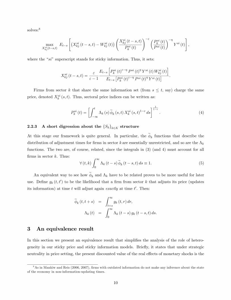
Firms from sector k that share the same information set (from s � t, say) charge the same

price, denoted Xsik (s; t). Thus, sectoral price indices can be written as:

P sik (t) =

�Z t

�1�k (s) e�k (s; t)Xsi

k (s; t)1�" ds

� 11�"

: (4)

2.2.3 A short digression about the fSkgk2K structure

At this stage our framework is quite general. In particular, the e�k functions that describe thedistribution of adjustment times for �rms in sector k are essentially unrestricted, and so are the �k

functions. The two are, of course, related, since the integrals in (3) (and 4) must account for all

�rms in sector k. Thus:

8 (t; k)Z 1

0�k (t� s) e�k (t� s; t) ds � 1: (5)

An equivalent way to see how e�k and �k have to be related proves to be more useful for lateruse. De�ne gk (t; t0) to be the likelihood that a �rm from sector k that adjusts its price (updates

its information) at time t will adjust again exactly at time t0. Then:

e�k (t; t+ s) =

Z 1

t+sgk (t; r) dr;

�k (t) =

Z 1

0�k (t� s) gk (t� s; t) ds:

3 An equivalence result

In this section we present an equivalence result that simpli�es the analysis of the role of hetero-

geneity in our sticky price and sticky information models. Brie�y, it states that under strategic

neutrality in price setting, the present discounted value of the real e¤ects of monetary shocks is the

8As in Mankiw and Reis (2006, 2007), �rms with outdated information do not make any inference about the stateof the economy in non-information-updating times.

10

same in sticky price and sticky information economies that share the same fSkgk2K structure.

In general, the dynamics of the heterogeneous economies encompassed by our framework depend

on the whole cross sectional distribution of the functions e�k and �k, and analytical results aredi¢ cult to obtain. To make the problem more tractable, we work with log-linear approximate

versions of the models, and with a sensible scalar measure of monetary non-neutrality for which we

can derive analytical results. We also assume that monetary shocks take the form of innovations

to an exogenous nominal aggregate demand process.9

We start by presenting log-linear versions of the price setting models, approximated around a

(common) deterministic zero in�ation steady state. Then we present our equivalence result.

3.1 Log-linear sticky price models

Firms from sector k that change prices at t set:10

xspk (t) =

R1t e��(s�t)e�k (t; s)Et h1+'�1�1+'�1"p

sp (s) + '�1("��)1+'�1" p

spk (s) +

'�1+�1+'�1"y

sp (s)idsR1

t e��(s�t)e�k (t; s) ds :

When '�1("��)1+'�1" = 0, � � '�1+�

1+'�1" corresponds to the Ball and Romer (1990) index of real

rigidities. In that case, prices are strategic complements (substitutes) if � < 1 (> 1). The dividing

case implies neither complementarity nor substitutability, and we refer to it as neutrality in price

setting. It arises, for instance, under logarithmic utility and linear disutility of labor.

The aggregate price level is given by:

psp (t) =

Zk2K

f (k) pspk (t) dk;

where the sectoral price indices evolve according to:

pspk (t) =

Z t

�1�k (s) e�k (s; t)xspk (s) ds:

9This is a common speci�cation in the literature, usually justi�ed by the assumption that the monetary authoritysets its policy instrument so as to generate the postulated nominal aggregate demand process. Despite the lack ofrealism as a description of monetary policy, the assumption of shocks to an exogenous nominal aggregate demandprocess usually leads to useful insights. Carvalho (2006) shows that the conclusions about the role of heterogeneity inprice stickiness in the Calvo model obtained with such assumption continue to hold when monetary policy is modeledin an empirically more realistic fashion.

10From now on lowercase variables denote log-deviations from the deterministic zero in�ation symmetric steadystate.

11

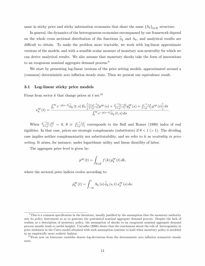
3.2 Log-linear sticky information models

Firms from sector k that last updated information at t� s set:

xsik (t� s; t) = Et�s�1 + '�1�

1 + '�1"psi (t) +

'�1 ("� �)1 + '�1"

psik (t) +'�1 + �

1 + '�1"ysi (t)

�:


psi (t) =

Zk2K

f (k) psik (t) dk;

with sectoral price indices evolving according to:

psik (t) =

Z t

�1�k (s) e�k (s; t)xsik (s; t) ds:

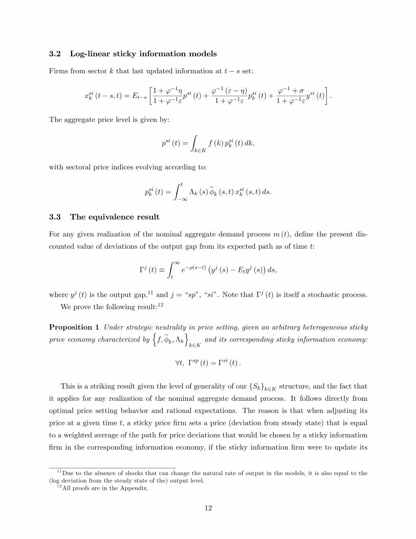
3.3 The equivalence result

For any given realization of the nominal aggregate demand process m (t), de�ne the present dis-

counted value of deviations of the output gap from its expected path as of time t:

�j (t) �Z 1

te��(s�t)

�yj (s)� Etyj (s)

�ds;

where yj (t) is the output gap,11 and j = �sp�, �si�. Note that �j (t) is itself a stochastic process.

We prove the following result:12

Proposition 1 Under strategic neutrality in price setting, given an arbitrary heterogeneous sticky

price economy characterized bynf; e�k;�ko

k2Kand its corresponding sticky information economy:

8t; �sp (t) = �si (t) :

This is a striking result given the level of generality of our fSkgk2K structure, and the fact thatit applies for any realization of the nominal aggregate demand process. It follows directly from

optimal price setting behavior and rational expectations. The reason is that when adjusting its

price at a given time t, a sticky price �rm sets a price (deviation from steady state) that is equal

to a weighted average of the path for price deviations that would be chosen by a sticky information

�rm in the corresponding information economy, if the sticky information �rm were to update its

11Due to the absence of shocks that can change the natural rate of output in the models, it is also equal to the(log deviation from the steady state of the) output level.

12All proofs are in the Appendix.

12

information set at the same given time t. The weights are given by the discount factor and by the

likelihood that the price will still be in e¤ect until the various dates.

Proposition 1 should not be taken to imply that the dynamic responses of a heterogeneous

sticky price economy and of its corresponding sticky information economy to monetary shocks are

the same. In fact, we know that in general they di¤er. Nevertheless, this result turns out to

be extremely useful. The reason is that it implies that the extent of monetary non-neutrality in

sticky price and sticky information economies that share the same fSkgk2K structure is the same,

according to the scalar measure of non-neutrality that we use to study the e¤ects of heterogeneity

in price setting. This allows us to focus on just one class of models, and to obtain sharp analytical

results, to which we turn next.

4 Measuring the extent of monetary non-neutrality

The result of the previous section is quite general. However, it does not allow us to quantify the

extent of monetary non-neutrality. In particular, the fact that the fSkgk2K structure potentially

varies over time makes the problem non-stationary, in the sense that the dates on which the shocks

hit matter through the distribution of price adjustment and price plan revision times implied by

fSkgk2K .To arrive at a useful measure of the extent of monetary non-neutrality we impose restrictions

on fSkgk2K . to obtain stationarity. This allows us to derive a general expression for our measureof monetary non-neutrality. We then specialize to two types of monetary shocks for which we can

derive sharp analytical results: shocks to the level of nominal aggregate demand (�level shocks�),

and shocks to the growth rate of nominal aggregate demand (�growth rate shocks�).

We use these results in Section (5) to analyze the e¤ects of heterogeneity on the extent of

monetary non-neutrality in the most commonly used sticky price and sticky information models.

We also provide general conditions under which heterogeneity in price setting behavior increases

the extent of monetary non-neutrality.

4.1 Restrictions on e�k and �k, and auxiliary resultsFrom the de�nition of the e�k;�k and gk functions:

e�k �t; t0� =

Z 1

t0gk (t; s) ds;

�k (t) =

Z 1

0�k (t� s) gk (t� s; t) ds:

13

For e�k to be stationary (i.e., to depend only on t0� t; not on t) we need gk (t; s) to depend only ons� t. In that case, we can write: e�k (�) = Z 1

�gk (s) ds;

where now e�k (�) denotes the probability that a price (price plan) of a �rm from sector kwill last

for an interval of length � or more. Accordingly, gk (s) denotes the likelihood that such a price

(price plan) will last exactly for an interval of length s.

In addition, for the extent of monetary non-neutrality to be independent of the date on which

the shock hits, we also need �k (t) to be time-invariant: 8t; �k (t) � �k. This amounts to requiringthat the measure of �rms adjusting prices (updating information) at any given point in time be

constant, and corresponds to the assumption of uniform staggering, common in this class of models.

It follows from (5) that:

8k;Z 1

0�ke�k (�) d� = 1;

so that �k =�R10e�k (�) d��1.

We can now de�ne, for each sector, �k (�) � �ke�k (�), and prove the following results:Lemma 1 At any given time t, �k (�) gives the density of �rms in sector k that will adjust prices

(revise price plans) again exactly at t+ � .

As a result of Lemma 1, we shall refer to �k (�) as the density associated with the distribution

of remaining durations of prices (price plans) already in place at any given point in time.

Lemma 2 Let �k � Egk [� ] �R10 gk (�) �d� denote the expected duration of price spells (price

plans) for newly set prices (price plans) in sector k. Then:

�k =1

�k:

As a result of Lemma 2, we shall refer to �k as the average frequency of price changes (infor-

mation updating) in sector k.

Note that in general the expected duration of price spells (price plans) for newly set prices

(price plans) by �rms in sector k; �k, di¤ers from the expected remaining duration of prices (price

plans) already in place at any point in time in that sector, E�k [� ] �R10 �k (�) �d� . However, if the

time elapsed since the price (price plan) was set does not a¤ect the distribution of the time interval

until the next adjustment (plan revision), then the two expected durations should be equal. This

is exactly the case for models with constant adjustment hazards. The adjustment hazard function

gives the likelihood of adjustment (information updating) taking place at a given point in time in

the life of the price spell (price plan), conditional on it not having taken place until then. In terms

14

of our notation, the adjustment hazard function for sector k is given by:

hk (�) =gk (�)

1�Gk (�);

where:

Gk (�) =

Z �

0gk (s) ds:

The irrelevance of the time elapsed since the last price adjustment (price plan revision) in

constant hazard models is formalized in the following:

Lemma 3 For models with constant adjustment hazards:

gk (�) = �k (�) :

Finally, in the following sections we derive results that relate the extent of monetary non-

neutrality to moments of the distributions that characterize price setting behavior in our economies.

Thus, from now on we assume the technical condition 8k; lim�!1��3 (1�Gk (�))

�= 0, which

guarantees that the relevant moments exist.

4.2 A measure of monetary non-neutrality

A one-time monetary shock hits the economy at time zero, yielding thereafter a (perfect foresight)

path for nominal aggregate demand denoted by m� (t).13 Prior to the shock the latter is assumed

to have been evolving according to m (t). We measure the degree of monetary non-neutrality by the

discounted cumulative e¤ect of the shock on the output gap. More speci�cally, our measure of non-

neutrality is given by � =R10 e��syj (s) ds, which from Proposition 1 is the same in sticky price

and sticky information economies that share the same ff; �k;�kgk2K structure, under strategic

neutrality in price setting. For ease of exposition, from now on we assume those conditions and

focus on heterogeneous sticky information economies.

The price level in our heterogeneous sticky information economy at a time t � 0 is given by:

p(t) =

Zk2K

�Z 0

�1�k (t� s)m (t) ds+

Z t

0�k (t� s)m� (t) ds

�dF (k) : (6)

13 In looking at the perfect foresight response to a one-time shock we make use of the fact that certainty equivalenceholds in our (loglinear) sticky price and sticky information models.

15

Using (6), our measure of monetary non-neutrality becomes:

� =

Z 1

0e��t [m� (t)� p (t)] dt (7)

=

Zk2K

�Z 1

0e��t [m� (t)�m (t)] [1� �k (t)] dt

�dF (k) ;

where �k (t) =R t0 �k(s)ds = 1 �

R1t �k(s)ds. Given the restrictions imposed in the previous

subsection, our measure of non-neutrality amounts to the average discounted surprises in nominal

aggregate demand weighted by the total fraction of �rms at each point in time which last updated

their information sets before the shock hit.

4.3 Level shocks to nominal aggregate demand

A shock to the level of nominal aggregate demand that dies out exponentially at rate can be

modeled as:

m�(t)�m(t) =

8<: 0; t < 0

e� t; t � 0;

where without loss of generality the size of the shock has been normalized to unity.

In this context, we prove the following:

Proposition 2 For a small discount rate (�! 0) ; the expected discounted cumulative e¤ect on

the output gap of a persistent shock ( ! 0) to the level of nominal aggregate demand equals the

economy-wide expected remaining duration of price plans put in place before the shock hit:

lim�; !0 � =

Zk2K

E�k [� ]dF (k) ;

where, as de�ned previously, E�k [� ] �R10 �k (�) �dt.

Proposition 2 relates the extent of monetary non-neutrality with a moment of the economy-

wide distribution of times until the next price plan revisions, f�kgk2K . As explained in subsection(4.1), that distribution refers to price plans that were in place when the shock hit, and in general

di¤ers from the distribution of durations of newly set price plans. Our next result relates the extent

of non-neutrality directly to moments of the cross-sectional distribution of durations of newly set

price plans.

Proposition 3 For a small discount rate (�! 0) ; the expected discounted cumulative e¤ect on the

16

output gap of a persistent shock ( ! 0) to the level of nominal aggregate demand is given by:

lim�; !0 � =1

2

Zk2K

�2k + �2k

�kdF (k) ;

where as de�ned previously �k � Egk [� ] �R10 gk (�) �dt is the expected duration of a newly set

price plan by a �rm in sector k, and �2k � V argk [� ] �R10 gk (�) (� � �k)2 d� is the variance of the

duration of such a plan.

4.4 Growth rate shocks to nominal aggregate demand

A shock to the growth rate of nominal aggregate demand that dies out exponentially at rate � can

be modeled as:

m�(t)�m(t) =

8<: 0; t < 0

1�e��t� ; t � 0;

where without loss of generality the size of the shock has been normalized to unity.

In this context, we prove the following:


the output gap of a persistent shock (�! 0) to the growth rate of nominal aggregate demand equals

(half) the cross-sectional average of the second moment of the distribution of remaining durations

of price plans put in place before the shock hit:

lim�;�!0 � =1

2

Zk2K

E�k [�2]dF (k) ;

where E�k [�2] �

R10 �k(�)�

2d� .

In analogy with Proposition 3, our next result relates the extent of non-neutrality generated

by growth rate shocks directly with moments of the cross-sectional distribution of durations of

newly set price plans (prices).

Proposition 5 For a small discount rate (�! 0) ; the expected discounted cumulative e¤ect on the

output gap of a persistent shock (�! 0) to the growth rate of nominal aggregate demand equals

lim�;�!0 � =1

6

Zk2K

�2k + 3�2k +

Skewgk [� ]

�kdF (k) ;

where Skewgk [� ] =R10 gk (�) (� � �k)3 d� is the skewness of the distribution of the duration of a

newly set price plan (price) by a �rm in sector k.

17

5 The e¤ects of sectoral heterogeneity

In this section we assess the implications of heterogeneity in price setting for the extent of monetary

non-neutrality. To isolate the role of heterogeneity, we make comparisons with otherwise identical

one-sector economies with the same average frequency of price changes (information updating) as

the heterogeneous economy. We start by looking at the most commonly used sticky price and sticky

information speci�cations, and then draw lessons for a wider class of models.

5.1 Constant hazard models

The most common sticky price models - built on the Calvo (1983) model - and the seminal sticky

information model of Mankiw and Reis (2002) assume constant adjustment hazards. In that context

the distribution of duration of price spells (price plans) in sector k is given by:

gk (�) = �ke��k� :

By de�nition, �k = ��1k , and direct calculations yield:

�2k = �2k;

Skewgk [� ] = 2�3k:

The e¤ects of persistent level and growth rate shocks to nominal aggregate demand are, respec-

tively:

Level: lim�; !0 � =1

2

Zk2K

�2k + �2k

�kdF (k) =

Zk2K

�kdF (k) ;

Growth rate: lim�;�!0 � =1

6

Zk2K

�2k + 3�2k +

Skewgk [� ]

�kdF (k) =

Zk2K

�2kdF (k) :

An otherwise identical one-sector economy with the same average frequency of price changes

(information updating) has constant adjustment hazard equal to � =Rk2K �kdF (k), with implied

duration of price rigidity equal to ��1. Thus, because �k = ��1k , Jensen�s inequality directly implies

that both for persistent level and growth rate shocks to nominal aggregate demand, the extent of

monetary non-neutrality is larger in heterogeneous economies:

Level:Zk2K

�kdF (k) =

Zk2K

��1k dF (k) >

�Zk2K

�kdF (k)

��1= ��1;

Growth rate:Zk2K

�2kdF (k) =

Zk2K

��2k dF (k) >

�Zk2K

�kdF (k)

��2= ��2:

18

This simply re�ects the fact that what matters for the extent of non-neutrality is the distribution

of times until prices (price plans) are adjusted after the shock hits. To further sharpen the intuition

as to why the average frequency of adjustments can be quite misleading as an indicator of the overall

degree of nominal frictions, consider the following limiting case: a two-sector sticky price economy

with a non-negligible fraction of �rms that adjust prices continuously, i.e., a �exible price sector.

Then, irrespective of how low the frequency of price adjustments in the other sector is, the average

frequency in the economy will be in�nite. Nevertheless, monetary shocks may still have large real

e¤ects due to the sticky price sector.

The intuition of our extreme example carries through to the general case. While in one-sector

economies there is a direct relationship between the average frequency of price changes (infor-

mation updating) and the average duration of spells between adjustments, this is not the case in

heterogeneous economies: a given average frequency of adjustments is consistent with very di¤erent

distributions for the average duration of spells between adjustments across sectors. As a result, in

heterogeneous economies, contrary to one-sector economies, a high average frequency of adjustment

need not imply small monetary non-neutralities.

5.2 Constant duration models

The sticky price models inspired by the seminal work of Taylor (1979) assume that the duration

of price spells is constant. In turn, Dupor and Tsuruga (2005) analyze a sticky information model

with constant time intervals between information updatings. In those cases the distribution of

duration of price spells (price plans) is degenerate: every newly set price (price plan) by �rms in

sector k lasts �k with probability one.14 Thus, for constant duration models, �2k = Skewgk [� ] = 0.

The e¤ects of persistent level and growth rate shocks to nominal aggregate demand in those

models are, respectively:

Level: lim�; !0 � =1

2

Zk2K

�2k + �2k

�kdF (k) =

Zk2K

1

2�kdF (k) ;

Growth rate: lim�;�!0 � =1

6

Zk2K

�2k + 3�2k +

Skewgk [� ]

�kdF (k) =

Zk2K

1

6�2kdF (k) :

An otherwise identical one-sector economy with the same average frequency of price changes

(information updating) has a duration of price rigidity equal to ��1, where � =Rk2K �kdF (k).

Thus, arguments analogous to those in the previous subsection imply that both for persistent level

and growth rate shocks to nominal aggregate demand, the extent of monetary non-neutrality is

larger in heterogeneous economies.

14Formally, in this case there is no underlying density gk (�), and the problem should be written with the Diracmeasure.

19

5.3 Other models

The two previous subsections show that in the most common sticky price and sticky information

models, heterogeneity in price setting increases the extent of monetary non-neutrality. Beyond

that, however, the generality of our framework comes at the cost of making it hard to make precise

statements about models with adjustment hazard functions that are essentially unrestricted. To il-

lustrate the di¢ culty, consider a two-sector sticky price economy in which one sector features Calvo,

and the other Taylor pricing (yes, the generality of our framework allows for that). One can obvi-

ously compute moments of the distribution of the frequency of price changes in the heterogeneous

economy, but how should one construct a one-sector economy with which to make comparisons?

While potentially an interesting research question, it is beyond the scope of this paper. We avoid

these complications by restricting the nature of heterogeneity so that the adjustment hazard func-

tions in all sectors come from a single parametric family with a �nite number of parameters, which

in turn are allowed to di¤er across sectors.

Our previous analytical results suggest that for the types of shocks that we analyze, the �rst

three moments of the distribution of duration of price spells (spells between information updatings)

su¢ ce to determine the extent of monetary non-neutrality.15 Thus, it seems natural to restrict

attention to three-parameter parametric families for the adjustment hazard functions. However,

the empirical literature on price setting does not provide us with enough detailed information

to go beyond the frequency of price changes.16 As a result, we illustrate one application of the

analytical results in our general framework with a one-parameter family. To make the narrative

simpler we describe the idea for a sticky price economy. In that case the one-sector economy with

the same average frequency of price changes is clearly de�ned given the parametric adjustment

hazard, and the �rst three moments of the distribution of durations of price spells implied by

the hazard can be written as a function of the frequency of price changes. A simple test for

whether heterogeneity implies larger or smaller non-neutralities in an economy characterized by

that adjustment hazard function amounts to verifying whether the �moments�17 �2k+�2k

�k(for level

shocks) and �2k+3�2k+

Skewgk [� ]

�k(for growth rate shocks) are convex or concave in the frequency of

price changes. The concept underlying our simple test generalizes to the case of a parametric family

with more parameters. In that case, the additional degrees of freedom combined with additional

moments are used to �nd the parameters for the one-sector economy. After that, one can assess

how cross-sectional heterogeneity a¤ects the resulting expression for the extent of monetary non-

neutrality.

15We say suggest, because our results are based on limiting cases for the shocks.16To make justice to their contribution, Nakamura and Steinsson (2007b) provide a lot more information on price

setting behavior beyond the frequency of price changes. However, there is no information about the moments thatwe uncover with our analytical results.

17 In this case these are simply functions of the frequency of price changes.

20

It is clear that even within the class of three-parameter families, there is literally an in�nite

number of models in which heterogeneity implies larger non-neutralities. At the same time, there

is an in�nite number of cases in which it does not. To take some natural examples, consider

parametric families in which the variance and skewness of the distribution of duration of price

spells are constant, i.e. do not depend on the frequency of price changes. Then, heterogeneity

unequivocally implies larger non-neutralities in response to level shocks.18 For growth rate shocks,

this is also the case for all positively skewed distributions, and for negatively skewed ones as well,

as long as jSkewgk [� ]j � �3k: For strongly negatively skewed distributions (Skewgk [� ] � ��3k), thisis no longer the case.

6 Quantitative results

In this section we address the quantitative importance of the results highlighted previously. As a

result of our choice of a scalar measure of non-neutrality and of our simplifying assumptions on

preferences, we temporarily left aside the issues of how heterogeneity a¤ects the shape of impulse

response functions in sticky price and sticky information models, and of whether there are any

interactions between strategic complementarities and heterogeneity in price setting. We now address

these issues as well.

We use calibrated versions of a heterogeneous sticky price model with Taylor staggered price

setting and of a heterogeneous sticky information economy based on Mankiw and Reis (2002). We

compare those models with identical �rms economies with the same average frequency of informa-

tion updating and price changes, respectively.

We choose to calibrate the cross sectional distribution of adjustment frequencies based on data

on prices analyzed by Bils and Klenow (2004). We group the di¤erent categories of goods and

services reported in their paper into a number of representative frequencies of price changes, and

then map each such frequency into a sector in the models. This is arguably a sensible interpretation

of their data in the context of a sticky price model. However, sticky information models are at odds

with such micro evidence on nominal price rigidity, since they imply continuous price adjustment.

Moreover, there is hardly any direct evidence on the frequency with which �rms update their

information in order to set prices. In the absence of a better alternative we use the same set of

statistics to calibrate the cross sectional distribution of frequencies of information updating in the

Mankiw-Reis model.19 Each model is brie�y developed in a separate subsection below.

The mapping from the Bils and Klenow data to the parameters of the model is done in a way

18Just note that in that case �2k+�2k

�kis convex in �k:

19Arguably, one advantage of using such data over an arbitrary distribution is that the frequency of price changesis likely to be at least weakly related to the frequency with which �rms gather and process information that is relevantfor their pricing decisions.

21

that is consistent with continuous time models, as in Carvalho (2006).20 Their sample contains 350

goods and services categories. The average frequency of price changes implies that prices change

on average every 2:9 months. The median frequency of price changes implies that a newly set price

lasts on average for 4:3 months. Finally, the expected duration of a newly set price implied by

the distribution of frequencies of price changes equals 6:6 months. The cross-sectional standard

deviation of expected durations of newly set prices is 7:1 months. Bils and Klenow (2004) base

their analysis on adjustment frequencies rather than on directly observed spells of price rigidity in

order to avoid having to deal with censored observations. For that reason, we assume that their

statistics relate to the distribution of newly set prices, and thus we use them to calibrate gk (rather

than �k).

6.1 A �rst pass on the e¤ects of heterogeneity

As a �rst pass on the implications of heterogeneity in price setting behavior for the extent of mon-

etary non-neutrality, we use the analytical results derived in the previous section. For the limiting

cases of shocks to nominal aggregate demand, we can use the moments derived from the statistics

in Bils and Klenow to compare the extent of monetary non-neutrality in a heterogeneous economy

endowed with such a cross-sectional distribution for the frequency of price changes (information

updating), and the extent of non-neutrality in an otherwise identical one-sector economy with the

same average frequency of price changes (information updating).

For very persistent shocks to the level of nominal aggregate demand, the ratio of our measure

of the extent of monetary non-neutrality in the heterogeneous economy to the same measure in the

one-sector economy exceeds two: it equals 6:6 months2:9 months � 2:3. For very persistent shocks to the growthrate of nominal aggregate demand, the analogous ratio is much larger: it equals 6:6

2+7:12

2:92� 11:2.

The �rst pass quantitative e¤ects are quite large. For example, if we are to use a one-sector

economy to match the extent of non-neutralities generated by level shocks to nominal aggregate

demand in a heterogeneous economy, we need to calibrate the one-sector economy with less than

half of the average frequency of price adjustments observed in the data. For persistent growth rate

shocks we would need to calibrate the one-sector economy to feature on average one adjustment

everyp6:62 + 7:12 = 9:69 months rather than once every 2:9 months as in the data.

One can argue that these results are only indicative of the e¤ects of heterogeneity in these

models, for at least a couple of reasons. First, they refer to our scalar measure of monetary non-

neutrality, which by de�nition ignores the multi-dimensional features of impulse-response functions.

Second, they only hold exactly for the limiting cases for nominal aggregate demand shocks, and

with the restrictions on primitives that rule out complementarity or substitutability in price setting

decisions. In the next subsections we address these issues in calibrated models.

20 It is detailed in the Appendix.

22

6.2 Sticky information

We adopt a constant adjustment hazard function speci�cation, which is the continuous time ana-

logue of that used by Mankiw and Reis (2002): �rms only update their information sets when they

receive a �Poisson signal.�The hazard rate for �rms in sector k is �k, so that the expected duration

of price plans for �rms in this sector is �k = ��1k .

There are no impediments to price adjustment, so that �rms set prices at each instant to

maximize current expected pro�ts, conditional on their current (possibly outdated) information.

Firms from sector k that last updated information at t� s set:

xk (t� s; t) = Et�s�1 + '�1�

1 + '�1"p (t) +

'�1 ("� �)1 + '�1"

pk (t) +'�1 + �

1 + '�1"y (t)

�:


p (t) =

Zk2K

f (k) pk (t) dk;

with sectoral price indices evolving according to:

pk (t) = �k

Z t

�1e��k(t�s)xk (s; t) ds:

Our calibration assumes � = 1, ' = 0:25, � = 0, and " = � = 8. This yields an index of real

rigidities � = 0:15, which implies that pricing decisions are strategic complements.21 Figures 1 (a-

f) display the impulse response functions (IRF) of the calibrated heterogeneous sticky information

economy and its identical �rms counterpart to di¤erent shocks. All cases include IRFs both with

and without strategic complementarities in price setting.

From these results it is clear that heterogeneity ampli�es the extent of monetary non-neutralities

in a substantial way. It is also clear that strategic complementarities interact with heterogeneity to

generate more persistent real e¤ects of monetary shocks. Complementarities do make the adjust-

ment process more sluggish in the identical �rms case. With heterogeneity, however, this is even

more so, according to several metrics: the recession troughs are delayed, output is lower than in

the identical �rms economy essentially during the whole process, and takes much longer to return

to the steady state; in�ation is, accordingly, also more persistent.

21Woodford (2003, ch. 3) argues that values in the 0.10-0.15 range can be obtained with plausible assumptionsfor various sources of real rigidities.

23

6.3 Taylor staggered price setting

Building on Taylor (1979, 1980), in this model �rms are assumed to set prices for a �xed period of

time. Firms from sector k set prices for a period of length �k. Adjustments are uniformly staggered

across time in terms of both �rms and sectors. When setting prices at time t, �rms from sector k

choose:

xk (t) =�

1� e��k

Z �k

0e��sEt

�1 + '�1�

1 + '�1"p (t+ s) +

'�1 ("� �)1 + '�1"

pk (t+ s) +'�1 + �

1 + '�1"y (t+ s)

�ds:

The aggregate price level is then given by:

p (t) =

Zk2K

f (k) pk (t) dk;

with

p(t) =1

�k

Z �k

0xn(t� s)ds:

The calibration for �, ', �, "; and � is the same as in the previous subsection. To solve this

model with strategic complementarities, we discretize it and apply standard solution methods for

discrete time linear rational expectations models. For computational reasons, we solve the model

with 25 sectors. The calibration from the Bils and Klenow (2004) data is adjusted accordingly, as

detailed in the Appendix. Figures 2 (a-d) display the impulse response functions of the calibrated

heterogeneous economy and its one-sector counterpart to growth rate shocks with di¤erent levels of

persistence. Again, we contrast cases with and without strategic complementarities in price setting.

The one-sector economy is a standard Taylor staggered price setting economy with a contract length

of 3 months.

From these results it is again clear that heterogeneity in this model ampli�es the extent of

monetary non-neutralities in a substantial way. As before, strategic complementarities interact

with heterogeneity to generate more persistent real e¤ects of monetary shocks. Complementarities

do make the adjustment process more sluggish in the identical �rms case, but even more so when

there is heterogeneity.

7 Conclusion

This paper shows that the e¤ects of heterogeneity in price setting behavior documented in the

context of a sticky price model with Calvo pricing by Carvalho (2006), and two sticky information

models by Carvalho (2008) carry over to a much larger class of sticky price and sticky information

models. Moreover, in calibrated versions of a sticky information model based on Mankiw and Reis

24

(2002), and a sticky price model with Taylor staggered price setting, we �nd the quantitative e¤ects

of heterogeneity to be large. Our results suggest that heterogeneity in price setting behavior has

important aggregate implications, irrespective of the nature of frictions that prevent continuous,

fully informed price adjustments.

25

Appendix

Proofs of lemmas and propositions

Proposition 1 Let �j (t) �R1t e��(r�t)

�yj (r)� Etyj (r)

�dr; with j = �sp�, �si�. Under

strategic neutrality in price setting, given an arbitrary heterogeneous sticky price economy charac-

terized bynf; e�k;�ko

k2Kand its corresponding sticky information economy:

8t; �sp (t) = �si (t) :

Proof. De�ne �� (t) � �si (t)� �sp (t). Then:

�� (t) =

Z 1

te��(r�t)

�ysi (r)� Etysi (r)

�dr �

Z 1

te��(r�t) (ysp (r)� Etysp (r)) dr

=

Z 1

te��(r�t)

�m (r)� psi (r)� Et

�m (r)� psi (r)

��dr

�Z 1

te��(r�t) (m (r)� psp (r)� Et (m (r)� psp (r))) dr

=

Z 1

te��(r�t)

��psi (r) + Etpsi (r)

�dr �

Z 1

te��(r�t) (�psp (r) + Etpsp (r)) dr

=

Z 1

te��(r�t)

��psp (r)� psi (r)

�� Et

�psp (r)� psi (r)

��dr:

Recall that

psp (t) =

Zk2K

f (k)

Z 1

0�k (t� s) e�k (t� s; t)xspk (t� s) dsdk;

psi (t) =

Zk2K

f (k)

Z 1

0�k (t� s) e�k (t� s; t)xsik (t� s; t) dsdk;

with

xspk (t) =

R10 e��se�k (t; t+ s)Et [psp (t+ s) + �ysp (t+ s)] dsR1

0 e��se�k (t; t+ s) ds ;

xsik (t� s; t) = Et�s�psi (t) + �ysi (t)

�:

26

So, �� (t) =

Z 1

te��(r�t)

Zk2K

0@ R10 �k (r � s) e�k (r � s; r) �xspk (r � s)� xsik (r � s; r)� ds

�EtR10 �k (r � s) e�k (r � s; r) �xspk (r � s)� xsik (r � s; r)� ds

1A dF (k) dr

=

Z 1

te��(r�t)

Zk2K

0BBBBBB@

R r�t0 �k (r � s) e�k (r � s; r) �xspk (r � s)� xsik (r � s; r)� ds

+R1r�t �k (r � s) e�k (r � s; r) �xspk (r � s)� xsik (r � s; r)� ds

�EtR r�t0 �k (r � s) e�k (r � s; r) �xspk (r � s)� xsik (r � s; r)� ds

�EtR1r�t �k (r � s) e�k (r � s; r) �xspk (r � s)� xsik (r � s; r)� ds

1CCCCCCA dF (k) dr

For s � r � t, xspk (r � s) = Etxspk (r � s), and xsik (r � s; r) = Etxsik (r � s; r), so that:

Z 1

te��(r�t)

Zk2K

0@ R1r�t �k (r � s) e�k (r � s; r) �xspk (r � s)� xsik (r � s; r)� ds

�EtR1r�t �k (r � s) e�k (r � s; r) �xspk (r � s)� xsik (r � s; r)� ds

1A dF (k) dr = 0:Thus,

�� (t) =

Z 1

0e��r

Zk2K

26664R r0 �k (t+ r � s) e�k (t+ r � s; t+ r)

f�xspk (t+ r � s)� xsik (t+ r � s; t+ r)

��Et

�xspk (t+ r � s)� xsik (t+ r � s; t+ r)

�gds

37775 dF (k) dr:

To rewrite the expression above in a convenient way, perform the following change of variables:

r = z + w; s = w, with z and w ranging from 0 to 1. This yields:

�� (t) =

Z 1

0e��z

Zk2K

�k (t+ z)

26664R10 e��we�k (t+ z; t+ z + w)

f�xspk (t+ z)� xsik (t+ z; t+ z + w)

��Et

�xspk (t+ z)� xsik (t+ z; t+ z + w)

�gdw

37775 dF (k) dz:

Under strategic neutrality in price setting, � = 1. As a result, the price setting equations that

determine xspk and xsik simplify to:

xspk (t) =

R10 e��we�k (t; t+ w)Et [m (t+ w)] dwR1

0 e��we�k (t; t+ w) dw ;

xsik (t; t+ w) = Etm (t+ w) :

27

Combining the two equations, optimal price setting implies:Z 1

0e��we�k (t; t+ w) �xspk (t)� xsik (t; t+ w)� dw = 0;

Finally, for all z � 0 the Law of Iterated Expectations implies:Z 1

0e��we�k (t+ z; t+ z + w)Et �xspk (t+ z)� xsik (t+ z; t+ z + w)� dw = 0:

So,

�� (t) = 0:

Lemma 1 At any given time t, �k (�) gives the density of �rms in sector k that will adjust

prices (revise price plans) again exactly at t+ � .

Proof. We use our stationarity assumptions, and �x t = 0 without loss of generality. The

fraction of prices (price plans) in sector k set before time 0 that will be readjusted (revised) after

� is given by: Z 1

�

Z 1

s=0�kgk (s+ t) dsdt:

Let �k (�) be the fraction of prices (price plans) in sector k set before time 0 that will be readjusted

(revised) at or before � ; i.e.:

�k (�) = 1�Z 1

�

Z 1

s=0�kgk (s+ t) dsdt:

This is the same as:

�k (�) = 1�Z 1

0�k

Z 1

�gk (s+ t) dtds

= 1�Z 1

0�k~�k (s+ �) ds

= 1�Z 1

0�k (s+ �) ds

= 1�Z 1

��k (s) ds:

The fact that �k =�R10e�k (�) d��1 implies R10 �k (s) ds = 1, and as a result:

�k (�) =

Z �

0�k (s) ds:

28

Therefore, �k (�) is the corresponding density.

Lemma 2 Let �k � Egk [� ] �R10 gk (�) �d� denote the expected duration of price plans (price

spells) for newly set price plans (prices) in sector k. Then:

�k =1

�k:

Proof. Recall that: e�k (�) = �k (�)

�k=

Z 1

�gk (s) ds:

So,

�k (�) = �k

Z 1

�gk (s) ds

= �k (1�Gk (�)) ;

where

Gk (�) =

Z �

0gk (s) ds:

The fact thatR10 �k (s) ds = 1 implies

R10 �k (1�Gk (s)) ds = 1. Integrating by parts yields:

�kEgk [� ] = 1:

Lemma 3 For models with constant adjustment hazards:

gk (�) = �k (�) :

Proof. Multiplying both sides of the above expression by �k (1�Gk (�)) and using the de�ni-tion of the adjustment hazard function yields:

hk (�) �k (1�Gk (�)) = �kgk (�) :

Now, recall that �k (1�Gk (�)) = �k (�) ; so that:

hk (�)�k (�) = �kgk (�) :

29

With constant adjustment hazards - hk (�) = hk; say - the fact that both �k (�) and gk (�) are

densities, and therefore integrate to unity, implies hk = �k. As a result,

gk (t) = �k (t) :


the output gap of a persistent shock ( ! 0) to the level of nominal aggregate demand equals the

economy-wide expected remaining duration of price plans put in place before the shock hit:

lim�; !0 � =

Zk2K

E�k [� ]dF (k) ;

where, as de�ned previously, E�k [� ] �R10 �k (�) �dt.

Proof.

� =

Z 1

0e��t (m� (t)� p (t)) dt =

Zk2K

�Z 1

0e�(�+ )t [1� �k (t)] dt

�dF (k) :

To calculate the inner integral, integrate by parts:

Z 1

0e�(�+ )t [1� �k (t)] dt =

"� (1� �k (t))

e�(�+ )t

�+

#1t=0

�Z 1

0

e�(�+ )t

�+ �k(t)dt:

Note that �k(0) = 0; �k(1) = 1. So,Z 1

0e�(�+ )t [1� �k (t)] dt =

1

�+

�1�

Z 1

0e�(�+ )t�k(t)dt

�:

Now, note thatR10 e�(�+ )��k(�)d� = E�k

�e�(�+ )�

�=M�k (� (�+ )) is the Moment Generating

Function associated with the density �k(�). So, the inner integral is:Z 1

0e�(�+ )��k(�)d� =

1

�+

�1�M�k (� (�+ ))

�:

As �; ! 0, both the numerator and the denominator of the above expression go to zero. We can

�nd the limit using l�Hopital�s rule:

lim�; !0

Z 1

0e�(�+ )��k(�)d� = �M0

�k(0) =

Z 1

0��k(�)d� = E�k [� ]:

30

As a result, our measure of non-neutrality is:

lim�; !0 � =

Zk2K

E�k [� ]dF (k) :


the output gap of a persistent shock ( ! 0) to the level of nominal aggregate demand is given by:

lim�; !0 � =1

2

Zk2K

�2k + �2k

�kdF (k) ;

where as de�ned previously �k � Egk [� ] �R10 gk (�) �dt is the expected duration of a newly set

price plan by a �rm in sector k, and �2k � V argk [� ] �R10 gk (�) (� � �k)2 d� is the variance of the

duration of such a plan.

Proof. From Proposition 2:

lim�; !0 � =

Zk2K

E�k [� ]dF (k) =

Zk2K

Z 1

0��k(�)d�dF (k) :

Recall that �k (�) = �k (1�Gk (�)), and so our measure of non-neutrality can be written as:Zk2K

�k

�Z 1

0� (1�Gk (�)) d�

�dF (k) :

Integrating by parts yields:

lim�; !0 � =1

2

Zk2K

�2k + �2k

�kdF (k) :



(half) the cross-sectional average of the second moment of the distribution of remaining durations

of price plans put in place before the shock hit:

lim�;�!0 � =1

2

Zk2K

E�k [�2]dF (k) ;

where E�k [�2] �

R10 �k(�)�

2d� .

31

Proof.

� =

Z 1

0e��t (m� (t)� p (t)) dt =

Zk2K

Z 1

0

e��t � e�(�+�)t�

[1� �k (t)] dt!dF (k) :

To calculate the inner integral, integrate by parts:

1

�

�Z 1

0e��t [1� �k (t)] dt�

Z 1

0e�(�+�)t [1� �k (t)] dt

�=

1

�

�� (1� �k (t))

e��t

�

�1t=0

�Z 1

0

e��t

��k(t)dt

�� 1�

"� (1� �k (t))

e(�+�)t

�+ �

#1t=0

�Z 1

0

e�(�+�)t

�+ ��k(t)dt

!:

Note that �k(0) = 0; �k(1) = 1. So, the above expression simpli�es to:

1

�

"�1

��Z 1

0

e��t

��k(t)dt

��

1

�+ ��Z 1

0

e�(�+�)t

�+ ��k(t)dt

!#:

Using the Moment Generating FunctionM�k , the previous expression can be written as:

1

��

�1�M�k (��)

�� 1

� (�+ �)

�1�M�k (� (�+ �))

�=

(�+ �)

�� (�+ �)

�1�M�k (��)

��

�� (�+ �)

�1�M�k (� (�+ �))

�=

��+ �� (�+ �)M�k (��)

�� M�k (� (�+ �))

�� (�+ �)

:

As �! 0, both the numerator and the denominator in the above expression go to zero. So, we can

�nd the limit using l�Hopital�s rule:

lim�!0

��+ �� (�+ �)M�k (��)

�� M�k (� (�+ �))

�� (�+ �)

=1�M�k (��)� �M

0�k(��)

�2:

Next, using l�Hopital�s rule once more to take the limit of the above expression as �! 0, yields:

lim�!0

1�M�k (��)� �M0�k(��)

�2=1

2M00

�k(0) =

1

2

Z 1

0�2�k(�)dt =

1

2E�k [�

2]:

32

The order in which the limits are taken does not matter in this case, and as a result our measure

of non-neutrality is equal to:

lim�;�!0 � =1

2

Zk2K

E�k [�2]dF (k) :



lim�;�!0 � =1

6

Zk2K

�2k + 3�2k +

Skewgk [� ]

�kdF (k) ;

where Skewgk [� ] =R10 gk (�) (� � �k)3 d� is the skewness of the distribution of the duration of a

newly set price plan (price) by a �rm in sector k.

Proof. From Proposition 4:

lim�;�!0 � =1

2

Zk2K

E�k [�2]dF (k) =

1

2

Zk2K

Z 1

0�k(�)�

2d�dF (k) :

Recall that �k (�) = �k (1�Gk (�)), and thus our measure of non-neutrality can be written as:

lim�;�!0 � =

Zk2K

�k2

�Z 1

0�2 (1�Gk (�)) d�

�dF (k) :

Integrating by parts and recalling that ��1k = �k yields:

lim�;�!0 � =1

6

Zk2K

�2k + 3�2k +

Skewgk [� ]

�kdF (k) ;

where Skewgk [� ] =R10 gk (�) (� � �k)3 d� .

Cross sectional distribution based on Bils and Klenow (2004)

We group the di¤erent categories of goods and services listed in the appendix in Bils and

Klenow (2004) into a number of representative frequencies of price changes, and then map each

such frequency into a sector in the models. Recall that we use the data to calibrate frequencies of

information updating in the sticky information model as well, although the data refers to frequencies

of price changes.

33

For the sticky information model, we simply group all items that display the same monthly

frequency of adjustment. This results in 142 sectors.22 We take �k, the monthly frequency of

adjustment reported for the categories identi�ed with sector k, and compute the expected duration

of price plans according to �k = �1ln(1��k) . The underlying rate of arrival of information updating

dates in the continuous time constant hazard model is then such that �k = 1 � e��k . That is,�k = � ln (1� �k) = ��1k . Finally, we set each sectoral weight equal to the sum of the CPI weights

for the categories that have that given frequency of price changes, and renormalize so that sectoral

weights add up to one. This approach yields the sample statistics presented in Table 1.

Table 1: Moments of the Distribution of the Frequency of Price ChangesDescription Formula Months

�Inverse average frequency�duration of price ridigity

��1

; � =P142k=1 f (k) �k 2:9

�Median frequency based�du-ration of price ridigity�

��1med =�1

ln(1��med) 4:3

Average duration of pricerigidity��

� =P142k=1 f (k) �k; �k = �

�1k 6:6

Standard deviation of dura-tions of price rigidity��

�P142k=1 f (k) (�k � �)

2�1=2

7:1

Obs: Based on the statistics reported by Bils and Klenow (2004). ��med denotes the weighted medianfrequency of price changes in their data. �Technically, �k is the expected duration of price spells insector k. So, this is actually the cross-sectional average of the expected durations of price spells.��Thisis the cross-sectional standard deviation of the expected sectoral durations of price spells.

For the Taylor pricing model our approach is slightly di¤erent, because with complementarities

the model has to be solved numerically, and the state space grows fast in the number of sectors

(quadratically). As a result, solving the model with as many sectors becomes infeasible. To

circumvent this problem we construct the distribution of contract lengths from the BK data in

a slightly di¤erent way. We discretize the model to apply standard methods for solving discrete

time linear rational expectations models, taking a time period to be one month. We consider

contract lengths which are multiples of one month, and aggregate the goods and services categories

so that the ones which have an expected duration of price spells (�k as computed above) between

zero and one month (inclusive) are assigned to the one month contract length sector; the ones

with an expected duration of price spells between one (exclusive) and two months (inclusive) are

assigned to the two month contract length sector, and so on. The sectoral weights are aggregated

22The dynamics of this economy is identical to that of the economy calibrated directly with the original 350categories analyzed by Bils and Klenow (2004). This grouping by common frequencies simply makes computationsmore e¢ cient.

34

accordingly. We proceed in this fashion until the sector with contract lengths of 24 months. Finally,

we aggregate all the remaining categories, which have mean durations of price rigidity between 24

and 80 months, into a sector with 25-month contracts.23 This gives rise to 25 sectors with an

�inverse average frequency duration of price rigidity�of 3:45 months, an average contract length of

6:7 months, and a standard deviation of contracts of 5:6 months.

23The total weight of these categories is approximately 2%.

35

References

[1] Aoki, K. (2001), �Optimal Monetary Policy Responses to Relative-Price Changes,�Journal of

Monetary Economics 48: 55-80.

[2] Ball, L. and D. Romer (1990), �Real Rigidities and the Non-Neutrality of Money,�Review of

Economic Studies 57: 183-203.

[3] Barsky, R., C. House and M. Kimball (2007), �Sticky Price Models and Durable Goods,�

American Economic Review 97: 984-998.

[4] Benigno, P. (2001), �Optimal Monetary Policy in a Currency Area,�CEPR Working Paper

No. 2755.

[5] (2004), �Optimal Monetary Policy in a Currency Area,�Journal of Interna-

tional Economics 63: 293-320.

[6] Bils, M. and P. Klenow (2002), �Some Evidence on the Importance of Sticky Prices,�NBER

Working Paper #9069.

[7] (2004), �Some Evidence on the Importance of Sticky Prices,�Journal of Po-

litical Economy 112: 947-985.

[8] Bils, M., P. Klenow and O. Kryvtsov (2003), �Sticky Prices and Monetary Policy Shocks,�

Federal Reserve Bank of Minneapolis Quarterly Review 27: 2-9.

[9] Blinder, A., E. Canetti, D. Lebow and J. Rudd (1998), Asking about Prices: A New Approach

to Understanding Price Stickiness, Russell Sage Foundation.

[10] Caballero, R. and E. Engel (1991), �Dynamic (S, s) Economies,�Econometrica 59: 1659-1686.

[11] (1993), �Heterogeneity and Output Fluctuations in a Dynamic Menu-Cost

Economy,�Review of Economic Studies 60: 95-119.

[12] (2007), �Price Stickiness in Ss Models: New Interpretations of Old Results,�

Journal of Monetary Economics 54: 100-121.

[13] Calvo, G. (1983), �Staggered Prices in a Utility Maximizing Framework,�Journal of Monetary

Economics 12: 383-98.

[14] Carlstrom, C., T. Fuerst, F. Ghironi and K. Hernandez (2006), �Rel-

ative Price Dynamics and the Aggregate Economy,� mimeo available at

http://copland.udel.edu/~kolver/research/index.html.

36

[15] Carvalho, C. (2006), �Heterogeneity in Price Stickiness and the Real E¤ects of Monetary

Shocks,�Frontiers of Macroeconomics: Vol. 2 : Iss. 1, Article 1.

[16] (2008), �Sticky Information Economies with Heterogeneity in Price Setting,�

unpublished mimeo.

[17] Carvalho, C. and F. Nechio (2008), �Aggregation and the PPP Puzzle in a Sticky Price Model,�

unpublished mimeo.

[18] Coenen, G., A. Levin, and K. Christo¤el (2007), �Identifying the In�uences of Nominal and

Real Rigidities in Aggregate Price-Setting Behavior,� Journal of Monetary Economics 54:

2439-2466.

[19] Dhyne, E., L. Álvarez, H. Le Bihan, G. Veronese, D. Dias, J. Ho¤man, N. Jonker, P. Lünne-

mann, F. Rumler and J. Vilmunen (2006), �Price Changes in the Euro Area and the United

States: Some Facts from Individual Consumer Price Data,�Journal of Economic Perspectives

20: 171-192.

[20] Dixon, H. and E. Kara (2005), �Persistence and Nominal Inertia in a Generalized Taylor

Economy: How Longer Contracts Dominate Shorter Contracts,�ECB Working Paper Series

no. 489.

[21] Dupor, B. and T. Tsuruga (2005), �Sticky Information: The Impact of Di¤erent Information

Updating Assumptions,�Journal of Money, Credit and Banking 37: 1143:1152.

[22] Guerrieri, L. (2006), �The In�ation Persistence of Staggered Contracts,� Journal of Money,

Credit and Banking 38: 483:494.

[23] Haltiwanger, J. and M. Waldman (1991), �Responders Versus Non-Responders: A New Per-

spective on Heterogeneity,�Economic Journal 101: 1085-1102.

[24] Imbs, J., Jondeau, E., and F. Pelgrin (2007), �Aggregating Phillips Curves,�ECB Working

Paper Series no. 785.

[25] Mankiw, G. and R. Reis (2002), �Sticky Information Versus Sticky Prices: A Proposal to

Replace the New Keynesian Phillips Curve,�Quarterly Journal of Economics 117: 1295-1328.

[26] (2006), �Pervasive Stickiness,�American Economic Review, Papers and Pro-

ceedings, 96: 164-169.

[27] (2007), �Sticky Information in General Equilibrium,�Journal of the European

Economic Association 5: 603-613.

37

[28] Mash, Richard (2004), �Optimising Microfoundations for In�ation Persistence,�University of

Oxford Economics Series Working Papers #183.

[29] Nakamura, E. and J. Steinsson (2007a), �Monetary Non-Neutrality in a Multi-Sector Menu

Cost Model,�mimeo available at http://www.columbia.edu/~js3204/cu-papers.html.

[30] (2007b), �Five Facts About Prices: A Reevaluation of Menu Cost Models,�

mimeo available at http://www.columbia.edu/~en2198/papers.html.

[31] Ohanian, L., A. Stockman and L. Kilian (1995), �The E¤ects of Real and Monetary Shocks in

a Business Cycle Model with Some Sticky Prices,�Journal of Money, Credit and Banking 27:

1209-1234.

[32] Reis, R. (2006), �Inattentive Producers,�Review of Economic Studies 73: 793-821.

[33] Sheedy, K. (2007a), �In�ation Persistence When Price Stickiness Di¤ers Between Industries,�

mimeo available at http://personal.lse.ac.uk/sheedy/.

[34] (2007b), �Intrinsic In�ation Persistence,� mimeo available at

http://personal.lse.ac.uk/sheedy/.

[35] Taylor, J. (1979), �Staggered Wage Setting in a Macro Model,�American Economic Review

69: 108-113.

[36] (1980), �Aggregate Dynamics and Staggered Contracts,�Journal of Political

Economy 88: 1-23.

[37] (1993),Macroeconomic Policy in a World Economy: From Econometric Design

to Practical Operation, W. W. Norton.

[38] Wolman, A. (1999), �Sticky Prices, Marginal Cost, and the Behavior of In�ation,� Federal

Reserve Bank of Richmond Economic Quarterly 85 (Fall 1999), 29-48.

[39] Woodford, M. (2003), Interest and Prices: Foundations of a Theory of Monetary Policy,

Princeton University Press.

38

Figure 1a Figure 1b

Figure 1c Figure 1d

Figure 1e Figure 1f

Figures 1(a-f): Sticky Information (Mankiw and Reis, 2002)

Persistent Growth Rate Shock: λ = 0.14 (half life = 5 years)

Temporary Growth Rate Shock: λ = 0.7 (half life = 1 year)

Permanent Level Shock: γ = 0

Output

-0.6

-0.5

-0.4

-0.3

-0.2

-0.1

0

0.1

-1 0 1 2 3 4 5

t (years)

y (t)

Heterogeneous economy

One-sector economy

θ = 1

θ = 0.15

Inflation

-1.4

-1.2

-1

-0.8

-0.6

-0.4

-0.2

0

0.2

-1 0 1 2 3 4 5

t (years)

π (t)


One-sector economy

θ = 1θ = 0.15

Output

-0.45

-0.4

-0.35

-0.3

-0.25

-0.2

-0.15

-0.1

-0.05

0

0.05

-1 0 1 2 3 4 5

t (years)

y (t)


One-sector economy

θ = 1

θ = 0.15

Inflation

-1

-0.8

-0.6

-0.4

-0.2

0

0.2

-1 0 1 2 3 4 5

t (years)

π (t)


One-sector economy

θ = 1θ = 0.15

Output

-1.1

-0.9

-0.7

-0.5

-0.3

-0.1

0.1

-1 0 1 2 3 4 5

t (years)

y (t)


One-sector economy

θ = 1θ = 0.15

Price Level

-1.2

-1

-0.8

-0.6

-0.4

-0.2

0

0.2

-1 0 1 2 3 4 5

t (years)

p (t)


One-sector economy

θ = 1

θ = 0.15

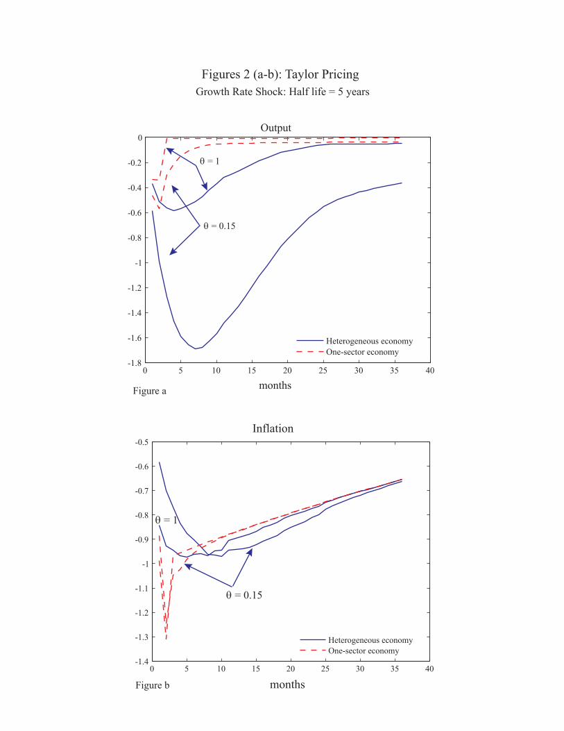
Output

months

θ = 0.15

θ = 1

Inflation

months

θ = 0.15

θ = 1

0 5 10 15 20 25 30 35 40-1.4

-1.3

-1.2

-1.1

-1

-0.9

-0.8

-0.7

-0.6

-0.5

Heterogeneous economyOne-sector economy

0 5 10 15 20 25 30 35 40-1.8

-1.6

-1.4

-1.2

-1

-0.8

-0.6

-0.4

-0.2

0


Figures 2 (a-b): Taylor PricingGrowth Rate Shock: Half life = 5 years

Figure a

Figure b

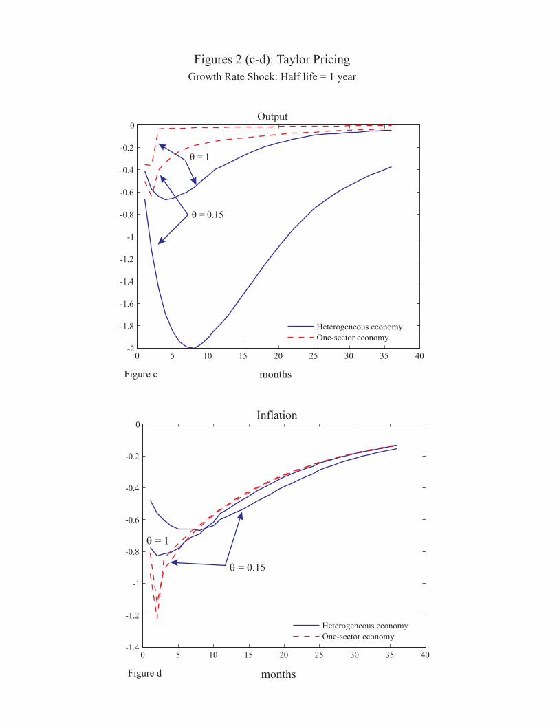
Figures 2 (c-d): Taylor Pricing

Output

months

θ = 0.15

θ = 1

Inflation

months

θ = 0.15

θ = 1

0 5 10 15 20 25 30 35 40-1.4

-1.2

-1

-0.8

-0.6

-0.4

-0.2

0


0 5 10 15 20 25 30 35 40-2

-1.8

-1.6

-1.4

-1.2

-1

-0.8

-0.6

-0.4

-0.2

0


Growth Rate Shock: Half life = 1 year

Figure c

Figure d

heterogeneous price setting behavior and aggregate dynamics: some general...

Documents