heterogeneous peer e ects: a study of education in the
TRANSCRIPT
Heterogeneous Peer Effects: A Study of Education in
the Third World∗
Ashvin Gandhi
Pomona College
Current Version: May 6, 2013
∗I thank Gary Smith, Samuel Antill, and the participants of Gary Smith’s Senior Exercise for their helpfulcomments.
1

Introduction
Many factors contribute to educational outcomes. Undoubtedly, student-specific traits such
as intelligence, socioeconomic status, and parental education play a significant role in student
performance. Additionally, school level resources—textbooks, computers, teachers, etc.—
also affect educational attainment. Student educational outcomes may also be, at least in
part, a function of peer quality. High achieving peers may act as positive role models, while
low achieving ones may act as negative ones.1 A wealth of literature exists that examines
such educational peer effects and their policy implications. Epple et al. (2002), for example,
argues that if high achievers produce positive achievement externalities, then tracking high
achievers with other high achievers stands to harm low achievers in both an absolute and
relative sense: low achievers will perform worse than they would have without tracking, and
the achievement gap between high and low achievers will widen. Peer effects are not strictly
unidirectional, however. Zimmerman (2003), for example, finds that low-achieving college
students may impose a negative externality on their roommates.
Peer effects are not the sole consideration in determining whether to employ tracking.
Duflo et al. (2011) examines a randomized treatment of tracking in Kenyan schools and finds
that in spite of the effects described by Epple et al., tracking benefitted all students because
it allowed teachers to better target their teaching methods to the level of the class. Another
interesting framework through which to examine peer-driven variation is that of competition
with peers. Gneezy et al. (2003), for example, examines how the performance of men and
women differ in competitive environments.
In this paper, I extend previous analyses of peer effects by examining whether these effects
are different for men and women. Strong evidence already exists of positive externalities
from female role models in developing countries. Beaman et al. (2012) found the presence of
female role models in leadership positions in Indian villages substantially shrank the male-
1Additionally, if low achievement imposes a negative externality on other students (e.g. in group projects),there may be a peer-pressure effect as seen in Mas and Morretti (2009).
2

female aspiration gap for both adults and adolescents, erased the educational attainment
gap, and decreased the amount of time that women spent on educational attainment.2 Such
examinations, however, have focused on women in role-model positions rather than in peer
positions. One paper that does examine the role of gender in peer effects is Hoxby (2000),
which examines the role of classroom gender composition in peer effects.
I use two datasets to test the hypothesis that positive educational peer effects are different
for men and women. The first dataset is the Learning and Educational Attainment in Punjab
Schools (LEAPS) dataset, which has been used in a number of educational studies including
Andrabi et al. (2011) and Andrabi et al. (forthcoming). The dataset contains a panel
tracking 34,013 Punjab students’ scores in Urdu, English, and mathematics over a period of
four years. The panel is very unbalanced, however, so I am only able to find a subsample of
5849 students present for testing in the first two years. All of the students examined were in
third grade during the first year of the survey, and almost all of them graduated to fourth
grade in the second year. A small fraction of students—less than 1%—maintained their
status as third graders in the second year but were surveyed because they were still in the
same classroom as their fourth grade peers.3 This is because in some rural Punjab schools,
teachers teach multiple grade levels in the same classroom. I chose to include these students
because their presence in the same classroom may contribute to peer effects, however all of
my results are robust to their exclusion.
The second dataset I use contains student test scores from Western Kenya’s experimental
Extra Teacher Program (ETP).4 Through the ETP, 121 Kenyan primary schools that only
had one first grade teacher were able to hire a second contract teacher for the second term
of the 2005 school year. Of these 121 schools, 60 were asked to assign students into sections
by achievement level while 61 were asked to randomize assignment. Duflo et al. (2011)
2The positive externalizes of higher achieving females do not only affect girls. Andrabi et al. (2012)finds that even minimal maternal education has a substantial positive effect on the educational outcomes forchildren of both genders.
3Both third and fourth grade students took the same test in the second year.4These data can be downloaded from the Jameel Poverty Action Lab (J-PAL) website.
3
compares tracking and non-tracking schools to study the costs and benefits of achievement
tracking. Because I am interested only in peer effects, I restrict my analysis to those 61
schools with random assignment.
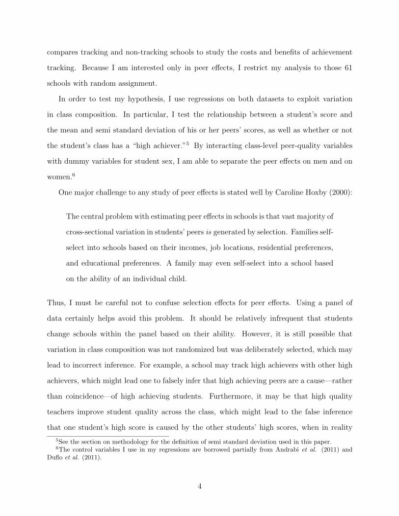
In order to test my hypothesis, I use regressions on both datasets to exploit variation
in class composition. In particular, I test the relationship between a student’s score and
the mean and semi standard deviation of his or her peers’ scores, as well as whether or not
the student’s class has a “high achiever.”5 By interacting class-level peer-quality variables
with dummy variables for student sex, I am able to separate the peer effects on men and on
women.6
One major challenge to any study of peer effects is stated well by Caroline Hoxby (2000):
The central problem with estimating peer effects in schools is that vast majority of
cross-sectional variation in students’ peers is generated by selection. Families self-
select into schools based on their incomes, job locations, residential preferences,
and educational preferences. A family may even self-select into a school based
on the ability of an individual child.
Thus, I must be careful not to confuse selection effects for peer effects. Using a panel of
data certainly helps avoid this problem. It should be relatively infrequent that students
change schools within the panel based on their ability. However, it is still possible that
variation in class composition was not randomized but was deliberately selected, which may
lead to incorrect inference. For example, a school may track high achievers with other high
achievers, which might lead one to falsely infer that high achieving peers are a cause—rather
than coincidence—of high achieving students. Furthermore, it may be that high quality
teachers improve student quality across the class, which might lead to the false inference
that one student’s high score is caused by the other students’ high scores, when in reality
5See the section on methodology for the definition of semi standard deviation used in this paper.6The control variables I use in my regressions are borrowed partially from Andrabi et al. (2011) and
Duflo et al. (2011).
4

the two are caused by the same thing. In order to lessen such problems of endogeneity, I
employ an instrumental variables approach.
Data
In my analysis I use two educational datasets: the first is from the Learning and Educa-
tional Attainment in Punjab Schools (LEAPS) survey, and the second is from Kenya’s Extra
Teacher Program (ETP).
Learning and Educational Attainment in Punjab Schools
The following quotation from the Learning and Educational Attainment in Punjab Schools
(LEAPS) Project website describes the data composition:
The LEAPS Survey consists of data from 823 schools in 112 villages in 3 districts
of Punjab-Attock, Faisalabad and Rahim Yar Khan. These districts represent an
accepted stratification of the province into North (Attock), Central (Faisalabad)
and South (Rahim Yar Khan). The 112 villages in these districts were chosen
randomly from the list of all villages with an existing private school.
These data have been used before to study educational achievement in Pakistan (Andrabi
et al. forthcoming) and teacher value-added metrics (Andrabi et al. 2009).
The LEAPS dataset includes an unbalanced panel of test scores for approximately 34,000
students in rural Punjab schools over four years. Tests were administered near the end of the
school year, allowing sufficient time for students to be affected by their classmates should
peer effects be present.7 Each year, students were given extensive standardized tests in
three key areas: mathematics, English, and Urdu. The questions on these tests were not
7For a smaller sub-sample, highly detailed information on household and demographic information isavailable. I do not make use of this information, however, because it would require me to greatly restrict mysample size.
5

all weighted identically, and the LEAPS Project used a weighting mechanism to develop
test scores in each area that best reflect student performance. I use these test scores in my
analysis and do not modify them in any way, such as by normalizing them.
I restricted the dataset to students who are present in the sample for the first and second
years of the panel, and whose class in the second year had at least fifteen people. I impose the
first restriction because I use statistics from both the first and second years in the regressions.
I impose the second restriction so that the classes are large enough to avoid small-sample
problems with the class-level statistics, especially the class semi standard deviation. After
restricting, there are 5849 students left in the dataset. All of these students were in third
grade in the first year of the panel, and nearly all of these students were in fourth grade
in the second year of the panel. Both third and fourth grade students were given the same
test in the second year. In my exposition, I use the term year to refer to years in the panel
and grade to refer to the child’s school grade. In general, I will refer to the year 1 scores as
baselines cores and the year 2 scores as endline scores.
Table 1 gives student-level summary statistics of test scores, and Table 2 gives other
student-level summary statistics relevant to the analysis. Table 3 gives a summary of
classroom-level statistics. Of particular note is that most students were in either all-male
or all-female classes. Only 1394 of the 5849 students attended coeducational classes. Unfor-
tunately, this prevents me from doing more thorough analyses of co-ed classroom dynamics
using the LEAPS data. For example, it might have been interesting to ask whether girls are
more affected by their female than their male peers.
Extra Teacher Program
With funding from the World Bank, ICS Africa was able to hire an extra first grade teacher
for 140 primary schools in Western Kenya.8 Of these schools, 121 originally only had one
first grade teacher and were able to split that single section into two at the start of the
8ICS stands for Investing in Children and their Societies.
6

second term. Of those 121 schools, 61 were required to randomly assign students into the
two sections. I focus my analysis on these 61 schools, exploiting the randomized variation
in peer-quality caused by the random assignment of students to different teachers.
Before classes were split for the second term, each school assigned its students a first
term score. The material tested in assigning this first term score was not standardized
across schools and are therefore normalized at the school level in the dataset. Still, these
baseline scores provide good proxies for student achievement before the second term and
highly correlate with their performance on standardized tests in mathematics and literature
given at the end of the second term. These second term tests were identical for all schools
participating in the ETP program. In analyzing the ETP dataset, I will usually refer to the
second term standardized test scores as endline scores and the first term scores as baselines
scores. Table 10 gives the summary statistics for student test scores and other variables of
interest.
One key advantage to the ETP dataset over the LEAPS dataset is that the ETP data
come from an experiment and therefore have truly randomized assignment of students to
classes. This controls for a number of factors—such as tracking—that might simultaneously
affect one’s performance and peer quality. Notably, one source of endogeneity that we must
still be careful of is teacher quality.
On the other hand, there a few key disadvantages of the ETP data. First, the ETP data
have been normalized by the Jameel Poverty Action Lab (J-PAL), which hosts the data.
Student test scores were normalized to have a mean of 0 and standard deviation of 1. The
classroom level statistics, however, were normalized using a more complex mechanism that
cannot be reversed and is not entirely transparent in the code from Duflo et al. (2011).
Therefore, one must interpret the results in context of these normalized variables. That the
normalization cannot be reversed prevents determining separate means for men and women
that are consistent with the classroom means present in the J-PAL data. To prevent misuse
of these normalized variables, I closely follow the methodology used by Duflo et al. (2011)
7

in the main analysis of this paper. In Appendix B, however, I analyze within and across
gender peer effects using alternately calculated means.
Methodology
In testing for the effects of high or low achieving students on their peers, I would ideally
like to employ a methodology similar to that in Mas and Moretti (2009). Mas and Moretti
study the effect of high-productivity workers being present on the productivity of generally
low-productivity workers. However, Mas and Moretti have a long panel, while the LEAPS
and ETP panels are very short. The principle, though, remains the same: the regressions
need to control for other factors that may contribute to changes in performance. To do this,
I closely follow the methodology of Duflo et al. (2011) in employing the following regressions
on student endline test scores yij (where i indexes individuals and j indexes class):
yij = α0 + αxij + βbij + λy−ij + εij (1)
yij = α0 + αxij + βbij + λy−ij + λffemaleij × y−ij + εij (2)
yij = α0 + αxij + βbij + λy−ij + γSemiSD(y−ij) + εij (3)
yij = α0 + αxij + βbij + λy−ij + γSemiSD(y−ij) + γffemaleij × SemiSD(y−ij) + εij (4)
yij = α0 + αxij + βbij + λy−ij + ϕHA−ij + εij (5)
8

yij = α0 + αxij + βbij + λy−ij + ϕHA−ij + ϕffemaleij ×HA−ij + εij (6)
In the above equations, x gives a matrix of control variables. In the analysis of the LEAPS
dataset, x includes age, school type (public or private), indicator variables for student and
teacher gender, indicator variables for all-male and all-female classes, and village-level fixed
effects. In the analysis of the ETP dataset, x includes age, an indicator for student gender,
an indicator for whether the teacher was a new ETP hire, and school-level fixed effects. My
choices of controls derive from Andrabi et al. (2009) and Duflo et al. (2011), respectively.
The variable bij gives a student’s baseline test score. In the LEAPS dataset, a student’s
baseline score is taken to be their subject-specific standardized test score in the previous
year. In the ETP dataset, a student’s baseline score is their score from the first term before
the classes were split. It is worth noting that the baseline scores in the ETP dataset are not
standardized across schools, and as such are normalized within each school.
The variables y−ij and SemiSD(y−ij) give the mean and semi standard deviation of
scores received by student i’s classmates. Formally, I define the semi standard deviation as
follows:
SemiSD(yij) =
√√√√ 1
|Classj|∑
ykj>y−ij ,k 6=i
(ykj − y−ij)2.
In other words, I define the semi standard deviation to be the square root of the average
squared distance from the mean for above-average students in student i’s class. This gives a
metric of the dispersion of above average students in student i’s class. A high semi standard
deviation might indicate the presence of outlier students.
Importantly, I exclude student i when calculating statistics with a subscript of −i because
to not do so would bias the coefficients.9 In each of these regressions, I instrument for y−ij
and SemiSD(y−ij) with b−ij and SemiSD(b−ij), respectively, in a two-stage least squares
9For example, if I did not exclude yij from the mean, an increase in yij would actually cause the meanscore to increase. This could lead one to falsely infer that high class means cause high scores when theopposite is true.
9

regression. I employ an instrumental variables approach because y−ij and SemiSD(y−ij) are
likely endogenous, and to simply apply OLS might bias the coefficients and lead to incorrect
inference. For example, good teachers might cause both y−ij and yij to increase. Without
an instrumental variables approach, this would bias the coefficient of y−ij upwards and yield
evidence of peer effects even when none exist.
The variable HA−ij is a dummy variable for at least one of student i’s classmates being
a high achieving student. In the analysis of the LEAPS dataset, I define a high achieving
student to be one whose test score is above the 95th percentile in the sample. Approximately
50% of students in the LEAPS dataset have a high achieving classmate. In the analysis of
the ETP dataset, I define high achievers to be the top performing first grade student at the
school.10 Since each school has two first grade classes that are approximately the same size,
approximately 50% of students in the ETP dataset are in a class with a high achiever. As
with y−ij and SemiSD(y−ij), I instrument for the high achieving variable using a baseline
high achieving variable.
In Equation (1), I test whether peer effects can be detected in correlation achievement
and average peer achievement. This equation is taken directly from Duflo, et al. (2011), who
find evidence of non-gender-specific peer effects in the ETP data. In Equation (2), I try to
differentiate whether average peer score affects males and females differently. In Equation
(3), I allow for the semi standard deviation of peer scores to affect student scores. One
might expect this for a number of reasons. For example, a high semi standard deviation
might indicate the presence of very high performing students, and these strong positive
outliers might be the primary drivers of peer effects. If this is the case, the coefficients in
Equation (3) will have significant implications for how to group students to optimize positive
peer effects. Alternatively, it may be that teacher efficacy is a function of the variance of
student achievement—e.g. Duflo et al. (2011) suggests that teachers are more effective at
teaching classes with a lower variance of achievement. Equation (4) tests whether the semi
10High achievers cannot be defined using percentiles in the ETP dataset because the baseline scores arenot standardized across schools.
10

standard deviation of classmate scores affects males and females differently. Equation (5)
tests whether high achievers drive peer effects, and Equation (6) tests whether high achiever
effects are different for men and women.
I run each of these regressions three times for each dataset—once for each dependent
variable of interest. In the LEAPS analysis, the dependent variables are math score, English
score, and Urdu score. In the ETP analysis, the dependent variables are math score, liter-
ature score, and total score. In all regressions using the LEAPS data, standard errors are
clustered at the village level, and in all regressions using the ETP data, standard errors are
clustered at the school level.
Results
Learning and Educational Attainment in Punjab Schools
Tables 4, 5, and 6 give the results of the LEAPS regressions without using instrumental
variables. These regressions consistently show large statistically significant coefficients for
the class mean variable but not for the same variable interacted with the female dummy
variable. Notably these coefficients are largest for math, second largest for English, and
smallest for Urdu. Still, even the smallest coefficients are quite large. In general these
results indicate that a 1 point increase in the average peer score correlates with a .4 to .7
point increase in a student’s scores. It is likely that these very high coefficients are the result
of achievement tracking, self-selection, and other sources of endogeneity. Interestingly, the
coefficient on the female interacted class mean variable is not statistically significant in any
of the regressions.
The coefficients of the semi standard deviation variables are consistently negative with
very large coefficients. As with the coefficients on the class mean variable, this result should
be interpreted cautiously. The coefficient on the semi standard deviation variable may be
significant because having a greater spread of above average students reduces peer effects,
11

but it may simply be evidence of other patterns—e.g. that students of better teachers have
lower variance outcomes. Notably, the negative relationship between test scores and the peer
semi standard deviation appears much stronger for men than for women.
The coefficients of the dummy for having a high achiever in the classroom is always
negative with large magnitudes and statistical significance. This might indicate that high
achievers do not produce positive peer effects in proportion to how much they increase
the class mean—i.e., fixing mean classmate score, high achievers have a negative effect on
their peers. As with the mean and semi standard deviation, the coefficient may be driven
by endogenous factors. For example, good teachers might produce high achievers while
simultaneously improving the scores of all students. The female-interacted high achievement
variable is only statistically significant in the case of math scores, in which case it is large
and positive.
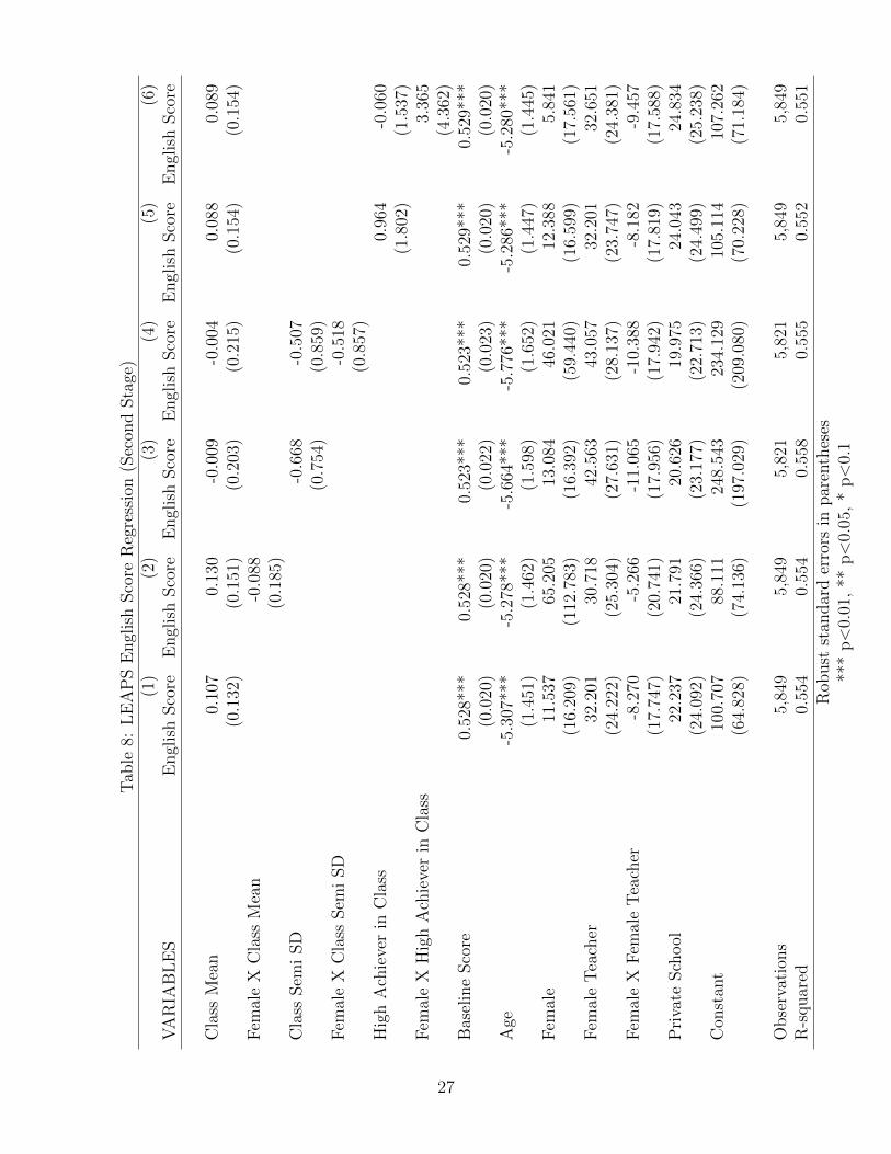
Tables 7, 8, and 9 give the results of the LEAPS regressions when a two-stage least
squares, instrumental variables approach is applied.11 While the application of instrumental
variables should mitigate many sources of endogeneity in our variables of interest, the large
standard errors in these regressions prevent inference about peer effects. All of the coefficients
regarding peer effects become statistically insignificant in these regressions, and the signs of
the coefficient are not always consistent with the regressions without instruments—e.g. the
coefficients for the class mean are generally negative in the two stage least squares regression,
while they were consistently positive when no instruments were used.
These results shed doubts on the reliability of the coefficients seen in the analysis without
instruments. They should not be taken as positive evidence that peer effects do not exist.
The standard errors of the coefficients in the two stage least squares regressions are very
large, and therefore, it may be that peer effects exist, but the standard errors are simply too
large to detect these effects. Little can be done to correct this here, and I hope to perform
11I do not include the first stages, however, I did a joint-significance test on the instruments in eachfirst-stage regression and found that the instruments were quite strong (the p-value associated with theF-statistics were all less than .0001).
12

similar analyses with larger datasets in the future. We can say with confidence, however,
that peer effects in these data are not strong enough to be discernable when applying an
instrumental variables approach.
While these regressions do not provide any conclusive evidence of peer effects—let alone
heterogeneity in peer effects—I do find that some of the control variables are consistently
significant in the regressions. Most notably, baseline scores consistently have a strong and
statistically significant positive relationship with endline scores. Since the baseline scores
were previous year scores, this likely reflects that prior ability strongly correlates with current
ability. That the coefficient of one’s baseline score is less than 1 indicates a regression to the
mean of student test scores. This phenomenon is commonly known—see for example Mee
and Chua (1991)—and does not cause any further problems for inference. Additionally, I
find age to consistently have a negative relationship with test scores. This may be because
students who are young for their grade and skipped a grade are likely high-ability, high
achieving students, while those who are old for their grade are likely low-ability, low achieving
students.
Extra Teacher Program
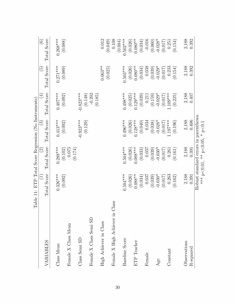
Tables 11, 12, and 13 give the results of the ETP regressions without using instrumental
variables. The results in these regressions can be interpreted less cautiously than those in
the LEAPS regressions without instruments because the ETP enforced random assignment
of students to teachers. Therefore, self-selection cannot bias the coefficients. Still, there is
some cause for concern because the effects of teacher quality might still yield problems of
endogeneity in the model.
In these regressions, I find large, statistically significant positive coefficients for the class
mean variable. Because the class mean variable has been normalized in a complex manner,
it is important to interpret its regression coefficient in context of the variable mean and stan-
dard deviation: .00009 and .1056, respectively. Therefore, for example, we should interpret
13

a regression coefficient of .5 as meaning that a one standard deviation increase in average
classmate quality leads to a .05 standard deviation increase in a student’s achievement.
Therefore, while the coefficients are very large, the peer effects they describe are actually
much smaller: the coefficients generally indicate that a one standard deviation increase in
the average peer score yields a .02 to .04 standard deviation increase in a student’s score.
These weak peer effects generally appear stronger for math scores than for literature scores.
There is little evidence from these regressions that these small peer effects differ between
women and men.
I find the class semi standard deviation variable to be consistently negative and statis-
tically significant.12 As before, while this may suggest that greater spread of above average
students reduces peer effects, it may also be the result of students of better teachers having
lower variance outcomes. In the case of math scores, there is some evidence that the negative
effect of the semi standard deviation of classmates is larger for women.
Regression (5) in both the math and total score regressions indicates that a high achieving
student may have positive peer effects more than in proportion to how much they increase
the class mean—i.e. fixing mean classmate score, high achievers improve their peers’ perfor-
mances by about .05 standard deviations. If these effects are believed, then the peer effects
of a high achiever on his peers’ math scores is greater than the peer effects produced by
a one standard deviation increase in the average peer math score. These effects, however,
are not statistically significant in regression (6), when a gender-interacted high achievement
variable is included.
Tables 14, 15, and 16 give the results of the LEAPS regressions when a two-stage least
squares, instrumental variables approach is applied.13 While the application of instrumental
variables mitigates problems of endogeneity, it does also reduce the efficiency of the coefficient
estimators, increasing the standard errors. Noticeably, many of the coefficients regarding peer
12While the coefficient of this variable are large, the effects they imply are much more reasonable in contextof the means and standard deviations of the semi standard deviation.
13I do not include the first stages, however they all show that the instruments are very strong (p valuesless than .0001).
14

effects become statistically insignificant in these regressions. The sole exception is that the
class mean variable consistently shows coefficients that are consistently positive and generally
statistically significant. As before, while these coefficients are large, they generally imply
relatively small peer effects: a one standard deviation increase in the average peer score
generally yields a .04 to .06 standard deviation increase in a student’s score. The result is
most robust in math scores, where it is at least statistically significant at the 10 percent level
in all of the regressions. Where the class mean is found insignificant, it is usually due to very
large standard errors. Notably, the regressions do not discern any statistically significant
difference in how average peer achievement affects males and females. However, this may
be driven by the fact that the standard errors are large while the peer effects in general are
very small, making it difficult to discern a difference should one exist.
The class semi standard deviation variable, though generally insignificant, is consistently
positive and even statistically significant at the 10 percent level in regression (3) of Table 15.
Its coefficient of nearly .6 is seemingly large, but taken in context of the standard deviation
of the class semi standard deviation, which is .19, the coefficient actually describes quite a
small effect. These results cast doubt on the large negative coefficients seen in Tables 11, 12,
and 13. The regressions do not discern any statistically significant difference in the way that
males and females are affected by the semi standard deviation of their classmates, but this
may be the result of large standard errors. None of the regressions find statistically significant
evidence that high achievers drive peer effects. This also, may be driven by relatively small
effects and large standard errors.
As in the LEAPS regression we find that some control variables are consistently signif-
icant. Most notably, baseline score consistently has a strong and statistically significant
positive relationship with student scores. This again likely reflects the persistence of innate
abilities from the baseline period into the testing period. Notably, the baseline score co-
efficients tend to be lower in the ETP regressions than in the LEAPS regressions. This is
likely because LEAPS baseline tests were standardized, subject-specific, and highly similar
15

to the endline tests, while the ETP tests were not. Therefore, the LEAPS baseline test
scores likely better correlate with aptitude for the endline tests than do the ETP baseline
scores. We also once again find age to consistently have a negative relationship with test
scores. This likely holds for the same reason in the ETP data as it did in the LEAPS data.
We also find evidence that the new ETP hires tend to improve student performance. This
is consistent with the findings of Duflo et al., who argue that the finding evidences poor
incentive structures for Kenyan teachers who are not new hires.
Conclusion
My results from analyzing the LEAPS data are generally inconclusive: I do not find any
evidence of peer effects that are robust to the use of an instrumental variables approach, but
this may simply be the result of large standard errors. The results from analyzing the ETP
data are more promising: I find some robust evidence of weak peer effects that positively
correlate with mean peer achievement. Namely, a 1 standard deviation increase in mean
peer quality yields approximately a .04 to .06 increase in student achievement through peer
effects. In my instrumental variable analysis, I do not find any evidence of robust differences
in how peer quality affects men and women. If gender heterogeneity in peer effects exist,
they are not large enough to be discernable from the ETP dataset. Even when instrumental
variables are not used, there is little to no evidence of different effects for men and women.
While this indicates that such heterogeneity likely does not exist or is too small to detect,
further analysis using larger datasets and yielding smaller standard errors would help to
determine this more conclusively. If my results are to be believed, then peer effects are likely
too small to be a major factor in education policy, and the differences between peer effects
for men and women certainly are.
While my analysis does not conclusively answer the questions about heterogeneity in
peer effects, it does provide testament to three important things. The first is the importance
16

of instrumental variables where endogeneity is suspected, for many of my results were not
robust to the use of instruments. The second is the importance of very large datasets when
analyzing such questions, for frequently my inference was hindered by large standard errors.
The third is the value of experiments in isolating desired variation. I am better able to detect
peer effects in the ETP dataset, even though it was smaller than the LEAPS dataset, likely
because the ETP data derived from a randomized experiment while the LEAPS data did
not.
References
Andrabi, Tahir, Jishnu Das, Asim Ijaz Khwaja, and Tristan Zajonc. 2011. “Do Value-Added
Estimates Add Value? Accounting for Learning Dynamics.” American Economic Journal:
Applied Economics, 3(3): 29-54.
Andrabi, Tahir, Jishnu Das, and Asim Ijaz Khwaja. 2012. “What Did You Do All Day?:
Maternal Education and Child Outcomes.” Journal of Human Resources 47(4): 873-912.
Beaman, L., Duflo, E., Pande, R., and Topalova, P. (2012). “Female leadership raises aspi-
rations and educational attainment for girls: A policy experiment in India.” Science, 335,
582586.
Duflo, Esther, Pascaline Dupas, and Michael Kremer. 2011. “Peer Effects, Teacher Incen-
tives, and the Impact of Tracking: Evidence from a Randomized Evaluation in Kenya,”
American Economic Review, 101(5): 1739-74.
Epple, Dennis, Elizabeth Newlon, and Richard Romano. 2002. “Ability Tracking, School
Competition, and the Distribution of Educational Benefits.” Journal of Public Economics,
17
83(1): 148.
Gneezy, Uri, Muriel Niederle, and Aldo Rustichini. 2003. “Performance in Competitive
Environments: Gender Differences.” Quarterly Journal of Economics, 118(3): 1049-1074.
Hoxby, Caroline. 2000. “Peer Effects in the Classroom: Learning from Gender and Race
Variation.” National Bureau of Economic Research Working Paper 7867.
Learning and Educational Achievement in Punjab Schools (LEAPS):Insights to Inform the
Policy Debate. Forthcoming, Oxford University Press: (Joint with Jishnu Das, Asim Ijaz
Khwaja, Tara Vishwanath and Tristan Zajonc.)
Mas, Alexander and Enrico Moretti. 2009. “Peers at Work.” American Economic Review,
99(1): 112-145.
Mee, Robert W. and Tin Chiu Chua. 1991. ”Regression toward the mean and the paired
sample t test.” The American Statistician 45(1): 39-42.
Zimmerman, David. 2003. “Peer Effects in Academic Outcomes: Evidence form a Natural
Experiment.” Review of Economics and Statistics, 85(1), 9-23.
18

Appendix A
Table 1: Student-level Score Summary Statistics
All Students, N=5849Variable Mean Std. Dev. Min MaxMath Score (Year 2) 541.52 144.58 24.47 941.99Math Score (Year 1) 519.74 128.45 6.16 903.70English Score (Year 2) 535.89 136.49 38.53 962.86English Score (Year 1) 505.59 135.70 0.49 905.08Urdu Score (Year 2) 549.90 142.79 22.26 1000.00Urdu Score (Year 1) 513.80 134.40 20.41 922.97
At Boys’ Schools, N=2501Variable Mean Std. Dev. Min MaxMath Score (Year 2) 538.74 150.15 24.47 867.65Math Score (Year 1) 516.28 128.12 6.16 854.12English Score (Year 2) 484.43 146.20 38.53 877.10English Score (Year 1) 460.44 138.17 0.49 815.93Urdu Score (Year 2) 514.46 154.29 22.26 896.38Urdu Score (Year 1) 482.75 141.65 20.41 922.97
At Girls’ Schools, N = 1954Variable Mean Std. Dev. Min MaxMath Score (Year 2) 498.71 142.17 24.47 852.81Math Score (Year 1) 494.11 137.48 6.16 903.70English Score (Year 2) 530.74 105.79 38.53 839.98English Score (Year 1) 492.42 115.62 54.88 870.61Urdu Score (Year 2) 543.46 130.23 22.26 975.40Urdu Score (Year 1) 511.80 130.82 20.41 888.32
At Coed Schools, N = 1394Variable Mean Std. Dev. Min MaxMath Score (Year 2) 606.51 110.21 62.69 941.99Math Score (Year 1) 561.90 102.90 58.10 792.30English Score (Year 2) 635.44 97.24 38.53 962.86English Score (Year 1) 605.06 102.44 76.51 905.08Urdu Score (Year 2) 622.52 107.22 22.26 1000.00Urdu Score (Year 1) 572.30 103.30 35.47 865.12
19

Table 2: Other Student-level Summary Statistics, N = 5849
Variable Mean Std. Dev. Min MaxFemale 0.44 0.50 0 1Female Teacher 0.51 0.50 0 1Private School 0.19 0.39 0 1Age (Year 2) 10.44 1.40 7 17.83Grade (Year 2) 3.99 0.07 3 4Class Size 27.68 13.05 15 92Girls’ School 0.33 0.47 0 1Boys’ School 0.43 0.49 0 1
20

Table 3: Classroom Summary Statistics
All Schools, N = 243Variable Mean Std. Dev. Min MaxMean Math (Year 2) 542.96 88.06 324.28 806.32Mean Math (Year 1) 520.31 83.00 278.59 735.66Mean English (Year 2) 537.21 98.85 195.17 776.99Mean English (Year 1) 505.61 106.25 89.15 732.37Mean Urdu (Year 2) 550.17 84.69 233.33 832.48Mean Urdu (Year 1) 512.90 86.25 90.54 693.02SD Math (Year 2) 542.96 88.06 324.28 806.32SD Math (Year 1) 95.57 28.90 30.91 188.19SD English (Year 2) 92.39 32.79 41.43 200.84SD English (Year 1) 88.35 26.91 37.37 163.36SD Urdu (Year 2) 111.85 35.71 35.11 221.96SD Urdu (Year 1) 101.80 34.83 46.10 216.92Semi SD Math (Year 2) 101.95 31.25 38.33 185.90Semi SD Math (Year 1) 87.17 27.08 23.88 170.47Semi SD English (Year 2) 82.95 29.99 33.45 227.21Semi SD English (Year 1) 81.25 26.33 35.44 194.48Semi SD Urdu (Year 2) 101.17 30.27 35.52 190.34Semi SD Urdu (Year 1) 92.38 33.61 36.24 284.24
Boys’ Schools, N = 103Variable Mean Std. Dev. Min MaxMean Math (Year 2) 538.87 89.72 324.28 716.05Mean Math (Year 1) 514.70 78.23 309.74 735.66Mean English (Year 2) 483.95 98.35 195.17 705.91Mean English (Year 1) 455.19 104.15 89.15 715.91Mean Urdu (Year 2) 513.98 85.77 233.33 729.27Mean Urdu (Year 1) 479.59 87.87 90.54 693.02SD Math (Year 2) 538.87 89.72 324.28 716.05SD Math (Year 1) 100.28 27.37 43.44 188.19SD English (Year 2) 108.56 36.05 41.43 200.84SD English (Year 1) 95.59 28.69 43.51 163.36SD Urdu (Year 2) 127.68 36.85 65.38 221.96SD Urdu (Year 1) 112.31 32.55 57.25 196.34Semi SD Math (Year 2) 111.77 31.49 57.79 185.90Semi SD Math (Year 1) 88.80 25.56 35.86 170.47Semi SD English (Year 2) 96.59 35.88 44.88 227.21Semi SD English (Year 1) 88.08 29.41 39.28 194.48Semi SD Urdu (Year 2) 111.87 30.63 51.62 190.34Semi SD Urdu (Year 1) 101.88 37.62 48.77 284.24
21

Table 3 ContinuedGirls’ Schools, N = 77
Variable Mean Std. Dev. Min MaxMean Math (Year 2) 499.47 76.81 334.18 676.17Mean Math (Year 1) 493.13 90.88 278.59 709.38Mean English (Year 2) 530.81 55.78 427.98 653.04Mean English (Year 1) 492.49 75.39 334.82 695.55Mean Urdu (Year 2) 541.98 64.84 379.39 675.37Mean Urdu (Year 1) 509.89 79.44 325.59 666.28SD Math (Year 2) 499.47 76.81 334.18 676.17SD Math (Year 1) 102.81 31.22 30.91 178.19SD English (Year 2) 88.28 25.05 48.61 145.18SD English (Year 1) 90.23 23.76 38.42 157.19SD Urdu (Year 2) 110.02 32.17 40.18 192.67SD Urdu (Year 1) 102.34 38.80 47.22 216.92Semi SD Math (Year 2) 105.29 28.60 45.48 180.09Semi SD Math (Year 1) 94.70 30.04 23.88 159.62Semi SD English (Year 2) 78.93 19.31 44.89 123.37Semi SD English (Year 1) 82.40 23.23 38.78 148.46Semi SD Urdu (Year 2) 100.84 29.58 43.57 186.25Semi SD Urdu (Year 1) 92.18 32.18 36.24 182.38
Coed Schools, N = 63Variable Mean Std. Dev. Min MaxMean Math (Year 2) 602.79 61.48 480.98 806.32Mean Math (Year 1) 562.69 62.49 403.09 691.25Mean English (Year 2) 632.10 67.08 379.99 776.99Mean English (Year 1) 604.07 70.46 388.88 732.37Mean Urdu (Year 2) 619.33 60.18 485.37 832.48Mean Urdu (Year 1) 571.02 57.54 451.03 668.25SD Math (Year 2) 602.79 61.48 480.98 806.32SD Math (Year 1) 79.00 21.25 41.14 138.17SD English (Year 2) 70.95 19.19 44.50 127.34SD English (Year 1) 74.22 22.06 37.37 128.87SD Urdu (Year 2) 88.18 22.03 35.11 155.00SD Urdu (Year 1) 83.97 25.32 46.10 162.07Semi SD Math (Year 2) 81.81 24.33 38.33 157.76Semi SD Math (Year 1) 75.30 21.54 37.08 135.72Semi SD English (Year 2) 65.54 17.32 33.45 129.66Semi SD English (Year 1) 68.87 19.87 35.44 119.14Semi SD Urdu (Year 2) 84.08 21.74 35.52 149.16Semi SD Urdu (Year 1) 77.11 20.63 38.92 134.95
22

Tab
le4:
LE
AP
SM
ath
Sco
reR
egre
ssio
n(N
oIn
stru
men
ts)
(1)
(2)
(3)
(4)
(5)
(6)
VA
RIA
BL
ES
Mat
hSco
reM
ath
Sco
reM
ath
Sco
reM
ath
Sco
reM
ath
Sco
reM
ath
Sco
re
Cla
ssM
ean
0.58
4***
0.59
9***
0.47
7***
0.49
6***
0.68
3***
0.67
9***
(0.0
59)
(0.0
67)
(0.0
80)
(0.0
82)
(0.0
63)
(0.0
64)
Fem
ale
XC
lass
Mea
n-0
.035
(0.0
80)
Cla
ssSem
iSD
-0.5
25**
*-0
.683
***
(0.1
44)
(0.1
52)
Fem
ale
XC
lass
Sem
iSD
0.52
2***
(0.1
91)
Hig
hA
chie
ver
inC
lass
-7.5
31**
*-9
.108
***
(1.1
66)
(1.2
11)
Fem
ale
XH
igh
Ach
ieve
rin
Cla
ss4.
779*
**(1
.626
)B
asel
ine
Sco
re0.
532*
**0.
533*
**0.
526*
**0.
525*
**0.
531*
**0.
532*
**(0
.031
)(0
.031
)(0
.031
)(0
.030
)(0
.030
)(0
.030
)A
ge-6
.293
***
-6.2
83**
*-6
.200
***
-6.0
84**
*-6
.286
***
-6.2
72**
*(1
.399
)(1
.398
)(1
.422
)(1
.396
)(1
.385
)(1
.380
)F
emal
e-3
1.96
9*-1
0.49
2-3
1.02
8*-7
6.85
8***
-29.
364
-38.
064*
*(1
7.77
6)(5
4.60
2)(1
7.67
5)(2
6.03
7)(1
8.97
3)(1
9.04
3)F
emal
eT
each
er-2
4.92
5-2
4.98
9-2
4.16
4-2
3.52
0-2
2.22
3-2
0.89
1(1
5.33
7)(1
5.30
7)(1
7.01
2)(1
6.17
6)(1
6.55
5)(1
7.01
0)F
emal
eX
Fem
ale
Tea
cher
33.7
1033
.540
33.0
3832
.995
29.0
2831
.105
(20.
600)
(20.
777)
(20.
483)
(21.
060)
(21.
568)
(20.
792)
Pri
vate
Sch
ool
12.8
5212
.315
4.67
92.
764
6.66
58.
690
(9.1
97)
(9.1
81)
(10.
931)
(10.
712)
(10.
818)
(10.
905)
Con
stan
t-2
9.22
1-3
6.98
588
.033
*85
.547
*-7
2.91
8**
-71.
653*
*(2
8.86
0)(3
1.32
9)(4
5.94
2)(4
7.65
1)(3
0.85
8)(3
0.65
0)
Obse
rvat
ions
5,84
95,
849
5,84
95,
849
5,84
95,
849
R-s
quar
ed0.
483
0.48
40.
488
0.49
00.
488
0.48
9R
obust
stan
dar
der
rors
inpar
enth
eses
***
p<
0.01
,**
p<
0.05
,*
p<
0.1
23

Tab
le5:
LE
AP
SE
ngl
ish
Sco
reR
egre
ssio
n(N
oIn
stru
men
ts)
(1)
(2)
(3)
(4)
(5)
(6)
VA
RIA
BL
ES
Engl
ish
Sco
reE
ngl
ish
Sco
reE
ngl
ish
Sco
reE
ngl
ish
Sco
reE
ngl
ish
Sco
reE
ngl
ish
Sco
re
Cla
ssM
ean
0.54
6***
0.54
3***
0.42
6***
0.43
4***
0.60
8***
0.60
8***
(0.0
70)
(0.0
86)
(0.0
59)
(0.0
58)
(0.0
75)
(0.0
75)
Fem
ale
XC
lass
Mea
n0.
013
(0.0
93)
Cla
ssSem
iSD
-0.6
01**
*-0
.715
***
(0.1
67)
(0.1
83)
Fem
ale
XC
lass
Sem
iSD
0.63
2**
(0.2
91)
Hig
hA
chie
ver
inC
lass
-4.2
90**
*-4
.343
***
(0.8
44)
(0.9
07)
Fem
ale
XH
igh
Ach
ieve
rin
Cla
ss0.
171
(0.8
32)
Bas
elin
eSco
re0.
459*
**0.
459*
**0.
456*
**0.
457*
**0.
458*
**0.
458*
**(0
.032
)(0
.032
)(0
.030
)(0
.027
)(0
.031
)(0
.031
)A
ge-4
.839
***
-4.8
43**
*-5
.124
***
-5.0
61**
*-4
.952
***
-4.9
51**
*(1
.080
)(1
.069
)(1
.128
)(1
.092
)(1
.072
)(1
.072
)F
emal
e0.
093
-7.8
631.
964
-42.
855
-3.1
57-3
.491
(15.
337)
(59.
333)
(15.
370)
(25.
844)
(14.
936)
(15.
536)
Fem
ale
Tea
cher
0.64
70.
835
11.2
2113
.293
2.13
32.
157
(10.
402)
(10.
953)
(11.
512)
(11.
318)
(11.
653)
(11.
686)
Fem
ale
XF
emal
eT
each
er9.
425
8.99
86.
208
7.27
78.
197
8.13
2(1
7.01
1)(1
7.18
1)(1
6.96
0)(1
9.20
5)(1
6.44
1)(1
6.33
3)P
riva
teSch
ool
-5.6
34-5
.595
-5.9
09-6
.269
-12.
358
-12.
320
(6.9
98)
(7.0
81)
(8.4
18)
(8.3
97)
(7.6
03)
(7.6
40)
Con
stan
t-3
2.80
1*-3
1.06
810
5.39
4**
96.2
07**
-46.
129*
*-4
6.02
6**
(18.
894)
(22.
880)
(43.
717)
(40.
507)
(18.
584)
(18.
648)
Obse
rvat
ions
5,84
95,
849
5,84
95,
849
5,84
95,
849
R-s
quar
ed0.
580
0.58
00.
585
0.58
70.
583
0.58
3R
obust
stan
dar
der
rors
inpar
enth
eses
***
p<
0.01
,**
p<
0.05
,*
p<
0.1
24

Tab
le6:
LE
AP
SU
rdu
Sco
reR
egre
ssio
n(N
oIn
stru
men
ts)
(1)
(2)
(3)
(4)
(5)
(6)
VA
RIA
BL
ES
Urd
uSco
reU
rdu
Sco
reU
rdu
Sco
reU
rdu
Sco
reU
rdu
Sco
reU
rdu
Sco
re
Cla
ssM
ean
0.49
4***
0.49
2***
0.42
4***
0.44
1***
0.60
0***
0.59
9***
(0.0
80)
(0.1
03)
(0.0
88)
(0.0
87)
(0.0
88)
(0.0
88)
Fem
ale
XC
lass
Mea
n0.
004
(0.0
98)
Cla
ssSem
iSD
-0.4
35**
*-0
.578
***
(0.1
51)
(0.1
88)
Fem
ale
XC
lass
Sem
iSD
0.46
6**
(0.2
21)
Hig
hA
chie
ver
inC
lass
-8.2
40**
*-7
.821
***
(1.4
63)
(1.4
88)
Fem
ale
XH
igh
Ach
ieve
rin
Cla
ss-0
.862
(1.6
37)
Bas
elin
eSco
re0.
544*
**0.
544*
**0.
538*
**0.
538*
**0.
544*
**0.
544*
**(0
.032
)(0
.032
)(0
.032
)(0
.031
)(0
.031
)(0
.031
)A
ge-6
.612
***
-6.6
13**
*-6
.404
***
-6.2
80**
*-6
.634
***
-6.6
17**
*(1
.260
)(1
.247
)(1
.292
)(1
.271
)(1
.212
)(1
.213
)F
emal
e14
.918
12.5
4515
.495
-25.
150
15.8
3317
.452
(12.
441)
(60.
122)
(12.
441)
(24.
805)
(12.
485)
(12.
542)
Fem
ale
Tea
cher
8.62
78.
661
14.2
9216
.056
11.1
0510
.871
(13.
862)
(14.
245)
(13.
301)
(12.
906)
(13.
746)
(13.
879)
Fem
ale
XF
emal
eT
each
er-2
.524
-2.5
86-2
.829
-2.6
82-4
.086
-4.1
53(1
4.33
8)(1
4.56
5)(1
4.48
1)(1
5.40
2)(1
4.31
9)(1
4.46
2)P
riva
teSch
ool
1.24
31.
301
0.13
9-1
.844
-6.1
94-6
.357
(9.8
05)
(10.
173)
(10.
614)
(10.
428)
(12.
637)
(12.
609)
Con
stan
t-3
5.10
6-3
4.46
550
.544
50.6
32-7
9.09
6**
-79.
649*
*(3
1.96
2)(3
8.78
3)(4
6.43
6)(4
6.46
8)(3
5.22
3)(3
5.54
3)
Obse
rvat
ions
5,84
95,
849
5,84
95,
849
5,84
95,
849
R-s
quar
ed0.
495
0.49
50.
498
0.50
00.
501
0.50
1R
obust
stan
dar
der
rors
inpar
enth
eses
***
p<
0.01
,**
p<
0.05
,*
p<
0.1
25

Tab
le7:
LE
AP
SM
ath
Sco
reR
egre
ssio
n(S
econ
dSta
ge)
(1)
(2)
(3)
(4)
(5)
(6)
VA
RIA
BL
ES
Mat
hSco
reM
ath
Sco
reM
ath
Sco
reM
ath
Sco
reM
ath
Sco
reM
ath
Sco
re
Cla
ssM
ean
-0.3
93-0
.248
-0.2
15-0
.198
-0.6
13-0
.658
(0.3
18)
(0.3
02)
(0.3
21)
(0.3
18)
(0.5
86)
(0.6
11)
Fem
ale
XC
lass
Mea
n-0
.309
(0.4
08)
Cla
ssSem
iSD
0.90
50.
762
(1.1
65)
(1.0
61)
Fem
ale
XC
lass
Sem
iSD
0.63
7(1
.694
)H
igh
Ach
ieve
rin
Cla
ss13
.008
27.0
97(2
1.16
0)(2
5.22
3)F
emal
eX
Hig
hA
chie
ver
inC
lass
-34.
696
(34.
661)
Bas
elin
eSco
re0.
611*
**0.
610*
**0.
622*
**0.
624*
**0.
616*
**0.
619*
**(0
.025
)(0
.025
)(0
.026
)(0
.027
)(0
.025
)(0
.026
)A
ge-7
.883
***
-7.7
63**
*-8
.055
***
-8.0
44**
*-7
.977
***
-8.1
47**
*(2
.181
)(2
.130
)(2
.241
)(2
.246
)(2
.387
)(2
.539
)F
emal
e-1
.403
188.
263
-2.8
14-5
4.84
5-4
.338
59.1
65(2
5.15
4)(2
52.7
19)
(24.
486)
(140
.854
)(2
1.37
1)(7
6.41
7)F
emal
eT
each
er19
.363
17.9
3918
.358
17.7
9916
.964
8.15
8(4
1.87
6)(4
0.52
1)(4
0.81
0)(3
9.99
7)(3
8.95
6)(3
5.87
3)F
emal
eX
Fem
ale
Tea
cher
-2.0
90-2
.898
-1.1
80-0
.020
4.16
3-1
0.74
1(2
7.80
0)(2
8.50
6)(2
7.63
1)(2
8.58
2)(2
4.71
7)(4
2.35
3)P
riva
teSch
ool
57.4
6051
.838
71.8
6071
.636
70.4
3059
.716
(40.
684)
(37.
431)
(54.
039)
(55.
236)
(44.
854)
(43.
050)
Con
stan
t37
2.69
5**
296.
138*
173.
355
168.
656
468.
740*
491.
313*
(159
.699
)(1
55.4
53)
(248
.882
)(2
48.7
52)
(276
.963
)(2
89.8
87)
Obse
rvat
ions
5,84
95,
849
5,84
95,
849
5,84
95,
849
R-s
quar
ed0.
364
0.36
50.
335
0.32
50.
321
0.26
2R
obust
stan
dar
der
rors
inpar
enth
eses
***
p<
0.01
,**
p<
0.05
,*
p<
0.1
26
Tab
le8:
LE
AP
SE
ngl
ish
Sco
reR
egre
ssio
n(S
econ
dSta
ge)
(1)
(2)
(3)
(4)
(5)
(6)
VA
RIA
BL
ES
Engl
ish
Sco
reE
ngl
ish
Sco
reE
ngl
ish
Sco
reE
ngl
ish
Sco
reE
ngl
ish
Sco
reE
ngl
ish
Sco
re
Cla
ssM
ean
0.10
70.
130
-0.0
09-0
.004
0.08
80.
089
(0.1
32)
(0.1
51)
(0.2
03)
(0.2
15)
(0.1
54)
(0.1
54)
Fem
ale
XC
lass
Mea
n-0
.088
(0.1
85)
Cla
ssSem
iSD
-0.6
68-0
.507
(0.7
54)
(0.8
59)
Fem
ale
XC
lass
Sem
iSD
-0.5
18(0
.857
)H
igh
Ach
ieve
rin
Cla
ss0.
964
-0.0
60(1
.802
)(1
.537
)F
emal
eX
Hig
hA
chie
ver
inC
lass
3.36
5(4
.362
)B
asel
ine
Sco
re0.
528*
**0.
528*
**0.
523*
**0.
523*
**0.
529*
**0.
529*
**(0
.020
)(0
.020
)(0
.022
)(0
.023
)(0
.020
)(0
.020
)A
ge-5
.307
***
-5.2
78**
*-5
.664
***
-5.7
76**
*-5
.286
***
-5.2
80**
*(1
.451
)(1
.462
)(1
.598
)(1
.652
)(1
.447
)(1
.445
)F
emal
e11
.537
65.2
0513
.084
46.0
2112
.388
5.84
1(1
6.20
9)(1
12.7
83)
(16.
392)
(59.
440)
(16.
599)
(17.
561)
Fem
ale
Tea
cher
32.2
0130
.718
42.5
6343
.057
32.2
0132
.651
(24.
222)
(25.
304)
(27.
631)
(28.
137)
(23.
747)
(24.
381)
Fem
ale
XF
emal
eT
each
er-8
.270
-5.2
66-1
1.06
5-1
0.38
8-8
.182
-9.4
57(1
7.74
7)(2
0.74
1)(1
7.95
6)(1
7.94
2)(1
7.81
9)(1
7.58
8)P
riva
teSch
ool
22.2
3721
.791
20.6
2619
.975
24.0
4324
.834
(24.
092)
(24.
366)
(23.
177)
(22.
713)
(24.
499)
(25.
238)
Con
stan
t10
0.70
788
.111
248.
543
234.
129
105.
114
107.
262
(64.
828)
(74.
136)
(197
.029
)(2
09.0
80)
(70.
228)
(71.
184)
Obse
rvat
ions
5,84
95,
849
5,82
15,
821
5,84
95,
849
R-s
quar
ed0.
554
0.55
40.
558
0.55
50.
552
0.55
1R
obust
stan
dar
der
rors
inpar
enth
eses
***
p<
0.01
,**
p<
0.05
,*
p<
0.1
27

Tab
le9:
LE
AP
SU
rdu
Sco
reR
egre
ssio
n(S
econ
dSta
ge)
(1)
(2)
(3)
(4)
(5)
(6)
VA
RIA
BL
ES
Urd
uSco
reU
rdu
Sco
reU
rdu
Sco
reU
rdu
Sco
reU
rdu
Sco
reU
rdu
Sco
re
Cla
ssM
ean
-0.2
36-0
.208
-0.3
38-0
.320
-0.1
73-0
.169
(0.1
92)
(0.2
13)
(0.2
76)
(0.2
59)
(0.1
72)
(0.1
67)
Fem
ale
XC
lass
Mea
n-0
.087
(0.3
58)
Cla
ssSem
iSD
-0.6
27-0
.779
(0.6
75)
(0.6
83)
Fem
ale
XC
lass
Sem
iSD
0.88
6(1
.009
)H
igh
Ach
ieve
rin
Cla
ss-3
.493
-4.3
82(5
.584
)(6
.457
)F
emal
eX
Hig
hA
chie
ver
inC
lass
1.45
3(8
.066
)B
asel
ine
Sco
re0.
612*
**0.
612*
**0.
603*
**0.
606*
**0.
610*
**0.
610*
**(0
.026
)(0
.026
)(0
.029
)(0
.028
)(0
.026
)(0
.027
)A
ge-7
.910
***
-7.8
77**
*-7
.612
***
-7.5
88**
*-7
.886
***
-7.9
13**
*(1
.979
)(1
.987
)(1
.918
)(1
.852
)(1
.912
)(1
.953
)F
emal
e44
.419
***
97.7
5145
.277
***
-27.
613
44.0
60**
41.3
07*
(16.
720)
(222
.262
)(1
6.91
2)(8
3.90
5)(1
6.78
1)(2
3.81
1)F
emal
eT
each
er52
.372
51.7
2460
.571
60.3
5352
.315
52.7
02(3
8.58
9)(3
8.34
3)(4
5.06
8)(4
2.60
2)(3
8.93
8)(3
8.57
3)F
emal
eX
Fem
ale
Tea
cher
-36.
723*
*-3
5.42
7*-3
7.19
3**
-38.
770*
*-3
6.52
0**
-36.
391*
*(1
7.56
6)(1
9.04
1)(1
7.52
6)(1
8.63
1)(1
7.67
5)(1
7.40
8)P
riva
teSch
ool
39.0
3437
.848
37.4
7836
.059
34.9
2534
.981
(36.
590)
(36.
374)
(36.
034)
(37.
209)
(37.
202)
(37.
470)
Con
stan
t24
1.22
1**
227.
571*
*36
4.83
4*36
5.60
4*21
5.58
0**
215.
146*
*(1
01.1
54)
(111
.976
)(2
05.7
07)
(195
.873
)(9
5.15
2)(9
4.53
6)
Obse
rvat
ions
5,84
95,
849
5,84
95,
849
5,84
95,
849
R-s
quar
ed0.
429
0.42
80.
431
0.43
30.
436
0.43
6R
obust
stan
dar
der
rors
inpar
enth
eses
***
p<
0.01
,**
p<
0.05
,*
p<
0.1
28

Table 10: Kenya: Summary Statistics, N = 2188
Variable Mean Std. Dev. Min MaxTotal Score 0.01 1.00 -1.36 3.01Math Score -0.01 0.99 -1.56 2.96Literature Score 0.03 1.01 -0.91 3.40Baseline Score 0.05 0.98 -2.84 3.85Semi SD Total Score 0.88 0.24 0.38 1.48Semi SD Math Score 0.80 0.19 0.40 1.37Semi SD Lit Score 0.98 0.31 0.24 1.59Semi SD Baseline Score 1.06 0.22 0.62 1.78ETP Teacher 0.52 0.50 0 1Female 0.48 0.50 0 1Age 9.19 1.47 6.00 18.00
29
Tab
le11
:E
TP
Tot
alSco
reR
egre
ssio
n(N
oIn
stru
men
ts)
(1)
(2)
(3)
(4)
(5)
(6)
VA
RIA
BL
ES
Tot
alSco
reT
otal
Sco
reT
otal
Sco
reT
otal
Sco
reT
otal
Sco
reT
otal
Sco
re
Cla
ssM
ean
0.32
6***
0.28
8***
0.41
3***
0.40
7***
0.27
1***
0.26
8***
(0.0
92)
(0.1
02)
(0.0
92)
(0.0
92)
(0.0
89)
(0.0
88)
Fem
ale
XC
lass
Mea
n0.
075
(0.1
74)
Cla
ssSem
iSD
-0.9
23**
*-0
.823
***
(0.1
29)
(0.1
48)
Fem
ale
XC
lass
Sem
iSD
-0.2
02(0
.185
)H
igh
Ach
ieve
rin
Cla
ss0.
063*
*0.
012
(0.0
25)
(0.0
49)
Fem
ale
XH
igh
Ach
ieve
rin
Cla
ss0.
108
(0.0
84)
Bas
elin
eSco
re0.
504*
**0.
504*
**0.
496*
**0.
498*
**0.
503*
**0.
502*
**(0
.026
)(0
.026
)(0
.026
)(0
.025
)(0
.026
)(0
.026
)E
TP
Tea
cher
0.08
8**
0.08
8***
0.12
8***
0.12
9***
0.08
0**
0.08
0**
(0.0
34)
(0.0
33)
(0.0
40)
(0.0
39)
(0.0
34)
(0.0
34)
Fem
ale
0.03
70.
037
0.03
40.
211
0.03
8-0
.016
(0.0
39)
(0.0
39)
(0.0
38)
(0.1
59)
(0.0
39)
(0.0
60)
Age
-0.0
30*
-0.0
30*
-0.0
28*
-0.0
29*
-0.0
29*
-0.0
28*
(0.0
17)
(0.0
17)
(0.0
17)
(0.0
17)
(0.0
17)
(0.0
17)
Con
stan
t0.
263
0.26
11.
197*
**1.
109*
**0.
233
0.25
1(0
.162
)(0
.161
)(0
.196
)(0
.225
)(0
.154
)(0
.154
)
Obse
rvat
ions
2,18
82,
188
2,18
82,
188
2,18
82,
188
R-s
quar
ed0.
391
0.39
10.
406
0.40
70.
392
0.39
2R
obust
stan
dar
der
rors
inpar
enth
eses
***
p<
0.01
,**
p<
0.05
,*
p<
0.1
30

Tab
le12
:E
TP
Mat
hSco
reR
egre
ssio
n(N
oIn
stru
men
ts)
(1)
(2)
(3)
(4)
(5)
(6)
VA
RIA
BL
ES
Mat
hSco
reM
ath
Sco
reM
ath
Sco
reM
ath
Sco
reM
ath
Sco
reM
ath
Sco
re
Cla
ssM
ean
0.37
1***
0.34
7***
0.15
70.
153
0.29
8***
0.29
7***
(0.0
92)
(0.1
26)
(0.1
09)
(0.1
08)
(0.0
99)
(0.0
98)
Fem
ale
XC
lass
Mea
n0.
047
(0.1
97)
Cla
ssSem
iSD
-1.2
14**
*-1
.021
***
(0.2
35)
(0.2
49)
Fem
ale
XC
lass
Sem
iSD
-0.4
03*
(0.2
15)
Hig
hA
chie
ver
inC
lass
0.05
1***
0.01
7(0
.019
)(0
.026
)F
emal
eX
Hig
hA
chie
ver
inC
lass
0.07
6(0
.047
)B
asel
ine
Sco
re0.
494*
**0.
494*
**0.
481*
**0.
483*
**0.
492*
**0.
492*
**(0
.022
)(0
.022
)(0
.022
)(0
.021
)(0
.022
)(0
.022
)E
TP
Tea
cher
0.05
0*0.
050*
0.09
5**
0.09
4**
0.04
70.
048
(0.0
27)
(0.0
27)
(0.0
36)
(0.0
36)
(0.0
29)
(0.0
29)
Fem
ale
-0.0
30-0
.030
-0.0
290.
291*
-0.0
29-0
.081
(0.0
40)
(0.0
39)
(0.0
39)
(0.1
67)
(0.0
39)
(0.0
53)
Age
0.00
70.
007
0.01
00.
011
0.00
60.
007
(0.0
16)
(0.0
16)
(0.0
15)
(0.0
15)
(0.0
16)
(0.0
16)
Con
stan
t-0
.140
-0.1
420.
898*
*0.
739*
*-0
.157
-0.1
38(0
.162
)(0
.162
)(0
.355
)(0
.353
)(0
.157
)(0
.156
)
Obse
rvat
ions
2,18
82,
188
2,18
82,
188
2,18
82,
188
R-s
quar
ed0.
361
0.36
10.
379
0.38
00.
362
0.36
3R
obust
stan
dar
der
rors
inpar
enth
eses
***
p<
0.01
,**
p<
0.05
,*
p<
0.1
31

Tab
le13
:E
TP
Lit
erat
ure
Sco
reR
egre
ssio
n(N
oIn
stru
men
ts)
(1)
(2)
(3)
(4)
(5)
(6)
VA
RIA
BL
ES
Lit
Sco
reL
itSco
reL
itSco
reL
itSco
reL
itSco
reL
itSco
re
Cla
ssM
ean
0.23
0**
0.18
0*0.
466*
**0.
466*
**0.
213*
0.21
4*(0
.100
)(0
.107
)(0
.105
)(0
.105
)(0
.109
)(0
.111
)F
emal
eX
Cla
ssM
ean
0.10
2(0
.198
)C
lass
Sem
iSD
-0.9
21**
*-0
.922
***
(0.1
19)
(0.1
31)
Fem
ale
XC
lass
Sem
iSD
0.00
3(0
.134
)H
igh
Ach
ieve
rin
Cla
ss0.
029
-0.0
31(0
.029
)(0
.051
)F
emal
eX
Hig
hA
chie
ver
inC
lass
0.12
5(0
.088
)B
asel
ine
Sco
re0.
411*
**0.
411*
**0.
403*
**0.
403*
**0.
411*
**0.
410*
**(0
.030
)(0
.030
)(0
.029
)(0
.029
)(0
.030
)(0
.030
)E
TP
Tea
cher
0.11
1***
0.11
1***
0.16
4***
0.16
4***
0.11
3***
0.11
2***
(0.0
36)
(0.0
36)
(0.0
44)
(0.0
44)
(0.0
37)
(0.0
38)
Fem
ale
0.08
6**
0.08
6**
0.08
5**
0.08
20.
086*
*0.
021
(0.0
42)
(0.0
42)
(0.0
41)
(0.1
18)
(0.0
42)
(0.0
60)
Age
-0.0
55**
*-0
.055
***
-0.0
54**
*-0
.054
***
-0.0
55**
*-0
.054
***
(0.0
17)
(0.0
17)
(0.0
17)
(0.0
17)
(0.0
17)
(0.0
17)
Con
stan
t0.
550*
**0.
546*
**1.
728*
**1.
729*
**0.
532*
**0.
558*
**(0
.153
)(0
.152
)(0
.181
)(0
.199
)(0
.154
)(0
.153
)
Obse
rvat
ions
2,18
92,
189
2,18
92,
189
2,18
92,
189
R-s
quar
ed0.
330
0.33
00.
353
0.35
30.
330
0.33
1R
obust
stan
dar
der
rors
inpar
enth
eses
***
p<
0.01
,**
p<
0.05
,*
p<
0.1
32

Tab
le14
:E
TP
Tot
alSco
reR
egre
ssio
n(S
econ
dSta
ge)
(1)
(2)
(3)
(4)
(5)
(6)
VA
RIA
BL
ES
Tot
alSco
reT
otal
Sco
reT
otal
Sco
reT
otal
Sco
reT
otal
Sco
reT
otal
Sco
re
Cla
ssM
ean
0.44
4***
0.35
20.
388*
0.36
20.
415*
**0.
416*
**(0
.132
)(0
.289
)(0
.211
)(0
.260
)(0
.149
)(0
.148
)F
emal
eX
Cla
ssM
ean
0.18
5(0
.486
)C
lass
Sem
iSD
0.72
01.
762
(0.7
27)
(2.2
52)
Fem
ale
XC
lass
Sem
iSD
-1.3
46(2
.387
)H
igh
Ach
ieve
rin
Cla
ss0.
027
0.01
8(0
.046
)(0
.112
)F
emal
eX
Hig
hA
chie
ver
inC
lass
0.01
8(0
.199
)B
asel
ine
Sco
re0.
504*
**0.
504*
**0.
510*
**0.
522*
**0.
504*
**0.
503*
**(0
.026
)(0
.026
)(0
.026
)(0
.030
)(0
.026
)(0
.026
)E
TP
Tea
cher
0.07
0**
0.07
0**
0.03
60.
020
0.06
7*0.
067*
*(0
.035
)(0
.035
)(0
.054
)(0
.076
)(0
.034
)(0
.034
)F
emal
e0.
036
0.03
70.
039
1.21
40.
037
0.02
8(0
.039
)(0
.039
)(0
.040
)(2
.088
)(0
.039
)(0
.107
)A
ge-0
.030
*-0
.029
*-0
.031
*-0
.032
*-0
.029
*-0
.029
*(0
.017
)(0
.017
)(0
.017
)(0
.017
)(0
.017
)(0
.017
)C
onst
ant
0.27
3*0.
266*
-0.4
54-1
.408
0.25
90.
263
(0.1
55)
(0.1
55)
(0.7
88)
(2.1
33)
(0.1
61)
(0.1
66)
Obse
rvat
ions
2,18
82,
188
2,18
82,
188
2,18
82,
188
R-s
quar
ed0.
390
0.39
00.
357
0.31
30.
391
0.39
1R
obust
stan
dar
der
rors
inpar
enth
eses
***
p<
0.01
,**
p<
0.05
,*
p<
0.1
33

Tab
le15
:E
TP
Mat
hSco
reR
egre
ssio
n(S
econ
dSta
ge)
(1)
(2)
(3)
(4)
(5)
(6)
VA
RIA
BL
ES
Mat
hSco
reM
ath
Sco
reM
ath
Sco
reM
ath
Sco
reM
ath
Sco
reM
ath
Sco
re
Cla
ssM
ean
0.46
9***
0.59
7*0.
643*
**0.
634*
**0.
403*
*0.
411*
*(0
.129
)(0
.314
)(0
.183
)(0
.185
)(0
.202
)(0
.203
)F
emal
eX
Cla
ssM
ean
-0.2
54(0
.564
)C
lass
Sem
iSD
0.59
5*0.
483
(0.3
27)
(0.4
67)
Fem
ale
XC
lass
Sem
iSD
0.22
1(0
.817
)H
igh
Ach
ieve
rin
Cla
ss0.
049
-0.1
40(0
.087
)(0
.236
)F
emal
eX
Hig
hA
chie
ver
inC
lass
0.33
7(0
.375
)B
asel
ine
Sco
re0.
494*
**0.
494*
**0.
500*
**0.
499*
**0.
492*
**0.
490*
**(0
.022
)(0
.022
)(0
.023
)(0
.023
)(0
.022
)(0
.021
)E
TP
Tea
cher
0.04
00.
038
0.01
10.
013
0.03
70.
045
(0.0
28)
(0.0
28)
(0.0
35)
(0.0
36)
(0.0
29)
(0.0
30)
Fem
ale
-0.0
31-0
.031
-0.0
32-0
.208
-0.0
30-0
.257
(0.0
40)
(0.0
40)
(0.0
40)
(0.6
52)
(0.0
40)
(0.2
62)
Age
0.00
70.
006
0.00
50.
005
0.00
60.
009
(0.0
16)
(0.0
16)
(0.0
16)
(0.0
17)
(0.0
16)
(0.0
15)
Con
stan
t-0
.134
-0.1
27-0
.639
**-0
.547
-0.1
50-0
.061
(0.1
55)
(0.1
55)
(0.3
21)
(0.4
50)
(0.1
56)
(0.1
91)
Obse
rvat
ions
2,18
82,
188
2,18
82,
188
2,18
82,
188
R-s
quar
ed0.
361
0.36
00.
339
0.33
70.
362
0.35
3R
obust
stan
dar
der
rors
inpar
enth
eses
***
p<
0.01
,**
p<
0.05
,*
p<
0.1
34

Tab
le16
:E
TP
Lit
erat
ure
Sco
reR
egre
ssio
n(S
econ
dSta
ge)
(1)
(2)
(3)
(4)
(5)
(6)
VA
RIA
BL
ES
Lit
Sco
reL
itSco
reL
itSco
reL
itSco
reL
itSco
reL
itSco
re
Cla
ssM
ean
0.42
2***
0.14
80.
402*
*0.
624
0.40
1**
0.40
9***
(0.1
45)
(0.3
30)
(0.1
95)
(2.4
71)
(0.1
59)
(0.1
54)
Fem
ale
XC
lass
Mea
n0.
561
(0.5
94)
Cla
ssSem
iSD
0.44
7-1
5.56
3(1
.061
)(1
18.9
08)
Fem
ale
XC
lass
Sem
iSD
13.3
08(1
01.0
50)
Hig
hA
chie
ver
inC
lass
0.03
70.
184
(0.0
87)
(0.2
60)
Fem
ale
XH
igh
Ach
ieve
rin
Cla
ss-0
.275
(0.4
34)
Bas
elin
eSco
re0.
411*
**0.
410*
**0.
415*
**0.
275
0.41
1***
0.41
2***
(0.0
30)
(0.0
30)
(0.0
29)
(1.0
35)
(0.0
30)
(0.0
30)
ET
PT
each
er0.
078*
*0.
078*
*0.
036
0.90
40.
079*
0.07
8**
(0.0
38)
(0.0
38)
(0.1
09)
(6.3
93)
(0.0
40)
(0.0
39)
Fem
ale
0.08
6**
0.08
7**
0.08
7**
-12.
814
0.08
6**
0.23
1(0
.042
)(0
.043
)(0
.043
)(9
7.99
5)(0
.042
)(0
.234
)A
ge-0
.055
***
-0.0
53**
*-0
.055
***
-0.0
13-0
.055
***
-0.0
56**
*(0
.017
)(0
.017
)(0
.017
)(0
.313
)(0
.017
)(0
.017
)C
onst
ant
0.56
6***
0.54
9***
0.00
218
.072
0.54
4***
0.47
9**
(0.1
49)
(0.1
50)
(1.3
96)
(134
.029
)(0
.174
)(0
.217
)
Obse
rvat
ions
2,18
92,
189
2,18
92,
189
2,18
92,
189
R-s
quar
ed0.
329
0.32
70.
300
0.32
90.
320
Rob
ust
stan
dar
der
rors
inpar
enth
eses
***
p<
0.01
,**
p<
0.05
,*
p<
0.1
35

Appendix B
In this section, I test whether peer gender plays a role in peer effects. To do this, I employ
the following regression on test scores in the ETP dataset:14
yij = α0 +αxij +βbij +λy−ij,f +λffemaleij×y−ij,f +γy−ij,m +γffemaleij×y−ij,m + εij (7)
In Equation (7), xij and bij are defined as before, and y−ij,f and y−ij,m give the class average
scores (excluding student i) for the females and males, respectively. Thus, the coefficients of
Equation (7) should give some information about whether students are affected differently
by students of the same gender than they are by students of the opposite gender. As with
the regressions in the main text, I instrument for the four regressors of interest using their
baseline analogs in a two-stage least squares regression.
One key challenge to performing this analysis is that I do not have the raw ETP data
and therefore cannot normalize the gender-specific class means in the same way as Duflo et
al. (2011). Instead, I take means of the each classmate’s normalized test scores. While these
means do not perfectly replicate the normalized means used by Duflo et al., the two are
highly correlated. Figure 1 gives a scatter plot of the classroom baseline means calculated
using our methodology against the classroom baseline means included in the J-PAL dataset
that were used in Duflo et al. (2011).
In fact, the correlation between the two types of means is .69 for baseline scores. Thus,
while the gender-specific means used in our analysis are not perfect, their regression co-
efficients should provide the desired insight into whether peer effects induced by men and
women differ. Table 17 gives the summary statistics for our calculated gender-specific means.
Table 18 gives the results of the regressions both with and without instrumental variables.
As with my other regressions, I consistently find baseline score to have a strong, statistically
14I cannot run these regressions using the LEAPS dataset because most students in the LEAPS datasetare not not in coeducational schools.
36
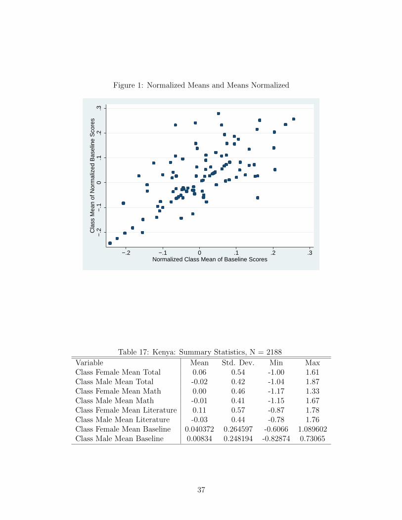
Figure 1: Normalized Means and Means Normalized
−.2
−.1
0.1
.2.3
Cla
ss M
ean
of N
orm
aliz
ed B
asel
ine
Sco
res
−.2 −.1 0 .1 .2 .3Normalized Class Mean of Baseline Scores
Table 17: Kenya: Summary Statistics, N = 2188
Variable Mean Std. Dev. Min MaxClass Female Mean Total 0.06 0.54 -1.00 1.61Class Male Mean Total -0.02 0.42 -1.04 1.87Class Female Mean Math 0.00 0.46 -1.17 1.33Class Male Mean Math -0.01 0.41 -1.15 1.67Class Female Mean Literature 0.11 0.57 -0.87 1.78Class Male Mean Literature -0.03 0.44 -0.78 1.76Class Female Mean Baseline 0.040372 0.264597 -0.6066 1.089602Class Male Mean Baseline 0.00834 0.248194 -0.82874 0.73065
37

significant positive relationship with current scores, as well as that students of new ETP
hires tend to perform better. Notably, the regressions without instruments indicate that
peer effects primarily exist between female students. Furthermore, these female-to-female
peer effects are quite large: a one standard deviation increase in the average score of female
classmates yields a .13 standard deviation increase in the score of female students. This is a
much larger effect than is present in Tables 14, 15, and 16.15
Importantly, this result is not robust to the application of two-stage least squares. While
the coefficient is still positive and very large in the total score and math score regressions,
its standard errors are too large for inference. Therefore, it is unclear whether the apparent
female-to-female effects are truly peer effects or the result of something else—e.g. the exis-
tence of some teachers who are able to more effectively teach math to females. Either result
would be very fascinating, and this question certainly warrants further investigation. In the
future, I hope to continue this line of analysis with larger datasets to determine whether
peer effects are truly a primarily female-to-female phenomenon or whether other factors are
biasing the coefficients in the regression without instruments.
15It is possible that women are the sole drivers of peer effects and that Tables 14, 15, and 16 show smallereffects because they are diluted by males.
38
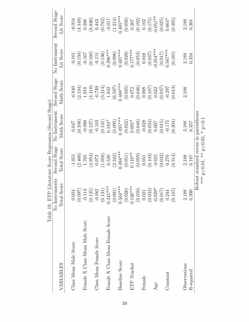
Tab
le18
:E
TP
Lit
erat
ure
Sco
reR
egre
ssio
n(S
econ
dSta
ge)
No
Inst
rum
ents
Sec
ond
Sta
geN
oIn
stru
men
tSec
ond
Sta
geN
oIn
stru
men
tSec
ond
Sta
geV
AR
IAB
LE
ST
otal
Sco
reT
otal
Sco
reM
ath
Sco
reM
ath
Sco
reL
itSco
reL
itSco
re
Cla
ssM
ean
Mal
eSco
re0.
024
-1.0
510.
047
-0.8
40-0
.101
-0.9
18(0
.097
)(2
.460
)(0
.108
)(2
.134
)(0
.150
)(4
.349
)F
emal
eX
Cla
ssM
ean
Mal
eSco
re-0
.113
1.76
5-0
.098
1.91
8-0
.167
0.38
6(0
.125
)(4
.954
)(0
.127
)(4
.418
)(0
.160
)(8
.836
)C
lass
Mea
nF
emal
eSco
re-0
.082
0.07
2-0
.103
-0.7
49-0
.151
0.44
3(0
.131
)(1
.058
)(0
.131
)(3
.214
)(0
.136
)(0
.782
)F
emal
eX
Cla
ssM
ean
Fem
ale
Sco
re0.
245*
**0.
539
0.18
3*1.
832
0.29
6***
-0.0
17(0
.091
)(2
.342
)(0
.095
)(6
.597
)(0
.098
)(1
.214
)B
asel
ine
Sco
re0.
504*
**0.
494*
**0.
495*
**0.
488*
**0.
407*
**0.
405*
**(0
.026
)(0
.051
)(0
.022
)(0
.035
)(0
.029
)(0
.056
)E
TP
Tea
cher
0.13
6***
0.11
6**
0.09
1*0.
072
0.17
7***
0.20
7(0
.050
)(0
.059
)(0
.048
)(0
.046
)(0
.053
)(0
.192
)F
emal
e0.
021
0.05
1-0
.028
0.00
80.
049
0.10
2(0
.033
)(0
.103
)(0
.034
)(0
.187
)(0
.037
)(0
.175
)A
ge-0
.029
*-0
.021
0.00
70.
022
-0.0
54**
*-0
.051
**(0
.017
)(0
.032
)(0
.015
)(0
.047
)(0
.017
)(0
.025
)C
onst
ant
0.24
40.
270
-0.1
75-0
.297
0.56
7***
0.66
4*(0
.185
)(0
.314
)(0
.204
)(0
.613
)(0
.165
)(0
.385
)
Obse
rvat
ions
2,18
82,
188
2,18
82,
188
2,18
82,
188
R-s
quar
ed0.
390
0.18
70.
357
0.33
40.
301
Rob
ust
stan
dar
der
rors
inpar
enth
eses
***
p<
0.01
,**
p<
0.05
,*
p<
0.1
39