hessian-laplace feature detector and haar descriptor for image
TRANSCRIPT
Hessian-Laplace Feature Detector and HaarDescriptor for Image Matching
by
Akshay Bhatia
Thesis submitted to the
Faculty of Graduate and Postdoctoral Studies
In partial fulfillment of the requirements
For the M.A.Sc. degree in
Electrical and Computer Engineering
School of Information Technology and Engineering
Faculty of Engineering
University of Ottawa
c© Akshay Bhatia, Ottawa, Canada, 2007

Abstract
In recent years feature matching using invariant features has gained significant im-
portance due to its application in various recognition problems. Such techniques have
enabled us to match images irrespective of various geometric and photometric transfor-
mations between images. The thesis being presented here focusses on developing such a
feature matching technique which can be used to identify corresponding regions in im-
ages. A feature detection approach is proposed, which finds features that are invariant
to image rotation and scaling, and are also robust to illumination changes. A descrip-
tion is computed for each feature using the local neighborhood around it and then acts
as a unique identifier for the feature. These feature identifiers (or feature descriptors)
are then used to identify point to point correspondences between images. A systematic
comparison is made between this feature detector, and others that are described in the
literature.
Later in this work, we apply the feature matching technique developed here to perform
image retrieval for panoramic images. Our objective here is to retrieve a panoramic image
similar to a query image from a database. We show how such a retrieval task can be
performed by giving results for both indoor and outdoor sequences.
ii

Acknowledgements
First and foremost, I would like to express my heartfelt gratitude towards my super-
visor Dr. Robert Laganiere for giving me the opportunity to work under him. Without
his guidance and constant motivation, this work would not have been possible.
I am grateful to my co-supervisor Dr. Gerhard Roth for his advice and valuable
feedback at every stage of this thesis and his review of this document.
I am also thankful to Dr. Eric Dubois, Dr. Mark Fiala and other NAVIRE group
members for their helpful suggestions during this research.
I would like to thank my colleagues at the VIVA Lab for the great ambiance during
work and especially Florian Kangni with whom I had many useful discussions.
Last but not the least, a special thanks to my family for providing constant support
and encouragement throughout this work.
iii

Contents
1 Introduction 1
1.1 Problem Definition . . . . . . . . . . . . . . . . . . . . . . . . . . . . . . 2
1.2 Contributions . . . . . . . . . . . . . . . . . . . . . . . . . . . . . . . . . 5
1.3 Overview . . . . . . . . . . . . . . . . . . . . . . . . . . . . . . . . . . . . 5
2 Concept of Features and Scale 7
2.1 Selection Criteria for Features . . . . . . . . . . . . . . . . . . . . . . . . 8
2.2 Overview of Corner Detectors . . . . . . . . . . . . . . . . . . . . . . . . 9
2.3 Scale-Space Theory . . . . . . . . . . . . . . . . . . . . . . . . . . . . . . 11
2.3.1 Pyramid Representation . . . . . . . . . . . . . . . . . . . . . . . 12
2.3.2 Scale-Space Representation . . . . . . . . . . . . . . . . . . . . . 13
2.3.3 Hybrid Multi-Scale Representation . . . . . . . . . . . . . . . . . 19
2.4 Scale-Space Derivatives . . . . . . . . . . . . . . . . . . . . . . . . . . . . 19
2.5 Need for Normalization . . . . . . . . . . . . . . . . . . . . . . . . . . . . 21
2.6 Automatic Scale Selection . . . . . . . . . . . . . . . . . . . . . . . . . . 22
2.6.1 Gamma Normalization . . . . . . . . . . . . . . . . . . . . . . . . 23
3 Scale Invariant Features 26
3.1 Related Work . . . . . . . . . . . . . . . . . . . . . . . . . . . . . . . . . 27
3.2 Scale Interpolated Hessian-Laplace Detector . . . . . . . . . . . . . . . . 30
3.2.1 Hessian Matrix . . . . . . . . . . . . . . . . . . . . . . . . . . . . 31
3.2.2 Scale Selection . . . . . . . . . . . . . . . . . . . . . . . . . . . . 32
3.2.3 Keypoint Localization . . . . . . . . . . . . . . . . . . . . . . . . 34
3.2.4 Assigning Orientation to Points . . . . . . . . . . . . . . . . . . . 36
3.2.5 Scale Interpolated Hessian-Laplace and Hessian-Laplace . . . . . . 37
3.3 Repeatability Criterion . . . . . . . . . . . . . . . . . . . . . . . . . . . . 39
3.3.1 Repeatability Tests . . . . . . . . . . . . . . . . . . . . . . . . . . 41
vi

3.3.2 Scaling and Rotation Dataset . . . . . . . . . . . . . . . . . . . . 42
3.3.3 Illumination Change Dataset . . . . . . . . . . . . . . . . . . . . . 46
4 Feature Descriptors for Matching 50
4.1 Related Work . . . . . . . . . . . . . . . . . . . . . . . . . . . . . . . . . 51
4.2 SIFT Descriptor . . . . . . . . . . . . . . . . . . . . . . . . . . . . . . . . 53
4.3 PCA-SIFT Descriptor . . . . . . . . . . . . . . . . . . . . . . . . . . . . 55
4.4 Wavelet Descriptors . . . . . . . . . . . . . . . . . . . . . . . . . . . . . . 57
4.4.1 Haar Descriptor Computation . . . . . . . . . . . . . . . . . . . . 61
4.5 Similarity Measures . . . . . . . . . . . . . . . . . . . . . . . . . . . . . . 62
5 Image Matching and Retrieval 64
5.1 Evaluation Metrics . . . . . . . . . . . . . . . . . . . . . . . . . . . . . . 65
5.2 Different Matching Configurations . . . . . . . . . . . . . . . . . . . . . . 67
5.3 Results for Image Matching . . . . . . . . . . . . . . . . . . . . . . . . . 68
5.3.1 Scaling and Rotation Dataset . . . . . . . . . . . . . . . . . . . . 69
5.3.2 Illumination Change Dataset . . . . . . . . . . . . . . . . . . . . . 75
5.4 Image Retrieval . . . . . . . . . . . . . . . . . . . . . . . . . . . . . . . . 80
5.5 Results . . . . . . . . . . . . . . . . . . . . . . . . . . . . . . . . . . . . . 83
5.5.1 VIVA Lab Sequence . . . . . . . . . . . . . . . . . . . . . . . . . 84
5.5.2 MacDonald Sequence . . . . . . . . . . . . . . . . . . . . . . . . . 90
5.6 Issues with Matching Panoramic Images . . . . . . . . . . . . . . . . . . 93
6 Conclusion 95
6.1 Feature Detectors . . . . . . . . . . . . . . . . . . . . . . . . . . . . . . . 95
6.2 Feature Descriptors . . . . . . . . . . . . . . . . . . . . . . . . . . . . . . 96
6.3 Matching Strategies . . . . . . . . . . . . . . . . . . . . . . . . . . . . . . 97
6.4 Image Retrieval . . . . . . . . . . . . . . . . . . . . . . . . . . . . . . . . 97
6.5 Future Work . . . . . . . . . . . . . . . . . . . . . . . . . . . . . . . . . . 98
A Additional Image Matching Results 99
B Cubic Panoramic Images 103
C Homography 106
C.1 Computing Homography for Calibrated Cameras . . . . . . . . . . . . . . 107
C.1.1 Homography for Image Scaling . . . . . . . . . . . . . . . . . . . 109
vii

C.1.2 Homography for Image Rotation . . . . . . . . . . . . . . . . . . . 110
C.2 Computing Homography for Uncalibrated Cameras . . . . . . . . . . . . 110
D Cubic Panoramic Images for Image Retrieval 112
Bibliography 117
viii

List of Tables
2.1 γ values used to select scales for different types of features . . . . . . . . 25
5.1 Time taken to compute different descriptors. . . . . . . . . . . . . . . . . 75
5.2 Time taken to perform image retrieval for different descriptors. . . . . . . 87
ix
List of Figures
1.1 Feature points . . . . . . . . . . . . . . . . . . . . . . . . . . . . . . . . . 3
1.2 Virtual representation of a real world environment . . . . . . . . . . . . . 4
2.1 Example of a corner point in an image . . . . . . . . . . . . . . . . . . . 8
2.2 Multi-Scale Pyramid Representation . . . . . . . . . . . . . . . . . . . . 13
2.3 Pyramid representation of an image . . . . . . . . . . . . . . . . . . . . . 14
2.4 Scale-Space Representation . . . . . . . . . . . . . . . . . . . . . . . . . 15
2.5 Gaussian images for different levels of the scale-space representation . . . 18
2.6 Hybrid Multi-Scale Representation using Oversampled Pyramids . . . . . 20
2.7 Characteristic scale for image structures . . . . . . . . . . . . . . . . . . 23
3.1 3D extrema in a scale-space representation . . . . . . . . . . . . . . . . . 27
3.2 Points detected at different scale levels using the Hessian matrix . . . . . 33
3.3 Illustration of shape distortion for Hessian points . . . . . . . . . . . . . 34
3.4 Characteristic scale for scaled images . . . . . . . . . . . . . . . . . . . . 35
3.5 Example of a 72 bin orientation histogram for an image patch . . . . . . 38
3.6 Scaling and Rotation Image Dataset . . . . . . . . . . . . . . . . . . . . 43
3.7 Repeatability results with and without localization for an image pair . . 44
3.8 Comparison of different feature detectors for scaling and rotation dataset 45
3.9 Comparison of different feature detectors for an image pair . . . . . . . . 45
3.10 Illumination Change Image Dataset . . . . . . . . . . . . . . . . . . . . 47
3.11 Comparison of different feature detectors for illumination change dataset 48
3.12 Comparison of different feature detectors for an image pair . . . . . . . . 49
4.1 Orientation Histograms for a gradient patch over a 4x4 region . . . . . . 54
4.2 Illustration of trilinear interpolation . . . . . . . . . . . . . . . . . . . . . 55
4.3 Haar basis functions . . . . . . . . . . . . . . . . . . . . . . . . . . . . . 58
4.4 Non-standard decomposition method of wavelet transform . . . . . . . . 60
x
5.1 Evaluation of Haar descriptors for scaling and rotation dataset . . . . . . 70
5.2 Recall vs 1-Precision graphs for different Haar descriptors . . . . . . . . . 70
5.3 Results for different matching strategies . . . . . . . . . . . . . . . . . . . 72
5.4 Recall vs 1-Precision graphs for different matching strategies . . . . . . . 73
5.5 Evaluation of Haar descriptors for illumination change dataset . . . . . . 76
5.6 Recall vs 1-Precision graphs for different Haar descriptors . . . . . . . . . 77
5.7 Results for different matching strategies . . . . . . . . . . . . . . . . . . . 78
5.8 Recall vs 1-Precision graphs for different matching strategies . . . . . . . 79
5.9 Illustration of the image retrieval problem for panoramic images. . . . . 82
5.10 Cubic Panoramic Image, labels indicate the six sides of the cube image . 83
5.11 Sequence Map for Viva Lab Sequence . . . . . . . . . . . . . . . . . . . . 84
5.12 Image Retrieval results for cube images . . . . . . . . . . . . . . . . . . . 86
5.13 Spatial arrangement of matched cubes . . . . . . . . . . . . . . . . . . . 87
5.14 Corresponding faces for matched cube images for query image 24 . . . . . 88
5.15 Corresponding faces for matched cube images for query image 43 . . . . . 89
5.16 Sequence Map for MacDonald Sequence . . . . . . . . . . . . . . . . . . . 91
5.17 Matches obtained between images from sequence 1 and sequence 2 . . . . 92
A.1 Recall vs 1-Precision graphs for different matching strategies . . . . . . . 100
A.2 Recall vs 1-Precision graphs for different matching strategies . . . . . . . 101
A.3 Recall vs 1-Precision graphs for different matching strategies . . . . . . . 102
B.1 Ladybug camera . . . . . . . . . . . . . . . . . . . . . . . . . . . . . . . 103
B.2 Image captured using the Ladybug camera . . . . . . . . . . . . . . . . . 104
B.3 Cubic panoramic image . . . . . . . . . . . . . . . . . . . . . . . . . . . . 105
C.1 Projective transformation for images taken from the same camera center 107
C.2 Projective transformation between two images due to a plane . . . . . . 108
C.3 The pinhole camera model . . . . . . . . . . . . . . . . . . . . . . . . . 109
D.1 Indoor Cubic Panoramic Sequence : VIVA Lab Sequence . . . . . . . . . 113
D.2 Indoor Cubic Panoramic Sequence : VIVA Lab Sequence . . . . . . . . . 114
D.3 Outdoor Cubic Panoramic Sequence : MacDonald Sequence . . . . . . . 115
D.4 Outdoor Cubic Panoramic Sequence : MacDonald Sequence . . . . . . . 116
xi

Chapter 1
Introduction
Computer vision is a discipline of artificial intelligence which focuses on providing com-
puters with the ability to perceive the world as humans would see it. This ability to
mimic human perception constitutes an important step in designing systems which can
perform intelligent tasks.
The real world around us is rich in visual information and interpreting the vast
amount of data can be a challenging process. Vision based systems rely on extracting
information from the images captured in order to carry out a certain task. The type of
information extracted and its analysis depends upon the application to be performed.
More often than not, the ultimate goal is to use this information to gain an understanding
of different objects present in the environment along with their physical and geometrical
attributes.
In the diverse field of vision, recognition is one of the most important problems. It
can be described as the process of perceiving or observing something which is known
a priori. Usually, this a priori information is an object or a pattern or some kind of
activity whose presence we are trying to ascertain. Thus, recognition can be thought of
as an identification process where the description of a certain object is compared to the
reference data to affirm its presence.
Recognition can be classified into numerous sub-fields depending upon the context
in which it is used. One of the frequently used contexts is objects where the goal is to
identify the presence of specific objects or a class of objects along with their locations in
the scene. Apart from objects, recognition is also used in identification of a wide variety
of other patterns like textures, characters, fingerprints and faces just to name a few. It
also forms an important part of applications like content based image retrieval where the
1
2
objective is to find an image similar to a given query image.
A common step in most recognition algorithms requires representing image content
in terms of features. These features which represent specific patterns present in the
image can be used to identify corresponding structures between images. In the past,
most algorithms have relied on detecting low level features like edges, groups of edges,
contours, interest points in order to perform recognition. Although these features work
well for certain applications, their performance degrades considerably in the presence
of background clutter and occlusions. In addition, the ability to detect features which
correspond to the same physical point or group of points significantly reduces when
images are captured from different viewpoints.
In the last decade, a lot of research has been done to study the properties of invariant
features. Invariant features is a generic term used to describe features which result from
a combination of two things; invariant region or feature detectors which detect features
like corners, blobs invariant to scale and affine changes in the image and invariant feature
descriptors which generate a description for a feature which is invariant to geometric and
photometric transformations. The rapid development in the domain of invariant features
has led to a significant improvement in the performance of recognition algorithms. In
the context of this thesis, we study the properties of such invariant features and explore
their applicability to the problem of image retrieval.
1.1 Problem Definition
The thesis being presented here focuses on two main objectives. The primary objective
of this research is to develop a robust, efficient feature matching strategy which can be
used to find correspondences between images. The emphasis here is on developing a
technique which is invariant to geometrical and photometric transformations in images.
In order to find correspondences using invariant features, a two stage approach is
adopted. In the first stage, feature points are detected which are distinctive and robust
to changes in image scale and image rotation. We propose a feature detector called Scale
Interpolated Hessian-Laplace to detect feature points. The detector uses the Hessian
matrix to locate points in the image plane and a Laplacian function to compute scale for
those points. A localization step ensures that the location and scale of the points detected
is close to their true location. Figure 1.1 shows the scale invariant points detected using
this detector. The feature points correspond to the center of the circular regions. The
radii of the circular regions have been chosen proportional to the scale of the points (a
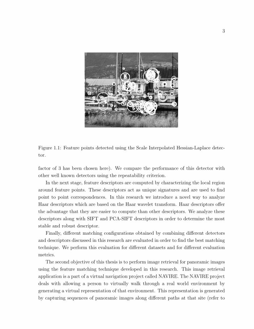
3
Figure 1.1: Feature points detected using the Scale Interpolated Hessian-Laplace detec-
tor.
factor of 3 has been chosen here). We compare the performance of this detector with
other well known detectors using the repeatability criterion.
In the next stage, feature descriptors are computed by characterizing the local region
around feature points. These descriptors act as unique signatures and are used to find
point to point correspondences. In this research we introduce a novel way to analyze
Haar descriptors which are based on the Haar wavelet transform. Haar descriptors offer
the advantage that they are easier to compute than other descriptors. We analyze these
descriptors along with SIFT and PCA-SIFT descriptors in order to determine the most
stable and robust descriptor.
Finally, different matching configurations obtained by combining different detectors
and descriptors discussed in this research are evaluated in order to find the best matching
technique. We perform this evaluation for different datasets and for different evaluation
metrics.
The second objective of this thesis is to perform image retrieval for panoramic images
using the feature matching technique developed in this research. This image retrieval
application is a part of a virtual navigation project called NAVIRE. The NAVIRE project
deals with allowing a person to virtually walk through a real world environment by
generating a virtual representation of that environment. This representation is generated
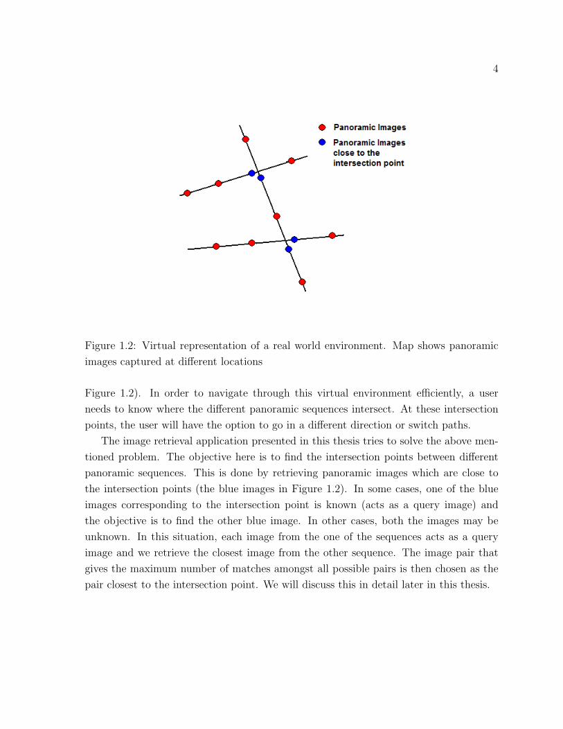
by capturing sequences of panoramic images along different paths at that site (refer to
4
Figure 1.2: Virtual representation of a real world environment. Map shows panoramic
images captured at different locations
Figure 1.2). In order to navigate through this virtual environment efficiently, a user
needs to know where the different panoramic sequences intersect. At these intersection
points, the user will have the option to go in a different direction or switch paths.
The image retrieval application presented in this thesis tries to solve the above men-
tioned problem. The objective here is to find the intersection points between different
panoramic sequences. This is done by retrieving panoramic images which are close to
the intersection points (the blue images in Figure 1.2). In some cases, one of the blue
images corresponding to the intersection point is known (acts as a query image) and
the objective is to find the other blue image. In other cases, both the images may be
unknown. In this situation, each image from the one of the sequences acts as a query
image and we retrieve the closest image from the other sequence. The image pair that
gives the maximum number of matches amongst all possible pairs is then chosen as the
pair closest to the intersection point. We will discuss this in detail later in this thesis.

5
1.2 Contributions
In this research, we propose a scale invariant feature detector called the Scale Interpolated
Hessian-Laplace for detecting feature points. The detector is used to detect points which
are invariant to image scale and rotation. We compare the performance of this detector
with other well known detectors for different image datasets.
This research introduces a novel method to analyze and apply Haar descriptors which
are derived using the Haar wavelet transform. These descriptors offer the advantage that
they are computationally less expensive to compute and smaller in size when compared
to other descriptors. We have evaluated different configurations of Haar descriptors in
this research and compared them with other descriptors.
The different detectors and descriptors studied in this research have been combined
to generate different matching strategies. We evaluate these matching strategies in order
to find the most optimal matching technique. We have carried out these evaluation tests
for different types of sequences using different evaluation metrics.
In the latter part of this thesis, the applicability of the matching technique developed
in this research has been explored in the context of image retrieval for panoramic images.
Here we are interested in identifying images which are close to the intersection points
between different panoramic sequences. We show how the intersection points between
different image sequences can be experimentally determined by using the number of
matches. We carry out these tests using different descriptors for both indoor and outdoor
sequences.
1.3 Overview
This section describes the organization of this thesis.
Chapter 2 describes the concept of features and discusses some of the important
feature detectors, that have been proposed through the course of literature. We then
present the concept of scale-space theory and examine different ways of constructing a
multi-scale representation for an image. The importance of normalization for detecting
the correct scale for a point is also discussed. We also review the concept of automatic
scale selection where the goal is to select the appropriate scale for analyzing an image
structure automatically.
In Chapter 3 we discuss some of the scale invariant feature detectors that are relevant
in context of this research and carry out a comparative evaluation of them. We discuss
6
various important issues that are important for detecting good stable keypoints. We also
talk about a method for estimating orientation for feature points which is used to make
the descriptor of a point invariant to image rotation.
Chapter 4 introduces feature descriptors which are used to represent local regions
around feature points. We describe the formulation of well known descriptors namely
SIFT, PCA-SIFT along with a discussion on descriptors based on Haar wavelet transform.
Different similarity measures used to match descriptors have also been discussed.
Chapter 5 gives the matching results for different image datasets. We evaluate the
performance of different detectors when combined with different descriptors in order
to identify the most robust matching technique. The performance evaluation process
has been performed for different evaluation metrics. Later we discuss the problem of
image retrieval for panoramic images and show how retrieval can be performed using the
matching strategy developed in this research.
Finally, in Chapter 6 we give a summary of the work done and indicate some possible
directions for future research.
Chapter 2
Concept of Features and Scale
Given an image of a scene, a fundamental step in vision based applications is extracting
information about the image content which can act as a representation to complete the
task at hand. The information we are interested in relates to image regions which exhibit
certain properties or some specific patterns. These patterns could be edges, blobs1,
contours of objects, different kinds of junctions and many more things. The collection
of all these image patterns are labelled as image features or simply features. Such types
of features have been used in a wide range of applications like image matching, object
recognition, structure from motion, texture classification just to name a few.
Amongst all the different types of features proposed in the literature, the point based
features are the ones that are most commonly used in the context of image matching.
Feature points or interest points are characteristic points in the image where the image
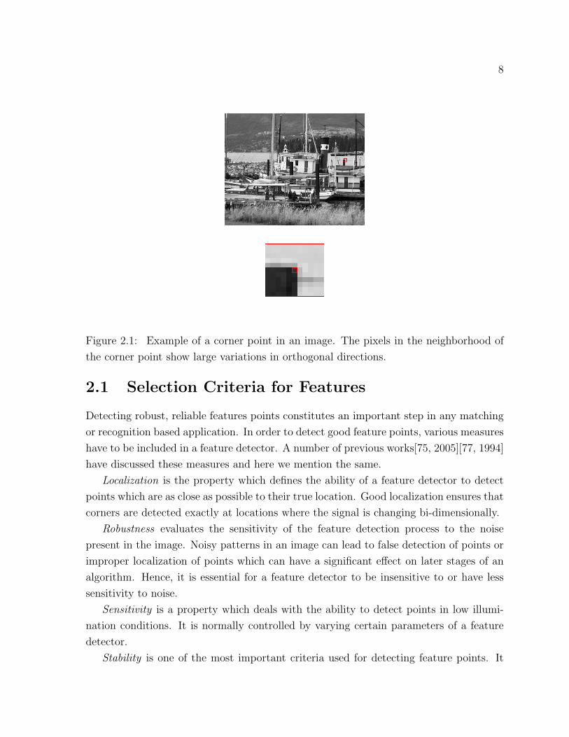
intensity changes in two directions (refer to Figure 2.1). Although, feature points and
interest points is a general term which can be used to describe corners and various types
of junctions, here these terms will implicitly refer to a corner point or a blob.
In the literature, a large number of detectors have been proposed to detect point based
features. In this chapter we give a brief overview of some of the important detectors.
We also review some of the salient properties that the detectors should incorporate so
as to detect points reliably. The next part of the chapter deals with the concept of
multi-scale image representation and scale-space theory. The concept of scale is crucial
for interpreting the multi-scale nature of real world data and for finding corresponding
points across images which have been represented at different scales.
1Blobs are bright areas surrounded by dark pixels or vice versa
7
8
Figure 2.1: Example of a corner point in an image. The pixels in the neighborhood of
the corner point show large variations in orthogonal directions.
2.1 Selection Criteria for Features
Detecting robust, reliable features points constitutes an important step in any matching
or recognition based application. In order to detect good feature points, various measures
have to be included in a feature detector. A number of previous works[75, 2005][77, 1994]
have discussed these measures and here we mention the same.
Localization is the property which defines the ability of a feature detector to detect
points which are as close as possible to their true location. Good localization ensures that
corners are detected exactly at locations where the signal is changing bi-dimensionally.
Robustness evaluates the sensitivity of the feature detection process to the noise
present in the image. Noisy patterns in an image can lead to false detection of points or
improper localization of points which can have a significant effect on later stages of an
algorithm. Hence, it is essential for a feature detector to be insensitive to or have less
sensitivity to noise.
Sensitivity is a property which deals with the ability to detect points in low illumi-
nation conditions. It is normally controlled by varying certain parameters of a feature
detector.
Stability is one of the most important criteria used for detecting feature points. It

9
defines the ability of a detector to extract feature points at the same location in an
image, irrespective of any geometrical or photometric transformation that the image may
undergo. Stability is usually evaluated using the repeatability measure which computes
the number of repeated points between two images. A pair of points detected between two
images is termed repeatable if both the points originate from the same image structure
(i.e to say that both points are the projection of the same 3D point in space). This
number of repeated points directly affects the number of correspondences that can be
found between images. Hence, it is essential for a feature detector to have good stability.
We discuss this in more detail in the next chapter when we explain the repeatability
criterion used to evaluate feature detectors.
Complexity defines the speed at which a detector can detect feature points in an
image. Although, the speed varies depending upon individual implementations, it is
always better if the number of operations required to find features are kept as low as
possible.
It is difficult for a feature detector to satisfy all these conditions simultaneously.
Hence, depending upon the application, more importance is given to some criteria than
others.
2.2 Overview of Corner Detectors
Extracting feature points in an image involves checking for image intensity variations
using different derivative operators. In this section we give an overview of some of the
important methods that have used different order of derivatives and other operators for
extracting feature points.
One of the first interest point detectors was developed by Moravec[59, 1977]. The
detector was based on measuring intensity changes in a local window around a point
in different directions. For each pixel in the image, four sums were computed for four
directions; namely horizontal, vertical and two diagonals, using sum of squared differ-
ences with the adjacent pixels in a neighborhood. A variance measure calculated as the
minimum of these four sums was then used to select interest points in the image.
Beaudet[5, 1978] proposed a detector based on a rotationally invariant measure
termed DET which was computed using the determinant of Hessian matrix. The Hessian
matrix as derived from the second order Taylor series expansion can be used to describe
the local structure around a point. For an image I, the Hessian matrix can be expressed
as
10
H =
[Ixx Ixy
Iyx Iyy
](2.1)
DET = Det(H) = IxxIyy − I2xy (2.2)
where Ixx, Iyy and Ixy are the second order derivatives of image intensity. The extrema
of the DET measure in a local neighborhood was used to detect interest points.
Kitchen and Rosenfeld[35, 1982] introduced a corner detector based on the first and
second order image derivatives. The cornerness measure was defined as
K =IxxIy
2 + IyyIx2 − 2IxyIxIy
Ix2 + Iy
2 (2.3)
This measure was based on product of gradient magnitude and rate of change of
gradient direction along an edge. Before multiplying the gradient magnitude with the
curvature, a non maximum suppression is applied on the magnitude to ensure that it
assumes a maxima along the gradient direction. The local maxima of the measure K was
used to detect corner points.
Deriche and Giraudon[18, 1990] proposed a model for corner detection to improve
the localization accuracy of the Beaudet’s Hessian corner detector. Corners are detected
at two different scale levels using the DET function. The equation of the line connecting
the corner response at the two scales is found, and this is followed by computing the
Laplacian response along the line. The zero crossing of the Laplacian function is then
used to indicate the exact position of the corner.
The Harris detector proposed by Harris and Stephens[26, 1988] is one of most widely
used detectors for finding feature points. It is based on detecting changes in image
intensity around a point using the auto correlation matrix where the matrix is composed
of first order image derivatives. Originally, small filters were used to calculate the image
derivatives. Later on[66, 1998] Gaussian filters were found to be more suitable. The
autocorrelation matrix M can be expressed as
M =
[I2x IxIy
IyIx I2y
](2.4)
Additional smoothing with the Gaussian function is performed to reduce sensitivity
to noise. The eigenvalues of the auto correlation matrix M are used to decide the type
of image pattern present inside the window around a given point. Two large eigenvalues

11
indicate the presence of a corner while one large eigenvalue indicates an edge. The Harris
detector uses a corner response function described in terms of the auto correlation matrix
to detect corners. The corner response function is computed as
R = Det(M)− α(TraceM)2
where R determines the strength of the corner and α is constant chosen to be 0.04.
This function is usually compared against a threshold to give a desired number of corner
points.
Along similar lines as Harris, Noble[62, 1988] proposed a detector using the auto
correlation matrix where the corner function was evaluated as
R = Det(M)/Trace(M) (2.5)
where M is the autocorrelation matrix as defined before.
Amongst all the different corner detectors that have been mentioned here, the Harris
detector and the Hessian detector have been extended to detect scale and affine invariant
features. We will be discussing those detectors in detail in the next chapter. However,
first we discuss the concept of scale for features.
2.3 Scale-Space Theory
The concept of scale plays an important role in the analysis of images. It relates to the
idea of how we perceive objects depending upon the scale of observation. Every object in
the real world has a meaningful interpretation if viewed within a certain range of scales.
An object like a car for example is a meaningful entity if the distance of observation
is measured in meters. In this case it makes little sense to talk about a distance of
observation in kilometers. Similarly in images where our objective is to extract relevant
information by analyzing image structures, the structures can exist for different values
of scale and the amount of information conveyed by the image structure depends on
the scale. This inference about structures in the image has led to the development of
multi-scale image representations where the idea is to represent an image with a family of
images, such that each image conveys information about a different scale of observation.
An important concept for multi-scale data relates to the range of scales within which
an image structure can be analyzed. This range lies between two scales namely the inner
scale and the outer scale. The inner scale for a structure relates to the smallest size

12
of an image patch which can provide sufficient information about the structure in the
patch. This scale is limited by the inner scale of the image which corresponds to the
resolution of the image. The outer scale, on the other hand, depends upon the largest
size of a patch that can be used to describe an image structure. This is in turn limited
by the outer scale of the image, which is the size of the image. The objective in building
a multi-scale representation is to find inner scales for image structures. Thus, the scale
parameter used in a multi-scale representation is the inner scale.
The notion of representing image data in a multi-scale format has to the led to the
development of scale-space theory. Scale-space theory can be described as a theory
developed to study multi-scale representation of images. It has been used to derive
description of structures and relate structures across different scales. In the next few
sections, we discuss some important concepts that have been used to formulate the scale-
space theory, along with properties which are important for detecting scale invariant
features.
2.3.1 Pyramid Representation
The idea of representing images in a multi-scale framework is not new and through the
course of literature, a lot of research has been done to find different ways to generate a
multi-scale representation. Some of the early works done in this area were by Burt and
Adelson[12, 1983] and by Crowley and Parker[14, 1984], where a representation based on
pyramids was proposed. The pyramid was built by performing successive sub-sampling
of finer scale images along with a smoothing operation. The smoothing operation was
incorporated to ensure that aliasing due to sub-sampling did not affect the coarser scale
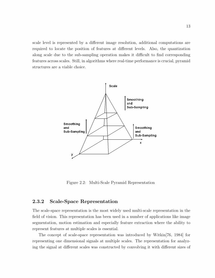
images. Figure 2.2 shows such a multi-scale pyramid.
Since the introduction of pyramid theory, pyramid representations have been fre-
quently used in a wide area of applications. Gaussian pyramids and Difference of Gaus-
sian pyramids have been successfully explored in the fields of data compression, pat-
tern matching and image analysis. Difference of Gaussian pyramids which are built
by subtracting two successive levels of a Gaussian pyramid have been especially useful
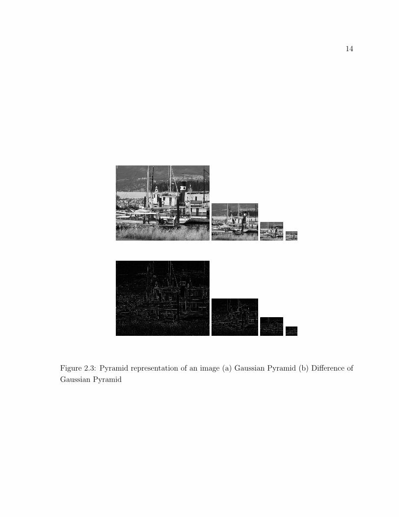
for extracting image features like blobs, edges, ridges etc. Figure 2.3 shows a pyramid
representation constructed for Gaussian and Difference of Gaussian images.
The widespread use of the pyramid representation can be attributed to the fact that
less computation is required as less data has to be processed due to decrease in image
size. However, the pyramid representation also has certain disadvantages. Since each
13
scale level is represented by a different image resolution, additional computations are
required to locate the position of features at different levels. Also, the quantization
along scale due to the sub-sampling operation makes it difficult to find corresponding
features across scales. Still, in algorithms where real-time performance is crucial, pyramid
structures are a viable choice.
Figure 2.2: Multi-Scale Pyramid Representation
2.3.2 Scale-Space Representation
The scale-space representation is the most widely used multi-scale representation in the
field of vision. This representation has been used in a number of applications like image
segmentation, motion estimation and especially feature extraction where the ability to
represent features at multiple scales is essential.
The concept of scale-space representation was introduced by Witkin[76, 1984] for
representing one dimensional signals at multiple scales. The representation for analyz-
ing the signal at different scales was constructed by convolving it with different sizes of
14
Figure 2.3: Pyramid representation of an image (a) Gaussian Pyramid (b) Difference of
Gaussian Pyramid

15
one dimensional kernel. Since the early introduction by Witkin, the scale-space repre-
sentations have been extended to represent two dimensional signals (discrete images) at
multiple scales. Various aspects of these representations have been explored and signif-
icant contributions have been made, which has resulted in a framework which can be
used to describe multi-scale nature of real world data.
The scale-space representation for an image is built by convolving the image with dif-
ferent size of kernels. Unlike the pyramid representation, no sub-sampling is performed,
thus producing a sequence of images which have the same resolution. The scale param-
eter associated with each image is directly related to the σ value of the kernel convolved
with that image. Figure 2.4 shows a scale-space representation. In order to build such
a representation, an important question arises about the choice of convolution operator.
Various studies in the literature have shown that Gaussian kernel is the most optimal
kernel to build such a representation. We now mention some of the important properties
that have led to that conclusion.
Figure 2.4: Scale-Space Representation
Koenderink[36, 1984] proposed the notion of causality for multiple scales which stated
that new image structures should not be created when the scale parameter is increased.
The structures present at higher scales should only be a coarse representation of the
ones at finer scales. He also showed that the scale-space representation should satisfy

16
the diffusion equation, which the Gaussian kernel indeed satisfies.
The property of non-enhancement of local extrema was proposed in conjunction with
the causality principle. The property stated that a maxima or minima present in a scale-
space image should not be enhanced as the scale parameter is increased. This indicates
that extrema of intensity should be suppressed as one moves from a finer scale image
to a coarser scale image. This idea of smoothing out image details with increasing scale
parameter can be accomplished by using a Gaussian kernel.
Another important condition introduced in the same context was that of semi group
structure. The property stated that convolution of an image with two different kernels
should be equivalent to convolution with a single kernel, where σ of the single kernel is
the sum of σ of the two different kernels. Mathematically this can be represented as
I(x, y) ∗ g(x, y, σ) = I(x, y) ∗ g(x, y, σ1) ∗ g(x, y, σ2) (2.6)
where
σ = σ1 + σ2
This condition can be extended for n Gaussian kernels. Thus using this property, nth
level scale-space image can either be computed by performing (n-1) convolutions with
lower scale images or by a direct convolution with the base image. Various other ways
of generating this image are also possible. Other properties that have been mentioned
in this context are linearity, spatial shift invariance, isotropy, scale invariance, rotation
invariance. A detailed description of these properties can been found in many papers in
the literature by Lindeberg[41, 1994][40, 1994], Florack et al.[24, 1992], Koenderink[36,
1984] and many others.
Besides the properties mentioned before, they are other characteristics of the Gaussian
kernel that make it an ideal choice for performing convolution. One of these characteris-
tics is the separability of the Gaussian kernel. The separability allows the convolution to
be computed using a one dimensional kernel, which results in a faster and more efficient
implementation. Also, in addition to this, the ability to simulate Gaussian filtering using
small binomial filters[15, 2002] can lead to a large speed up in the computation process
with a minimal loss in precision. Hence, all these things lead to the conclusion that
Gaussian kernels are the best choice to generate scale-space representations.

17
Now using Gaussian kernels, the process of generating a scale-space representation
can be mathematically expressed as
Gn(x, y) = g(x, y, σn) ∗ I(x, y) (2.7)
where Gn(x, y) denotes the nth level Gaussian image in the scale-space representation
and g(x, y, σn) is the two dimensional Gaussian kernel given as
g(x, y, σn) =1
2πσ2n
exp−x2+y2
2σ2n (2.8)
σn corresponds to the standard deviation of the kernel at the nth scale
σn = sn−1σ1 (2.9)
where s denotes the scale ratio between adjacent images and σ1 is the standard
deviation of the kernel used to generate the first scale image (base image). Figure 2.5
shows such a representation generated for an image.
The equations mentioned above where a symmetric Gaussian kernel has been used,
is used to describe a linear scale-space representation. This type of representation can
be used to analyze features if the scale changes are same in both the spatial directions.
In cases where the scale changes differently in both the directions, an affine Gaussian
scale-space is used.
The affine Gaussian scale-space is created by convolving the image with affine (non
uniform) kernels of varying sizes. An affine scale-space can be treated as a general case
of linear scale-space. The two dimensional gaussian kernels used to compute an affine
scale-space can be represented as
g(x, Σ) =1
2π√
detΣexp−
xT Σ−1x2 (2.10)
where Σ is the covariance matrix. This representation of a Gaussian kernel is equiv-
alent to its rotationally symmetric representation if the covariance matrix is an identity
matrix multiplied by a factor. Affine scale-space was first explored by Lindeberg and
Garding[44, 1997] to perform shape adaptation so as to reduce distortions due to rota-
tionally symmetric kernels in the context of computing shape cues. This representation
has also been used by Mikolajczyk and Schmid[56, 2004] to detect features points that
are invariant to affine transformation.
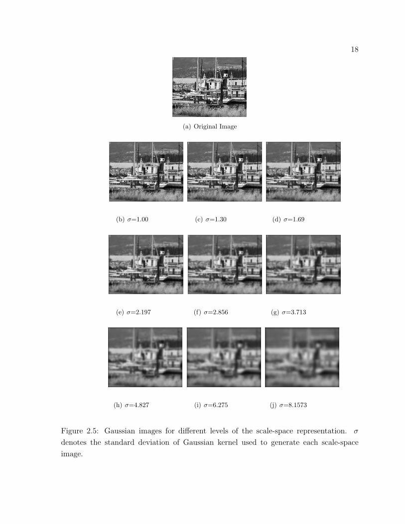
18
(a) Original Image
(b) σ=1.00 (c) σ=1.30 (d) σ=1.69
(e) σ=2.197 (f) σ=2.856 (g) σ=3.713
(h) σ=4.827 (i) σ=6.275 (j) σ=8.1573
Figure 2.5: Gaussian images for different levels of the scale-space representation. σ
denotes the standard deviation of Gaussian kernel used to generate each scale-space
image.
19
In the context of this research, since we are concerned with scale invariant features,
we will focus on the linear scale-space representation. However, almost all the concepts
mentioned here will also be applicable to an affine Gaussian scale-space.
2.3.3 Hybrid Multi-Scale Representation
Another type of multi-scale representation that has been developed recently is the hybrid
representation[43, 2003]. The hybrid representation as the name suggests, is a fusion of
the pyramid representation and the scale-space representation. Representations based
on pyramids have the advantage of reducing image resolution which can be beneficial
for fast processing needs. However, it is difficult to match image structures in pyramids
across different scales. Scale-space representations on the other hand provide a smooth
transition between different scales. However, for coarse scale values there is a lot of re-
dundant information present. The hybrid representation tries to combine the advantages
of these two approaches so as to develop a framework which can be used in real time
without losing accuracy.
A hybrid representation can be build in two ways: the Sub-Sampled Scale-Space Repre-
sentation and the Oversampled Pyramid Representation as mentioned by Niemenmaa[61,
2001]. The Sub-Sampled Scale-Space Representation is generated similar to a scale-
space representation, with sub-sampling of the image performed at certain stages. The
frequency of sub-sampling is decided by the scale factor and the distance between pix-
els. The Oversampled Pyramid Representation on the other hand is constructed similar
to a Pyramid Representation, but with the smoothing operation divided into several
smoothing steps. Separation of the smoothing operation results in a more continuous
scale than the original pyramid representation. Figure 2.6 shows an Oversampled Pyra-
mid Representation. This latter representation has been investigated by Lindeberg and
Bretzner[43, 2003] and was used in their work to test its efficiency for blob detection. A
similar representation using Difference of Gaussian has been used by Lowe[47, 2004] for
extracting scale invariant feature points.
2.4 Scale-Space Derivatives
One of the important applications of multi-scale image representations is in the context
of feature detection. As mentioned previously while discussing feature detectors, finding
features requires computing image derivatives. In the context of scale-space representa-

20
Figure 2.6: Hybrid Multi-Scale Representation using Oversampled Pyramids

21
tion this indicates that we have to build a representation which consists of derivatives of
scale-space images.
The task of computing a derivative scale-space image can be accomplished in a number
of ways. We can either compute the derivative of the image first and then convolve it
with Gaussian
L(x; σ) =∂
∂xI(x) ∗G(x; σ) (2.11)
or convolve the image with derivative of a Gaussian function.
L(x; σ) =∂
∂xG(x; σ) ∗ I(x) (2.12)
Finally, we can also directly compute the derivative for a scale-space image
L(x; σ) =∂
∂x(I(x) ∗G(x; σ)) (2.13)
Similar rules apply for higher order derivatives. All the above equations can be
also be computed in the Fourier domain. These operations are equivalent due to the
commutative property of the derivative and convolution operator.
2.5 Need for Normalization
In a scale-space representation, as we move from finer scales to coarser scales, the amount
of smoothing provided by the Gaussian function increases. This smoothing reduces the
high frequency information in the image, thus causing the amplitudes of spatial deriva-
tives to decrease with an increase in scale. In many applications analyzing derivatives
at various scales constitutes an essential step. This is especially true for feature detec-
tion process where selecting a scale for a feature requires comparing spatial derivatives
at different scales. Thus in order to devise a method which permits comparison across
scales, it is necessary to perform normalization with respect to scale.
Let Ln be the nth order derivative of an image at scale σs before normalization and
Dn be the derivative at the same scale after normalization. Then the scale normalized
derivative can be expressed as
Dn(x, y, σs) = σns ∗ Ln(x, y, σs) (2.14)

22
This type of normalization is particularly useful for detecting features like blobs and
corners. Normalization of derivatives also constitutes an essential step in the process of
automatic scale selection, which is discussed in the next section.
2.6 Automatic Scale Selection
A scale-space representation of an image is a family of images where each image corre-
sponds to a particular scale. When analyzing such a representation an important question
that arises is, which is most appropriate scale to represent a feature? Storing the descrip-
tion of a feature at all scales not only requires a lot of storage but significantly increases
the computations required to find the correct correspondence for a feature. This issue
of representing the a feature at its most appropriate scale was extensively investigated
by Lindeberg[42, 1998] and a selection mechanism which automatically selects the best
scale(s) was proposed. Here we discuss that automatic scale selection mechanism.
The basic idea behind the scale selection principle is to select a scale at which the
response of a given function attains a local maxima over scales. This function is usually
composed of a combination of scale normalized derivatives. The scale for a feature at
which the maxima is attained is called the characteristic scale. Since the response of
a function can contain more than once local maxima, a point can have more than one
characteristic scale. Lindeberg proposed to use the scale normalized Laplacian function
for finding the characteristic scale for a feature. The scale normalized Laplacian function
used can be represented as
Laplacian = σ2(Cxx(x, y, σ) + Cyy(x, y, σ)) (2.15)
where Cxx and Cyy are second order derivatives in x and y directions respectively.
Later, Mikolajczyk and Schmid[55, 2001] evaluated various functions for their ability to
detect the correct characteristic scale for feature points and concluded that Laplacian is
indeed the optimal function for scale selection. The characteristic scale in their case was
found by looking for maxima in the absolute response of the Laplacian.
An important condition that the automatic scale selection principle should satisfy
is that if the image is scaled by a factor f , then the characteristic scale at which an
image structure was detected should also be multiplied by the same factor. Figure 2.7
shows an example of this. For the structure in the left image the characteristic scale was
detected at σ=2 which means that rescaling the image by a factor of 2 should result in

23
the characteristic scale being detected at σ=4. This ensures that characteristic scale for
a structure changes in the appropriate fashion with the size of the structure.
(a) σ=2 (b) σ=4
Figure 2.7: σ indicates the characteristic scale for the same image structure detected in
two images. The two images differ by a scale factor of 2
2.6.1 Gamma Normalization
So far the normalization procedure than has been discussed for derivatives assumed the
γ parameter as unity. Now we discuss the more general case of normalization known as
gamma normalization. The choice of the γ factor also plays an important role is deciding
the most suitable scale for features in the process of automatic scale selection.
Again, let Ln be the nth order derivative of an image at scale σs before normalization
and Dn be the derivative at the same scale after normalization. Then the scale normalized
derivative with the γ parameter can be expressed as
Dn(x, y, σs) = σγns ∗ Ln(x, y, σs) (2.16)
The affect of the γ factor on the response of normalized derivatives can be considered
from the following derivation as proposed by Lindeberg[42, 1998].
Consider two images I1 and I2 where I2 is a scaled version of I1 by a factor s. The
relation between these images can thus be given by the following equation
I1(x1) = I2(sx1) (2.17)
Let the scale-space representation of these images be given by L1 and L2. Then we
have

24
L1(x1; σ1) = L2(x2; σ2) (2.18)
where
L1(x1; σ1) = g(x; σ1) ∗ I1(x1) (2.19)
L2(x2; σ2) = g(x; σ2) ∗ I2(x2) (2.20)
and
σ2 = sσ1 x2 = sx1 (2.21)
The nthorder derivative for these images can then be expressed as
L1n(x1; σ1) = snL2n(x2; σ2) (2.22)
Replacing these derivatives with γ normalized derivatives from equation 2.16 yields
D1n(x1; σ1)
σγn1
= sn D2n(x2; σ2)
σγn2
(2.23)
thus giving
D1n(x1; σ1) = sn(1−γ)D2n(x2; σ2) (2.24)
For the factor γ=1 we obtain the condition of perfect scale invariance. For this
condition normalized derivatives will be same for both images. This condition arises
when the function used to compute the maxima over scales is composed of the same order
derivatives (example the Laplacian in equation 2.15). Perfect scale invariance implies that
the response of normalized derivatives is independent of the image resolution.
The case in which γ 6=1 arises when the function used is made up of different order
derivatives. In such a scenario the magnitude of normalized derivatives varies with image
resolution. However, even is such cases, it is possible to locate the local maxima over
scales for a given feature.
The choice of gamma operator can also influence the type of features detected. This
indicates that for any given image structure, there is a finite range of gamma values
within which the local maxima for a structure will be detected i.e. the structure will be
assigned a scale. This property was studied by Majer[49, 2001] and used to detect ridges
25
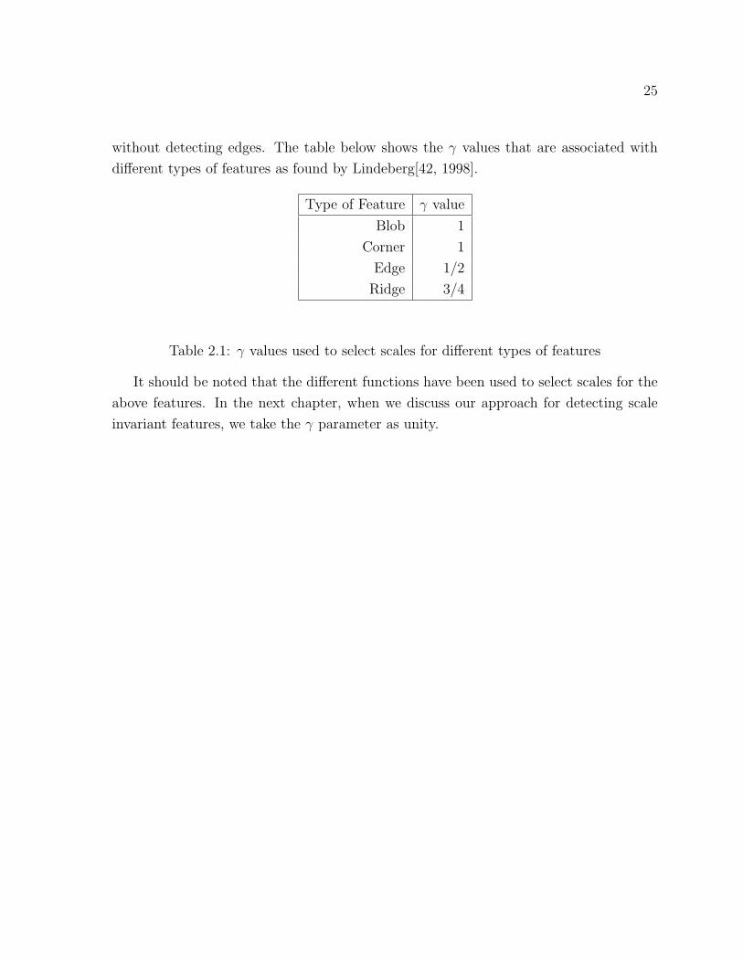
without detecting edges. The table below shows the γ values that are associated with
different types of features as found by Lindeberg[42, 1998].
Type of Feature γ value
Blob 1
Corner 1
Edge 1/2
Ridge 3/4
Table 2.1: γ values used to select scales for different types of features
It should be noted that the different functions have been used to select scales for the
above features. In the next chapter, when we discuss our approach for detecting scale
invariant features, we take the γ parameter as unity.

Chapter 3
Scale Invariant Features
Having discussed the concept of scale in the previous chapter we now explore the do-
main of scale invariant features. These features are extracted using multi-scale image
representations where image points are associated with a scale parameter by searching
for maxima of some function. The scale parameter thus obtained is used to assign a
circular region to each feature point. Hence, unlike ordinary features, scale invariant
features have associated regions. These regions are later used to generate descriptors for
these feature points (discussed in chapter 4) which are eventually used to match feature
points between images. Although these features are scale invariant, the detectors used
to detect these features can also handle small affine transformations.
In the next section we review some of the scale and affine invariant detectors that
have proposed in the literature. We then talk about the Scale Interpolated Hessian-
Laplace detector which has been used in this research to extract scale invariant points,
along with various aspects related to the detection process. We highlight the differences
between this detector and the Hessian-Laplace detector which has been proposed in an
earlier research. In the end of this chapter, we do an evaluation study where we compare
the performance of different detectors using the repeatability measure. The repeatability
measure is used to evaluate the stability of points detected across images (see section
2.1). The repeatability between images directly affects the number of correspondences
that can be found between them. We evaluate the repeatability of different detectors for
different image datasets.
26
27
3.1 Related Work
This section gives an overview of some of the approaches that have been used to design
scale invariant feature detectors.
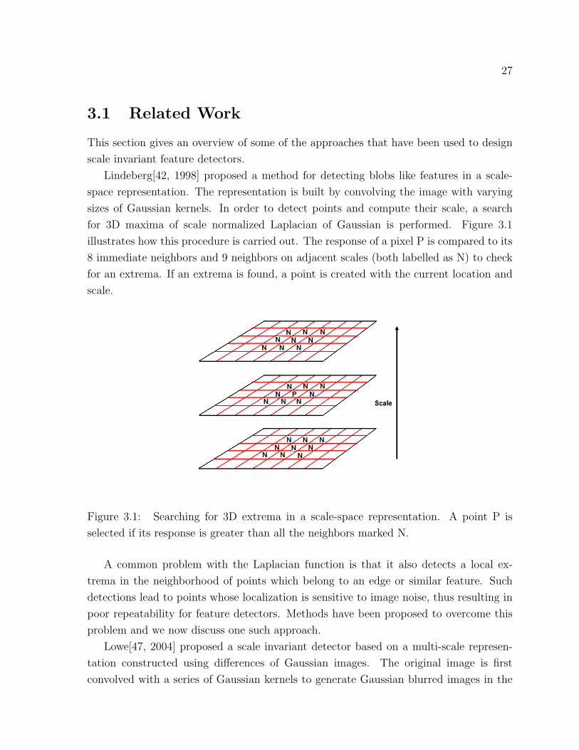
Lindeberg[42, 1998] proposed a method for detecting blobs like features in a scale-
space representation. The representation is built by convolving the image with varying
sizes of Gaussian kernels. In order to detect points and compute their scale, a search
for 3D maxima of scale normalized Laplacian of Gaussian is performed. Figure 3.1
illustrates how this procedure is carried out. The response of a pixel P is compared to its
8 immediate neighbors and 9 neighbors on adjacent scales (both labelled as N) to check
for an extrema. If an extrema is found, a point is created with the current location and
scale.
Figure 3.1: Searching for 3D extrema in a scale-space representation. A point P is
selected if its response is greater than all the neighbors marked N.
A common problem with the Laplacian function is that it also detects a local ex-
trema in the neighborhood of points which belong to an edge or similar feature. Such
detections lead to points whose localization is sensitive to image noise, thus resulting in
poor repeatability for feature detectors. Methods have been proposed to overcome this
problem and we now discuss one such approach.
Lowe[47, 2004] proposed a scale invariant detector based on a multi-scale represen-
tation constructed using differences of Gaussian images. The original image is first
convolved with a series of Gaussian kernels to generate Gaussian blurred images in the
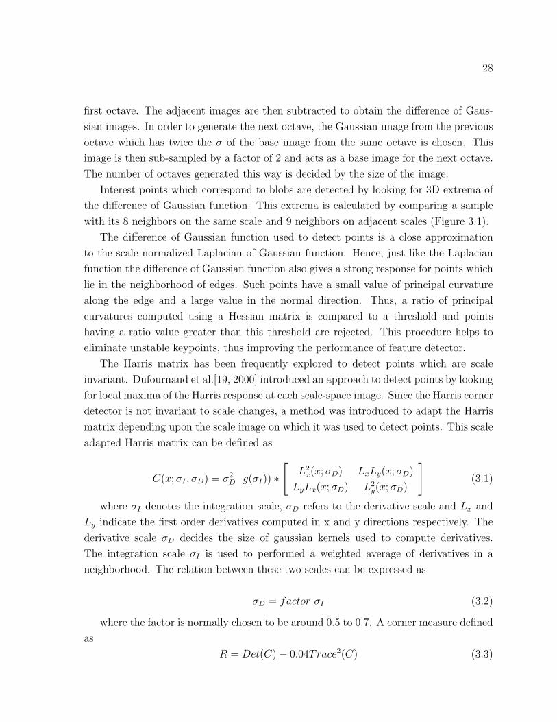
28
first octave. The adjacent images are then subtracted to obtain the difference of Gaus-
sian images. In order to generate the next octave, the Gaussian image from the previous
octave which has twice the σ of the base image from the same octave is chosen. This
image is then sub-sampled by a factor of 2 and acts as a base image for the next octave.
The number of octaves generated this way is decided by the size of the image.
Interest points which correspond to blobs are detected by looking for 3D extrema of
the difference of Gaussian function. This extrema is calculated by comparing a sample
with its 8 neighbors on the same scale and 9 neighbors on adjacent scales (Figure 3.1).
The difference of Gaussian function used to detect points is a close approximation
to the scale normalized Laplacian of Gaussian function. Hence, just like the Laplacian
function the difference of Gaussian function also gives a strong response for points which
lie in the neighborhood of edges. Such points have a small value of principal curvature
along the edge and a large value in the normal direction. Thus, a ratio of principal
curvatures computed using a Hessian matrix is compared to a threshold and points
having a ratio value greater than this threshold are rejected. This procedure helps to
eliminate unstable keypoints, thus improving the performance of feature detector.
The Harris matrix has been frequently explored to detect points which are scale
invariant. Dufournaud et al.[19, 2000] introduced an approach to detect points by looking
for local maxima of the Harris response at each scale-space image. Since the Harris corner
detector is not invariant to scale changes, a method was introduced to adapt the Harris
matrix depending upon the scale image on which it was used to detect points. This scale
adapted Harris matrix can be defined as
C(x; σI , σD) = σ2D g(σI)) ∗
[L2
x(x; σD) LxLy(x; σD)
LyLx(x; σD) L2y(x; σD)
](3.1)
where σI denotes the integration scale, σD refers to the derivative scale and Lx and
Ly indicate the first order derivatives computed in x and y directions respectively. The
derivative scale σD decides the size of gaussian kernels used to compute derivatives.
The integration scale σI is used to performed a weighted average of derivatives in a
neighborhood. The relation between these two scales can be expressed as
σD = factor σI (3.2)
where the factor is normally chosen to be around 0.5 to 0.7. A corner measure defined
as
R = Det(C)− 0.04Trace2(C) (3.3)
29
is used to detect points by looking for maxima of the measure R in a neighborhood.
This procedure was used to detect points for a predefined number of scales where points at
all scales were used to perform matching. Hence no criteria was used to select appropriate
scale(s) for a feature. Later, Mikolajczyk and Schmid[55, 2001] extended the detector by
combining it with the Laplacian function to form the Harris-Laplace detector. For Harris
points computed at different scales, a scale normalized Laplacian response is calculated
over all the scales. The local extrema of this response is then used to select the scale for
a feature.
Kadir and Brady[32, 2001] introduced the concept of Salient Regions which are de-
tected with a two stage approach using the measure of entropy. In the first stage, a
number of descriptors are computed for every pixel in the image for a range of scales.
These descriptors are vectors of gray scale values in a patch which is selected propor-
tional to the value of scale. A probability density function (PDF) estimated from the
descriptors is used to measure the entropy for different levels. The levels at which the
entropy measure attains a local maxima constitute the keypoint’s scales. A weighting
function computed using sum of absolute differences of PDF is also associated with each
maxima scale. These points with their scales form the candidate salient regions. In the
next stage, a saliency metric computed using the entropy and the weighting function is
used to rank the regions where the top few regions are retained.
The detectors that have been presented so far are invariant to scale changes and small
affine changes. A generalization of these detectors are the affine invariant detectors which
are robust to significant affine transformations. We now mention some of these affine
invariant approaches since affine detectors do incorporate scale invariance. However, it
should be noted that for images having large scale differences, scale invariant detectors
perform better than their affine counterparts.
Lindeberg and Garding[44, 1997] proposed a method to find affine features using the
second moment matrix. Given a point at a scale, an iterative method is used where
the second moment matrix using affine kernels adapts the scale and shape of the point’s
neighborhood. The method converges when the difference between second moment ma-
trices in successive iterations is within a threshold. The location of the points remains
unchanged in successive iterations.
An approach based on the same concept was proposed by Mikolajczyk and Schmid[56,
2004]. In the case of the Harris-Affine detector, an iterative method is used to estimate
the new location and scale of the point. The objective here is to use the second moment
matrix for two purposes; to look for local maxima to find the new scale and location and
30
to estimate the shape of the local patch. In order to do so, a shape adaptation matrix
is first computed from the second moment matrix from the previous iteration in order
to normalize the region around a point. The goal is to use a normalized image patch
so that uniform gaussian kernels can estimate the location and scale of a point, rather
than affine kernels. Once the eigenvalues for the second moment matrix computed at the
new location are sufficiently close, the scale is equal in both the directions indicating the
iterative process has converged. A similar approach was also adopted for the Hessian-
Affine detector where the Hessian matrix was used instead of the Harris matrix.
Tuytelaars and Van Gool[72, 1999] proposed a method to extract affine invariant
regions for corner points by using image edges. Two edges are considered for each corner
point where the edges pass through the point. For all the points along the two edges, a
search for an extremum of a function is performed. The distance between the extrema
points and the corner point is then used to describe an invariant parallelogram. In
another approach proposed by the same authors[73, 2000], image intensities are examined
to select points which correspond to extrema of intensity. Given such an extremum in
the image, the rays radiating outward from this point are analyzed by measuring the
response of a given function. The points along those rays where the function reaches an
extremum are then selected to make a closed bounded region. These points correspond
to positions where the change in intensity is significant. Finally, the closed bounded
region is approximated by an ellipse to obtain an invariant region.
Affine Salient Regions[33, 2004] are an extension of the salient regions mentioned
before where instead of using isotropic regions for constructing descriptors at various
scales, anisotropic regions are used. A more extensive review and analysis of various
affine approaches can be found in the article by Mikolajczyk et al.[58, 2005].
3.2 Scale Interpolated Hessian-Laplace Detector
The Hessian-Laplace detector proposed by Mikolajczyk and Schmid[56, 2004] is a scale
invariant detector which is used to detect points which correspond to blobs in an image.
The detector uses the Hessian matrix to locate points in space and the Laplacian function
to compute their scale. In this section we introduce the Scale Interpolated Hessian-
Laplace (SIHL) detector which is based on the Hessian-Laplace detector. We explain
in detail the procedure for detecting Hessian-Laplace points followed by the keypoint
localization step which is essential in order to obtain good keypoints. We also discuss a
method for assigning orientation to a feature point which is used to make the descriptor of

31
feature point invariant to image rotation (Chapter 4). Finally, we highlight the important
differences between the Scale Interpolated Hessian-Laplace approach and the standard
Hessian-Laplace approach.
3.2.1 Hessian Matrix
The Hessian matrix is composed of second order partial derivatives derived from Taylor
series expansion. This matrix has been frequently used to analyze local image structures.
The 2x2 Hessian matrix can be expressed as
H =
[Ixx(x; σD) Ixy(x; σD)
Iyx(x; σD) Iyy(x; σD)
](3.4)
where Ixx, Iyy and Ixy are the second order derivatives computed using Gaussian
kernels of standard deviation σD.
The second order derivatives used in the Hessian matrix can be used to measure the
curvature at a point when the image is treated as an intensity surface. The eigenvectors of
the matrix give the directions for minimum and maximum curvature while the eigenvalues
correspond to the amount of curvature in those directions. Hence, using the Hessian
matrix it is possible to describe the local structure in a neighborhood around a point.
The determinant of the Hessian matrix can be used to detect image structures which
have strong signal variations in two directions. Here we make use of this property of
the Hessian matrix to detect interest points in an image. We first build a scale-space
representation by convolving the image with Gaussians of increasing size. The scale of a
scale-space image is equal to the standard deviation of Gaussian kernel used to generate
that image. The Gaussian kernels are chosen such that successive images differ by a scale
ratio of 1.3. Since we plan to detect points at different scale levels using the Hessian
matrix, the matrix has to be made invariant to scale. Hence a factor σ2D is multiplied
with the Hessian matrix where σD represents the scale of the image. This means that the
determinant computed at each scale level is multiplied by a factor of σ4D. For every image
in the representation, points are extracted by comparing the Hessian determinant value
of a pixel with its adjacent neighbors in a 3x3 neighborhood. If the value at the current
pixel is greater than its neighbors and also above a given threshold, then a feature point
is associated with the current location. Using a threshold helps to eliminate points which
have weak maxima.
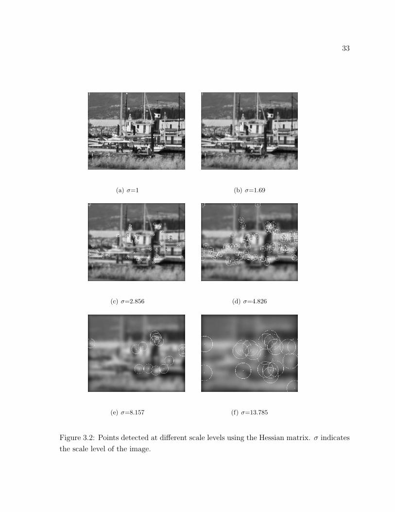
Figure 3.2 shows the Hessian feature points detected at different levels of the scale-

32
space representation. The circular regions around the points are drawn in proportion to
the scale at which points are detected. Here the radius of the circles is equal to 3 times
the scale of the points. An observation that can be made from the points detected at
different scales is that the location of these points changes depending upon the scale at
which they are detected. Figure 3.3 shows a part of an image where the points detected
at all scales have been superimposed on the original image. This drift in the location of
points is due to smoothing performed using rotationally symmetric gaussian kernels.
3.2.2 Scale Selection
Once we have the spatial location of points detected on different levels of the scale-space
representation, the next stage involves computing the proper scale for these points. The
scales where the description of the image points convey the maximum information are
termed as characteristic scales. A number of previous experiments have shown that the
Laplacian function is the most suitable function for detecting the characteristic scale for
an image structure. Hence, here we make use of the Laplacian to find the scale for a
point.
As discussed before in the previous chapter, in order to compare the response of a
function at different scales, normalization of the response with respect to a given scale
has to be performed (see section 2.5). The scale normalized Laplacian function that is
used to select the proper scale can be expressed as
Laplacian(x; σD) = σ2D|Ixx(x; σD) + Iyy(x; σD)| (3.5)
where Ixx and Iyy are second order derivatives. One of the advantages of using the
Hessian matrix is evident here as the Laplacian function can be computed using the trace
of the Hessian matrix.
For a point detected in a scale-space image, its Laplacian is computed over all scales
and the scale for which the Laplacian attains a local maximum is assigned as the char-
acteristic scale. Local maximum here corresponds to response for a given scale being
greater than its adjacent scales and above a given threshold. In some cases the Lapla-
cian function will attain more than one local maximum, and in those cases the point is
assigned more than one characteristic scale. Figure 3.4 shows the same image structure
detected in two images along with the scale normalized trace response for the image
structure. As can be observed from the these images, the trace of the image structure
in the second image attains a local maximum at two scales so this point is assigned
33
(a) σ=1 (b) σ=1.69
(c) σ=2.856 (d) σ=4.826
(e) σ=8.157 (f) σ=13.785
Figure 3.2: Points detected at different scale levels using the Hessian matrix. σ indicates
the scale level of the image.
34
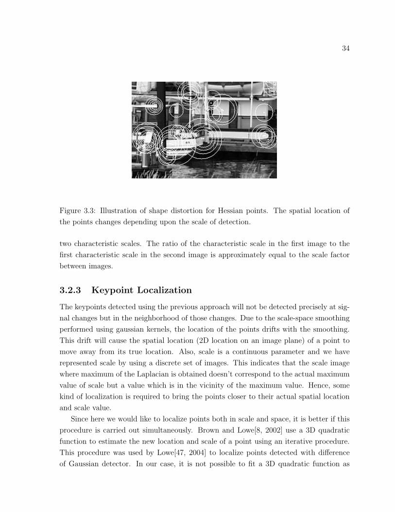
Figure 3.3: Illustration of shape distortion for Hessian points. The spatial location of
the points changes depending upon the scale of detection.
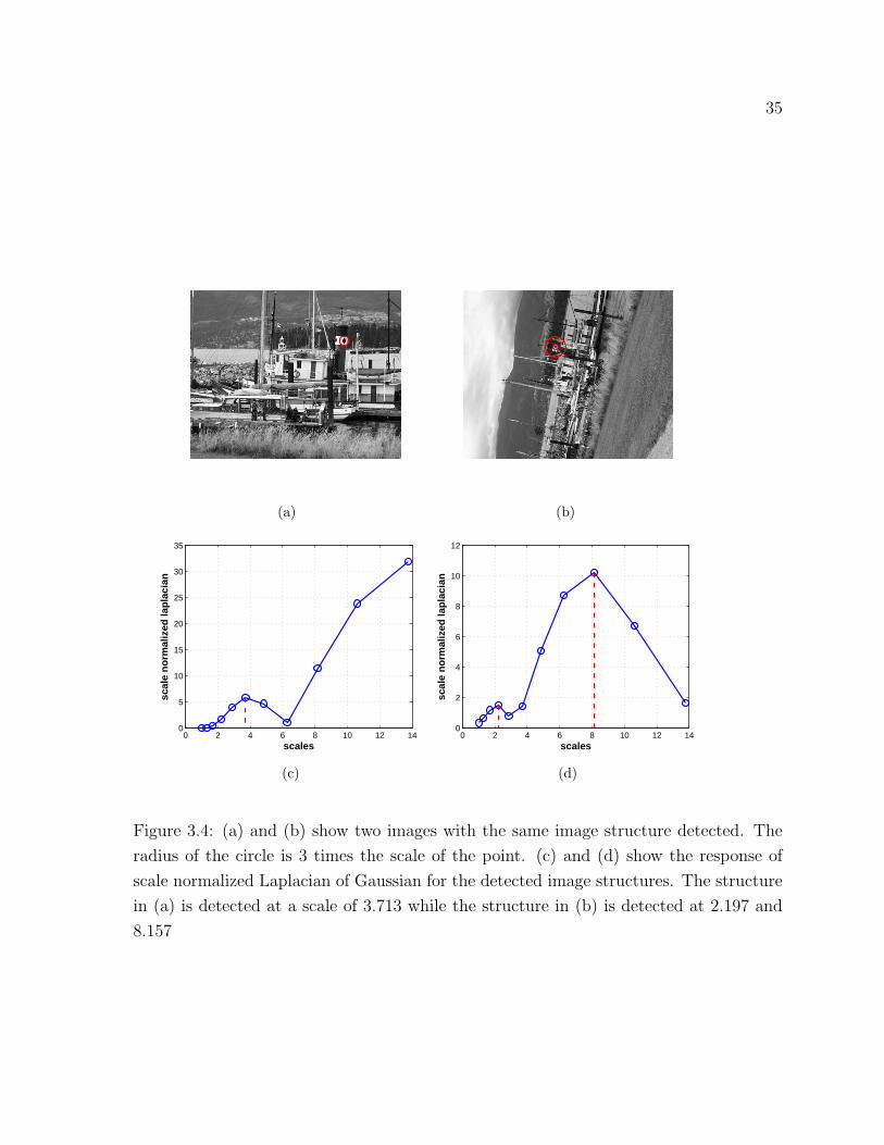
two characteristic scales. The ratio of the characteristic scale in the first image to the
first characteristic scale in the second image is approximately equal to the scale factor
between images.
3.2.3 Keypoint Localization
The keypoints detected using the previous approach will not be detected precisely at sig-
nal changes but in the neighborhood of those changes. Due to the scale-space smoothing
performed using gaussian kernels, the location of the points drifts with the smoothing.
This drift will cause the spatial location (2D location on an image plane) of a point to
move away from its true location. Also, scale is a continuous parameter and we have
represented scale by using a discrete set of images. This indicates that the scale image
where maximum of the Laplacian is obtained doesn’t correspond to the actual maximum
value of scale but a value which is in the vicinity of the maximum value. Hence, some
kind of localization is required to bring the points closer to their actual spatial location
and scale value.
Since here we would like to localize points both in scale and space, it is better if this
procedure is carried out simultaneously. Brown and Lowe[8, 2002] use a 3D quadratic
function to estimate the new location and scale of a point using an iterative procedure.
This procedure was used by Lowe[47, 2004] to localize points detected with difference
of Gaussian detector. In our case, it is not possible to fit a 3D quadratic function as
35
(a) (b)
0 2 4 6 8 10 12 140
5
10
15
20
25
30
35
scales
scal
e n
orm
aliz
ed la
pla
cian
(c)
0 2 4 6 8 10 12 140
2
4
6
8
10
12
scales
scal
e n
orm
aliz
ed la
pla
cian
(d)
Figure 3.4: (a) and (b) show two images with the same image structure detected. The
radius of the circle is 3 times the scale of the point. (c) and (d) show the response of
scale normalized Laplacian of Gaussian for the detected image structures. The structure
in (a) is detected at a scale of 3.713 while the structure in (b) is detected at 2.197 and
8.157
36
two separate functions namely the determinant of Hessian matrix and scale normalized
Laplacian are used to detect points in space and scale respectively. Another possible
approach could be to obtain the new maximum scale for a point and to look for spatial
maxima on that new scale . However, this new maximum scale will lie between two scale
images and fitting a 2D quadratic to find the new location will require the intermediate
scale image which is time consuming. This indicates that performing localization in scale
and space at the same time is not an easy task.
An observation that can be made from a scale-space representation is that for large
scale values the scale difference between successive images is greater (here we are referring
to the scale difference and not the scale ratio which is constant). This causes the error
between the scale of the point and its localized scale to increase for larger scales. This
error in the scale value also affects the computation of orientation and image description
of a point as the these operations require the selection of an image patch around the
point which is proportional to its scale value. Hence, here we focus more on choosing
the correct scale for a point than localizing it in the spatial domain. Given a point at
a scale image s, we fit a parabola between the image s and its adjacent scale images.
The scale for which the parabola attains a maximum is selected as the new scale for the
point. We also compute the sub pixel location of the point using bilinear interpolation in
a 3x3 neighborhood. This interpolation is performed on the scale-space image where the
point was originally detected. Even though the points obtained using this method are
not perfectly localized in space (2D location in the image plane), these points are still
well localized in scale. We show the results for this localization step when we discuss the
repeatability criterion later in this chapter (see section 3.3.2).
3.2.4 Assigning Orientation to Points
Computing orientation for a keypoint is an important step in the invariant feature de-
tection process. This orientation is used to make the keypoint’s description invariant to
changes in image rotation. In the literature, one of the most efficient methods in this
context has been proposed by Lowe[47, 2004]. This approach is based on assigning orien-
tation to a keypoint depending upon the local gradient information in its neighborhood.
In this research, we make use of their method for estimating the dominant orientation.
We start by selecting a patch around the keypoint which is proportional to its scale
and selected from the appropriate scale-space image. The scale-space image is the one
that either corresponds to the scale of the point or is the closest to the scale. The
37
information in the patch is used to compute gradient magnitude and angle at each pixel
location. Using this gradient information, an orientation histogram is generated where
each sample added to the histogram is weighed by a Gaussian function centered at the
keypoint. The histogram uses 72 bins for the 360◦ range (Lowe proposed to use a 36 bin
histogram).
The dominant orientation for a keypoint is obtained by selecting the bin with the
highest peak in the histogram. However, since the bins represent only a range of ori-
entations, a parabola is fit between the selected bin and the adjacent bins to get the
precise value of orientation. Unlike the method proposed by Lowe where some points
are assigned multiple orientations, here we use a single orientation per point. Figure 3.5
shows a patch with its orientation histogram.
3.2.5 Differences between Scale Interpolated Hessian-Laplace
and Hessian-Laplace
Although the Hessian-Laplace (HL) detector (introduced by Mikolajczyk and Schmid[56,
2004]) and the Scale Interpolated Hessian-Laplace (SIHL) detector are based on the same
principle, they differ in a number of aspects. The first important difference between the
two approaches originates from the methods used to localize the feature points. The
HL detector uses an iterative procedure to localize points. Given an initial location and
scale for a point, the maximum of Laplacian is computed again such that the maxima
lies between adjacent scale images. Thus the process requires additional scale images
which lie between scale images used to generate the scale-space representation. The new
scale image is used to find the 2D location (spatial location) of maximum of Hessian de-
terminant (this indicates the new 2D location of feature point). This process is repeated
till spatial maximum and scale maximum no longer change (lie within a tolerance level
for successive iterations). Since additional images have to be generated here to perform
localization, the process is time consuming.
The SIHL detector on the other hand lays more emphasis on localizing points in
scale than space (2D location in the image plane). Localization in space is performed by
performing bilinear interpolation in a 3x3 neighborhood around the point, which gives the
sub-pixel location of the point. Localization in scale is performed by fitting a parabola
between the scale image corresponding to the scale of the point and the adjacent scale
images. Since both these localization steps are carried out separately, the points obtained
are not perfectly localized in space but are well localized in scale.
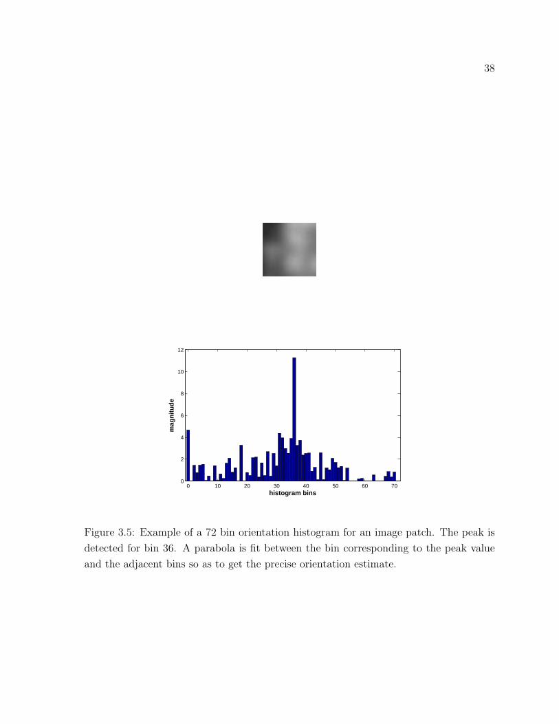
38
0 10 20 30 40 50 60 700
2
4
6
8
10
12
histogram bins
mag
nit
ud
e
Figure 3.5: Example of a 72 bin orientation histogram for an image patch. The peak is
detected for bin 36. A parabola is fit between the bin corresponding to the peak value
and the adjacent bins so as to get the precise orientation estimate.
39
The two approaches also differ in the way the scale-space representation is built to
detect the Hessian-Laplace points. This difference lies in the number of scales chosen
to built the scale-space representation and the scale factor between adjacent scale-space
images. For the SIHL detector, 11 images are used in the scale space representation (17
were used for the HL detector) and a factor of 1.3 was chosen between adjacent images
(1.2 was used for the HL detector).
Another difference between the two approaches arises due to different methods used
for estimating the orientation of feature points. The HL detector uses a method[54, 2002]
which is based on calculating the average of the Gaussian weighted gradient orientations
in a patch around the point. The approach used to assign orientation for points detected
with the SIHL detector is a modification of the approach proposed by Lowe[47, 2004].
Although these methods used to compute orientation do not influence the location and
scale of the points detected, they do however have an affect on the description of the
points (discussed in Chapter 4). This in turn affects the correspondences obtained using
those points.
3.3 Repeatability Criterion
Repeatability is one of the most important criteria used for evaluating the stability of
feature detectors. It measures the ability of a detector to extract the same feature points
across images irrespective of imaging conditions (this is the stability criterion as discussed
in section 2.1). Repeatability is measured by calculating the number of repeatable points
between images, according to the following definition. Given a point P in 3D space and
its projection p1 and p2 in two images, the points are termed repeatable if both p1 and
p2 are detected. The number of such repeatable feature points can be estimated between
two images if the mapping between the images is known. The repeatability of feature
points directly affects the number of correspondences that can be found between images.
Repeatability rate can be defined as the ratio of repeatable points between two images
to the total number of points detected. The total number of detected points corresponds
to the minimum number of points extracted from either image. Since the images used
for computing repeatability are taken under different imaging conditions, the part of the
3D scene represented by these images can be different. This implies that some points
detected in one image will have no corresponding points in the other image thus lead-
ing to an incorrect estimate of repeatability. Hence, while computing the repeatability
measure, only points that lie in the common region between two images are considered.

40
This common region is computed by using a homography[27, 2004], which is a 2D trans-
formation that defines the relationship between two images. Since the image datasets
evaluated here (discussed later) have been taken either by rotating the camera about its
optical center or by varying camera parameters like focal length and aperture, the image
points from all the images will lie on a plane in 3D space. This indicates that mapping
between two images can be described by using a homography (refer to Appendix C for
more information on homography).
Since there are image distortions, the corresponding point in the second image will not
be exactly where the homography predicts, but will lie in a region close to this prediction.
Hence a tolerance value is introduced for measuring repeatability to compensate for
localization errors. For two images I1 and I2 having feature points n1 and n2 in the
common region, the repeatability rate is defined as
Repeatability rate =n3
min(n1, n2)(3.6)
where n3 is the number of repeatable feature points computed between the two images
using n1 and n2.
In the context of scale invariant detectors, the scale parameter also has to be incor-
porated into the computation of repeatability. The scale of a point is used to associate
a region with a point proportional to its scale value. The regions are selected such that
they are centered at the point and their size is proportional to the scale of the point.
Hence, for scale invariant points repeatability can be described as a two stage procedure.
In the first stage, the homography between images is used to check for relative location
of points in the second image which is similar to what has been described before. Points
which lie in a certain tolerance range of their true value (true value refers to the predicted
location calculated using the homography) qualify for the next stage. In the second stage,
a score is computed which corresponds to the overlap between regions associated with
points that were previously selected. The overlap error for two points can be expressed
as
Overlap Error = |1− s2 min(σ21, σ
22)
max(σ21, σ
22)| (3.7)
where s is the actual scale factor between images retrieved from homography and σ1
and σ2 are the scale values of the points in the first and second image. Hence, in an ideal
condition where σ2=sσ1 we end up with an overlap error of zero, which indicates that
the two regions completely overlap. As the overlap error increases, the overlap between

41
the two regions decreases. A threshold on the overlap error is used to select the number
of repeatable points. Hence, repeatability is calculated by using the repeatability rate
for only those points which fit these two criteria.
3.3.1 Repeatability Tests
In this section we analyze the performance of different detectors using this repeatabil-
ity measure. Here we compare the performance of three detectors; the Difference of
Gaussian detector1 proposed by Lowe[47, 2004] and referred to as DOG, Hessian-Laplace
detector2 proposed by Mikolajczyk and Schmid[56, 2004]) and referred to as HL and the
Scale Interpolated Hessian-Laplace proposed in this research, referred to as SIHL. The
performance of the detectors is compared for two sequences3; for the first sequence the
images have undergone different amounts of scaling and rotation while for second data
set the illumination across the images is varied. For comparing these different detectors
we use the repeatability code provided by Mikolajczyk and Schmid on their webpage4.
The same code was also used by these authors for comparing the performance of various
affine region detectors[58, 2005].
A few notes on how the repeatability is computed and the parameters that can effect
repeatability. Every feature point in an image is associated with a circular region. The
region is selected such that it is centered on the point and its radius is proportional
to the scale of the point (Figure 3.2 shows the regions associated with feature points
detected at different scales). A pair of points is considered for computing repeatability
if the point in the second image lies within a tolerance range of its predicted value (the
value is predicted using homography as mentioned before). Here a tolerance level of
4σ is used where σ corresponds to the scale of the point in the first (reference) image.
Once the points have been selected, the overlap between different regions is used to
measure repeatability. Two points are deemed repeatable if the overlap error between
their respective regions is less than or equal to 40%.
There are two parameters that can affect the repeatability score between images; first
is the number of regions detected in both images and second is the size of those regions.
1DOG points are computed using the publicly available SIFT executable from David Lowe’s webpagehttp://www.cs.ubc.ca/ lowe/keypoints/
2The executable binaries have been taken from http://www.robots.ox.ac.uk/ vgg/research/affine/detectors.html3The image data sets were taken from http://www.robots.ox.ac.uk/ vgg/research/affine/. The
ground truth for all images with respect to the reference image is known.4http://www.robots.ox.ac.uk/ vgg/research/affine/evaluation.html
42
Detecting a smaller number of points leads to regions which are distinctive and stable.
A large number of regions on the other hand can at times clutter the scene and lead to
ambiguous matches where a single point in an image is matched to multiple points in
the other image. While evaluating the performance of affine detectors Mikolajczyk and
Schmid[58, 2005] observed that for some detectors the repeatability increased with an
increase in number of regions while for others it decreased. Since all the three detectors
that are being compared here detect the same type of points, increasing or decreasing the
number of points will change the repeatability for all detectors in the same fashion. This
indicates that ordering of the detectors based on repeatability results will stay the same
even if the number of points detected is changed. Here in order to improve the accuracy
of the results, we detect the same number of regions for all detectors in each image. This
facilitates the process of comparing matches obtained using different detectors.
The region size of the detected points can also have a significant impact on repeata-
bility as increasing the size of regions increases the repeatability. In order to overcome
this, for every region in the reference image, a scale factor is determined which maps the
region to a fixed region of radius 30 pixels. This scale factor is then multiplied to the
corresponding region in the other image before computing overlap score.
3.3.2 Scaling and Rotation Dataset
The scaling and rotation image set5 consists of 10 images (see Figure 3.6) where different
amounts of scaling (up to a scale factor of 4.4) and rotations are applied to the reference
image. This is a standard dataset that has been used by other authors to compare
scale and affine invariant feature detectors and descriptors[58, 2005][57, 2005]. Before
comparing repeatability results for different detectors for this dataset, we see the how
the localization performed for the SIHL detector affects the repeatability of points. We
compute repeatability for two images in this dataset (see Figure 3.6(a) and 3.6(e)) for
different overlap errors. Only points which have an overlap error value less than the
overlap error are deemed repeatable for that overlap error. Figure 3.7 shows the results
both in percentage terms and actual number of correspondences for SIHL detector with
and without localization. In general as the overlap error increases (the overlap criteria
is relaxed) more corresponding regions are found between images, thus giving higher
repeatability. The advantage of performing localization is evident from the graphs as
there is a significant difference between the two methods for an overlap error of 10%.
5The image dataset is available at http://lear.inrialpes.fr/people/mikolajczyk/
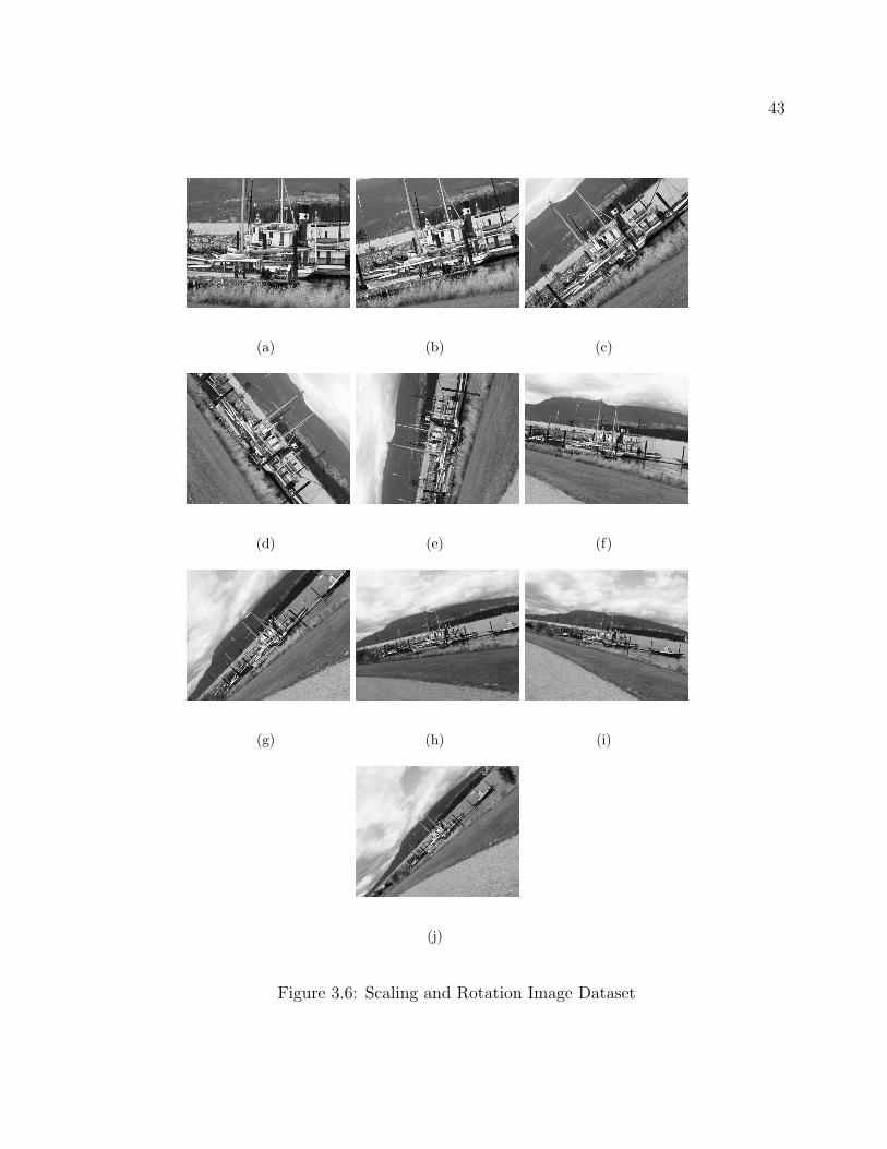
43
(a) (b) (c)
(d) (e) (f)
(g) (h) (i)
(j)
Figure 3.6: Scaling and Rotation Image Dataset

44
This indicates that performing scale localization does result in a more accurate scale
value for a keypoint which in turn leads to more accurate regions for points. For large
overlap errors, the change in size of an image region due to scale localization is less
noticeable due to relaxed overlap criteria thus resulting in equivalent repeatability scores
for both methods. Hence, this result indicates that localization is a crucial step in the
detection process of scale invariant features.
0 10 20 30 40 50 600
10
20
30
40
50
60
70
80
90
overlap error %
rep
eata
bili
ty %
SIHL detector with LocalizationSIHL detector without Localization
(a)
0 10 20 30 40 50 600
100
200
300
400
500
600
700
800
900
1000
overlap error %
no
. of
corr
esp
on
den
ces
SIHL detector with LocalizationSIHL detector without Localization
(b)
Figure 3.7: Repeatability results with and without localization for an image pair from
scaling and rotation image dataset (see Figure 3.6(a) and 3.6(e)) (a) Repeatability score
for different overlap errors (b) Number of correspondences using repeatability
We now give comparative results for the three detectors that have been mentioned
before. The repeatability is computed between the reference image and all the trans-
formed images for all the detectors. Figure 3.8 shows the repeatability in percentage and
the number of correspondences obtained for the different approaches. The results have
been shown for the scale factor parameter which corresponds to the scale ratio between
an image from the dataset and the reference image. The graphs shown here have been
obtained for an overlap error of 40%. In general, as the scale factor between the images
increases, fewer points are detected in the common region of the two images. Due to
this, the number of correspondences obtained steadily decreases. Also with increasing
scale factor, it is harder to detect points which correspond to the same image structure,
as at large scales some of the image structures become too small to be detected. Hence,
repeatability generally decreases with increasing scale.
Looking at the repeatability graph we observe that a better repeatability is obtained
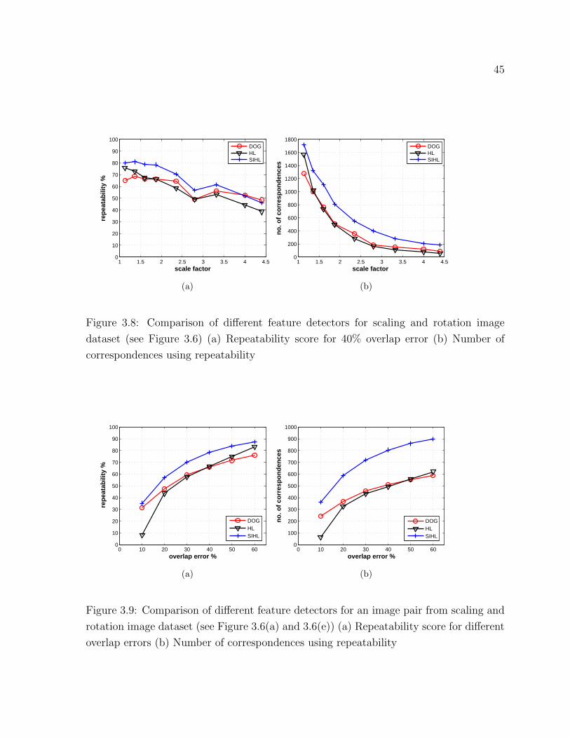
45
1 1.5 2 2.5 3 3.5 4 4.50
10
20
30
40
50
60
70
80
90
100
scale factor
rep
eata
bili
ty %
DOGHLSIHL
(a)
1 1.5 2 2.5 3 3.5 4 4.50
200
400
600
800
1000
1200
1400
1600
1800
scale factor n
o. o
f co
rres
po
nd
ence
s
DOGHLSIHL
(b)
Figure 3.8: Comparison of different feature detectors for scaling and rotation image
dataset (see Figure 3.6) (a) Repeatability score for 40% overlap error (b) Number of
correspondences using repeatability
0 10 20 30 40 50 600
10
20
30
40
50
60
70
80
90
100
overlap error %
rep
eata
bili
ty %
DOGHLSIHL
(a)
0 10 20 30 40 50 600
100
200
300
400
500
600
700
800
900
1000
overlap error %
no
. of
corr
esp
on
den
ces
DOGHLSIHL
(b)
Figure 3.9: Comparison of different feature detectors for an image pair from scaling and
rotation image dataset (see Figure 3.6(a) and 3.6(e)) (a) Repeatability score for different
overlap errors (b) Number of correspondences using repeatability
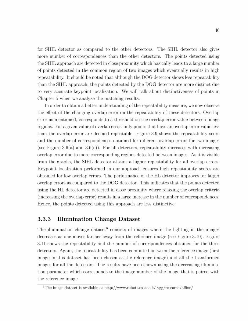
46
for SIHL detector as compared to the other detectors. The SIHL detector also gives
more number of correspondences than the other detectors. The points detected using
the SIHL approach are detected in close proximity which basically leads to a large number
of points detected in the common region of two images which eventually results in high
repeatability. It should be noted that although the DOG detector shows less repeatability
than the SIHL approach, the points detected by the DOG detector are more distinct due
to very accurate keypoint localization. We will talk about distinctiveness of points in
Chapter 5 when we analyze the matching results.
In order to obtain a better understanding of the repeatability measure, we now observe
the effect of the changing overlap error on the repeatability of these detectors. Overlap
error as mentioned, corresponds to a threshold on the overlap error value between image
regions. For a given value of overlap error, only points that have an overlap error value less
than the overlap error are deemed repeatable. Figure 3.9 shows the repeatability score
and the number of correspondences obtained for different overlap errors for two images
(see Figure 3.6(a) and 3.6(e)). For all detectors, repeatability increases with increasing
overlap error due to more corresponding regions detected between images. As it is visible
from the graphs, the SIHL detector attains a higher repeatability for all overlap errors.
Keypoint localization performed in our approach ensures high repeatability scores are
obtained for low overlap errors. The performance of the HL detector improves for larger
overlap errors as compared to the DOG detector. This indicates that the points detected
using the HL detector are detected in close proximity where relaxing the overlap criteria
(increasing the overlap error) results in a large increase in the number of correspondences.
Hence, the points detected using this approach are less distinctive.
3.3.3 Illumination Change Dataset
The illumination change dataset6 consists of images where the lighting in the images
decreases as one moves farther away from the reference image (see Figure 3.10). Figure
3.11 shows the repeatability and the number of correspondences obtained for the three
detectors. Again, the repeatability has been computed between the reference image (first
image in this dataset has been chosen as the reference image) and all the transformed
images for all the detectors. The results have been shown using the decreasing illumina-
tion parameter which corresponds to the image number of the image that is paired with
the reference image.
6The image dataset is available at http://www.robots.ox.ac.uk/ vgg/research/affine/

47
(a) (b)
(c) (d)
(e) (f)
Figure 3.10: Illumination Change Image Dataset
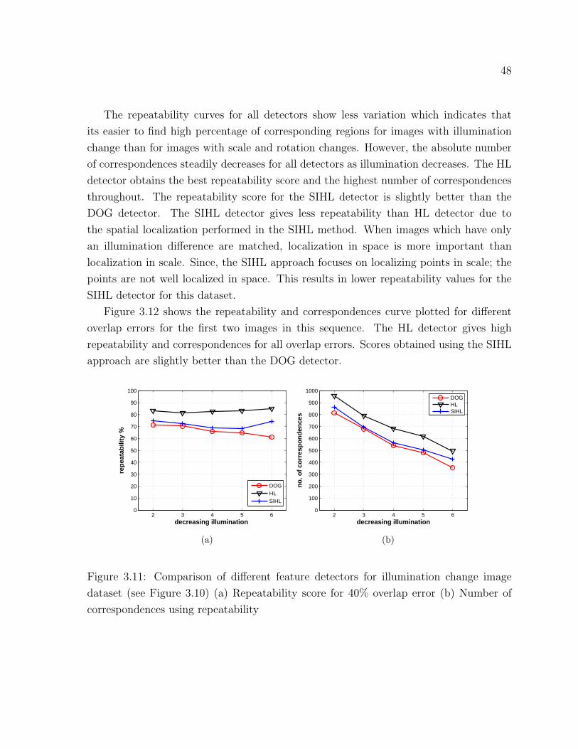
48
The repeatability curves for all detectors show less variation which indicates that
its easier to find high percentage of corresponding regions for images with illumination
change than for images with scale and rotation changes. However, the absolute number
of correspondences steadily decreases for all detectors as illumination decreases. The HL
detector obtains the best repeatability score and the highest number of correspondences
throughout. The repeatability score for the SIHL detector is slightly better than the
DOG detector. The SIHL detector gives less repeatability than HL detector due to
the spatial localization performed in the SIHL method. When images which have only
an illumination difference are matched, localization in space is more important than
localization in scale. Since, the SIHL approach focuses on localizing points in scale; the
points are not well localized in space. This results in lower repeatability values for the
SIHL detector for this dataset.
Figure 3.12 shows the repeatability and correspondences curve plotted for different
overlap errors for the first two images in this sequence. The HL detector gives high
repeatability and correspondences for all overlap errors. Scores obtained using the SIHL
approach are slightly better than the DOG detector.
2 3 4 5 60
10
20
30
40
50
60
70
80
90
100
decreasing illumination
rep
eata
bili
ty %
DOGHLSIHL
(a)
2 3 4 5 60
100
200
300
400
500
600
700
800
900
1000
decreasing illumination
no
. of
corr
esp
on
den
ces
DOGHLSIHL
(b)
Figure 3.11: Comparison of different feature detectors for illumination change image
dataset (see Figure 3.10) (a) Repeatability score for 40% overlap error (b) Number of
correspondences using repeatability
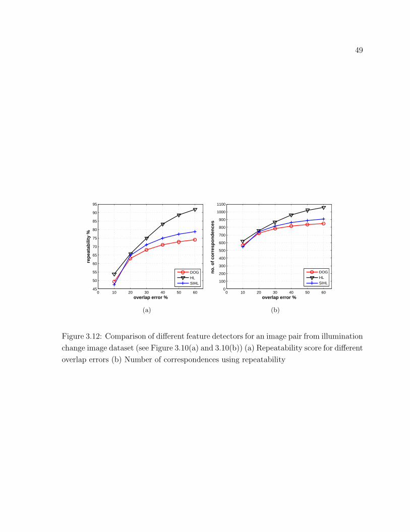
49
0 10 20 30 40 50 6045
50
55
60
65
70
75
80
85
90
95
overlap error %
rep
eata
bili
ty %
DOGHLSIHL
(a)
0 10 20 30 40 50 600
100
200
300
400
500
600
700
800
900
1000
1100
overlap error %
no
. of
corr
esp
on
den
ces
DOGHLSIHL
(b)
Figure 3.12: Comparison of different feature detectors for an image pair from illumination
change image dataset (see Figure 3.10(a) and 3.10(b)) (a) Repeatability score for different
overlap errors (b) Number of correspondences using repeatability
Chapter 4
Feature Descriptors for Matching
Having extracted features from an image, the next step in any matching or recognition
application requires associating every feature with a unique identifier or a signature
which can be used to identify the feature from a database. These identifiers or signatures
used to describe features are termed as feature descriptors. Such descriptors have been
widely used in a large number of applications like object recognition[47, 2004], texture
classification[2003][39], image indexing[65, 1997], generation of panoramas[9, 2003], wide
baseline matching[4, 2000] and many more.
Creating a descriptor requires capturing the characteristics of the local region of pixels
around a point. Depending upon the application these characteristics could be grayscale
or color values of the region, texture or shape of the local region. The task of a descriptor
is to represent these characteristics as compactly as possible, yet at the same time be
distinctive enough to associate a feature with its correct match.
A key attribute of descriptors that is vital in determining their robustness, relates
to their ability to handle different geometric and photometric transformations. Ideally,
descriptors are designed such that they are invariant to changes in image scale and image
rotation. Invariance to changes in image viewpoint is also incorporated where affine
invariance is desired. On the photometric side the descriptors should be insensitive to
changes in illumination including non-linear illumination. In addition to these properties,
the descriptor should also be robust to errors in localization of features and should not
be affected by partial occlusions. Thus, invariance to all these classes of transformations
ensures that changes in lighting conditions and camera parameters will not produce a
large change in feature descriptor.
In the literature, numerous descriptors have been proposed to describe the local image
50
51
pattern around a point. In this chapter, we will primarily focus on descriptors that have
been introduced to characterize scale and affine invariant features. The next section
gives a brief overview of some of the techniques that have been developed for computing
descriptors followed by a detailed description of descriptors that are most relevant in
the context of this research, namely SIFT[47, 2004] and PCA-SIFT[34, 2004]. In this
chapter we also introduce a novel method to apply Haar descriptors which are computed
using the Haar wavelet transform. These descriptors offer the advantage that they are
computationally less expensive to compute and smaller in size when compared to other
descriptors. This in turn makes them an interesting choice for image matching and image
retrieval applications. In the next chapter, we propose different configurations of Haar
descriptors and evaluate them along with other descriptors.
4.1 Related Work
This section introduces some of the algorithms that have been proposed to compute de-
scriptors for scale and affine invariant features. Of all the methods proposed in literature,
one of the simplest ways to compute a descriptor is by representing the local gray scale
pattern around a point in the form of a feature vector. This feature vector can then be
matched to another feature vector by using the cross correlation measure[28, 1996]. Al-
though such descriptors can be used to generate reasonably good representations of the
local neighborhood around points, the large size of the descriptors makes it impractical
to be used for recognition applications, especially retrieval applications where smaller
descriptors are necessary.
A method frequently used for generating descriptors involves representing the char-
acteristics of the local patch as a histogram. We discuss some of these methods that have
used different histograms to compute descriptors.
Belongie et al.[6, 2002] proposed a descriptor known as shape context to find corre-
sponding regions using shape information. Their method is based on extracting edges
and constructing shape contexts for a chosen set of reference points along those edges.
In order to compute the feature descriptor, a log polar histogram of edge point locations
and orientations is generated where the locations are described relative to the reference
point. The bins for the histogram are spaced in such a way so that the histogram is more
sensitive to samples closer to the reference point than those that are far away. A similar
descriptor based on log polar histogram was also used by Qin and Gao[63, 2005] to find
correspondences between images.

52
Spin Images were introduced by Johnson and Herbet[30, 1999] to perform object
recognition for cluttered 3D scenes. Their objective was to match surfaces by matching
individual surface points where each surface point was represented by a spin image.
In order to generate spin images, the local neighborhood around each surface point
was represented as a 2D histogram. The histogram was computed using two distance
parameters which were measured from other surface points. The spin images were thus
a mapping of relative positions of 3D surface points on to a 2D plane and represent
the shape of the object. This concept was further extended for texture classification by
Lazebnik et al.[39, 2003] where a novel descriptor called an intensity domain spin image
was introduced. The idea there was to encode a normalized image patch as a histogram
of pixel distances and intensity values where the pixel distances were measured from the
center of the patch. The descriptor was shown to perform texture recognition for a wide
range of geometric transformations including viewpoint changes.
Ling and Jacobs[45, 2005] introduced a novel descriptor which was invariant to general
deformations in images. The problem of deformation was addressed using Geodesic
Intensity Histogram where the basic idea was to have both the histogram parameters,
namely geodesic distance1 and intensity, invariant to image deformation. In order to
compute the geodesic distances between points in an image, the image was represented
as a surface where the third dimension referred to the intensity value of the image. Then
for each keypoint in the image, a histogram was computed using a set of points in its
vicinity where the points had been selected by a sampling method. The method was
shown to perform better than all other methods for finding correspondences in deformed
images.
Some other descriptors that have been based on histograms include the SIFT descriptor[47,
2004]. This uses the gradient information around a point to generate orientation his-
tograms which are in turn used to create the descriptor. Pairwise Geometric Histograms[3,
1995] are created for line segments by measuring the perpendicular distances and relative
angles from other line segments in the image.
Another class of algorithms that have been used to compute descriptors use im-
age derivatives of certain orders to represent a point’s neighborhood. Freedman and
Adelson[25, 1991] proposed the concept of Steerable Filters which can be used to steer
the response of a filter in any orientation. This was used to compute the local image
derivatives for a point for various orientations, thus resulting in a descriptor which was
invariant to image rotation. The derivatives were computed by performing convolution
1Geodesic distance is the distance of the shortest path between two points on a surface

53
with Gaussian derivatives. Some other prominent descriptors proposed along similar
lines include differential invariants[37, 1987] where the descriptor is computed by con-
volving the image with set of Gaussian derivatives. Similarly, complex filters[64, 2002]
use a set of filters similar to derivatives of Gaussian to obtain a descriptor invariant to
geometrical transformations and affine intensity variations.
Apart from these descriptors other approaches based on Gabor filters and wavelets
have also been explored in the literature. Some of the wavelet based descriptors will be
discussed later in this chapter.
All the three descriptors analyzed in this research have been designed for scale in-
variant points. Each scale invariant feature point is associated with four parameters
namely x,y location of the point, a scale value and an orientation value. The scale and
orientation of the point are used to make the descriptor invariant to image scaling and
rotation. This is done by selecting a square image patch around a point whose size is
proportional to the scale of the point, and which has been rotated depending upon the
point’s orientation. Once the effect of scaling and rotation has been negated, the values
inside the patch are used to make the descriptor. We now discuss in detail the three
descriptors analyzed here.
4.2 SIFT Descriptor
The SIFT (Scale Invariant Feature Transform) descriptor proposed by Lowe[47, 2004][46,
1999] has been one of the most widely used descriptors. In a survey done to compare
the performance of different descriptors by Mikolajczyk and Schmid[57, 2005], SIFT was
shown to perform better than all other local descriptors.
The SIFT descriptor is based on the idea of using the local gradient patch around a
point to build a representation for the point. This representation is built by generating
multiple orientation histograms for the patch. Given a feature point in the image and
a square patch around it which has been appropriately scaled and rotated, the gradient
magnitudes and orientations in the patch are used to generate orientation histograms
over a 4x4 region. For each orientation histogram 8 bins are used. The final descriptor
is computed by concatenating the outputs of 16 orientation histograms which results
in a 128 element feature descriptor. Figure 4.1 shows a set of orientation histograms
generated for one such gradient patch.
In order to improve the robustness of the SIFT descriptor, a number of measures
are incorporated into the construction of the orientation histograms. One such measure

54
Figure 4.1: Orientation Histograms for a gradient patch over a 4x4 region
involves weighting the magnitude of gradient samples by a Gaussian function centered
around the keypoint before the samples are added to the orientation histograms. This
ensures that samples which are closer to the center and are more important are assigned
more weight. It also makes the descriptor less sensitive to small positional shifts in the
local patch. Another measure which also helps to make the descriptor more resilient to
localization errors is to distribute the gradient samples to adjacent histogram bins using
trilinear interpolation. This helps to overcome the boundary effect problem where a shift
in gradient sample from one histogram to another or from one orientation to another in
the same histogram produces a sudden change in a descriptor.
Figure 4.2 shows how a gradient sample is distributed between adjacent histograms
and orientations. The red arrow in the left image indicates the gradient sample where
its direction corresponds to the sample’s orientation. The bins to which this sample
contributes are marked as red in the right image.
The last stage of SIFT requires making the descriptor invariant to changes in image
illumination. Normalizing the descriptor to unit length helps in overcoming any bright-
ness or contrast changes that may have occurred in the image. However, this doesn’t
get rid of the non-linear illumination changes that may have taken place. To overcome
such changes, a thresholding operation is performed to restrict the maximum gradient
magnitude of the descriptor followed by a normalization operation. A value of 0.2 was
proposed by the author as the most optimum threshold.
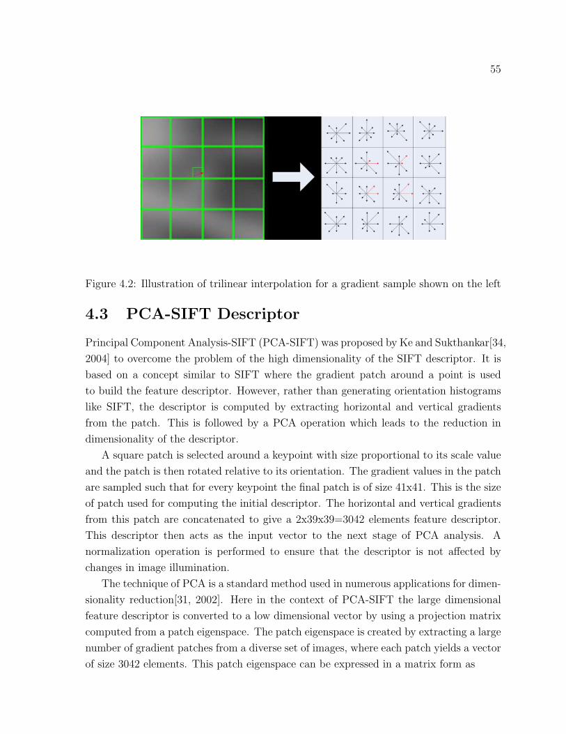
55
Figure 4.2: Illustration of trilinear interpolation for a gradient sample shown on the left
4.3 PCA-SIFT Descriptor
Principal Component Analysis-SIFT (PCA-SIFT) was proposed by Ke and Sukthankar[34,
2004] to overcome the problem of the high dimensionality of the SIFT descriptor. It is
based on a concept similar to SIFT where the gradient patch around a point is used
to build the feature descriptor. However, rather than generating orientation histograms
like SIFT, the descriptor is computed by extracting horizontal and vertical gradients
from the patch. This is followed by a PCA operation which leads to the reduction in
dimensionality of the descriptor.
A square patch is selected around a keypoint with size proportional to its scale value
and the patch is then rotated relative to its orientation. The gradient values in the patch
are sampled such that for every keypoint the final patch is of size 41x41. This is the size
of patch used for computing the initial descriptor. The horizontal and vertical gradients
from this patch are concatenated to give a 2x39x39=3042 elements feature descriptor.
This descriptor then acts as the input vector to the next stage of PCA analysis. A
normalization operation is performed to ensure that the descriptor is not affected by
changes in image illumination.
The technique of PCA is a standard method used in numerous applications for dimen-
sionality reduction[31, 2002]. Here in the context of PCA-SIFT the large dimensional
feature descriptor is converted to a low dimensional vector by using a projection matrix
computed from a patch eigenspace. The patch eigenspace is created by extracting a large
number of gradient patches from a diverse set of images, where each patch yields a vector
of size 3042 elements. This patch eigenspace can be expressed in a matrix form as
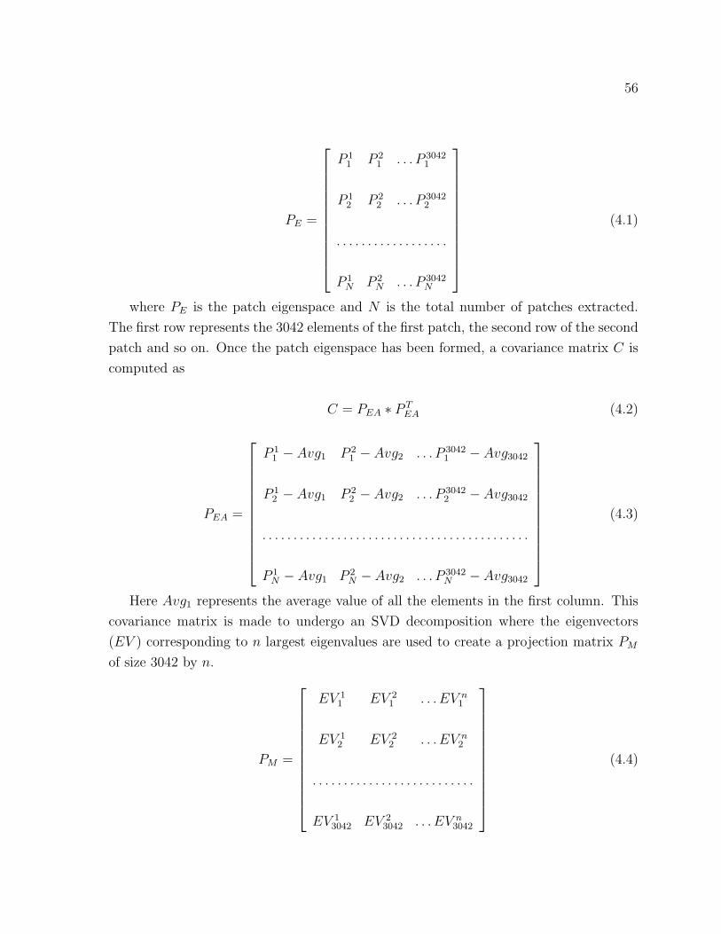
56
PE =
P 11 P 2
1 . . . P 30421
P 12 P 2
2 . . . P 30422
. . . . . . . . . . . . . . . . . .
P 1N P 2
N . . . P 3042N
(4.1)
where PE is the patch eigenspace and N is the total number of patches extracted.
The first row represents the 3042 elements of the first patch, the second row of the second
patch and so on. Once the patch eigenspace has been formed, a covariance matrix C is
computed as
C = PEA ∗ P TEA (4.2)
PEA =
P 11 − Avg1 P 2
1 − Avg2 . . . P 30421 − Avg3042
P 12 − Avg1 P 2
2 − Avg2 . . . P 30422 − Avg3042
. . . . . . . . . . . . . . . . . . . . . . . . . . . . . . . . . . . . . . . . . . .
P 1N − Avg1 P 2
N − Avg2 . . . P 3042N − Avg3042
(4.3)
Here Avg1 represents the average value of all the elements in the first column. This
covariance matrix is made to undergo an SVD decomposition where the eigenvectors
(EV ) corresponding to n largest eigenvalues are used to create a projection matrix PM
of size 3042 by n.
PM =
EV 11 EV 2
1 . . . EV n1
EV 12 EV 2
2 . . . EV n2
. . . . . . . . . . . . . . . . . . . . . . . . . .
EV 13042 EV 2
3042 . . . EV n3042
(4.4)

57
This projection matrix along with the average values computed previously are used
to perform the PCA operation. In this research, the projection matrix is similar to the
one used by the original authors where the value of n is 36. Hence, the final descriptors
generated by PCA-SIFT are of length 36.
4.4 Wavelet Descriptors
Wavelet transform has been frequently used for multi-resolution analysis of images in
order to perform compression, feature extraction and texture analysis. One of the fac-
tors that has contributed to the widespread use of wavelets is its good time(space)-
frequency(scale) localization. While reduction in bandwidth of the image requires good
localization in scale so as to maintain the fidelity of data, preserving patterns present in
the image requires good localization in space. It is the ability of wavelets to generate a
compact representation of an image, that is of particular interest when they are used to
represent local image structures.
Amongst all the different wavelet basis, Haar wavelets2 are the ones that are most
commonly used for computing descriptors. This frequent use of Haar wavelets arises
from that fact that Haar basis functions are computationally very easy to implement.
The basis functions for Haar can be numerically expressed as
ψji (x) = ψ(2jx− i) i = 0, ...., 2j − 1 (4.5)
or in the normalized form as
ψji (x) = 2j/2ψ(2jx− i) i = 0, ...., 2j − 1 (4.6)
where
ψ(x) =
1 for 0 ≤ x < 1/2
−1 for 1/2 ≤ x < 1
0 otherwise
(4.7)
Figure 4.3 shows the Haar basis ψ10 and ψ1
1. The above notation represents the Haar
basis functions in one dimension. Then given a one dimensional signal, its representation
in terms of Haar basis can be written as
2It should be noted that Haar wavelets do not have good time-frequency localization due to theirdiscontinuous nature.

58
f(x) =∞∑
i=−∞cj′i φj′
i (x) +∞∑
i=−∞
∞∑j=j′
djiψ
ji (x) (4.8)
where
φji (x) = φ(2jx− i) i = 0, ...., 2j − 1 (4.9)
φ(x) =
{1 for 0 ≤ x < 1
0 otherwise(4.10)
0 0.5 1
−1
0
1
(a)
0 0.5 1
−1
0
1
(b)
Figure 4.3: Haar basis functions (a) ψ10 (b) ψ1
1
Here j′ is the starting scale. The functions φji (x) are known as the scaling functions.
The coefficients cji associated with the scaling functions are used to represent the average
values. The coefficients dji of the wavelet functions represent the detail coefficients which
can be used along with the average values to reconstruct the original signal. Thus by
using Haar wavelets, we are trying to represent a signal at set of coarser resolutions
where every coarse scale representation is associated with a set of coefficients which can
be used to obtain the previous finer scale version of the signal. The decomposition of the
signal to coarser resolutions is obtained by taking an average between successive samples
of the signal. The detail coefficients, on the other hand, are obtained by computing the
difference between successive signal samples. Both these operations constitute the Haar
wavelet transform.

59
A similar decomposition can also be applied to two dimensional signals. Given an
image patch of some size along with the Haar basis functions, the computation of Haar
coefficients can be performed in two ways. For the standard decomposition method, the
one dimensional wavelet transform is applied to each row in the image till we are left with
just one average coefficient. Then, in the next step, the wavelet transform operation is
performed along every column in the image. This leaves us with one average coefficient for
the whole image along with detail coefficients for every resolution. In the non-standard
method of decomposition, the transform on rows and columns is performed alternately.
First a single step of averaging and difference is performed for successive pixels for each
row in the image. Then, the same type of decomposition is carried for each column in
the image. This process is performed iteratively, till we are left with a single average
coefficient. Although the standard decomposition method is easier to implement, in
practice the non-standard method is faster and more efficient. Figure 4.4 shows the non-
standard decomposition applied on an image patch. A more detailed discussion of Haar
wavelet basis can be found in the work by Stollinitz et al.[67, 1995]
In the context of image features, the objective of using Haar basis is to represent the
image patch around a feature in terms of Haar coefficients. The idea is that some of
the detail coefficients can be neglected without losing too much information about the
patch. An important feature of the Haar basis functions in the same context is their
orthogonality property. This property helps to preserve Euclidean distances between
feature descriptors when a feature descriptor is transformed using Haar basis functions.
Thus, the Euclidean distance measure can be applied directly on Haar descriptors to find
the nearest neighbor.
We now mention some of the methods that have used Haar wavelets to compute
descriptors. Krishnamachari and Mottaleb[38, 2000] proposed a method to perform im-
age retrieval and match video segments using a descriptor computed from Haar basis
functions. Their method is based on extracting color histogram of an image and convert-
ing it into a 63 bit descriptor of Haar transform coefficients. A quantization operation
is performed so as to convert the descriptor coefficients into binary form. This binary
descriptor is then used as an index to perform image retrieval from a database. Utenpat-
tanant et al.[74, 2006] proposed a method using the same descriptor along with a pruning
technique for their retrieval application. The addition of pruning method showed faster
retrieval than the previous method.
Brown et al.[10, 2005] developed a method for matching images where a 8x8 patch
of sampled intensity values extracted for a point, was converted to a 64 bit descriptor of

60
Figure 4.4: Non-standard decomposition method of wavelet transform. All the sub
images inside an image (except the average image) have been amplified by a factor of 2
for display purposes.
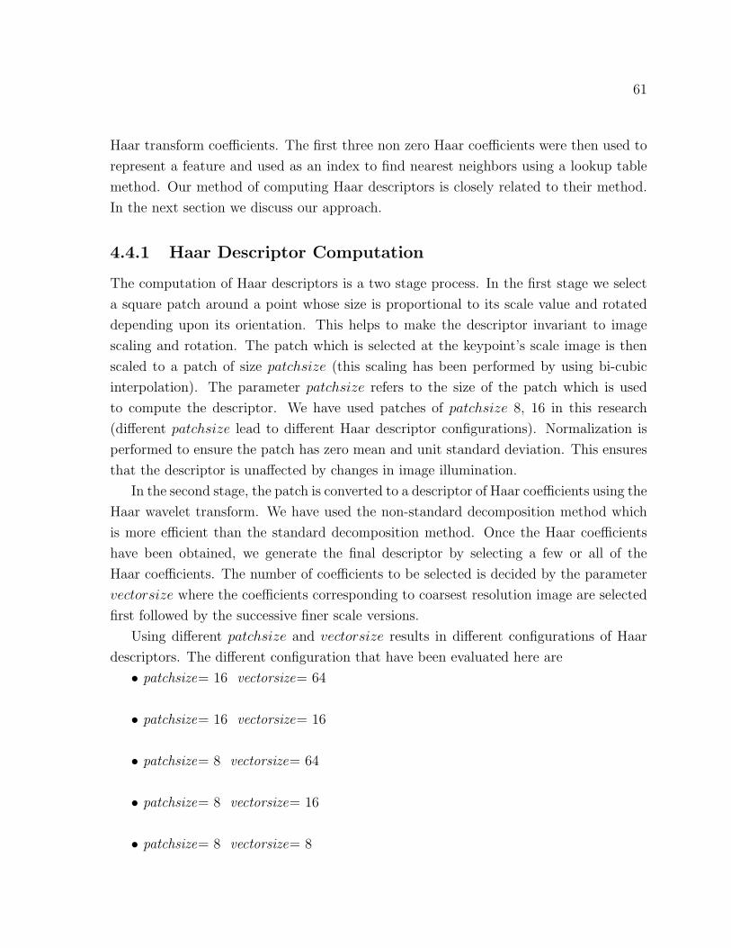
61
Haar transform coefficients. The first three non zero Haar coefficients were then used to
represent a feature and used as an index to find nearest neighbors using a lookup table
method. Our method of computing Haar descriptors is closely related to their method.
In the next section we discuss our approach.
4.4.1 Haar Descriptor Computation
The computation of Haar descriptors is a two stage process. In the first stage we select
a square patch around a point whose size is proportional to its scale value and rotated
depending upon its orientation. This helps to make the descriptor invariant to image
scaling and rotation. The patch which is selected at the keypoint’s scale image is then
scaled to a patch of size patchsize (this scaling has been performed by using bi-cubic
interpolation). The parameter patchsize refers to the size of the patch which is used
to compute the descriptor. We have used patches of patchsize 8, 16 in this research
(different patchsize lead to different Haar descriptor configurations). Normalization is
performed to ensure the patch has zero mean and unit standard deviation. This ensures
that the descriptor is unaffected by changes in image illumination.
In the second stage, the patch is converted to a descriptor of Haar coefficients using the
Haar wavelet transform. We have used the non-standard decomposition method which
is more efficient than the standard decomposition method. Once the Haar coefficients
have been obtained, we generate the final descriptor by selecting a few or all of the
Haar coefficients. The number of coefficients to be selected is decided by the parameter
vectorsize where the coefficients corresponding to coarsest resolution image are selected
first followed by the successive finer scale versions.
Using different patchsize and vectorsize results in different configurations of Haar
descriptors. The different configuration that have been evaluated here are
• patchsize= 16 vectorsize= 64
• patchsize= 16 vectorsize= 16
• patchsize= 8 vectorsize= 64
• patchsize= 8 vectorsize= 16
• patchsize= 8 vectorsize= 8

62
For the first configuration, a patchsize of 16 results in a descriptor of 256 Haar coef-
ficients where only the first 64 coefficients have been used to create the final descriptor.
The purpose of using Haar descriptors is to investigate the possibility of using small size
descriptors for representing image features. Although these descriptors are less robust to
errors in localization of points when compared with the SIFT descriptor, the goal here
is to see if these descriptors are still robust enough to give good matches. In the next
chapter, we will give the results for the different configurations of Haar descriptors that
we have analyzed in this research.
4.5 Similarity Measures
A similarity measure is a measure of distance which is used to compute the proximity
of descriptors in a high dimensional feature space. This proximity measure can be used
to recognize descriptors which are similar and therefore correspond to the same image
structure.
Amongst the numerous similarity measures proposed in the literature, one of the most
widely used measures is the Mahalanobis distance. The Mahalanobis distance is used to
compute distance between descriptors when the descriptor elements have different ranges
and different amounts of variation. It is commonly used when the correlation between
different descriptor elements has to be taken into account. Given two descriptors d1 and
d2, the Mahalanobis distance between them is
DM =√
(d1 − d2)T Σ−1(d1 − d2) (4.11)
where Σ is the covariance matrix
The Euclidean distance is one of the simplest similarity measures used to find prox-
imity in a high dimensional feature space. It can be defined as the square root of the
sum of squared differences between the corresponding components of two descriptors.
DE =√
(d1 − d2)T (d1 − d2) (4.12)
The Euclidean distance can be expressed in vector form as
DE =√∑
(d1[i]− d2[i])2 (4.13)

63
As it can be seen from the first two equations, the Mahalanobis distance is equivalent
to the Euclidean distance if the covariance matrix is an identity matrix.
The similarity measures discussed previously find the best match for a descriptor
by locating its nearest neighbor in a database. However, this can at times result in
erroneous correspondences for descriptors which are associated with features arising from
background clutter. A similarity measure used in SIFT based on ratio of Euclidean
distances, has been shown to overcome this problem. The measure is calculated by
computing the ratio of distance to the closest and the second closest neighbor for a given
descriptor. It is assumed that the nearest neighbor is a correct match while the second
nearest is an incorrect match. It has been shown that it is easier to differentiate between
correct and incorrect matches using this measure based on ratio of distances rather than
using the distance of nearest neighbor alone.
The SIFT descriptor has shown to perform better when the similarity measure used is
distance ratio matching, while the PCA-SIFT descriptor gives better results for nearest
neighbor matching[57, 2005]. We will confirm these results experimentally in the next
chapter, when we compare the performance of different descriptors for both nearest
neighbor similarity measure and distance ratio measure.

Chapter 5
Image Matching and Retrieval
Image matching is one of the fundamental tasks in computer vision. A good set of
correspondences between images is essential in order to carry out certain tasks. Matching
also constitutes an important step in content based image retrieval applications where
we are interested in retrieving images similar to a query image.
In this chapter, we give experimental results for two sets of experiments; image match-
ing and image retrieval. For image matching experiments, we compare the performance
of different matching algorithms on two image datasets (the ground truth for the datasets
is known). These algorithms have been constructed using a combination of different de-
tectors and descriptors that have been described in previous chapters. We analyze the
matches obtained for different techniques and evaluate their performance for different
evaluation metrics. The objective here is to identify the best matching strategy amongst
all the different configurations.
The latter part of this chapter discusses the problem of image retrieval, which is an
application of image matching to the field of content based image retrieval. Unlike the
image matching experiments, the images used to perform image retrieval are panoramic
images. The panoramic images used have been captured at different spatial locations
and along different paths. Given a query image, we use the matching strategy developed
in this research to retrieve an image from the database which is most similar to the
query. This is done by selecting the image which gives the maximum number of matches
with the query image. The objective of performing such a retrieval application is to
find images which correspond to the intersection points or are closest to the intersection
points between different panoramic sequences (explained in detail later in this chapter).
In contrast with the image matching experiments, since the transformations between
64
65
different panoramic images are not known, the matches obtained are refined using the
Random Sample Consensus (RANSAC) method before deciding on the closest image.
5.1 Evaluation Metrics
Various evaluation metrics have been proposed in the literature for analyzing matches.
The type of matches obtained can be used to assess the performance of a feature matching
strategy. Most of these metrics compute a score based on the percentage of correct and
false matches obtained. Here, we evaluate our results using two evaluation metrics.
For the first metric, we compute the number of correct matches obtained for various
matching algorithms in both absolute and relative terms. This metric for evaluation was
proposed by Mikolajczyk and Schmid1[58, 2005] to compare the performance of various
affine region detectors when combined with the SIFT descriptor.
Every point in an image is associated with a circular region and a descriptor (the
descriptor has been computed using the circular region). The region is selected such
that it is centered on the point and its radius is proportional to the scale of the point.
Two points are said to be matched if the overlap error between their respective regions
is below 50% and the Euclidean distance between their descriptors is below a threshold.
Overlap error corresponds to a threshold set on the value of overlap score computed
between two regions (mentioned in Section 3.5). The ground truth for a pair of images
is used to compute the overlap error. The matching here is based on finding the nearest
neighbor in descriptor space.
Since we are directly using the ground truth to decide a match, the matches obtained
are all correct matches. Once we have the number of correct matches, we compute the
matching score, which is defined as the ratio of correct matches to the number of detected
regions.
matching score =number of correct matches
number of detected regions(5.1)
Here the number of regions detected is the smallest number of regions for a pair of
images. Since, the number of points detected using all detectors is the same for an image,
the denominator of the above expression stays the same for an image pair being evaluated
using different matching configurations (see next section for matching configurations).
1We use the original source code from the author’s websitehttp://www.robots.ox.ac.uk/ vgg/research/affine/evaluation.html
66
In any matching application, not only are we interested in knowing the number of
correct matches but also the number of false matches obtained. The simultaneous anal-
ysis of correct and false matches can be used to evaluate the accuracy of a matching
algorithm. The metric which is widely used for performing such analysis is based on
measuring recall and 1-precision[11, 1994][2, 2002]. The correct and false matches are
analyzed by this metric for different values of the matching threshold. For any given
dataset, recall can be defined as the number of correct positives detected relative to the
total number of positives present in the dataset.
recall =number of correct positives
total number of positives in the data set(5.2)
The recall parameter gives the positive detection rate for the dataset. The precision
on the other hand is defined as the number of correct positives detected to the total
number of positives detected (total number of positives will include both correct and
false positives)
precison =number of correct positives
number of correct positives + number of false positives(5.3)
The precision parameter describes the number of correct detections relative to the
total number of detections. Since in a matching task we are more interested in knowing
the number of false detections relative to the total number of detections, we make use of
the 1-precision parameter
1− precison =number of false positives
number of correct positives + number of false positives(5.4)
In the context of our research, a correct positive corresponds to a correct match
between the two images while a false positive refers to a false match. The total number
of positives in the datset refers to the total number of correct matches that can be found,
which is the number of correspondences obtained using repeatability. Using the above
definitions we redefine recall and 1- precision as
recall =number of correct matches
number of correspondences(5.5)
1− precision =number of false matches
total number of matches(5.6)

67
The ideal recall vs 1-precision curve is a vertical line which starts at zero recall and
goes up to a recall value of one for a zero value of 1-precision and is horizontal thereafter.
However, in any scenario due to image distortions and non repeatable points we will get
false matches before we reach a recall of one. The next best thing is to have a curve
which has a high value of recall for any value of 1- precision. Usually, as the threshold
parameter is relaxed, the number of correct matches increases which in turn increases
the recall. If the recall value doesn’t improve with a change in threshold, this indicates
that the remaining points correspond to different structures in the image and cannot
be matched. Another factor which can lead to non increasing recall is distinctiveness
of descriptors. In cases where images to be matched are composed of similar looking
structures, non distinctive descriptors are unable to distinguish them thus resulting in
false matches. Hence, the recall vs 1- precision curves indicate the tradeoff that exists
between correct and false matches for the threshold parameter. If we adjust the threshold
to have more matches, then we also increase the number of false matches and vice-versa.
5.2 Different Matching Configurations
Any matching algorithm consists of two distinct entities, namely the feature detector and
the feature descriptor. The feature detector is used to detect points in an image while
the feature descriptor is used to generate a description for these points. This description
is used to identify similar points between images. Here we use the above mentioned
metrics to evaluate the performance of different detectors when combined with different
descriptors. The different configurations evaluated in this research are given below
• Difference of Gaussian (DOG) detector + SIFT/PCA-SIFT descriptor2 3
• Hessian-Laplace (HL) detector + SIFT/PCA-SIFT descriptor4
• Scale Interpolated Hessian-Laplace (SIHL) detector (our Hessian-Laplace approach)
2For computing SIFT descriptors for DOG detector we use the publicly available SIFT executablefrom David Lowe’s webpage http://www.cs.ubc.ca/ lowe/keypoints/
3For computing PCA-SIFT descriptors for DOG points we use the binaries provided by Yan Ke onhis webpage http://www.cs.cmu.edu/ yke/pcasift/
4SIFT and PCA-SIFT descriptors are computed for Hessian-Laplacepoints using the code provided on K.Mikolajczyk and C.Schmid’s websitehttp://www.robots.ox.ac.uk/ vgg/research/affine/descriptors.html
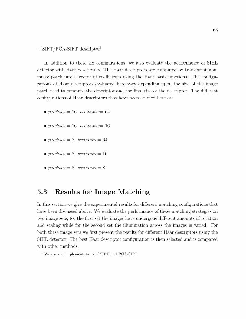
68
+ SIFT/PCA-SIFT descriptor5
In addition to these six configurations, we also evaluate the performance of SIHL
detector with Haar descriptors. The Haar descriptors are computed by transforming an
image patch into a vector of coefficients using the Haar basis functions. The configu-
rations of Haar descriptors evaluated here vary depending upon the size of the image
patch used to compute the descriptor and the final size of the descriptor. The different
configurations of Haar descriptors that have been studied here are
• patchsize= 16 vectorsize= 64
• patchsize= 16 vectorsize= 16
• patchsize= 8 vectorsize= 64
• patchsize= 8 vectorsize= 16
• patchsize= 8 vectorsize= 8
5.3 Results for Image Matching
In this section we give the experimental results for different matching configurations that
have been discussed above. We evaluate the performance of these matching strategies on
two image sets; for the first set the images have undergone different amounts of rotation
and scaling while for the second set the illumination across the images is varied. For
both these image sets we first present the results for different Haar descriptors using the
SIHL detector. The best Haar descriptor configuration is then selected and is compared
with other methods.
5We use our implementations of SIFT and PCA-SIFT

69
5.3.1 Scaling and Rotation Dataset
Haar Descriptor Evaluation
Figure 5.1 shows the matching score and the number of correct matches obtained using
different Haar descriptors for the scaling and rotation image dataset (refer to Figure
3.6). The matching score and correct matches are computed for pair of images where
one image is always the reference image (image having a scale of 1) while the second
image is another image from the dataset. The results obtained for pair of images are
shown using the scale factor parameter. The scale parameter corresponds to the scale
ratio between an image and the reference image.
In general, as the scale factor between the images increases, fewer matches are classi-
fied as correct matches. One of things that can be easily observed from the two graphs is
that the scores obtained using the first four configurations are relatively close. The last
configuration which computes an 8 bit descriptor gives comparatively poor results. This
is due to the fact that the size of the descriptor is too small to reliably distinguish image
structures. Still the number of matches obtained might suffice for some applications at
the cost of a comparatively large number of false matches.
Another observation that can be made from the results is that the size of the patch
has little effect on the number of correct matches. This is easily visible from the graph of
correct matches, where the first and third configuration (patchsize 16 and 8 respectively
for a vector size of 64) and the second and fourth configuration (patchsize 16 and 8
respectively for a vector size of 16) give almost the same number of matches. Hence,
the conclusion drawn from these two graphs is that the 64 bit Haar descriptors produce
more matches because the descriptors are more distinctive.
In order to better understand these results we study the recall vs 1-precision curves
for the same experiment. Figure 5.2 shows the recall vs 1- precision graphs for the first
and fifth image in this dataset (refer to Figure 3.6(a) and 3.6(e)). The graphs have been
obtained for nearest neighbor matching measure and distance ratio matching measure. In
distance ratio matching, the distance ratio of the nearest to the second nearest neighbor
is used to decide a match. The matching thresholds used for nearest neighbor matching
and distance ratio matching have been varied to generate their respective curves. The
conclusions drawn from the previous graphs are also evident here as the 64 bit descriptors
obtain a higher recall for the same value of 1-precision than the 16 bit descriptors. The
8 bit descriptor shows a relatively poor curve which indicates that the descriptor is not
suitable for matching. Also, all the recall vs 1-precision curves are marginally better for

70
1 1.5 2 2.5 3 3.5 4 4.50
10
20
30
40
50
60
scale factor
mat
chin
g s
core
%
Haar−patchsize16−vectorsize64Haar−patchsize16−vectorsize16Haar−patchsize8−vectorsize64Haar−patchsize8−vectorsize16Haar−patchsize8−vectorsize8
(a)
1 1.5 2 2.5 3 3.5 4 4.50
200
400
600
800
1000
1200
1400
scale factorn
o. o
f co
rrec
t m
atch
es
Haar−patchsize16−vectorsize64Haar−patchsize16−vectorsize16Haar−patchsize8−vectorsize64Haar−patchsize8−vectorsize16Haar−patchsize8−vectorsize8
(b)
Figure 5.1: Performance evaluation curves for different Haar descriptors combined with
SIHL detector for scaling and rotation image dataset (see Figure 3.6) (a) Matching Score
(b) Number of correct matches using nearest neighbor matching
0 0.1 0.2 0.3 0.4 0.5 0.6 0.7 0.8 0.9 10
0.1
0.2
0.3
0.4
0.5
0.6
0.7
0.8
0.9
1
1−precision
reca
ll
Haar−patchsize16−vectorsize64Haar−patchsize16−vectorsize16Haar−patchsize8−vectorsize64Haar−patchsize8−vectorsize16Haar−patchsize8−vectorsize8
(a)
0 0.1 0.2 0.3 0.4 0.5 0.6 0.7 0.8 0.9 10
0.1
0.2
0.3
0.4
0.5
0.6
0.7
0.8
0.9
1
1−precision
reca
ll
Haar−patchsize16−vectorsize64Haar−patchsize16−vectorsize16Haar−patchsize8−vectorsize64Haar−patchsize8−vectorsize16Haar−patchsize8−vectorsize8
(b)
Figure 5.2: Comparison of different Haar descriptors combined with SIHL detector for
two images from the scaling and rotation image dataset (see Figure 3.6(a) and 3.6(e))
(a) Nearest neighbor matching measure (b) Distance ratio matching measure
71
nearest neighbor matching than for distance ratio matching indicating nearest neighbor
matching is a slightly better similarity measure for Haar descriptors.
SIFT, PCA-SIFT Descriptor Evaluation
This section gives a comparative analysis of three detectors that have been discussed in
this research. We have chosen the 64 bit Haar descriptor of patchsize 16 as the best Haar
descriptor from the previous section. The objective is to find the best matching strategy
amongst all the different configurations. Figure 5.3 shows the graphs for matching score
and number of correct matches for all the different configurations. In order to better
understand these curves we also give the repeatability results for this image dataset from
chapter three here. The first observation that can be made from these graphs is that for
every feature detector, a better score is obtained (both in terms of matching score and
no. of correct matches) when the detector is combined with SIFT descriptor than PCA-
SIFT. This leads to the conclusion that SIFT is a better descriptor than PCA-SIFT.
This comes as no surprise as the careful design of SIFT which includes operations like
trilinear interpolation for distributing values in adjacent bins make the descriptor more
robust to localization errors than PCA-SIFT.
If we consider the three different configurations for the SIFT descriptor, the results
obtained pretty much follow the results obtained from the repeatability graph. The
SIHL detector gives the maximum number of correct matches and the highest matching
score when combined with the SIFT descriptor. For the first image, this detector gives
fewer correct matches than HL detector in spite of having more correspondences due
to repeatability. This indicates that the points detected using our detector are not as
distinct. A similar pattern can be observed when the three detectors combined with
PCA-SIFT descriptor are considered. In this case, the SIHL detector along with PCA-
SIFT gives the highest number of correct matches. Surprisingly, the 64 Haar descriptor
obtains the second highest matching score and the second largest number of matches
throughout the range of scales for the given image scene. This indicates that once a
patch has been selected around a point which is invariant to scale change and image
rotation, even a simple operation like Haar decomposition can be used to generate a
sufficiently reliable descriptor. Amongst all the different matching strategies that have
been shown, the lowest matching score is obtained for the DOG detector when combined
with PCA-SIFT descriptor.
Although these curves do indicate how good a matching technique is in finding the
number of correct matches, it tells us nothing about the number of false matches obtained.

72
1 1.5 2 2.5 3 3.5 4 4.50
10
20
30
40
50
60
70
80
90
100
scale factor
rep
eata
bili
ty %
DOGHLSIHL
(a)
1 1.5 2 2.5 3 3.5 4 4.50
200
400
600
800
1000
1200
1400
1600
1800
scale factor
no
. of
corr
esp
on
den
ces
DOGHLSIHL
(b)
1 1.5 2 2.5 3 3.5 4 4.50
10
20
30
40
50
60
scale factor
mat
chin
g s
core
%
DOG+SIFTDOG+PCA−SIFTHL+SIFTHL+PCA−SIFTSIHL+SIFTSIHL+PCA−SIFTSIHL+Haar−patchsize16−vectorsize64
(c)
1 1.5 2 2.5 3 3.5 4 4.50
200
400
600
800
1000
1200
1400
scale factor
no
. of
corr
ect
mat
ches
DOG+SIFTDOG+PCA−SIFTHL+SIFTHL+PCA−SIFTSIHL+SIFTSIHL+PCA−SIFTSIHL+Haar−patchsize16−vectorsize64
(d)
Figure 5.3: Results for different matching strategies for the scaling and rotation image
dataset (see Figure 3.6) (a) Repeatability score (b) Number of correspondences using
repeatability (c) Matching score (d) Number of correct matches
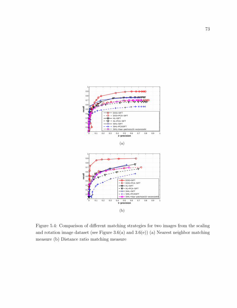
73
0 0.1 0.2 0.3 0.4 0.5 0.6 0.7 0.8 0.9 10
0.1
0.2
0.3
0.4
0.5
0.6
0.7
0.8
0.9
1
1−precision
reca
ll
DOG+SIFTDOG+PCA−SIFTHL+SIFTHL+PCA−SIFTSIHL+SIFTSIHL+PCASIFTSIHL+Haar−patchsize16−vectorsize64
(a)
0 0.1 0.2 0.3 0.4 0.5 0.6 0.7 0.8 0.9 10
0.1
0.2
0.3
0.4
0.5
0.6
0.7
0.8
0.9
1
1−precision
reca
ll
DOG+SIFTDOG+PCA−SIFTHL+SIFTHL+PCA−SIFTSIHL+SIFTSIHL+PCASIFTSIHL+Haar−patchsize16−vectorsize64
(b)
Figure 5.4: Comparison of different matching strategies for two images from the scaling
and rotation image dataset (see Figure 3.6(a) and 3.6(e)) (a) Nearest neighbor matching
measure (b) Distance ratio matching measure

74
In order to investigate that aspect, we look at the recall vs 1-precision curves of different
strategies for both nearest neighbor matching and distance ratio matching measure (refer
to Figure 5.4). The graphs have been plotted for the first and fifth image from the dataset
(refer to Figure 3.6(a) and 3.6(e)). A quick look at the these curves indicates that even
though the DOG detector with SIFT descriptor doesn’t give the highest number of
matches, it still gives the most stable matches with the fewest mismatches. This is due
to the distinctiveness of DOG points which results in very few ambiguous matches (point
in one image being matched to two or more points in the other). The curves obtained
for the two Hessian-Laplace detectors with the SIFT descriptor are quite similar. The
combination of Haar descriptor and SIHL detector and the combination DOG detector
and PCA-SIFT descriptor also give good curves. The lowest performance is obtained
when PCA-SIFT descriptor is combined with SIHL detector.
Another thing that can be observed from the two graphs is that the SIFT descriptor
obtains a higher recall for the same 1-precision value for the ratio matching measure while
the PCA-SIFT descriptor obtains a higher recall for the same 1-precision for the nearest
neighbor measure. This implies that while matching SIFT descriptors, it is better to use
the distance ratio matching measure and for PCA-SIFT, better results will be obtained
for nearest neighbor matching.
In order to summarize the results for this section; we obtain the maximum number of
correct matches for the SIHL detector combined with the SIFT descriptor. However, here
we know the ground truth between images and thus it is easier to remove false matches.
In practical applications where the mapping between two images in not known and the
objective is to get the best set of matches with the least number of false matches, the
most reliable matching strategy is the DOG detector combined with the SIFT descriptor.
Complexity Analysis: Table 5.1 below shows the time taken to compute different
descriptors using our implementations. From this table it can be concluded that it is
faster to compute Haar descriptors than SIFT and PCA-SIFT descriptors. It is important
to note these implementations are non-optimized versions and faster ways to compute
descriptors like SIFT and PCA-SIFT are already available.6 Also the times shown in
the table below will vary depending upon the number of points for which descriptors are
computed.
6SIFT:http://www.cs.ubc.ca/ lowe/keypoints/PCA-SIFT:http://www.cs.cmu.edu/ yke/pcasift/
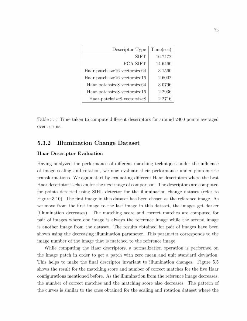
75
Descriptor Type Time(sec)
SIFT 16.7472
PCA-SIFT 14.6460
Haar-patchsize16-vectorsize64 3.1560
Haar-patchsize16-vectorsize16 2.6002
Haar-patchsize8-vectorsize64 3.0796
Haar-patchsize8-vectorsize16 2.2936
Haar-patchsize8-vectorsize8 2.2716
Table 5.1: Time taken to compute different descriptors for around 2400 points averaged
over 5 runs.
5.3.2 Illumination Change Dataset
Haar Descriptor Evaluation
Having analyzed the performance of different matching techniques under the influence
of image scaling and rotation, we now evaluate their performance under photometric
transformations. We again start by evaluating different Haar descriptors where the best
Haar descriptor is chosen for the next stage of comparison. The descriptors are computed
for points detected using SIHL detector for the illumination change dataset (refer to
Figure 3.10). The first image in this dataset has been chosen as the reference image. As
we move from the first image to the last image in this dataset, the images get darker
(illumination decreases). The matching score and correct matches are computed for
pair of images where one image is always the reference image while the second image
is another image from the dataset. The results obtained for pair of images have been
shown using the decreasing illumination parameter. This parameter corresponds to the
image number of the image that is matched to the reference image.
While computing the Haar descriptors, a normalization operation is performed on
the image patch in order to get a patch with zero mean and unit standard deviation.
This helps to make the final descriptor invariant to illumination changes. Figure 5.5
shows the result for the matching score and number of correct matches for the five Haar
configurations mentioned before. As the illumination from the reference image decreases,
the number of correct matches and the matching score also decreases. The pattern of
the curves is similar to the ones obtained for the scaling and rotation dataset where the

76
64 bit descriptors obtained the best performance followed by the 16 bit descriptors. The
8 bit descriptor gives lowest score due to poor distinctiveness.
Figure 5.6 shows the recall vs 1-precision curves plotted for an image pair (refer
to Figure 3.10(a) and 3.10(b)). The 8 bit descriptor shows a much better recall vs 1-
precision curve than what was obtained using the scaling and rotation dataset. The
reason is that it is much easier to match images which a slight illumination change than
to match images with a scale change. The best performance is again obtained by the 64
bit Haar descriptors followed by 16 bit descriptors. The size of the patch again has very
little affect on the performance of descriptors.
2 3 4 5 60
10
20
30
40
50
60
decreasing illumination
mat
chin
g s
core
%
Haar−patchsize16−vectorsize64Haar−patchsize16−vectorsize16Haar−patchsize8−vectorsize64Haar−patchsize8−vectorsize16Haar−patchsize8−vectorsize8
(a)
2 3 4 5 6100
200
300
400
500
600
700
decreasing illumination
no
. of
corr
ect
mat
ches
Haar−patchsize16−vectorsize64Haar−patchsize16−vectorsize16Haar−patchsize8−vectorsize64Haar−patchsize8−vectorsize16Haar−patchsize8−vectorsize8
(b)
Figure 5.5: Performance evaluation curves for different Haar descriptors combined with
SIHL detector for illumination change image dataset (see Figure 3.10) (a) Matching Score
(b) Number of correct matches using nearest neighbor matching
SIFT, PCA-SIFT Descriptor Evaluation
Here we compare the different matching strategies discussed before for images with illu-
mination change. Figure 5.7 shows the graphs for the matching score and the number
of correct matches obtained. The repeatability results have also been shown in order
to better interpret the matching results. For every feature detector, better results are
obtained with the SIFT descriptor than the PCA-SIFT descriptor. The HL detector
obtains the maximum number of correct matches and matching score throughout as sug-
gested from the repeatability graphs. In spite of higher repeatability than DOG detector,
we obtain fewer matches for our SIHL approach. The reason is that the regions found

77
0 0.2 0.4 0.6 0.8 10
0.1
0.2
0.3
0.4
0.5
0.6
0.7
0.8
0.9
1
1−precision
reca
ll
Haar−patchsize16−vectorsize64Haar−patchsize16−vectorsize16Haar−patchsize8−vectorsize64Haar−patchsize8−vectorsize16Haar−patchsize8−vectorsize8
(a)
0 0.2 0.4 0.6 0.8 10
0.1
0.2
0.3
0.4
0.5
0.6
0.7
0.8
0.9
1
1−precision
reca
ll
Haar−patchsize16−vectorsize64Haar−patchsize16−vectorsize16Haar−patchsize8−vectorsize64Haar−patchsize8−vectorsize16Haar−patchsize8−vectorsize8
(b)
Figure 5.6: Comparison of different Haar descriptors combined with SIHL detector for
two images from the illumination change image dataset (see Figure 3.10(a) and 3.10(b))
(a) Nearest neighbor matching measure (b) Distance ratio matching measure
using SIHL detector are less distinctive, which leads to multiple matches for a point and
more mismatches. The 64 bit Haar descriptor gives the lowest match score amongst all
the methods.
In order to get an idea about the percentage of correct and false matches for these
different methods, we plot the recall vs 1-precision curves for the first two images in this
sequence (Figure 3.10(a) and 3.10(b)). The curves are again plotted for both nearest
neighbor matching technique and the distance ratio matching technique (refer Figure
5.8). The thresholds for both these measures have been varied to plot their respective
curves. The high values of recall obtained for all curves indicates that fewer mismatches
are obtained when matching images with lighting change than matching ones with scale
change. Once again even though DOG detector gave lower repeatability scores and
fewer matches than the HL approach, it gives the best recall vs 1-precision curves. For
distance ratio matching, the best results are obtained with SIFT descriptor while for
nearest neighbor matching PCA-SIFT performs slightly better.
Hence in conclusion, the maximum number of matches are obtained by the HL de-
tector when combined with the SIFT descriptor. Still the combination of DOG detector
and SIFT descriptor performs best when it comes to giving the maximum number of
matches with the lowest false matches.

78
2 3 4 5 60
10
20
30
40
50
60
70
80
90
100
decreasing illumination
rep
eata
bili
ty %
DOGHLSIHL
(a)
2 3 4 5 60
100
200
300
400
500
600
700
800
900
1000
decreasing illumination
no
. of
corr
esp
on
den
ces
DOGHLSIHL
(b)
1.5 2 2.5 3 3.5 4 4.5 5 5.5 6 6.50
10
20
30
40
50
60
70
80
decreasing illumination
mat
chin
g s
core
%
DOG+SIFTDOG+PCA−SIFTHL+SIFTHL+PCA−SIFTSIHL+SIFTSIHL+PCA−SIFTSIHL+Haar−patchsize16−vectorsize64
(c)
1.5 2 2.5 3 3.5 4 4.5 5 5.5 6 6.50
100
200
300
400
500
600
700
800
900
decreasing illumination
no
. of
corr
ect
mat
ches
DOG+SIFTDOG+PCA−SIFTHL+SIFTHL+PCA−SIFTSIHL+SIFTSIHL+PCA−SIFTSIHL+Haar−patchsize16−vectorsize64
(d)
Figure 5.7: Results for different matching strategies for the illumination change image
dataset (see Figure 3.10) (a) Repeatability score (b) Number of correspondences using
repeatability (c) Matching score (d) Number of correct matches

79
0 0.2 0.4 0.6 0.8 10
0.1
0.2
0.3
0.4
0.5
0.6
0.7
0.8
0.9
1
1−precision
reca
ll
DOG+SIFTDOG+PCA−SIFTHL+SIFTHL+PCA−SIFTSIHL+SIFTSIHL+PCA−SIFTSIHL+Haar−patchsize16−vectorsize64
(a)
0 0.2 0.4 0.6 0.8 10.1
0.2
0.3
0.4
0.5
0.6
0.7
0.8
0.9
1
1−precision
reca
ll
DOG+SIFTDOG+PCA−SIFTHL+SIFTHL+PCA−SIFTSIHL+SIFTSIHL+PCA−SIFTSIHL+Haar−patchsize16−vectorsize64
(b)
Figure 5.8: Comparison of different matching strategies for two images from the illu-
mination change image dataset (see Figure 3.10(a) and 3.10(b)) (a) Nearest neighbor
matching measure (b) Distance ratio matching measure
80
5.4 Image Retrieval
Image retrieval can be described as the task of finding an image or a set of images closest
to the query image from a database7. Such images contain image structures which are
similar to that of a query image. Vision systems rely on extracting information from
the image content to perform image retrieval. One of the most widely used methods
of representing image content is by extracting features. Once the features have been
extracted for all the images in a database, the descriptors computed for features in the
query image can be matched across the entire database to identify images which have
similar image structure. Thus, an image retrieval system takes a given query and returns
a set of images in an order of similarity, from the image database that best matches that
query. Usually, additional constraints are applied in retrieval applications in order to
reject false feature matches.
Most of the commonly used image retrieval systems use features based on color,
texture or shape to perform retrieval. Various papers in the literature have compared
the advantages and disadvantages of using different features for performing retrieval[29,
1997][52, 1997]. Color based image retrieval is usually carried out by identifying images
which have histograms similar to the query image. Histograms are compared by either
computing their intersection[69, 1991] or by using a spatial matching function[68, 1996].
Other methods used to perform color based retrieval have been proposed where descrip-
tors have been computed from different image regions[13, 1997] or by clustering similar
color regions[17, 2001]. It has been shown that these methods are computationally more
efficient than traditional histogram methods.
Texture is an important characteristic that can be used to retrieve images. It is espe-
cially useful in scenarios where two images might look similar based on color information
but may be belong to completely different scenes(for eg. images depicting an ocean and
the sky). Tamura et al[70, 1978] proposed a method to compute six image texture fea-
tures which approximate human perception. Psychological and empirical tests were done
7Here we talk about image retrieval in the sense where the objective is to look for images whichhave the same image structures as the query image. For example, if our query image has a red ball andwe would like to find all other images which have the same red ball. The more generic form of imageretrieval deals with identifying objects from a particular category. For example, searching for all imageswhich contain pictures of cars. Such a task cannot yet be performed reliably by computer vision systemsin current practice. Image retrieval is performed for the generic case by annotating images where thesystem retrieves all the images which have the queried keyword. This method is used for retrievingimages on all internet search engines.
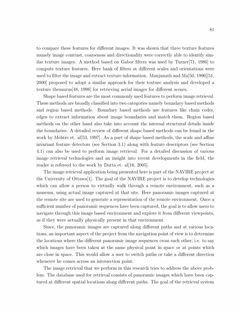
81
to compare these features for different images. It was shown that three texture features
namely image contrast, coarseness and directionality were correctly able to identify sim-
ilar texture images. A method based on Gabor filters was used by Turner[71, 1986] to
compute texture features. Here bank of filters at different scales and orientations were
used to filter the image and extract texture information. Manjunath and Ma[50, 1996][51,
2000] proposed to adopt a similar approach for their texture analysis and developed a
texture thesaurus[48, 1998] for retrieving aerial images for different scenes.
Shape based features are the most commonly used features to perform image retrieval.
These methods are broadly classified into two categories namely boundary based methods
and region based methods. Boundary based methods use features like chain codes,
edges to extract information about image boundaries and match them. Region based
methods on the other hand also take into account the internal structural details inside
the boundaries. A detailed review of different shape based methods can be found in the
work by Mehtre et. al[53, 1997]. As a part of shape based methods, the scale and affine
invariant feature detectors (see Section 3.1) along with feature descriptors (see Section
4.1) can also be used to perform image retrieval. For a detailed discussion of various
image retrieval technologies and an insight into recent developments in the field, the
reader is refereed to the work by Datta et. al[16, 2005].
The image retrieval application being presented here is part of the NAVIRE project at
the University of Ottawa[1]. The goal of the NAVIRE project is to develop technologies
which can allow a person to virtually walk through a remote environment, such as a
museum, using actual image captured at that site. Here panoramic images captured at
the remote site are used to generate a representation of the remote environment. Once a
sufficient number of panoramic sequences have been captured, the goal is to allow users to
navigate through this image based environment and explore it from different viewpoints,
as if they were actually physically present in that environment.
Since, the panoramic images are captured along different paths and at various loca-
tions, an important aspect of the project from the navigation point of view is to determine
the locations where the different panoramic image sequences cross each other; i.e. to say
which images have been taken at the same physical point in space or at points which
are close in space. This would allow a user to switch paths or take a different direction
whenever he comes across an intersection point.
The image retrieval that we perform in this research tries to address the above prob-
lem. The database used for retrieval consists of panoramic images which have been cap-
tured at different spatial locations along different paths. The goal of the retrieval system
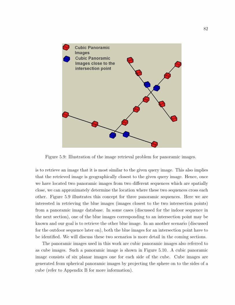
82
Figure 5.9: Illustration of the image retrieval problem for panoramic images.
is to retrieve an image that it is most similar to the given query image. This also implies
that the retrieved image is geographically closest to the given query image. Hence, once
we have located two panoramic images from two different sequences which are spatially
close, we can approximately determine the location where these two sequences cross each
other. Figure 5.9 illustrates this concept for three panoramic sequences. Here we are
interested in retrieving the blue images (images closest to the two intersection points)
from a panoramic image database. In some cases (discussed for the indoor sequence in
the next section), one of the blue images corresponding to an intersection point may be
known and our goal is to retrieve the other blue image. In an another scenario (discussed
for the outdoor sequence later on), both the blue images for an intersection point have to
be identified. We will discuss these two scenarios is more detail in the coming sections.
The panoramic images used in this work are cubic panoramic images also referred to
as cube images. Such a panoramic image is shown in Figure 5.10. A cubic panoramic
image consists of six planar images one for each side of the cube. Cube images are
generated from spherical panoramic images by projecting the sphere on to the sides of a
cube (refer to Appendix B for more information).

83
Figure 5.10: Cubic Panoramic Image, labels indicate the six sides of the cube image
A similar approach for image retrieval in the context of cube images was also used by
Fiala and Roth[22, 2005] where the SIFT method was used to correctly identify nearest
cube images.
5.5 Results
For performing image retrieval we analyze the performance of three descriptors with the
SIHL detector (our proposed Hessian-Laplace approach). The first descriptor tested is
the SIFT descriptor (our implementation) for its robustness and distinctiveness. Next
we test the 64 bit Haar descriptor obtained using a patchsize of 8 (termed as Haar-
patchsize8-vectorsize64 ). In the previous experiments the performance of this descriptor
was equivalent to the performance of the 64 bit descriptor with patchsize 16. We choose
the one with the smaller patchsize as it is slightly faster to compute. We also test a
Haar descriptor of length 16 obtained using patchsize 8 (termed as Haar-patchsize8-
vectorsize16 ). The objective of using this descriptor is to see if such a small descriptor
can give retrieval results which are comparable with descriptors like SIFT. We show
the results of these tests for two sequences; an indoor sequence termed the VIVA Lab
sequence and an outdoor sequence termed MacDonald sequence.
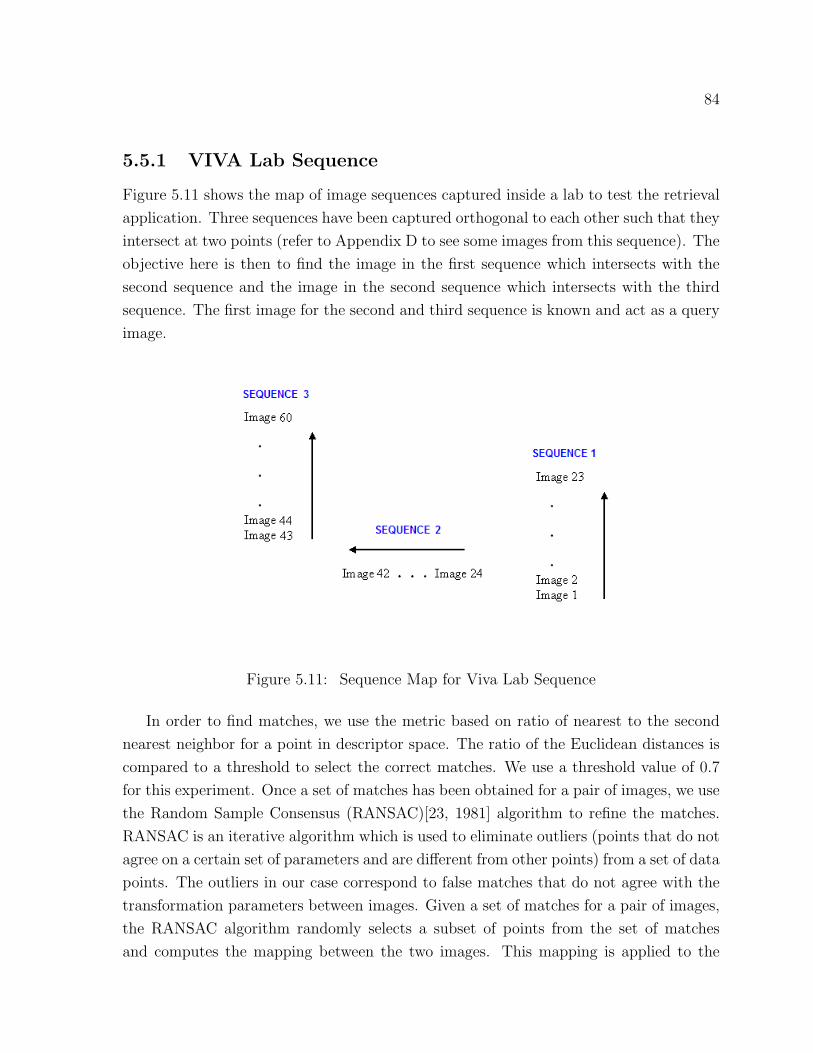
84
5.5.1 VIVA Lab Sequence
Figure 5.11 shows the map of image sequences captured inside a lab to test the retrieval
application. Three sequences have been captured orthogonal to each other such that they
intersect at two points (refer to Appendix D to see some images from this sequence). The
objective here is then to find the image in the first sequence which intersects with the
second sequence and the image in the second sequence which intersects with the third
sequence. The first image for the second and third sequence is known and act as a query
image.
Figure 5.11: Sequence Map for Viva Lab Sequence
In order to find matches, we use the metric based on ratio of nearest to the second
nearest neighbor for a point in descriptor space. The ratio of the Euclidean distances is
compared to a threshold to select the correct matches. We use a threshold value of 0.7
for this experiment. Once a set of matches has been obtained for a pair of images, we use
the Random Sample Consensus (RANSAC)[23, 1981] algorithm to refine the matches.
RANSAC is an iterative algorithm which is used to eliminate outliers (points that do not
agree on a certain set of parameters and are different from other points) from a set of data
points. The outliers in our case correspond to false matches that do not agree with the
transformation parameters between images. Given a set of matches for a pair of images,
the RANSAC algorithm randomly selects a subset of points from the set of matches
and computes the mapping between the two images. This mapping is applied to the

85
set of matches to compute the number of inliers (points which agree with the mapping)
and outliers (points that do not agree with the mapping). Recursive implementation of
this process is carried out and the mapping which gives the largest number of inliers is
selected. All the points that do not agree with this best mapping are rejected as final
outliers.
Once we have removed the false matches, the objective is to choose the image which
gives the maximum number of matches with the query image. Figure 5.12(a) shows the
result for matches obtained between cube image 24 (first image for sequence 2) and a set
of images from sequence 1. As can be seen from the results for all descriptors, high num-
ber of correspondences are obtained for images 17 and 18. The initial correspondences
obtained using the Haar descriptor are more in number than SIFT, especially for the 16
bit descriptor. This is due to the presence of similar structures in these images where the
16 bit Haar descriptor, which is less distinctive, is unable to distinguish between those
structures, which results in a large number of false matches. The number of matches
obtained with the 64 bit Haar descriptor are closer to that of SIFT.
Once RANSAC is performed, we end up with a more stable set of matches. A
closer look at the graph shows that we get more matches for image 18 with the 16 bit
Haar descriptor and SIFT descriptor, while the 64 bit Haar descriptor gives slightly
more matches (3 to be precise) for image 17. This indicates that both these images are
spatially closer to image 24 than other images and we can take the intersection point
either to be at 17 or 18. We choose the intersection point to be at 18 in this case.
A similar set of curves are plotted to find the second intersection point (refer to
Figure 5.12(b)) between sequence 2 and sequence 3. Here, image 43 of sequence 3 acts as
the query image. After performing RANSAC on initial set of correspondences, image 40
obtains the highest number of matches for SIFT and 16 bit Haar descriptor while image
41 gives slightly more matches (2 to be precise) for 64 bit Haar descriptor. This again
indicates that both images 40 and 41 are the closest to the given query image and can
be taken as intersection points. We take the intersection point to be at image 40.
Table 5.2 shows the time taken by different descriptors to retrieve the closest image
for Image 24 from the above sequence. The database used to perform retrieval is built
by selecting 25 images from the three sequences. Haar descriptor of vectorsize 16 due
to its small size takes the least amount of time followed by Haar descriptor of vectorsize
64 and SIFT. It is important to note that the time used to perform retrieval will vary
depending upon the images in the database and the number of points detected for each
image.
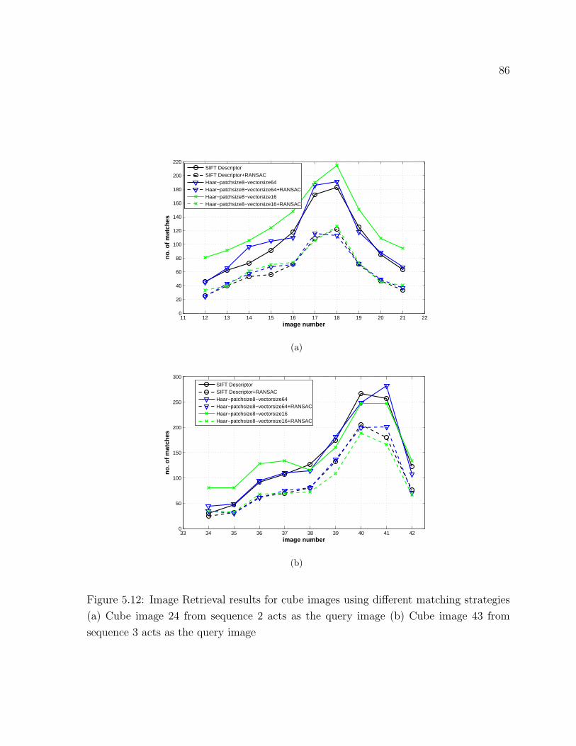
86
11 12 13 14 15 16 17 18 19 20 21 220
20
40
60
80
100
120
140
160
180
200
220
image number
no
. of
mat
ches
SIFT DescriptorSIFT Descriptor+RANSACHaar−patchsize8−vectorsize64Haar−patchsize8−vectorsize64+RANSACHaar−patchsize8−vectorsize16Haar−patchsize8−vectorsize16+RANSAC
(a)
33 34 35 36 37 38 39 40 41 420
50
100
150
200
250
300
image number
no
. of
mat
ches
SIFT DescriptorSIFT Descriptor+RANSACHaar−patchsize8−vectorsize64Haar−patchsize8−vectorsize64+RANSACHaar−patchsize8−vectorsize16Haar−patchsize8−vectorsize16+RANSAC
(b)
Figure 5.12: Image Retrieval results for cube images using different matching strategies
(a) Cube image 24 from sequence 2 acts as the query image (b) Cube image 43 from
sequence 3 acts as the query image
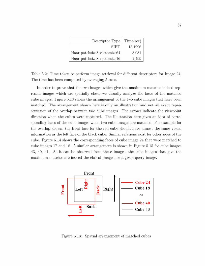
87
Descriptor Type Time(sec)
SIFT 15.1996
Haar-patchsize8-vectorsize64 8.081
Haar-patchsize8-vectorsize16 2.499
Table 5.2: Time taken to perform image retrieval for different descriptors for Image 24.
The time has been computed by averaging 5 runs.
In order to prove that the two images which give the maximum matches indeed rep-
resent images which are spatially close, we visually analyze the faces of the matched
cube images. Figure 5.13 shows the arrangement of the two cube images that have been
matched. The arrangement shown here is only an illustration and not an exact repre-
sentation of the overlap between two cube images. The arrows indicate the viewpoint
direction when the cubes were captured. The illustration here gives an idea of corre-
sponding faces of the cube images when two cube images are matched. For example for
the overlap shown, the front face for the red cube should have almost the same visual
information as the left face of the black cube. Similar relations exist for other sides of the
cube. Figure 5.14 shows the corresponding faces of cube image 24 that were matched to
cube images 17 and 18. A similar arrangement is shown in Figure 5.15 for cube images
43, 40, 41. As it can be observed from these images, the cube images that give the
maximum matches are indeed the closest images for a given query image.
Figure 5.13: Spatial arrangement of matched cubes
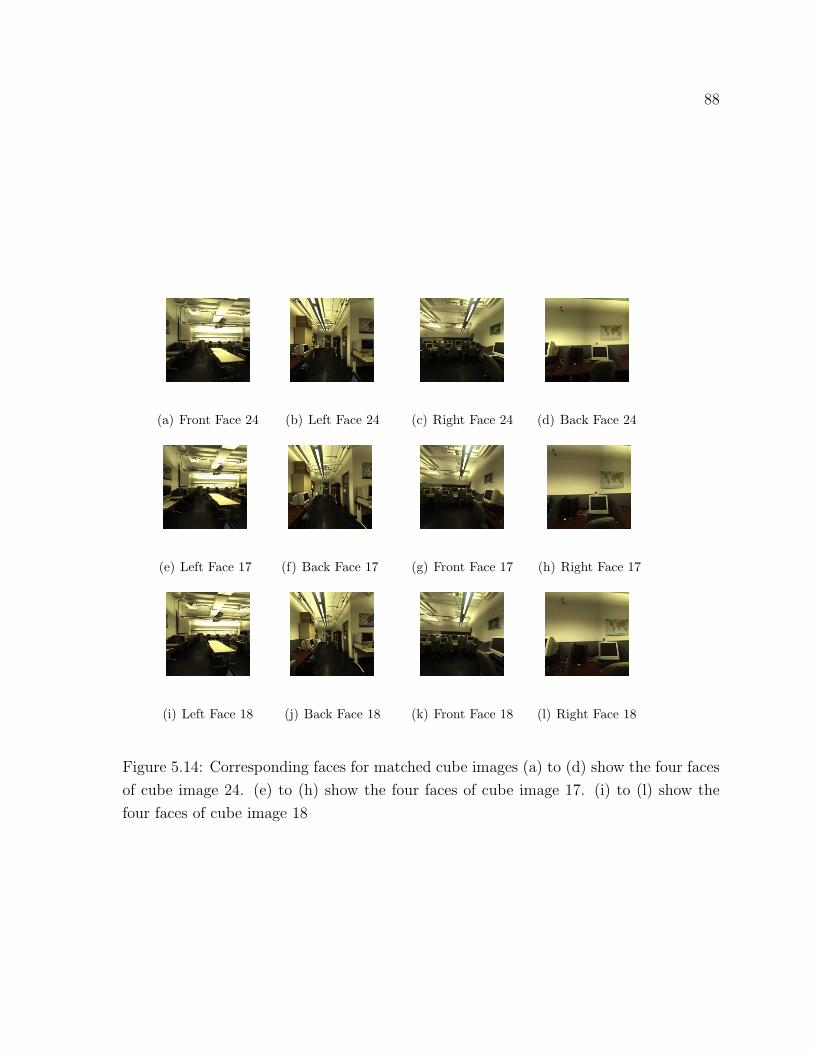
88
(a) Front Face 24 (b) Left Face 24 (c) Right Face 24 (d) Back Face 24
(e) Left Face 17 (f) Back Face 17 (g) Front Face 17 (h) Right Face 17
(i) Left Face 18 (j) Back Face 18 (k) Front Face 18 (l) Right Face 18
Figure 5.14: Corresponding faces for matched cube images (a) to (d) show the four faces
of cube image 24. (e) to (h) show the four faces of cube image 17. (i) to (l) show the
four faces of cube image 18

89
(a) Front Face 43 (b) Left Face 43 (c) Right Face 43 (d) Back Face 43
(e) Right Face 40 (f) Front Face 40 (g) Back Face 40 (h) Left Face 40
(i) Right Face 41 (j) Front Face 41 (k) Back Face 41 (l) Left Face 41
Figure 5.15: Corresponding faces for matched cube images (a) to (d) show the four faces
of cube image 43. (e) to (h) show the four faces of cube image 40. (i) to (l) show the
four faces of cube image 41

90
5.5.2 MacDonald Sequence
The indoor sequence captured before was captured under ideal conditions. This means
that the illumination was almost constant8 across the sequence and care was taken to
ensure that they were no moving objects which resulted in a large number of repeatable
points between images. It is not possible to enforce these rules for an outdoor sequence.
For outdoor sequences the images captured will always have some moving objects in the
scene. There will also be a lot of displacement of the moving objects (cars moving in
and out of the scene, people walking by). The images can also encounter illumination
changes depending upon the weather conditions. All these factors can affect the number
of matches obtained between images. However, it is hoped that the features detected
for the objects which are stationary in all images should provide enough information to
decide which images are the closest.
Another thing that can be noticed for outdoor images is that top image of the cu-
bic panorama always represents the sky. The features generated for the top image are
accidental features which are produced due to camera acquisition parameters or clouds
rather than some physical structure9. This indicates the matches obtained using the
top face are not reliable matches. Similarly the bottom image also has little relevant
information. Hence, here we exclude the features which are detected on these two faces
and use the remaining four faces for matching.
Figure 5.16 shows the map of the outdoor sequences captured10. Two small sequences
of 5 images each are captured orthogonal to each other such that they intersect at a point
(refer to Appendix D to see some images from this sequence). The distance between the
centers of the cube images is considerably larger than the distance in the indoor sequence
(cubes for outdoor sequence were captured at a distance of 3m). The objective here is to
see if the intersection point shown in the sequence map can be experimentally determined
by matching different cube images. Given a large number of sequences (each sequence
is represented by a large number of panoramic images) that cross each other, a set
of candidate images believed to be closer to an intersection point can be selected and
8The illumination may change marginally depending upon the position of camera with respect to thelight sources which are fluorescent lights
9For the indoor sequence discussed before, the lab in which the images were captured had a significantamount of structures in the top image. Hence the top image was not neglected for the previous sequence.However, if the indoor sequence is captured in a place where the ceiling is flat without any relevant imagestructures, the top image can be discarded.
10The image sequence was captured in a parking lot at a time of the day when there were few movingobjects

91
Figure 5.16: Sequence Map for MacDonald Sequence
matched to determine the actual position of the intersection point. The GPS information
for the captured images can be used to select a set of candidate images.
In order to find the intersection point for the two sequences, we treat every image
of sequence 1 as the query image and retrieve the closest image for the given query
from sequence 2. The image pair consisting of a query and retrieved image that gives the
maximum number of matches amongst all possible pairs is chosen as the pair closest to the
intersection point of the two sequences. This method of finding the closest cube images is
equivalent to matching all images from the first sequence to all the images in the second
sequence and selecting the image pair with the maximum matches. Here we compute
matches for all three configurations that have been discussed before. A distance ratio of
0.7 is used to select the correct match. Similar to the previous experiment, RANSAC is
applied to remove false matches. Here we investigate whether in all these experiments
the correct intersection point is identified.
Figure 5.17 shows the matches obtained between different images of the two sequences
for different configurations. Here we have only shown matches that have been obtained
after applying RANSAC. For all the configurations, image 5 and 7 give the maximum
number of matches followed by images 5 and 6. The matches obtained for images 4 and
7 are slightly lower than those obtained for 5 and 7. This indicates that the intersection
point should lie slightly closer to image 5 and somewhere between images 6 and 7. Hence,
as seen from the graphs, all three configurations have correctly identified the intersection
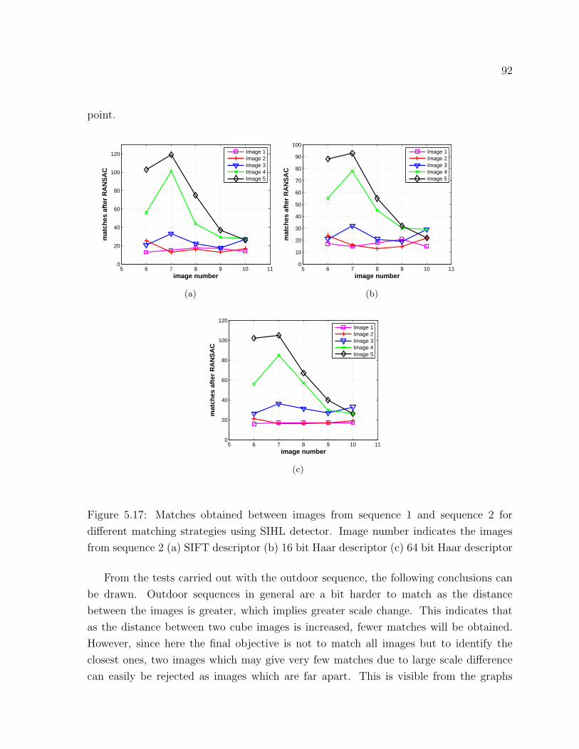
92
point.
5 6 7 8 9 10 110
20
40
60
80
100
120
image number
mat
ches
aft
er R
AN
SA
C
Image 1Image 2Image 3Image 4Image 5
(a)
5 6 7 8 9 10 110
10
20
30
40
50
60
70
80
90
100
image numberm
atch
es a
fter
RA
NS
AC
Image 1Image 2Image 3Image 4Image 5
(b)
5 6 7 8 9 10 110
20
40
60
80
100
120
image number
mat
ches
aft
er R
AN
SA
C
Image 1Image 2Image 3Image 4Image 5
(c)
Figure 5.17: Matches obtained between images from sequence 1 and sequence 2 for
different matching strategies using SIHL detector. Image number indicates the images
from sequence 2 (a) SIFT descriptor (b) 16 bit Haar descriptor (c) 64 bit Haar descriptor
From the tests carried out with the outdoor sequence, the following conclusions can
be drawn. Outdoor sequences in general are a bit harder to match as the distance
between the images is greater, which implies greater scale change. This indicates that
as the distance between two cube images is increased, fewer matches will be obtained.
However, since here the final objective is not to match all images but to identify the
closest ones, two images which may give very few matches due to large scale difference
can easily be rejected as images which are far apart. This is visible from the graphs
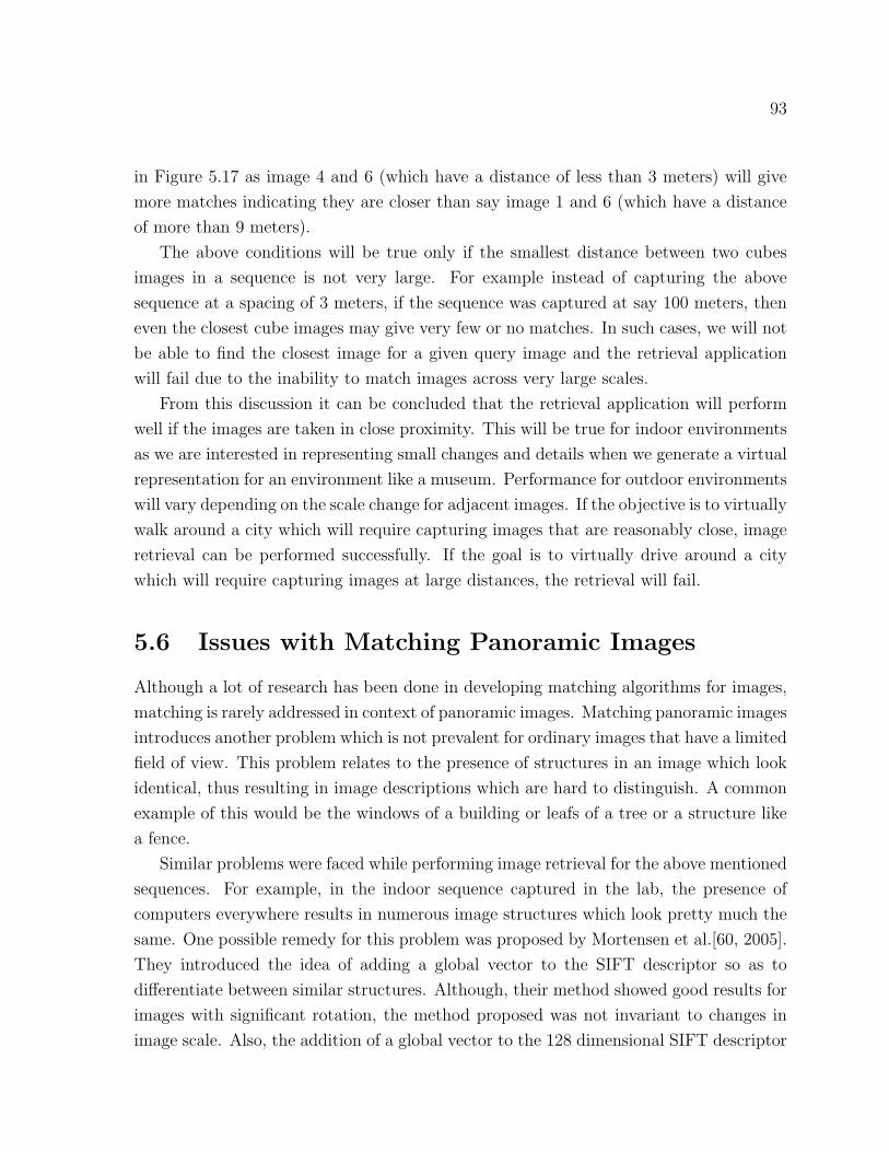
93
in Figure 5.17 as image 4 and 6 (which have a distance of less than 3 meters) will give
more matches indicating they are closer than say image 1 and 6 (which have a distance
of more than 9 meters).
The above conditions will be true only if the smallest distance between two cubes
images in a sequence is not very large. For example instead of capturing the above
sequence at a spacing of 3 meters, if the sequence was captured at say 100 meters, then
even the closest cube images may give very few or no matches. In such cases, we will not
be able to find the closest image for a given query image and the retrieval application
will fail due to the inability to match images across very large scales.
From this discussion it can be concluded that the retrieval application will perform
well if the images are taken in close proximity. This will be true for indoor environments
as we are interested in representing small changes and details when we generate a virtual
representation for an environment like a museum. Performance for outdoor environments
will vary depending on the scale change for adjacent images. If the objective is to virtually
walk around a city which will require capturing images that are reasonably close, image
retrieval can be performed successfully. If the goal is to virtually drive around a city
which will require capturing images at large distances, the retrieval will fail.
5.6 Issues with Matching Panoramic Images
Although a lot of research has been done in developing matching algorithms for images,
matching is rarely addressed in context of panoramic images. Matching panoramic images
introduces another problem which is not prevalent for ordinary images that have a limited
field of view. This problem relates to the presence of structures in an image which look
identical, thus resulting in image descriptions which are hard to distinguish. A common
example of this would be the windows of a building or leafs of a tree or a structure like
a fence.
Similar problems were faced while performing image retrieval for the above mentioned
sequences. For example, in the indoor sequence captured in the lab, the presence of
computers everywhere results in numerous image structures which look pretty much the
same. One possible remedy for this problem was proposed by Mortensen et al.[60, 2005].
They introduced the idea of adding a global vector to the SIFT descriptor so as to
differentiate between similar structures. Although, their method showed good results for
images with significant rotation, the method proposed was not invariant to changes in
image scale. Also, the addition of a global vector to the 128 dimensional SIFT descriptor

94
resulted in a large 188 dimensional feature descriptor which is time consuming to match
for recognition and retrieval applications.
Chapter 6
Conclusion
The objective of this research was to design a feature matching strategy which can find
correspondences between images that have undergone geometric and photometric trans-
formations. The feature matching technique was developed by combining two different
entities; a feature detector and a feature descriptor. A feature detector called Scale Inter-
polated Hessian-Laplace was proposed in this research and its performance was compared
with other well known detectors. Feature descriptors based on Haar wavelet transform
were introduced and compared with other descriptors in order to determine the most
robust descriptor. Finally, different matching strategies obtained using the combination
of different feature detectors and descriptors were evaluated in order to find the most
optimal matching technique.
The second part of this research addressed the issue of image retrieval for panoramic
images where the goal was to identify images which are similar to each other and spatially
close. The following sections discuss the conclusions that can be drawn from the various
tests that have been carried out in this research along with what needs to be done in
future work.
6.1 Feature Detectors
In this research we compared the performance of three feature detectors; the difference of
Gaussian (DOG) detector, the Hessian-Laplace (HL) detector proposed by Mikolajczyk
and Schmid and our version of the Hessian-Laplace detector called the Scale Interpolated
Hessian-Laplace (SIHL). The last two detectors are based on the same principle but
differ in methods used to localize points and compute orientation for points. The SIHL
95

96
detector obtained the highest repeatability score both in terms of percentage and absolute
correspondences for the scale and rotation image dataset. The HL detector gave the
highest repeatability throughout for the illumination change image dataset. Even though
the Hessian-Laplace approaches give higher repeatability scores, the points extracted by
DOG are more distinct owing to its superior localization. When points are more distinct
they give fewer ambiguous matches (point in one image being matched to two or more
points in the other). Based on just repeatability results it is difficult to decide which
detector is superior to all the others. We answer this question when we discuss matching
strategies.
6.2 Feature Descriptors
We have discussed three descriptors in this research namely SIFT descriptor, PCA-SIFT
descriptor and descriptors derived using Haar wavelet transform. The SIFT descriptor
performs best amongst all these descriptors. The SIFT descriptor is also more robust to
localization error in points than the other descriptors. The descriptors based on Haar
transform offer the advantage that they are computationally the simplest of the three.
Experimental results were given to show that these descriptors are faster to compute than
SIFT and PCA-SIFT. We have tested Haar descriptors of bit sizes 8, 16, 64 which have
been calculated from different patchsizes. Haar descriptors of length 8 owing to their size
are less distinctive and less robust. Similar problems will occur for descriptors of length
16 if the images to be matched have a lot of similar looking image structures. If the
images do not have similar looking structures, 16 bit descriptors can perform reasonably
well. Haar descriptors of length 64 can give results which are comparable with SIFT and
PCA-SIFT.
Another important issue relates to the choice of similarity metric while comparing
different descriptors. It was found that SIFT performed better when the similarity mea-
sure was distance ratio matching, while PCA-SIFT gave better performance for nearest
neighbor matching. For Haar descriptors, the performance for the two measures was
comparable with a slightly better performance obtained for nearest neighbor measure.
The choice of descriptor also depends on the application. In applications where fast
matching is required, a 128 dimensional SIFT descriptor may be too long. In such cases
PCA-SIFT and Haar descriptors are a better choice. However, in scenarios where we are
interested in obtaining very precise matches and time is not an issue, SIFT is the most
suitable descriptor.
97
6.3 Matching Strategies
Different matching configurations were explored in this research by combining different
detectors and descriptors. The objective was to identify the best matching technique
amongst all these configurations. The SIHL detector gave the largest number of matches
when combined with the SIFT descriptor for scaling and rotation image dataset. The HL
detector gave the maximum number of matches when combined with the SIFT descriptor
for the illumination change image dataset. In both cases, even though the DOG detector
with SIFT descriptor did not give the maximum number of matches, it gave the best recall
vs 1-precision curve which indicates it had the least number of false matches for a given
number of matches. This low number of false matches is due to highly distinctive points
detected with the DOG detector. Hence, we can say that the best matching strategy is
the DOG detector combined with SIFT descriptor. The matching configurations obtained
using PCA-SIFT descriptor obtained good results even though they were not as good
as SIFT descriptor. The 64 bit Haar descriptor when combined with the SIHL detector
also showed good performance both in terms of total number of matches obtained and
recall vs 1-precision curves especially for the image and rotation dataset.
6.4 Image Retrieval
We also did experiments using different matching strategies by combining our SIHL
detector with SIFT and Haar descriptors (of size 16 and 64) to perform image retrieval.
We have used a database of cubic panoramic images where we are interested in identifying
images which are similar and spatially close to a given query image. In order to do this,
we select the image which gives the maximum number of matches with the query image.
These two images which belong to two different panoramic sequences, can then be used to
determine the intersection point for the two sequences. All three configurations used in
this research were able to correctly identify the intersection point for both the indoor and
outdoor sequences. This indicates that even though Haar descriptors are less distinctive
than SIFT descriptor, they can still give enough reliable matches to identify closest
images.
98
6.5 Future Work
In this section, we give a brief overview of some the areas we would like to investigate as
part of future research.
The localization performed in this research on Hessian-Laplace points helps to localize
points efficiently in scale but not space (2D location in the image plane). We would
like to explore new ways to localize these points effectively in both scale and space
simultaneously. This should lead to more robust and distinct points.
The image retrieval tests performed in this research were carried out when they were
few moving objects in the scene and none for the indoor sequence. It would be interesting
to see if the retrieval can still be performed for a large number of moving objects and
for larger scale changes between nearest images. The sequences captured to perform
the retrieval experiments were normal to each other in order to keep the perspective
transformation between the cubes to a minimum. In future we would like to carry out
similar tests for sequences which have been taken in arbitrary directions and intersect at
arbitrary orientations. Finally, in the context of panoramic images, similar structures in
images pose a significant problem when the images have to be matched. Currently, very
little work has been done to address this problem. In future we would like to explore
different methods to disambiguate image structures without causing a significant increase
in the size of the descriptors.

Appendix A
Additional Image Matching Results
This section gives image matching results for some other image pairs1. The results have
been given in terms of recall vs 1-precision graphs.
1The image datasets were taken from http://lear.inrialpes.fr/people/mikolajczyk/
99

100
0 0.2 0.4 0.6 0.8 10
0.1
0.2
0.3
0.4
0.5
0.6
0.7
0.8
0.9
1
1−precision
reca
ll
DOG+SIFTDOG+PCA−SIFTHL+SIFTHL+PCA−SIFTSIHL+SIFTSIHL+PCA−SIFTSIHL+Haar−patchsize16−vectorsize64
(a)
0 0.2 0.4 0.6 0.8 10
0.1
0.2
0.3
0.4
0.5
0.6
0.7
0.8
0.9
1
1−precision
reca
ll
DOG+SIFTDOG+PCA−SIFTHL+SIFTHL+PCA−SIFTSIHL+SIFTSIHL+PCA−SIFTSIHL+Haar−patchsize16−vectorsize64
(b)
Figure A.1: Recall vs 1-Precision graphs for different matching strategies for the image
pair shown (a) Nearest neighbor matching measure (b) Distance ratio matching measure
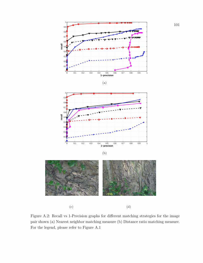
101
0 0.1 0.2 0.3 0.4 0.5 0.6 0.7 0.8 0.9 10
0.1
0.2
0.3
0.4
0.5
0.6
0.7
0.8
0.9
1
1−precision
reca
ll
(a)
0 0.1 0.2 0.3 0.4 0.5 0.6 0.7 0.8 0.9 10
0.1
0.2
0.3
0.4
0.5
0.6
0.7
0.8
0.9
1
1−precison
reca
ll
(b)
(c) (d)
Figure A.2: Recall vs 1-Precision graphs for different matching strategies for the image
pair shown (a) Nearest neighbor matching measure (b) Distance ratio matching measure.
For the legend, please refer to Figure A.1
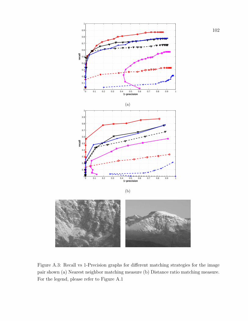
102
0 0.1 0.2 0.3 0.4 0.5 0.6 0.7 0.8 0.9 10
0.1
0.2
0.3
0.4
0.5
0.6
0.7
0.8
0.9
1
1−precision
reca
ll
(a)
0 0.1 0.2 0.3 0.4 0.5 0.6 0.7 0.8 0.9 10
0.1
0.2
0.3
0.4
0.5
0.6
0.7
0.8
0.9
1
1−precision
reca
ll
(b)
Figure A.3: Recall vs 1-Precision graphs for different matching strategies for the image
pair shown (a) Nearest neighbor matching measure (b) Distance ratio matching measure.
For the legend, please refer to Figure A.1

Appendix B
Cubic Panoramic Images
A panoramic image is an image which has a wider field of view than ordinary images.
These images can be used to generate a 360◦ representation of a scene. Mostly panoramic
images are thought of as images that have been mapped on a cylinder or a sphere. A
panoramic image format that is less frequently used is the cubic panoramic image. A
cubic panoramic image consists of six images where each image represents a side of
the cube. Since each of these six faces are planar images, cubic panoramas have less
perspective distortion as compared to other panoramic images. We now give an overview
of the method used to generate these cubic panoramas.
Figure B.1: Ladybug camera
The ladybug camera has been used here to capture the panoramic images. Figure
B.1 show the ladybug camera1. The camera consists of six 1024x768 CCD sensors; five
in a horizontal ring and one at the top. The sensors are arranged such that there is
1More information on the Ladybug camera can be found onhttp://www.ptgrey.com/products/ladybug2/index.asp
103

104
an overlap of around 80 pixels between adjacent sensors. The ladybug camera captures
information which is approximately equal to 75% of a complete sphere. Figure B.2 shows
an example of images captured using the ladybug camera inside a room.
Figure B.2: Image captured using the Ladybug camera. All the images shown have been
demosaicked
Once these images have been captured, the next step involves combining these six
images to generate a panoramic image. A spherical mesh projected on these six images
is used to generate a spherical panoramic image by mapping the images on to the mesh.
Additional blending is performed to combine regions which overlap between adjacent
images. In order to generate a cubic panoramic image from the spherical image, six
perspective views are generated from the center of the spherical image. These six views
have 90◦ field of view. Figure B.3 shows the cubic panoramic image obtained along with
its 3D rendition. Since the ladybug camera has no sensor pointing downward, the bottom
face of the cube image shows a black void which corresponds to a region for which no
information is available.
Cube images offer the advantage that they can be rendered faster using standard
graphics hardware than other formats of panoramic images[7, 2005]. We have used
the softwares written by Mark Fiala and Alan Brunton to capture ladybug images and
generate cubic panoramas. More information on how cube images are generated and
their applications can be found in works by Fiala and Roth[22, 2005], Fiala[21, 2005][20,
2005] and Bradley et al.[7, 2005]
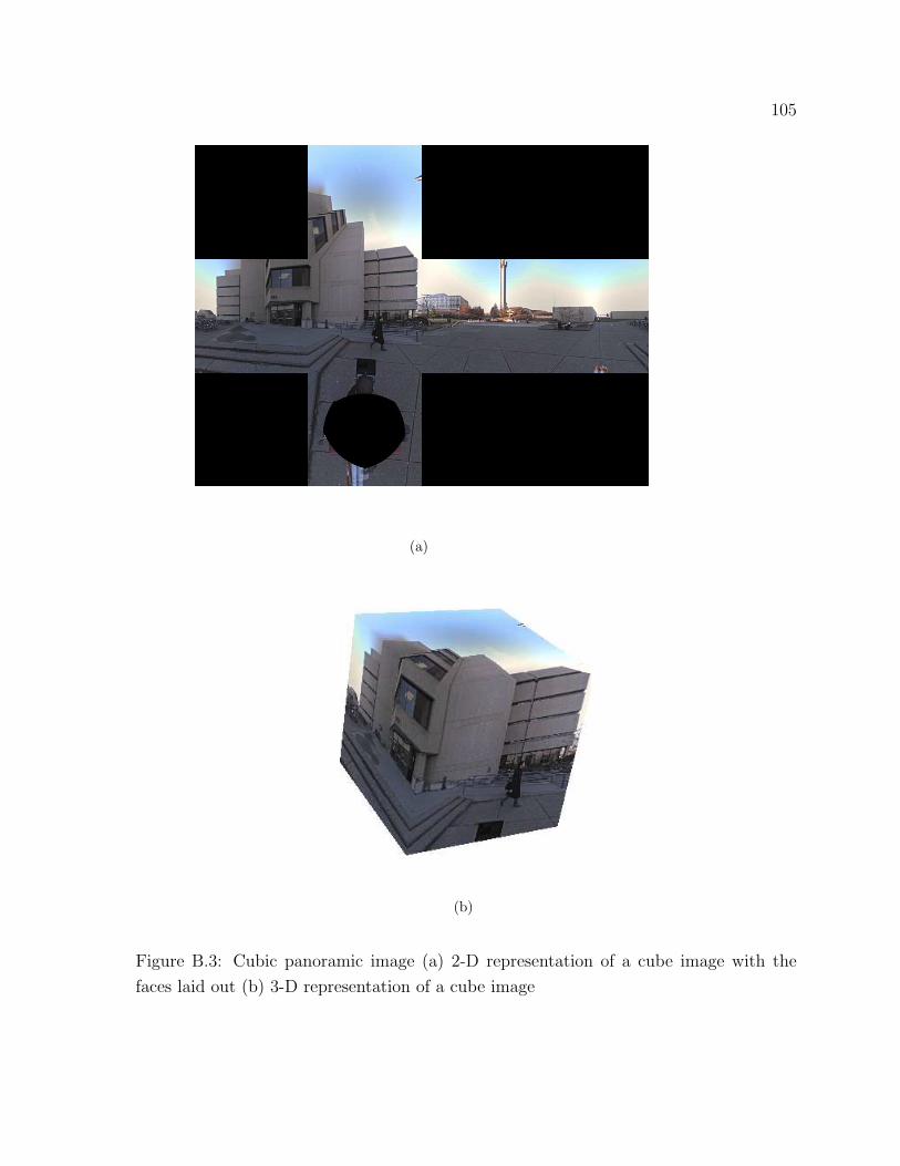
105
(a)
(b)
Figure B.3: Cubic panoramic image (a) 2-D representation of a cube image with the
faces laid out (b) 3-D representation of a cube image
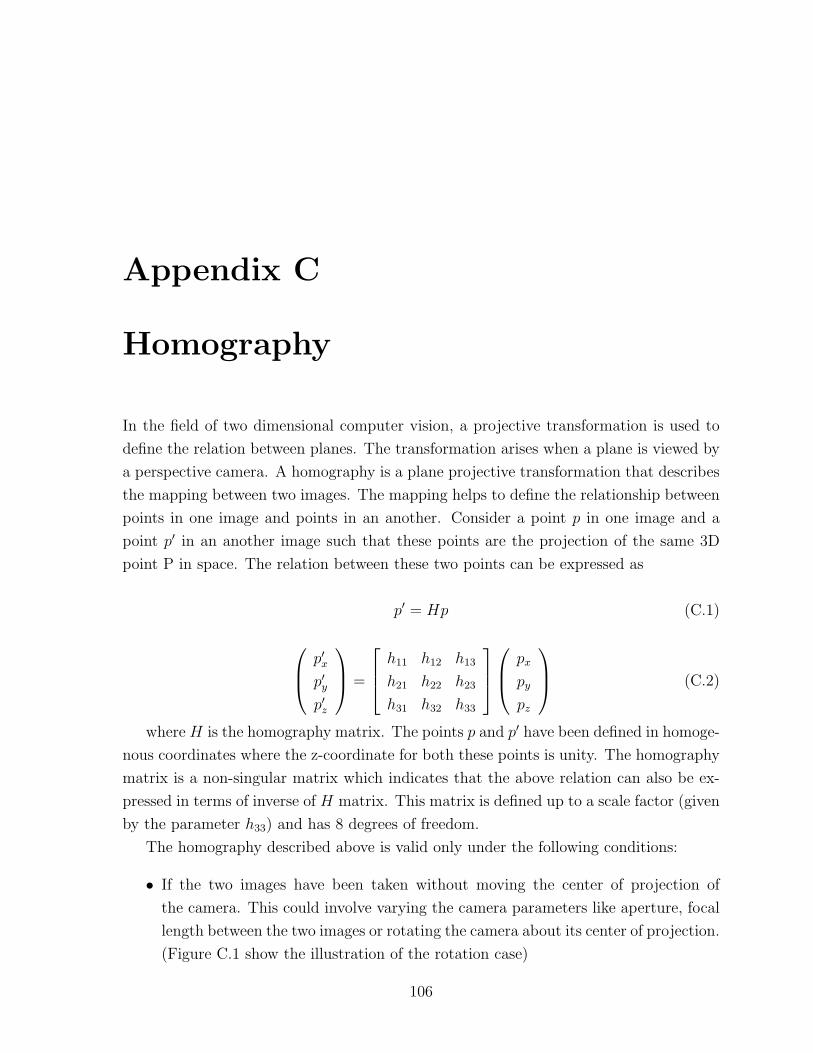
Appendix C
Homography
In the field of two dimensional computer vision, a projective transformation is used to
define the relation between planes. The transformation arises when a plane is viewed by
a perspective camera. A homography is a plane projective transformation that describes
the mapping between two images. The mapping helps to define the relationship between
points in one image and points in an another. Consider a point p in one image and a
point p′ in an another image such that these points are the projection of the same 3D
point P in space. The relation between these two points can be expressed as
p′ = Hp (C.1)
p′xp′yp′z
=
h11 h12 h13
h21 h22 h23
h31 h32 h33
px
py
pz
(C.2)
where H is the homography matrix. The points p and p′ have been defined in homoge-
nous coordinates where the z-coordinate for both these points is unity. The homography
matrix is a non-singular matrix which indicates that the above relation can also be ex-
pressed in terms of inverse of H matrix. This matrix is defined up to a scale factor (given
by the parameter h33) and has 8 degrees of freedom.
The homography described above is valid only under the following conditions:
• If the two images have been taken without moving the center of projection of
the camera. This could involve varying the camera parameters like aperture, focal
length between the two images or rotating the camera about its center of projection.
(Figure C.1 show the illustration of the rotation case)
106

107
• Both images are viewing the same planar surface from different viewpoints (Figure
C.2)
Figure C.1: The projective transformation between images taken from the same center
of projection
If the above conditions are not satisfied, parallax is introduced between images. In
such cases, the relation between two images is defined using the epipolar geometry[27,
2004]. We now discuss different methods used for computing homography. Comput-
ing the homography between images forms an essential step in camera calibration and
rectification and other applications like image mosaicing and image registration.
C.1 Computing Homography for Calibrated Cam-
eras
In this section, we describe the procedure used to compute the homography matrix for
calibrated camera setups. Before discussing this, we briefly describe the process of image
formation and give the relation between a 3D point in space and its projection on an
image plane.

108
Figure C.2: The projective transformation between two images due to a plane in 3D
space
Figure C.3 shows a camera setup (known as the pinhole camera model) consisting of
an image plane and a camera reference frame. The distance between the image plane and
the camera center C (also called center of projection) is given by the focal length (the
distance Cc in the figure). The point P is defined with respect to the camera reference
frame. The projection of point P on to the image plane is given as
p = K[I|0]P (C.3)
K =
f 0 cx
0 f cy
0 0 1
(C.4)
where p is the projection of point P and K is the camera calibration matrix defined
in terms of focal length f and center of the image plane cx and cy.
Using this basic equation, we can prove that a homography relationship holds between
two images in the case of image rotation and image scaling. For homography to be valid
for these two cases, it is essential that the camera center is stationary.

109
Figure C.3: The pinhole camera model
C.1.1 Homography for Image Scaling
In case of image scaling, the distance of the image plane from the camera reference frame
changes. This corresponds to a change in the focal length of the camera. Consider a 3D
point P and its projection p and p′ on the two images before and after scaling (zooming
in or out). Then the mapping of point P on the image planes can be expressed as
p = K[I|0]P (C.5)
p′ = K ′[I|0]P (C.6)
where K and K’ are the camera matrices. Using the above two equations, the point
p′ can be written in terms of p as
p′ = K ′K−1p (C.7)
which in turn gives
H = K ′K−1 (C.8)
Hence using the two calibration matrices, we can compute the homography between
a pair of scaled images.
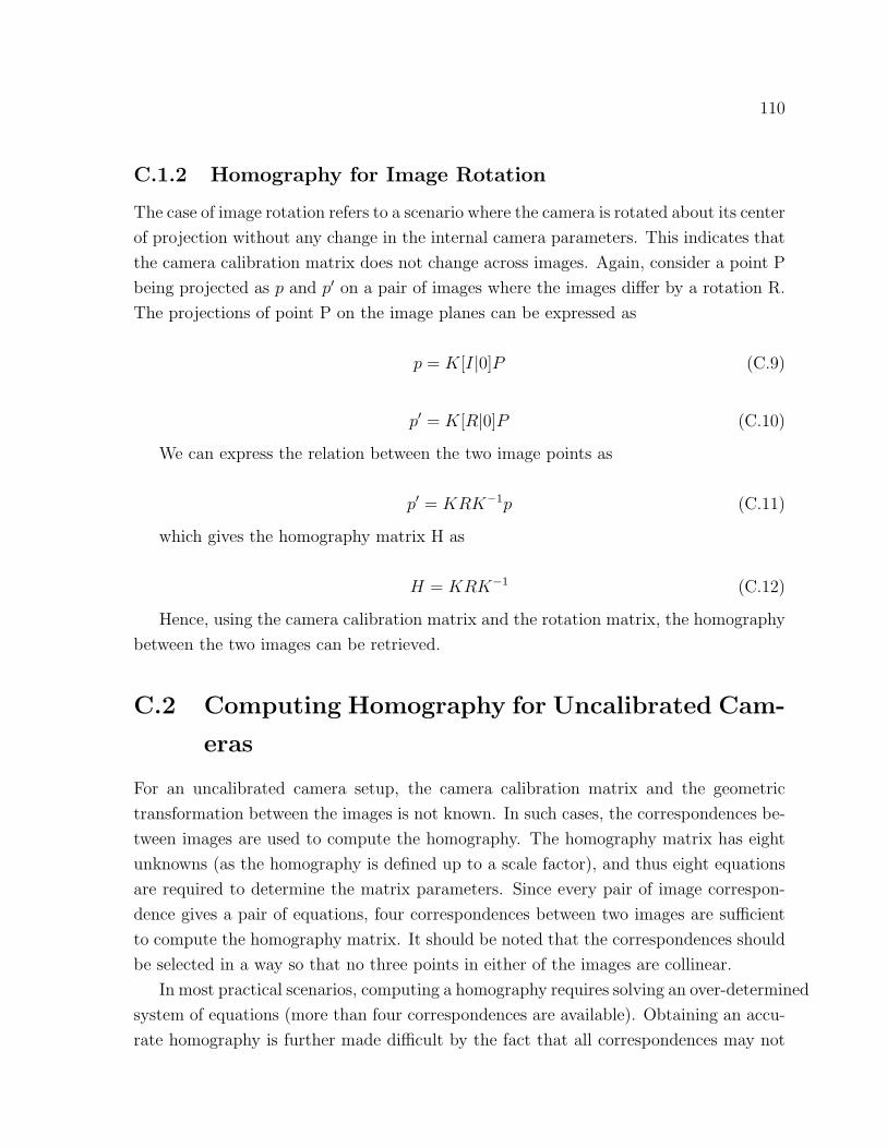
110
C.1.2 Homography for Image Rotation
The case of image rotation refers to a scenario where the camera is rotated about its center
of projection without any change in the internal camera parameters. This indicates that
the camera calibration matrix does not change across images. Again, consider a point P
being projected as p and p′ on a pair of images where the images differ by a rotation R.
The projections of point P on the image planes can be expressed as
p = K[I|0]P (C.9)
p′ = K[R|0]P (C.10)
We can express the relation between the two image points as
p′ = KRK−1p (C.11)
which gives the homography matrix H as
H = KRK−1 (C.12)
Hence, using the camera calibration matrix and the rotation matrix, the homography
between the two images can be retrieved.
C.2 Computing Homography for Uncalibrated Cam-
eras
For an uncalibrated camera setup, the camera calibration matrix and the geometric
transformation between the images is not known. In such cases, the correspondences be-
tween images are used to compute the homography. The homography matrix has eight
unknowns (as the homography is defined up to a scale factor), and thus eight equations
are required to determine the matrix parameters. Since every pair of image correspon-
dence gives a pair of equations, four correspondences between two images are sufficient
to compute the homography matrix. It should be noted that the correspondences should
be selected in a way so that no three points in either of the images are collinear.
In most practical scenarios, computing a homography requires solving an over-determined
system of equations (more than four correspondences are available). Obtaining an accu-
rate homography is further made difficult by the fact that all correspondences may not
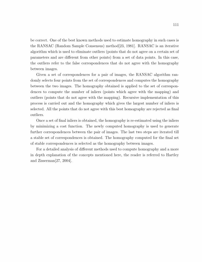
111
be correct. One of the best known methods used to estimate homography in such cases is
the RANSAC (Random Sample Consensus) method[23, 1981]. RANSAC is an iterative
algorithm which is used to eliminate outliers (points that do not agree on a certain set of
parameters and are different from other points) from a set of data points. In this case,
the outliers refer to the false correspondences that do not agree with the homography
between images.
Given a set of correspondences for a pair of images, the RANSAC algorithm ran-
domly selects four points from the set of correspondences and computes the homography
between the two images. The homography obtained is applied to the set of correspon-
dences to compute the number of inliers (points which agree with the mapping) and
outliers (points that do not agree with the mapping). Recursive implementation of this
process is carried out and the homography which gives the largest number of inliers is
selected. All the points that do not agree with this best homography are rejected as final
outliers.
Once a set of final inliers is obtained, the homography is re-estimated using the inliers
by minimizing a cost function. The newly computed homography is used to generate
further correspondences between the pair of images. The last two steps are iterated till
a stable set of correspondences is obtained. The homography computed for the final set
of stable correspondences is selected as the homography between images.
For a detailed analysis of different methods used to compute homography and a more
in depth explanation of the concepts mentioned here, the reader is referred to Hartley
and Zisserman[27, 2004].

Appendix D
Cubic Panoramic Images for Image
Retrieval
This appendix shows some of the cubic panoramic images from the indoor and outdoor
sequences used to perform image retrieval.
112
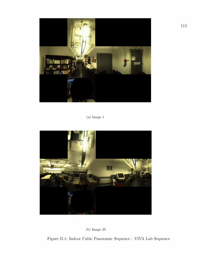
113
(a) Image 1
(b) Image 23
Figure D.1: Indoor Cubic Panoramic Sequence : VIVA Lab Sequence
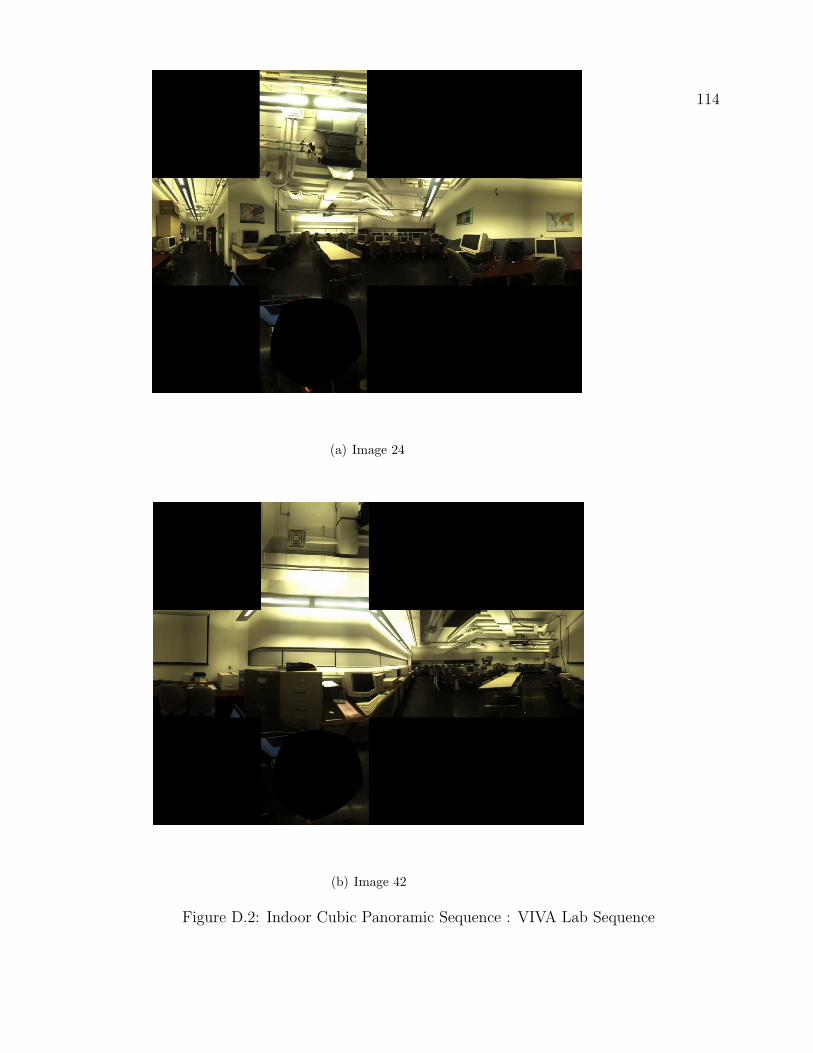
114
(a) Image 24
(b) Image 42
Figure D.2: Indoor Cubic Panoramic Sequence : VIVA Lab Sequence

115
(a) Image 1
(b) Image 5
Figure D.3: Outdoor Cubic Panoramic Sequence : MacDonald Sequence

116
(a) Image 6
(b) Image 10
Figure D.4: Outdoor Cubic Panoramic Sequence : MacDonald Sequence
Bibliography
[1] Virtual Navigation in Image-Based Representations of Real World En-
vironments (NAVIRE), VIVA Research Lab, University of Ottawa,
http://www.site.uottawa.ca/research/viva/projects/ibr/.
[2] S. Agarwal and D. Roth. Learning a Sparse Representation for Object Detection.
In Proceedings of the 7th European Conference on Computer Vision, pages 113–130,
2002.
[3] A.P. Ashbrook, N.A. Thacker, P.I Rockett, and C.I Brown. Robust Recognition of
Scale Shapes using Pairwise Geometric Histograms. In Proceedings of the 6th British
Machine Vision Conference, pages 503–512, 1995.
[4] A. Baumberg. Reliable Feature Matching across Widely Separated Views. In Pro-
ceedings of the Conference on Computer Vision and Pattern Recognition, pages 774–
781, 2000.
[5] P.R. Beaudet. Rotational Invariant Image Operators. In Proceedings of the 4th
International Conference on Pattern Recognition, pages 579–583, 1978.
[6] S. Belongie, J. Malik, and J. Puzicha. Shape Matching and Object Recognition using
Shape Contexts. IEEE Transactions on Pattern Analysis and Machine Intelligence,
24(4):509–522, 2002.
[7] D. Bradley, A. Brunton, M. Fiala, and G. Roth. Image-Based Navigation in Real
Environments using Panoramas. In IEEE International Workshop on Haptic Audio
Visual Environments and their Applications, pages 57–59, 2005.
[8] M. Brown and D.G. Lowe. Invariant Features from Interest Point Groups. In
Proceedings of the 13th British Machine Vision Conference, pages 253–262, 2002.
117

118
[9] M. Brown and D.G. Lowe. Recognising Panoramas. In Proceedings of the 9th
International Conference on Computer Vision, pages 1218–1225, October 2003.
[10] M. Brown, R. Szeliski, and S. Winder. Multi-Image Matching using Multi-Scale
Oriented Patches. In Proceedings of the Conference on Computer Vision and Pattern
Recognition, pages 510–517, 2005.
[11] M.K. Buckland and F.Gey. The relationship between Recall and Precision. Journal
of the American Society for Information Science, 45(1):12–19, 1994.
[12] P.J. Burt and E.H. Adelson. The Laplacian Pyramid as a Compact Image Code.
IEEE Transactions on Communications, 31(4):532–540, 1983.
[13] C. Carson, S. Belongie, H. Greenspan, and J. Malik. Region-Based Image Querying.
In Proceedings of IEEE Workshop on Content-Based Access of Image and Video
Libraries, pages 42–49, 1997.
[14] J.L. Crowley and A.C. Parker. A Representation for Shape based on Peaks and
Ridges in the Difference of Low Pass Transform. IEEE Transactions on Pattern
Analysis and Machine Intelligence, 6(2):156–170, 1984.
[15] J.L. Crowley, O. Riff, and J.H. Piater. Fast Computation of Characteristic Scale
using a Half-Octave Pyramid. In Cognitive Vision Workshop, 2002.
[16] R. Datta, J. Li, and J.Z. Wang. Content-Based Image Retrieval - Approaches and
Trends of the New Age. In Proceedings of the 7th ACM SIGMM International
Workshop on Multimedia Information Retrieval, pages 253–262, 2005.
[17] Y. Deng, B.S. Manjunath, C. Kenney, M.S. Moore, and H. Shin. An Efficient
Color Representation for Image Retrieval. IEEE Transactions Image Processing,
10(1):140–147, 2001.
[18] R. Deriche and G. Giraudon. Accurate Corner Detection: An Analytical Study.
In Proceedings of 3rd International Conference on Computer Vision, pages 66–70,
1990.
[19] Y. Dufournaud, C. Schmid, and R. Horaud. Matching Images with Different Reso-
lutions. In Proceedings of the Conference on Computer Vision and Pattern Recog-
nition, pages 612–618, 2000.

119
[20] M. Fiala. Immersive Panoramic Imagery. In Proceedings of the 2nd Canadian
Conference on Computer and Robot Vision, pages 386–391, 2005.
[21] M. Fiala. Pano-Presence for Teleoperation. In International Conference on Intelli-
gent Robots and Systems, pages 2170–2174, 2005.
[22] M. Fiala and G. Roth. Automatic Alignment and Graph Map Building of Panora-
mas. In IEEE International Workshop on Haptic Audio Visual Environments and
their Applications, pages 104–109, 2005.
[23] M.A. Fischler and R.C. Bolles. Random Sample Consensus: A Paradigm for Model
Fitting with Applications to Image Analysis and Automated Cartography. Commu-
nications of the ACM, 24(6):381–395, 1981.
[24] L.M.J. Florack, B.M.Ter Haar Romeny, J.J. Koenderink, and M.A. Viergever. Scale
and the Differential Structure of Images. 10(6):376–388, 1992.
[25] W.T. Freeman and E.H. Adelson. The Design and Use of Steerable Filters. IEEE
Transactions on Pattern Analysis and Machine Intelligence, 13(9):891–906, 1991.
[26] C. Harris and M. Stephens. A Combined Corner and Edge Detector. In Proceedings
of 4th Alvey Vision Conference, pages 147–151, August 1988.
[27] R. I. Hartley and A. Zisserman. Multiple View Geometry in Computer Vision.
Cambridge University Press, ISBN: 0521540518, Second edition, 2004.
[28] C. Heipke. Overview of Image Matching Techniques. In Workshop on the Application
of Digital Photogrammetric Workstations, pages 173–189, 1996.
[29] F. Idris and S. Panchanathan. Review of Image and Video Indexing Techniques.
Journal of Visual Communication and Image Representation, 8(2):146–166, 1997.
[30] A. Johnson and M. Hebert. Using Spin Images for Efficient Object Recognition in
Cluttered 3D Scenes. IEEE Transactions on Pattern Analysis and Machine Intelli-
gence, 21(5):433–449, 1999.
[31] I.T. Jolliffe. Principal Component Analysis. Springer, Second edition, 2002.
[32] T. Kadir and M. Brady. Scale Saliency and Image Description. International Journal
of Computer Vision, 45(2):83–105, 2001.
120
[33] T. Kadir, A. Zisserman, and M. Brady. An Affine Invariant Salient Region Detector.
In Proceedings of the 8th European Conference on Computer Vision, pages 228–241,
2004.
[34] Y. Ke and R. Sukthankar. PCA-SIFT: A More Distinctive Representation for Local
Image Descriptors. In Proceedings of Conference on Computer Vision and Pattern
Recognition, pages 506–513, 2004.
[35] L. Kitchen and A. Rosenfeld. Gray Level Corner Detection. Pattern Recognition
Letters, 1:95–102, December 1982.
[36] J.J. Koenderink. The Structure of Images. In Biological Cybernetics, number 5,
pages 363–370, 1984.
[37] J.J. Koenderink and A.J. Vav Doorn. Representation of Local Geometry in the
Visual System. 55(6):367–375, 1987.
[38] S. Krishnamachari and M.A. Mottaleb. Compact Color Descriptor for Fast Image
and Video Segment Retrieval. In Proceedings of IST/SPIE Conference on Storage
and Retrieval of Media Databases, 2000.
[39] S. Lazebnik, C. Schmid, and J. Ponce. A Sparse Texture Representation using
Affine-Invariant Regions. In Proceedings of the Conference on Computer Vision and
Pattern Recognition, pages 319–324, 2003.
[40] T. Lindeberg. On the Axiomatic Foundations of Linear Scale-Space: Combining
Semi-Group Structure with Causality vs. Scale Invariance. Technical report CVAP-
159, Royal Institute of Technology, Stockholm, Sweden, 1994.
[41] T. Lindeberg. Scale-Space Theory: A Basic Tool for Analysing Structures at Dif-
ferent Scales. Journal of Applied Statistics, 21(2):224–270, 1994.
[42] T. Lindeberg. Feature Detection with Automatic Scale Selection. International
Journal of Computer Vision, 30(2):77–116, 1998.
[43] T. Lindeberg and L. Bretzner. Real-Time Scale Selection in Hybrid Multi-Scale
Representations. In Proceedings of 4th International Conference on Scale-Space
Theories in Computer Vision, pages 148–163, 2003.

121
[44] T. Lindeberg and J. Garding. Shape-Adapted Smoothing in Estimation of 3-D
Shape Cues from Affine Distortions of Local 2-D Brightness Structure. Image and
Vision Computing, 15(6):415–434, 1997.
[45] H. Ling and D.W. Jacobs. Deformation Invariant Image Matching. In Proceedings
of the 10th International Conference on Computer Vision, pages 1466–1473, 2005.
[46] D.G. Lowe. Object Recognition from Local Scale Invariant Features. In Proceedings
of International Conference on Computer Vision, pages 1150–1157, 1999.
[47] D.G. Lowe. Distinctive Image Features from Scale Invariant Keypoints. Interna-
tional Journal of Computer Vision, 60(2):91–110, 2004.
[48] W.Y. Ma and B.S Manjunath. A Texture Thesaurus for Browsing Large Aerial
Photographs. Journal of the American Society for Information Science, 49(7):633–
648, 1998.
[49] P. Majer. The Influence of the γ -Parameter on Feature Detection with Automatic
Scale Selection. In 3rd International Conference, Scale-Space,number 2106 in LNCS,
pages 245–254, 2001.
[50] B.S Manjunath and W.Y. Ma. Texture Features for Browsing and Retrieval of
Image Data. IEEE Transactions on Pattern Analysis and Machine Intelligence,
18(8):837–842, 1996.
[51] B.S. Manjunath, P. Wu, S. Newsam, and H.D. Shin. A Texture Descriptor for Brows-
ing and Similarity Retrieval. Journal of Signal Processing: Image Communication,
16(1):33–43, 2000.
[52] M.De Marsicoi, L. Cinque, and S. Levialdi. Indexing Pictorial Documents by their
Content: A Survey of Current Techniques. Journal of Image and Vision Computing,
15(2):119–141, 1997.
[53] B.M. Mehtre, M.S. Kankanhalli, and W.F. Lee. Shape Measures for Content
Based Image Retrieval: A Comparison. Information Processing and Management,
33(3):319–337, 1997.
[54] K. Mikolajczyk. Detection of Local Features Invariant to Affine Transformations.
PhD thesis, INPG, Grenoble, July 2002.
122
[55] K. Mikolajczyk and C. Schmid. Indexing based on Scale Invariant Interest Points. In
Proceedings of the 8th International Conference on Computer Vision, pages 525–531,
2001.
[56] K. Mikolajczyk and C. Schmid. Scale and Affine Invariant Interest Point Detectors.
International Journal of Computer Vision, 60(1):63–86, 2004.
[57] K. Mikolajczyk and C. Schmid. A Performance Evaluation of Local Descriptors.
IEEE Transactions on Pattern Analysis and Machine Intelligence, 27(10):1615–
1630, 2005.
[58] K. Mikolajczyk, T. Tuytelaars, C. Schmid, A. Zisserman, J. Matas, F. Schaffalitzky,
T. Kadir, and L. Van Gool. A Comparison of Affine Region Detectors. International
Journal of Computer Vision, 65(1-2):43–72, 2005.
[59] H. Moravec. Towards Automatic Visual Obstacle Avoidance. In Proceedings of the
5th International Joint Conference on Artificial Intelligence, pages 584–590, August
1977.
[60] E.N. Mortensen, H. Deng, and L. Shapiro. A SIFT Descriptor with Global Con-
text. In Proceedings of the Conference on Computer Vision and Pattern Recognition,
pages 184–190, 2005.
[61] J. Niemenmaa. Feature Detection in Images with the Hybrid-Pyramid Representa-
tion: System Design, Theoretical Analysis and Experimental Evaluation. Master’s
thesis, KTH, Stockholm, Sweden, 2001.
[62] J.A. Noble. Finding Corners. Image and Vision Computing, 6(2):121–128, 1988.
[63] L. Qin and W. Gao. Image Matching based on a Local Invariant Descriptor. In
Proceedings of the International Conference on Image Processing, pages 377–380,
2005.
[64] F. Schaffalitzky and A. Zisserman. Multi-View Matching for Unordered Image Sets.
In Proceedings of the 7th European Conference on Computer Vision, pages 414–431,
2002.
[65] C. Schmid and R. Mohr. Local Grayvalue Invariants for Image Retrieval. IEEE
Transactions on Pattern Analysis and Machine Intelligence, 19(5):530–535, 1997.

123
[66] C. Schmid, R. Mohr, and C. Bauckhage. Comparing and Evaluating Interest Points.
In Proceedings of International Conference on Computer Vision, pages 230–235,
1998.
[67] E.J. Stollnitz, T.D. DeRose, and D.H. Salesin. Wavelets for Computer Graphics: A
Primer, Part 1. IEEE Computer Graphics and Applications, 3(15):76–84, 1995.
[68] M.A. Stricker and A. Dimai. Color Indexing with Weak Spatial Constraints. In
Storage and Retrieval for Image and Video Databases (SPIE), pages 29–40, 1996.
[69] M.J. Swain and D.H. Ballard. Color Indexing. International Journal of Computer
Vision, 7(1):11–32, 1991.
[70] H. Tamura, S. Mori, and T. Yamawaki. Textural Features Corresponding to Visual
Perception. IEEE Transactions in Systems Man and Cybernetics, 8(6):460–473,
1978.
[71] M. Turner. Texture Discrimination by Gabor Functions. Biological Cybernetics,
55:71–82, 1986.
[72] T. Tuytelaars and L. Van Gool. Content based Image Retrieval based on Local
Affinely Invariant Regions. In 3rd International Conference on Visual Information
Systems, pages 493–500, 1999.
[73] T. Tuytelaars and L. Van Gool. Wide Baseline Stereo Matching based on Local
Affinely Invariant Regions. In Proceedings of the 11th British Machine Vision Con-
ference, pages 412–425, 2000.
[74] A. Utenpattanant, O. Chitsobhuk, and A. Khawne. Color Descriptor for Image
Retrieval in Wavelet Domain. In Proceedings of 8th International Conference on
Advanced Communication Technology, pages 818–821, 2006.
[75] E. Vincent and R. Laganiere. Detecting and Matching Feature Points. Journal of
Visual Communication and Image Representation, 16(1):38–54, 2005.
[76] A. Witkin. Scale Space Filtering: A New Approach to Multi Scale Description.
In Proceedings of the International Conference on Acoustics, Speech, and Signal
Processing, pages 150–153, 1984.
[77] Z. Zheng, H. Wang, and E.K. Teoh. Analysis of Gray Level Corner Detection.
Pattern Recognition Letters, 20(2):149–162, 1999.