henryk svensmark: evidence of nearby supernovae affecting life on earth (arxiv. org)
TRANSCRIPT

7/28/2019 Henryk SVENSMARK: Evidence of nearby supernovae affecting life on Earth (arXiv. org)
http://slidepdf.com/reader/full/henryk-svensmark-evidence-of-nearby-supernovae-affecting-life-on-earth-arxiv 1/21
a r X i v : 1 2 1 0 . 2 9 6 3 v 1 [ a s t r o - p h . S R
] 1 0 O c t 2 0 1 2
Mon. Not. R. Astron. Soc. 000, 000–000 (0000) Printed 11 October 2012 (MN LATEX style file v2.2)
Evidence of nearby supernovae affecting life on Earth
Henrik Svensmark 1⋆1 National Space Institute, Technical University of Denmark,
Juliane Marie Vej 30, 2100 Copenhagen Ø, Denmark
11 October 2012
ABSTRACT
Observations of open star clusters in the solar neighborhood are used to calculate local super-nova (SN) rates for the past 510 million years (Myr). Peaks in the SN rates match passagesof the Sun through periods of locally increased cluster formation which could be caused byspiral arms of the Galaxy. A statistical analysis indicates that the Solar System has experi-enced many large short-term increases in the flux of Galactic cosmic rays (GCR) from nearbysupernovae. The hypothesis that a high GCR flux should coincide with cold conditions onthe Earth is borne out by comparing the general geological record of climate over the past510 million years with the fluctuating local SN rates. Surprisingly a simple combination of tectonics (long-term changes in sea level) and astrophysical activity (SN rates) largely ac-counts for the observed variations in marine biodiversity over the past 510 Myr. An inversecorrespondence between SN rates and carbon dioxide (CO2) levels is discussed in terms of apossible drawdown of CO2 by enhanced bioproductivity in oceans that are better fertilized incold conditions - a hypothesis that is not contradicted by data on the relative abundance of theheavy isotope of carbon, 13C.
Key words: Astrobiology - Earth - supernovae: general - cosmic rays - open clusters andassociations: general - Galaxy: structure
1 INTRODUCTION
That life on Earth has always been subjected to strong influences
from the cosmos has been among the main revelations in geology
in recent decades. Headlines include the verification of the plane-
tary Milankovitch effect as a pacesetter of glacial cycles, the reali-
sation that life was unsustainable during a heavy bombardment of
the young Earth (Hadean Eon), and the evidence that the Mesozoic
Era of giant reptiles ended suddenly when an asteroid hit Mex-
ico. Learning from such terrestrial examples, astrobiologists have
wondered whether cosmic hazards may make some planetary sys-
tems unsuitable for life. For example, by analogy to the Goldilocks
Zone of optimal stellar irradiation, Lineweaver et al. (2004) discuss
a Galactic habitable zone in the Milky Way where one requirementis ”an environment free of life-extinguishing supernovae”.
Even though life in general has survived robustly on our planet
for billions of years, the fossil evidence tells of continual changes
among the inhabiting species in an ever-variable climate. Ninety
years ago the astrophysicist Shapley (1921) suggested that ice ages
on the Earth might be due to the Solar System’s encounters with
gas clouds in the Milky Way. That idea was revived half a century
later by McCrea (1975), pursued by Talbot & Newman (1977) and
developed recently using better observations by Frisch (2000). But
among some of those investigating risks associated with Earth’s
interaction with the interstellar medium, interest shifted to possi-
⋆ E-mail: [email protected] (Paper accepted by MNRAS 2012 March 17)
ble climatic and biological effects of radiation from supernovae
exploding nearby. An ”ultraviolet deluge” at the Earth’s surface,
due to formation of nitrogen oxides and consequent damage to the
ozone layer, was proposed in 1974 by Ruderman (1974). Others ex-
amined the idea (Whitten et al. 1976; Gehrels et al. 2003) and even
suggested that supernovae could cause mass extinctions of living
species (Terry & Tucker 1968; Russell & Tucker 1971; Reid et al.
1978).
Consideration of the effects of nearby supernovae (SNs) has
recently focused on the influence of Galactic cosmic rays (GCR)
generated by SN remnants. As discussed more historically in Sect.
6, empirical evidence suggests that ionization of the air by GCR
has influenced the terrestrial climate on time scales ranging fromdays (Svensmark et al. 2009) to billion of years (Shaviv 2003).
Sufficiently energetic GCR primaries from SNs (>10 GeV) pro-
voke showers of secondary particles in the atmosphere that in-
clude muons which dominate at the lowest altitudes. The hypothe-
sis (Marsh & Svensmark 2000) is that ionization by the secondary
particles helps to seed the formation of low clouds, by assisting
the formation of aerosols (r ≈ 2-3 nm), some of which subse-
quently grow into cloud condensation nuclei (r larger than ≈ 50
nm). A high flux of GCR results in an increase in the number
of cloud condensation nuclei which in turn increases the albedo
of the clouds. As low clouds exert a cooling effect by increasing
the Earth’s albedo, high GCR fluxes imply low global tempera-
tures, and vice versa. The chemical mechanism that promotes the
creation of cloud condensation nuclei from sulphur compounds in
c 0000 RAS

7/28/2019 Henryk SVENSMARK: Evidence of nearby supernovae affecting life on Earth (arXiv. org)
http://slidepdf.com/reader/full/henryk-svensmark-evidence-of-nearby-supernovae-affecting-life-on-earth-arxiv 2/21
2 H. Svensmark
the air has been verified in the laboratory (Svensmark et al. 2007;
Enghoff et al. 2011; Svensmark et al. 2012), and observationally
the whole chain from GCR, to aerosols, to clouds has been ob-
served in connection with sudden solar coronal mass ejections on
time scales of days (Svensmark et al. 2009; Svensmark et al. 2012).
The energetic GCR that ionize the lower atmosphere are onlyweakly influenced by variations in the geomagnetic field or by solar
magnetic activity. Both cause low-altitude ionization rates to vary
by (≈10%) in the course of a magnetic reversal or during a solar
cycle. Over decades to millennia the GCR influx to the Solar Sys-
tem scarcely changes. On longer time scales, changes in GCR very
much larger than those due to geomagnetic or solar activity occur
as a result of variations in the rate of nearby SNs. Since the the main
ionization in the Earth’s lower atmosphere is caused by 10-20 GeV
GCR, such energies will be implicitly assumed in the following.
Fields & Ellis (1999) speculated that increased cloud cover
due to GCR from a very close SN could cause a ”cosmic ray win-
ter”. A more comprehensive scenario from Shaviv (Shaviv 2002,
2003; Shaviv & Veizer 2004) linked icy episodes on the Earth dur-
ing the 542 Myr of the Phanerozoic Eon to the Solar System’s en-counters with spiral arms of the Milky Way as it orbited around the
Galactic centre. Shaviv attributed the climatic effect to enhanced
GCR, as did de la Fuente Marcos & de la Fuente Marcos (2004) in
a study that used local star formation rates as a proxy for GCR in-
tensities. Some scientists have strongly opposed Shaviv’s scenario
and suggest that a GCR link to climate is at most of secondary im-
portance to variations in CO2 concentrations (Royer et al. 2004).
One source of difficulty in resolving this issue, which is central to
understanding Earth history during the main eon of plant and an-
imal evolution, has been uncertainties in the geological record of
climate. Recent research has improved the situation in that respect.
On the astronomical side, the Galaxy’s spiral pattern, its rotation
speed and its density variations remain uncertain. Star formation is
mainly confined to the Galaxy’s spiral arms, which are lit by mas-sive young stars. It is now generally accepted that the spiral struc-
ture seen in many galaxies is produced by density waves and prob-
ably persists for billions of years. As the Sun is a typical disk star
of the Milky Way, orbiting around the Galactic centre, an impor-
tant feature of the ever-changing environment experienced by the
Solar System is the formation of new stars from nearby gas clouds.
A large fraction of star formation in the Galaxy is accounted for by
cluster formation (Lada & Lada 2003), and the ages of clusters are
also a guide to the changing birth rate of massive stars. New stars
that are more than about 8 solar masses (M⊙) end their relatively
short lives in SN explosions. These generate the shock fronts in the
interstellar medium that are believed to accelerate GCR to ener-
gies in the range from 106 eV to 1017 eV (Berezhko & Volk 2007).
The GCR primary particles are mainly protons (≈ 91%) and nu-clei, and their energy density of 1 eV cm−3 is comparable to the
energy densities of the Galactic magnetic fields and the interstellar
gas pressure, so that GCR play an important part in the dynamics
and evolution of the interstellar medium (Boulares & Cox 1990).
In a model based on observed positions of the spiral arms,
and the relative speed of the Sun, Ω0, with respect to the pattern
speed, ΩP , of the spiral structure, Ω0 − ΩP , as estimated from
the literature, Shaviv (2002) inferred the GCR flux experienced by
the Solar System as it travelled through four spiral arms. The flux
reached a maximum after each encounter with a spiral arm, and
then went to a minimum in the dark spaces between the arms. The
interval between spiral arm visits was judged to be ≈ 140 Myr.
Unfortunately the overall structure of the Milky Way is hard to see
because of our position within the disk, and only recently has it
been generally accepted that the Galaxy possesses a central bar.
Although observations of the 21-cm hydrogen line show a four-
arm spiral structure, there are still suggestions that the Milky Way
is mainly a two-arm spiral galaxy.
In this paper the aim is to use the least model-dependent ap-
proach to the course of events in the past 500 Myr, by deriving
the star formation rates and supernova rates directly from open star
clusters in the solar neighbourhood, and using the SN rate as a
proxy for the GCR flux to the Solar System. The paper is organized
as follows. In Sect. 2 the cluster formation rates over the past 500
Myr are derived directly from open star clusters in the solar neigh-
bourhood, and then used in Sect. 3 for computing the local SN rates
as a proxy for the GCR flux to the Solar System. In addition local
features of Galactic structure are inferred from contrasting histories
in star formation outside and inside the solar circle. In a effort to
test the results in Sect. 3 a numerical model is used in 4 to simulate
the birth, dynamics and lifetimes of open clusters, and perform ex-
actly the same analysis as done with the observational data of open
clusters. To complete the astrophysics, Sect. 5 shows how a close
SN (< 300 pc) results in a short and sharp spike in the GCR flux.In Sect. 6, where attention turns to consequences of the chang-
ing GCR flux for the Earth’s climate, those spikes due to the near-
est SN events are offered as an explanation of relatively sudden
and short-lived falls in sea level, with brief glaciations causing the
marine regressions. Comparisons of SN rates with the terrestrial cli-
mate record on longer time scales confirm the match between major
periods of glaciation and persistently high GCR fluxes. Given this
evidence for large effects on climate, large impacts on life are also
to be expected. Section 7 explores an evident link between SN rates
and evolutionary history, as manifest in variations in marine biodi-
versity. Also correlating with SN rates are variations in the Earth’s
carbon cycle involving bio-productivity and (in anti-correlation)
carbon dioxide concentrations, during the past 500 Myr. Sect. 8 dis-
cusses some implications of the paper’s results, for astrophysics,palaeoclimatology and the history of life, and Sect. 9 offers brief
conclusions that focus on the empirical evidence for a large impact
of SNs on the prosperity of the Earth’s biosphere.
2 OPEN STAR CLUSTERS IN THE EARTH’S GALACTIC
VICINITY
Avoiding any preconception of the precise structure of the Galaxy
or of the Solar System’s motion through it, the present work will re-
construct the star formation in the solar neighbourhood during the
last 500 Myr from open star clusters, with a view to inferring the
local SN rate as a proxy for GCR (VERITAS Collaboration et al.
2009). It is generally believed that nearly all star formation has oc-curred in open clusters, where stars made from the same gas cloud
remain for a certain time bround together by gravitation. Within
each cluster the stars therefore have the same chemical composi-
tion and age. The Pleiades cluster for example, known since an-
cient times, is 150 pc away and estimated to be 142 Myr old, which
assigns it to the Cretaceous Period on the Earth. The justification
for using the number of open clusters as a proxy for large massive
stars is the evidence that the massive SN progenitor stars are mainly
formed in the central region of rich stellar clusters (Zinnecker et al.
1993; Hillenbrand 1997; Zinnecker & Yorke 2007). Secondly, of
the open clusters made and embedded in giant molecular clouds,
only a small fraction survive the first few million years and become
visible open clusters. This small fraction of surviving open clusters
are likely to have been the initially most rich clusters (Lada & Lada
c 0000 RAS, MNRAS 000, 000–000

7/28/2019 Henryk SVENSMARK: Evidence of nearby supernovae affecting life on Earth (arXiv. org)
http://slidepdf.com/reader/full/henryk-svensmark-evidence-of-nearby-supernovae-affecting-life-on-earth-arxiv 3/21
Evidence of nearby supernovae affecting life on Earth 3
2003). The formation rates of open clusters are therefore used as a
proxy for the formation of SNs.
The WEBDA Open Cluster Database (2009) contains about
1300 open star clusters with ages between 106 and 1010 years and
at distances between 0.04 and 13 kiloparsec (kpc). Only a subset of
these are suitable for the historical analysis of local SN rates. The
clusters that emerge from the embedded phase gradually decay by
the loss of stars, due to internal close encounters or to external en-
counters with massive clouds or other clusters. As a result the num-
ber of detectable clusters in a generation declines over time, until
after ≈ 500 Myr most have evaporated. Figure 1 (top panel) shows
the distribution of the clusters within 2 kpc of the Solar System in
the Galactic plane, and the colour-coded ages make it clear that the
great majority of clusters are relatively young and only a few are
more than 500 Myr old.
A second criterion concerns the distances of the clusters,
where the problem is observational. Open clusters are hard to iden-
tify at large distances, and Fig. 1 (lower panel) shows the spatial
density of clusters in the WEBDA database falling away markedly
beyond 1 kpc in the Galactic plane. Therefore in order to have anearly complete statistical ensemble, selected clusters are restricted
to within 0.85 kpc of the Solar System, where there are 273 clus-
ters within 0.3 kpc above or below the Galactic plane, and with
ages less 500 Myr. This sample is sufficiently large and statistically
almost complete (Wielen 1971; Piskunov, A. E. et al. 2006). A ret-
rospective view of changes in star formation over the long time
scale of interest must nevertheless take account of the evaporation
of old clusters. The number of new clusters in some volume V of
the Galaxy formed in an interval of time (t, t + ∆) can be written
as
N (t, ∆) =
V
q (r, t) dV ∆ (1)
where q (r, t) is the production of clusters per unit of time and vol-ume, and where ∆ is short compared to the lifetime of clusters
emerging from the embedded phase and will be set to 8 Myr in
the following. Then the surviving number of clusters of generation
formed at time interval t′, t′ + ∆ at a later time t can be written as
Ψ(t− t′, ∆) = N (t′, ∆) Γ(t− t′) (2)
where Γ(t− t′) is a function describing the decay of the number of
clusters. If in a region of the Galaxy the present number of clusters
as a function of age and the decay function is known, the birth rate
of clusters can be determined as
N (t′, ∆) =Ψ(t− t′, ∆)
Γ(t− t′)(3)
This resulting loss of old clusters can be seen in Fig. 2a, whichshows the number of observed clusters within 0.85 kpc in the
Galactic plane as a function of age, in intervals of 8 Myr.
The blue curve represents the Γ(t − t′) fall-off with increasing
age as a simple power law for the decay (Chandar et al. 2006;
de la Fuente Marcos & de la Fuente Marcos 2008; Gieles 2010),
i.e.
Γ(t− t′) = a(t− t′)−α (4)
where α=0.50±0.1 is used in Fig. 2a. It is commonly assumed that
the cluster formation rate is constant in time and the decay relation
Γ(t) is determined from observations. That assumption will not be
made here. Instead, what follows is based on the deviations from
the decay law Eq. 4. Using Eq. 3 the deviations can be considered a
result of temporally (and spatially) varying cluster formation rates,
-2000 -1000 0 1000 2000x [pc]
-2000
-1000
0
1000
2000
y [ p c ]
1
2
3
4
5
6
7
8
9
10
A g e [ 1 0 8
y e a r s ]
0 500 1000 1500 2000R [pc]
0
5.0•10-5
1.0•10-4
1.5•10-4
c l u s t e r d e n s i t y [ p c - 2 ]
Figure 1. Toppanel: The distribution of open clusters in the neighbourhood
of the Solar System, plotted on the Galactic plane. The grey circle is at 1.0
kpc from the Solar System which is located at the centre of the plot. The
colours denote the ages of the clusters, most of which are relatively young.
Lower panel: The observed density of open clusters at increasing distances.With more and more undetected open clusters at long range, the grey line
gives the maximum size for a ”nearly complete” sample.
as shown in Fig. 2b. The low count of clusters less than 8 Myr old,
compared with that in the 8-16 Myr bin, is probably due to their
concealment by natal dust clouds that have not yet dissipated. The
more general fall, going back 500 Myr, is the result of cluster decay,
and applying the decay law ensures that cluster formation fluctuates
around a long-term mean, with little or no trend.
3 LOCAL SUPERNOVA RATES OVER 500 MILLION
YEARS
The next step is to deduce the number of supernovae (SNs) in each
time interval of 8 Myr. As open clusters are held together by their
gravity, only massive groupings containing massive stars survive
for long periods. The clusters form with various masses and num-
bers of stars, but the ratio of massive star numbers to total cluster
numbers is assumed to be constant over 500 Myr.
The relative numbers of stars of various masses in a cluster
is to a good approximation given by Salpeter’s initial mass func-
tion (IMF) power law (Salpeter 1955). In consequence the number
of stars going supernova will be, on average, proportional to the
number of clusters in a bin, but the occurrences of the SNs will
spread into later bins. The evolution of stars in a cluster to their
detonations as supernovae is simulated numerically by the Space
c 0000 RAS, MNRAS 000, 000–000

7/28/2019 Henryk SVENSMARK: Evidence of nearby supernovae affecting life on Earth (arXiv. org)
http://slidepdf.com/reader/full/henryk-svensmark-evidence-of-nearby-supernovae-affecting-life-on-earth-arxiv 4/21
4 H. Svensmark
-500 -400 -300 -200 -100 0
0
10
20
30
N ( t )
a)
-500 -400 -300 -200 -100 0
0
1
2
3
C F
( t ) / C F
( 0 )
b)
-500 -400 -300 -200 -100 0Time [Ma]
0.0
0.5
1.0
1.5
S N ( t ) / S N ( 0 )
c)
Figure 2. To derive the variations in the local supernova rate within the
solar neighbourhood, over 500 million years (Myr), the numbers of openstar clusters within ≈ 0.85 kpc of the Solar System, that originated in each
8 Myr bin, are first plotted in (a). When the decay is taken into account, the
formation rates of clusters over 500 Myr are derived in (b) and normalized
by taking the average of the 24-16 and 16-8 Myr bins. In (c) the application
of the supernova response function illustrated in Fig. 3 gives the SN rate per
8 Myr. There is a large variation between the lowest and highest rates. The
calculation of error bars is explained in the text (Sect. 3). Each plot starts at
-510 Myr.
Telescope Science Institute’s Starburst99 program (Leitherer et al.
1999).
As seen in Fig. 3, if a stellar mass of 106 solar masses comes
into being in an instantaneous starburst, supernovae first occur af-
ter ≈ 3 Myr and they continue for ≈ 30-40 Myr, until the last of
the massive stars abruptly disappear. This form of the SN response
function can be used to obtain the temporal variation in the SN rate
caused by changes in the number of new clusters created in the time
interval (t, t + ∆) as
SN (t, ∆) = csn
t−∞
N (t′, ∆)RSN (t− t′) dt′, (5)
where csn is a constant, N (t′, ∆) is the cluster formation history
given by Eq. 3 and shown in Fig. 2b, and finally RSN is the SN re-
sponse function to a starburst. A simplifying assumption is that the
stars in the N (t, ∆) clusters are formed instantly at t′. The numer-
ical integration is displayed in Fig. 2c which shows the SN rates
as a function of time. A spatial scale of ≈1 kpc and temporal time
0 10 20 30 40 50Time [Myr]
0
200
400
600
800
S N - r a t e [ M y r - 1 ]
Figure 3. Response function of supernovae resulting from an initial
starburst of stellar mass 106 M⊙ at t=0, as calculated by Starburst99
(Leitherer et al. 1999). Parameters of the simulation: two initial mass func-
tion intervals, with exponents 1.3, 2.3 at mass boundaries 0.1, 0.5, 100 M⊙,supernova cut-off mass 8 M⊙, metallicity 0.020 and Padova track with AGB
stars.
-500 -400 -300 -200 -100 0Time [Ma]
0.2
0.4
0.6
0.8
1.0
1.2
1.4
S N ( t ) / S N ( 0 )
Figure 4. The SN variation calculated as in Fig. 2c, but adding two other
open cluster catalogues. The red curve is based on the WEBDA catalogue
(273 clusters with r 850 pc and age 500 Myr), the green curve uses the
Dias et al. (2010) catalogue (224 clusters with distance 850 pc and age
500 Myr) whilst the blue curve is for the Kharchenko et al. (2005) catalogue
(258 clusters with distance 850 pc and age 500 Myr). The black curve
is an average of the red, green and blue curves, and the WEBDA results (red
curve) follow it rather closely.
steps of 8 Myr ensure that the GCR flux has had time to equilibrate
with the newly appearing sources in the region. The diffusion con-stant of a 1 GeV GCR particle is 0.13 kpc2Myr−1 (see Sect. 5),
which takes about 8 Myr to equilibrate over a 1 kpc region. The
SN rate is normalized to the present SN rate in the solar neighbour-
hood by taking the average of the two 24-16 and 16-8 Myr bins,
ignoring the 8-0 Myr bin rate which is misleadingly low because
many new clusters are still hidden in dust. The present SN rate in
the solar neighbourhood has been estimated in the range of 20-30
SNs Myr−1kpc−2 (Grenier 2000), which gives ≈ 500-750 SNs for
a typical 8 Myr bin and an area of π kpc2 (solar neighbourhood).
The resulting SN rates shown in Fig. 2c should therefore in-
dicate the changes in GCR flux experienced by the Earth’s envi-
ronment due to visits to regions of the Galaxy with high or low
rates of open cluster formation. The delays between formation and
detonation of massive stars have the effect of partly smoothing the
c 0000 RAS, MNRAS 000, 000–000

7/28/2019 Henryk SVENSMARK: Evidence of nearby supernovae affecting life on Earth (arXiv. org)
http://slidepdf.com/reader/full/henryk-svensmark-evidence-of-nearby-supernovae-affecting-life-on-earth-arxiv 5/21
Evidence of nearby supernovae affecting life on Earth 5
-15 -10 -5 0 5 10 15
Kpc
-15
-10
-5
0
5
10
15
K p c
φ1
φ2
φ3
φ4
SAGITTARIUS-CARINA
SCUTUM-CRUX
PERSEUS
NORMA
Figure 5. Overview of the Milky Way. The known parts of the spiral arms
are shown as the grey lines (Taylor & Cordes 1993). The Solar System is
represented by the small yellow circle, surrounded by a grey area denoting
the solar neighbourhood out to a distance of 1 kiloparsec (kpc). The two
thin dotted semi-circles around the Solar System are the areas used to com-
pare the star formation histories inside and outside the solar circle, which is
shown as a blue dotted line of radius 8.5 kpc from the Galactic centre. The
blue curves and the angles φi are the zones and positions where the Solar
System encountered the maximum SN rates in front of the spiral arms (see
Sect. 3). The narrow grey segments show the estimated uncertainties in the
maximum SN positions.
very large variations from bin to bin seen in cluster numbers (Fig.
2b). Nevertheless, taking the SN rate in the solar neighbourhood as
a proxy for GCR at the Earth, Fig. 2c implies that persistent ion-
ization in the Earth’s atmosphere due to GCR went up and down
by a factor of 2 during the last 500 Myr. As for the error bars in
Fig. 2, the typical error in the age of a cluster is of the order 10-
20% (de la Fuente Marcos & de la Fuente Marcos 2004). To esti-
mate the resulting uncertainty by a bootstrap Monte Carlo method,
37% of the cluster ages, chosen at random in a sample, are replaced
by a new age which is drawn from a random normal distribution
with a 20% variance in the age and centred around the measured
age. This process is repeated for 103 samples. The resulting vari-
ance in the number of clusters for each age bin is estimated and
plotted as the error bars in Fig. 2a. Similarly the error bars in Figs.2b and 2c are calculated by generating pseudo cluster distributions
and calculating the resulting pseudo cluster formation rates and SN
rates. Here the error bars increase with age due to the smaller rel-
ative number of observations of older clusters. A bootstrap Monte
Carlo simulation adding Poisson noise on the number of clusters
increases the standard variation by ≈ 15% in Fig. 2c.
Evidence from isotopes made by GCR hitting meteorites
while they orbited in space provides a test of whether the GCR
variations in the past derived as in Fig. 2 are realistic. Lavielle et al.
(1999) conclude from the production rates of 36Cl in a calibration
data set of 13 meteorites that the flux of cosmic rays in the Solar
System during the past 10 Myr was 28% higher than the average
over the past 500 Myr. For comparison, for the SN rates derived
from the open clusters in Fig. 2c the average of the two early bins
-500 -400 -300 -200 -100 0
0
10
20
30
N ( t )
a
-500 -400 -300 -200 -100 0
0
1
2
3
C F
( t ) / C F
( 0 )
b
-500 -400 -300 -200 -100 0Time [Ma]
0.0
0.5
1.0
1.5
S N ( t ) / S N ( 0 )
c
Figure 6. Variations in the local supernova rate outside the solar circle over
500 million years (Myr). The numbers of open star clusters within 2 kpc of
the Solar System, that originated in each 8 Myr bin, are plotted in (a). When
the decay of clusters is taken into account, the formation rates of clusters
over 500 Myr are derived, as shown in (b), with the rate normalized by
taking the average of the two 24-16 and 16-8 Myr bins. In (c), application
of the supernova response function illustrated in Fig. 3 gives the supernova
rate per 8 Myr. The black curve is a least square fit of Eq. 6 to the data. The
calculation of error bars is explained in the text. Notice the wave pattern in
(c) suggesting the presence of four spiral arms, although plainly unequal.
Plot starts at -510 Myr.
-24 to -8 Myr is 32% higher than the average over the 500 Myr - insatisfactory agreement.
As mentioned above the variation in SN rates was calculated
using the WEBDA database. There are however other compilations
of open clusters with differences in selection criteria which in some
cases give slightly different parameters. It is therefore prudent to
compare the temporal variation of SN intensity shown in Fig. 2c
with inferences from other open cluster compilations to test the
consistency of the results. Figure 4 show the WEBDA result (red
curve) together with the widely used Dias et al. (2002, 2010) cat-
alogue (green curve) and the Kharchenko et al. (2005) catalogue
(blue curve). Although there are differences, the main features are
similar and the average of the three data sets (black curve) follows
the WEBDA results closely. The WEBDA catalogue will be used
exclusively in the remainder of the paper.
c 0000 RAS, MNRAS 000, 000–000

7/28/2019 Henryk SVENSMARK: Evidence of nearby supernovae affecting life on Earth (arXiv. org)
http://slidepdf.com/reader/full/henryk-svensmark-evidence-of-nearby-supernovae-affecting-life-on-earth-arxiv 6/21
6 H. Svensmark
-500 -400 -300 -200 -100 0
0
10
20
30
N ( t )
a
-500 -400 -300 -200 -100 0
0
1
2
3
C F
( t ) / C F
( 0 )
b
-500 -400 -300 -200 -100 0Time [Ma]
0.0
0.5
1.0
1.5
S N ( t ) / S N ( 0 )
c
Figure 7. As Fig. 6, but for open clusters inside the solar circle, within 2
kpc of the Solar System: (a) is the number of clusters, (b) the formation
rates of clusters, and (c) the supernova rate per 8 Myr. Notice that in this
case the orderly wave seen in Fig. 6c is replaced by a much more complex
pattern. Plot starts at -510 Myr.
3.1 INTERPRETING THE MILKY WAY’S STRUCTURE
Having started with no assumptions about the configuration of the
Milky Way’s spiral arms, the method of analysis adopted here can
infer the local Galactic structure from cluster ages and the associ-
ated supernova (SN) rates. There is ample evidence that the Galaxy
is a spiral galaxy, and based on velocity-longitude maps a 4-armed
spiral is detected (Blitz et al. 1983; Dame et al. 2001; Vallee 2008)outside the solar circle extending out to about 2R0 ≈ 17 kpc. How-
ever, inside the solar circle it is more difficult to make unambiguous
statements on the spiral structure, although it seems observationally
secure that the Galaxy is a barred spiral with a bar pattern speed in
the range 50 - 60 km s−1kpc−1 . But the pattern speed of the spiral
arms is one of the least constrained parameters and has been esti-
mated within a range of 10 to 30 km s−1kpc−1 depending on the
method used. For a recent review of the spiral pattern speeds, see
Shaviv (2003). One reason for the large variability in the deduced
pattern speeds might be that there exist more that one pattern speed.
For example Naoz & Shaviv (2007) found two pattern speed solu-
tions to the Carina arm by tracking the birthplaces of open clusters.
If the spiral pattern as seen outside the solar circle is a 4-armed den-
sity wave extending to about 17 kpc, then the dynamical stability
given by the Lindblad resonance places the 4 arms from about the
solar circle with a pattern speed less than ≈ 20 km s−1kpc−1. (See
for example Shaviv (2003)).
The history of SN rates in Fig. 2c does not show a clear regu-
lar pattern that one might expect if the Solar System simply passed
through four similar spiral arms as suggested by Shaviv (2002). To
verify that the present results on SN rates could none the less be
compatible with a realistic Galactic structure, it will be shown that
the complications in Fig. 2c seems to arise from differences in the
Galactic structure inside and outside the solar circle. This is done
by extending the range of open clusters from the WEBDA database
to 2 kpc in order to have adequate numbers of clusters to repeat the
procedure used to generate Fig. 2 but now differentiating between
clusters lying outside or inside the solar circle. Figure 5 shows the
solar circle in relation to observed spiral arms, and around the posi-
tion of the Solar System are two semicircles of 2 kpc radius where
the clusters are to be incorporated.
Startingwiththe outside semicircle, one gets the results shown
in Fig. 6. The four maxima in Fig. 6c can be interpreted as the
Solar System’s encounters withfour spiral arms, and used to extractinformation about the spiral structure just outside the solar circle.
The model used to fit the data, with the black curve in Fig. 6c, is
given by
M = A0 +
4i=1
Ai exp[−(t− ti0)2/2σ2
i ], (6)
which consists of four Gaussian functions. The parameters of the
model are determined by a least square minimization and are shown
in Table 1. These results suggest that maxima in SN occurred at
time intervals ∆T = (123.3±12.9, 128.5±5.8, 103.5±4.9) Myr,
averaging to < ∆T > = 118.4±7.8 Myr. The positions of the max-
ima are also shown in Fig. 5. With the spiral pattern rotating at a
smaller angular frequencyΩP , the Solar System moves in and out
of the spiral arms with the relative angular frequency
∆Ω = Ω0 −ΩP (7)
where Ω0 = 30.3 ± 0.9km s−1kpc−1 is the Solar System rotation
frequency (Reid et al. 2009), giving the Solar System’s rotation fre-
quency relative to the spiral structure as
Ω0 −ΩP =π
2 < ∆T >
103
1.023= 13.0± 0.9 km s
−1kpc
−1(8)
where < ∆T > is in units of Myr. The relative pattern speed is
therefore ΩP /Ω0 = 0.57±0.5, or ΩP = 17.3±1.8 km s−1kpc−1.
Although there has been a large range of estimates of ΩP , the
value found here is in agreement a range of values found in the
literature(Shaviv 2003) of ΩP ≈ 16 − 20 km s−1
kpc−1
. Furtherit is consistent with four spiral arm encounters of the Solar System
over the last 500 Myr as seen in geological records (Shaviv 2003;
Gies & Helsel 2005; Svensmark 2006b).
Inside the solar circle, as shown in Fig. 7, the pattern was not
clearly periodic, and SN rates on that side plainly contributed to the
irregularities seen in Fig. 2c. A possible explanation for the differ-
ences, outside and inside, comes when considering the dynamical
stability of the Galaxy. Using a recently estimated Galactic rota-
tion curve (Reid et al. 2009) and the pattern speed ΩP determined
above, one finds that the Solar System is right on the inner edge
of the four-arm stability region (bounded by the inner 1:4 Lindblad
resonance). The observed difference between Figs. 6 and 7 may
therefore be an unsurprising result of the four-arm structure losing
its stability inside the solar circle. It is however not conclusive, and
c 0000 RAS, MNRAS 000, 000–000

7/28/2019 Henryk SVENSMARK: Evidence of nearby supernovae affecting life on Earth (arXiv. org)
http://slidepdf.com/reader/full/henryk-svensmark-evidence-of-nearby-supernovae-affecting-life-on-earth-arxiv 7/21
Evidence of nearby supernovae affecting life on Earth 7
Table 1. Model parameters of the function used in Fig. 6c (black curve)
are related to passages through the Sagittarius-Carina, Perseus, Norma and
Scutum-Crux arms. A0 =0.4±0.0.
Spiral arm Perseus Norma Scutum-Crux Sgr-Car
tmax (Myr) -373.4± 2.2 -270.4± 2.4 -140.6± 3.5 -18.9± 7.6
σ (Myr) 21.7± 2.7 25.3± 3.1 21.0± 4.6 23.4± 7.0
A 0.7± 0.1 0.7± 0.1 0.4± 0.1 0.6 ± 0.1
φ (deg.) 284.4± 1.9 205.9± 2.0 107.1± 3.0 14.4± 6.5
there are other suggestions about the position relative to the Solar
System of the Lindblad resonances (Lepine et al. 2011).
The variations in SN rates outside the solar circle, with max-
ima approximately every 120 Myr, seem more likely to conform to
well-known spiral arms of the Milky Way. The maxima in SN rates
seen in Fig. 6c, applied to the overview of the Galaxy in Fig. 5,
determine the angles shown there for maximum SN activity. They
match well with the known positions of spiral arms, when one notes
that the maximal SN regions are right in front of the arms, in agree-ment with an expected average delay of the SN explosions of about
18 Myr after cluster formation. Finally, the sizes of the maxima
in Fig. 6c indicate that the star formation in the Scutum-Crux arm
during the Solar System’s passage 140 Myr ago was considerably
weaker than in the other arms.
4 SIMULATING CLUSTER HISTORIES
Is it really possible to extract past star formation rates and SN rates
from the age distribution of open clusters in the solar neighbour-
hood? As open clusters are born from their parent gas clouds with
small random velocity dispersions there will be a dispersion of the
positions of open clusters as a function of time. Moreover clusters
in near circular orbits at larger Galactic radii are overtaken by clus-
ters at smaller radii, which results in a shearing of an initial area
of the Galactic plane in the φ direction as a function of time (also
called phase mixing). To examine this question, a model will simu-
late the birth, dynamics and lifetimes of open clusters numerically,
and perform exactly the same analysis as done above for the obser-
vational data of open clusters.
The gravitational potential of the Galaxy will not include the
gravitational effects of spiral arms which, for the relatively short
time period of 500 Myr, are believed to be of less importance. The
potential is therefore approximated by an axisymmetrical potential
as (Faucher-Giguere & Kaspi 2006)
ΦG(R, z ) = Φdh(R, z ) + Φb(R) + Φn(R) (9)
where the disk halo potential is
Φdh(R, z ) =−GM dh
(aG +
3
i=1β i
z 2 + h2
i )2 + b2dh + R2
(10)
and the potential for the bulge and nucleus is
Φb,n(R, z ) =−GM b,n b2n,b + R2
(11)
where R is the radial distance from the Galactic centre and z is
the height perpendicular to the Galactic plane. The constants in the
gravitational potential are given in Table 2. The equations of mo-
tion in cylindrical coordinates (see for example Binney & Tremaine
-500 -400 -300 -200 -100 0
-50
0
50
U [ k m / s ]
-500 -400 -300 -200 -100 0
-50
0
50
V [ k m / s ]
-500 -400 -300 -200 -100 0Time [Ma]
-50
0
50
W [ k
m / s ]
Figure 8. The three components of velocities (U, V, W ) for 105 open clus-
ters within 850 pc of the Solar System and ages lessthan 500 Myrare shown
as a function of open cluster age. The three panels are from top to bottomthe U , V and W components of the velocity. There is nonoticeable increase
in the variance over the 500 Myr period.
(1987)) are
R = −∂ ΦG(R, z )
∂R+
L2
z
R3(12)
z = −∂ ΦG(R, z )
∂z
Lz = R2φ
where Lz is the conserved angular momentum around the z -axis.
With this simple set of equations it is now possible to numerically
simulate the number of clusters and their ages in the solar neigh-bourhood as a function of time, taking account of the dispersion of
clusters and loss by evaporation.
4.1 Velocity dispersion of open clusters
Open clusters for which both proper motions and mean radial ve-
locities are specified in the WEBDA database are analysed in or-
der to estimate the velocity dispersion. Restricting the data to open
clusters within a radius of 850 pc of the Solar System and with
ages less than 500 Myr reduces the number to 105 open clusters.
Their measured proper motions and mean radial velocities include
the following components: 1) vi, the velocity of the cluster, 2) v⊙,
the velocity of the Solar System, 3) vrot, a velocity component due
to Galactic rotation, and 4) a measurement error.
c 0000 RAS, MNRAS 000, 000–000

7/28/2019 Henryk SVENSMARK: Evidence of nearby supernovae affecting life on Earth (arXiv. org)
http://slidepdf.com/reader/full/henryk-svensmark-evidence-of-nearby-supernovae-affecting-life-on-earth-arxiv 8/21
8 H. Svensmark
The velocities are initially transformed to (U,V,W) in the lo-
cal system of rest (LSR), where U is in the direction of the anti-
Galactic center, V in the direction of Galactic rotation, and W in
the direction of Galactic north. Applying corrections for the Solar
System’s velocity with respect to the LSR, (U ⊙, V ⊙, W ⊙) = (-9,
12, 7) km/s, and for Galactic rotation,
vi = Vi − v⊙ − vrot (13)
where the index i refers to each of the 105 open clusters. The ve-
locities vi display a systematic variation as a function of Galactic
latitude l, which is removed. The resulting (U,V,W ) velocities are
shown as a function of age in the three panels of Fig. 8. A rea-
sonable assumption is that the components of velocities (U,V,W )have a Gaussian distribution and therefore the distribution of the
velocities squared will be the gamma distribution γ ( 12
, 1
2). Arrang-
ing the data into bins of size 10 km2/s2 and fitting the resulting
distribution for each of the velocity components (U,V,W ) gives
the variance of each velocity component σ. However all velocities
contain a small measurement error which adds to the true veloc-
ity dispersions. If the measurement error is also assumed to have aGaussian distribution, the velocity can be written
vi = vi + ei (14)
where vi is the required velocity and ei is the small error. The ve-
locity dispersion becomes
σ2
U = σ2
U + ǫ2U (15)
σ2
V = σ2
V + ǫ2V
σ2
W = σ2
W + ǫ2W
where σ on the left hand side is the estimated velocity dispersion, σis the required variance and ǫ is the error in estimating the velocity.
The final step is to perform a bootstrapping Monte-Carlo sim-
ulation where e
−1≈
37 % of the velocities−→
vi are chosen at ran-dom, and a small Gaussian distributed velocity component ε is
added with σ2
ε = 1 km2 /s2. For each of 103 realizations one de-
termines the velocity dispersions and so probes the sensitivity of
the parameters. The average dispersions of the ensemble are found
to be
σU = 5.7± 1.4 km/s (16)
σV = 3.2± 0.8 km/s
σW = 3.2± 0.4 km/s
These values are similar to those found for young clusters
by Piskunov, A. E. et al. (2006) and are for ages ≈ 6 Myr,
(σu, σv, σw) = (7.2, 4.1, 2.6) km/s but with the important dis-
tinction that the dispersions are found not to increase over the 500
Myr time span used in this work, as is also indicated by visual in-
spection of Fig. 8. Although the velocity dispersions in Eq. 16 still
contain an unknown small added error, the foregoing analysis gives
credence to the use made of open cluster data over the past 500
Myr.
4.2 Numerical procedure
The aim is to simulate the formation and dynamics of open clusters
in the Galaxy, and to be able to modulate the effect of spatially and
temporally variations in cluster formation by the presence of for
example spiral arms. The simulation is confined to an annulus with
inner radius Rmin = 7.4 kpc and outer radius Rmax = 9.6 kpc,
with the solar circle at R⊙ = 8.5 kpc. The effect of the spiral arms
-10 -5 0 5 10x [kpc]
-10
-5
0
5
10
y [ k p c ]
-10
-5
0
5
10
y [ k p c ]
-10 -5 0 5 10x pc
t = - 8 Ma
-10 -5 0 5 10x [kpc]
-10
-5
0
5
10
y [ k p c ]
-10
-5
0
5
10
y [ k p c ]
-10 -5 0 5 10x pc
t = - 72 Ma
a) b)
Figure 9. Snapshot illustrations of a model of the dynamics of open star
clusters that tests the effect of cluster dispersion on the reconstruction of
SN rates in the past, as was done with real data in Sect. 3. The model tracks
the motions of clusters following their formation within a 2 kpc annulus in
the Galactic plane containing the solar circle, which has a radius of 8.5 kpc.
The red coordinate axes are scaled smaller than the black axes by a factor
of 0.7 for better viewing of initial and final positions of clusters. Plotted
using the red axes, the red points show the initial positions of clusters born
at times a) -8 Myr and b) -72 Myr, assuming a 4-armed spiral structure with
the arms separated by 90 deg. in phase angle. The small circle with radius
0.5 kpc indicates the solar neighbourhood. Plotted using the black axes,
the black points show the positions of the surviving fraction of clusters attime t=0 Myr, after integrating the trajectories for t=8 Myr and t=72 Myr,
respectively. The position of the solar neighbourhood, again shown by the
small circle, rotates more than 90 deg over 72 Myr. Note that the number of
clusters has visibly diminished after 72 Myr, by the model’s allowance for
a randomized loss of clusters (see text).
is simulated by a density variation in the formation of new clusters,
using the Gaussian relation
P (φ, t) = p0 +
4i=1
pi exp
(φ− φi(t))2
2σ2
i
. (17)
where φ is the angular coordinate, φi(t) is the angular position of the i’th arm at time t, pi is the amplitude of the density maxima,
p0 is a constant, and σi is the width of the density maxima. Finally
P (φ, t) is normalized so its maximum is one, with imposed peri-
odic boundary conditions in φ. The temporal dependence of φi(t)makes it possible to simulate a pattern speed for the spiral structure.
The pattern speed ΩP is chosen so that ∆Ω of Eq. 8 corresponds
to ∆T = 128 Myr between spiral arm passages of the Solar Sys-
tem. The numerical procedure begins by simulating 104 trajectories
originating at random positions distributed uniformly in the (R, φ)plane, in the annulus of 2 kpc containing the solar circle, and expo-
nentially distributed in the z direction with scale height of 50 pc.
Integration of the equations of motion over a time period T n, where
T n = [8, 16, 24, . . . , 512] Myr, then gives 104 new trajectories for
each T n.This basic set of trajectories is then modulated using Eq. 17
to simulate either a homogeneous stationary pattern or a dynamical
spatial structure caused by a 2-armed or a 4-armed spiral pattern
whereby clusters are born with a higher probability within a spiral
arm than between spiral arms, and are rotating with a spiral pattern
speed ΩP . In addition cluster lifetimes are simulated by removing
a fraction (chosen at random) of cluster trajectories of age T n, in
agreement with the decay law in Eq. 4 for the evaporation or disin-
tegration of clusters.
Figure 9 is an example which displays a subset of the sim-
ulated cluster histories. The red annuli in panels a) and b) show
the initial positions in the Galactic plane of newly formed clus-
ters at times -8 and -72 Myr respectively, with the imposed spatial
modulation around the annulus corresponding to the 4-armed spiral
c 0000 RAS, MNRAS 000, 000–000

7/28/2019 Henryk SVENSMARK: Evidence of nearby supernovae affecting life on Earth (arXiv. org)
http://slidepdf.com/reader/full/henryk-svensmark-evidence-of-nearby-supernovae-affecting-life-on-earth-arxiv 9/21
Evidence of nearby supernovae affecting life on Earth 9
-500 -400 -300 -200 -100 0
0
10
20
30
N ( t )
a)
-500 -400 -300 -200 -100 0
0.0
0.5
1.0
1.5
2.0
C F
( t ) / C F
( 0 )
b)
-500 -400 -300 -200 -100 0Time [Ma]
0.00.2
0.4
0.6
0.8
1.0
1.2
1.4
S N ( t ) / S N ( 0 )
c)
Figure 10. Example of a simulated reconstruction of the SN rate based on
the age distribution of open clusters over 500 million years (Myr) within
the solar neighbourhood (a). When the decay is taken into account, the for-mation rates of clusters over 500 Myr are derived in the blue curve in (b),
where the black curve is what the rates in the solar neighbourhood should
have been according to the initial input into the simulation. In (c) the appli-
cation of the supernova response function illustrated in Fig. 3 gives the SN
rate per 8 Myr (red curve), whilst the black curve is the SN reconstruction
based directly on the input number of clusters, as in the black curve in (b). It
is a general feature of the simulations that the oldest parts give less accurate
reconstructions.
structure. The pattern is moving, so that there is a 128 Myr period
between encounters of the solar neighbourhood (indicated by the
small black circle) and the highest rates of cluster formation found
in the arms. Using a larger scale (black coordinate axes) for betterviewing, the black annuli of points in Fig. 9 show the positions of
clusters integrated from t = -8 and -72 Myr to t = 0. Notice that
for clusters of age 72 Myr the number surviving is already visibly
reduced.
Figure 10a shows one simulated realization of the age distribu-
tion over the 500 Myr period. The cluster formation rate is chosen
so that the number of clusters in the solar neighbourhood at t = 0corresponds realistically to what is observed. Correcting for the de-
cay of clusters leads to the cluster formation rate over the 500 Myr
as shown in the blue curve in Fig. 10b. The black curve in that panel
is the modelled input of the number of clusters in the solar neigh-
bourhood at each instant of time. Finally Fig. 10c is the derived SN
variation (red curve), together with the SN variation based directly
on the input clusters in the solar neighbourhood (black curve). One
-500 -400 -300 -200 -100 0
0.0
0.2
0.4
0.6
0.8
1.0
1.2
1.4
-500 -400 -300 -200 -100 0
0.0
0.2
0.4
0.6
0.8
1.0
1.2
1.4a)
b)
S N ( t ) / S N ( 0 )
S N ( t ) / S N ( 0 )
-500 -400 -300 -200 -100 0
0.0
0.2
0.4
0.6
0.8
1.0
1.2
1.4
Time [Myr] Time [Myr]
-500 -400 -300 -200 -100 0
0.0
0.2
0.4
0.6
0.8
1.0
1.2
1.4 c)
d)
Figure 11. Results from the model of cluster dynamics applied over 500
Myr give normalized SN rates near the Solar System. The blue curves show
the rates that would be inferred directly from the modelled clusters in the
solar neighbourhood, had they been observable at the time of their forma-
tion. To show results obtained by looking back in time from the present age
distribution of nearby clusters, each of the red curves is inferred from 100realizations of the simulated age distribution at t = 0, which take account
of cluster dynamics. The error bars show the 1- σ variance of the realiza-
tions. In Panel a) the simulated formation of clusters implied in the blue
curves accords with a spiral structure with two equal arms 180 deg. apart
and with velocity dispersions given in the text. Panel b) is similar to a) but
for a spiral structure with four equal arms 90 deg. apart, whilst in Panel c)
the cluster formation is spatially and temporally homogeneous and the re-
constructed SN rate is approximately constant. Finally, Panel d) simulates
the results from real data in Sect. 3, shown in the black histogram, by using
unequal spiral arm amplitudes pi = (1.0, 1.5, 0.7, 0.8) in generating the
birth of clusters, and with velocity dispersions given in the text. Notice that
a fairly good agreement persists between the red and blue curves, meaning
that it is possible to reconstruct the SN variation from the age distribution
in the solar neighbourhood, although the uncertainty is larger for the oldest
part.
sees a fairly good agreement over the period although the oldest
part is less satisfactory.
Figure 11 shows applications of the cluster dispersion model
to various star formation histories over 500 Myr, in a 1 kpc re-
gion around the Solar System, assuming different models of the
Galaxy. In each panel the blue curve shows the ”true” history of
SN rates in the model, based on a simulated formation of open
clusters that would have been observable by astronomers, had they
been alive all those millions of years ago. Each red curve shows
the history of SN rates ”inferred” from the modelled age distri-
bution of surviving clusters in the solar neighbourhood at t = 0,
using the method applied to real observations in Sect. 3. Fig. 11aassumes a 2-armed spiral structure with equal sized arms separated
by 180 deg., pi = (1, 0, 1, 0) and p0 = 0 and velocity dispersions
σu, σv, σw) = (4.3, 2.4, 2.8) given in Eq. 16. The ”inferred” SN
history in the red curve is averaged over 100 realizations of the
simulation. There is overall agreement with the ”true” history in
the the blue curve, although it is less good in the earliest times (<-400 Myr). Fig. 11b is similar, but for a 4-armed spiral structure
with equal sized arms separated by 90 deg., pi = (1, 1, 1, 1) and
p0 = 0 and velocity dispersions σu, σv, σw) = (4.3, 2.4, 2.8).
The ”inferred” SN history in the red curve is averaged over 100 re-
alizations of the simulation. Again there is overall agreement with
the ”true” history in the the blue curve, less good in the earliest
times (< -400 Myr). A situation with spatially and temporally ho-
mogeneous cluster formation is shown in Fig. 11c the SN intensity
c 0000 RAS, MNRAS 000, 000–000
7/28/2019 Henryk SVENSMARK: Evidence of nearby supernovae affecting life on Earth (arXiv. org)
http://slidepdf.com/reader/full/henryk-svensmark-evidence-of-nearby-supernovae-affecting-life-on-earth-arxiv 10/21
10 H. Svensmark
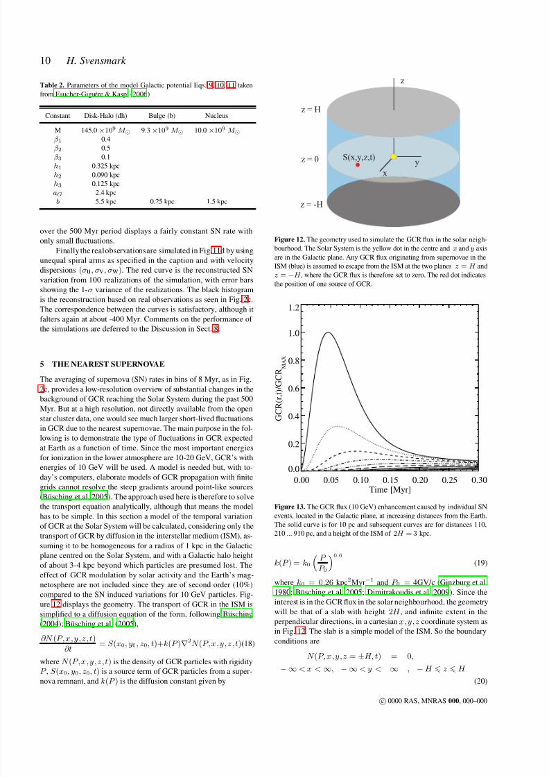
Table 2. Parameters of the model Galactic potential Eqs. 9, 10, 11 taken
from Faucher-Giguere & Kaspi (2006)
Constant Disk-Halo (dh) Bulge (b) Nucleus
M 145.0×10⁹ M ⊙ 9.3×10⁹ M ⊙ 10.0 ×10⁹ M ⊙β1 0.4
β2 0.5
β3 0.1
h1 0.325 kpc
h2 0.090 kpc
h3 0.125 kpc
aG 2.4 kpc
b 5.5 kpc 0.25 kpc 1.5 kpc
over the 500 Myr period displays a fairly constant SN rate with
only small fluctuations.
Finally the real observations are simulated in Fig.11d by using
unequal spiral arms as specified in the caption and with velocity
dispersions (σu, σv, σw). The red curve is the reconstructed SNvariation from 100 realizations of the simulation, with error bars
showing the 1-σ variance of the realizations. The black histogram
is the reconstruction based on real observations as seen in Fig. 2c.
The correspondence between the curves is satisfactory, although it
falters again at about -400 Myr. Comments on the performance of
the simulations are deferred to the Discussion in Sect. 8.
5 THE NEAREST SUPERNOVAE
The averaging of supernova (SN) rates in bins of 8 Myr, as in Fig.
2c, provides a low-resolution overview of substantial changes in the
background of GCR reaching the Solar System during the past 500
Myr. But at a high resolution, not directly available from the openstar cluster data, one would see much larger short-lived fluctuations
in GCR due to the nearest supernovae. The main purpose in the fol-
lowing is to demonstrate the type of fluctuations in GCR expected
at Earth as a function of time. Since the most important energies
for ionization in the lower atmosphere are 10-20 GeV, GCR’s with
energies of 10 GeV will be used. A model is needed but, with to-
day’s computers, elaborate models of GCR propagation with finite
grids cannot resolve the steep gradients around point-like sources
(Busching et al. 2005). The approach used here is therefore to solve
the transport equation analytically, although that means the model
has to be simple. In this section a model of the temporal variation
of GCR at the Solar System will be calculated, considering only the
transport of GCR by diffusion in the interstellar medium (ISM), as-
suming it to be homogeneous for a radius of 1 kpc in the Galacticplane centred on the Solar System, and with a Galactic halo height
of about 3-4 kpc beyond which particles are presumed lost. The
effect of GCR modulation by solar activity and the Earth’s mag-
netosphere are not included since they are of second order (10%)
compared to the SN induced variations for 10 GeV particles. Fig-
ure 12 displays the geometry. The transport of GCR in the ISM is
simplified to a diffusion equation of the form, following Busching
(2004); Busching et al. (2005),
∂N (P,x,y,z,t)
∂t= S (x0, y0, z 0, t)+k(P )∇2N (P,x,y,z,t)(18)
where N (P,x,y,z,t) is the density of GCR particles with rigidity
P , S (x0, y0, z 0, t) is a source term of GCR particles from a super-
nova remnant, and k(P ) is the diffusion constant given by
z = 0
z = H
z = -H
y
x
z
S(x,y,z,t)
Figure 12. The geometry used to simulate the GCR flux in the solar neigh-
bourhood. The Solar System is the yellow dot in the centre and x and y axis
are in the Galactic plane. Any GCR flux originating from supernovae in the
ISM (blue) is assumed to escape from the ISM at the two planes z = H and
z = −H , where the GCR flux is therefore set to zero. The red dot indicates
the position of one source of GCR.
0.00 0.05 0.10 0.15 0.20 0.25 0.30Time [Myr]
0.0
0.2
0.4
0.6
0.8
1.0
1.2
G C R ( r , t ) / G
C R
M A X
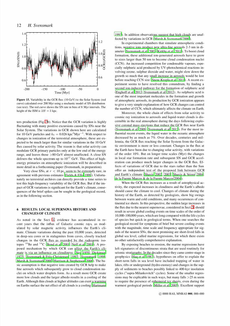
Figure 13. The GCR flux (10 GeV) enhancement caused by individual SN
events, located in the Galactic plane, at increasing distances from the Earth.
The solid curve is for 10 pc and subsequent curves are for distances 110,
210 ... 910 pc, and a height of the ISM of 2H = 3 kpc.
k(P ) = k0
P
P 0
0.6(19)
where k0 = 0.26 kpc2Myr−1 and P 0 = 4GV/c (Ginzburg et al.
1980; Busching et al. 2005; Dimitrakoudis et al. 2009). Since the
interest is in the GCR flux in the solar neighbourhood, the geometry
will be that of a slab with height 2H , and infinite extent in the
perpendicular directions, in a cartesian x,y,z coordinate system as
in Fig. 12. The slab is a simple model of the ISM. So the boundary
conditions are
N (P,x,y,z = ±H, t) = 0,
−∞ < x < ∞, −∞ < y < ∞ , −H z H
(20)
c 0000 RAS, MNRAS 000, 000–000

7/28/2019 Henryk SVENSMARK: Evidence of nearby supernovae affecting life on Earth (arXiv. org)
http://slidepdf.com/reader/full/henryk-svensmark-evidence-of-nearby-supernovae-affecting-life-on-earth-arxiv 11/21
Evidence of nearby supernovae affecting life on Earth 11
-1.0 -0.5 0.0 0.5 1.0x [kpc]
-1.0
-0.5
0.0
0.5
1.0
y [ k p c ]
a)
-1.0 -0.5 0.0 0.5 1.0x [kpc]
-0.3-0.2-0.1-0.00.10.20.3
z [ k p c ] b)
0 10 20 30 40 50
0.01
0.10
1.00
R [ k p
c ]
c)
0 10 20 30 40 50
Time [Myr]
0.00.2
0.4
0.6
0.8
1.01.2
F ( t ) / F
m a x
d)
Figure 14. Model of the frequency of supernovae resulting from a period
of ∆t = 8 Myr of initial star formation. a) is a uniform distribution of SNs
in the Galactic plane (x,y) for distances r < 1kpc. b) is the distribution
of SNs perpendicular to the Galactic plane with a scale height of 90 pc
(Miller & Scalo 1979). The height of the ISM is 2H = 3 kpc. c) is the tem-
poral distribution of SNs on a scale of 50 Myr, derived from the SNresponse
function, as a function of the distance from the Solar System. Finally d) is
the variation in GCR (10 GeV) caused by star formation in the initial ∆t
= 8 Myr interval. The tallest spikes in d) correspond with the nearest SNs
in c). The GCR curve is scaled to the present SN rate = 27 kpc−2Myr−1
(Grenier 2000).
The source function of GCR from one SN occurring at
(xi, yi, z i, ti) (Busching et al. 2005), is written as
S (P,x,y,z,t,xi, yi, z i, ti) =
(t− ti)exp−
t− tiτ
P
P 0
−αΘ(t− ti)×
δ (x− xi)δ (y− yi)δ (z − z i) (21)
where Θ(t) is the unit step function, and δ is the delta function, and
α is the slope of the source spectrum. The Green’s function for the
diffusion equation for a slab geometry is found from
∂G(x,y,z,x′, y′, z ′, t , t′)
∂t− k∇2G(x,y,z,x′, y′, z ′, t , t′) =
δ (x− x′
)δ (y− y′
)δ (z − z ′
)δ (t− t′
) (22)
and is
G(x,y,z,x′, y′, z ′, t , t′) =
1
4πkH (t− t′)exp
−
(x− x′)2 + (y− y′)2
4k(t− t′)
×
∞n=1
exp− πn2H
2 k(t− t′)×sin
πn(z + H )
2H
sin
πn(z ′ + H )
2H
(23)
The solution to the original equation becomes
N (x,y,z,t) = ∞
−∞
∞
−∞
H −H
tt′
G(x,y,z,x′, y′, z ′, t , t′)×
S (x′, y′, z ′, t′)dx′dy′dz ′dt′ (24)
Figure 13 shows an example for the above solution where the
enhancement of the GCR flux (10 GeV) caused by an individualSN, located in the Galactic plane, at increasing distances from the
Earth. It is then possible to simulate the effect of a large number
of SNs occurring at different times by simple superposition of the
solutions in Eq. 24. Assuming that the density of SNs varies in
accordance with the observed changes in the SN rates as calculated
from the open clusters, as in Fig. 2c, one can simulate a varying
GCR flux. The procedure is as follows:
• Use the calculated cluster production rate during the last 500
Myr (as shown in Fig. 2b), as the basis of the stochastic calculation.
• Estimate the number of massive stars that go supernova in a
time step of ∆t = 8 Myr by scaling SN(0) to the present rate of SN
in the 1 kpc region, as SN(0) = 27 kpc−2Myr−1 π 1 kpc2 8 Myr =
679 SN (Grenier 2000).
• Distribute the SN in space by using a random generator to
make a uniform distribution (x,y) in the Galactic plane in the 1 kpc
region, and an exponential distribution with a scale height of 90 pc
(Miller & Scalo 1979) around the alactic plane with coordinate z .Figs. 14a and 14b show one realization of such a spatial distribution
based on an 8 Myr time step.
• Having the estimated number of massive stars (the SN progen-
itors) in a time step ∆t, use the response function shown in Fig. 3 to
calculate a temporal probability distribution prescribing the times
ti when the massive stars go SN. Figure 14c shows the temporal
distribution and the distances of the SNs from the Solar System in
the following≈ 40 Myr.
• From the temporal and spatial distribution of SNs, calculate
the solution in Eq. 24 for each SN at distance and time (ri, ti),
and add the solutions to obtain the temporal GCR flux at the Solar
System.
Figure 14d shows the temporal evolution based on the above proce-
dure from a single time step ∆t = 8 Myr. The massive SN progen-
itors stars go SN with the coordinates (xi, yi, z i, ti) within a 1 kpc
distance in the solar neighbourhood and within an approximately
40 Myr period following the initial formation of the massive stars.
For each SN with a distance and a time the solution based on Eqn.
24 is calculated, and then all the solutions are added to give the
temporal variation at the position of the Solar System. As seen in
Fig. 14c and d only a relatively close SN results in a clear spike in
the GCR flux. Figure 15 illustrates one (random) realization of a
calculation of the GCR flux caused by the varying SN rate during
the past 200 Myr as determined from the estimate of open clus-
c 0000 RAS, MNRAS 000, 000–000
7/28/2019 Henryk SVENSMARK: Evidence of nearby supernovae affecting life on Earth (arXiv. org)
http://slidepdf.com/reader/full/henryk-svensmark-evidence-of-nearby-supernovae-affecting-life-on-earth-arxiv 12/21
12 H. Svensmark
-200 -150 -100 -50 0Time [Myr]
0.6
0.8
1.0
1.2
1.4
S N ( t ) / S N
( 0 )
0.6
0.8
1.0
1.2
G C R ( t ) / G C
R ( 0 )
Figure 15. Variability in the GCR flux (10 GeV) to the Solar System (red
curve) calculated over 200 Myr using a stochastic model of SN distribution
(see text). The red curve shows the SN rate in bins of 8 Myr intervals. The
height of the ISM is 2H = 3 kpc.
ters production (Fig. 2b). Notice that the GCR variation is highly
fluctuating with many positive excursions caused by SNs near the
Solar System. The variations in GCR shown here are calculated
for 10 GeV particles and k0 = 0.026 kpc2Myr−1. With respect to
changes in ionization of the terrestrial atmosphere, these are ex-
pected to be much larger than for similar variations in the 10 GeV
flux caused by solar activity. The reason is that solar activity can
modulate GCR primary particles only at the low end of the energy
range, and leaves those >80 GeV almost unaffected. A close SN
delivers the whole spectrum up to 1017 GeV. This effect of high-
energy primaries on atmospheric ionization will be described in
more detail in a forthcoming paper (Svensmark, in preparation).
Very close SNs, at r < 10 pc, seem to be extremely rare, inagreement with previous estimates (Fields & Ellis 1999). Unfortu-
nately no terrestrial archives can directly provide a time series to
test this high-frequency variability of the GCR flux. But if the im-
pact of GCR variations is significant for the Earth’s climate, conse-
quences of the brief spikes can be sought in the geological record,
as in the following section.
6 RESULTS: LOCAL SUPERNOVA HISTORY AND
CHANGES OF CLIMATE
As noted in the Sect. 1, evidence has accumulated in re-
cent years that the influx of Galactic cosmic rays, as mod-
ulated by solar magnetic activity, influences the Earth’s cli-mate. Climate variations during the past 10,000 years, detected
in deep-sea cores or in stalagmites from caves, closely tracked
changes in the GCR flux as recorded by the radiogenic iso-
topes 10Be and 14C (Bond et al. 2001; Neff et al. 2001). A pro-
posed mechanism by which GCR can affect the Earth’s cli-
mate is via an influence on cloudiness (Ney 1959; Dickinson
1975; Svensmark & Friis-Christensen 1997; Svensmark 1998;
Marsh & Svensmark 2000; Harrison & Stephenson 2006). The ba-
sic assumption is that negative ions created by GCR help to make
fine aerosols which subsequently grow to cloud condensation nu-
clei on which water droplets form. As a result more GCR create
more low clouds and the larger albedo results in a cooling of the
Earth. Although thin clouds at higher altitudes can exert a warming
on Earths surface the net effect of all clouds is a cooling (Hartmann
1993). In addition observations suggest that high clouds are unaf-
fected by variations in GCR (Marsh & Svensmark 2000).
In experimental chambers that simulate atmospheric condi-
tions, negative ions produce new ultra-fine aerosols 2-3 nm in di-
ameter (Svensmark et al. 2007; Kirkby et al. 2011). To boost cloud
formation, these additional ion-generated aerosols have to growto sizes larger than 50 nm to become cloud condensation nuclei
(CCN). An increased competition for condensable vapours, espe-
cially sulphuric acid produced by UV-photochemical reactions in-
volving ozone, sulphur dioxide and water, might slow down the
growth so much that any small increase in aerosols would be lost
before reaching CCN size (Snow-Kropla et al. 2011). A recent ex-
periment seems to have resolved this conundrum, by finding a
second ion-induced pathway for the formation of sulphuric acid
(Enghoff et al. 2012; Svensmark et al. 2012). As sulphuric acid is
one of the most important molecules in the formation and growth
of atmospheric aerosols, its production by GCR ionization appears
to give a very simple explanation of how GCR changes can control
the number of CCN, which ultimately affects the climate on Earth.
Moreover, the whole chain of effects from solar activity tocosmic ray ionization to aerosols and liquid-water clouds is dis-
cernible in the real atmosphere during the days following explo-
sive coronal mass ejections that reduce the GCR flux near Earth
(Svensmark et al. 2009; Svensmark et al. 2012). For the most in-
fluential recent events, the liquid water in the oceanic atmosphere
decreased by as much as 7%. Over decades, centuries and mil-
lennia, the GCR flux reaching the Solar System from the Galac-
tic environment is more or less constant. Changes in the flux at
the Earth have been due to changing solar activity, with variations
of the order 10%. But on longer time scales (Myr) the changes
in local star formation rate and subsequent SN and GCR accel-
eration can produce much larger changes in the GCR flux. Ef-
fects of variations of GCR due to the stars rather than the Sun
offer an independent test of the proposed link between GCRand Earth’s climate (Shaviv 2002, 2003; Shaviv & Veizer 2004;
de la Fuente Marcos & de la Fuente Marcos 2004).
When the GCR flux increases as a result of astrophysical ac-
tivity, the expected increases in cloudiness and the Earth’s albedo
should cause the climate to cool. Changes of climate during the
history of the Earth, as detected by geologists, show big swings
between warm and cold conditions, and many occurrences of con-
tinental ice sheets. In this perspective, the sudden large increases in
the flux due to the nearest supernovae, considered in Sect. 5, should
result in severe global cooling events on time scales of the order of
10,000-100,000 years, which are long compared with the life cycles
of species but quick in geological terms. When one searches the
geological record for symptoms of brief but severe cooling events
with the magnitude, time scale and frequency appropriate for sig-nals of the nearest SNs, the most promising are short-lived falls in
global sea level, called marine regressions, for which there exists
no other satisfactorily comprehensive explanation.
By exposing beaches to erosion, the marine regressions have
left signatures of discontinuous strata that are used routinely for
seismic stratigraphy. In the decades since they came centre-stage in
geophysics (Haq et al. 1987), hypotheses on offer to explain the
short-term falls in sea level have included trapping of water in
lakes, rifts or underground (hydro-eustasy) and changes in the sup-
ply of sediments to beaches possibly linked to 400-kyr insolation
cycles (”supra-Milankovitch” cycles). Some of the smaller regres-
sions may be explicable in such ways, but many falls >25 m seem
to require the presence of ephemeral ice sheets, even during the
warmest geological periods (Miller et al. 2005). Excellent support
c 0000 RAS, MNRAS 000, 000–000

7/28/2019 Henryk SVENSMARK: Evidence of nearby supernovae affecting life on Earth (arXiv. org)
http://slidepdf.com/reader/full/henryk-svensmark-evidence-of-nearby-supernovae-affecting-life-on-earth-arxiv 13/21
Evidence of nearby supernovae affecting life on Earth 13
-50 -40 -30 -20 -10 0Time [Myr]
0.2
0.4
0.6
0.8
1.0
1.2
S N ( t ) / S N ( 0 )
200
100
0
-100
S e a l e
v e l [ m ]
-50 -40 -30 -20 -10 0Time [Myr]
0.2
0.4
0.6
0.8
1.0
1.2
1.4
G C R ( t ) / G C R ( 0 )
Figure 16. (a) Short-lived falls in sea level (marine regressions) seen in the
stratigraphic record (data of Haq et al. (1987) obtained from Miller et al.
(2005)) during the past 50 Myr are suggested to be signals of the near-
est supernovae, enhancing GCR and provoking increased cloudiness and
glaciation. The blue curve in the top panel, where the right-hand scale is
inverted, shows an overall fall in global sea level due mainly to the loss
of ocean water into ice sheets of increasing volume grounded in the polarregions. The trend corresponds broadly to the overall SN rate (red curve),
here presented in bins of 3.5 Myr. Because of the scale inversion, the short-
lived marine regressions appear as brief spikes superimposed on the general
trend in sea level. In variance and frequency they resemble the excursions
in GCR modelled in Fig. 15, due to the nearest supernovae. In the lower
panel the simulated GCR flux (10 GeV) over the past 50 Myr incorporates
excursions due to the nearest individual supernovae. Note that this is just
one random realization of the statistics of SN events.
for the regressions history and a link to glaciations comes from
Billups & Schrag (2002) who used Mg/Ca and oxygen isotopes in
benthic foraminifera to assess changes over the past 27 Myr.
In the absence of other evidence for when the nearest SN
events occurred, the hypothesis that they provoked major marineregressions can be considered by referring to the fluctuations in
GCR calculated in Sec 5. Fig. 16 focuses on the sea level changes
over the past 50 Myr, shown in the top panel (scale inverted). Also
in the top panel is the varying SN rate (red curve), shown in this
case with a resolution of 3.5 Myr. The overall covariation of sea
levels and SN rates is good, but it becomes better in detail when an
arbitrary randomization of the SN events within each period of 3.5
Myr generates the GCR flux shown in the lower panel. The count
of major marine regressions includes ≈ 25 regressions of >25 m,
which can be compared with an expectation of ≈ 25 major GCR ex-
cursions due to the nearest supernova, as shown in the lower panel
of Fig. 16 (≈ 0.5 Myr−1). The aim here is not to try to achieve a
perfect covariance by further statistical iterations, but to illustrate
that, in the absence of any other explanation for them, the fast sea
-500 -400 -300 -200 -100 0Time [Myr]
0.4
0.6
0.8
1.0
1.2
1.4
S N ( t ) / S N ( 0 )
O S D C P Tr J K Pg Ng C m
Figure 17. Variations in SN rates during the past 500 Myr (red curve) to-
gether with a ±1-σ uncertainty (dark grey band) and ±1-σ uncertainty in-cluding Poisson noise (light grey band). The vertical dashed lines are the
separation between geological periods. The coloured band indicates cli-
matic periods as given in Table 3: warm periods (red), cold periods (blue),
glacial periods (white and blue hatched bars), and finally peak glaciations
(black and white hatched bars). Notice the correspondence between high
SN activity and cold/glacial climate. Abbreviations for geological periods
are: Cm, Cambrian; O, Ordovician; S, Silurian; D, Devonian; C, Carbonif-
erous; P, Permian; Tr, Triassic; J, Jurassic; K, Cretaceous; Pg, Palaeogene;
Ng, Neogene. Plot starts at -510 Myr.
level falls are just what are to be expected as signals of closer-than-
usual SN detonations.
The more persistent changes in sea level seen in Fig. 16 tell
a grander story about the build-up of ice sheets on Antarctica, asthe Earth began to develop its present glacial climate. It was a hesi-
tant process (Zachos et al. 2001) with major cooling and glaciation
beginning 33 Myr ago, a warmer interval starting 26 Myr ago, and
refreezing in the gradual build-up to recent ice volumes beginning
10-14 Myr ago. It can be seen from the red curve in the upper panel
that this timetable is broadly consistent with ups and downs in the
SN rate.
Reverting to the overall pattern of SN rates derived in Sect.
3, these can be compared with more gradual but larger changes
in climate in the past 500 Myr, alternating between persistently
warm and persistently cold conditions. Cold and glacial intervals
are listed in Table 3 and shown in the coloured band in Fig. 17. All
geological periods and dates are given with reference to the Ge-
ological Time Scale 2004 of Gradstein et al. (2005). Starting withdata from Royer (2006) and Saltzman (2005), a scan of the liter-
ature adds important details. Also noted are what seem to be the
”peak ice” times over long intervals, which are of interest for the
GCR hypothesis, although one should be aware that the magnitudes
of those glaciations differed greatly.
Despite the uncertainties about peering so far back in time,
both astrophysically and geologically, the association between cold
conditions and high SN rates stands out clearly in Fig. 17 and pro-
vides strong support for a very long-term GCR-climate link that is
independent of solar variations. Also noticeable in Fig. 17 is the
way most geological periods fit neatly around either an upturn or a
downturn the SN rates, suggesting that the transition from one pe-
riod to the next is connected to a major change in the astrophysical
environment.
c 0000 RAS, MNRAS 000, 000–000

7/28/2019 Henryk SVENSMARK: Evidence of nearby supernovae affecting life on Earth (arXiv. org)
http://slidepdf.com/reader/full/henryk-svensmark-evidence-of-nearby-supernovae-affecting-life-on-earth-arxiv 14/21
14 H. Svensmark
-200 -150 -100 -50 0
Time [Myr]
0.4
0.6
0.8
1.0
1.2
1.4
S N ( t ) / S N ( 0 )
-4
-2
0
2
4
δ 1 8 O [ p e r m i l l ]
J K Pg Ng
Figure 18. Measurements of δ18O over the last 200 Myr (coloured points)
compared with SN history over the same period (red curve). Light blue data
points are from Zachos et al. (2001) and grey circles are from Prokoph et al.
(2008). The dark blue curve is an average of the grey points. The light blue
points have been offset by -2.5 per mil relative to the grey data to take
account of the provenance of the data from deeper water.
Widely used as a quantitative measure of changes in tempera-
ture is the ratio between the two stable isotopes of oxygen, 18O and16O, found in sediments and fossil sea shells. Oceanic enrichment
with 18O occurs in cold conditions for physical reasons, of which
the simplest is that light water molecules with pure 16O evaporate a
little more readily. δ 18O is measured in parts per mill (i.e. parts perthousand) compared with a reference material (Vienna PDB, -2.2
per mill) and it is important to be aware of the provenance of the
data, because regional differences can obscure the global picture.
That is why, in comparing δ 18O with SN rates over the past 200
million years, in Fig. 18, prominence is given to results from care-
fully chosen mid-latitude sea shells (Zachos et al. 2001), although
other sources are also included (Prokoph et al. 2008). As one can
see in Fig. 18 there seems to be, with some exceptions, an overall
correspondence between δ 18O and SN rates.
7 RESULTS: ECOLOGICAL CORRELATIONS WITH
SUPERNOVA HISTORY
One index of success or setback for life in general is biodiversity.
The evolution of living creatures can be gauged by the rate of orig-
ination of new forms (classified, for example, as orders, families,
genera or species) and the rate of extinction of old forms. The dif-
ference at any stage results in an increase or decrease of global bio-
diversity. By counting known fossils, palaeontologists have found
large variations in marine biodiversity over the past 500 Myr. The
top panel of Fig. 19 shows the recently re-assessed genus-level di-
versity of marine invertebrate animals. One of the many intrinsic
and environmental factors suspected of influencing biodiversity is
sea level, shown in the lower panel of Fig. 19. Excluding the brief
marine regressions discussed earlier, this curve is the first-order en-
velope of long-term sea level. Conventionally, in plate tectonics, the
accretion of mid-ocean ridges during sea-floor spreading pushes up
-500 -400 -300 -200 -100 0
200
300
400500
600
700
800
N ( t ) [ G
e n e r a ]
-500 -400 -300 -200 -100 0t [Myr]
-200
-100
0
100
200
300
400
500
S e
a l e v e l [ m ]
0.5
1.0
1.5
2.0
2.5
3.0
Λ
( s e a l e v e l )
Figure 19. Upper panel: genus-level diversity of extant and extinct marine
invertebrates as an index of variable biodiversity (Alroy et al. (2008), based
on a sampling-standardized analysis of the Paleobiology Database). Lower
panel: First-order sea level variations attributable to tectonics (adapted from
Haq et al. (1987); Haq & Schutter (2008)).
-400 -300 -200 -100 0Time [Myr]
0.4
0.6
0.8
1.0
1.2
1.4
1.6
Γ ( t )
200
400
600
800
N ( t ) / Λ ( t )
S D C P Tr J K Pg Ng
Figure 20. SN history and marine invertebrate genera. The black curve is
based on the SN rates and given by Eq. 27. The blue curve shows marine
genera normalized with the sea level (Eq. 29) and defined as the right-hand
side of Eq. 28. The grey area is the 1-σ variance calculated from a Monte
Carlo simulation. The error bars on the genera (blue curve) show a min-
imum 1-σ uncertainty since an error estimate is not available for the sea
level data. Evidently marine biodiversity is largely explained by a combina-
tion of sea level and astrophysical activity.
c 0000 RAS, MNRAS 000, 000–000

7/28/2019 Henryk SVENSMARK: Evidence of nearby supernovae affecting life on Earth (arXiv. org)
http://slidepdf.com/reader/full/henryk-svensmark-evidence-of-nearby-supernovae-affecting-life-on-earth-arxiv 15/21
Evidence of nearby supernovae affecting life on Earth 15
Table 3. Episodes of glaciation and cold intervals as displayed in Fig. 17. (1) Saltzman (2005); (2) Saltzman & Young (2005); (3) Trotter et al. (2008); (4)
Royer (2006); (5) Fielding et al. (2008); (6) McArthur et al. (2007); (7) Bornemann et al. (2008); (8) Baumann & Huber (1999)
Period Myr BP Cold intervals Conditions Reference
Cm Cambrian 542 502 -492 Cold 1
O Ordovician 488.3 455.0 -443.7 Glacial 2
450 -445 Cold 1
445 -442 Peak ice 3
S Silurian 443.7 442 -415 Cold 1
D Devonian 416 375 -361.4 Cold 1
361.4 -360.6 Glacial 4
360.6 -359.2 Cold 1
C Carboniferous 359.2 375 -353 Cold 1
353 -349 Glacial 4
349 -345 Cold 1
326.5 -325.5 Glacial 5
322.5 -319.5 Glacial 5
317.0 -315.0 Glacial 5
P Permian 299 299 -294 Glacial 5
294 -291 Peak ice 5
287 -280 Glacial 5273 -268 Glacial 5
267 -260 Glacial 5
260 -251 Cold 4
Tr Triassic 251
J Jurassic 199.6 184 -183 Cold 4
167.7 -164.7 Cold 4
162 -159 Cold 4
150 -144 Cold 4
K Cretaceous 145.5 140.5 -139.5 Cold 4
137.5 -137 Cold 4
137 -136 Peak ice 6
125.0 -112.0 Cold 4
97.5 -96.5 Cold 4
91.3 -91.1 Glacial 7
91.1 -89 Cold 471.6 -69.6 Cold 4
67.5 -66.5 Cold 4
Pg Palaeogene 65.5 65.6 -65 Cold 4
33 -23.03 Glacial 4
Ng Neogene 23.03 23.03 -2.8 Glacial 4
2.8 -0 Peak ice 8
the sea level (Russell 1968). The long-term sea level minimum 200
Myr ago coincided with the completion of the supercontinent of
Pangaea, whilst the peaks in sea level 100-70 Myr and 450 Myr
ago were associated with the spreading of new oceans following
the breakup of Pangaea and of its predecessor Pannotia.
A higher sea level will result in flooding of low inland ar-
eas, and increase the total length of coastline and the area of the
continental shelves. This results in more heterogeneous habitats in
which species can evolve, leading to an increase in diversity, and
Miller et al. (2005) offer this as the reason for the development of
the three eukaryotic phytoplankton clades (lineages) that dominate
the modern ocean. But the rough correspondence between marine
invertebrate diversity and sea level seen in Fig. 19 is plainly not
the whole story. Here the novel assumption is that variations in SN
rates will also change conditions for the evolution of life by chang-
ing the climate and thereby altering, for example, the circulation
of nutrients and the variety of habitats between the Equator and
the poles. If the sea level and the changes in climate caused by SN
are both important one would expect that the temporal evolution of
marine invertebrate diversity N(t) should be a function of SN rate
Γ(SN, t) and sea level Λ(Sea¯level,t) written as
N(t) = Γ(SN, t)Λ(Sea¯level,t) + ǫ(t) (25)
where ǫ(t) is a hopefully small noise term. If the genera count is
normalized by the sea level, a possible effect of the astrophysics
will be as
Γ(SN, t) =N(t)
Λ(Sea¯level, t)
+ ǫ(t) (26)
where ǫ(t) again is a noise term. Finally, since a mass extinction
can require 10 - 40 Myr recovery time (Alroy 2008), it is further to
be expected that a large change in SN can also lead to a persistent
effect on the genera count. The function Γ(SN, t) should therefore
also depend on earlier times and the simplest relation is
Γ(SN, t) = ν 1 t
−∞
SN (t′)exp −λ(t− t′)dt′ + ν 2 (27)
c 0000 RAS, MNRAS 000, 000–000

7/28/2019 Henryk SVENSMARK: Evidence of nearby supernovae affecting life on Earth (arXiv. org)
http://slidepdf.com/reader/full/henryk-svensmark-evidence-of-nearby-supernovae-affecting-life-on-earth-arxiv 16/21
16 H. Svensmark
where ν 1 and ν 2 are constants. Inserting Eq. 27 in Eq. 26 one gets
N(t)
Λ(Sea¯level,t)
=
ν 1 t
−∞
SN (t′)exp −λ(t− t′)dt′ + ν 2 + ǫ(t) (28)
Notice that the left hand side depends only on terrestrial quantities
and the right hand side depends only on astrophysical quantities.
Finally the sea level function is approximated by the two first terms
of a Taylor expansion of Λ(Sea¯level,t) as
Λ(Sea¯level,t) = α + β Sea
¯level(t) (29)
where α and β are constants. Figure 20 shows, as the blue curve,
the left-hand side of Eq. 28 which is the ratio between N(t) and
Λ(Sea¯level,t). The black curve in Fig. 20 is the right-hand side
of Eq. (28). The curves are displayed for α = 1, β = 1/250 m−1
and λ = 1/20 Myr−1 . These values ensure the best agreement be-
tween the astrophysical part (right-hand side of Eq. (28)) and the
terrestrial part (the left-hand side of Eq. (28)). The correlation co-
efficient is 0.89 for the last 400 Myr. Notice the overall agreement
between the blue and black curve, which gives confidence in the
basic assumption made in Eq. 25, namely that the chief governors
of marine invertebrate diversity are tectonics (sea level) and astro-
physics (local SN rate).
Another global index of life’s successes and setbacks, to con-
sider alongside biodiversity, is its primary productivity. This is the
rate at which all the world’s carbon-fixing micro-organisms and
plants, powered typically by sunlight, assimilate carbon for their
own growth and for the eventual nourishment of animals and fungi.
As the motor of the carbon cycle, the production of organic ma-
terial removes carbon dioxide from oceanic water and the atmo-
sphere, and replaces it with oxygen. A simple working hypothesis,
suggested by carbon-isotope data for the past 4 Gyr (Svensmark 2006a), is that primary productivity increases in glacial conditions,
perhaps because of better nutrient supplies, caused by a more vig-
orous mixing in the oceans during cold conditions. This hypothesis
(to be discussed later) would predict:
(i) A drawdown of CO2 from the environment in glacial condi-
tions. Since organic productivity consumes CO2 there should be an
impact on the levels of atmospheric and oceanic CO2. High pro-
ductivity draws down CO2, until ultimately the productivity rise
is halted not only by exhaustion of nutrients but by the scarcity
of CO2, which should prevent a total loss of environmental CO2.
Conversely, low productivity should result in an accumulation of
underemployed CO2.
(ii) Due to the increased organic productivity an increase in the
heavy stable isotope of carbon, 13C, is expected in the oceans dur-
ing glacial conditions.
As glacial versus warm conditions seem to follow SN rates (Figs.
17 and 18) one can look for matches between CO2, 13C and SN
rates. In the case of CO2, data are sparse in the earlier part of the
500-Myr record considered here, but more abundant later. In Fig.
21 the proxies for CO2 are paleosols (fossil soils) which offer the
longest time-span although less accurate at low CO2 (Royer et al.
2001) and fossilplanktonic foraminifera organisms from the oceans
(Royer 2006). The CO2 scale is inverted because because high SN
rates (cold climate) and low CO2 go together, and the logarithm
of the CO2 concentrations is used, on the assumption that the rela-
tion is not linear, in particular when the when CO2 is scarce. The
match between CO2 and SN rates encourages further pursuit of the
-500 -400 -300 -200 -100 0Time [Myr]
0.2
0.4
0.6
0.8
1.0
1.2
1.4
S N ( t ) / S N ( 0 )
4.0
3.5
3.0
2.5
2.0
1.5
L o g
1 0
( C O
2 ) [ p p m ]
O S D C P Tr J K Pg Ng C m
Figure 21. Used here as a proxy for Galactic cosmic rays (GCR) reaching
the Earth, the local supernova rate (red curve) from Fig. 2c is compared
with the logarithm of concentrations of CO2 in the air (grey circles, scale
inverted). The filled circles show CO2 data from δ13C in palaeosols and the
open circles are from foraminifera (Royer 2006). The plot gives an overall
impression of CO2 diminishing in cold conditions associated with high SN
rates, possibly because of drawdown of CO2 by photosynthesis in better
fertilized oceans (see text). Logarithms are used because drawdown should
be self-limiting when little CO2 is available. Geological periods are shown
by their abbreviations as in Table 3.
hypothesis in respect of δ 13C, as a possible indicator of primary
productivity.
When organisms take in carbon to grow, mainly as CO2 in
photosynthesis, they prefer molecules without the rarer (1%) 13C,
and so become enriched in 12C . When they die and decay they usu-
ally return their enriched carbon to the environment, but not always.
In the oceans, some of the dead phytoplankton, and other organisms
that have fed on their 12C-enriched constituents, become incorpo-
rated into seabed deposits or trapped in deep water by a failure of
the oceanic circulation. On land, some plants become buriedas peat
or coal. Organic carbon sequestration and the loss of enriched 12C
leaves the global environment enriched in 13C. This becomes ap-
parent in samples of surviving sea-floor deposits of inorganic car-
bonate and in the fossils of organisms that lived in the 13C-enriched
environment. As the global mixing time for seawater is of the order
1000 years, the regional influences on δ 13C should tend to aver-
age out on the million-year scale considered here. The definition of
δ 13C is given by
δ 13C(per mill) =
13C 12C
Sample
− 113C 12C
Reference
× 1000 (30)
where measurements are referred to (13C/12C )reference =
0.0112372 (Vienna PDB). The carbon cycle is an interaction be-
tween different reservoirs, and its mass balance for the ocean (fol-
lowing Kump & Arthur (1999)) can be written as
dM 0dt
= F w’ − (F b,org + F b,carb) (31)
where, M 0 is the change in carbon mass in the ocean atmosphere
system, F w’ is the input of carbon from weathering and volcanoes,
c 0000 RAS, MNRAS 000, 000–000

7/28/2019 Henryk SVENSMARK: Evidence of nearby supernovae affecting life on Earth (arXiv. org)
http://slidepdf.com/reader/full/henryk-svensmark-evidence-of-nearby-supernovae-affecting-life-on-earth-arxiv 17/21
Evidence of nearby supernovae affecting life on Earth 17
-500 -400 -300 -200 -100 0Time [Myr]
0.0
0.5
1.0
1.5
S N ( t ) / S N ( 0 )
-2
0
2
4
6
8
δ 1 3 C
[ p e r m i l l ]
O S D C P Tr J K Pg Ng
Figure 22. Changes in the global carbon cycle over the past 500 Myr are
reflected in the proportions of carbon-13 in sediments (δ13C in parts per
mill) shown by the scattered points, and compared here with the varia-
tions in the local supernova (SN) rate (red curve). Circles are δ13C in
marine carbonates: Cambrian (not labelled) to Carboniferous C (Saltzman
2005), Permian P (Grossman et al. 2008), Permo-Triassic transition P-Tr
(Kakuwa & Matsumoto 2006), Triassic T (Korte et al. 2005), Jurassic Jto Cretaceous K (Emeis & Weissert 2009) and Cretaceous K (Jarvis et al.
2006). Star symbols are δ13C in fossil organic matter (offset by 27 per
mill): Jurassic J to Neogene Ng (Falkowski et al. 2005). The black dashed
line is a smoothing of the δ13C data. Notice that there are three brief gaps
in the δ13C data (End-Silurian, Mid-Carboniferous and Mid-Jurassic). The
plot starts at -510 Myr.
F b,org is the input from organic matter and finally F b,carb is the
carbon input from carbonate minerals. From this the change in the
oceanic (marine carbonate) carbon isotope reservoir becomes
dM 0δ carbdt
= F w’δ w’−F b,carbδ carb−F b,org(δ carb +∆B)(32)
where ∆B = δ org − δ carb is the isotopic difference between or-
ganic matter and carbonate deposited in the ocean (typically of the
order -25 per mil1). On the time scales of Myr the above equations
reduce to steady state (dM 0/dt = 0), and simple algebra gives
f org =F b,org
F w’ + F b,org=
δ w’ − δ carb∆B
(33)
which indicates, under the assumption that the terms δ w’ and ∆Bare constant, that the term δ carb is related to the fraction of car-
bon buried as organic matter. Fig. 22 shows the variations in 13C
recorded as δ carb (Cambrian to Cretaceous) and δ org (Jurassic to
Neogene) from sources cited in the caption. The red curve is the
variation in SN rate during the last 510 Myr. Despite the large vari-
ability in δ 13
C in each time interval, a dominant influence of the
SN rate plainly over-rides all the complex practical and theoretical
reasons why such coherence with δ 13C might not be expected (see
Sect. 8). Considered together with the climatic evidence in Figs.
17 and 18, the palaeobiological Figs. 20, 21, and 22 give a strong
impression of impacts of SN rates on both the evolution and pro-
ductivity of life over the past 500 Myr. The interpretation of these
empirical results is discussed below.
8 DISCUSSION
8.1 Galactic structure and supernova rates in the Earth’s
vicinity (Sections 2-5)
Given the uncertainties about the Milky Way, it seemed entirely
possible at the outset of the quest for local supernova rates over
500 million years that complexities of Galactic structure, disper-
sal of open clusters by orbital diffusion, or insufficient data would
frustrate the effort. In the outcome, the results are sufficiently co-
herent to give a convincing match to known spiral arms (Fig. 5). Atthe same time they are sufficiently variegated to shed new light on
Galactic structure, and in particular on big differences in structure
outside and inside the solar circle seen in Figs. 6 and 7.
For the primary reckoning of SN rates in the solar neighbour-
hood, seen in Fig. 2c, the size of the region around the Solar System
was chosen to be large enough for a sufficient number of clusters
in the statistical ensemble, and small enough for the ensemble to be
as complete as possible. As seen in Fig. 1 these requirements limit
the preferred radius to about 0.85 kpc. Although using a different
radius does change the shape of the resulting SN curves, in the
vicinity of 0.85 kpc the change is not large. The decay law for open
clusters, given in Eq. 2, is a simple law that fits the data. One could
argue that the decay of very young clusters is different from older
clusters, warranting a decay law with two exponents that could re-sult in a larger estimate of the number of old clusters, but the sim-
pler approach with only one exponent in Eq. 2 is preferred. Chang-
ing the exponent within the 1-σ range leads to a small shift in the
overall slope of the SN curve. Finally the parameters used in the
Starburst99 program to estimate the SN response curve seen in Fig.
3 can also be changed, which in some cases results in marginally
different response functions, and therefore changes in the resulting
SN curves. Again, these changes are not large.
Diffusion of clusters in and out of the small region occurs in
the course of time, and large initial velocity dispersions would cer-
tainly erase information about the oldest clusters forming in the so-
lar neighbourhood. Results of a searching examination of the effect
of velocity dispersions, using the model in Sect. 4, are not discour-
aging, and in any case they may be overstating the dispersions. Thesimulations assume that the clusters were formed independently
and an uncorrelated Gaussian distribution of velocities is used. This
view may be too simple. As shown by Piskunov, A. E. et al. (2006)
there seem to be cluster complexes consisting of 10-100 clusters
that have a common dynamical origin, presumably because they
were born in the same giant molecular cloud. Clusters that are
members of the resulting ”families” have similar ages and are lo-
cated at similar distances. In the simulations in Sec. 4 such dy-
namical correlations are not included. If they were included, the
likely result would be a smaller overall dispersion of the clusters,
with better retention of the cluster formation history in the solar
neighbourhood. The simulations shown in Sect. 4 may therefore be
worst-case scenarios.
They also make it unlikely that the ages of nearby clusters are
c 0000 RAS, MNRAS 000, 000–000
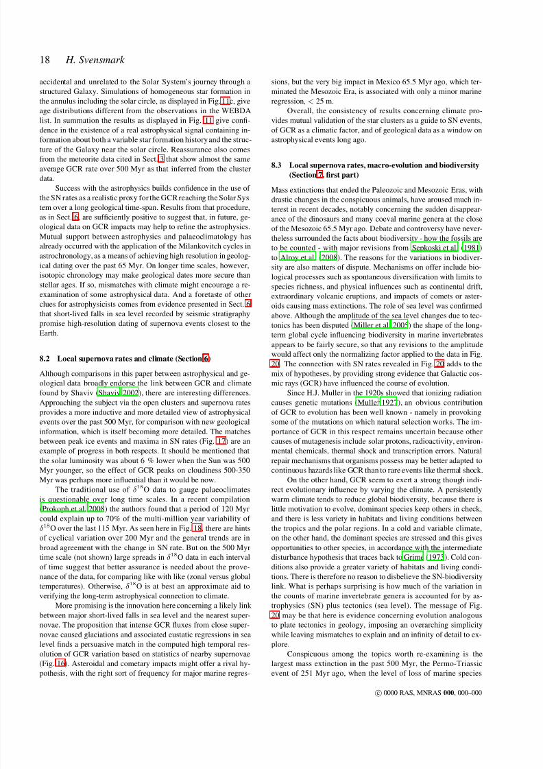
7/28/2019 Henryk SVENSMARK: Evidence of nearby supernovae affecting life on Earth (arXiv. org)
http://slidepdf.com/reader/full/henryk-svensmark-evidence-of-nearby-supernovae-affecting-life-on-earth-arxiv 18/21
18 H. Svensmark
accidental and unrelated to the Solar System’s journey through a
structured Galaxy. Simulations of homogeneous star formation in
the annulus including the solar circle, as displayed in Fig. 11c, give
age distributions different from the observations in the WEBDA
list. In summation the results as displayed in Fig. 11 give confi-
dence in the existence of a real astrophysical signal containing in-
formation about both a variable star formation history and the struc-
ture of the Galaxy near the solar circle. Reassurance also comes
from the meteorite data cited in Sect. 3 that show almost the same
average GCR rate over 500 Myr as that inferred from the cluster
data.
Success with the astrophysics builds confidence in the use of
the SN rates as a realistic proxy for the GCRreaching the Solar Sys-
tem over a long geological time-span. Results from that procedure,
as in Sect. 6, are sufficiently positive to suggest that, in future, ge-
ological data on GCR impacts may help to refine the astrophysics.
Mutual support between astrophysics and palaeoclimatology has
already occurred with the application of the Milankovitch cycles in
astrochronology, as a means of achieving high resolution in geolog-
ical dating over the past 65 Myr. On longer time scales, however,isotopic chronology may make geological dates more secure than
stellar ages. If so, mismatches with climate might encourage a re-
examination of some astrophysical data. And a foretaste of other
clues for astrophysicists comes from evidence presented in Sect. 6
that short-lived falls in sea level recorded by seismic stratigraphy
promise high-resolution dating of supernova events closest to the
Earth.
8.2 Local supernova rates and climate (Section 6)
Although comparisons in this paper between astrophysical and ge-
ological data broadly endorse the link between GCR and climate
found by Shaviv (Shaviv 2002), there are interesting differences.
Approaching the subject via the open clusters and supernova ratesprovides a more inductive and more detailed view of astrophysical
events over the past 500 Myr, for comparison with new geological
information, which is itself becoming more detailed. The matches
between peak ice events and maxima in SN rates (Fig. 17) are an
example of progress in both respects. It should be mentioned that
the solar luminosity was about 6 % lower when the Sun was 500
Myr younger, so the effect of GCR peaks on cloudiness 500-350
Myr was perhaps more influential than it would be now.
The traditional use of δ 18O data to gauge palaeoclimates
is questionable over long time scales. In a recent compilation
(Prokoph et al. 2008) the authors found that a period of 120 Myr
could explain up to 70% of the multi-million year variability of
δ 18O over the last 115 Myr. As seen here in Fig. 18, there are hints
of cyclical variation over 200 Myr and the general trends are inbroad agreement with the change in SN rate. But on the 500 Myr
time scale (not shown) large spreads in δ 18O data in each interval
of time suggest that better assurance is needed about the prove-
nance of the data, for comparing like with like (zonal versus global
temperatures). Otherwise, δ 18O is at best an approximate aid to
verifying the long-term astrophysical connection to climate.
More promising is the innovation here concerning a likely link
between major short-lived falls in sea level and the nearest super-
novae. The proposition that intense GCR fluxes from close super-
novae caused glaciations and associated eustatic regressions in sea
level finds a persuasive match in the computed high temporal res-
olution of GCR variation based on statistics of nearby supernovae
(Fig. 16). Asteroidal and cometary impacts might offer a rival hy-
pothesis, with the right sort of frequency for major marine regres-
sions, but the very big impact in Mexico 65.5 Myr ago, which ter-
minated the Mesozoic Era, is associated with only a minor marine
regression, < 25 m.
Overall, the consistency of results concerning climate pro-
vides mutual validation of the star clusters as a guide to SN events,
of GCR as a climatic factor, and of geological data as a window on
astrophysical events long ago.
8.3 Local supernova rates, macro-evolution and biodiversity
(Section 7, first part)
Mass extinctions that ended the Paleozoic and Mesozoic Eras, with
drastic changes in the conspicuous animals, have aroused much in-
terest in recent decades, notably concerning the sudden disappear-
ance of the dinosaurs and many coeval marine genera at the close
of the Mesozoic 65.5 Myr ago. Debate and controversy have never-
theless surrounded the facts about biodiversity - how the fossils are
to be counted - with major revisions from Sepkoski et al. (1981)
to Alroy et al. (2008). The reasons for the variations in biodiver-
sity are also matters of dispute. Mechanisms on offer include bio-logical processes such as spontaneous diversification with limits to
species richness, and physical influences such as continental drift,
extraordinary volcanic eruptions, and impacts of comets or aster-
oids causing mass extinctions. The role of sea level was confirmed
above. Although the amplitude of the sea level changes due to tec-
tonics has been disputed (Miller et al. 2005) the shape of the long-
term global cycle influencing biodiversity in marine invertebrates
appears to be fairly secure, so that any revisions to the amplitude
would affect only the normalizing factor applied to the data in Fig.
20. The connection with SN rates revealed in Fig. 20 adds to the
mix of hypotheses, by providing strong evidence that Galactic cos-
mic rays (GCR) have influenced the course of evolution.
Since H.J. Muller in the 1920s showed that ionizing radiation
causes genetic mutations (Muller 1927), an obvious contributionof GCR to evolution has been well known - namely in provoking
some of the mutations on which natural selection works. The im-
portance of GCR in this respect remains uncertain because other
causes of mutagenesis include solar protons, radioactivity, environ-
mental chemicals, thermal shock and transcription errors. Natural
repair mechanisms that organisms possess may be better adapted to
continuous hazards like GCR than to rare events like thermal shock.
On the other hand, GCR seem to exert a strong though indi-
rect evolutionary influence by varying the climate. A persistently
warm climate tends to reduce global biodiversity, because there is
little motivation to evolve, dominant species keep others in check,
and there is less variety in habitats and living conditions between
the tropics and the polar regions. In a cold and variable climate,
on the other hand, the dominant species are stressed and this givesopportunities to other species, in accordance with the intermediate
disturbance hypothesis that traces back to Grime (1973). Cold con-
ditions also provide a greater variety of habitats and living condi-
tions. There is therefore no reason to disbelieve the SN-biodiversity
link. What is perhaps surprising is how much of the variation in
the counts of marine invertebrate genera is accounted for by as-
trophysics (SN) plus tectonics (sea level). The message of Fig.
20 may be that here is evidence concerning evolution analogous
to plate tectonics in geology, imposing an overarching simplicity
while leaving mismatches to explain and an infinity of detail to ex-
plore.
Conspicuous among the topics worth re-examining is the
largest mass extinction in the past 500 Myr, the Permo-Triassic
event of 251 Myr ago, when the level of loss of marine species
c 0000 RAS, MNRAS 000, 000–000

7/28/2019 Henryk SVENSMARK: Evidence of nearby supernovae affecting life on Earth (arXiv. org)
http://slidepdf.com/reader/full/henryk-svensmark-evidence-of-nearby-supernovae-affecting-life-on-earth-arxiv 19/21
Evidence of nearby supernovae affecting life on Earth 19
reached 80-96% and two-thirds of tetrapod families went extinct
on land along with eight orders of insects (Sahney & Benton 2008).
The main hypotheses competing to explain it invoke volcanism in
Siberia or impacts by asteroids or comets, and part of the marine
loss can be attributed to an exceptionally low long-term sea level
(Fig. 19). But the Permo-Triassic event also coincided with the
largest decrease in SN rates from one 8 Myr bin to the next in
the whole 500 Myr period, as seen at -252 Myr in Fig. 17. That
was when Solar System had left the very active Norma spiral arm.
Fatal consequences would ensue for marine life if a rapid warm-
ing led to nutrient exhaustion (see below) occurring too quickly
for species to adapt. Before the culminating Permo-Triassic event,
the earlier Guadalupian-Lopingian mass extinction occurred about
265 Myr ago. By contrast, this was linked with global cooling that
interrupted a mid-Permian warming, and with a large increase in
δ 13C in the interval 265-260 Myr. Isozaki et al. (2007) point out
that prominent victims of this extinction were warm-water fauna
including gigantic bivalves and rugose corals. The full sequence of
warming, cooling and precipitate re-warming in the latter part of
the Permian period conforms very well with the variations in SNrates.
8.4 Local supernova rates: δ 13C and bio-productivity
(Section 7, second part)
The working hypothesis mentioned above, that in SN-induced
glacial conditions primary productivity increases and leads to draw-
down of CO2 and 12C sequestration, is compatible with the empir-
ical result in Fig. 22. A reality check comes from remarkable peaks
in reef carbonate production 430, 380, 290, 150 and 20 Myr ago
(Kiessling (2005), Supp. Fig. 3). All of these peaks coincide with
high SN rates, except for the maximum in the SN rate 150 Myr ago,
which was relatively weak. A link between SN rates and produc-
tivity is therefore clear, but in view of the complexity of the carboncycle and the many factors governing organic carbon burial or en-
trapment, and hence δ 13C, it might be unwise to conclude that the
mechanism is as simple as stated.
On the other hand, investigators have often noted the coinci-
dence of δ 13C excursions with climaticepisodes. For example, high
values of δ 13C in the Silurian Period are linked (Stricanne et al.
2006) to episodes of aridity in the tropics, which are often associ-
ated with polar glaciation, although that is questioned in this par-
ticular case. Over a longer timespan, Cambrian to Permian, large
increases in δ 13C were rare during hothouse climates but com-
mon during cool periods (Saltzman 2005). The productivity of the
oceans is limited by the supply of nitrogen in the near-surface wa-
ters, which is turn is limited by the availability of iron needed by
oceanic nitrogen-fixing cyanobacteria. During recent glacial peri-ods, iron delivered by windblown dust was at least an order of
magnitude higher than during interglacial periods (Falkowski et al.
1998) and at the Last Glacial Maximum ≈20 kyr ago organic car-
bon concentrations in the sediment of the eastern equatorial Pa-
cific were twice those of the past 11 kyr (Holocene) (Pichevin et al.
2009).
Occurrences of anoxia (regional exhaustion of oxygen) have
been offered as an explanation for the variability in δ 13C in cold
periods, with episodic organic carbon burial sustained by posi-
tive feedbacks between productivity and anoxia, whilst more sta-
ble δ 13C regimes in warm periods, which can last >10 Myr, may
tell of a nitrogen-limited ocean in which anoxia leads to increased
denitrification (Saltzman 2005). In addition, exhaustion of nutrients
can curb productivity in cold periods, causing variations in δ 13
C.
A related matter for consideration is the likely contribution to δ 13C
variations of the short-lived glacial episodes apparently linked to
the nearest supernovae (Sect. 6). For nearly all of the geological
record of the past 500 million years, long-term variations of δ 13C
from organic and carbonate sources have gone up and down more
or less in step. There is, however, a marked divergence in the most
recent part of the record that may be connected with the emergence
of C4 terrestrial plants, which have an extra carbon atom in their
first photosynthetic molecules and markedly higher δ 13C compared
with the commoner C3 plants (Osborne & Beerling 2006). In Fig.
22 there is a good match between organic δ 13C data to rising SN
rates in the past 20 Myr, but carbonate δ 13C (not shown) dimin-
ished.
These are only hints about how the empirical evidence about
δ 13C may be explained, and future theoretical inputs will no doubt
go far beyond the working hypothesis of drawdown and burial. The
challenge is similar to the case of biodiversity, for which many pro-
cesses of evolution and extinction exist and yet a dominant role
for astrophysics is discernible. In the same spirit, specialists are
invited to make of what they can of the δ
13
C link to the SN rateseen in Fig. 22. Finally, biological activity from phytoplankton is
a source of sulphur compounds in the atmosphere and therefore
also of cloud condensation nuclei (Charlson et al. 1987). So a sig-
nificant increase in biological productivity associated with a cool-
ing climate would give positive feedback on cloud formation and
thereby encourage further cooling. Conversely, nutrient limitation
due to either excessive productivity or weak circulation could exert
a warming effect by reducing cloud formation.
Other processes might in principle counter a cooling of the
climate by negative feedback. For example, if a cooling reduces
the loss of CO2 to geochemical weathering, that could lead to a
buildup of CO2 if other sinks and sources of CO2 remain constant,
and so dampen or reverse the cooling (Donnadieu et al. 2009). The
net impact of such processes will eventually have to be resolved byestimating the forcing of the individual processes and incorporating
them in a multidisciplinary numerical model beyond the scope of
this paper.
8.5 Caveats
The present results are no better than the data on which they are
built, and the uncertainty of the data gets larger as one reaches fur-
ther into the past. Estimated variations in SN rates are better deter-
mined for 250 - 0 Myr ago than for 500 - 250 Myr ago, because
there are fewer clusters of old ages and because phase mixing tends
to erase part of the memory of the birthplaces of the open clusters.
On the other hand, consistencies in the comparisons with geologi-
cal data lend support to the estimated SN rates, even in the earlier
period. Without direct terrestrial records of the GCR variation on
long time scales, the highly fluctuating flux due to nearby SNs re-
mains a matter of numerical modelling, but again the geological
record of sudden drops in sea level appears to support the analysis.
It remains to be seen whether future improvements in astrophysical
and geological data will show them continuing to mesh in the ways
suggested here.
9 CONCLUSION
The impact of stellar and interstellar processes on the Earth has
been addressed many times but, with the exception of Shaviv
c 0000 RAS, MNRAS 000, 000–000

7/28/2019 Henryk SVENSMARK: Evidence of nearby supernovae affecting life on Earth (arXiv. org)
http://slidepdf.com/reader/full/henryk-svensmark-evidence-of-nearby-supernovae-affecting-life-on-earth-arxiv 20/21
20 H. Svensmark
(2002), the speculations about episodic effects of e.g. a closer-
than-usual SN (Fields & Ellis 1999) or variations in the interstellar
medium (Frisch 2000) have demonstrated no persistent influence
on life and climate. The present paper has aimed at revealing the
integrated effect of varying GCR flux on the Earth during the past
500 Myr by reconstructing the SN rate during this period, and com-
paring it with geophysical and palaeobiological data.
Using the WEBDA database on open cluster formation, the
SN rate in the solar neighbourhood ( < 0.85 Kpc) was constructed,
and the variation was shown to be a superposition of two distinct
features originating either inside or outside the solar circle. Outside
the solar circle are four clear maxima in the SN reconstruction at
372.6, 269.1, 140.6, and 17.3 Myr before present, which are inter-
preted as the Solar System’s encounters with four spiral arms, lead-
ing to a relative angular frequency of the Solar System Ω0 − ΩP
= 13.0 ± 0.9 km s−1kpc−1 (or ΩP /Ω0 = 0.57± 0.5). Inside the
solar circle the pattern is not simple. In checking that the veloc-
ity dispersions of clusters do not erase the star formation history,
a model simulating cluster motions in and out of the solar neigh-
bourhood gave satisfactory results, even without taking account of the beneficial effect of the birth of many clusters in families with
relatively low dispersions.
In addition it was shown that multiple SN sources generate a
highly fluctuating GCR signal and that the nearest SNs (closer than
≈ 300 pc) produce clear spikes in the GCR flux. Those provided
the first link to the terrestrial climate noted here, with previously
unexplained short-lived falls in sea level accounted for by sudden
but brief glaciations caused by the nearest SNs, as in Fig. 16. The
match of longer-term climate to SN rates, seen in Figs. 17 and 18
leaves room only for relatively small or brief climatic influences
of all the tectonic, volcanic, and other processes discussed in this
connection. If the dominant role of the Galaxy in the terrestrial en-
vironment is further validated by ongoing studies, cosmic and ter-
restrial, it promises to simplify Phanerozoic climatology.As for the palaeobiology, remarkable connections to the long-
term histories of life and the carbon cycle have shown up unbidden
(Figs. 20, 21, 22). Biodiversity, CO2 and δ 13C all appear so highly
sensitive to supernovae in our Galactic neighbourhood that the bio-
sphere seems to contain a reflection of the sky.
ACKNOWLEDGMENTS
This research has made use of the WEBDA database
(http://www.univie.ac.at/webda/), operated at the Institute for
Astronomy of the University of Vienna. The author also thanks the
many geoscientists who have provided data and helpful comments,
and Nigel Calder for general discussions regarding this work.
REFERENCES
Alroy J., 2008, Proceedings of the National Academy of Science,
105, 11536
Alroy J., Aberhan M., Bottjer D. J., Foote M., Fursich F. T., Har-
ries P. J., Hendy A. J. W., Holland S. M., Ivany L. C., Kiessling
W. e. a., 2008, Science, 321, 97
Baumann K., Huber R. H., 1999, Proceedings of the Ocean
Drilling Program, Scientific Results. Edited by Raymo, M.E.,
Jansen, E., Blum, P., and Herbert, T.D., 162, 179
Berezhko E. G., Volk H. J., 2007, ApJl, 661, L175
Billups K., Schrag D. P., 2002, Paleoceanography, 17, 1003
Binney J., Tremaine S., 1987, Galactic dynamics. Princeton, NJ,
Princeton University Press, 1987, 747 p.
Blitz L., Fich M., Kulkarni S., 1983, Science, 220, 1233
Bond G.,Kromer B., Beer J., Muscheler R.,Evans M. N.,Showers
W., Hoffmann S., Lotti-Bond R., Hajdas I., Bonani G., 2001,
Science, 294, 2130
Bornemann A., Norris R. D., Friedrich O., Beckmann B.,
Schouten S., Damste J. S. S., Vogel J., Hofmann P., Wagner T.,
2008, Science, 319, 189
Boulares A., Cox D. P., 1990, ApJ, 365, 544
Busching I., 2004, PhD thesis, Fakultat fur Physik und As-
tronomie der Ruhr-Universitat Bochum
Busching I., Kopp A., Pohl M., Schlickeiser R., Perrot C., Grenier
I., 2005, ApJ, 619, 314
Chandar R., Fall S. M., Whitmore B. C., 2006, ApJ, 650, L111
Charlson R. J., Warren S. G.,LovelockJ. E., AndreaeM. O.,1987,
Nature, 326, 655
Dame T. M., Hartmann D., Thaddeus P., 2001, ApJ, 547, 792
de la Fuente Marcos R., de la Fuente Marcos C., 2004, New As-
tronomy, 10, 53de la Fuente Marcos R., de la Fuente Marcos C., 2008, ApJ, 672,
342
Dias W. S., Alessi B. S., Moitinho A., Lepine J. R. D., 2002, As-
tronomy and Astrophysics, 389, 871
Dias W. S., Alessi B. S., Moitinho A., Lepine J. R. D., 2010,
VizieR Online Data Catalog, 1, 2022
Dickinson R. E., 1975, Bull. American Meteorol. Soc., Vol. 56,
p. 1240 - 1248, 56, 1240
Dimitrakoudis S., Mastichiadis A., Geranios A., 2009, Astropar-
ticle Physics, 31, 13
Donnadieu Y., Godderis Y., Bouttes N., 2009, Climate of the Past,
5, 85
Emeis K., Weissert H., 2009, Sedimentology, 56, 247
Enghoff M. B., Bork N., Hattori S., Meusinger C., NakagawaM., Pedersen J. O. P., Danielache S., Ueno Y., Johnson M. S.,
Yoshida N., Svensmark H., 2012, Atmospheric Chemistry and
Physics Discussions, 12, 5039
Enghoff M. B., Pedersen J. O. P., Uggerhøj U. I., Paling S. M.,
Svensmark H., 2011, Geophysical Research Letters, 38, L09805
Falkowski P. G., Barber R. T., Smetacek V., 1998, Science, 281,
200
Falkowski P. G., Katz M. E., Milligan A. J., Fennel K., Cramer
B. S., Aubry M. P., Berner R. A., Novacek M. J., Zapol W. M.,
2005, Science, 309, 2202
Faucher-Giguere C., Kaspi V. M., 2006, ApJ, 643, 332
Fielding C. R., Frank T. D., Birgenheier L. P., RYGEL M. C.,
JONES A. T., ROBERTS J., 2008, J. Geol. Soc., London, 165,
129Fields B. D., Ellis J., 1999, Nature, 4, 419
Frisch P., 2000, American Scientist, 88, 52
Gehrels N., Laird C. M., Jackman C. H., Cannizzo J. K., Mattson
B. J., Chen W., 2003, ApJ, 585, 1169
Gieles M., 2010, in R. de Grijs & J. R. D. Lepine ed., IAU Sym-
posium Vol. 266 of IAU Symposium, Star cluster disruption. pp
69–80
Gies D. R., Helsel J. W., 2005, ApJ, 626, 844
Ginzburg V. L., Khazan I. M., Ptuskin V. S., 1980, Ap&SS, 68,
295
Gradstein F. M., Ogg J. G., Smith A. G., 2005, A Geologic Time
Scale 2004. A Geologic Time Scale 2004, Cambridge University
Press, Cambridge
Grenier I. A., 2000, A&A, 364, L93
c 0000 RAS, MNRAS 000, 000–000
7/28/2019 Henryk SVENSMARK: Evidence of nearby supernovae affecting life on Earth (arXiv. org)
http://slidepdf.com/reader/full/henryk-svensmark-evidence-of-nearby-supernovae-affecting-life-on-earth-arxiv 21/21
Evidence of nearby supernovae affecting life on Earth 21
Grime J. P., 1973, Nature, 242, 344
Grossman E. L., Yancey T. E., Jones T. E., Bruckschen P., Chu-
vashov B., Mazzullo S., sheng Mii H., 2008, Palaeogeography,
Palaeoclimatology, Palaeoecology, 268, 222
Haq B. U., Hardenbol J., Vail P. R., 1987, Science, 235, 1156
Haq B. U., Schutter S. R., 2008, Science, 322, 64
Harrison R. G., Stephenson D. B., 2006, Proc. R. Soc. London,
Ser. A, 462
Hartmann D. L., 1993, in P. V. Hobbs ed., Aerosol-Cloud-Climate
Interactions Radiative Effects of Clouds on Earth’s Climate.
p. 151
Hillenbrand L. A., 1997, Astronomical Journal, 113, 1733
Isozaki Y., Kawahata H., Minoshima K., 2007, Palaeoworld, 16,
16
Jarvis I., Gale A. S., Jenkyns H. C., Pearce M. A., 2006, Geologi-
cal Magazine, 143, 561
Kakuwa Y., Matsumoto R., 2006, Palaeogeography, Palaeoclima-
tology, Palaeoecology, 229, 335
Kharchenko N. V., Piskunov A. E., Roeser S., Schilbach E.,
Scholz R.-D., 2005, VizieR Online Data Catalog, 343, 81163Kiessling W., 2005, Nature, 433, 410
Kirkby J., Curtius J., Almeida J., Dunne E., Duplissy J., Ehrhart
S., Franchin A., Gagne S., 2011, Nature, 476, 429
Korte C., Kozur H. W., Veizer J., 2005, Palaeogeography, Palaeo-
climatology, Palaeoecology, 226, 287
Kump L. R., Arthur M. A., 1999, Chemical Geology, 161, 181
Lada C. J., Lada E. A., 2003, Annurev. Astro, 41, 57
Lavielle B., Marti K., Jeannot J.-P., Nishiizumi K., Caffee M.,
1999, Earth and Planetary Science Letters, 170, 93
Leitherer C., Schaerer D., Goldader J., Delgado R., Robert C.,
Kune D., deMello D., Devost D., Heckman T., 1999, ApJs, 123,
3
Lepine J. R. D., Roman-Lopes A., Abraham Z., Junqueira T. C.,
Mishurov Y. N., 2011, MNRAS, 414, 1607Lineweaver C. H., Fenner Y., Gibson B. K., 2004, Science, 303,
59
McArthur J., Janssen N., Reboulet S., Leng M., Thirlwall M.,
van de Schootbrugge B., 2007, Palaeogeography, Palaeoclima-
tology, Palaeoecology, 248, 391
Marsh N. D., Svensmark H., 2000, Phys. Rev. Lett., 85, 5004
McCrea W. H., 1975, Nature, 255, 607
Miller G. E., Scalo J. M., 1979, ApJs, 41, 513
Miller K. G., Kominz M. A., Browning J. V., Wright J. D., Moun-
tain G. S., Katz M. E., Sugarman P. J., Cramer B. S., Christie-
Blick N., Pekar S. F., 2005, Science, 310, 1293
Muller H. J., 1927, Science, 66, 84
Naoz S., Shaviv N. J., 2007, New Astronomy, 12, 410
Neff U., Burns S. J., Mangini A., Mudelsee M., Fleitmann D.,Matter A., 2001, Nature, 411, 290
Ney E. R., 1959, Nature, 183, 451
Osborne C. P.,Beerling D. J., 2006, Phil. Trans. Roy. Soc. London
Ser. B, 361, 173
Pichevin L. E., Reynolds B. C., Ganeshram R. S., Cacho I., Pena
L., Keefe K., Ellam R. M., 2009, Nature, 459, 1114
Piskunov, A. E. Kharchenko, N. V. Roser, S. Schilbach, E. Scholz,
R.-D. 2006, A&A, 445, 545
Prokoph A., Shields G. A., Veizer J., 2008, Earth Science Re-
views, 87, 113
Reid G. C., McAfee J. R., Crutzen P. J., 1978, Nature, 275, 489
Reid M J Menten K M Zheng X W Brunthaler A
2009, ApJ, 700, 137
Royer D. L., 2006, Geochimica et Cosmochimica Acta, 70, 5665
Royer D. L., Berner R. A., Beerling D. J., 2001, Earth Science
Reviews, 54, 349
Royer D. L., Berner R. A., Montaez I. P., Tabor N. J., Beerling
D. J., 2004, GSA Today, 14, 4
Ruderman M. A., 1974, Science, 184, 1079
Russell D., Tucker W. H., 1971, Nature, 229, 553
Russell K. L., 1968, Nature, 218, 861
Sahney S., Benton M. J., 2008, Proc. Roy. Soc. London, Ser. B,
275, 759
Salpeter E. E., 1955, ApJ, 121, 161
Saltzman M. R., 2005, Geology, 33, 573
Saltzman M. R., Young S. A., 2005, Geology, 33, 109
Sepkoski J. J., Bambach R. K., Raup D. M., Valentine J. W., 1981,
Nature, 293, 435
Shapley H., 1921, Journal of Geology, 29, 502
Shaviv N., Veizer J., 2004, GSA Today, 14, 18
Shaviv N. J., 2002, Phys. Rev. Lett., 89, 051102
Shaviv N. J., 2003, New Astronomy, 8, 39Snow-Kropla E. J., Pierce J. R., Westervelt D. M., Trivitayanurak
W., 2011, Atmospheric Chemistry & Physics, 11, 4001
Stricanne L., Munnecke A., Pross J., 2006, Palaeogeography,
Palaeoclimatology, Palaeoecology, 230, 1
Svensmark H., 1998, Phys. Rev. Lett., 81, 5027
Svensmark H., 2006a, Astron. Nachr., 327, 871
Svensmark H., 2006b, Astron. Nachr., 327, 866
Svensmark H., Bondo T., Svensmark J., 2009, Geo. Phys. Res.
Lett., 36, 15101
Svensmark H., Enghoff M. B., Olaf Pepke Pedersen J., 2012,
ArXiv e-prints
Svensmark H., Friis-Christensen E., 1997, Journal of Atmo-
spheric and Terrestrial Physics, 59, 1225
Svensmark H., Pedersen J. O. P., Marsh N. D., Enghoff M. B.,Uggerhøj U. I., 2007, Proc. R. Soc. London, Ser. A, 463, 385
Svensmark J., Enghoff M. B., Svensmark H., 2012, Atmospheric
Chemistry and Physics Discussions, 12, 3595
Talbot Jr. R. J., Newman M. J., 1977, ApJs, 34, 295
Taylor J. H., Cordes J. M., 1993, ApJ, 411, 674
Terry K. D., Tucker W. H., 1968, Science, 159, 421
TrotterJ. A., Williams I. S., Barnes C. R., Lecuyer C., Nicoll R. S.,
2008, Science, 321, 550
Vallee J. P., 2008, AJ, 135, 1301
VERITASCollaboration Acciari V. A., Aliu E., Arlen T., Aune T.,
Bautista M., Beilicke M. e. a., 2009, Nature, 462, 770
Whitten R. C., Borucki W. J., Wolfe J. H., Cuzzi J., 1976, Nature,
263, 398
Wielen R., 1971, A&A, 13, 309Zachos J., Pagani M., Sloan L., Thomas E., Billups K., 2001, Sci-
ence, 292, 686
Zinnecker H., McCaughrean M. J., Wilking B. A., 1993, in
E. H. Levy & J. I. Lunine ed., Protostars and Planets III The
initial stellar population. pp 429–495
Zinnecker H., Yorke H. W., 2007, Annual Review of Astronomy
& Astrophysics, 45, 481