heightandweight of children

ic

Data from the Series 11 NATIONAL HEALTH SURVEY Number 11!9

PROPERTYOFTHE -PUBLICATIONSBRANCH f DCTORIALLIBRARY

HeightandWeight of Children: Socioeconom Status United States

Variations in height and weight measurements by annual family income, parents‘ educational level, and urban-rural classification for children 6 through 11 years of age in the United States, 1963-65, are presented and discussed.

DHEW Publication No.(HRA) 77-1601

U.S. DEPARTMENT OF HEALTH, Public Health

Health Services and Mental National Center for

Hyattsville,

EDUCATION, AND WELFARE Service

Health Administration Health Statistics

Md.

Vital and Health Statistics-Series 11-No. 119 Reprinted as DHEW Publication No. (HRA) 77-1601

September 1977

First issued Public Health Service Publication Series No. 1000, October 1972’

NATIONAL CENTER FOR HEALTH STATISTICS

DOROTHY P. RICE, Director

ROBERT A. ISRAEL, Deputy Director JACOB J. FELDMAN, Ph.D., Associate Director for Analysis

GAIL F. FISHER, Associate Director for the Cooperative Health Statistics System ELIJAH L. WHITE, Associate Director for Data Systems

JAMES T. BAIRD, JR., Ph.D., Associate Director for International Statistics ROBERT C. HUBER, Associate Director for Management

MONROE G. SIRKEN, Ph.D., Associate Director for Mathematical Statistics PETER L. HURLEY, Associate Director for Operations

JAMES M. ROBEY, Ph.D., Associate Director for Program Development PAUL E. LEAVERTON, Ph.D., Associate Director for Research

ALICE HAYWOOD, Information Officer

Library o.fCongress Catalog Card Number 70-I 90011

------------------

--------------------

-------

CONTENTS

Page

Introduction ---------_----------------------------”

Examination Method-----_----__-L------------------------------------Height ---_---------------_---------------------------------------Weight --___-_-----_-------__L_________________------------ ---B-w-Interview Method-------------L--___-------------------------------D&idtion of Variables---------------------------------------------

Results _------_---------_-------------------------------------------Analysis by Smallest 10 Percent of Children-------------------------

Discussion -------------------------------------~--------------------Shape of Relationship ---------_------------------------------------Income Versus Educational Level --_----_-_---__--------------------Other Variables----------------------------------------------------Urban-Rural Differences ---_------__----------“Comparison With Other Populations ------_-_----_-------------------Secular Trend -__---_---_-----------------------------------------Genetic Factors -----_---__-----_-_--------------------------------Size and Health ------_----_------_---------------------------------

References --L--__-----___--__-------------------------------- --m----

List of &t&led Tables-----------------------------------------------

Appendix I. Stadsdcd Notes-----------------------------------------The Survey Design -_---_-_--------_------------------------ ------M Replication and Training for the Measurement Process---------------Parameter and Variance Esdmadon ------------_-------------------Standards of R&ability and Precision-------------------------------Hypothesis Testing ------------------_-_e__________________--------

Appendix II. Demographic Variables ---------_---------_-------------Definitions of Demographic Coding Terms From HES Procedures

Manual ---_-----_---_-----------------------------------

Appendix III. Household Interview Quesdonnaire------------------------

1

2 2 2 3 3

5 10

10 10 11 13 13 16 20 25 25

28

30

71 71 72 73 73 73

79

79

83 . . .111

---

F SYMBOLS

Data not available-----------------------

Category not applicable------------------ . . .

Quantity zero--------------------------- _

Quantity mor& than 0 but less than 0.0%--- 0.0

Figure does ,not meet standards of reliability or precision (more,than 30 percent relative standard error)--------- *

IV

I

HEIGHT AND WEIGHT OF CHILDREN: SOCIOECONOMIC STATUS

Peter V. V. Hamill, M.D., M.P.H., Francis E. Johnston, Ph.D., and Stanley Lemeshow, M.S.P.H.&

INTRODUCTION

This is the second report on height and weight of U.S. children 6-11 years old from Cycle II of the Health Examination Survey. The first report analyzed and discussed data on height and weight by age, sex, race, and geographic region of the United States.l This second report carries the analysis and discussion of height and weight data further by considering some measurable socioeconomic variables.

Cycle I of the Health Examination Survey (HES), conducted from 1959 to 1962, obtained in-formation on the prevalence of certain chronic diseases and on the distribution of a number of anthropometric and sensory characteristics in the civilian noninstitutionalized population of the continental United States aged 18-79 years. The goneral plan and operation of the survey and of Cycle I are described in two previous reports, ?A and most of the results are published in other PHS Publication lOOO-Series 11 reports.

Cycle II of the Health Examination Survey, conducted from July 1963 to December 1965, involved selection and examination of a probability sample of noninstitutionalized children in the United States aged 6-11 years. This program succeeded in examining 96 percent of the 7,417

aMedical Advisor, Children and Youth.Programs, Division of Health Examination Statistics; Professor of Anthropology, Temple University, Philadelphia, Pennsylvania; and Analytical Statistician, Division of Heath Examination Statistics, respectively.

children selected for the sample. The examination had two focuses: on factors related to healthy growth and development as determined by a physician, a nurse, a dentist, and a psychologist and on a variety of somatic and physiologic measurements performed by specially trained technicians. The detailed plan and operation of Cycle II and the response results are described in PHS Publication lOOO-Series l-No. 5.”

The first report, Height and Weight of ChiZdren, United States, by Hamill, Johnston, and Crams, initiated a series presenting analyses and discussion of data on heights, weights, skinfolds, and 25 other body measurements performed in Cycle II by variables such as age, sex, race, geographic region, annual family income, and education of parent as well as IQ, self-concept, school achievement, and skeletal age. The first report served as both the initial presentation of data and the background for discussion. Both this second and the ensuing reports interpreting the other body measurements will contain only enough repetition of discussion to be anintelligible entity and will frequently refer to the first report, Series 11-No. 104. These reports on body measurements from Cycle II should be considered not as in-dependent studies, but each one as a step or chapter in a lengthy multistage analysis and discussion of the data on physical growth and development of U.S. children 6-11 years old.

The present report focuses on the effects of socioeconomic factors, as measured in Cycle II of the HES, on the stature and weight of children. The report has been organized to accommodate various types of readers. The main text contains

1

just enough detail for continuity of presentation to the interested reader, while detailed tables, which follow the text, present the data and major analytic results of the study. Illustrative material such as documents and instructions and a rather long section describing the analytic tests used are included in the appendixes.

EXAMINATION METHOD

At each of the 40 preselected locationsb throughout the United States, the children were brought to the centrally located mobile examination center for an examination which lasted about 2% hours. Six children were examined in the morning and six in the afternoon. Except during vacations, they were transported to and from school and/or home.

When they entered the Examination Center, the children’s oral temperatures were taken and a cursory screening for acute illness was made; if illness was detected, the child was sent home and reexamined at a later date. T’heexaminees changed into shorts, cotton sweat socks, and a light sleeve-less topper and proceeded to different stages of the examination, each one following a different route. There were six different stations where examinations were conducted simultaneously and the stations were exchanged, somewhat like musical chairs, so that at the end of 2%hours each child would have had essentially the same examinations by the same examiners but in different sequence. Heights and weights of the different children were taken at: successive half-hour intervals during the day, and the exact time of each examination was recorded so that possible diurnal or sequential effects could be analyzed.

Heighi

Height was measured in stocking feet, with feet together, back and heels against the upright bar of the height scale, head approximately in the Frankfurt horizontal plane (“look straight ahead”), and standing erect (“stand up tall” or “stand up real straight” with some assistance and demon

bSee “The Survey Design” in appendix I.

stration when necessary).’ However, upward pressure was not exerted by the examiner on the subjects’ mastoid processes to purposefully “stretch everyone in a standard manner” as, is recommended by someP It is reported that supine length, that is the recumbent position which relieves gravitational compression of the inter-vertebral spaces, yields 2 centimeters (cm.) greater length (height) and that height with the “upward pressure technique” measures 1 centimeter more than with HES technique.6

The equipment consisted of a level platform to which was attached a vertical bar with a steel tape. Attached to the vertical bar perpendicularly was a horizontal bar which was brought down sn@y on the examinee’s head. Attached to another bar in the same plane as the horizontal measuring bar was a Polaroid camera which recorded the subject’s identification number next to the pointer on the scale giving a precise reading. The camera, of course, not only gave a permanent record minimizing observer and recording error but, by sliding up and down with a horizontal bar and aEways being in the same plane, also completely eliminated parallax. That is, if the pointer had been in the space in front of the scale, it would have been read too high if the observer had looked up at the scale from below or too low if read down from above.

Weight

A Toledo self-balancing scale that mechanically printed the weight to tenths of pounds directly onto the permanent record was used. This direct printing was used to minimize observer and recording errors. The scale was calibrated with a set of known weights, and any necessary fine adjustments were made at the be-ginning of each new trailer location, i.e., approximately every month. The recorded weight was later transferred to a punched card tothenearest 0.5 pounds (lb.). The total weights of all clothing worn ranged from 0.24 to 0.66 lb.; this has not been deducted from weights presented in this ke

‘This is the standard erect position described by Krogman.7

port. (The weights, then, are 0.24 to 0.66 lb. above nude weight recorded to the nearest 0.5 lb.). The examination clothing used was the same throughout the year so there is no seasonal variation in the weight of clothing. These efforts in quality control appear justified by the excellent level of reproducibility (see discussion of replicate studies in the appendix.)

Interview Method

Several separate interviews in the weeks pre-ceding the examination performed a variety of functions. They identified the child eligible for the sample; they obtained demographic information and some family health and selected family socioeconomic information; and they obtained the child’s developmental and early medical history and current information about his health status. Additionally, the appointment for examination and arrangements for transportation were made.

The first interview was conducted by amember of the regular field team of the Bureau of the Census conducted under a contractual agreement with the Division of Health Examination Statistics. This interview identified all eligible children (EC), helped select sample children (SC) from all EC’s, performed the household interview from which most of the demographic and socioeconomic data used in this report are obtained, and left a medical questionnaire with the parent to be completed. The interviewer explained that a representative of the Public Health Service would come to the house in about g week for the completed questionnaire.

About a week after the Census interviewer had left this medical history form with the parents of each eligible child, the representative from the Health Examination Survey (affectionately called an HER, and not inappropriately so because all were women) visited the household to pick up the form. That visit was designed to accomplish several things. If the questionnaire had not been completed, the HER attempted, usually success-fully, to assist the parent to complete it. If it had been completed or partly completed, theHER reviewed it, quickly editing and correcting in-complete or patently inconsistent entries. The HER then administered an additional interview collecting information that could be obtained bet

ter by this means than by a self-administered questionnaire.

If the EC had been determined to be a sample child, the HER explained the plan and nature of the examination program. She obtained the written consent of the parent for the child’s participation in the examination, for the survey to transport the child to and from the mobile examination center, and for the survey to obtain additional information from school personnel, from a physician’s, dentist’s, or hospital’s records, and from other official sources such as State Registrars.d

A much more detailed description of the interviewing process, together with reproductions of all the questionnairese is contained in the re-port, PHS Publication 1000, Series l-No.5, PZun, Operation, and Response Results of a Program of Childrenrs Examinations. This section on “Inter-view Methods” and the following section on “Definition of Variables” have been included in the main text of this report rather than relegated to the appendix because of the crucial role played in this analysis by the socioeconomic variables chosen from the questionnaire’s data.

The manner in which these data were initially collected and recorded and subsequently coded and punched greatly influenced how they could best be used analytically. The selection and definition of the following variables used in the analysis were in some cases completely “given” to the authors; in other cases there were several analytic alternatives of which the most appropriate was eventually chosen after preliminary analysis.

Definition of Variables

Measures of family income and the educational level of the parents, together with information about the location and various characteristics of the dwelling, were obtained as part of

dInformation was obtained about each child from the : school, Birth certificates were obtained in 95 percent of the cases from State Registrars. However, except for spec’ial handling of a particular child, additional information was not obtained routinely from physician’s, dentist’s, or hospital records.

CBecause the household survey by the Census interviewer is of such pertinence to this report, the recording form is again reproduced as appendix III.

3

the household questionnaire performed by the Census interviewer.

“Income” is the combined annual family in-come from all members of the household. The respondent was asked: “Which of these income groups represent your total combined family in-come for the past 12 months, that is, your (husband, wife) etc.?” A card was thenshowncontaining the following income groupings: less than $500; $500-$999; $l,OOO-$1,999;$2,000-$2,999; $3,000-$3,999; $4,000-$4,999; $5,000-$6,999; $7,000-$9,999; $lO,OOO-$14,999;$15,000 or more. The respondent was instructed to “Include income from all sources, such as wages, salaries, rents from property, social ‘security, or retirement benefits, help from relatives, etc.” Whenever the population subgroups were large enough,these in-come categories were used unchanged in this re

’port; it was decided that more information would be lost than any gains achieved by recombining except when the standards of reliability and precision (discussed on page 73 in appendix I) were not met. It was felt by our most experienced interviewers that incomes were “probably fairly accurately represented” but that if’ any consistent bias existed it would have been slight under-reporting of total income and this was most likely to occur in the lowest income groups.f

“Education” is defined as the highest grade level attained by either of the parents (or guardian(s)) as reported by the respondent. As can be seen (page 80 in appendix II) from this manner of recording, the option of analyzing by “highest education of father” or “highest education of mother” was not available. The chief alternatives available were: (1) “highest level by either” (which was chosen) and (2) various ways of combining or attempting to average the levels of both.

The “urban-rural” contrast as used in this report is literally equivalent to “city-farm” dichotomy described as follows: Of the many ways of classifying the population of the United States

fsome validation studies have been attempted both in Cycle I on adults3 and from some followup data from the Bureau of the Census. Because of noncomparability of designating terms, definitive conclusions could not be drawn. However, by general inference it is “judged” that the effect of this possible underreporting is probably insignificant for the present analysis, so no adjustment has been attempted.

by size and socioeconomic character of the lo-cation of their habitation-i.e., the big city boys versus the farm boys which was significant at the turn of the century, or suburban versus inner city children which is such a significant classification in problems of school boundaries today-the rational ordering of the HES data is heavily committed to a classification scheme using the “Standard Metropolitan Statistical Area” pre-scribed by the Statistical Policy and Management Information Systems Division (Executive Office of the ‘President/Office of Management and Budget) in a 1967 report entitled Standuvd Metvopolitm Statis tical Ayeas.

This commitment exists not only because of the intrinsic merits of this scheme but also be-cause the multistage sampling design of the Health Examination Survey was devised with the cooperation of the Bureau of the Census using this stratification scheme in the selection of the sample. The Standard Metropolitan Statistical Area (SMSA) is defined in the introduction of the above report as: “Each standard metropolitan statistical area must contain at least one city of at least 50,000 inhabitants . . . . The standard metropolitan statistical area will then include the county of such a central city, and adjacent counties that are found to be metropolitan in character and economically and socially integrated with the county of the central city.” As of May 1, 1967, there were 231 such areas. g ‘All the inhabitants of the United States can, then, be grouped into either SMSA (primarily large cities and their surrounding areas) or not-SMSA (small cities, towns, villages, farms, andother rural localities).

In attempting to make sound epidemiologic sense within this scheme, two contrasting groups were selected for analysis from the many possible groupings: “central city” (i.e., everyone within the city limits) of SMSA versus “rural farm.” Two qualifiers were added to adjust these variables for more accurate contrast: the population was restricted to whites only who then were divided into those having a total family income per annum above $3,000 and those below $3,000.

gin addition, there were two super SMSA’s entitled Standard Consolidation Areas, defined from among these 231: viz, New York-Northeastern New Jersey (14,759,428 by 1960 census) and Chicago, Illinois-Northwestern Indiana (6,794,461 by 1960 census).

4

“Age” is the chronologich age at the time of examination as determined by birth certificate for 95 percent of the subjects. (The age reported by the parent was used for the remainder.) The age interval for Cycle II was 6.0-11.99 years at time of selection for examinationi The value used as a label for each age group in the graphs and tables is the integer referring to age at last birthday, while the value used for all calculations and as plot points is actually the mean age of the group. Hence, “8 year old” means all children 8.00 through 8.99 years with amean value of 8.51 years for boys and 8.49 for girls (table 1, Report No.104). The method of reckoning age is the source of such frequent confusion when comparing different studies and one group of children with another that, despite the repetitiousness, the statement, “age at last birthday” will be included with every table and chart.’ And note that even though there were 72 “12 year oldaPh in the “11 year old” group, the mean ages are still 11.52 for boys and 11.54 for girls.

“Race” was recorded as “white,” “Negro,” and “other races.” The white children comprised 85.69 percent of the total, the Negro children 13.87 percent, and children of “other races” only 0.45 percent. Because so few children were classified as “other races,” data from them have

k”Biologic age” or “maturational age” will be used in some future reports as discussed in Report No. 104.

iAlthough the date of examination determines the age used in these data, the age at the time of interview was the age criterion for inclusion in the sample. In 72 cases the children were less than 12.0 years when selected but when actually examined (days or a few weeks later) they had passed their 12th birthday. The oldest child was 12 years 36 days. In the adjustment and weighing procedures these 72 were included in the 1 l-year-old group.

1Many studies use “8 year old? to mean all children 7.5 through 8.49 years. Although this method has the great virtue of the label and the value used (i.e., the mean of the group) being approximately the same, it is not the way the age of children is reckoned in everyday life. Furthermore, the logistics of the Health Examination Survey examined children from 6.0 through Il.99 years so that if the mean age were centered on the integer, a full half year of children would have been ungroupable at either extreme, viz, those under 6.5 and those over 11.5, unless one used a 2-year age grouping which is very unusual. Of course, adjustments for any age differences are made when comparisons with other studies are made in this report.

not been analyzed separately. These data were included when “total” is used but are dropped when a white/Negro dichotomy is used.

As more fully explained in the appendix in the section on statistical notes, because of the complex nature of the sample and the associated weighting scheme, many desirable analytic techniques,’ such as multivariate analysis, ‘were not used because the methodology has not yet been adapted to its complexities.

RESLILTS

All sample sizes in the tables were weighted sample sizes (i.e., the estimated number of children in the population). However, tables 1 and 2 break down the unweighted sample of 7,219 children into age, sex, race, income, and education categories.

Table 3 and figure 1 present the mean height and mean weight for each of the 10family income and eight education of parent groups for all boys and girls separately. The data suggest a positive relationship in all cases. That is, when the subjects are grouped by annual income (or by educational level) arranged consecutively from the lowest to the highest, it appears that height (or weight) increases. A similar impression of in-creasing trends was observed on visual inspection of each of the 12 age-sex categories.

Both to confirm these visual impressions and to examine these relationships in much more de-tail, a variety of analytic techniques wereapplied to the data, each of which is described rather fully in pages 73-78 of appendix I. The major findings from these analyses are presented in this section of the report. All the data are analyzed for the socioeconomic variables by each of the six age groups (6-11) and separately for boys and for girls which provides 12 basic population subgroups, consisting of approximately 600 children each, to test for consistency of findings. Additionally, height and weight are always analyzed separately, while recognizing their high correlation (i.e., the heavy dependency of the child’s weight to his height).

When, within each of these 12 subgroups, the population is arranged further by the 10 income categories and the mean heights (andmean weights) (table 4) of only the two extreme incomegroups

5

BOYS

135 135 HEIGHT/ANNUAL FAMILY INCOME HEIGHT/EDUCATION OF PARENT

WEIGHT/ANNUAL FAMILY INCOME WEIGHT/EDUCATION OF PARENT

Lenthan $500. $l,WO- s2,ow. $3,000- $4,000- $5,000. $7,000. $10,000- $15,000 17 $500 $999 $1,999 $2,999 $3,999 $4,999 $6,999 $9,999 $14,999 or more 0-I 5-7 8 9-11 12 13.15 16 years

yean years years years years yearr years or more

TOTAL FAMILY INCOME MAXIMUM EDUCATION OF PARENT

'Figure I. Mean height and weight for U.S. children 6 through II years, by annual family income and education of parent.

are compared (i.e., less than $500kversus $15,000 or more), in 11 of 12 times the higher income group had the greater height and all 12 times had the greater weight value; and, similarly, when the population was grouped by eight education categories (table 5) and only the two extreme educational groups were compared (i.e., “less than 5

kwhen the mean for the group was too unstable by the criteria discussed on page 73 of appendix I, a pooled mean with the contiguous group was used. Whenever an asterisk appeared in table 4, the means were pooled. The educational groupings required no pooling.

years” of school versus “17 years or more”), the highest educational group had the greatest value all 12 times for height and 11 of the 12 times for weight. However, when each pair of these differences was separately tested para-metrically, the magn itude of the difference in this sample size was rarely great enough to be significant at p<.OS’(table 10). A similar analysis was done for whites alone (from data in tables 6,7) and for Negroes alone (tables 8, 9), al though the results of such analysis are not shown in this report.

6

GIRLS 135

HEIGHT/ANNUAL FAMILY INCOME HEIIGHT/EC KJCAT ION OF PARENT

130

.I!Ia11

mom TOTAL FAMILY INCOME MAXIMUM EDUCATION OF MRENT

Figure I. Mean height and weight for U.S. children 6 through II years, by annual faily inccme and education of parent-Con.

As described in pages 74-78 of appendix I, several nonparametric tests were selected as best suited for examining the relationships be-tween height and weight and socioeconomic status.

One of these, Daniel’s Test for Trend (page 74), tests the hypothesis that as income (and/or educational) level increases height (or weight) in-creases monotonically. Within each of the 12 age-sex categories the sample is first grouped by ascending income (or educational) groups

and the mean height (or weight) for the group is assigned. These groups are then renumbered, or reranked, from one through 10 by increasing order of magnitude of the height (or weight). If there were a perfect monotonic relationship, the two rankings should correspond exactly. Failing this, the strength of this relationshipmay be expressed by using Spearman’s coefficients of rank correlation as applied in Daniel’s Test for Trend.

7

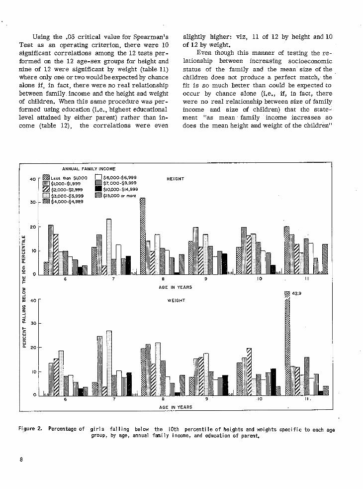
Using the .05 critical value for Spearman’s Test as an operating criterion, there were 10 significant correlations among the 12 tests per-formed on the 12 age-sex groups for height and nine of 12 were significant by weight (table 11) where only one or two would be expected by chance alone if, in fact, there were no real relationship between family. income and the height and weight of children. When this same procedure was per-formed using education (i.e., highest educational level attained by either parent) rather than in-come (table 12), the correlations were even

ANNUAL FAMILY INCOME

slightly higher: viz, 11 of 12 by height and 10 of 12 by weight.

Even though this manner of testing the relationship between increasing socioeconomic status of the family and the mean size of the children does not produce a perfect match, the fit is so much better than could be expected to occur by chance alone (i.e., if, in fact, there were no real relationship between size of family income and size of children) that the statement “as mean family income increases so does the mean height and weight of the children”

HEIGHT

AGE IN YEARSs s kl 40 WEIGHT

$ 3

2 30

!s z E p 20

0. 6 7 6 9 IO Il.

AGE IN YEARS

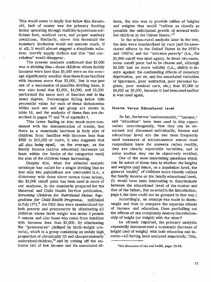
Figure 2. Percentage of girls falling below the 10th percentile of hei.ghts and weights specific to each age group, by age, annual family income, and education of parent,

8

describes the situation much more plausibly than the statement “there is no relationship between family income and height and weight.”

The weighted regression analysis described on pages 75-77 of appendix I produced similar results (tables 11,12). The slope of the line fitted through the mean heights (or weights) andthe mid-point of each income (or educational) level was tested to determine whether it differed statistically from a zero slope, i.e., no relationship at all between height (or weight) and income (or education.) Of the 12 times the line was fitted by

EDUCATION OF PARENT

height and the slope was determined and then tested for income groups, 10 of the lines were significantly greater than zero (p < .05) and when fitted by weight eight were significant. When these same tests were performed on the population grouped by educational level, 11 of 12 were significantly greater than zero both by height and by weight. If, in fact, there were no real relation-ships it would be expected by chance alone to find, on the average, only one slope in 20 significantly greater than zero at p< .05.

40 HEIGHT

0 6 7 8 9

AGE IN YEARS [email protected]

40 WEIGHT

AGE IN YEARS

Figure 2. Percentage of girls falling below the 10th percentile of heights and weights specific to each age group, by age, annual family income, and education of parent-Con.

9

Analysis by Smallest ‘IO Percent of Children _

Because of the increasing interest in population surveys that aim to assess the nutritional status of children, a separate.analysis was per-formed that focused especial attention on the smallest children in the population by height and/ or weight. Percent distributionsm were obtained for each of the 12 age-sex groupings for height and for each of those for weight (figure 2 and tables 13,14) and the first decile or the lowest 10th percentile by height and by weight was chasen as the center of the study. The data were arranged by, family income and educational groupings as before.

The height (and weight) value at the lowest 10th percentile, obtained for each age-sex group, was designated the cutoff point for that group. Then, for each of the 10 income (or eight educational) groups within each of the 12 age-sex groups, the percent of children falling below this value was correlated with family income (or educational level).”

Spearman’s rank correlation was performed on these percentages under the cutoff point as was done with the means (pages 5-9 of text and pages 74-7’5 of appendix I). The number of significant correlations as seenin table 15 was less than when

mIn the first report (page__-4), it was stated “It was assumed that the measurements-heights and weights-were distributed uniformly across each of the height and weight groups. On the basis of this assumption the linear interpolation method was used to derive bpth the height and weight percentiles. For both the heights and weights the Sth, lOth, 25th, 5Oth, 75th, 9Oth, and 95th percentiles were derived for each sex-age group.” On further examination, this assumption was quite incorrect. The measurements were not evenly distributed at the extremes. In fact, by actual calculatjon, several times this method produced only 2 and 3 percent of the population below the computed estimated 10th percentile. In the present analysis percentiles were computed by frequencies for each single centimeter group rather than a 5-centimeter group. This way the error by extrapolation cannot possibly exceed a centimeter; whereas in the other it exceeded 2 centimeters several times.

“As seen in table 13, since none of the percentages for the income group of less. than $500 were reliable by the criteria (described on page 73 of appendix I), the income group of less than $500 was pooled with the income group of less than $1,000 for analysis by separate age-sex groups. Similar pooling was not necessary for the analysis by educational level.

the means were compared (i.e., 10 of 12 by height and six of 12 by weight for income and nine of 12 by height and seven of 12 by weight for education); however, the sampling variability at the extremes of the distribution makes this type of statistical testing much more erratic.

DISCUSSION

The fact that there is a positive relation-ship between the socioeconomic status of the family, as determined in the Health Examination Survey, and the heights and weights of the children, i.e., in general, as income and educational level increase the physical size of the children, at ages 6-11, also increases, seems well established. This finding was not unexpected.

But what is the shape of this relationship? And what is its magnitude not only in terms of mere numbers but also when gauged by comparison with similar relationships from other studies? The behavior of the other variables-both dependent and independent-will also be examined. Various uses of the data will be suggested and discussed followed by speculation on the larger meaning of the present findings.

.Shape of Relationship . .

Preliminary inspection of the data had suggested that rather than a monotonic increase be-tween income (or education) on the one hand and height (or weight) on the other-as has beendemonstrated here-there was a major single step increase at about $3,000 (figure 3A rather than B). It was as if this jump were an identifiable threshold or critical level in terms of dollars.

Body Bodysize A size B

,I1 ,/ 0 $3,000-’ $15,000 0 $15,000

FAMILY INCOME

Figure 3. Concept of step function increasing function

10

This would seem to imply that below this thresh-old, lack of money was the primary limiting factor operating through inability to purchase sufficient food, medical care, and proper sanitary conditions. Similarly, above this threshold the monetary limitation would not operate much, if at all. It would almost suggest a simplistic solution: merely supply dollars and this “bad correlation” would disappear.

The present analysis confirmed that $3,000 was a dividing line-those children whose family incomes were less than $3,000 were on the aver-age significantly smaller than those from families with incomes more than $3,000. But it was just one of a succession of possible dividing lines. It was also found that $2,000, $4,000, and $5,000 performed the same sort of function and to the same degree. Percentages falling below 10th percentile value for each of these dichotomies within each sex and age group are shown in table 16, and the analysis of these data are de-scribed in pages 77 and 78 of appendix I.

This latter finding is also much more consistent with the demonstration of trends, that there is a monotonic increase in body size of children from families with incomes less than $500 to $15,000 or more. It also suggests that all else being equal, on the average, as the family income (and/or education) increases (at least within the limits of the categories used) the size of the children keeps increasing.

Despite this, when the selected analytic technique has called for a single dividing line so that only two populations are contrasted (i.e., a dichotomy with those above versus those below), the $3,000 cutoff point has been used in some of our analyses. In the standards prepared for the Maternal and Child Health Service publication, Screening Children for Nutritional St&us: Suggestions for Child Health Programs, published in July 1971,’ the HES data were standardized for both poverty and prematurity by eliminating all children whose birth weight was under 5 pounds 9 ounces and also those who came from families with incomes less than $3,000. By eliminating the “prematures” (defined by birth-weight criteria), which is a group containing an unduly high. proportion of chronically ill and also persistently undersized children:’ and by cutting off the extreme tail of low income and its associated ef

fects, the aim was to provide tables of heights and weights that would “reflect as closely as possible the anticipated growth of normal well-fed children in the United States.“’

In the urban-rural analysis later in the text, the data were standardized by race (and its associated effects in the United States in the 1950’s and 1960’s) and for “extreme poverty” (i.e., the $3,000 cutoff was used again). In these two cases, some cutoff point had to be chosen and, although $3,000 had no more validity (i.e., ability to in-sure against the confounding effects of monetary deprivation, per se, and the associated variables of ignorance, poor sanitation, poor personal hygiene, poor medical care, etc.) than $2,000 or $4,000 or $5,000, because it hadbeenused earlier it was used again.

Income Versus Educational Level

So far, the terms “socioeconomic,” “income,” and “education” have been used in this report rather interchangeably. Now they can be examined and discussed individually. Income and educational level are the two most frequently used measures of socioeconomic status: most respondents know the answers rather readily, they are clearly reportable variables, and in some studies they can be objectively verified.

One of the most interesting questions which can be asked of these data is whether the heights and weights (and hence, on a population level, the general health)’ of children more closely reflect the family income or the family educational level. (It would have been interesting to discriminate between the educational level of the mother and that of the father. But as noted in the Introduction, page 4, the data could not be grouped in that way.)

Accordingly, an attempt was made to disentangle and then to compare the separate effects of income and education. Does partialling out the effects of one completely destroy the relation-ship of height (or weight) with the other?

As already reported, the primary analysis repeatedly demonstrated a monotonic increase of height (and of weight) with both education and in-come-all having been analyzed separately. This,

%ee discussion of size and health, pages 25-28.

11

of course, could have a variety of meanings, the two extreme ones being: (1) Income and educational levels are two independent factors operating with about equal force or (2) income is the effective variable, but education and income are so highly correlated that education also demonstrates the same monotonic increase (and vice versa).

It’s so evident that income and education interact in so many ways that we know a priovi that neither extreme could be completely true. The first alternative can be rejected because in-come and education are anything but “independent factors.” And the more complicated second extreme alternative, if true at all, could be true only in ‘degree. The latter alternative would have been demonstrated analytically if partialling out the effects of one completely destroyed the relationship of height (or weight) with the other. But this was not at all the case:

Therefore, an intermediate relationship was sought: viz, acknowledging the high degree of interaction between income and education, when the effects are partialled out by holding one constant and observing the action of the other (as above), which one-education or income-has-the greater residual effect?

Rather than obtaining a clear-cut answer to this question, the data would yield only a hint.

Income is held constant by using only those people in the $S,OOO-$7,000range-this income group was chosen because it is large enough for analysis (N= 1652 1: it was the modal income group (table 1) in the United States in the early 1960’s; and it 3s clearly above a “poverty level”-and the educational trend is observed (tables 17,18). Then educational level was held constant by using only those who were graduated from high school but did not go to college (table 19). This is clearly the modal educational group and large enough for a “minimal analysis” (N=2750 1 and the height (and weight) trend by income was observed. Even though these two modal groups were the largest single groups among the HES data, in the tails of both distributions there are many extremely small cells and empty cells.

Spearman’s coefficients of correlation demonstrated no consistent trend over all age-sex sub-groups (table 20) as was demonstrated with our

total population. Four significant correlations were found when holding income constant, while only one was found when holding education constant. Although this gives a slight hint that education is a more important factor than’income in affecting the average size of children, it has certainly not been statistically demonstrated.

The comparative regression analysis was slightly more suggestive. When comparing the normalized magnitudes (z values) of the slopes of the fitted regression line of height (or.weight) versus income (table 11) to height (or weight) versus education (table 12), for each of ‘the 12 age-sex categories, it was found that education had the greater z values in eight of the 12’groups for weight and eight of 12 for height. By no means are these two analyses considered definite enough to claim as a finding; they ,are merely suggestive. (See discussion of sign test, page 74 of appendix -I>.

The most prudent conclusion is that income and education are so highly correlated andinteract in such a complex manner that a study must be specifically designed to tease out andisolate these two variables so that their modes of operation and their relative magnitudes of effect on the normal or healthy growth brocess of childrencan be studied with precision and with sufficientnumber of subjects to draw more definite conclusions. In a multipurpose cross-sectional study’such as the Health Examination Survey with so many variables being studied.and with a sample rep‘resentative of the total United States populationF one is left with-except for, perhaps, a hint that the educational level of parents affects normal healthy growth and development of the children slightly more than their income does-the rather inconclusive conclusion that education and income are simply separate measures of one conglomerate variable, “socioeconomic status,” as it affects, the size of children. .-

POn the one hand, this type of sample is absolutely necessary to accurately estimate the frequencydistributionof these biomedical parameters in the United States; but, on the other hand, when the data from this type ,of sample is used for hypothesis testirzg, subsamples must be selected which are-by the time all the necessary conditions and characteristics are met-of much stialler size than would be more readily attainable in a single-purpose epidemiologic study.

12

-- Other Variables

When looking both at the two dependent variables, height and weight, and at the biologicvariables used as the major population subgroupings for analysis (viz, age, sex, and race) little, if any, differences in response to socioeconomic effects can be detected within these contrasting sets of variables.

By careful inspection, the two principal de-pendent variables-height and weight-appeared to vary by socioeconomic status similarly to each other throughout all sex-age groups. In other words, they seemed equally sensitive to socioeconomic effects.¶

Again by careful inspection, heights and weights appeared to vary by socioeconomic status for the boys in the same way as for girls, for Negroes as for whites, and throughout the six different single-year age groupings.

It is reported by Acheson that the growth of boys is generally affected more by adverse environmental conditions than is that of girls and conversely, when favorable conditions are re-stored, that boys have more “catch-up” growth?“” This analysis of HES data can neither confirm nor deny this. Even though this differential was not observed, the cells are so small and the apparent magnitude of effects of socioeconomic deprivation on these grouped data is perhaps so slight that it is not a proper test of the above hypothesis.

It is stated also that children are more sensitive to adverse conditions during the most

PAnalogous to income and education as measures of socioeconomic status, it can be said that height and weight are simply the two most common and useful measures of the single dependent variable, “size.” In these analyses height and weight are not used as two variables independent of each other which, of course, they are not. However, when differences in size of children are used, as here, to examine differences in environmental circumstances-rather than comparative growth over t ime of a group of children from similar environments as would be found in the traditional child growth studies (in which the chief determinants of variation are genetic)-the two measures are more independent of each other (e.g., a fat boy in a circus versus the emaciated child in a war-ravaged country can be the same height and age).

The complex relationship between height and .weight will be examined further in future reports when additional body measurements are considered.

rapid periods of growth. The most likely ages to detect this, however, would be infancy and adolescence rather than the slower growth between 6 and 12 years. Furthermore, when analyzing for this effect, the data must be looked at in conjunction with skeletal age and other maturational measures so that, if an effect be found, it can be determined whether it be maturational delay or permanent stunting.

An analysis of trends was performed separately on whites and Negroes (tables 11, 12). Although a monotonic increase (identical to that demonstrated for all races combined) was found for “whites only,” the same results could not be demonstrated by use of the “Negro only” data. But rather than inferring that socioeconomic status affects the growth of black children differently from the way it affects the growth of white children, it must be noted (as reported on page 5) that the sample size of the blacks was less than one-sixth that of white children. There were about 80 Negro children within each of the 12 sex-age groups. After these 80 were distributed into 10 economic subgroups, many of the sub-groups did not contain any or contained only one or two subjects (table 1). The small cell frequencies necessitated collapsing the 10 income and educational categories into sometimes as few as four or five pooled categories because of the criteria explained in the appendix for determining the reliability of HES data. The nature of the Spearman correlation coefficient is such that smaller correlations will be found statistically significant if there are more degrees of freedom (i.e., a larger number of categories). This may explain why it was often impossible to demonstrate significant increasing trends with the collapsed Negro data. Even though the severe lim itation on the sensitivity of the test imposed by the sample size almost negates the attempted parallel analysis by race, there is no evidence, either within the HES data or fromother sources, to seriously consider the proposition that socioeconomic factors affect the growth (and health) of black and white children differently.

Urban-Rural Differences

In the monumental compendium, Growth of Man by Wilton Krogman, in the Tabulae Biologicae series in 1941:” in which summary tables

13

of all the data on human growth in the world literature between 1926 and 1938 are presented, there were only six studies (three, United States; one, England; one, Scotland; one, Swiss) which dealt in any way with urban-rural differences in the size of children. All of them were simply descriptive of the differences as found without any concomitant analysis of differences in socioeconomic status or ethnic composition. In the American studies, the urban children were distinctly larger (but the rural were rural Utah, the Eastern Tennessee mountains, and Puerto Rico) while in both Scotland and England the farm children were distinctly larger than the urban. The Swiss study which compared army recruits found that before 1910 the rural youths were much the larger, but by 1930 there was almost no detect-able urban-rural difference.

Since then Wolanski and associates13-15have been intensively comparing growth in Polish children (i.e., rates, attained size, and patterns of growth)between urban children and those from the fast disappearing medieval villages. They consistently find size and most measures of physiologic response superior in the urban children together with an earlier maturation. Although their data are extensive (including genetic studies) and their analyses are sophisticated, they have been unable to satisfactorily adjust for the accompanying great socioeconomic disparity be-tween village and city dwellers in Poland to measure the effect of urbanization per se on the growth of children.

This analysis of HES data is an attempt to make some contribution to the subject which can be very loosely stated, “In general, is country living more healthful for children than city living?” This loose question suggests many others like the following: “Does the boy who stays on the farm grow bigger and stronger than his cousin who moved into the city?’ and “Does the greater amount of fresh air [and outdoor living and exercise?]of the farm promote better growth?“; “For parents who are keenly interested in these kinds of questions-and at the same time have the ability to make the choice-is it better to raise their children in the city or in the country?’

When trying to get at some ofthesequestions with these HES data, a variety of ways of grouping and organizing the data have been attempted.

As pointed out on page 4, biologic epidemiologic sense had to be made within the given classification system. Page 81 of appendix II gives the coding definitions in more detail and also lists the names and populations of the 24 SMSA central cities that constituted the HES sample of cities. Within the city limits of these 24 places there are shared in common most of the following: heavy industry; commerce; high population density; air and noise pollution; automobile traffic; diversity of entertainment attractions; lack of open space; plethora of asphalt, concrete, and brick rather than vegetation; broad population mixture of various ethnic and socioeconomic groups; and many cultural and educational opportunities. There are also sophisticatedmedical centers in most of them, complex and active health departments, and more consistently safe drinking water and waste disposal available almost automatically to every member of the community regardless of geographic section or socioeconomic stratum than in rural areas with their overflowing septic tanks, privies, erratic refuse disposal systems, individual water sources, et$

Using the dichotomy SMSA/not-SMSA, SMSA is further subdivided into: central city/not central city. Central city is a much more definable population and much more homogeneous in character than is SMSA/not central city. Although, generally, SMSA/not central city is “suburbia” and all that goes with it, it ranges from the highly industrialized Wyandotte-Ecorse section of the Detroit SMSA to Gibson Island, Maryland, or North Shore Long Island, New York.

The other side of the dichotomy not-SMSA, includes most’ of the urban but small cities, towns, and villages under 50,000 population on the one hand and almost all’ the frankly rural on the other. Rural is further subdivided into farm and nonfarm. The farm population is de-fined as all persons living in rural territory in places of 10 or more acres from which sales of farm products amounted to $50 or more during the preceding 12 months or on places of less than 10 acres from which sales of farm products had amounted to $250 or more during the preceding 12 months (appendix II, page 81).

*Many small urban cities have been included as part of an SMSA and 1-2 percent rural, including farms, will also fall in SMSA.

14

To increase the sample size, both farms over 10 acres in size and those under 10 acres were combined into one group. But this shouldn’t create too much heterogeneity in the group for analysis because both populations were standardized by race and income. The rural nonfarm category was discarded because it was sucha heterogeneity, as the Park Ranger’s House in Yosemite and large estates on Long Island to shacks in the deepest recesses of Appalachia and mud huts in the sands of Southern Texas.

By standardizing for race and major in-come break (i.e., less or more than $3,000) and using the two most homogeneous and yet contrasting groups-contrasted by degree of urbanization-an attempt is made to partial out the effects of “urbanization” itself on heights and weights of children.

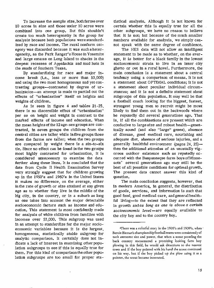
As is seen in figure 4 and tables 21-25, there is no discernible effect of “urbanization” per se on height and weight in contrast to the marked effects of income and education. When the mean heights of the 12age-sex groups are contrasted, in seven groups the children from the central cities are talley while in five groups those from the farms are taller; when the two groups are compared by weight there is a six-to-six tie. Since no effect can be found in the two groups most highly contrasted for urbanization, it is considered unnecessary to examine the data further along these lines. It is concluded that the data from Cycle II Health Examination Survey very strongly suggest that for children growing up in the 1950’s and 1960’s in the United States it makes no difference, on the average, either in the rate of growth or size attained at any given age as to whether they live in the middle of the big city, in the country, or in a suburb as long as one takes into account the major detectable socioeconomic factors such as income and education. This statement is most confidently made for analysis of white children from families with incomes over $3,000. This subgroup was used in an attempt to standardize for the major socioeconomic variables because it is the largest, homogeneous, statistically stable subgroup for analytic comparison. It certainly does not indicate a lack of interest in examining other population subgroups to see if this is equally true for them. For this kind of comparison the other population subgroups are too small for proper sta

tistical analysis. Although it is not known for certain whether this is equally true for all the other subgroups, -we have no reason to believe that it is not; but because of the much smaller numbers avaiIable for analysis, we simply can-not speak with the same degree of confidence.

The HES data will not allow an intelligent statement to be made as to whether, on the aver-age, it is better for a black family in the lowest socioeconomic strata to live in an inner city ghetto or out in a rural hovel. Furthermore, the main conclusion is a statement about a central tendency using a comparison of means. It is not a statement about OPTIMAL conditions; it is not a statement about peculiar individual circumstances; and it is not a definite statement about subgroups of this population. It tiay well be that a football coach looking for the biggest, fastest, strongest young men to recruit might be most likely to find them out in the backwoods where he reputedly did several generations ago. That is, if all the combinations are present which are conducive to large size and robust health-genetically sound (and also “large” genes), absence of disease, good medical care, nourishing and adequate diet, absence of serious injuries, and a generally healthful environment (pages 24, 25)then the additional stimulus of an unusually vigorous outdoor existence such as reputedly occurred with the Bunyanesque farm boys of Minnesota’ several generations ago may still be the best of all possible conditions for optimal growth. The present data cannot answer this kind of question.

The main conclusion suggests, however, that in modern Americq, in general, the distribution of goods, services, and information is such that good food, good medical care, and general healthful living-to the extent that they are reflected in growth andas long as one is ahovea Ce-hin

socioeconomic level -are equally available to the city boy and to the country boy.

flhere was a colorful story in the 1920’s and 1930’s, when * Bernie Bieman’s championship football teams were consistently of such awesome size and power, that when a scout prowling the back country encountered a promising looking farm boy plowing in this field, he would ask directions to the nearest town and if the boy pointed with his hand the scout continued on his way, but if the boy picked up the plow using it as a pointer, the scout became interested.

15

BOYS GIRLS 150 r INCOME $3.000 OR MORE 150 r

Rural farm

Central CitdSMSA

rOL 0

6 AGE IN YEARS AGE IN YEARS

z 30 30 2” s x z 20 20

5” ci 3 IO IO

0 0 6 7 B 9 IO II

AGE IN YEARS AGE IN YEARS

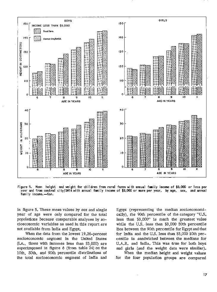
Figure 4. Mean height, and weight for children' from rural farms with annual family income of $3,000 or less per year and from central city/WA with annual family income of $3,000 or more per year, by age, sex, and annual family income.

Comparison With Other Populations

To achieve a sense of scale, to better appreciate the magnitude of the differences of the contrasting socioeconomic groups, the HES data have been plotted against data from other population groups around the world and also against the “secular trend” of North America.

McDowell et al. compared the mean heights and weights of children 6 through 11 years of age from the United states, United Arab Republic

(U.A.R.), and IndiaJ7 As described in the report, the sources of data were the following: the U.S. data were the same HES material presented earlier by age, sex, and race by Hamill’ et al.; the data from India were from anationwide krosssectional survey conducted from 1956-65 by the Indian Council on Medical Research; those from Egypt were .from a national school health survey in 1962 and 1963 jointly conducted bytheEgyptian Central Statistical Committee and the Ministry of Public Health. The comparison,is reproduced

16

BOYS I- GIRLS

INCOME LESS THAN $3,000

-I-

iia ,-Ir-

6 7 8 9 IO II 6 7 8 9 IO II


40

10

0 6 7 6 9 lo II 6 7 8 9 IO II


Figure 4. Mean height and weight for children from rural farms with annual fmily income of $3,000 or less per year and from central city/SiSAwith annual family incane of $3,000 or more per year, by age, sex, and annual family income.-Con.

in figure 5. These mean values by sex and single year of age were only compared for the total populations because comparable analyses by socioeconomic variables as used in this report are not available from India and Egypt.

When the data from the lowest 19.26-percent socioeconomic segment in the United States (i.e., those with incomes less than $3,000) are super imposed in figure 6 (from table 24) on the lOth, 5Oth, and 90th percentile distributions of the total socioeconomic segment of India and

Egypt (representing the med ian socioeconomitally), the 90th percentile of the category “U.S. less than $3,000” is much the greatest value while the U.S. -less than $3,000 50th percentile lies between the 90th percentile for Egypt and that for India and the U.S. less than $3,000 10th percentile is sandwiched between the med ians for U.A.R. and India. This was true for both boys and girls (and the weight data were similar).

When the med ian height and weight values for the four population groups are compared

17

--

HElGt HEIGHT WEIGHT WEIGHT(cm8 (b

150 50

- U.S. boys~~*m~rn~~mmwt~lJ.S girls ..-mm.= U.A.R boys -z- U.A.R girls I-I mm---.

India boysIndia gir4s

I I 6 7 8 9 IO II 6 7 8 9 to II


Figure 5. Mean height and weight for children, by sex and single year of age: United States, United Arab Re-public, and India.

150 - GIRLS

140 ‘-

B 130 -? E E g l20-

1

5 p IIO-

100 -

I I I I I I 6 7 8 9 IO II 6 7 8 9 IO II


Figure 6. IOth, 5Oth, and 90th percentiles of height and weight for U.S. children with annual family incomeless than $3,000 per year, U.A.R. children, and Indian children, by age and sex.

18

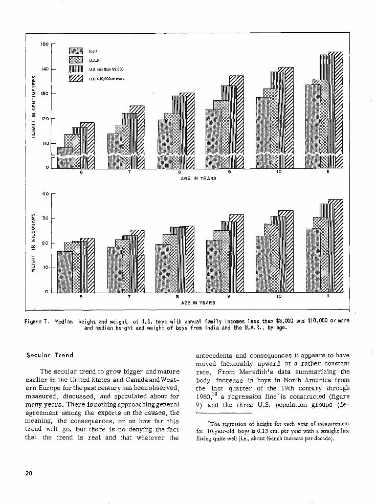
(viz: India, Egypt, U.S. less than $3,000, and U.S. more than $10,000) it is seen in figure 7 that there is less difference in children’s sizes between the two socioeconomic extremes in the United States than between the children from the U.S. less than $3,000 and the median of Egypt. (When ranking the countries around the world by technological and socioeconomic development, Egypt is certainly not one of the most “under-developed.“)

Report No. 104 referred to Meredith’s collation of the world literature on heights and weights of children in which he uses 8-year-olds as the reference age in over 300 samples.r8As he points out in comments about eachstudy, there is a great range in the precision and accuracy of the data.

In figure 8 the three U.S. population groupings (i.e., less than $3,000, more than $10,000, and all incomes combined) are placed on a continuum from around the world. Although it would

60 - BOYS

90th-50th. . . . . . . . . . . . IOU,----.

50 -

6 7 8 9 IO II AGE IN YEARS

be a mistake to expect too much accuracy from. _ some of these data, a comparative scaleofvalues can be readily appreciated.

Another way of assessing the magnitude of difference between the extreme socioeconomic levels is that, when comparing mean heights, children from the upper income stratum are about 0.4 years “ahead of’ those from the lowest level (A of table 25). Specifically, a lo&year-old boy (U.S. less than $3,000) has the same average height as a boy 10.02 years (U.S. more than $10,000).

Comparing countries in B and C of table 25, U.S. children’s heights are about 1.58 years ahead of their U.A.R. counterparts and 2.16 years ahead of their Indian counterparts. Specifically, a 10.5-year-old boy from Egypt has, on theaverage, a height equivalent to a boy 8.8 years from the United States; while the 10.5-year-old boy from India is equivalent in height to an 8.28-year-old boy from the United States.

GIRLS

L I I I I I 6 7 8 9 IO II

AGE IN YEARS

Figure 6. IOth, 50th, and 90th percentiles of height and weight for U.S. children with annual family incomeless than $3,000 per year, U.A.R. children, and Indian children, by age and sex-Con.

19

U.S. less than $3,000

U.S. 510,000 or more

AGE IN YEARS

40

0 6 7 8 9 IO II

AGE IN YEARS

Figure 7. Median height and weight of U.S. boys with annual family incomes less than $3,000 and $10,000 Or-more and median height and weight of boys from India and the U.A.R., by age.

Secular Trend

The secular trend to grow bigger andmature earlier in the United States and Canada and West-ern Europe for the past century has been observed, measured, discussed, and speculated about for many years. There is nothing approaching general agreement among the experts on the causes, the meaning, the consequences, or on how far this trend will go. But there is no denying the fact that the trend is real and that whatever the

antecedents and consequences it appears to have moved inexorably upward at a rather constant rate. From Meredith’s data summarizing the body increase in boys in North America from the last quarter of the 19th century through 1960: ' a regression linet is constructed (figure 9) and the three U.S. population groups (de

*The regressionof height for each year of measurement for lo-year-old boys is 0.13 cm. per year with a straight line fitting quite well (i.e., about %-inch increaseper decade).

20

HEIGHT IN CENTIMETERS

Figure 8. Relation of heights of three U.S. income groupings of 8-year-old boys to those of rest of world, viz, Meredith Study.

fined socioeconomically) are placed on it. Using this regression line as another way to scale the magn itude of differences, the U.S. socioeconomic extremes are only about 14% years apart (i.e., U.S. less than $3,000 plots at 1961 and U.S. more than $10,000 plots at 1975), while Egypt plots at about 1901 and Indiaat about 1878).

Whatever the causes leading to this secular trend in the Western World (see discussion of con-founding variables, pages I3 and 14 of Report No. 104) the effective complex of factors appears to be intimately bound up in the “Western style of life” rather than a geographic region oftheglobe, viz, Australia and New Zealand: Northern and Western Europe; United States and Canada; and, increasingly, Japan and probably U.S.S.R. (also see discussion, Report No. 104, pages 15 and 16, American Negroes versus African Negroes). Furthermore, there appears to be a gradient of sizes roughly corresponding to the degree of “Westernization” (figures 8 and 9). Among the companions to this increasing size and earlier age of maturation of children are greatly lowered maternal and infant deaths, lower mortality and morbidity of childhood, and greatly increased life expectancy.

In searching the available data for the ma in causes of this increasing size of children, none clearly stand out. There were certainly no simple explanations apparent. That it is not simply due to a rising educational level (e.g., more people going to college each year) or income level (e.g., constantly rising gross national product (GNP))” or elevated socioeconomic status, is suggested by the following two arguments:

(1) Hathaway in 1960 reviewed the available data from over 20 U.S. college studies, covering the previous 100 years.?OTable A summarizes two of the most extensive studies. Most of the studies compare incoming freshmen over the years. Although there are, naturally, some differences in actual measurement, they are all unanimous on their findings: i.e., incoming freshmen have be-come taller and heavier (despite also becoming approximately 1 year younger) over this time. This is equally true for women and for men. The sources of the most extensive serial data were Harvard, Yale, and Amherst for men and We llesley, Smith, and Vassar for women. The magn itude of change was roughly 3 inches in height

‘But it is believed, see page 24, that the very complex “increased standard of living” does encompass a large part of the factors, but that it is not primarily the money itself (or even the GNP part, itself).

21

105 I I I I I I I I I I 1870 1880 1890 1900 1910 1920 1930 1940 1950 1960 1970

IO YEAR OLDS

Figure 9. Regression line showing the growth of U.S. IO-year-old children during the last century by income groups, with the comparison of Indian and U.A.R. children, for the years 1963-65.

and over 20 pounds in weight.” Analysis for percentage of tall men (72 inches and over) in the freshman class support this. “At Amherst only

“This is only about 60 percent as great an absolute increase in size as Meredith estimated for IO-year-olds over the same time frame. And it is even a smaller proportionate increase for this disparity. Two explanations come to mind: part of the increased size in “Meredith’s IO-year-olds” might well be due to earlier maturation** and the other might be due to rising socioeconomic level of a greater proportion. That is, the college students would have rather constantly, over the 100 years, come from the highest socioeconomic strata-i.e., no relative change-whereas the much broader socioeconomic spectrum of Meredith’s IO-year-olds, it can be conjectured, might allow for a greater relative improvement over the years in the lower socioeconomic strata.

one class before 1910 had as many as 10 percent tall men; from 1937 all but two classes had over 20 percent tall men; and in 1956 and 1957 tall men made up over 30 percent of the class.“20There was a similar phenomenon at the other schools. And family comparisons of pairs of fathers and sons and mothers and daughters measured at the same age, i.e., when they entered as fresh-men-showed the sons to be almost 1% inches taller than their fathers had been and the daughters more than 1 inch taller than their mothers. Furthermore, table B shows that the total height difference between the first and fourthgeneration of Harvard men was 3 inches.

In short, this steady increase in the size of college students occurred within,. presumably, a

22

---

Table A. HARVARDMEN AND WELLESLFXWOMEN: Averaze heizhts and weixhts bv decades of birth, 1836-1915 -- -r Harvard men r . Wellesley women

Birth date Cases Height Weight Cases Height Weight

Number Inches Pounds Number Inches Pounds

1836-45---- 2 67.1 140.0 1846-55- 43 68.5 140.6 1856-65---- 335 68.1 138.4 45 63.3 119.9 1866-75---- 506 68.7 139.7 235 63.3 120.4 1876-85---- 307 69.1 146.8 212 63.7 120.7 1886-95---- 267 69.4 149.2 40 64.3 121.6 1896-1905-- 607 69.8 148.9 266 64; 6 123.7 1906-15---- 546 70.1 149.0 267 65.0 125.2

Source: U.S. Department of Agriculture, Heights and Weights of Adults in the United States by M.L. Hathaway and E.D. Foard, Home Economics Research Report No. lO,Washington, U.S. Government Printing Office, Aug. 1960, p. 28.

Table B. HARVARDMEN: Average heights and weights of fathers and sons,four generat Ions

AgeGenera- when

tion meas- Cases Height Weight ured

Years Number Inches Pounds

Great grand-fathers-- 50 8 67.0 149.5

Grand-fathers- - 30 92 68.6 152.4

Fathers--- 19 132 69.0 145.8 Sons----..- 18 153 70.1 151.1

Source: U.S. Departmentof Agriculture,Heights and Weightsof Adultsinthe United States by M.L. Hathaway and E.D. Foard,Home Economics Research Report No. 10,Washington, U.S. Government Printing Office, Aug. 1960, p.38.

stable socioeconomic stratum without change in “income” or "educational" levels or socioeconomic status.

By “stable socioeconomic stratum” is noP meant the relative constancy of the constituent families such as existed in England for 9OOyears; but instead the relative socioeconomic stability over time of the population channel, itself, from which the students were drawn. (This is conjecture; the authors could findnodefinitive studies of the two following assumptions: viz, (a) the educational and relative income constancy over the century of the higher socioeconomic level families-but certainly from 1860 to 1960 in America, the carpenter’s way of life changed far greater than did the physician’s-and (b) the college students, but most especially the Ivy League students, were predominantly selected from this channelWduring the century.)

Wit has only been since 1945 that the U.S. college population has been originating f%om an ever-broadeningsocioeconomicandculturalbase.

23

(2)When contrasting the two United States socioeconomic extremes, there appears to be an enormous disproportion between the rather small differences in the size of the children on the one hand and the magnitude of the differences in income and educationon the other. For example, when the regression line constructed for secular trend of increasing size is used for a sense of scale, it was shown (figure 9) that the children of the two extreme groups were only 14.6 years apart. That is, if the trend continues without drastic change, in about 10 or 20 years the mean heights of the children from the lowest socioeconomic one-fifth will equal the mean heights today of the children from the upper group. Are there the slightest grounds for predicting that in this

. same 10, 20, or even 50 years the real income of this same segment of the U.S. population receiving less than $3,000 annually (median betvOeen $1,000 and $2,000) will have equalled today’s real income of the segment representing $10,000 or more (median near $14,000)? And even less likely would be the bridging of the formal educational disparity: viz, the lowest 19.26-percent income represents educationally 9th and 10th grades and below with a median between the 7th and 8th grades, while the comparable upper educational segment had a median of 4 years of college!

Although classifications of heights and weights of children by socioeconomic levels similar to these HES data are not available from other countries which would permit precise comparisons,, figures 5-9 give enough sense of scale to strongly suggest that more of the factors conducive to greater size of children are available to the lowest socioeconomic groups in the United States than to all but the most highly favored few in India and to no classes at all in the under-developed countries such as Burma and Ethiopia. Although income and education make a very demonstrable difference, the other factors which are universally available to all classes of Americans make far more difference. (This finding does not repudiate the statements of the past few years concerning “pockets of hunger and starvation” in the United States. It does, however, emphatically limit these pockets in size, in number, and in severity. Otherwise one would be forced to conclude that the nonstarving pro-portion of the lowest socioeconomic group in the

United States yields children much bigger than the next higher socioeconomic groups to be able to maintain soup avWa@s of height and weight only very slightly lower than those of the next higher socioeconomic groups.

In addition, if the same socioeconomically lowest one-fifth of the U.S. population is still so much larger than the national averages of so many other countries (figure 8) and if included in that group werea large proportion of severely stunted, malnourished children, then how gargantuan, indeed, must be the remaining portion to pull the average sizes of this lowest U.S. socioeconomic group so much higher than the figures from most of the rest of the world. To repeat, this argument does not claim that the HES data prove there are no pockets of malnutrition and even starvation in the United States of America; but it does greatly limit their possible extent.)

The HES findings also strongly suggest that a shift in the population from rural to urban-if it occurs in a society like mid-century U.S.A. in which both farms and cities are “modern” (page 15)--does not explain the secular trend of increasing size. The HES findings by themselves cannot, of course, shed light on the effects on children’s growth of the steady move from rural America to urban America of the past century. However, the very convincing college data referred to on pages 21 and 22 of steadily increasing size despite the trend of the Ivy League schools to draw students from ever-widening socioeconomic and geographic regions over this same century (again, authors’ conjecture) seem convincing that the shift in America from farm to city could not, in itself, explain much of the secular increasing size.

Milicent Hathaway and Elsie Foard concluded the discussion of their two remarkably wide-ranging and thoughtful r eports20*“Twith the following: “Many factors are doubtless responsible for changes in body size of the population of the United States. Although there is still disagreement among scientists as to the limits of plasticity of the human organism, changes in size represent an increase under more favorable environment of the growth potential inherent in the genes (Gold-stein 1943 and Kaplan 1954). Some of these environmental factors are improvement in the socioeconomic status of much of the population,

24

improvement in medical care and sanitation, greater availability and consequent consumption of nutritious foods, and improvement in the general knowledge of nutritional needs.

“Improved prenatal and infant care has greatly reduced infant mortality. Attention to the care of infants and children through periodic examinations by family physicians, pediatricians, or at well-baby or child clinics is now practiced widely. The child has better dietary direction, immunization against childhood diseases, and early detection and correction of remediable conditions. More attention is given to outdoor play, and light sanitary homes are more generally available. This better start has contributed to better development, greater size, and longer life” (pages 99 and 100, reference 20).

The HES findings contradict nothing at all of what Hathaway and Foard stated in 1960. On the contrary, within the HES data, there were detected no simple, persuasive, and powerful factors which could be readily measured in a large nationwide survey and which, by themselves, directly accounted for most of the secular in-crease. Most of the increase is undoubtedly caused by the general complex of factors cited above by Hathaway and Foard that have all been part of the cultural-technologic transformation-urban and rural-in the past century in the United States.

Genetic Factors

Hathaway and Foard continued:“” “A major difficulty in studies of growth and size still is separationof such factors as accelerated maturation and genetic diversification from serial change6 produced by introduction of newer ethnic strains (Hunt 1958), a6 well as the effects of the many environmental factors” (page 100).

The confounding variable of accelerated maturation ha6 been frequently mentioned in Re-port No. 104 and earlier in this report and will be discussed in detail when data on Skeletal maturation are presented. This report has focused almost exclusively on socioenvironmental factor6 which may influence growth and size-and it is further limited to only those factors available in Cycle II. However, that does not signify that the authors totally disregard the importance of

possible genetic factors in addition to these environmental factors in this discussion of the meaning and causes of difference6 in children’s sizes both in the present and over the past.

The introduction of newer ethnic strains (so-called hybrid vigor) as discussed by Hunt22 and by Hathaway and Foard2’may explain some part of the secular trend; while social stratification of genes and assortative mating may ex-plain some part of the observed difference6 in the HES socioeconomic groups. (If, for example, social stratification had resulted in dissimilar frequencies of gene6 for size among differing socioeconomic levels, the result would be seen in differences among the offspring. Any genetic differences existing through the socioeconomic continuum would be intensified by positive assortative matingF3 i.e., the tendency for individuals to marry someone like themselves. This ha6 been observed, for example, for educational attainment.“* Despite the existence of some interclass mobility, assortative mating may ex-plain a portion of the observed differences.)

In Cycle III, concluded in March 1970, many genetic markers-principally on blood-were obtained on youths 12-17 years of age. These data, together with a special subgroup of several hundred twins from Cycles II and III, analysis by other nontwin siblings, and the fact that approximately one-third of the subjects examined in Cycle III were examined about 3 years previously in Cycle II (as 9 through 11-year-olds), will all be used in future report6 to enlarge this discussion of “possible causes” by the examination of genetic and other familial factors.

Size and Health

There has been throughout this entire discussion an implicit assumption that large size of children and health are so closely related that large size almost means good health. The most immediate distinction to be kept in mind when examining this relationship more Carefully is whether the subject is the individual child or a popuZution made up of individual children (or, more strictly, a sample representing a defined population of individual children). Then, the various meanings of the terms “size” and “health” bear further scrutiny in this context.

25

If when considering the meanings of “health,” the definition of the World Health Organization is used, “a state of complete physical, mental and social well-being and not merely the absence of disease or infirmity,” it would be well to amplify on the “absence of disease or infirmity.” For children, absence of disease should include not only overt but also latent disease such as Huntington’s chorea. It could also include precursors to later disease such as obesity, elevated blood pressure, and high serum lipids as well as behavior which fosters later ‘disease such as zigarette smoking and the reckless use of alcohol and other drugs. Absence of infirmity could be expanded to include freedom from transmissible genetic defects and developmental defects; good relative resistance to disease both during childhood and later life; enough vigor for enjoyment of pleasures and for effective work, study, and psychic growth; adequate physiologic and somatic development; and an environment conducive to growth. These seem to be the minimal preconditions for the rather expansive, “state of complete physical, mental and social well-being.” These criteria of health are as applicable to individuals as to a defined population, but, of course, the assessment techniques are quite different. The health assessment of the individual child is, of course, performed by the pediatrician, while that of the population is per-formed by the epidemiologist who synthesizes information and skills from the clinic, from surveys, and from vital and health record systems and relies on statistical analytic tools.

Just as the health assessment of the child is clinical while that of the population is epidemiological-with differing techniques, purposes, and emphasis but with much overlap-so the appraisal of size differs by subject (i.e., individual ‘or population) and purpose.

An appraisal of the size of the individual child-whether the main purpose be clinical or nonclinical-requires some understanding of his life context and enough information over time-either by repeated visits or by reliable history-to c,onstruct, at the minimum, a rudimentary growth curve. If the appraisal is for other-than-health reasons, it usually leans heavily to matters of taste, life style of family, and the individual’s abilities and ambitions. For example,

if a child is at the 99th percentile ift height,’ some of the most important questions to answer before a value judgment can be made are: Is weight proportionate? A boy or a girl? What shape growth curve? Any health significance? If these answers are happy ones, then an apprais.al moves into the more personal sphere: e.g., if he plans to become a professional football player, this can be very good, in general; however, if she had her heart set on becoming a jockey or ballerina it can be very discouraging, indeed. When relating size to the individual, there’s a .very clear distinction between the maximal and the optimal.

The clinical appraisal of size (or better, growth) has two aspects: (1) a suspected disturbance of size itself (or a desired alteration in projected size, such as when an unusual height for a girl is predicted) which is best performed at rather ,highly specialized growth centers if medical or surgical intervention is anticipated and (2) consideration of size in the clinical practice of pediatrics in which height and weight (including both a growth curve and recent changes) are usedas indicators of healthy or morbid processes.

In general, the common medical condition, obesity (which will be dealt with in a future report), and the much rarer condition, gigantism (excessive growth of the skeleton), are the only important medical conditions of excessive size. By “imp,ortance” is meant of sufficient prevalence to occur more than once or twice in an entire career in general pediatric practice or to have any impact on population data. Because almost all other medical disturbances of size-either of endogenous or exogenous origin-with the exception of obesity, result in low weight and/or low stature, “big” and “healthy” are linked together in common usage as in “big, healthy baby” or “big, strong, healthy boy.”

As assessing the meaning of a child’s size in terms of health is the function of the pediatrician-and in rarer cases pediatricians who specialize in disturbances of growth-so the assessment of the meaning of the size of children in a given population in terms of health is the function of the epidemiologist. The clinical assessment of size is completely described in a combination of the following four books along

26

‘

with a standard text like Nelson’s Pediatrics:25 Endocrine and Genetic Diseases of Childhood by Gardner,26 Growth and Development of Children by Watson and Lowry,27Pveventive Pediatrics by Harper!O and Growth-at Adolescence by Tanner?” (The books by Harper and by Tanner are good bridges between the clinical and the epidemiologic assessments.)

The only immediate contribution to the clinical evaluation which this report can make are a few additions to the following summary paragraph from Report No. 104 (page 16). “When applying these data to the individual child, one must use skill and additional specific knowledge about the child and his total setting. The size of parents

2fPCi region of country, so-and grandparents,‘ - **31-:32 cioeconomic strata, ethnic and racial differences (including the difficult assessment3%“‘30ffood in-take patterns from birth onward, which will vary by cultural habits and tastes, knowledge of nutrition, economics and availability of various foods), genetic differences, amount and type of exercise, disease, and environmental influences must all be used to make proper adjustments.”

Predictions or expectations about an individual are made by matching the one against a “similar enough group”’ for which percentage distributions are available for the given variable under study. It is then seen where the individual is placed with respect to all other “similar enough” individuals. This is a topographic activity. In Report 104, race (i.e., white or Negro) was found to make a real but so slight a difference that different sets of standards were not recommended, and children from the Midwest and Northeast tended to be a little larger than children from the South and West. Which sex made much more difference than race or region; but of course age was so important that the height or weight of a child without accounting for ageis almost meaningless.

In this report it has been shown that in the 1960’s degree of urbanization, per se, makes no

XOf course, the skill involves matching with a “similar enough” group except for the one variable under consideration and then not being a slave to a mechanical interpretation of the percentiles.

difference in a country like the United States. Income and education make a very real difference, but only a difference of a few percentage points . which was very small, indeed, when compared with the difference made by country of origin. By far the greatest difference in the size of children at a given age is made by how culturally and technologically similar the child’s country of origin is to the United States.

An epidemiologic assessment of the meaning of children’s size in a given population is what has been going on in this report (as a continuation of Report No. 104). A thorough assessment being beyond the scope of this one report, the focus has been on socioeconomic and demographic factors. As was stated when considering medically caused disturbances of size, obesity is the only “disease” of oversize of sufficient prevalence to affect population data. (This will be the subject of a future report.) Both clinically definedmedical conditions and epidemiologically defined conditions of large populations such as contagious diseases; community-wide sanitary and housing conditions; frequency of disease in the population, especially intestinal infestations; adverse climate; and-assuming increasing worldwide importance-community-wide nutritional circumstances and dietary practices all conspire to small size if they have an effect on size at all. Superimposed on these environmental conditions are the social, cultural, and economic capabilities not only of the community but also of the constituent families. Deficiencies in any of these spheres can all interfere with the full realization of the growth potential of the children.

Consequently in the 1970’s it seems most prudent to assume that for comparing large populations of children “the bigger they are the healthier they are” is a good rule of thumb with, of course, several qualifications.Y In fact there are some who feel that possibly all major population groups of the world are of the same po-

Y (1) Either the obese part of the population be considered separately or stature be considered the predominant index of size and (2) the population be representative of a large enough gene pool to compensate for some of the breeding groups knowr for unusual size like the Pygmy and the Watusi.

27

tential mean size genetically and that any diminution in size of the group mean is a direct measure of some adverse growth condition, Of course many who deal with population genetics do not agree but feel that while environmental circumstances certainly play a very large role in the resultant group sizes, the different large breeding groups of humans (races?) would still have their own distinctive sizes and shapes for the group as a whole even if all the environmental conditions which affect growth and health were somehow standardized throughout the world.

Despite the myriad complications when at-tempting to interpret causes and consequences in the accumulating growth data and despite the levels of sophistication used, Meredith nicely summarized the contrasting size of 8-year-old children around the world by statingJ8 “Norwegian children living in Oslo and Bergen had a mean body weight greater than that of [Pakistani] children living in East Pakistan by 21 pounds or 55773.”No one can doubt that, in this context, height and weight have a very profound relation-ship to any concept of “healthy children.“.

REFERENCES

INational Center for Health Statistics: Height and weight of children, United States. Vital and Health Statistics. PHS Pub. No. lOOO-Series II-No. 104. Public Health Service. Washington. U.S. Government Printing Office, Sept. 1970.

2NationaI Center for Health Statistics: Plan and initial program of the Health Examination Survey. Vital and Health Statistics. PHS Pub. No. lOOO-Series l-No. 4. Public Health Service. Washington. U.S. Government Printing Office, July 1965.

3NationaI Center for Health Statistics: Cycle I of the Health Examination Survey: sample and response, United States, 1960-1962. Vital and Health Statistics. PHS Pub. No. lOOO-Series ll-No. 1. Public Health Service. Washington. U.S. Government Printing Office, Apr. 1964.

4National Center for Health Statistics: Plan, operation, and response results of a program of children’s examinations. Vital and Health Statistics. PHS Pub. No. lOOO-Series l-No. 5. Public Health Service. Washington. U.S. Government Printing Office, Oct. 1967.

STanner, J.M., Hiernaux, J., and Jarman, S.: Growth and Physique Studies in IBP Handbook No. 9. Human Biology: A Guide to Field Methods, Weiner, J. S. and Lourie, J. A. London. Internat. BioI. Programme, 1969.

6Tanner, J. M.: Personal communication. 7Krogman, W. M.: A handbook of the measurement and

interpretation of height and weight in the growing child. Monog. Sot. Research in Child Dev. 13:(3), 1950.

*Standard Metropolitan Statistical Areas: Prepared by the Office of Statistical Standards, Bureau of the Budget. Washington. United States Government Printing Office, 1967.

YScreening Children for Nutritional Status: Suggestions for Child Health Programs. Public Health Service Publication, 1971.

loHarper, P. A.: Preventive Pediatrics: Child Health and Development. New York. Appleton, 1962.

llAcheson, R. M.: Effects of Nutrition and Disease on Human Growth, J. M. Tanner, ed., Human Growth, Vol. III of Symposia of the Society for the Study of Human Biology.. London. Pergamon Press, 1960.

12Krogman, W. M.: Growth of Man, in Denzer, H.; Koningsberger, V. J.; Vonk, H. J., eds. Tabulae Biologicae, Vol. XX. Don Haag. Vitgeverij Dr. W. Junk, 1941.

13 Wolanski, N. and Lasota, A.: Physical development of countryside children and youth aged 2-20 as compared with the development of town youth of the same age. Zietschrift Fur Morphologic and Anthropologie 54:272-292, Jan. 1964.

*4Wolanski, N.: Environmental modification of human form and function. Ann. N.Y. Acad. of Sciences 134~826, 1966.

1 SWolanski, N.: Formation of typology and body posture in town and rural. Acta Anatomica 56: 157-183,1964.

leWolman, A.: Personal communication. 17NationaJ Center for Health Statistics: Height and

weight of children in the United States, India, and the United Arab Republic. Vital and Health Statistics. PHS Pub. No. lOOO-Series ~-NO. 14. Public Health Service. Washington. U.S. Government Printing Office, Sept. 1970.

l*Meredith, H. V.: Body size of contemporary groups of eight-year-old children studied in different parts of the world. Monog. Sot. Research in Child Dev. 34-125:(l). Chicago. University of Chicago Press, 1969.

19Meredith, H. V.: Change in stature and body weight of North American boys during the last 80 years, in L. Lipsitt and C. Spiker, eds., Advances in ChiZd Develop&W and Behavior, Vol. 1, New York. Academic Press, 1963. pp. 69-114.

28

ZoHathaway, M. L., and Foard, E. D.: Heights and weights of adults in the United States. Home Economics Research Reporf No. 10. .Human Nutrition Research Division, United States Department of Agricuhure. Washington, D.C., 1960.

21Hathaway, M. L.: Heights and weights of children and youth in the United States. Home Economics Research Report No. 2. Institute of Home Economics, United States Department of Agriculture. Washington, D.C., 1957.

22Hunt, E. E., Jr.: Human growth and body form and recent generations. Am. Anthrop. 60:118-131, 1958.

23Crow, J. F., and Felsen, J.: The effect of assortative mating on the genetic composition of a population. Eugenics Quart. 15:85-97, 1968.

24Burgoss, E. W. and W&n, P.: Homogamy in social characteristics. Am. J. Social. 49:109-124, 1943.

25Textbook of Pediatrics, ed. 9 edited by W. E. Nelson. Philadelphia. W. B. Saunders, 1969.

XeGardner, Lytt I.: Endocrine and Genetic Diseases of Childhood. Philadelphia. W. B. Saunders, 1969.

27Watson, H., and Lowrey, G.: Growth and Development of Children. ed. 5. 1967. 10.50 (ISBN O-8151-9125-1) Year Bk. Med.

aSTanner, J. M.: Growth at Adolescence. Oxford. Blackwell Scientific Publications, 1962. p. 5.

29Krogman, W. M.: A handbook of the measurement and interpretation of height and weight in the growing child. Monog. Sot. Research in Child Dev. 13-48:(3), 1948.

30Garn, S. M., and Rohmann, C. G.: Ped.Clin. North America 14:283,1967.

31Tanner, J. M., Goldstein, H., and Whitehouse, R. H.: Standards for children’s height at ages 2-9 years a!.lowing for height of parents.Arch. Dis. Childhood 45:755-62, 1971.

32Beal, V. A.: A critical view of dietary study methods. Food and Nufrifion News, 40:(3), Dec. 1968, and 40:(4), Jan. 1969.

33BeaI, V. A.: The nutritional history in longitudinal research. 1.Am.Diefef.A. 51:426432, Nov. 1967.

34Acheson, R. M., and Bhanco, R.: Personal communciation-unpublished data.

35NationaI Center for Health Statistics: Replication: an approach to the analysis of data from complex surveys. Vital and Health Sfufisfics. PHS Pub. No. lOOO-Series ~-NO. 14. Public Health Service. Washington. U.S. Government Printing Office, Apr. 1966.

36Daniels, H. E.: Rank correlation and population models. J. offhe Roy. Sfafisf. Sot., Series B, 12:(A50).

37Siegel, S.: Nonparamefer Statistics. New York. McGraw-Hill Book Co. Inc., 1956.

000

29

------------------------------------------------------------------

--------------------------------------------------

--------------------------------------

LIST OF DETAILED TABLES

Page

Table 1. Unweighted sample size for children, by age at last birthday,nual family income: United States, 1963-65---------------------------------------

sex, race, and an-32

2. Unweighted sample size for children, by age at last birthday, sex, and race and by education of parent: United States, 1963-65----------------------------------- 34

3. Mean height, mean weight, standard error of the mean, and unweighted and weightedsample sizes for children ages 6 through 11, by annual family income and education

35of parent: United States, 1963-65 -----_----------_-------------------------------

4. Height and weight for children by age at last birthday, sex,and annual family in-come: weighted sample size, mean, and standard error ofthe mean, United States,

361963-65--------------------------------------------------------------------------

5. Height and weight for childrenbyage at last birthday and sex and by education of parent: weighted sample size, mean,and standard error of the mean, United States,

381963-65--------------------------------------------------------------------------

6. Height and weight for white children by age at last birthday, sex,and annual family income: weighted sample size, mean, and standard error of the mean, United States, 1963-65 40

7. Height and weight for white children by age at last birthday and sex and by edu

&it-d States, weighted sample size, mean, and standard error of the mean,

42cation of parent:

1963-65-------------------------------------------------------~---

8. Height and weight for Negro children by age at last birthday, sex,and annual family income: weighted sample size, mean, and standard error of the mean, United States, 1963-65 -------_---------_------------------------------------------------ 44

9. Height and weight for Negro children by age at last birthday and sex and by edu

kited States, weighted sample size, mean, and standard error of the mean,

46cation of parent:

1963-65-----------------------------------------------------------

10. Use of the sign test and z-test to compare the mean height and weight,of children of extreme family income and education groups, by age of child at last birthdayand sex: United States, 1963-65 49

11. Summary of Daniel's Test for Trend and weighted least squares slopes for relation-ship of height and weight to annual family income, for children by age at last birthday, sex, and race: United States, 1963-65---------------------------------- 50

12. Summary ofDaniel's Test for Trend and weighted least squares slopes for relation-ship of height and weight to education of parent, for children by age at last birthday, sex, and race: United States, 1963-65---------------------------------- 51

13. Percent of children falling below the lowest 10th percentileofheights and weightsspecific to each age-sex group, by annual family income: United States, 1963-65-- 52

14. Percentofchildren falling below the lowest 10th percentileofheights and weightsspecific to each age-sex group, by education of parent: United States, 1963-65--- 54

15. Summary of Daniel's Test for Trend for percent of children falling below the lowest 10th percentile within each age-sexeducation of parent: United States, 1963-65

category for annual family income and 55

16. Percent falling below the lowest 10th percentile value for height and weight foreach age-sex group of children by four possible family income dichotomies, and the ratio of above to below within each dichotomy: United States; 1963-65------- 56

17. Height for children by age at last birthday and sex and by education of parent:weighted sample size, mean, and standard error of the mean,United States,1963-65-- 58

18. Weight for children with annual family income between $5,000 and $7,000, by ageat last birthday and sex and by education of parent: weighted sample size, mean,and standard error of the mean, United States, 1963-65--------------------------- 60

30

----------------------------

List of Detailed Tables--Con.

Page

Table 19. Height and weight for children with education of parent equal to 12 years,by ageat last birthday,

of the mean, United States, income: weighted sample size, mean, and

standard error sex, and annual family

1963-65------------------------------ 62

20. Summary of Daniel's Test for Trend when either annual family income or education of parent is held constant at the modal class and the other allowed to vary, by age at last birthday and sex: United States, 1963-65 64

21. Height and weight for white children living in the central city of an SMSA, by age atlast birthday, sex, and annual family income: mean, standard error of the mean, and weighted sample size, United States, 1963-65-------------------------- 65

22. Height and weight for white children living on farms of any size in rural areas,by age at last birthday, sex, and annualthe mean, and weighted sample size, United

family income: mean, standard error of 66States, 1963-65----------------------

23. Height and weight for white children living in suburban areas, by age at last birthday, sex, and annual family income: mean, standard errorweighted sample size, United States, 1963-65------------------------------------

of the mean, and 67

24. lOth, 50th, and 90th percentiles of height and weight distributions of children,by age at last birthday and.sex for the following income groups: U.S. tota1,U.S.less than $3,000, U.S. $10,000 or more, and total incomes for India and U.A.R.:United States, 1963-65; India, 1956-65; and U.A.R., 1962-63--------------------- 68

25. Cross-cultural comparison of age of children upon attaining equivalent height orweight:

A. U.S. child in income group of less than $3,000 to U.S. child in income group of $10,000 or more;

B. U.A.R. child to U.S. child, all incomes; c. Indian child to U.S. child, all incomes----------------------------------- 70

31

Table 1. Unweighted sample size for children, by age at last birthday, sex, race, and annual family -income: United States, 1963-65

T Annual family income

Less than $500- $l,OOO- $2,000-$500 $999 $1,999 $2,999

34

2

; 8 2

29 8

t

i 3

29

2

: 6 2

22

4 8

:

2

1 $3,000-

$3,999

All in-

comes

3,632 575 632 618 603 576 628

3,487

2% 613 581 584 564

3,153 489 551 537 525 509 542

2,947

461 512 498 494 505 477

464 84

5;

2 83

523

Age, sex, and race

Total

Boys 6-11 years-----6 years-------------------7 years-------------------8 years-------------------9 years-------------------10 years------------------11 years------------------

Girls 6-11 years----6 years-------------------7 years-------------------8 years-------------------9 fears-------------------10 years------------------11 years------------------

White Boys 6-11 years-----

6 years-------------------7 years-------------------8 years-------------------9 years-------------------10 years------------------11 years------------------

Girls 6-11 years----6 years-------------------7 years-------------------8 years-------------------9 years-------------------10 years------------------11 years------------------

Negro Boys 6-11 years-----

6 years-------------------7 years-------------------8 years-------------------9 Yeats-------------------10 years------------------11 years------------------

Girls 6-11 years----6 years-------------------7 years-------------------8 years-------------------9 years-------------------10 years------------------11 years-----------------

j 32

97: 113

84 77 84

Table 1. Unweighted sample size for children, by age at last birthday, sex, race, and annual family income: United States, 1963-65-Con.

$5,000-$6,999

841 140 156 141 143 119 142

811 120 159

E 127 143

765 126 145 130 127 110 127

714 113 140 111 110 114 126

Annual family income-Con.

$7,000- $10,000- $15,000$9,999 $14,999 or more

183

2";33 29

2

695 383 146 118 129 Ii 118 24 114 114 :;102 28

712 425 181 65 29

1:: 27 133 ;:128 70 2;131 113

665 115 123 113 109109

96

145

fk 24 z 27

144 45

ii 1: 21

;7 625 ==I==z

9

1;8

1:

22 8 0

2

33

Table 2. Unweighted sample size for children,by age at last birthday,sex, and race and by education of parent: United States, 1963-65-r Education of parent

All Age, sex, and race educa- Less 17tion

groups than 5-7 9-11 12 16 years IhktlOWIl5 years years years years or years more

Total

Boys 6-11 years---6 years-----------------7 years-----------------

8 years-----------------

g years-----------------

3,632 575 632

%t

234

;'632

678 110 122 115120

1,432 241 258 253 230

10 years----------------

11 years----------------576 628

;; 19192

216 234

Girls 6-11 years-- 3,487 220 690 1,318 (j years-----------------

7 years-----------------

8 years-----------------g years-----------------

536

E 581

::

1:

106 201 125 243 130 211 111 229

10 years---------------- 584 116 208 11 years---------------- 564 2: 102 226

White

Boys 6-11 years--- 3,153 1,294 6 years-----------------

7 years-----------------

8 years-----------------

489

:z

211 229 233

9 years----------------- 525 209 10 years----------- ----- 509 11 years---------------- 542 Ez(

Girls 6-11 years--6 years-----------------

7 years-----------------

8 years-----------------

2,947 461 512 498

140 18

zi

1,179 185 216 180

g years----------------- 494 202 10 years ----------^----- 505 z 11 years---------------- 477 25 :;:

Negro

Boys 6-11 years---6 years _-________-______7 years-----------------

8 years-----------------

71 8

:5" g years----------------- 16 10 years----------------

11 years---------------- 1:

Girls 6-11 years-- 523 79

6 years _____ .a ___________

7 years-----------------

8 years-----------------E

113 E 16

23

:: 9 years-----------------

10 years----------------

11 years----------------% 84

7

:: ;;25

-------------

--------------

Table 3. Mean height, mean weight, standard error of the mean, and unweighted and weighted sample sizes for children ages 6 through 11, by annual family income and education of parent: United States, 1963-65 - -

Boys Girls

Annual family income Height Weight Height Weightand education of

T T in cm. T in kg. t in cm. T in kg.parent

n N n N x x S-x x 3 x 3

To,-al-------- 3,632 12,080 132.2 0.24 29.47 0.183 3,487 11,703 132.2 0.16 29.80 0.184

Annual family income

Less than $500--------- 34 127 129.8 1.56 26.71 0.867 29 117 126.4 2.85 24.53 1.010 $500-$999-------------- 82 306 129.3 1.68 27.17 1.193 104 376 132.3 1.24 29.62 1.122 $1,000-$1,999---------- 210 773 130.3 0.89 27.95 0.606 232 838 130.1 1.16 27.80 0.643 $2,000-$2,999---------- 258 889 130.9 0.76 28.55 0.566 274 923 131.7 0.75 29.33 0.874 $3,000-$3,999---------- 315 1,041 131.3 0.66 28.59 0.491 310 1,021 130.6 0.75 29.32 0.634 $4,000-$4,999---------- 334 1,129 131.1 0.70 29.01 0.419 321 1,056 131.9 0.78 29.84 0.595 $5,000-$6,999---------- 841 2,690 132.2 0.24 29.68 0.230 811 2,607 131.9 0.38 29.75 0.333 $7,000-$9,999---------- 756 2,462 133.7 0.47 30.55 0.297 695 2,353 133.0 0.30 30.29 0.356 $10,000-$14,999-------- 430 1,468 133.4 0.55 30.08 0.464 383 1,314 133.9 0.60 30.94 0.531 $15,000 or more-------- 183 599 133.5 0.91 30.58 0.685 146 487 134.5 0.99 31.33 0.836 Don't ~~-------- 144 456 131.2 1.01 29.02 0.765 128 413 132.1 1.68 29.84 1.308 Blank or refused------- 45 135 132.1 1.40 30.14 0.932 54 193 133.6 1.38 29.58 0.902

Education of parent

Less than 5 years------ 99 363 130.2 1.01 27.66 0.764 98 365 129.4 1.38 28.39 0.681 5-7 years------- 234 830 130.9 0.93 28.92 0.789 220 772 131.7 0.77 28.57 0.485 8 yews---------------- 226 759 132.6 0.83 29.92 0.621 249 838 132.6 0.83 29.93 0.718 g-11 year- 678 2,161 131.4 0.53 29.18 0.451 690 2,224 130.9 0.41 29.23 0.408 12 years--------- 1,432 4,727 132.1 0.27 29.35 0.187 1,318 4,373 132.6 0.34 30.17. 0.319 13-15 years------------ 360 1,191 133.2 0.52 29.96 0.377 374 1,252 131.8 0.47 29.50 0:342 16 yews------..-- 340 1,125 133.6 0.36 30.68 0.369 291 991 133.4 0.63 30.58 0.456 17 years or more------- 222 767 133.3 0.63 29.85 0.434 189 674 134.3 1.02 30.65 0.703 e--- 41 154 129.0 1.50 27.36 1.292 59 209 131.0 2.27 30.01 2.412

NOTE: n-sample size; N-estimated number of children in thousands; x-mean; +=standard error of the mean.

--------------------------------------

Table 4. Height and weight for children by age at last birthday, sex? and annual family income: weightedsample size, mean, and standard error of the mean, UnIted States, 1963-65

6 years 7 years Sex and annual family income I I I I

N B 3 N 8 %

Boys Height in centimeters

*ll incomes------------------------------ 2.081 .18.6 0.24 2.073 124.5 0.36

~~~~ than $500--------------------------------- 21 9c $y-J()-$ggg_-_-_-----_--------------------------- 114.6 0.8; 2; 122.; 3.2;$l,ooo-$l,ggg---------------------------------- 13"; 117.0 0.93 136 1.23 $2 ,ooo-$2,999 ____-__-----_--------------------- 134 117.4 0.91 166 Il;i*; 1.26 $3,000-$3,999 _________-----__------------------ 206 118.5 0.67 164 p& 0.71 $4,000-$4,999 ________-------------------------- 251 116.8 0.75 173 0.67$5,000-$6,999 __---_---------------------------- 487 119.5 0.34 494 124:5 0.47$7,000-$9,999- ----_----- --------._-------------- 328 120.1 124.9$10,000-$14,ggg _--_---------------------------- 251 118.7 256; ";z 125.8 ET @&~O~;: more ____--------_----_--___^________ 107 119.6 0:86 1:03 __________-___-___-_----------------- 120.6 1.57 iz x! 1.60No response _____-_______--____----------------- 7: 119.9 0.99 27 125:3 1.23

*ll incomes------------------------------ 2,016 117.8 0.27 2.010 123.5 0.18

Less than $500--------------------------------- 116.7 1.56 121.4 2.88$500-$999 _--____-__-_----__-------------------- 2 118.6 1.37 2: 1.13$l,ooo-$l,ggg ---------_------------------------ 155 116.4 0.92 144 EE 1.30$2,000-$2,ggg _--_------------------------------ 187 0.88 131 123:8 0.93$3,000-$3,999 _--_-_-------_--_----------------- 168 x 191 122.0 0.86$4,000-$4,ggg __--_----_------------------------ 163 117:7 K:: 208 124.1 0.88$5,000-$6,999---------------------------------- 427 117.5 0:46 487 123.0 0.29$7,000-$9,999 __-----------_-------------------- 435 119.6 0.56 427 124.5 0.49$10,000-$14,ggg-------------------------------- 210 118.9 0.76 184 124.6 0.78

No response--------------------------------------_---- :;

22 115.2 2.08 2116.0 2.61 37

122.8 124.9

0.90 1.52

= Weight in kilograms

All incomes------------------------------ 2,081 22.01 0.148 2,073 24.69 0.185

Less than $500---------------------------------$500-$999--------------------------------------$l,ooo-$l,ggg----------------------------------$2,000-$2,999----------------------------------$3,000-$3,ggg----------------------------------$4,000-$4,ggg----------------------------------$5,000-$6,999----------------------------------

21

134 134206 251

19.82 g.g& 2;21.08 13620.83 p;; 166 21.47 164 21.45 0:309 17322.45 0.323

23.23;22,3424.85 24.82

1.62:0.512 0.670

EZ";

$l5{000 01: mo=e-------------------------------- 118.5 0.77 126.7 0.70Don t know------------------------------

7,000-$9,999 __-----_----_--------------------- 4K3 0.335 :292 24:x

99 p5"

s 10,000-$14,ggg-------------------------------- 251 K: * *

0.551 236 %f

0:668$15{000 0.f mo=e-------------------------------- 107 1.193j-jon t know------------------------------------- 23.88 1.45; i59 23:45 0.765No response------------------------------------ 3: 22.77 1.537 27 26.11 0.849

Girls All incomes------------------------------ 2,016 21.55 0.229 2,010 24.16 0.206

Less than $500--------------------------------- 20.34 22.40$5oo-$ggg

l,ooo-$l,ggg----------------------------------5’: 21.43 22.87 E ;

20.45 22.23 0:659 ! 2,000-$2,ggg---------------------------------- 958; 20.70 24.20 0.943$3,000-$3,999 _-__-----_-_------_--------------- 168 20.98 22.79 0.467 $4,000-$4,999 __------_---"---^----------------- 163 22.34 24.59 0.627$5,000-$6,999---------------------------------- 20.92 24.30 0.269$7,000-$9,999 __-_--_---------_--_-------------- 2557 22.50 24.61 0.392 $10,000-$14,999 _____--------------------------- 210 22.59 0.924$15{000 or moTe-------------------------------- 22.35 ;:*"e; 0.655Don t know------------------------------------- :; 20.41 24134 0.980No response----------;------------------------- 22 21.29 24.26 1.171

NOTE: N=estimated number of children in thousands; x =mean; +=standard error of the mean.

Table 4. Height and weight for children by age at last birthday, sex, and annual family income: weightedsample size, mean, and standard error of the mean, United States, 1963-65-Con.

8 years 9 years 10 years 11 years

N x sz N x % N x s-,

Height in centimeters

2,026 130.0 0.26 2,011 135.5 0.44 1,963 140.2 0.37 1,923 145.7 0.27

2.15 134.0 2.35 29 136.3 2.82 622 E?~ 1.60 297133.4 141.9 2.40 145.; 2.0;133 12816 1.48 120 133.3 E 1% 137.0 1.03 1:; 0.90198 1.17 111 1:31 144 138.8 0.87 133 F+E

Et 0.92 163 E-i 1.80 164 138.9 1.37 166 144:7 E $2 128:9 1.08 173 135:7 0.80 180 139.7 1.10 182 146.5 0:92

130.3 0.38 449 136.1 0.58 396 140.8 0.52 422 145.7 0.66E 131.0 136.1 0.61 141.7 0.62 380 0.65207 130.3 E 423 422 140.7 0.71 255 E-i 1.09109 130.3 1:29 Es7-; x 80 140.7 1.14 112 146:9 0.78

65 129.5*

1.50*

z 133:8 2169 138.4 1.68 144.2 1.559 32 132.8 7.00 E 139.2 2.20 :: 143.5 1.56

1,960 129.4 0.33 1,945 135.5 0.31 1,904 140.9 0.31 1,868 147.6 0.24

3 135.0 3.91126.: 1.5; iit 134.3 1.04 6’: 140.: 1.6: 6180 145.: 1.8:

1:; 127.7 1.00 140 132.8 1.06 182 138.3 1.00 108 145.7 1.54137 129.4 1.17 169 135.1 0.87 169 139.8 1.26 128 148.7 1.24202 128.6 0.65 152 133.2 1.18 141 139.4 1.81 164 147.8 1.01102 129.5 1.27 197 134.8 1.48 156 140.8 1.03 167 146.0 1.23

128.2 1.08 397 135.6 0.55 406 140.5 0.59 455 147.3iii 136.9 0.79 356 142.0 0.55 350 149.0 z-2;266 z?; 2% 2:: 134.6 0.98 229 143.0 0.76 201 149.4 0:86

78 130:a 1:56 138.6 1.64 98 143.2 1.18 145.5 2.12

z"5 132.6 1.53 32 134.1 2.77 2 142.9 3.18 39 146.0 2.15

Weight in kilograms

2,026 27.76 0.225 31.16 1,963 1,923 38.35 0.360

22E 26:65 g;!

0.8411.5851.425

x?

19

1;:111

28.0028.34 2;25;

ii378 1.100

2.275

fd6765 01927

6

1% 133

1.830x

K?

128.6 2.18 2 135.0 2.09 140.2 1.99 2 148.1 1.11

163 1.183 0.981 166 1:06827:O; 0:545 173 0.597 182 1.13228.05 0.394 0.557 x:; 422 0.84528.74 0.428 2% 0.548 0:613 0.80927.64 0.623 253 0.639 0.706 E 1.195 28.04 0.767 112 1.003

. 1.565 1.87727.8:9

!?%i: *

3; 3: 3

029 5.265 I"e 1.990

27.59 0.233 35.18 0.411 1,868 0.401

27.31 2.92426.2; 1.39; 28.95 0.897 g.$ 2.40;:

10 39.6: 3.38:

25.86 0.951 28.30 0.730 182 0.945 1:: 37.99 2.084 27.09 1.028 31.19 169 33:79 1.257 128 41.29 2.082

i?91:: 141 32.11 1.688 %+I~ !xfi 23E 1:026 156 35.41 9% 2"; f;E 1.150 26:85 0:479 31:57 0.562 406 35.34 0:704 455 40:02 0.549 28.33 0.452 33.30 0.937 356 35.32 0.671 350 40.52 1.196 28.47 0.696 32.37 1.034 229 0.705 201 41.11 1.355 27.89 1.444 32.20 1.342 98 E-Ei 1.094 40.19 1.635

30.83 1.889 35:06 2.081 .%E. x5. 27.07 2.231 2; 35.08 2.513

it39 f;x . %2

37

----------------

----------------------------------------------------------

-------------------------------------------------------------------

-----------------------------------------------------------------

----------------------------------

------

----------------

---------------------------------------

-----------------------------------------------------------------

----------------------------------

-----------------------------------

----------------

----------------------------------------------------------

-------------------------------

----------------------------------

-----------------------------------

----------------

-----------------------------------------------------------------

----------------------------------

-----------------------------------

Table 5. Height and weight for children by age at last birthday and sex and by education of parent:weighted sample size, mean, and standard error of the mean, United States, 1963-65

6 years I

7 years

Sex and education of parent


All education groups 2,081 118.6 0.24 2,073 124.5 I 0.36

Less than 5 years 47 115.7 2.68 74 121.5 2.825-7 years 133 117.2 0.92 120 121.9 1,368 years 110 117.8 0.86 ;(); 124.4 0.79!331;e~:rs 372 117.7 0.50 123.2 0.43

871 119.1 0.33 828 125.0 0.4913-15 years 187 120.4 0.71 233 126.2 0.6816 years 179 118.9 0.68 218 127.0 0.5117 years or more-------------------------- 151 119.5 0.76 85 123.6 0.77Unknown----------------------------- 27 114.4 0..86 41 121.7 1.57

Girls

All education groups 2,016 117.8 0.27 2,010 123.5 0.18

Less than 5 years------------------- 115.7 5-7 years 1:: 115.2 8 years----------------------------------- 131 116.8 9-11 years-------------------------------- 391 117.1 12 years 745 118.2 13-15 years 258 119.2 16 years 180 119.0 17 years or more-------------------------- 97 118.6 Unknown 34 116.4

BOYS Weight in kilograms

All education groups 2,081! 22.01 24.69 0.185——

Less than 5 years 20.30 1.623 23.14 1.136 5-7 years 1:; 20.87 0.437 J: 23.13 0.694 8 years----------------------------------- 110 21,76 0.574 104 24.01 0.670 9-11 years-------------------------------- 372 21.35 0.241 366 24.22 0.408 12 years--, 871 22.32 0.172 828 24.95 0.280 13-15 years------------------------------- 187 23,16 0.542 233 25.25 0.497 16 years 179 22.27 0.517 218 26.64 0.800 17 years or more-------------------------- 151 21.85 0.519 23.03 0.480 Unknown 27 21.95 2.078 :: 22.94 1.042

Girls

All education groups 2,016 21,55 0.229 2,010 24.16 0.206

Less than 5 years------------------------- 20.43 0.912 22.60 1.038 5-7 years--------------------------------- 1??3 19.99 0.533 1?; 22.63 0.529 8 years----------------------------------- 131 20.89 0.660 123 23.27 0.606 9-11 years-------------------------------- 391 21.14 0.526 400 23.35 0.445 12 years 745 21.98 0.321 808 24.42 0.269 13-15 years 258 22.11 0.358 214 24,95 0.583 16 years 180 21.91 0.404 167 24.66 0.576 17 years or more-------------------------- 97 21.48 0.644 102 26.49 1.628 Unknown 34 20.77 1.091 21 24.34 2.728

NOTE: N= estimated number of children in thousands; ~=mean; 5X= standard error of the mean.

38

Table 5. Height and weight for children by age at last birthday and sex and by education of parent:weighted sample size, mean, and standard error of the mean, United States, 1963-65-Con.

8 years 9 years 10 years 11 years I I I I I I 1 I

N x f iv x s, N X sz N X SE


0.2t 2,011 135. 0.37 1,923 145.7 0.27

< l

! t

2,026 130.0

128.3 128.4

EX g:;

130:4 130.7 127.5

1,960 129.4 0.3: 1,945

1:;100 404 651

:i;132

55

126.1 128.8 127.5 127.9 130.1

%-i 131:3 127.7

3.01 0.9t

Er 0:3i

% 1:4: 1.4t

1:: 14;331 776 169

1";;51

2,026 27.76 0.225 2,011

151: 139 353 830 214 166 137

16

2 3: 26:96

5x 27:68 28.43 28.07 27.65

1.84C 0.73: 0.638

E% 0:382 0.640 0.651 2.554

1;:113

% 164 216 106

20

1,960 27.55 0.233 1,945

26.86 25.93 27.28 26.79 27.99 28.48 27.35 28.46 27.51

2.721 0.811 1.265 0.566

2% 0:648 0.928 0.957

1% 146 331

29" 143 127

51 -

jT , , I

I - L

0.44 1,963 140.2

2.27 68 137.0 1.02 139 138.4 1.00 132 138.7 0.68 330 139.6

%I 0:85

5% E-f 170 141:4

2.11 141 142.0 1.60 23 139.3

0.31 1,904 140.9

3.631.02 1.33 1.04 0.39 0.861.05 0.863.65

0.31

L42.1 144.1 145.2 145.1 146.3146.4 147.6 145.3 144.9

147.6

1.89 1.57 0.92 0.59 0.53 1.00 0.84 0.78 1.91

0.24

133. 133. 134. 135. 135. 136. 137. 136. 132.

68 137 158 337 710168 173 144

24

135. 1,868 -_

130. 132. 133. 135.

'L:i-136: 137. 135.

1.54 0.93 0.78 0.69

x3 1:01 1.27 2.68

12 162 368 666 224 142 118

27

136.3 140.5

:E 141:5 140.2 144.0 142.5 142.0

3.76 1.34

or-;;0:62 0.52 0.90 1.29 3.97

1% 173 328 725 135 188 96 18

Weight in kilograms

31.16 0.430 1,963 33.73 0.297 1,923

28.20 29.32

:E 31:02 32.12 33.35 30.81 28.90

1.114

P% 1:001 0.349 1.318 1.087 0.866 2.794

30.75 33.51

x2 33:91 34.11 33.88 34.84 31.21

'L- z2 1:3810.695 0.554 0.737 0.875 0.660 6.128

68 137 158 337 710 168

t22 24

31.39 0.371 35.18 0.411 1.868

1.527 0.885 0.611 0.760 0.487 0.956 0.946 0.810 3.203

1;:.162 368 666 224 142 118

27

z-i% 34:21 35.15

E;38:26 34.30 41.54

2.859 1.080 1.010 1.215

8% 01848 1.046 8.199

163: 173

:2 135 188

!T:

143.2 148.0 147.2 147.5 147.2

%-1 148:6 149.6

38.35

34.84 38.81

3387% 38:19 39.35 40.13 38.41 35.45

39.99

37.06 39.06 40.11 39.7740.11 40.89 40.47

";9"~~~.

2.54 1.10 0.77 0.86 0.49 0.98 1.15 1.43 3.36

0.360

1.567 1.592 1.589

k 32;1:069 1.375 0.986 2.711

0.401

1.400

:% 1:195 0.638 1.125

"1-z:: 5:428-

39

----------------------------------

----------------------------------

--------------------------------

---------------------------

Table 6. Height and weight for white children by age at last birthday,sex,and annual family income:weightedsample size, mean, and standard error of the mean, United States, 1963-65

6 years 7 years Sex and annual family income

N x % N x %


All incomes-----------------------------. 1,787 118.5 0.30 124.5 0.38

Less than $500--------------------------------. k$gJ()-$ggg -----_-------_--_--------------------- E 114.1 ot7bi 122.; 2.7;$1 ,ooo-$l,ggg 115.6 1.39 120.2$2,000-$2,ggg ---------------_-_---------------. 22 116.7 0.91 123.5 E$3,0()0-$3,ggg ---------------------------------. 122 118.7 0.84 0:574,000-$4,ggg---------------------------------. 230 116.5 EZ 0.75.$5,0~&~6,999 ----_---------__-----------------. 441 119.4 Ki 124:2 0.54$7,000- g,ggg--------------------.------------- 300 0:63 124.9 0.62

10,000-$14,ggg-------------------------------. 245 Ex 0.67$15zooo or more-------------------------------. 107 119:6 0.86 x EDon t know------------------------------------- 120.9 1.59 121:9 2:01No resp~se.-.-.-.-.-----------------------.-.. :i 119.8 1.05 126.0 1.18

Girls All incomes------------------------------ 1,722 117.7 0.32 123.4 0.17

Less than $500-----------------.--------------.. J: 121.4 2.88$5oo-$ggg -------------------------------------. ;: 121.0 2.2; 119.5 1;oo$1,000$1,ggg ---------------------------------. 107 115.1 1.16 120.9 2.24$2,000- *,ggg---------------------------------. 122 116.4 1.09 123.4 1.11$" ,ooo-~3,ggg 121 116.0 0.89 121.5 1.034,qoo-$4,ggg---------------------------------- 130 117.6 0.82 123.9 0.91$5,~~0-$6,999-----------------------.-----.---- 117.3 0.47 122.8 0.31$7,oorJ-$g,ggg -^-------------------------------- it: 0.52$10,000-$14,ggg 210 :m 257: 0.84$15{000 011moTe-------------------------------- 118:s 0:77 0.70Don t know------------------------------------- :59 115.0

i 2.24

2 0.80No response.....-...-.---------.--.------..-... 18 1.20

Boys Weight in kilograms

All incomes------------------------------ 1,787 22.04 0.175 24.81 6.213

Less than $sOO--------------------------------. k -A$5oo-$ggg i ---------- El E?:i 0.801

0.433 22.9;

1;: 20:63 0.555 %EY 122 21.83 0.440 25:20 230 21.22 0.294 441 22.58 If%

22.73 XI 25:0310,000-$14,ggg-------------------------------~ 1:50 22.06 0:540

No response.---...-.-----.----------------..---.. It 24.0424.23 x .

23:ll26.41

Girls All incomes------------------------------ 1,722 21.62 0.253 24.27 0.204

Less than $500----..------------.--------------500-$999--------------------------------------

t l,ooo-$l,ggg----------------------------------2,000-$2,ggg----------------------------------

8:107 122

f< 22.8519.90 20.58

2.26;0.4410.822

22.40

E;24:31

i

0.979

00%01984

000 or moTe-------------------------------- 107 22.08 0.484 x

8'3,000-$3,ggg--.--------.---------------------- 121 20.99 0.6,89 23.03 0.5204,000-$4,ggg---------------------------------- 130 22.67 0.969 24.57 0.6875,000-$6,999---------------------------------- 402 20.91 0.255 24.45 0.341

f 7,ooo-$g,ggg---------------------------------- 22.51 0.433 24.60 0.407$10,000-$14,ggg --------__-----_---------------- ;z 22.59$15$000 or mo=e-------------------------------- E; IXJ)on t know------------------------------------- :59 920.3: 1:623 24132 No response----...----.--------.-..-...-..--.-... 18 - * n 23.71

NOTE: N=estimated number of children in thousands; x= mean; ,Q=standard error of the mean.

40

---

Table 6. Height and weight for white children sample size, mean, and standard

8 years 9 years

N x % N x

1,739 129.8 0.29 1,729 135.5

130.7 2.49%Z 129.3 i59 133.;

127.5 ?%1% 126.9 1:76 2 EE 119 129.6 1.29 117 132:s 139 156 135.8

;E?: E 399 136.2 $% 131:o 0140 400 136.0 203 130.2 0.75 253 137.1

130.5 1.22 138.22: 129.1

* 1.58

* ;: 132.8

9 29 131.5

1,674 120.4 0.39 1,663 135.1

3

2; g.; 1.4; if 133.:

1.49 111 131.4129:o 1.62 112 134.9

1;; 128.2 0.71 104 132.1 144 129.1 1.34 162 133.5 370 1.19 353 135.7 374 EEi 0.52 380 136.6 262 130:s 0.73 21.2

78 1.56EE 2.27

52 133:7 2.02 Ii32

by age at last birthday,sex,end annual family income:weighted error of the mean, United States, 1963-65-Con.

10 years

% N 1


=+I=% 140.3

135.916 140.9E 136.6

1:92 138.5 2.47 140.3 0.84 138.9 0.69 140.9 0.67 141.6 1.04 1.14 EE 2.95 137:3 7.40 139.2

140.8=+I=%139.;1.06 1% 137.7

'E-i:: 104 138.0 1:90 109 139.9

143 140.5 E 364 140.1 0:80 337 141.9

229 143.0 xz 143.2 2:25 139.3 2.77 145.0

11 years

fi! N x %

0.37 1,661 145.7 0.30

x 1:46 0.891.46 1.020.60

144.:144.6 144.7145.0 145.6 145.7

3.2;1.93 1.541.440.880.61

0.68 0.64 0.771.13

1.09 0.78

1.732.20 xi.

0.34 1,605 i47.3 0.27

2.1;1.631.142.10 0.97

7

;;

137132

142.2144.6 147.5 147.5145.8

1.9:1.741.391.18 1.55

404 147.2 0.68 :*56: 331 148.9 0.730176 201 0.86 1.18 83 42; 2.28 2.31 148:l 1.373.26 t27 145.9 2.55

0.302 1,661 38.58 0.400

3.098 1.611 g.;; 9.18: 1.168 1.126 1.014 40:66 1.129 1.289 38.20 1.245 0.926 38.62 1.253

Weight in kilograms

1,739 27.81 0.246 1,729 31.38 0.466 33.94

27.88 0.946 29.29 z 1.323 28.3; 1.02; 33.19

Et 2.047 30.80 2.022 32.00 1;; 26:21 1.370 28.77 1.571 32.33 119 27.16 1.209 31.02 1.379 31.75 139 27.05 30.53 0.664 33.75

28.10 0.657:;I % %

39.04 28.85 0.594 x EE E%$

203 31: 79 0.639 33:70 pi E 1:195 %E 34.94 2.157 33.34 39:20 1.003

% 27:65*

31.06 30.94 $3"; 2.121 9 32.99 4%f; 35.47 . 2;: . 1.990.

1,674 27.63 0.261 1,633 31.42 0.425 35.05 0.438 1,605 39.84 0.363

7 5: 25.7; 1.48; :i 1.14; 3.64: 2.69;

27.23 111 0.798 1.465 :: % 27.30 112 x3

139 26.92 f %:: 13; 1:953 it: 1:047 132

% IE 353 374 28:31 380 32.96 x?:: ";%262 212 32.27 0:705 201 1.355

Z% 1.444 1.094 5: 26167 1.879 iz % % 2.425 1.996 :37 x2 26 31.71 2.414 32 27107 2.231 8.459 32 2:310

---

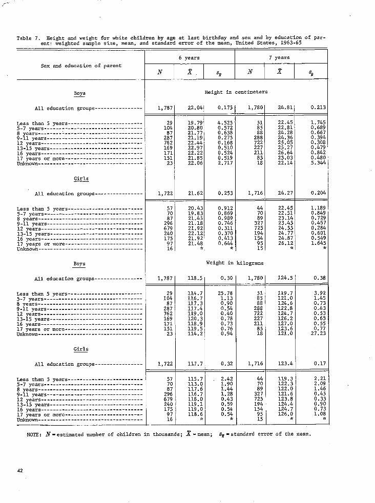
Table 7. Height and weight for white children by age at last birthday and sex and by education of parent: weighted sample size, mean, and standard error of the mean, United States, 1963-65

6 years 7 years Sex and education of parent I I I I

N x. sz N x %


All education groups---------------- 1,787 22.04 0.175 1,780 24.81 0.213

QSS than 5 years-------------------------5-7 years---------------------------------8 years-----------------------------------g-11 years--------------------------------12 years----------------------------------13-15 years-------------------------------16 years----------------------------------17 years 01 more--------------------------Unknown-----------------------------------

19.79 4.525 22.45 1:: 20.80 0.572 2; 22.81

21.77 0.638 24.28 2::: 21.19 0.275 2% 24.36 762 22.44 0.168 722 25.05169 22.97 0.510 227 25.27 171 22.22 0.524 211 26.64 151 21.85 0.519 a5

23 22.06 2.717 18 fE2.

1.745 0.689 0.667 0.394 0.308 0.479

E% 51344

Girls


mess than 5 years------------------------- 57 20.43 0.912 22.455-7 years--------------------------------- 70 19.83 0.869 % 22.51 k% 8 years----------------------------------- 21.45 0.989 23.14 0:729 g-11 years-------------------------------- 2:: 21.18 0.746 3% 23.45 0.45712 years---------------------------------- 679 21.92 0.311 725 0.284 13-15 years------------------------------- 240 22.12 0.370 194 1% 0.60116 years -___-___--__------------------- 175 21.92 0.413 154 24187 17 years or more-------------------------- 21.48 0.644 95 26.12 * !‘E. Unknot----------------------------------- 91: * * 15 j,

Bovs Weight in kilograms

All education groups---------------- 1,787 .18.5 0.30 1,780 124.5 0.38

&ss than 5 years-------------------------5-7 years---------------------------------8 years-----------------------------------

1% 114.7 116.7 117.3

25.78 1.13 0.90

2; 119.7 121.0 124.6

3.92 1.45 0.73

9-11 years--------------------------------1-J years----------------------------------13-15 years-------------------------------16 years----------------------------------17 years or more--------------------------unknown-----------------------------------

2% 762 169 171151

23

117.4 119.0 120.3 118.9 119.5114.2

0.54 0.40 0.78 0.73 0.76 0.94

2:: 722 227 211

E

122.8

E t;127:0 123.6 121.0

0.43 0.53 0.63 0.55 0.77

27.23

Girls


Less than 5 years------------------------- 57 115.7 , 2.42 44 119.3 2.21 5-7 years--------------------------------- 70 113.0 1.90 70 122.3 2.098 years----------------------------------- 117.6 1.44 122.0 1.46 9,;1~,~~~"-------------------------------- 2;: 116.7 1.28 ;;; 121.6 0.45

-___-_____------------------------ 679 118.0 0.43 123.8 0.33 13-15 years------------------------------- 240 119.1 0.59 194 124.4 0.9016 years---------------------------------- 175 119.0 0.54 154 124.7 0.73 17 years or more-------------------------- 118.6 0.54 95 126.0 1.08 Unknown----------------------------------- 9L67 * * 15 * *

NOTE: N-estimated number of children in thousands; x= mean; S%=standard error of the mean.

42

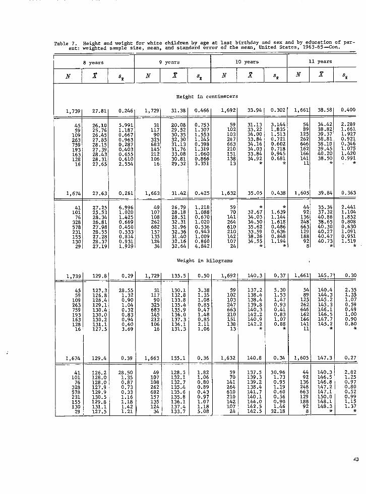
35.34

129

--

Table 7. Height and weight for white children by age at last birthday and sex and by education of parent: weighted sample size, mean, and standard error of the mean, United States, 1963-65-Con.

I 8 years 9 years 10 years 11 years

N x S-x N 1 sx N x ' sp N x sz --~_


1,692 33.94 0.302

45 26.10 20.08 0.753 3.144 2.289 25.76 1.307 15092 $2 1.835 1.661

1:; 26.45 390% 1.553 103 34:oo 1.513 1.927 263 27.85 32:30 1.245 247 33.84 0.721 759 28.15 31.13 663 0.602 Ei

27.39 31.76 ET98 210 %Z 0.718 1:075 2: 28.43 33.08 11060 151 33:84 0.945 1.420 128. 28.31 30.81 0.866 138 34.92

* 0.681

* 0.991

*16 27.65 29.32 3.351 13

1,674 27.63 31.42 0.425 1,632 35.05 0.438 1,605/ 39.84 0.3634= I I - -

1% 27.25 26.79 1.218 59 2.44128.18 1.088 70 32.6; 1.63; $4 37.32 1.104 28.51 0.670 141 34.03 1.144 1.852

3:: fE26:81 32.31 1.020 264 1.618 2: $E 0.80831.96 0.536 610 %; 0.486 663 40130 0.630

578 IE 32.36 0.943 210 33:59 1.0912: 27128 31.40 1.009 142 38.26 F% 188 %E 130 28.37 32.16 0.860 107 34.55*

1:194*

g82 40:73*

::95:;*29 27.19 32.64 4.842 24

Weight in kilograms

1,739 129.8 0.29 1,729 135.5 0.50 1,692 140.3 0.37 1,661 -__

45 127.3 28.55 130.1 3.38 5.30 140.4 2.35 126.8 1.32 1217 132.8 1.35 1:; EZ 1.53 2: 144.3 1.35

1:; 128.4 0.90 133.8 1.08 103 138:4 1.47 125 145.2 1.07 263 129.1 1.04 3% 135.4 0.85 247 139.8 0.93 262 145.3 0.59759 130.4 0.32 683 135.9 0.47 663 140.3 0.41 646 146.1 0.49 193 130.0 0.83 145 136.0 1.48 210 142.2 0.83 162 146.5 1.00 163 0.94 212 137.3 0.85 151 140.9 1.07 166 147.7 0.90

K 0.60 106 136.1 2.11 138 142.2*

0.88*

141 145.2*

0.80% 127:5 3.69 16 131.3 1.06 13 11 6

1,674 129.4 0.39 1,663 135.1 0.36 1,632 140.8 0.34 1,605

126.2 28.50 128.5 1.82 137.5 30.96 140.3 2.821% 128.0 1.35 1% 132.1 1.06 % 1.73 z”; 146.5 1.25

128.0 0.87 108 132.7 0.80 141 E23 0.95 136 146.8 0.973:: 127.9 0.73 262 135.4 0.89 264 13814 1.19 248 147.2 0.80 578 129.9 0.33 682 135.6 0.43 610 141.7 0.60 663 147.1 0.52231 130.5 1.16 157 135.8 0.97 210 140.1 0.56 129 150.0 0.99155 129.8 1.18 135 136.1 1.07 142 144.0 0.90 188 148.1 1.15 130 131.1 1.42 124 137.4 1.18 107 142.5 1.46 92

8 148.3* 1.37*29 127.5 1.21 34 133.7 5.08 24 142.5 32.18

43

------------------------------------

---------------------------------- ----

----------------------------------

---------------------------------- ----------------------------------

--------------------------------

-------- -------- -----

----------------------------------

Table 8. Height and weight for Negro children by age at last birthday,sex,and annual family income:weightedsample size, mean, and standard error of the mean, United States, 1963-65

6 years 7 years Sex and annual family income


*ll incomes------------------------------ 289 119.1 0.72 125.2 0.59

Less than $500--------------------------------- 4 * K $.joo-$ggg-$l,ooo-$l,ggg---------------------------------- 2 119.1

G< 2.0:

;;;.j 5.6;

$2,000-$2,ggg 119.5 2.73 125:9 x$3,000-$3,ggg------- --_---------- --__-----_ s32 118.3 1.16 126.7 2:65$4,000-$4,ggg 120.5 27.03 124.6 0.88$5,000-$6,999---------------------------------- 2: 118.9 1.99 128.0 2.33$7,ooo-$g,ggg---------------------------------- 27 121.7 1.58 125.4 2.21$~0,000~$~4,ggg~~~~~~~~~~~~~~~~~~~~~-~~~~-~-~-~ 5 3< * $15,000 OL‘moTe--------------------------------Don't know------------------------------------- i Gc * 123.; 3.0;No response------------------------------------ 6 * 9

Girls

All incomes------------------------------ 280 118.5 0.86 124.6 0.59

Less j-ha,-, $500---------------------------------$500-$999-------------------------------------- f T 117.: 1.6; 125.; 1.8;$1,000-$1,ggg 47 119.3 0.86 123.5 1.17$2,000-$2,ggg 117.4 1.30 124.4 1.48

3,000-$3,ggg---------------------------------- 2 117.6 2.40 123.9 1.63 $ 4,000-$4,ggg---------------------------------- 33 118.2 2.64 125.2 2.50$5,000-$6,999-m- _______-___ -__- ______ -___- _____ * * 125.5 1.68$7,ooo-$g,ggg---------------------------------- :67 7-c 9< 124.3

Jr 3.49

*$10,000-$14,ggg$15,000 01 mope--------------------------------Don't know-------------------------------------No response------------------------------------ i x t 9,

e * *

Boys Weight in kilograms . *ll incomes------------------------------ 289 21.76 0.37 24.04 0.32

~~~~ than $500--------------------------------- 4 * f $5orJ-$ggg- _-___________--_ k 23.39 2.9;$l,ooo-$l,ggg---------------------------------- 51: 21.9; 1.04 23.24 1.07$2,000-$2,ggg __________--________-------------- 21.43 1.87 24.71 0.94$3,000-$3,ggg---------------------------------- 832 20.95 23.51 1.02$4,000-$4,ggg---------------------------------- 23.88 E 24.34 0.89$5,00,-J-$6,999 ____________________-------------- 5; 20.69 0173 24.61 1.16

7 ooo-$g,ggg---------------------------------- 25.00 1.55 24.42 1.45 s 1~,000-$14,ggg-------------------------------- 5 * 7-c $15,000 or moTe--------------------------------Don't know------------------------------------- i 9i * 24.66 1.70No response------------------------------------ 6 9, *

Girls

All incomes------------------------------ 280 21.09 0.36 23.69 0.47

mess than $500--------------------------------- 18$.jo()-$ggg ___- ____________-_____-_-------------- 20.4; 0.6; 24.13 0.89

2: 21.69 0.76 23.50~:~~~~1$'2y~~~:::III~~~~~~~~~~~~~~~~~~~~~~~~~~~~ 0.95 23.97 c:;$3~000-$3~ggg 2 IFI% 1.35 21.98 0:66 $4,000-$4,ggg ___-_----_--_--------------------- 21:04 1.27 24.69 1.12 $5,OOO-$fj,999 __________________-_-------------- 263 t * 24.01

7,ooo-$g,gg9---------------------------------- 17 * <c 24.69*

'f*92 $ 10,000-$14,g99-------------------------------- * * $15,000 01 moTe--------------------------------Don't know------------------------------------- i * 4 4 * No response------------------------------------ * *

NOTE: N=estimated number of children in thousands; x = mean ; sx=standard error of the mean.

Table 8. Height and weight for Negro children by age at last birthday,sex,and annual family income:weightedsample size, mean, and standard error of the mean, United States, 1963-65-Con.

8 years 9 years 10 years 11 years


279 131.3 0.57 268 135.0 0.67 264 139.6 0.97 145.7 0.50

* * * * * * 133.3 3.6; * 146.; 3.70

131.1 ;.gH 132.2 2.34 137.5 1.5: 145.1 0.89 131.3 134.7 3.22 139.4 2.30 144.0 4.75 130.5 0:94 135.4 2.61 136.7 1.60 143.4 2.50 131.1 144.8 3.40 150.3 1.90 131.5

* E! 135.; 1.4: 140.3 31.62 3.11

* 136.9 2.32 143.8*

4.40*

Xi 3.45* *

* * 16 138.2*

31.09* * * * *

3

280 129.4 0.52 265 137.5 0.90 265 141.8 0.65 149.2 0.69

4; 126.; 31.0;50 130.1 2.42

1.36 i?; %-'; 3.62 58 129:1 1.44 11 132.7

* 3.60

*4

18 126.; *

4.60*6

279 27.50 0.42

*

;;A$

25:93 26.8727.81

* *

*

280 26.95 0.37

445 23.9; 0.6;

1.71 203 % % 1.77

30:21 5187 26.10 x 11 28.91

* 1:92

*4

18 28.3; *

3.5j6

L

4 136.: 3.6; 142.; 2.9; 148.: 33.4: 138.4 2.62 $3 139.8 2.62 148.3 1.60 135.6 2.09 64 142.8 2.21 151.7 1.34

1.47 32 137.8 5.08 149.4 1.88 z-z 3.42 12 144.3 146.7 2.27 135:5 1.86 142.9

* ";*E 149.7 1.85

144.4 3.80 :99 - * 149.8 33.59

* * * * 148.; 2.3;* * * * ,

Weight in kilograms

29.45 0.77 264 32.43 0.72 36.78 0.50

t * * 28.3; 2.27

%X x 29:21 1:98

30.5: 1.4;30.00 2.45

31.3:

E;38:17 33.07 33.4;

1.0: 1.870.92 3.02 7.86 3.27-R

35.6;35.9836.78 34.0239.60 37.9435.43

1.861.89 2.85 1.562.542.12 3.52

29.32 7.2; * x * * x

31.17 0.62 265 35.67 0.89 41.11 1.45

4 * * 29.8: 2.6: 36.1; 3.1:

2 33.31 2.04 41.8; ;.;;29.9; 1.2: 64 36.64 2.27

1.46 32 32.88 2.00 Ki 3:53 "3% 2.38 12 37:12 2.03 30:91 1.80 37.3; 3.22*

41.42 2.52 40.60 1.76 1: * 42.92 10.26

* * 9 * *

* *

1;6

37.4;*

3.39P3

45

Table 9. Height and weight for Negro children by age at last birthday and sex and by education of parent: weighted sample size, mean, and standard error of the mean, United States, 1963-65


= Height in centimeters

All education groups---------------- 285 119.1 0.72 286 125.2 0.55

Less than 5 years------------------------- 17 117.4 0.40 22 125.5 0.32 5-7 yea*s--------------------------------- 2s 9s t 35 124.1 3.u g yea*s----------------------------------- 23 119.6 2.69 16 ;v d g-11 yea*s-------------------------------- 82 118.1 1.73 77 124.7 0.75 12 years---------------------------------- 105 119.7 0.74 102 126.7 0.9t 13-15 years------------,------------------- 18 122.0 2.24 6 7-r ?! 16 years---------------------------------- 8 * * 7 * d 17 years or *ore--------------------------Unknown----------------------------------- 1 Y 18 * d

Girls


Less than 5 years------------------------- 14 * t4

5-7 years---------------------------,------ 47 118.3 2.07 42 123.3 0.93 g years----------------------------------- 44 115.2 1.50 34 123.2 1.15 g-11 years-------------------------------- 89 118.5 1.21 70 123.0 1.50 12 years---------------------------,,------- 62 120.7 1.63 80 126.2 0.98 13-15 years-------------------------------16 years------------------------------,----

18 4

120.7 1.45 20 X * 8

128.5 *

0.73 d

17 years or more---------------------,---, 7 * * Unknown----------------------------------- 13 * w 6 * *


All education groups---------------- 289 286===I== 24.04 0.32

Less than 5 years------------------,___ 17 21.16 2.71 22 24.75 1.53 5-7 years--------------------------------- 29 * * 35 23.91 1.28 8 years---------------.---.---,___________ 23 21.70 5.07 16 * * 9-11 years----------------------,,__,___ 82 21.70 0.86 77 23.70 0.85 12 years------------------------_-__,_____ 105 21.44 0.57 102 24.32 0.43 13-15 years----------------------________ 16 years------------- ---------__---_-_____

18 8

24.90 2.21 6 * * 7

* *

* *

17 years or mo*e--------------------------Unknown-----------------------__________-- 4 * * 18 * *

Girls


Less than 5 years------------------------- -I - 14 * * 5-7 years--------------------------------- 47 20.21 0.85 42 22.83 0.69 g years----------------------------------- 44 19.79 0.73 34 23.61 1.09 9-11 years-------------------------------- 89 21.11 0.45 70 23.19 0.9912 years--------------------------------,- 62 22.41 0.88 80 23.60 0.63 13-15 years------------------------------- 18 22.01 0.6: 20 26.67 1.0716 years--------------------------------,, 4 * 9 8 * 9 17 years ,J* more-------------------------- 7 * Ji "*known----------------------------------- 13 * * 6 * d

NOTE: N -estimated number of children in thousands; x=mean; SF= standard error of the mean.46

Table 9. Height and weight for Negro children by age at last birthday and sex and by education of parent: weighted sample size, mean, and standard error of the mean, United States, 1963-65-&n.

I I I a years 9 years 10 years 11 years

N x 8% N 1 sz N x -3 N Jr 352


279 131.3 0.57 268 135.0 0.67 254 145.7 0.50

8 * * 19 138.1 1.38 * 14 * * 54 130.1 1.26 68 133.1 2.09 3.45 47 143.7 4.40 29 131.3 3.15 22 136.3 3.15 2.59 33 145.2 1.88 87 131.0 0.82 70 134.1 1.25 2.00 74 144.6 1.37 71 131.2 1.56 63 135.5 1.83 1.23 64 148.3 1.83 20 134.5 2.57 15 135.4 5.31 11 * * 2 * *

3 * * 4 * * 14 * * 2 * * 3 * * 3 * *

4 * * 10 * * 13 * *

*

280 129.4 0.52 265 137.5 0.90 265 141.8 0.65 252 149.2 0.69

6 * * 15 * * 11 * * 18 150.1 3.36 47 130.4 2.64 20 137.7 6.27 50 142.1 2.13 44 151.0 1.63 23 125.9 1.70 38 136.7 3.32 21 142.7 3.97 37 148.6 1.16 75 128.1 0.75 66 136.0 2.16 101 144.0 1.85 73 149.4 1.51 71 131.4 0.99 84 138.3 2.14 55 139.5 3.87 62 147.6 1.31 17 128.2 2.33 11 * * 14 .s * 6 * * 13 131.6 2.94 7 * t

1 * * 2 * * 10 * x 23 128.0 3.36 17 137.9 3.72 9 * *

Weight il I kilograms

279 27.50 0.42 268 29.45 0.77 264 32.43 0.72 254 36.78 0.50

8 1 * 19 30.02 1.69 8 x * 14 * * 54 26.96 0.67 68 28.97 1.57 36 34.32 3.03 47 38.79 3.11 29 28.82 2.91 22 30.99 3.14 28 32.31 2.42 33 35.76 1.50 67 27.22 0.76 70 27.73 0.89 83 32.33 1.00 74 34.45 0.96 71 26.61 0.83 63 29.13 0.80 70 31.60 1.06 64 39.06 1.76 20 30.28 1.93 15 33.59 6.03 11 * * 2 * *

3 * * 4 * * 14 * * * * 3 * * * *

4 * * 10 * * , *

*

280 26.95 0.37 265 31.17 0.62 265 35.67 0.89 252 1.45

6 * * 15 * * 11 * * 18 9.95 47 26.78 1.25 20 31.34 5.29 50 35.07 1.41 44 1.91 23 23.86 1.10 38 29.18 1.22 21 35.38 2.95 37 1.88 75 26.70 0.83 66 29.86 1.74 101 36.13 1.79 73 3.84 71 27.69 1.10 84 31.56 1.63 55 34.49 2.03 62 1.21 17 27.48 2.61 11 * * 14 * * 6 x 13 28.14 6.59 7 * *

1 * * 2 * * 10 * * 23 28.01 1.24 17 29.63 2.12 9 *

- -

41.11

41.17 42.65 37.40 44.22 38.07

*

47

w

Table 10. Use of the sign test and z-test to compare the mean height and weight of childE;ztzi extreme family income and education groups, by age of child at last birthday and sex: States, 1963-65

Annual family income Education of parent

Age and sex Less than $15,000 or Less than 17 years$500 more Sign z- 5 years or more Sign Z-

test1 test' test1 test'

x sz x sn B sn x s2

Boys Height in ce ntime te rs

6 years-----7 years-----8 years-----9 years-----10 years----11 years----

1.12 119.6E% 1.82 126.7 2.15 130.3 2.35 138.2 2.82 140.7

2.06 146.9

0.86 1.03 1.29 1.14 1.14 0.78

-3.12 115.7 2.68 -1.77 121.5 2.82

0.27 128.3 133.1 f-2

I;*:; 137.0 3:63 -Loo 142.1 1.89

119.5 123.6 130.7 136.1 142.0 145.3

0.76

tz 2:11 0.86 0.76

-1.36 -0.72 -0.99 -0.97 -1.34 -1.57

Girls

6 years-----7 years-----8 years-----9 years-----10 years----11 years----

116.7 1.56 118.5 121.4 2.88 126.7 126.3 1.70 130.8 135.0 3.91 138.6

2.00 143.2 A 2.17 145.5

0.77 0.70 1.56 1.64 1.18 2.12

-1.03 115.7 2.42 -1.79 121.1 2.99 -1.95 126.1 3.01 -0.85 130.7 1.54 -1.03 136.3 3.76 -0.43 143.2 2.54

118.6 125.8 131.3 137.7 142.5 148.6

0.54 1.03 1.43 1.27 1.29 1.43

-1.17 -1.49 -1.56

t-3.51 -1.56 -1.85


6 years----- 22.08 0.484 -2.34 20.30 1.623 21.85 0.519 -0.91 7 years----- 26.73 1.193 -2.51 1.136 23.03 0.480 + 0.09 8 years----- !!I#!!?28.04 0.925 -0.10 2 52 1.840 28.07 0.651 -0.66 9 years----- 1:329 2.157 28:20 1.114 0.866 -1.85 10 years---- 29.41 2.275 E% 0.767 1'1, ;; 30.75 2.343 Et 0.660 -1.68 11 years---- -36 90 1.806 39: 20 1.003 -1:11 34.84 1.567 38:41 0.986 -1.93

Girls

6 years----- 20.34 0.469 22.35 0.963 -1.88 20.43 0.912 21.48 0.644 -0.94 7 years----- 22.40 0.979 25.65 0.655 -2.76 22.60 1.038 26.49 1.628 t-2.02 8 years----- 26.06 1.393 27.89 1.444 -0.91 26.86 2.721 28.46 0.928 -0.56 9 years----- 27.31 32.20 1.342 -1.52 28.76 1.527 32.31 0.810 t-2.05 10 years---- E 36.88 1.094 32.62 2.859 34.30 1.046 -0.55 11 years---- % % 3.290 40.19 1.635 I;*;;. 37.06 1.400 40.73 1.455 -1.82A -

'See discussion of "Test for.consistency of a relationship' in appendix I. ?See diy:;tzio;of "z-test" in append= I. NOTES: +=standard error of the mean. Underscoring denotes a pooled value necessitated by unreliable estimates computed from smaller

fy4&gs (see "Standards of reliability and precision" in appendix I). In the columns of

for income than $500 a year, the pooled means and standard errors represent incomes less than

$1,000 a year,and in the columns for income of $15,000 or more a year,the pooled values representincomes of $10,000 or more.

49

-----------

------------

------------

-----------

Table 11. Summary of Daniel's Test for Trend1 and weighted least squares' slopes for relationshipof height and weight to annual family income,for children by age at last birthday, sex,and'race: United States, 1963-65

Height in cm. vs. annual Weight in kg. vs. annual family income family income

Age, sex, and race -

Spearman's Slope Spearman's SlopeZdi* rs b z Zdi* r s b

TOTAL

Boys

6 years----------- to.8167 0.031 0.007 t4.55 0.023 0.005 t4.887 years------------ to.8833 0.018 0.007 t2.37 0.017 0.006 t3.01 8 years------------ -0.0788 0.009 1.72 0.012 0.007 1.63 9 years------------ to,8303 :*:31: 0.011 t2.96 0.022 0.007 t3.02 10 years----------- to.1091 01026 0.008 0.025 0.008 13.17 11 year- to.6833 0.011 0.010 'X . 0.018 0.011 1.63

Girls 6 years-----------.. to.5757 0.025 0.008 t3.18 to.7878 0.020 0.006 t3.37 7 years --_---^----- to.9394 0.024 0.008 t2.99 to;9030 0.026 0.006 t4.33 8 year------------- to.8667 0.028 t3.56 TO.7667 0.021 0.008 'f2.80 g years------------ to.7575 EE t3.11 0.040 0.009 t4.45 10 year------------ to.7167 KE 0:oos t4.11 :;*g; 0.016 0.009 1.81 11 years----------- 0.3833 0:02a 0.010 T2.81 0:2167 0.018 0.016 1.17

WHITE

Boys

6 year------------- t0.8000 0.037 0.007 t5.35 TO.8500 0.025 0.005 t5.307 years to.8666 0.017 0.008 t2.13 to.8166 0.012 0.006 1.898 years-----------. 0.3697 0.019 0.009 t2.22 1.609 years------------ to.8500 0,027 0.012 t2.37 :oo*gg ES E% t2.3810 years----------- to.6606 0,024 0.009 t2.64 TO:6969 0:019 0:oos t2.1711 year------..----- t l.OOOO 0.015 0.013 1.19 0.5666 0.010 0.012 0.81 Girls

6 years------------ to.6500 0.031 0.009 t3.56 0.5666 0.026 O.OQ6 t4.027 years------------ to.8909 0.037 0.009 t4.28 to.9272 0.032 0.006 t5.358 years------------ TO.7666 0.030 0.009 t3.47 0.020 0.008 t2.309 years----------..- TO.8666 0.029 0.009 t3.36 $8';;; 0.043 0.010 t4.3010 years----------- to.9333 0.044 0.010 t4.54 to: 7000 0.021 0.010 t2.0011 years----------- 0.5166 0.038 0.011 t3.63 0.4500 0.029 0.016 1.84 NEGRO

Boys 6 years-- _____-____ 0.6071 0.047 0.029 1.61 0.3214 0.016 0.020 0.82 7 years------------ 0.6071 0.014 0.033 0.43 0.5714 0.013 0.63 ; ;~~Es~------------ -0.4643 .O.Oll 0.036 -0.30 so.013 Ef;

to.9429 0,050 0.037 1.34 0.027 0:034 -;A;

10 years----------- 0,3929 0.08a 0.059 1.48 0.030 0.041 0173 11 years----------- -0.2143 0.028 0.038 0.74 0.023 0.038 0.61

Girls 6 years------------ 0.3714 0.001 0.069 0.02 0.4286 0.010 0.0317 years------------ 0.2071 0.014 0.013 1.11 -0.1786 0.009 0.0178 years------------ 0.6000 0.065 1.87 0.054 0.0209 years------------ 0.1429 0.065 E% 1.30 EE 0.144 0.03010 years 0.032 01059 0.53 0:3000 0,021 0.066

.11 years----------- -E'L:: ,O.Oll 0.060 -0.19 -0-4643 0.034 0.080

'See discussion on "Test for Trend" in appendix I. 2See discussion on "Weighted least squares as a test for trend" in appendix I. *Significant at .05.

50

----

------------

Table 12. Summary of Daniel's Test for Trend* and weighted least squares? slopes for relationshipof height and weight to education of parent, for children by age at last birthday,sex,and race: United States, 1963-65

-

T Height in cm. vs. annual Weight in kg. vs. annual family income family income

Age, sex, and race Slope

Zdi* Spearman's Slope z Zdi ”

Spearman's Tb5 b =.

TOTAT,

Boys

6 years------------ to.8571 0.280 0.090 t3.12 to.7619 0.215 0.055 t3.897 years------------ 0.6190 0.495 0.084 t5.86 0.3095 0.263 0.068 t3.88 g years------------ to.9285 0.104 t2.15 to. 8809 0.146 0.069 t2.119 years------------ E95 0.107 +3.t33 to:7381 0.090 t3.6710 years----------- :;.;;;: 0: 388 0.120 +3.23 to.8095 if 2;; 0.113 1.0611 years----------- to: 8333 0.355 0.106 t3.34 0.4523 0:267 0.119 t2.24

Girls

6 years -_----- - to. 8809 0.326 0.094 t3.47 +'0.7619 0.175 0.050 t3.527 years------------ 0.368 0.110 t3.35 to.9047 0.229 q.059 t3.908 years :;* g;: 0.347 0.110 t3.15 0.191 0.085 t2.269 years------------ +O: 9226 0.424 0.094 t4.51 :;- ;g;; 0.412 0.089 t4.6110 years----------- to. 7857 0.240 0.109 t2.20 to: 7381 0.292 0.106 +'2.7711 years----------- +O. 7619 0.204 0.112 1.81 to.9047 0.222 0.100 t2.21

WHITE

Boys

6 years------------ to. 8809 0.328 0.105 t3.13 to.7619 0.225 0.065 +3.487 years------------ to. 7142 0.526 0.087 t6.02 0.6428 0.293 0.074 t3.978 years------------ to.9047 0.304 0.123 +2.4t? to. 8809 0.153 0.086 1.779 years------------ t0.9762 0.451 0.124 +3.65 +O. 6904 0.413 0.076 t5.4710 years----------- to.9285 0.384 0.143 t2.69 +0.7142 0.069 0.130 0.5311 years----------- to.7619 0.383 0.114 t3.36 0.4762 0.216 0.144 1.49

Girls

6 years------------ 0.345 0.106 t3.25 0.142 0.058 '2.467 years------------ 0.464 0.111 t4.19 :;- ;g; 0.236 0.068 t3.45 g years------------ 0.348 0.134 +2.59 0:6190 0.205 0.106 1.949 years------------ 0.533 0.103 t5.17 +O. 6904 0.474 0.089 t5.3210 years----------- 0.342 0.123 t2.78 to. 7500 0.279 0.129 t2.1611 years----------- 0.352 0.123 t2.86 0.6190 0.349 0.120 t2.92

NEGRO

6 years------------ 0.248 0.080 t3.11 0.7000 0.146 0.249 0.597 years------------ :-E l 0.009 0.080 0.11 0.4000 0.000 0.143 -0.008 years------------ 0:7000 0.340 0.275 1.24 0.1000 0.085 0.162 -0.589 years------------ -0.0286 0.334 0.194 -1.72 0.2571 0.009 0.176 -0.5010 years----------- 0.7000 0.076 0.492 0.15 0.1000 0.114 0.405 -0.2811 years----------- -0.2000 0.300 0.127 -2.37 0.2000 0.035 0.279 -0.13

Girls

6 years------------ 0.8000 0.620 0.259 t2.39 0.8000 0.299 0.116 t2.58 7 years------------ 0.0857 0.583 0.126 t4.62 0.7714 0.220 0.105 t2.10 8 years -_-___-_____ 0.5429 0.504 0.223 t2.26 +0.%357 0.318 0.172 1.85 9 years------------ 0.6000 0.590 1.02 0.4000 0.566 0.413 1.37 10 years----------- -0.1000 0.120 EE 0.20 0.4000 0.036 0.394 0.09 11 years----------- -0.8000 0.405 0:331 -1.22 -0.1000 0.474 0.358 -1.32

'See discussion on "Test for Trend" in appendix I.. 2See discussion on "Weighted least squares as a test for trend" in appendix I. 3Sum rounded to nearest whole unit due to tie in ranks.

.tSignificant at .05.

51

cutoff

Table 13. Percent of children falling below the lowest 10th United States,

heights and weightsspecific to each age-sex group, by annual family income:

percentile of 1963-65

l II Annual family income

Age' and sex percentilelath iAL /


6 years-------------------------------------- 111.8 10.1 *

7 years-------------------------------------- 117.8 9.4 *

8 years-------------------------------------- .123.3 10.0 *

9 years-------------------------------------- 127.0 9.4 *

10 years------------------------------------- 131.4 10.6 *

11 years------------------------------------- 137.2 10.6 *

Girls

6 years-------------------------------------- 110.6 8.8 *

7 years-------------------------------------- 116.3 10.2 *

8 years-------------------------------------- 121.4 9.7 *

9 years-------------------------------------- 127.1 10.4 Jr

10 years------------------------------------- 132.0 10.7 Jr

11 years------------------------------------- 138.9 10.3 *

Boys Weight in ki .ograms

6 years-------------------------------------- 18.15 10.2 Jr

7 years----'---------------------------------- 20.38 8.0 *

8 years-------------------------------------- 22.62 8.7 *

9 years-------------------------------------- 24.46 8.7 Jr

10 years -___________-------_----------------- 26.70 9.9 9c

11 years------------------------------------- 30.05 9.1 *

Girls

6 years-------------------------------------- 17.56 8.6 *

7 years-------------------------------------- 19.52 11.1 *

8 years-------------------------------------- 21.66 9.8 *

9 years------------------------------------,-- 24.34 9.3 *

10 years------------------------------------- 26.18 9.9 *

11 years------------------------------------- 29.83 9.8 Jr

'Denotes age of child at last birthday; it is not the mean age for the group. text for discussion.

39.5 19.1 15.7 22.2 10.6 16.2 22.1 19.6

* 27.9 11.4 10.5

0.0 20.4 11.2 16.6 27.4 14.0 12.8 19.1

8.5 19.3 11.8 16.1

34.6 7.0 15.7 21.7

7.9 7.8 17.5 19.9

7k 24.0 5.2 12.0

0.0 13.7 8.8 24.4

20.6 21.0 4.7 15.4

13.0 15.5 39.0 11.9

See page 5 of

52 .

Table 13. Percent of children falling below the lowest 10th percentile of heights and weightsspecific to each age-sex group, by annual family income: United States, 1963-65-Con.

Annual family income-Con.

$7,000- $10,000- $15,000$9,999 $14,999 or more


7.3 9.0 17.2 6.6 8.1 5.5 0.0 20.8 6.6 6.3 8.0 8.3 4.1 2.2 22.9 13.7 10.7 10.8 3.8 3.8 5.6 13.6 22.2 4.2 8.2 6.4 3.7 7.1 17.1 20.0 7.7 9.2 5.6 7.9 4.1

8.4 18.9 15.3 8.3 9.8 8.3 7.1

16.9 9.5 9.6 7.4 6.2 3.3 3.8 3.9 22.1 6.1 12.2 6.5 7.6 0.0 9.9 16.6 10.8 9.9 7.0 0.9 8.1

11.1 16.3 11.5 7.2 9.6 8.6 0.0 15.8 16.5 13.1 9.7 8.8 3.8 0.0 12.1 8.9 14.5 12.8 6.6 0.0 12.1

Weight in kilograms

15.3 7.8 13.5 9.5 7.0 10.0 0.0 11.2 6.9 11.2 8.2 5.4 2.7 0.0 22.3 11.9 11.0 7.9 5.0 5.3 3.2 20.8 14.3 10.6 7.2 5.4 2.7 0.0 12.5 18.5 7.3 8.5 7.0 4.0 3.5

5.5 17.0 4.7 12.6 6.5 9.8 2.3

15.2 18.9 8.2 8.6 5.6 3.2 3.6 3.7 26.6 8.3 10.5 7.4 9.6 0.0

12.8 21.6 14.1 7.8 4.7 0.9 8.1 15.8 17.3 9.7 6.2 7.1 8.1 0.0 19.2 6.7 8.4 6.2 9.2 10.9 3.2 11.3 8.2 15.7 7.0 8.8 1.6 3.6

53

------------

---------

------------

-----------

-----------

.Table 14. Percent of children falling below the lowest 10th percentile of heights and weights specific to each age-sex group, by education of parent: United States,1963-65

Education of parent

Age1 and sex 17 16 years

years or more


6 years------------ 111.8 39.7 14.8 6.3 16.1 7.7 3.4 9.5 4.5 7 years------------ 117.8 43.4 26.1 0.0 13.3 9.1 3.3 1.4 7.1 8 years------------ 123.3 15.6 10.8 9.3 16.0 7.9 13.4 9'. 5 0.0 g years 127.0 27.8 21.5 12.4 11.9 7.0 14.1 3.2 11.3 10 years-- 131.4 23.6 21.8 21.9 12.1 10.2 1.8 3.1 4.8 11 years----------- 137.2 23.7 17.1 10.9 12.9 9.6 6.1 5.8 8.9

Girls

(j years------------ 110.6 21.4 17.4 13.9 14.8 9.1 2.0 3.5 0.0 7 years------------ 116.3 13.0 15.9 14.7 11.5 9.2 3.8 6.i 7.5 g years 121,4 27.8 6.4 19.1 12.2 7.8 6.4 12.c 8.2 9 years------------ 127.1 30.0 28.5 12.4 7.4 6.5 9.9 11.8 3 ..5 10 years 132.0 18.9 12.5 8.2 15.9 9.2 11.2 3.4 4.0 11 years----------- 138.9 30.0 10.1 11.2 11.6 10.4 4.6 4.i 5.6


6 years _______-_--- 18.15 16.4 8.9 6.3 1 13.7 I 8 .: 4.6 , 9.4 10.1 7 years------------ 20.38 24.7 25.0 -2.3 1 9.8 , 5.i 9.1 1.4 7.8 8 years------------ 22.62 6.5 11.6 13.5 14.2 7.1 12.8 7.2 0.0 g years------------ 24.46 15.7 21.6 19.7 8.8 7.3 10.2 2.9 0.0 10 year------------ 26.70 23.2 18.3 20.4 11.0 9.5 2.7 2.2 6.1 11 year------------ 30.05 20.2 9.3 15.4 13.9 7.8 8.6 9.0 3.5

Girls

6 years ____________ 17.56 14.7 14.8 15.0 14.6 7.9 3.1 7.6 0.0 7 years------------ 19.52 13.0 14.9 16.9 17.5 8.8 6.1 5.0 3.2 8 years- 21.66 11.7 19.1 22.4 15.1 7.6 6.0 2.7 8.2 9 years------------ 24.34 23.4 29.4 7.8 10.8 7.7 5.2 6.6 4.1 10 years -_---- ---_- 26.18 4.3 15.8 6.2 11.9 8.0 16.5 0.0 10.5 11 years----------- 29.83 46.4 9.2 14.1 14.3 5.9 2.4 7.3 9.5

-

IDenotes age of child at la St birthday; it is not t :he me:ar1 age for the ! Egroup. See pageof text for discussion.

54

Table 15. Summary of Daniel's Test for Trend' for percent of children falling below the lowest within10th percentile

1963-65-each age-sex category for annual family income and education of parent:United States,

Agesand sex

Boys

6 years---------------

, years----------------

8 years---------------

g years----------------

10 years-------------

11 years-------------

Girls

6 years---------------, years----------------8 years---------------g years----------------10 years--------------

11 years-----------

l- Annual family income Education of parent

Height of Weight of Height in

of cm. l-Weight

in of

kg.children in cm. :hildren in kg. :hildren C hildren

.

Zdi* Spearman's Spearman's Spearman's Spearman's

's Sdi* rs Edi* rs rs

18 +0.85 52 0.57 28 to.67 68 0.19 24 + 0.80 12 + 0.90 36 0.57 34 0.60 40 + 0.67 52 0.57 40 0.52 64 0.24 34 + 0.72 14 to.88 20 + 0.76 12 to.86 56 0.53 6 + 0.95 10 + 0.88 8 to.90 36 + 0.70 105 0.13 8 + 0.90 14 to.83

46 + 0.62 84 0.30 4 + 0.95 10 to.88 66 0.45 96 0.20 14 +0.83 20 to.76 22 + 0.82 30 to.75 58 0.31 26 +0.69 20 + 0.83 51 0.58 18 + 0.79 6 to.93 22 + 0.82 42 to.65 20 + 0.76 88 0.05 44 + 0.63 22 +0.82 22 + 0.74 38 0.55

ISee discussion on "Test for Trend" it not the mean age for the group. See page 5 of2Denotes age of child at last birthday;

in appendixis

I.

text for discussion. +Significant at .05.

55

---?nti.le

----

Table 16. Percent falling below the lowest 10th percentil.e value for height and weight for each age-sex group of children by, four possible family income dichotomies, and the ratio of above tobeLow within each dichotomy: United States, 1963-65

$2,00@ dichotomy

All10th incomesAge' and sex Pbl.l;Slz;uLOff under Less than I' &?,OOO or^__A

cutoff $2,000, 9'more, per-PFer;e;t cc'~$~~er

I cutoff


6 years---------------------------- 111.8 10.1 25.9 8.2 7 yeara------------------------ 117.8 9.4 20.5 8.1 8 year5. c"""""""""""""""""""-""-"""" 123.3 10.0 13.5 9.5 9 yarns"""""""""""""""""""""""""""" 10 y~~~~""-""-"-"""""-"------------11 years-------------------------

Girls

6 years---------------------------"

7 years""""""""""""""""""""""""""""

8 years----------------------------

9 years--------------------------10 years---------------------------11 years--------------------------

Boys

6 years---------------------------'

7 years------------------"--------

8 years"""""""""""""-"""""""""""""" 9 years""""""""""""""""""""""""""""

10 years-------------------------

11 years---------------------------

Girlq,

6 years----------------------"----

7 years""""""""""""""""""""""""""""

8 years----------------------------

9 years----------------------"----

10 years------------------------------

11 years-------------------------

127.0 9.4 18.6 8.3 131.4 10.6 21.4 9.4 137.2 10.6 12.3 10.4

l.10.6 8.8 15.0 7.9 116.3 10.2 14.7 9.6 121.4 9.7 20.4 8.6 127.1 10.4 16.9 9.4 132.0 10.7 16.8 9.6 138.9 10.3 17.5 9.4

Weight in kilograms

18.15 10.2 17.4 9.3 20.38 8.0 18.4 6.8 22.62 8.7 7.6 8.9 24.46 8.7 17.3 7.6 26.70 9.9 23.3 '8.3 30.05 9.1 9.9 9.1

17.56 8.6 8.8 '8.6 19.52 11.1 *,17.3 10.3 21.66 9.8 20.4 8.7 24.34 9.3, ' 12.1 '8.9 26.18 9.9 '14.8 9.1 29.83 9.8 25.0 7.9

Ratio ofless than $2,000 to $2,000 or

more

3.16 2.53 1.42 2.24 2.28 1.18

1.90 1.53 2.37 1.80 1.75 L.86

1.87 2.71 0.85

i c 2;28

2.8,1 1.09

1.02 1.6'8 2.34 1.36 1.63 3.16

'See discussion on "Test for2Denotes'age of child at last

best possible dichotomy"birthday; it is not the

in appendixfor

I. text for discussion.

mean age the group. See page 5 of,

.

Table 16. percent falling below the lowest 10th percentile value for height and weight for each age-sex group of children byI four possible family income dichotomies, and the ratio of above to below within each dichotomy: United States, 1963-65-Con.

$3,000 dichotomy $4,000 dichotomy $5,000 dichotomy

Less $3,000 Ratio of Less than $4,000 or Ratio of Less than $5,000 or Ratio ofthan $3,000, or more, less than $4,000, more, less than $5,000, more, less than p;e$set

pgere';t $5,000 to $5,000 or

cutoff cutoff .more cutoff cutoff more cutoff cutoff more


18.8 8.2 2.29 15.2 8.1 1.88 15.8 6.2 2.55 20.6 6.8 3.03 16.3 6.8 2.40 13.9 6.9 2.01 18.1 7.8 2.32 16.8 7.1 2.37 15.4 6.6 2.33 16.9 7.9 2.14 18.7 6.3 2.97 14.9 6.6 2.26 19.6 8.6 2.28 19.7 7.3 2.70 16.5 7.2 2.29 10.6 10.6 1.00 13.5 9.6 1.41 14.0 8.7 1.61

15.8 6.7 2.36 14.0 6.4 2.19 13.1 5.9 2.22 10.8 10.1 1.07 14.7 8.4 1.75 12.3 8.8 1.40 15.7 8.5 1.85 16.0 7.3 2.19 14.8 6.8 2.18 14.5 9.2 1.58 15.0 8.4 1.79 14.1 7.8 1.81 16.4 8.9 1.84 16.4 8.0 2.05 15.7 7.3 2.15 15.3 9.2 1.66 13.1 9.2 1.42 13.5 8.4 1.61

Weight in kilograms

16.6 8.8 1.89 13.3 9.0 1.48 13.4 8.0 1.68 15.1 6.3 2.40 12.6 6.3 2.00 12.3 5.6 2.20 14.7 7.2 2.04 13.9 6.6 2.11 13.2 5.9 2.24 18.5 6.7 2.76 17.1 5.8 2.95 15.3 5.1 3.00 18.7 7.9 2.37 18.7 6.7 2.79 15.7 6.6 2.38

7.9 9.4 0.84 11.2 8.4 1.33 9.3 9.0 1.03

11.6 7.8 1.49 13.7 6.4 2.14 12.5 6.1 2.05 12.4 10.9 1.14 17.3 8.6 2.01 14.8 8.7 1.70 17.0 8.3 2.05 18.8 6.3 2.98 17.7 5.2 3.40 13.6 8.1 1.68 14.6 7.0 2.09 13.4 6.5 2.06 16.5 7.8 2.12 14.1 8.0 1.76 12.9 7.9 1.63 19.4 7.6 2.55 15.6 7.6 2.05 15.6 6.3 2.48

-

57 '

Table 17. Height for children by age at last birthday and sex and by education of parentzweightedsample size, mean, and standard error of the mean, United States, 1963-65- -

6 years T 7 yearsTSex and education of parent

N x N

Boys

All education groups---------------- 487 119.5 0.34 494

Less than 5 years------------------------- 2 +I *

5-7 years--------------------------------' 11 9< Jr 5 8 years----------------------------------- 18 119.0 2.45 9-11 years-------------------------------- 109 118.7 0.88 12 years---------------------------------- 246 119.4 0.50 13-15 years------------------------------- 40 121.5 1.68 16 years---------------------------------- 43 120.3 1.51 17 years or more-------------------------- 7 * * unknown----------------------------------- 6 J< *

Girls

All education groups---------------- 427 117.5 0.46 c

Less than 5 years------------------------- 3 * i’

17 99

269 62 30

6 3

487

x ,%

124.5 0.47

119.1 5.10 124.7 28.03 122.8 0.90 124.6 0.69 126.6 1.63 125.5 1.14

* * * *

123.01 0.29

* * 119.4 26.77 119.3 0.81 121.5 0.73 123.3 0.58 125.3 1.32 123.5 1.38

* * * *

r 3 5-7 years--------------------------------- 8 9< * 16 8 years----------------------------------- 3 * * 14 9-11 years -3_------------------------- ---- 63 117.7 1.22 113 12 years---------------------------------- 234 117.1 0.61 240 13-15 years------------------------------- 73 118.5 1.58 62 16 years---------------------------------- 28 116.9 0.97 23 17 years or more-------------------------- 7 * f 2 unknown----- ______________________________ 3 d * 9

NOTE: N=estimated number of children standard error of the mean.

in thousands; 8=mean height in centimeters;~~ =

Table 17. Height for children by age at last birthday and sex and by education of parenkweightedsample size, mean, and standard error-of the mean, United States, 1963-65-Con.-r 8 years T- 9 years r 10 years =r 11 years

N x N x N x xN --

439 130.3 0.38 449 136.1 0.58 396 140.8 0.52 145.7422 0.66

3 * * 14 * * 20 128.6 1.62 19 141.8 4.50 10 * * 31 131.2 1.68 23 134.1 1.80 '16 141.1 31.85 38 147.5 1.34 86 130.5 0.92 99 135.4 1.24 102 140.3 0.62 102 145.1 1.58

208 130.0 0.65 235 136.6 0.76 166 139.8 0.84 197 146.2 1.08 66 129.9 1.76 40 138.0 1.76 51 143.0 1.08 36 142.8 2.32 16 131.9 0.33 24 139.9 2.21 16 143.0 32.26 17 147.3 2.92 14 * * 2 * * 15 * * 19 146.9 1.97

2 * * 4 * *

431 128.2 1.08 397 135.6 0.55 406 140.5 0.59 455 147.3 0.58

4 * * 11 * * 8 * * 7 * * 13 * * 11 125.5 28.78 16 * * 32 141.2 3.50 33 148.4 3.56

103 127.1 1.19 94 136.8 1.13 76 140.2 1.91 102 145.8 1.22 203 129.2 0.50 230 135.7 0.64 221 140.8 0.81 242 147.3 1.18

60 127.8 3.95 29 134.0 1.85 38 138.9 2.03 39 146.5 1.65 25 124.1 3.77 8 * * 16 141.3 2.15 13 149.3 33.62

7 * * 3 * * 14 * * 12 151.1 4.67 8 * * 6 * * 3 * *

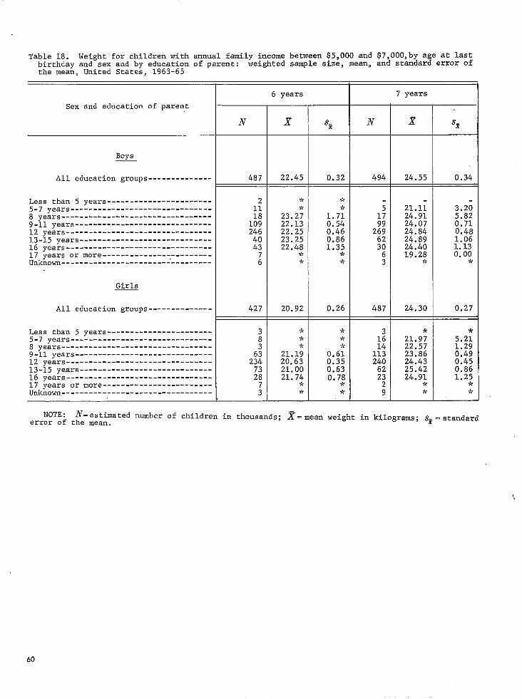
Table 18. Weight for children with annual family income between $5,000 and $7,00O,by age at last birthday and sex and by education of parent: weighted sample size, mean, and standard error of the mean, United States, 1963-65 - -r 6 years T 7 years


N x N x

Boys

All education groups-------------- 487 22.45 0.32 494 24.55 0.34

Less than 5 years----------------------- 2 9< -2

5-7 years _-----_-_---------------------- 11 t 9< 21.11 3.2;8 years--------------------------------- 18 23.27 1.71 24.91 5.82 9-11 years ___------__------------------- 109 22.13 0.54 24.07 0.7112 years-------------------------------- 246 22.25 0.46 24.84 0.48 13-15 years __---_-_----_---------------- 40 23.25 0.86 24.89 1.0616 years-------------------------------- 43 22.48 1.35 24.40 1.1317 years or more---------------,--------- 7? ;ri 19.28 0.00Unknown--------------------------------- ; * 4 * *

Girls

All education groups-------------- 427 20.92 0.26 24.30 0.27

Less than 5 years----------------------- -A A 35-7 years------------------------------- -2 f< 21.9; 5.2:8 years--------------------------------- 4 ii: 1.29 9-11 years------------------------------ 21.19 0.6; 113 ;f%12 years-------------------------------- 20.63 0.35 240 24:43 Ez 13-15 years----------------------------- 21.00 0.63 62 25.42 0:8616 years-------------------------------- 21.74

-k Oa7$j 23 24.91Jc

1.25*17 year- or more------------------------

unknown--------------------------------- f< 9< ; * *

NOTE: N=estimated number of children in thousands; X=mean weight in kilograms; $ =standarderror of the mean.

60

‘

Table 18. Weight for children with annual family income between $5,000 and $7,00O,by age at last birthday and sex and by education of parent: weighted sample size, mean, and standard error of the mean, United States, - 1963-65-Con. - -

8 years T 9 years r 10 years r 11 years

N 8 N x N x N x

439 28.09 0.39 449 32.21 0.56 396 33.97 0.46 422 38.97 0.84 c

b 3 -2 28.0; 3.4; 38.3: 5.3:4’; 28.1; 1.42 30.45 1.98 :z 31.95 10.21 :: 42.7;

86 29.34 1.08 32.13 1.07 102 33.34 0.64 102 38.98 208 27.67 0.67 0.62 166 33.20 0.91 197 37.63

66

E 26.55 0.84 E i 2.00 51 0.89 36 39.43 32.07

* 2.89

t 33128* 2.93

* 16 E! 7.61 40.53

* * 15

4 38:42

* 1.79

* t9741.17

- -

431 26.85 0.48 397 31.57 0.56 406 35.34 0.70 455 40.02 0.55

4 * * * x ;I * 13

16 27.6; 1.9: 35.6: 1.91 43.1; 0.4; 25.3: 0.9: 33.30 1.50 30.84 2.43 1% 37.79 1.83 26.89 0.44 2% 31.25 0.70 35.11 0.66 242 40.57 0.96

1.76 33.08 39 37.73 2.31 2E

* * 1.73

*

29

3”

30.89

* *

0.88

* * 39.87

* %* 13 43.11 10.14

12 45.3: 6.87 ** * 6 * * 3

61

---- --------------

------ ----- -------------

Table 19. Height and weight for children with education of parent equal to 12 years, by age at last birth-day, sex, and annual family income: weighted sample size, mean, and standard error of the mean, .SJnited States, 1963-65

-6 years 7 years

Sex and annual family income

i Height in centimeters All incomes------------------------------

Less than $500---------------------------------$500-$999-------------------------------------$l,ooo-$l,ggg -------____--------_-------------$2,00&$2,ggg -____________---_-__-------------$3,000-$3,ggg---------------------------------$4,000-$4,ggg----------------------------------$5,000-$6,999---------------------------------$7,ooo-$g,ggg --____-____-_----___-------------$10,000~$~4,ggg~~~~~~~~~~~~~~~~~~~-~~~~~~~~~~~~$15,000 or mo=e--------------------------------Don’t know-------------------------------------No response------------------------------------

Girls

Al l incomes------------------------------

Less than $500--------------------------------$g)o-$ggg -____-_______--__--_-----------------$1,000-$1,ggg ---_______--_----___-------------$2,000-$2,ggg -_--___-__--_---_-__-------------$3,000-$3,ggg -__________--------_-------------$4,000-$4,ggg---------------------------------$-j,OOO-$6,999 ____________-_____________________ $7,oo&$g,ggg -____________----________________L $1rJ,ooo-$14,ggg -___ - -___-------_-------_-------$15,000 or mope--------------------------------Don’t know-------------------------------------No response------------------------------------

Boys

Al l incomes------------------------------

Less than $500 ----_-----_----____--------------$5oo-$ggg --_-

871

13 7

27"

1;;246 187 96

2:13

745

165

:6" 45

2::197

E 23

871

13

119.1 0.33

Ekt 1:38 0.770.50

120.1 0.92118.1 1.22

121.5 27.30 113.7 2.28 118.4 2.08 119.6 2.07 117.7 2.17 117.1 0.61 120.5 1.02 117.2 1.18 116.1 2.22 115.7 2.57

-I

828 125.0

; ” * *

5”: 125.: 1.5;126.4 1.6595; 124.6 1.02

269 0.69 228 ;z 0.83

62 124:5 0.84

2 5

123.;*

1.5;*

808 124.0 0.33

**

:;;.i 1.7;2.17

123:9 1.25 124.5 1.34 123.3 0.58

:;1*82 x4‘9c * *

122.4*

1.40* Weight in kilograms

22.32 0.17 24.95

* *

21.4; 2.1; ;

19.9; ;.;g21.74 0.68 5”: 24.57 22.01 0.59 25.70 0:76 21.91 0.45 ;90 24.98 0.95 22.25 0.46 269 24.84 0.48 22.78 0.51 228 25.12 0.54 22.32 62 24.54 0.70 24.13. !E 27.25 6.80 23.88

* I.157 i’;

5 24.72

* 1.37

*t

21.98 0.32 808 24.42 0.27

* * 22.8; 5.6;19.47 1.44 23.6;: 1.6: 20.96 0.87 24.21 1.81 22.63 1.41 0.58 22.66 1.82 2% 0.79 20.63 0.35 24143 0.45 23.49 0.69 24.81 0.50 21.62 1.03 1.09

2.95 fs3.181 5.49 E%. 2.32 23:Otj 1.24

*

$l,ooo-$l,ggg---------------------------------$2,000-$2,ggg---------------------------------$3,000-$3,ggg -________----------_-------------$4,000-$4,ggg----------------------------------$5,000-$6,999---------------------------------$7,ooo-$g,ggg---------------------------------$10,000-$14,ggg --___---------------------------$15,000 or moTe--------------------------------Don't know-------------------------------------No response------------------------------------

Girls All incomes------------------------------

Less than $500---------------------------------$500-$999-------------------------------------$l,ooo-$l,ggg---------------------------------$2,000-$2,ggg-------------------------T-------$3,00()-$3,ggg -_________-___--____-------------$4,0()0-$4,ggg -______-___----___-_--------------$5,r)OO-$6,999 __________________________________ $7,ooo-$g,ggg---------------------------------$10,000-$14,ggg -______-------------------------$15,000 or moTe--------------------------------Don't know -_----___---_No response-----------------------------------

___--__--------- 7

271

1819' 246187

96

268 13

74.5

NOTE: N=estimated number of children in thousands; x=mean; Sn -standard error of the mean.

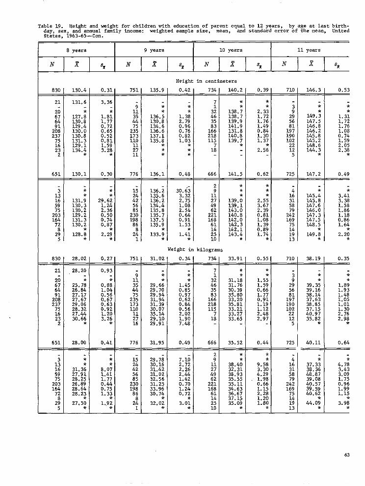
Table 19. Height and weight for children with education of parent equal to 12 years, by age at last birth-day, sex, and annual family income: weighted sample size, mean, and standard error of the mean, United States, 1963-65-Con.

8 years 9 years I 10 years I 11 years

N x % N 8 % N x 54 N x %

Height in centimeters 830 130.4 0.31 751 135.9 0.42 734 140.2 0.39 710 146.3 0.53

- - -21 131.6 3.36 -

* * I * *

* * 191 138.; 2.3;

127.; 1.82 136.; 1.3: 22 138.7 1.72 149.: 1.3;130.8 2 2.79 139.9 1.76 147.5 1.72

5:; Em: 0.96 83: 141.9 1.49 146.8 1.76 3: 0:65 2:; 136:6 0.76 166 131.8 0.84 146.2 1.08

131.3

E2 **

01% 3:28*

110

2 11

135.8* 1.03

* 115

* * 1:* *

139.7*

1.37

2.5: EC6144:3*

2.052.38

*

651 130.1 0.30 776 136.1 0.48 666 141.5 0.62 725 147.2 0.49

5 i63 59

2:: 164

72

289 5

*

131.;

E23 g: p

130:2

128.:*

2.29*

2 42

2;230 198

86

2:1

136.; so.& 135.6 3.32 136.2 2.75 134.4 1.08135.8 2.54 135.7 0.64

0.91i;;*;

'* 1.53

133.9*

1.42*

* *

139.: 139.1

%-ii 142:0142.3 142.1 143.4

*

* *

2.5;3.672.39 0.811.08 1.390.89 1.74

*

145.: 145.8147.6 146.0147.3147.5 148.5

149.;*

;.g 1:58 1.86 1.180.86 1.64

2.2:*

Weight in kilograms

830 28.02 0.27 31.02 0.34 33.91 0.55 38.19 0.35

28.20 0.93 * * 7

1 *

* *

130:8 0.52 173 137.1 0.82 218 140.8 1.30 145.8 0.741.59

1.5; 9;

25.7: 0.8: 29.6; 1.4; 2: 1.59 39.3; 1.8;26.84 1.04 29.70 0.85 0.66 5’: 39.16 1.9327.17 0.56 0.97 i53 35.80 1.77 81 1.48 27.67 0.67 Et 0.62 166 33.20 0.91 197 E-:4; 1.05 29.06 31:39 218 35.81 1.19 190 38185 1.01 28.32 E% 115 1.12 102 37.15 1.30

x 2:02 E:: 2.48 22 2.76 "3% 29: 10 1.90 1: 33:65 2.97 12 43% 2.98

*' * 29.91 7.48 5 - *

651 28.00 0.41 776 0.49 35.52 725 40.11 0.64

* * * *

11 9’

38.4; 9.5: 1: $1;31.3: ;.;2 32.31 3.30 27.91 297 38.93 4.29 538' 3109 28.25 1:77 35.55 . 1.98 1.75 26.89 0.44 2% 35.11 0.66 2;; 0.96 28.64 0.75 1.24 168 1.15 169 1.99 28.23 1.33 0.72 61 2.28 75 1.15

1.20 27.5:

* 1.9;

* 32.0;

* 3.0;

* it 10

1.80*

?G 44.0; *

3.9;*13

L L

63

Table 20. Summary of Daniel's Test for Trend' when either annual family income or education of parent is held constant at the modal class and the other allowed to vary,by age at last birthday and sex: United States, 1963-65

Age and sex

Boys

6 years----------7 years----------

8 year-----------

9 years----------

10 years---------

11 years---------

Girls

6 years----------

7 years----------

8 years----------

9 years----------

10 years---------

11 years--------

'See discussion Significant at

44

High school graduates only,income varying

Height in cm. Weight in kg.T Spear- Spear-Zdi’ man's rs Zdi2 man's rs

34 005952 4 to. 9524 38 0.3214 24 0.5714 98 -0.1667 70 0.1667 32 0.4286 50 0.1071 30 0.4643 20 0.6429 70 -0.2500 54 0.0357

146 -0.2167 62 0.4833 48 0.1429 26 0.5357 40 0.2857 76 -0.3571 74 0.1190 40 0.5238 78 0.0714 94 -0.1190 76 0.0952 78 0.7143

$5,000-$7,000 income only;education varying

Height in cm. Weight in kg.

Spear- Spear-Zdi2 man's rs Zdi2 man's rs

16 0.5429 22 0.3714 4 0.8000 6 0.7000

20 0.4286 18 0.4857 0 +1,0000 4 to.8857

20 0.4286 50 -0.4286 16 0 ‘5429 32 0.0857

4 0.8000 16 0.2000 4 + 0.8857 2 to.9429

24 -0.2000 22 -0.1000 8 0.2000 6 0.4000

36 -0.8000 36 -0.8000 44 -0.2571 36 -0.0286

on I'Test for Trend" in appendix I..05.

---------------------

Table 21. Height and weight for white children living in the central city of an SMSA,by age at last birthday, sex, and annual family income: mean, standard error of the, mean, and weighted sample size, United States, 1963-65

All incomes I

$3,000 Less than $3,000 or more

Age andsex I


6 years--------------------- 118.1 0.64 408 115.1 2.26 48 118.2 0.47 335 7 years--------------------- 124.4 0.75 440 122.0 2.92 57 125.0 0.47 364 8 years--------------------- 129.8 0.51 405 125.8 3.27 45 130.2 0.52 345 9 years--------------------- 135.5 0.85 446 131.3 0.98 51 136.5 0.64 374 10 years-------------------- 139.9 1.32 394 136.3 4.61 52 140.6 1.20 316 11 years-------------------- 146.0 0.65 418 144.0 1.86 59 146.6 0.54 331

Girls

6 years 117.9 0.67 420 118.8 3.25 37 118.2 0.69 356 7 years--------------------- 123.3 0.43 431 120.9 2.81 48 123.6 0.33 371 8 years--------------------- 129.6 0.48 386 126.7 2.92 70 130.3 0.54 29i, 9 years--------------------- 135.5 0.,57 422 130.5 1.95 52 136.5 0.52 349 10 years-------------------- 140.6 0.60 379 136.7 1.57 64 141.4 0.76 299 11 years-------------------- 147.1 0.65 406 * * 21 147.5 0.64 365


6 years--------------------- 21.80 0.461 408 19.91 1.492 48 21.90 0.389 .335 7 years--------------------- 24.67 0.401 440 23.56 1.484 57 24.99 0.341 364 8 years--------------------- 27.78 0.485 405 24.63 1.771 45 28.01 0.477 345 9 years--------------------- 30.28 0.668 446 26.90 1.148 51 30.95 0.671 374 10 years-------------------- 33.97 1.139 394 31.08 5.432 52 34.59 1.064 316 11 years-------------------- 39.12 0.947 418 38.06 1.837 59 39.66 1.039 331

Girls

6 years--------------------- 21.64 0.535 420 21.36 1.951 37 21.80 0.583 356 7 years--------------------- 24.45 0.354 431 23.38 2.511 48 24.49 0.338 371 8 years ---_--------_----__-_ 27.90 0.495 386 25.88 2,059 70 28.34 0.462 294 9 years ---_----------------- 31.82 0.807 422 29.19 2.488 52 32.54 0.858 349 10 years-------------- ____-- 35.26 0.947 379 31.41 2.700 64 36.29 1.069 299 11 years-------------------- 39.87 0.915 406 * * 21 40.04 0.972 365

NOTE: x=mean; $=standard error of the mean; N =estimated number of children in thousands.

6.5

Table 22. Height and weight for white children living on farms of any size in rural areas, by age at last birthday, sex, and annual family income: mean, standard errorof the mean, and weighted sample size, United States, 1963-65

All incomes Less than $3,000 or more Age and sex $3,000

w sz /Xlf Bovs Height in cent io leters

(j years--------------------- 118.6 1.46 133 116.7 1.85 53 120.1 1.83 76 7 years--------------------- 122.8 1.03 140 121.8 27.37 53 124.7 1.34 62 8 years--------------------- 128.7 1.11 141 128.8 3.10 52 128.4 0.75 78 Cj years--------------------- 131.9 2.82 123 133.0 1.60 24 133.4 2.35 81 10 years-------------------- 138.9 1.10 115 138.7 31.07 43 139.1 1.24 63 11 years-------------------- 146.0 1.14 116 144.4 2.82 40 146.7 1.00 72

Girls

6 years--------------------- 117.9 1.26 117 117.8 2.43 36 118.4 1.19 67 7 years--------------------- 122.1 0.95 155 120.8 27.12 48 122.7 1.18 91 $3 years--------------------- 128.5 1.23 137 127.0 2.50 44 129.3 1.51 80 9 years--------------------- 134.6 1.76 127 133.6 2.97 60 135.9 1.22 61 10 years-------------------- 141.1 1.87 146 135.9 3.63 39 143.6 2.22 91 11 years-------------------- 146.1 2.24 128 142.0 3.30 43 149.5 3.55 70


6 years--------------------- 22.38 0.718 133 21.38 3.998 53 23.14 0.784 76 7 years--------------------- 24.29 0.638 140 22.96 5.158 53 26.06 1.101 62 8 years--------------------- 27.27 0.766 141 27.06 2.635 52 27.17 0.723 78 9 years--------------------- 30.36 0.961 123 29.10 1.201 24 31.13 1.469 81 10 years-------------------- 33.24 1.136 115 33.56 7.750 43 32.87 1.458 63 11 years-------------------- 39.16 1.616 116 38.78 3.348 40 39.45 1.172 72

Girls

6 years--------------------- 22.20 0.777 117 21.02 0.584 36 23.19 1.199 67 7 years--------------------- 23.54 0.733 155 22.89 5.215 48 23.96 0.944 91 8 years ---_-- --------------_ 27.63 0.854 137 27.36 2.242 44 27.99 1.208 80 9 years--------------------- 30.40 1.325 127 28.97 2.107 60 32.01 3.982 61 10 years-------------------- 36.72 2.166 146 32.15 4.608 39 38.97 3.058 91 11 years-------------------- 39.35 1.874 128 33.33 2.101 43 44.71 2.908 70

NOTE: x= mean; $=standard error of the mean; N=estimated number of children in thousands.

66

Table 23. Height and weight for white children living in suburban areas,by age at last birthday, sex,and annual family income: qean,standard error of the mean, and weightedsample size, United States, 1963-65

All incomes Less than $3,000 or more$3,000Age and sex


6 years--------------------- 119.3 0.39 622 117.6 3.74 21 119.2 0.42 557 7 years--------------------- 124.9 0.48 606 122.8 5.87 19 125.1 0.50 553 8.years--------------------- 130.3 0.46 600, 127.0 3.19 28 130.4 0.50 547 9 years--------------------- 136.5 0.75 604 136.3 4.38 25 136.7 0.81 528 10 years-------------------- 140.7 0.36 543 140.5 31.57 18 140.8 0.42 501 11 years-------------------- 146.2 0.54 524 147.3 32.97 18 146.1 0.58 483

Girls

6 years--------------------- 118.1 0.32 545 116.4 26.10 20 118.2 0.38 496 7 years--------------------- 124.0 0.35 584 125.6 2.13 19 124.0 0.37 523 8 years--------------------- 129.3 0.38 597 127.0 1.89 35 129.2 0.33 508 9 years--------------------- 136.4 0.65 512 136.6 30.66 20 136.4 0.71 447 10 years-------------------- 141.3 0.56 521 137.5 4.38 25 141.5 0.61 483 11 years-------------------- 147.7 0.56 539 * * 23 147.6 0.66 470

Boys Weigh t in kilograms

6 years--------------------- 22.24 0.199 622 21.70 2.033 21 22.06 0.235 557 7 years--------------------- 24.98 0.307 606 23.87 3.811 19 25.02 0.314 553 8 years---------,------------ 27.94 0.463 600 26.06 1.288 28 28.05 0.462 547 9 years---------------_------- 32.47 1.177 604 31.11 2.852 25 32.39 0.960 528 10 years-------------------- 33.61 0.530 543 35.20 8.427 18 33.68 0.570 501 11 years-------------------- 38.97 0.614 524 41.10 .0.535 18 38.85 0.703 483

Girls

6 years--------------------- 21.83 0.295 545 20.51 4.632 20 21.84 0.275 496 7 years--------------------- 24.59 0.465 58.5 23.99 2.673 19 24.71 0.505 523 8 years--------------------- 27.16 0.402 597 25.48 0.688 35 27.10 0.372 508 9 years--------------------- 32.30 0.719 512 30.20 7.239 20 32.48 0.827 447 10 years-------------------- 35.13 0.674 521 33.17 4.738 25 35.28 0.721 483 11 years-------------------- 39.92 0.518 539 * * 23 39.83 0.771 470

NOTE: X=mean; S.-=standard error of the mean; N=estimated number of children in thousands,.

67

Table 24. LOth, 50th, and 90th percentiles of height and weight distributions of children, by age at last birthday and sex for the following income gr0ups:U.S. tota1,U.S. less than $3,000, U.S. $10,000 or more, and total incomes for India and U.A.R.: United States, 1963-65; India, 1956-65;and U.A.R., 1962-63

-

T Distribution at the 10th percentile

Age and sex U.S. *total

Boys

6 years----------------------------------------

7 years----------------------------------------

8 years----------------------------------------

9 years----------------------------------------10 years---------------------------------------

11 years---------------------------------------

Girls

6 years----------------------------------------

7 years----------------------------------------

8 years----------------------------------------

9 years----------------------------------------

10 years---------------------------------------

11 years---------------------------------------

Boys

6 years----------------------------------------

7 years----------------------------------------

8 years----------------------------------------

9 years----------------------------------------10 years---------------------------------------

11 years -_--_ -_ _---_-_-- _--___-- _-_____________

Girls

6 years----------------------------------------

7 years -_-------_---------_--------------------8 years----------------------------------------

9 years----------------------------------------10 years---------------------------------------11 years---------------------------------------


111.4 110.6 112.7 100.7 106.0 117.0 115.5 120.3 106.1 110.0 122.4 119.8 123.8 111.5 114.7 126.7 125.5 130.2 115.6 119.1 131.2 128.2 132.0 120.4 122.4 136.7 137.4 138.8 124.4 126.3

110.4 108.6 113.0 99.5 105.3 115.7 115.9 117.6 104.8 109.4 121.2 119.6 124.6 109.9 114.1 126.4 125.6 129.1 114.1 118.4 131.5 130.1 135.5 119.5 122.2 138.1 136.4 141.1 123.8 126.8

Weight in kilograms

16.8 17.3 18.4 13.7 16.1 20.2 19.4 21.4 15.1 18.0 21.4 21.6 23.3 16.3 18.9 23.8 22.4 26.4 17.9 20.4 26.3 25.6 27.6 18.5 22.4 30.0 31.1 30.9 20.9 23.7

16.3 16.6 18.5 12.9 15.7 18.7 19.0 20.1 13.8 17.6 21.0 21.2 23.1 15.9 18.8 23.4 23.5 25.3 17.3 20.1 25.9 24.8' 27.2 19.0 22.4 29.7 28.2 32.6 20.7 23.8

age Table 24. lOth, SOth, and 90th percentiles children, at last birthday and sex for the following

of height and weight distributions lessof than $3,000,by U.S.income gr0ups:U.S. total,U.S.$10,000 or more, and total incomes for India and U.A.R.:United States, 1963-65; India, 1956-65; and U.A.R., 1962-63--con.

Distribution at the 50th percentile Distribution at the 90th percentile

U.S. U.S. U.S. less less total than &Aioo India U.A.R. U.S.

than $~&OO India U.A.R. $3,000 or &ore total

$3,000 or more


118.6 116.4 118.9 108.4 114.0 125.9 123.6 126.6 117.2 122.2 124.4 122.5 125.5 114.0 117.8 132.7 132.4 132.8 122.6 126.3 130.0 129.2 130.5 119.8 122.6 137.8 137.8 136.7 129.8 131.2 135.9 133.1 137.1 123.8 127.2 143.9 140.8 145.5 133.0 136.1 140.7 139.0 140.8 128.8 131.7 149.0 147.3 149.1 138.0 141.2 146.0 145.8 146.9 133.3 135.9 154.6 151.8 154.7 143.4 145.1

117.9 116.8 119.1 107.2 113.1 125.1 124.5 123.5 115.9 121.7 123.5 121.8 125.3 113.0 117.1 131.3 129.5 130.7 121.4 126.0 129.7 128.6 130.7 117.8 122.3 137.8 135.3 136.7 127.1 130.7 135.5 134.3 136.5 122.5 126.8 144.9 142.7 146.1 131.5 135.1 141.1 139.1 142.8 128.1 131.5 150.4 149.7 150.6 137.7 141.3 147.4 146.6 147.3 133.4 136.6 157.9 156.5 159.2 144.0 147.3

Weight in kilograms

22.0 20.5 22.0 16.7 20.2 26.8 23.1 26.3 21.1 24.6 24.1 23.1 25.1 18.4 21.2 29.7 28.6 30.8 23.0 25.7 27.1 26.4 26.8 19.6 23.4 34.1 32.5 33.3 23.9 28.8 29.7 28.5 31.2 21.2 25.2 39.2 35.2 39.6 26.0 31.2 32.9 30.6 32.7 i2.9 27.6 42.1 39.4 40.5 28.1 33.9 36.9 35.6 37.5 25.4 30.2 49.3 44.4 47.0 31.6 36.9

21.3 20.7 22.1 15.8 19.9 26.6 23.9 27.2 19.0 24.4 23.6 22.4 25.2 17.3 20.9 29.8 26.6 30.6 21.0 25.7 26.8 25.8 27.7 19.2 23.2 34.7 32.3 34.7 23.4 28.8 29.8 27.7 31.1 21.0 25.0 41.7 37.8 43.7 25.7 31.7 33.9 31.9 36.1 23.2 27.7 45.7 46.4 44.1 28.6 34.5 38.2 37.8 38.8 25.7 30.7 53.1 55.9 51.6 32.9 39.0

69

--

Table 25. Cross-cultural comparisonofage of children upon attaining equivalent height or weight:A. U.S. child in income group of less than $3,000 to U.S. child in income group of

$10,000 or more;1B. U.A.R. child to U.S. child, all incomes;C. Indian child to U.S. child, all incomes,

-

Average

Income group Age of children upon reaching comparable differ-height and weight ence,

all ; ages2

A. U.S., less than $3,000-------- 6.50 7.50 8.50 9.50 10.50 11.50 . . .

U.S., $10,000 or more:

Height, boys--------------- (3) 7.05 8.25 8.90 LO.02 11.32 -0.39 Heigllt, girls-..------------ (3) 6.93 8.11 9.12 9.92 11.34 -0.42 Weight, boys--------------- (3) 6.86 8.23 8.88 9.36 11.11 -0.62 Weight, girls-..------------ (3) 6.60 7.75 8.52 9.65 11.14 -0.77

8. United Arab Republic---------- 6.50 7.50 8.50 9.50 10.50 11.50 . . .

U.S., all incomes:

Height, boys--------------- ( 3) (3) 7.20 8.00 8.80 9.57 -1.61 Height, girls-------------- ( 3) (3) 7.28 8.03 8.83 9.72 -1.54 Weight, boys--------------- ( 3) (3) 7.24 7.85 8.64 9.70 -1.64 Weight, girls-------------.- (3) (3) 7.38 7.93 8.84 9.71 -1.52

C. India------------------------- 6.50 7.50 8.50 9.50 10.50 11.50 . . .

U.S., all incomes:

Height, boys--------------- (3) (3) 6.72 7.40 8.28 9.09 -2.13 Height, girls-------------- (3) (3) 6.51 7.32 8.25 9.16 -2.19 weight, boys--- __-_-_ I'_---- (3) (3) (3) (3) 6.94 7.92 -3.57 Weight, girls-------------- (3) (3) (3) (3) 7.38 8.20 -3.21

'Values in this table were derived from table 24 by determining,for each particular age and sex group, the median height (or weight) of those children in income group of less than $3,000 and estimating by interpolation at what age children in income group a... I 3re than $10,000 attained this height (or weight).

'ihese are the average differences in years, over all. ages, between the two groupsunder consideration when heights (or weights) are equivalent.

?Value could not be interpolated; extrapolation would have been required.

70

APPENDIX I

STATISTICAL NOTES

The Survey Design

The sampling plan of the second cycle of the Health Examination Survey followed a highly stratified, multi-stage probability design in which a sample of the U.S. population (including Alaska and Hawaii) from the ages of 6-11 years, inclusive, was selected. Excluded were those children confined to an institution or residing upon any of the reservation lands set up for the American Indians.

In the first stage of this design, the nearly 2,000 primary sampling units (PSU’s), geographic units into which the United States was divided, were grouped into 357 strata for the use of the Health Interview Survey and the Current Population Survey of the Bureau of the Census and were then further grouped into 40 super-strata for use in Cycle II of the Health Examination Survey.

The average size of each Cycle II stratum was 4.5 million persons, and all strata fell between the limits of 3.5 and 5.5 million. Grouping into 40 strata was done in a way that maximized homogeneity of the PSU’s included in each stratum, particularly with regard to the degree of urbanization, geographic proximity, and degree of industrialization. The 40 strata were classified into four broad geographic regions (each with 10 strata) of approximately equal population and cross-classified into four broad population density groups (each having 10 strata). Each of the resultant 16 cells contained either two or three strata. A single stratum might include only one PSU, only part of a PSU (e.g., New York City, which represented two strata), or several score PSU’s.

To take account of the possible effect that the rate of population change between the 1950 and 1960 census might have had on health, the 10 strata within each region were further classified into four classes ranging from those with no increase to those with the greatest relative increase. Each such class contained two or three strata.

One PSU was then selected from each of the 40 strata. A controlled selection technique was used in which the probability of selection of a particular PSU was proportional to its 1960 population. In the controlled selection an attempt was also made to maximize the spread of the PSU’s among the States. While not every one of the 64 cells in the 4x4x4 grid contributes a PSU to the sample of 40 PSU’s, the controlled. selection technique ensured the sample’s matching the marginal distributions in alI three dimensions and being closely representative of all cross-classifications.

Generally, within a particular PSU, 20 census enumeration districts (ED’s) were selected with the probability of selection of a particular ED proportional to its population in the age group 5-9 years in the 1960 census, which by 1963 roughly approximated the population in the target age group for Cycle II. A similar method was used for selecting one segment (cluster of households) in each ED. Each of the resultant 20 segments was either a bounded area or a cluster of house-holds (or addresses). All the children in the age range properly resident at the address visited were eligible children (EC’s). Operational considerations made it necessary to reduce the number of prospective examinees at any one location to a maximum of 200. The EC’s to be excluded for this reason from the sample child (SC) group were determined by systematic subsampling. If one of the sample children had a twin who was not a sample child, thisother twin was brought in for examination; although the results were recorded for use in a special substudy of twins, thistwinwasnot included in the 7,119 children under the present analysis.

The total sample included 7,417 children 6-11 years old, of which 96 percent were finally examined. These 7,119 examined children were said to represent the 24,000,OOO children in the United States who met the general criteria for inclusion into the sampling universe as of mid-1964.

All data presented in this publication are based on “weighted” observations. That is, data recorded for each

71

sample child are inflated in the estimation process to characterize the larger universe of which the sample child is representative. The weights used in this inflation process are a product of the reciprocal of the probability of selecting the child, an adjustment for non-response cases, and a poststratified ratio adjustment which increases precision by bringing survey results into closer alignment with known U.S. population figures by color and sex for each single year of age 6 through 11.

In the second cycle of the Health Examination Survey the sample was the result of three stages of selection-the single PSU from each stratum, the 20 segments from each sample PSU, and thesample children from the eligible children. The probability of selecting an individual child is the product of the probability of selection at each stage.

Since the strata are roughly equal in population size and a nearly equal number of sample children were examined in each of the sample PSU’s, the sample design is essentially self-weighting with respect to the target population; that is, each child 6-11 years old had about the same probability of being drawn into the sample.

The adjustment upward for nonresponse is intended to minimize the impact of nonresponse on final estimates by imputing to nonrespondents the characteristics of “similar” respondents. Here “similar” respondents were judged to be examined children in a sample PSU having the same age (in years) and sex as children not examined in that sample PSU.

The poststratified ratio adjustment used in the second cycle achieved most of the gains in precision which would have been attained if the sample had been drawn from a population stratified by age, color, and sex and made the final sample estimates of population agree exactly with independent controls prepared by the Bureau of the Census for the noninstitutional population of the United States as of August 1, 1964 (approximate midsurvey point), by color and sex for each single year of age 6 through 11. The weight of every responding sample child in each of the 24 age, race, and sex classes is adjusted upward or downward so that the weighted total within the class equals the independent population control.

A more detailed description of the sampling plan and estimation procedures is included in Vital and Health Statistics, Series 1, Number 5, 1967: “Plan, Operation, and Response Results of a Program of Children’s Examinations,” and in Vital and’ Health Statistics, Series 11, Number 1, 1964: “Cycle I of the Health Examination Survey, Sample Response,” where, in the latter, the techniques used in Cycle1 are similar to those in Cycle II.

Replication and Training for the Measurement

Process

The only good replication data available for the standing height measurement from Cycle II come from the Chicago stand. In this particular replication study 100 of the original 283 children examined were brought back for reexamination. Fifty of these children were originally examined by Caravan I and were reexamined by Caravan II: 4 the other 50 were originally examined by Caravan II and reexamined by Caravan I. As a result of this planning, all replicature comparisons are be-tween observers who were unaware of the original measurements.

The replicate sample was chosen in terms of convenience of transportation to and from the examination center rather than in a strictly random manner. The technicians were specially instructed to use the same procedures as they did in the original examinations.

All body measurements were replicated except for weight. Weight was not replicated because of the 2-week interval between the dates of the original examination and the replicate examination and because of high day-to-day variability of weight.

These data suggest that after accounting for growth there is not more than a J-millimeter average inter-observer difference for the standing height measurement.

This result is consistent with results of another Health Examination Survey that used similar procedures. The data in this other survey (Cycle III) suggest that the inter- and intra-examiner differences found on replication of height measurements of the same subjects had median absolute differences of only 3 or 4 millimeters.

Training and retraining in body measurement techniques were accomplished in several ways. The initial training was given by Dr. Francis E. Johnston, Professor of Anthropology at Temple University, in the pretests conducted in Washington, DC., and Wilmington, Delaware, prior to the beginning of Cycle II. Two formal retraining sessions were held with Dr. Johnston at Philadelphia in November 1963 and at Washington in January 1964. Besides these sessions with Dr. Johnston, there were practice sessions once a month among the technicians supervised by the supervisory staff physician during the dry runs conducted the day before each stand.

Further reduction of interobserver variability was achieved by using the small number of observers who

NOTE: The list of references follows the text.

72

Y

could be well trained. The same four technicians were used throughout the entire survey of 2% years and 7,119 sample children.

Parameter and Variance Estimation

As each of the 7,119 sample children has an as-signed statistical weight, all estimates of population parameters presented in HES publications are computed taking this weight into consideration. Thus, the estimate ofn a population mean *p” is computed as follows: Z’&TXih? ; where X, is the observation or measurement taken on the i th person and W j is the weight assigned to that person.

The Health Examination Survey has an extremely complex sampling plan, and obviously the estimation procedure is, by the very nature of the sample, complex as well. A method is required for estimating the reliability of findings which “reflects both the losses from clustering sample cases at two stages and the gains from stratification, ratio estimation, and post-stratification.“35

The method for estimating variances in the Health Examination Survey is the half-sample replication technique. The method was developed at the U.S. Bureau of the Census prior to 1957 and has at times been given limited use in the estimation of the reliability of results from the Current Population Survey. This half-sample replication technique is particularly well suited to the Health Examination Survey because the sample, although complex in design, is relatively small (7,119 cases) and is based on but 40 strata. This feature permitted the development of a variance estimation computer program which produces tables containing desired estimates of aggregates, means, or distributions together with a table identical in format .but with the estimated variances instead of the estimated statistics. The computations required by the method are simple, and the internal storage requirements are well within the limitation of the IBM 360-50 computer system utilized at the National Center for Health Statistics (NCHS).

Variance estimates computed for this report were based on 20 balanced half-sample replications. A half sample was formed by choosing one sample PSU from each of 20 pairs of sample PSU’s. The composition of the 20 half samples was determined by an orthogonal plan. To compute the variance of any statistic, this statistic is computed for each of the 20 half samples. Using the mean as an example, this is denotedz,, Then the weighted mean of the entire, undividedsample (zji, is computed. The variance of the mean is the mean square deviation of each of the 20 half-sample

eans about the overall mean. Symbolically, +‘ar (x)and the standard error of the mean is simply


the square root of this. In a similar manner, the standard error of any statistic may be computed.

A detailed description of this replicatidbt process is contained in Vital and Health Statistics, Series 2, Number 14, “Replication: An Approach to the Analysis of Data from Complex Surveys,” April 1966, by Philip J. McCarthy, Ph.D.

Standards of Reliability and Precisien

All means, variances, and percentages appearing in this report had to meet certain standards before they could be considered precise, reliable, and suitable for ‘publication.

For reporting means, two basic criteria were used. The first criterion was that a sample size of at least five was required. If this was not the case (e.g., there are only three lo-year-old Negro males coming from families with income between $500-$1 ,OOO),asterisks (*) are used instead of means and standard errors of means in the tables. If, on the other hand, the first criterion of sample size five was satisfied, then the second criterion must have been demonstrated as well. If the coefficient of variation, that is, the standard error of the mean divided by the mean ts,/X 1,was greater than 25 per-cent, the variation with respect to the mean was considered too large and the estimate was neither precise nor reliable enough to meet the standards; the asterieks (*) in the tables denote failure to meet the second criterion.

Where percentages are reported there is only one criterion used and that is that the number of people from which the percentage is calculated was at least 10. An asterisk again points out where this was not the case.

All the procedures described in the discussion to follow utilized certain rules which should be mentioned here. When a mean (or percentage) was considered unreliable, the cell containing the unreliable mean was pooled with an adjacent cell. The mean used in the analysis was thus a weighted mean computedbymultiplying each of the means by its weighted sample size and dividing by the sum of the weightedsamplesizes. Pooling was carried out until all the means reported met the specified criterion for inclusion.

Hypothesis Testing

Several methods of hypothesis testing have been used in the report:

z&x&-If one independent sample is drawn from each of two univariate normal distributions with means pi and p2 a method is sought to test the hypothesis that their means areequal,i.e.,p, = ~~.Thenullhypothesis is HO : p 1= #*with the alternative HA :pl + p2. Ordinarily, to test a hypothesis concerning means from two in-dependent samples, a t-test is done which makes the

73

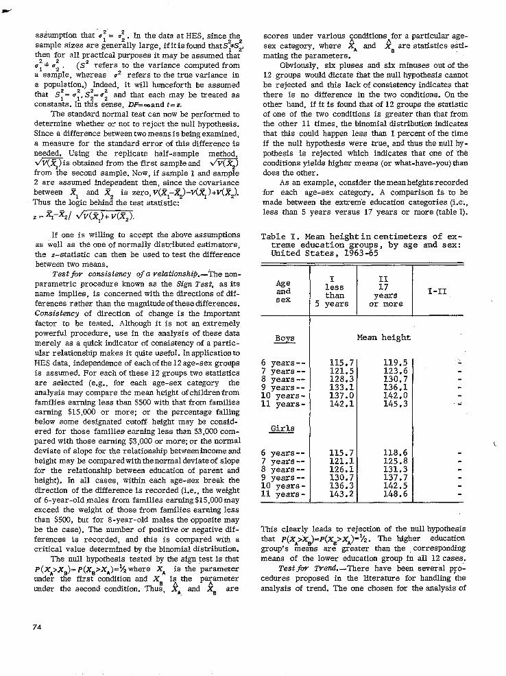
assumption that f~: = V’ . In the data at HES, since the sample sizes are gene&y large, ifitis found thatS~+=S~, then for all practical purposes it may be assumed that

2 2Q1 + u.* . (S2 refers to the variance computed from a sample, whereas g2 refers to the true variance in a population.) Indeed, it will henceforth be assumed that Sf= bz, Si=uz and that each may be treated as constants. In this sense, DF=ooand t-z.

The standard normal test can now be performed to determine whether or not to reject the null hypothesis. Since a difference between two means is being examined, a measure for the standard error of this difference is needed. Using the replicate half-sample method, qis obtained from the first sampleand q from the second sample. Now, if sample 1 and sample 2 are assumed independent then, since the covariance between x1 and Za is zero, V(Zl-Z2)=V(jz)+V(Z,J Thus the logic behind the test statistic:

z = %$I dv(Z*)+ v(Z;).

If one is willing to accept the above assumptions as well as the one of normally distributed estimators, the z-statistic can then be used to test the difference between two means.

Test for consistency of a relationship.-!Che non-parametric procedure known as the Sign Test, as its name implies, is concerned with the directions of differences rather than the magnitude of these differences. Consistency of direction of change is the important factor to be tested. Although it is not an extremely powerful procedure, use in the analysis of these data merely as a quick indicator of consistency of a particular relationship makes it quite useful, In application to HES data, independence of each of the 12 age-sex groups is assumed. For each of these 12 groups two statistics are selected (e.g., for each age-sex category the analysis may compare the mean height of children from families earning less than $500 with that from families earning $15,000 or more; or the percentage falling below some designated cutoff. height may be considered for those families earning less than $3,000 compared with those earning $3,000 or more; or the normal deviate of slope for the relationship betweenincome and height may be compared with the normal deviate of slope for the relationship between education of parent and height), In all cases, within each age-sex break the direction of the difference is recorded (i.e., the weight of 6-year-old males from families earning $15,000 may exceed the weight of those from families earning less than $500, but for &year-old males the opposite may be the case). The number of positive or negative differences is recorded, and this is compared wiG-~ a critical value determined by the binomial distribution.

The null hypothesis tested by the sign test is that P(XA>Xa)= P(XB>XA)=$-2 where X* is the parameter under the first condition and Xs is the parameter under the second condition. Thus, 4 and ia are

scores under various conditions for a particular age-sex category, where 4 and &a are statistics estimating the parameters.

Obviously, six pluses and six minuses out of the 12 groups would dictate that the null hypothesis cannot be rejected and this lack of consistency indicates that there is no difference in the two conditions. On the other hand, if it is found that of 12 groups the statistic of one of the two conditions is greater than that from the other 11 times, the binomial distribution indicates that this could happen less than 1 percent of the time if the null hypothesis were true, and thus the null hypothesis is rejected which indicates that one of the conditions yields higher means (or what-have-you) than does the other.

As an example, consider the mean heights recorded for each age-sex category. A comparison is to be made between the extreme education categories (ile., less than 5 years versus 17 years or more (table I).

Table I. Mean height in centimeters of extreme education groups, by age and sex: United States, 1963 -65

IIAge 1:ss 17 I-IIand than yearssex 5 years or more

Boys Mean height

6 years-- 115.7 119.5 7 years-- 121.5 123.6 8 years-- 128.3 130.7 9 years-- 133.1 136.1 10 years-11 years- Ez*i . "12; .

Girls

6 years-- 115.7 118.6 7 years-- 121.1 125.8 8 years-- 126.1 131.3 9 years-- 130.7 137.7 10 years- 136.3 11 years- 143.2 %Z .

-!-

This clearly leads to rejection of the null hypothesis that p(xAixJ~~(xB>xA)=%. The higher education group's means are greater than the corresponding means of the lower education group in all 12 cases.

Testfor Trend.-There have been several procedures proposed in the literature for handling the analysis of trend. The one chosen for the analysis of

74

------------

data in this report is the nonparametric procedure known as Daniel’s Test for Trend’% which is,in effect, Spearman’s Correlation Test.37 Spearman’s Correlation Test measures the degree of correlation between two numerical variables. In our trend analysis, the first variable is the socioeconomic one under consideration.

In the analyses of the present report, all children within a particular age-sex category are distributed by the appropriate socioeconomic categories. The statistic of interest (be it mean or percentage) is calculated for each socioeconomic category, and the statistic is listed next to the appropriate socioeconomic category (from which it was computed). Obviously, an increasing trend or, put another way, a monotonically increasing relationship between a socioeconomic variable and the variable under consideration could be demonstrated if, as the socioeconomic variable in-creased in magnitude, the statistic representing the variable under consideration increased as well.

To be more specific, within each age-sex category the mean height (or weight) was computed for each income (or education) category. A rank of “1” is assignedz to the lowest income category “less than $500; “2” to the next highest ($500-$l,OOO),and so

on until a rank of “10” is assigned to the highest in-come category “more than $15,000.” This is called the theoredcal rank. Then, if it is hypothesized that as in-come increases so does height, it would be expected that

zRecd here that if die samplesizewere lessthan 5 or if the coefficientof variationsXjXwere greaterthan .2X10,this first groupwouldbe a pooledonewhichdid meetehecriteria(e.g.FSl,OOO).


Table II. Worksheet for Spearman’s Test on income group: United

Income Theoretical rank

Less than $1 ,OOO---------$1,000-$1,999------------ 2'$2,000-$2,999------------$3,000-$3,999------------ 2$4,000-$4,999$5 ,OOO-$6,999 m--M-------- 2$7,000-$9,999------------$10,000-$14,999---------- z$15,000 or more---------- 9

assigning ranks to the means at each level of income would, similarly, show a rank of 1 (indicating the smallest mean) corresponding to the lowest income category and upward until finally the largest mean is observed for the largest income category and is as-signed a rank of 10. At each level of income the value ! d, (difference between the theoretical rank under the null hypothesis and the rank of the mean observed for that income category) is determined. Each d,, is squared and the sum of these squared differences

Q, is calculated. Spearman’s Rank Correlation c:oefficient r* is then computed by the following form

ula: ‘r = 1 A$?$- .. where N=number of categories

of the socioeconomic variable under consideration. Tables are available of the probability distri

bution of various values for r, for different levels of N. Use of *such tables enables tests of the null hypothesis ‘;= 0 against the alternative r,+O. Obviously as N increases, smaller values for rr ‘would be considered significant where they might not have been for smaller values of N. Example: Consider the mean heights corresponding to the various income levels for 6-year-old boys (table II).

Note that&22. Using Spearman’s formula for computing the correlation coefflcient,r*-i-~~~8167. Tables indicate that for N-9 the 99-percent cridcalvalue is 0.783 and the 9%percent critical value is 0.600. Thus a correlation coefficient of 0.8167 indicates that a positive trend does exist-anddoes so with 99-percent confidence.

Weighted leastsquaresasa testfor tvsnd. -If there indeed exists a positive relationship between income

mean heights of 6-year-old boys, by familyStates, 1963-65

Mean II I-II di2height rank dl

l115.2 117.0 5 -1" f117.4 118.5 2 I:: 1"116.8 2 119.5 -? z120.1 9' -2 118.7 :: 119.6 : T 1

I- 0 22 . lThis is a pooled mean, made up of 23 persons, which meets the criteria for preci

sion and reliability. In this case, as is seen in table 1, the mean for the category"less than $500" alone did not meet the criteria and so pooling the first two categories was called for.

75

-------------

(or education) and height (or weight), then a useful test for this relationship would be to fit a regression line to the data to determine the slopeand then to determine whether or not this slope is significantly greater than zero. That is, a regression line of the form Y=a+@,Xi+e, is to be fit ‘to the data where, in this case Y= height (or weight), X= income (or education),a=“Y-intercept,” i.e. ,,value of height (or weight) if income (or education) equaled zero, s = slope of Y on X, i.e., the rate of change in height (or weight) per unit change in income (or education), and finally, e = unexplained error.

The data available from the Health Examination Survey present certain very basic problems which discourage the use of classical regression procedures. Among these problems are violation of the assumptions of independence of the original observations, violation of homoscedasticity, i.e., equal variances of the dependent variable within each category of the independent variable, perhaps violation of the normality assumption, etc. Dr. Paul Levy of the Office of Statistical Methods of NCHS has worked out a “modified regression model which makes no assumptions about the original observations and which makes no stronger assumptions about the sample estimates than are made in testing whether two means are equal when the estimated means and their standard errors are obtained from complex surveys.” 88

The proposed model is as follows: 1. Let F, be the estimated mean and sii be its

estimated standard error for the ith group. 2. Let X, be the midpoint of the independentvari

able for the group.

“aFromanunpublishedmemorandum by Dr. Levy.

3. Assume SF, is based on a largeenoughnumber of observations thdt it can be assumed it is, in fact, equal to ul, and thus has no sampling error.

4. Further assume that

E (ji,,=a+PX, 2V(g,)=Sg, for j-l,? ,... ,K,whereK

is the number of groups. 5. *Finally, it is assumed that the y,% are norm-

ally distributed and they are statistically independentofeachother.

The weighting procedure proposed weights all observations by the reciprocal of thevariance.That is, W,=‘/S& and the mean x= %v,X&~ and the mean Y-+~&.

The slope is computdd in a manner similar to thd classical least squares regression, by’the following formula:

b- zw,(x,-X! q Zw,(X,-X)2

Computationally, this is easily computed by b~;zw,x,~-(~w,)(x)(~)

zw,x:-(zw,)x2 The variance of the slope is

Now, since this formula can be simplified to

zwi(x,-X)’ 1 “~=[zw,(x,-z)2]2 = rw, (x,-X)’

and computationally 1

‘b= JZw,X;-(Cw,)z2

Table III. Worksheet for weighted least squares regression of mean heights of 6-year-old boys, by education of parent: United States, 1963-65

I I I Midpoint

Mean StandardofEducation of education height error of s*-

u, w, = 1/q,parent mean

O-4.99 years--------

5-7.99 years--------8 years

9-11.99 years-------12 years------------

13-15.99 years------16 years-----------

group

2.5 115.7 2.68 7.1824 0.1393

6.5 117.2 .92 .8464 1.1815 8.0 117.8 .86 .7396 1.3521

10.5 117.7 .50 .2500 4.4000 12.0 119.1 .33 .1089 9.1828 14.5 120.4 .71 .5041 1.9838 16.0 118.9 .68 .4624 2.1627

76

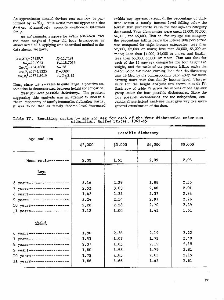
An approximate normal deviate test can now be per-formed by Z= b/Sb. This would test the hypothesis-that B- 0 or, alternatively, compute confidence intervals for B.

As an’example, suppose for every education level the mean height of 6-year-old boys is recorded as shown in table III. Applying this described method to the data shown, we have:

zw,x,q=27859.7 X=11.7191 xw, -20.0022 F&18.7036

~w,x,=234.4068 bc.28 zw, F, =2374.3325 s,=.O897

zw,x,*=2871.3919 z+3.12

Thus, since the z-value is quite large, a positive association is demonstrated between height and education.

Test for best possible dichotomy.--The problem suggesting this analysis was an attempt to isolate a “best” dichotomy of family income level. In other words, it was found that as family income level increased

Table IV. Resulting ratios by a e and sexsidera f ion: United

(within any age-sex category), the percentage of children within a family income level falling below the lowest 10th percentile value for that age-sex category decreased. Four dichotomies were used: $2,000, $3,000, $4,000, and $5,000. That is, for any age-sex category the percentage falling below the lowest 10th percentile was computed for eight income categories: less than $2,000, $2,000 or more; less than $3,000, $3,000 or more; less than $4,000, $4,000 or more; and finally, less than $5,000, $5,000 or more. This was done for each of the 12 age-sex categories for both height and weight, and the ratio of the percent falling under the cutoff point for those earning less than the dichotomy was divided by the corresponding percentage for those earning more than that family income level. The results for the height analysis are shown in table IV. Each row of table IV gives the scores of one age-sex group under the four possible dichotomies. Since the four possible dichotomies are not independent, conventional statistical analyses must give way to a more general examination of the data.

dichotomies under con-for each of the fourStates, 1963-65

-

T Possible dichotomy Age and sex

.Mean ratio---------

Boys

6 years------------------7 years------------------8 years------------------9 years------------------10 years-----------------11 years ----_------_-----

Girls

6 years------------------7 years------------------8 years------------------9 years------------------10 years-----------------11 years-----------------

$2,000 $3,000 $4,000 $5,000

2.00 1.95 2.09 2.03

3.16 2.29 1.88 2.55 2.53 3.03 2.40 2.01 1.42 2.32 2.37 2.33 2.24 2.14 2.97 2.26 2.28 2.28 2.70 2.29 1.18 1.00 1.41 1.61

1.90 2.36 2.19 2.22 1.53 1.07 1.75 1.40 2,.37 1.85 2.19 2.18 1.80 1.58 1.79 1.81 1.75 1.85 2.05 2.15 1.86 1.66 1.42 1.61

77

Table V. Ranks of resulting ratios within each age and sex: United States, 1963-65

Rank Age and sex

$2,000

Mean ratio--------- 29

Boys

6 years------------------

7 years------------------

8 years -_--B---BBw-_--v-_ 9 years------------------10 years-----------------11 years-----------------

Girls

6 years------------------

7 years------------------

8 years------------------

9 years------------------10 years-----------------

11 years-----------------

A preliminary analysis involved obtaining the mean ratio at each possible dichbtomy. As illustrated in table IV the mean ratios for the four. dichotomies are extremely close, and this would lead to the conclusion that each of the possible breaks gives a similardifferentiation. Another tack is to rank the data within each row-the lowest ratio receiving a rank of 1 and the largest a rank of 4. This was done for each of the 12 age-sex categories (table V). If no single dichotomy was better than any of the others, one would expect that summarizing the ranks over all age-sex groups within each of the dichotomies wouldyieldsimilar sums. Alternatively, if one were constantly better than the others, the sum of the ranks would be relatively high since ranks of A should have prevailed within that column. As the above analysis illustrates, the ranks are fairly well distributed and it was felt that the differences among the sums were not large enough to dictate that any one of the

$3,000

24

$4,000 $5,000

33 34

dichotomies was better or worse than any of the others.

A standard nonparametric procedure such as Freedman’s &i-square was not used in this problem because the various dichqtomies are not independent. Thus, an alternative procedure was sought which made no assumption of independence. The W, Statistic de-scribed in “Some Aspects of the Statistical Analyses of the ‘Mixed Model”’ by Gary G. Koch and Pranab Kuma.r Sen which appeared in Biome&$cs, March 1968, is most appropriate here and is based on the ranks described above.

Testing the differences between the various income dichotomies, for heights, ~~d.61 with .3 degrees of freedom, and for weights, w~=I.z~ with 3 degrees of freedom. Since W, is distributed as x * , all dichotomies appear to be performing an equal job of differentiation.

ooo-

78

APPENDIX II

DEMOGRAPHIC VARIAPL

Definitions of Demographic Coding Terms From

HES Procedures Manual

Age.--Age was computed using the date of birth stated at the interview. This was confirmed by comparing it with the date of birth as given on the child’s birth certificate. The age recorded for each child was the age at his last birthday on the date of examination.

NOTE: The age criterion for inclusion in the sample was defined in terms of age on the day of interview. Since the examination usually took place 2 to 4 weeks after the interview some of thosewhowere 11 years old at the time of interview became 12 years old by the time of the examination. There were 72 such cases. In the adjustment and weighting procedures these 72 were included in the ll-year-old group.

Race.-The race classification recorded byobservation was confirmed by comparison with the race classification on the child’s birth certificate. Race was recorded as “white,” “Negro, ‘I or “other.” “Other” included American Indians, Chinese, Japanese, and all races other than white or Negro. Mexicanpersons were included with “white” unless definitely known to be American Indian or of another race. Negroes and per-sons of mixed Negro and other parentage were recorded as “Negro.”

Pare&.-A parent was the natural parent or, in the case of adoption, the legal parent of the child.

Guardian .-A guardian was the person responsible for the care and supervision of the child. He (or she) did not have to be the legal guardian to be considered the guardian in this survey. A guardianship could exist only when neither parent of the child resided in the sample household.

Head of household.- Only one person in each house-hold was designated as the “head.” He (or she) was the person who was regarded as the “head” by the members of the household. In most cases the head was the chief breadwinner of the family although this was not always true. In some cases the head was the parent of the chief earner, or the only adult member of the household.

Household member.+4 household member was a person whose usual place of residence was inthe.-interviewed household. Persons who lived away from their usual place of residence for the purpose of attending school were not considered “household members” at their usual place of residence except during summer vacation periods.

Marital sfatus of parent OY,pardian.--The marital status classification consisted of five major categories: “married,” “widowed,” “divorced,” “separated,” and “never married.” Persons with common-law marriages were considered married. “Separated” was defined as referring only to married persons who had a legal separation or a de facto separation for reasons such as marital discord. Thus, absence of spouse solely because of military service, employment in another location, or similar reasons was not basis for classification as “separated.”

Usual activity of parent or ,pwdian.-This item was defined as that activity (“working,” “keeping house,” or “doing something else”) in which the person had been engaged for most of the time between the date of inter-view and the same date 3 months earlier. “Working” included paid work as an employee for someoneelse for wages, salary, commission, or pay in kind (meals, living quarters, or supplies provided in’place of cash wages). Also included was work in the person’s own business, professional practice, or farm, and work with-out pay in a business or farm run by a relative. Work performed around a person’s own houseor volunteer unpaidwork for a church or charity was not included in the “working” category.

Family income.-The income recordedwas the total income during the past 12 months received by the head of the household and all other household members related to the head by blood, marriage, or adoption. This income was the gross cash income (excluding pay in kind, e.g., meals, living quarters, or supplies provided in place of cash wages) except in the case of a family with its own farm or business, in which case net income was recorded. Also included in the family in-

79

-------

- - - - ---

-----------

come figure were allotments and other money received by the family from a member of the Armed Forces whether he was living at home or not.

Education of parent OY ,guardion.--This item was recorded as the highest grade that had been completed in school, The only grades counted were those which had been completed in a regular school where persons were given formal education in graded or private schools, either day or night schools, with either full-time or part-time attendance. A “regular” school is one which advances a person toward an elementary or high school diploma, or a college, university, or professional school degree. Education in vocational, trade, or business schools outside the regular school system was not counted in determining the highest grade of school completed.

Grade in school (el@ible child).--The grade that the child was attending at the time of interview was taken, The grade of those children on summer vacation was considered to be the grade that they would enter when school resumed.

Geographic region. -For purposes of stratification the United States was divided into four broad geographic regions of approximately equal population. These regions, which correspond closely to those used by the Bureau of the Census, are as follows:

Region States Included

Northeast Maine, New Hampshire, Vermont, Massachusetts, Connecticut, Rhode Island, New York, New Jersey, and Pennsylvania

South _________- _ Delaware, Maryland, District of Columbia, West Virginia, Virginia, Kentucky, Tennessee, North Carolina, South Carolina, Georgia, Florida, Alabama, Mississippi, Louisiana, and Arkansas

Midwest - Ohio, Illinois, Indiana, Michigan, Wisconsin, Minnesota, Iowa, and Missouri

West Washington, Oregon, California, Nevada, New Mexico, Arizona, Texas, Oklahoma, Kansas, Nebraska, North Dakota, South Dakota, Idaho, Utah, Colorado, Montana, Wyoming, Alaska, and Hawaii

Po@.&ztion density. -Four population density groups were used to divide the U.S. population into four approximately equal parts. These groups were de-fined differently for the four geographic regions, in an attempt to obtain a division of each region into the following four classes (1) the largest metropolitan areas; (2) standard metropolitan statistical areas (SMSA’s) of specified size; (3) other SMSA’s or specified highly urban areas; and (4) all other urban and rural areas.

R eg-ion Class Composition

Northeast-------- 1. New York City’s two SMSA’s and the Philadelphia SMSA

2. Other SMSA’s over l,OOO,OOOpopulation

3. Remaining SMSA’s 4. All other urban and rural areas

South_____---__- 1. SMSA’s over 700,000 population 2. All other SMSA’s 3. Specified highly urban areas 4. AI1 other urban and rural areas

Midwest-------- 1. Chicago and Detroit SMSA’s 2. Other larger SMSA’s, most of

them over 500,000 population 3. Remaining SMSA’s 4. All other urban and rural areas

West ______-____ 1. The two Los Angeles SMSA’s and the San Francisco and Seattle SMSA’s

2. AI1 other SMSA’s over 550,000 population

3. Remaining SMSA’s 4. All other urban and rural areas

Urban-rural.--The classification of urban-rural areas was the same as that used in the 1960 census. According to the 1960 definition, those areas considered urban were (a) places of 2,500 inhabitants or more incorporated as cities, boroughs, villages, and towns (except towns in New England, New York, and Wisconsin); (b) the densely settled urban fringe, whether incorporated or unincorporated, of urbanized areas; (c) towns in New England and townships in New Jersey and Pennsylvania which contained no incorporated municipalities as subdivisions and had either 2,500 inhabit-ants or more, or a population of 2,500 to 25,000 and a density of 1,500 persons or more per square mile; (d) counties in States other than the New England States, New Jersey, and Pennsylvania that had no incorporated municipalities within their boundaries and had a density of 1,500 persons or more per square mile; and (e)

80

unincorporated places of 2,500 inhabitants or more which were not included in any urban fringe. The remaining population was classified as rural.

Place description.-The SMSA population was classified as living “in central city” or “not in central city” of a standardmetropolitan statisticalarea (SMSA). The remaining population was classified as “not in SMSA.”

The definitions and titles of SMSA’s are established by the U.S. Bureau of the Budget with the advice of the Federal Committee on standard metropolitan statistical areas.

The definition of an individual standard metropolitan statistical area involved two considerations: First, these must be a city or cities of specified population which constitute the central city and which identify the county in which it was located as the central county; and, second, these must be economic and social relationships with contiguous counties which were metropolitan in character so that the periphery of the specific metropolitan area could be determined.

Persons WI central city” of an SMSA were there-fore defined as those whose residency was in the city or cities of the standard metropolitan statistical area title. Persons who resided in an SMSA but not in the city given in the SMSA title were considered “not in central city.”

The remaining population was allocated into urban (not SMSA), rural-farm, and rural-nonfarm groups. The farm population included all persons living in rural territory on places of 10 acres or more from which sales of farm products had amounted to $50 or more during the preceding 12 months or on places of less than 10 acres from which sales of farm products had

amounted to $250 or more during the preceding 12 months. Other persons living in rural territory were classified as nonfarm. Persons were also classified as nonfarm if their household paid rent for the house but their rent did not include anylandused for farming.

The location number and the 1960 population of the SMSA central cities in the HES sample areshown in the table below.

City Location 1960 number population

Portland, Me------------Boston, ~ss----------Denver, Colo------------Philadelphia, Pa--------Charleston, S. C---------Los Angeles, Calif------Los Angeles, Calif------At-ant-, @-------------San Francisco, Calif----Baltimore, Md-----------New York, N.Y-----------New York, N.Y-----------Minneapolis, Minn-------GrandChicago,

Rapids, Mich------Ill------------

Des Moines, Iowa--------Wichita? Kans-----------Brownsville, Tex--------Houston, Tex------------

Ala---------Birmingham, ~ch-----------Detroit,

Cleveland, Ohio---------Allentown, Pa-----------Newark, N. J-----m--m Jersey City, N.J--------Columbia, S.C-----------

72,566697,197493,887

vg,;;f

2,479:015 487,455740,316934,024

7,781,984 482,872177,313

3,;;;,$$

381: 626 48,040

938,219340,887

1,670,144

APPENDIX III

HOUSEHOLD INTERVIEW QUESTIONNAIRE

CONFIDENTIAL - The National Health Survey is authorized hp Public Law 652 of the 8Jth Congress fill ‘ir.n. 489; 42 U.S.C. 305). AI1 m I ormxion which aould permit identification of the individual will be held strzctlg BUDGET BOREAU NO 68.RblDS, 5 contidcntial, will be used only by pctwns enBaled in and far the pwposcs of the survey and will not be di+ APPRDYAL EXPIRES 1”I.Y JI, 1966 closed ot released to others for any other purposes (22 FR lu37). ~~MN~S-HES-Z U.S. DEPIRTMENT OF COMMERCE 1. Qucsrionnnirc

BYREAU OF THE CENSUSlCTlNC *, COLLECTING *CENT FOR THE

U.S. PuBLtc HE*LTH SERVlCE

NATIONAL HEALTH SURVEY of Qwstionnaircs

. (q) Address or dcscriptian of location (include city, zone, and Stare)

NTA Sc~meot. cnccr:

. (b) Mailing address if not shorn in 2(a) OR n Sa$.e as shown in Z(a) E Serial No. of kern No. by If in NTA Segment

&it also

originalSample Unit which found emct for FIRST

listed on ptopcny

SC~tlWit List Sheet No. Line No.

. (E) Name of special dwelling place ; Code 7. Type of Ii&q quattcrs <Check ona box) i 0 Housing unit 0 Other unit

ALL sc~mcntr (ask if Item 2(a) address identifies a SINGLE-UNIT rttncrute). IO. An thaw any occupied or vacant living quonsrs BESIDES YOUR OWN-

--l” th. bas.m.nt? . . . . 0 Yes--S L--on this floor? . . . . . . . 0 Yes--S L- gI --on eny other floor

of this building? . . . . 0 Yes--S L- 0 No

9. (a) If Own ot Rear free, ask - Do.s this ploee hov. 10 or nlor. *cr.,? ALL se~mcnts (irk if Item ?(a.) idcntificr entire floor ot unnumbered part of

(b) If Rent, ask -Does the place you nnt hove 10 floor in I MULTI-UNIT rtructurc). or mm,. acres?

II. An thwa any accupimd or YDCD~+living quatiers BESIDES YOUR OWN-

If Item 211) identifies entire floor --on this floor? 0 Yes--S L -0 No If Item 2(a) identifies put of the floor,

rm,, T&de x ,a ..Ch qYI,ar. NOT ,,.L.d.,specify patt --in th.--of this floor? I

TA and NTA wgmcnts (ask at al1 units EXCEPT APARTMWT HOUSES). 12. Is ih*r* any other building on this property for p.oplo to live in - eithar occupied

or vacant?

13. What is th. t.lepbona number hen? OR 1m-i No rclcphonc*

INTERVIEWER): If eligible child in household cntct chill i’s nwnc, 14. What would b the best time of day for tha sc,pent srrid, aad column number on luec.lical r*pnsentati** +a corn*?. . . . . . . . . . . . . . . History i%rm.

READ TO RESPONDENT) /1 Medical histories left for-- 1 Person with whamform left-

Column No. and relatwnship

5. RECORD OF CALLS AT HOlJSE3iOLD Item 1 Corn. 2 Corn. 3 CO”?. 4 Corn. 5 CO”l.

D*tc Entire household

Time

6. REASON FOR NON-INTERVIEW ‘YPE A B C z

0 RefusslfD..cdb. ,n ~oomot..~ 0 Vacant--non-seasonal 0 Demolished Interview not obtained for ,oIont 0 No one at home-- 0 Vacant-- seasonal 0 In sample by mistake

repeated calls 0 Usual residence elsewhere 0 Eliminated in sub-sample Cols. - _ _ _ _ 0 Temporarily absent 17) u Other rspaciw u Other Ispec(,y,

because: 0 Other @P.C~IY,

I - I I 7. TYPE A FOLLOW.UP PROCEDURE 18. Signature of intetviewer 19. Code

final 41 results in P Type A non-interview (except RcfusaIs)takc the fallowing steps: 1. Contact neighbors (caretakers, etc.) until you find s~mconc who knows the family. 2. Find out the number of people in the household, their names andap torimate aScs;

If names of all members not known. ascertain relationships. Rccor 3 thts‘. mformarion in the IeSYlar spaces inside the questioansire.

83

1. (a) What is the name of the heod of this household? c~ntsr name I” first column.) (b) What ore the names of all other persons who live here? (L.I~L SII psraona who live here.) (c) I hove listed (Read names) is there myonewlse staying here now such os friends, relatives,,

or roomers? . . . . . . . . . . . . . . . . . . . . . . . . . . . . . . . . . _. . . . . . . . . . . . . . . . . . . . . . . . . . . . . . . 0 Yes (Fiat, 0 No (d) Hove I missed anyone who usually lives hers but is now--Temporarily in a horpitol? 0 Yes (L.,s~) 0 No

__ Away on business? _ . . . . . 0 Yes (~tot) 0 No -_ 0~ a visit or vacation?. . . n Yes &let) 0 No

(e) Do ony of the people in this household hove 01 home mywhae else?

0 Yes (Apply ho”ae*o*d membsrsb~p rolea, If l-ml a ho”eeJlold msmber delete, 0 No (~save on qtxsstiomafre)

2 How o&s)- -related to the hood of the household? mnrer re*ar*anabb to head. for ex.7mo,e: ws3. daudhter. atsImon. liandao”. mo*ber-**-law. *tn*r. room*r’a w,*e, etc.)

4. Sex (Mark one box for each pereon)

5. (a) How old were you on your lost birthday?

For each child age 5-12 listed on the questionnaire, ask: (b) What is the month, day, and year of - - ‘s birth?

(Check with Qusetion s(a) *or conaiatancy)

To Ih 'TERVIEWER: Mark “EC” box for each eligible child (age 6-11) listed on the questionnaire. If no EC, ask coverage questions on Page 1.

NOTE: Questions 6-14 must be asked only of parent(s) or guardian(s) of EC. If no parent or guardian is at home, arrange to call back when they will be home.

Ask oaiy for EC (children 6-11 years of age)

: 5 6. What Is the nome end location of the school --goes to? L

I (a) What grade is - - in?

I Please look q t this card (Hand respondent HES-2(a) card and pencil). 7. Do any of the prestions on that cqd apply to Amy members of the family? Please mark “Yes” or “No”

for each suestion.

(For each “Yes” marked, ask): NOTE: If “I” marked, e,mec name

(a) You have checked- -. Who was this? of hospital ox institution. (b) When was this?

8. Where were you born?

(Check U.S. box or wr*te In nama of oo”“try,

9. Are you primarily right handed, primarily left handed, or both?

! 10. What is the highest grade you attended in school? u. ~Circls h&!hset grads .ttended o* mark ~Won*.‘~,

; (If attended, ask): i (a) Did y?u finish this grads (yeor)?

i( 11. What were you doing most of the post 3 months-working, keeping house, or doing something else?

: (If “Doing somthing else,” ask):

: (a) What were you dolng? (Enter reply verbetim and aak II(b)). . . . . . . . . . . . . . . . . . . . . ._. . . . . . . . . . . . . . . . . . . . 1 - (If “Keeping house” OR “Doing something else,” ask): ; (b) Did you work at o job or business at any time during the past 3 months?. . . . . . . . . . . . . . . . . . . . . . . . . . . . . . . . . : L (If “Working’.’ in 11 OR “Yes” in II(b), ask):

: (c) Did you work full-time.or port&m+?. . . . . . . . . . . . . . . . . .. . . . . . . . . , . . . . . . . . . . . . . . . . . . . . . . . . . . . . . . . . . . . . . .

f 12. Are you now married, widowed, divorced, or rsporatod? (If “Married,” ask): (a) Have you(your husband) boa-a married mae than once?

73. Besides (Read names of children entered in Question 1) hove you md(or) your hurbond(wife) ever hod any other children?

0 Yes 0 No (If “Yes,” ask): (a) What ore their names? (b) How old is--? (c) Where door he(rhe) live now?

-14. Which of these income groups represents your total combined family income fir the post 12 months, that is, your’s, your--‘s, stc? (Show Income Flash Card HES-2(b).) Include income from all rdurces, such as wages,

i soloriss; rents from property, Social Security, or retirement bmefits, help from relatives. etc.

,..,..,.

__-----------First name

Relationship HEAD

3 White 0 Negro 0 Other

7 Male 0 Female

As 0 Under 1 year

Unib

7 EC 0 Not EC

_I No school

Name and location

: I Statement No.

3u.s.

Foreign country

7 Right c] Left

0 Both

i--J None Elem.. . . 12345678 ligh.... 12 3 4 Jolleae 1 2 3 4 5+ --------_____ 7 Yes 0 No 3 Working 0 Keeping hous

0 Something else -----------_-

-----------__ II Yes 0 No ---------____

2 Full-time 0 Parr-rime

7 Married 0 Divorced 7 Widowed 0 Separated------------_ 7 Yes ONo

N*Ille

Group

------------

-------------------------

------------------------- --

Lnsr LIIr ==a-,--_---__---_ _-----------_ -_-~--------_ -------_____ Frrst name First name First name First name First name

1

Relationship Relationship Relationship Relationship Relationship

2 White 0 Negro 0 White 0 Negro 0 White 0 Negro 0 White 0 Negro I-J Other I-J Other 0 Other 0 Other

0 Female 0 Male [7 Female 0 Male 0 Femal .e I-J Male 0 Fern&

0 Under A.9 0 Under Age 0 Under Age n Under 1 year 1 year 1 yea* 1 year

Month Day YeSI Month Day Year

Uonlb I 1 I I

7 EC 0 p; 7 EC 0 !g,r I0 EC u p; 0 EC 0 !g 0 EC 0 p;

7 No school -J No school I-J No school 0 No school 0 No school Name and location Name and location Name and location Name and location Name and location

1

Grade

0 Workins 0 Keeping hous{ 23 Working 0 Keeping hous, :’ re 0 Wdhs 0 Keeping hour 0 Something else

_-----------_ 0 Somedhg else

-------_-_-_ 0 Something else

------------.

_--_-_-~----_ -------_____ I ------------_ -J Yes 0 No --J Yes 0 No [-J Yes 0 No 0 Yes 0 No !J Yes 0 No _--_--r------ -------_---_ --~-------~~------------- ------------_

1 Full-time 0 Pax-rime 7 Full-time 0 Part-rime [1 Full-time 0 Parr-time I

0 Full-time 0 Pm-time

Grade Grade Grade Grade I I

jU.S. 3 u. s. IJTJS. 0U.S. 0U.S.

Foreign country Foreign country Foreign country Foreign country Foreign country

7 Right 0 Left 7 Right 0 Left I 3 Right I-J Left

I-J Both 0 Both 0 Both

0 None I-J None 0 None Elan.. . 12345678 Elan.. . 12345678 Elem.. . 12345678 High... 1234 High... 1 2 3 4 High... 1 2 3 4 College 1 2 3 4 5+ College 1 2 3 4 5+ Colle&e 1 2 3 4 5t ---____-----_ -----------_

Yes 0 No my= ONo I -due;--at,---.

2 Married 0 Divorced 7 Married 0 Divorced 11 Married 0 Divorced 0 Married 0 Divorcee 1 I2 Married 0 Divorced 7 Widowed 0 Separated 7 Widowed 0 Separated _I1 Widowed 0 Separated 0 Widowed 0 Sepatete ,d I7 Widowed 0 Separatecr~es---~-N~--- -------__--__ ------------_

7 Yes 0 No i--J Yes IIN0 0 Yes 0 No I7 Yes UN0 1

Relationship I Year(s) 1 Name of Institution

I I

, , 1 zroup Group GCOIQ WOUP Group

INCOME FLASH CARDS

FORM NHS-HES-2b U.S. DEPARTMENT OF COMMERCE ts-14.63) BUREAU OF THE CENSUS

ACTING AS COLLECTING AGENT FOR THE U.S. PUBLIC HEALTH SERVICE

NATIONAL

Total combined family

Group A.

Group B .

Group C .

Group D .

Group E .

Group F .

Group G .

Group H .

Group I .

Group J .

HEALTH SURVEY

income during past 12 months

. . Under $500 (Including loss)

. . $ 500-G 999

. . $ l;ooo - $ 1,999

. . $ 2,000 - $ 2,999

. . $ 3,000 - $ 3,999

. . $ 4,000'- $ 4,999

. . $ 5,000 - $ 6,999

. . $ 7,000 - $ 9,999

. . $10,000 - $14,999

. . $15,000 and over

USCOMu.oC 15070 P-63

86

15. Is any language other Ifian English spoken here in your home?

0 Yes ON0

(If “Yes,” ask):

what language(s)? Language(s) spoken

(Complete front page of questionnaire)

Comments

rABLE x - LIVING QUARTERS DETERMINATIONS AT LISTED ADDRESS

Are these USE OF CHARACTERISTICS CLASSIFICATION IF HU JN B SEGMENT, ASK (Specify 1oc~tl.m) Occupied All Quarters Not a

. quarters for In what year i2 more lhon one Location of unit Do the

of occu. Do these&ecu,. wz.- =:=a- Fill wsn these (If before July 1760)

j .z ” group of people? (Examples:

pan+* <spa&y

tion) quorierr hove: _ unit

S.Zpatlte @9CCifY loc~tlo*)these question- qwean lO.Zdi.3~) Diner oc- A kitchen (odd naire created?

What was the name of8 Yes NO Basement, quarters live S*SI fmp or cooking occu- and the household head*I J1 IFif1 MO 2nd floor, a.) and eat with ‘ol’,,o,~~;;l’ ;,‘,“fp;,“f pant* btemiew m X9.59 or 1960, of these quarters on fine for any other - to thie sba wasfly -p

z a** group of ;o;;-on riv= us*? quea- ff Hnt half or April 1, 1960?

& &!nwP> psopls? *ion- - *‘L” i* ,a., HU Other h.=W

Ye.3 No Yes No Yes No nafrd .I (2) (3a) (3b) (4) (54 (5b) (64 (6b) (78) ‘(7b) (8) (9~) 7%) (IO) ;11,

FORM NHS-HE%2 IS-IS-c4 “SCOMM-DC I5659 I=63

+dJ.S.GOVERNMENTPRlNTlNGOFFICE: 1977- 260.937:27 87

VITAL AND HEALTH STATISTICS PUBLICATION SERIES

Formerly U.S. Public Health Service Publication No, 1000

Series 1. Progmms and collection procedures.- Reports which describe the general programs of the National Center for Health Statistics and its offices and divisions, data collection methods used, definitions, and other material necessary for understanding the data.

Series 2. Lkata evaluation and methods research .-Studies of new statistical methodology including: experimental tests of new survey methods, studies of vital statistics collection methods, new analydcal techniques, objective evaluations of reliability of collected data, contributions to statistfcal theory.

Series 3. Analvtical studies.--Reports presenting analykal or interpretive studies baeedon vital and health statisucs, carrying the analysis further than the expoaftorytypes of reports in the other series.

Series 4. Documents and committee repoHs. -Final reports of major committees concerned with vital and health statisUcs, and documents such as recommended model vital registration laws and revised l-drth and death certificates.

Series 10. Data from the Health Interview Survev.- Statistics on illness, accidental injuries, disability, use of hospital, medical, dental, and other services, and other health-related topics, based on data collected in a continuing national household interview survey.

series 11. Data from the Health Examination Survey. -Data from direct examination, testing, and measurement of national samples of the civilian, noninstitutional population provide the basis for two types of reports: (1) estimates of the medically defined prevalence of specific diseases in the United States and the distributions of the population with respect to physical, physiological, and psycho-logical characteristics; and (2) analysis of relationships among the various measurements without reference to an explicit finite universe of persons.

S&es 12. &Aa fiorn the Institutional Populrrtion Surveys.-Statistics relating tothe health characteristics of persons in institutions, and their medical, nursing, and personal care received, based on national samples of establishments providing these services and samples of the residents or patients.

Series 13. Data from the Hospital Dischav-ge Survey. -Statistics relating to disch~rrged patients in short-stay hospitals, based on a sample of patient records in a national sample of hospitals.

Series 14. Data on health resources: manpower and facilities. -Statistics on the numbers, geographic distribution, and characteristics of health resources including physicians,dentists, nurses, other health occupations, hospitals, nursing homes, and outpatient facilities.

Ssries 20. Data on mortality.- Various statistics on mortality other than as included in regular annual or monthly reports-special analyses by cause of death, age, and other demographic variables, also geographic and tlme series analyses.

Series 21. Dada on natality, mawiuge, and divorce. -Various statistics on natal&y, marriage, and divorce other than as included in regular annual or monthly reports--special analyses by demographic variables, also geographic and time series analyses, studies of fertility.

Series 22. Lkata fknn the National Natality and Mortality Swveys.- Statistics on characteristics of births and deaths not available from the vital records, based on sample surveys stemming from these records, including such topics as mortality by socioeconomic class, hospital experience in the last year of life, medical care during pregnancy, health insurance coverage, etc.

For a list of titles of reports published in these series, write to: Office of Information National Center for Health Statistics Public Health Service, HRA Hyattsvi&, Md. 20782