hei research report 154. part 3. estimate the effects of air pollution … · part 3 estimating the...

101 Federal Street, Suite 500

Boston, MA 02110, USA

+1-617-488-2300

www.healtheffects.org

R E S E A R C HR E P O R T

H E A L T HE F F E CTSINSTITUTE

Janu

ary 2004

R E S E A R C H R E P O R T


Includes Commentaries by the Institute’s Health Review Committee

Number 154

November 2010

Number 154November 2010

Public Health and Air Pollution in Asia (PAPA): Coordinated Studies of Short-Term Exposure to Air Pollution and Daily Mortality in Four Cities

HEI Public Health and Air Pollution in Asia Program

Part 3

Part 3Estimating the Effects of

Air Pollution on Mortality in Bangkok, Thailand

Nuntavarn Vichit-Vadakan, Nitaya Vajanapoom, and Bart Ostro

with a Commentary by the HEI Health Review Committee

Publishing history: The Web version of this document was posted at


in November 2010.

Citation for whole document:

Vichit-Vadakan N, Vajanapoom N, Ostro B. 2010. Part 3. Estimating the effects of air pollution on mortality in Bangkok, Thailand. In: Public Health and Air Pollution in Asia (PAPA): Coordinated Studies of Short-Term Exposure to Air Pollution and Daily Mortality in Four Cities. HEI Research Report 154. Health Effects Institute, Boston, MA.

When specifying a section of this report, cite it as a chapter of the whole document.

© 2010 Health Effects Institute, Boston, Mass., U.S.A. Asterisk Typographics, Barre, Vt., Compositor. Printedby Recycled Paper Printing, Boston, Mass. Library of Congress Catalog Number for the HEI Report Series:WA 754 R432.

Cover paper: made with at least 55% recycled content, of which at least 30% is post-consumer waste; freeof acid and elemental chlorine. Text paper: made with 100% post-consumer waste recycled content; acid free;no chlorine used in processing. The book is printed with soy-based inks and is of permanent archival quality.

C O N T E N T S

INVESTIGATORS’ REPORT by Vichit-Vadakan et al. 231

ABSTRACT 231

INTRODUCTION 232

SPECIFIC AIMS 233

DATA AND METHODS 233

Data 233Mortality Data 233Air Pollution Data 234Meteorologic Data 234

Methods 234

RESULTS 235

Descriptive Analysis 235

Analytic Results 239

Sensitivity Analyses 245

DISCUSSION 251

ACKNOWLEDGMENTS 253

REFERENCES 254

APPENDIX A. Technical Summary 255

APPENDIX B. Correlations of Pollutants 256

APPENDIX C. Time-Series Plots of Air Pollution 260

APPENDIX D. Lag Effects of PM10 and Gaseous Pollutants 263

APPENDIX E. HEI Quality Assurance Statement 267

ABOUT THE AUTHORS 267

OTHER PUBLICATIONS RESULTING FROM THIS RESEARCH 268

ABBREVIATIONS AND OTHER TERMS 268

COMMENTARY by the Health Review Committee 269

BACKGROUND 269

SPECIFIC AIMS 269

DATA SOURCES 270

DATA ANALYSIS 270

RESULTS 270

Daily Mortality and Pollutant Information 270

Associations Between Daily Mortality and Individual Pollutants 271

HEI EVALUATION OF THE STUDY 272

Assessment of Health Outcomes 272

Pollutant Concentration Monitoring and Exposure Estimation in Bangkok 272

Statistical Methods 273

Epidemiologic Aspects 273

Research Report 154, Part 3

CONCLUSION 275

ACKNOWLEDGMENTS 275

REFERENCES 275

INVESTIGATORS’ REPORT

Part 3. Estimating the Effects of Air Pollution on Mortality in Bangkok, Thailand

Nuntavarn Vichit-Vadakan, Nitaya Vajanapoom, and Bart Ostro

Faculty of Public Health, Thammasat University, Klongluang, Pathumthani, Thailand (N. V-V., N. V.); Office of Environmental Health Hazard Assessment, California Environmental Protection Agency, Oakland, California (B.O.)

ABSTRACT

While the effects of particulate matter (PM*) on mortal-ity have been well documented in North America andWestern Europe, considerably less is known about itseffects in developing countries in Asia. Existing air pol-lution data in Bangkok, Thailand, indicate that airborneconcentrations of PM � 10 µm in aerodynamic diameter(PM10) are as high or higher than those experienced inmost cities in North America and Western Europe. At thesame time, the demographics, activity patterns, and back-ground health status of the population, as well as thechemical composition of PM, are different in Bangkok. It isimportant, therefore, to determine whether the effects ofPM10 on mortality occurring in this large metropolitanarea are similar to those in Western cities.

The quality and completeness of Bangkok mortality datahave been recently enhanced by the completion of a fewmortality studies and through input from monitors cur-rently measuring daily PM10 in Bangkok. In this analysis,we examined the effects of PM10 and several gaseous pol-lutants on daily mortality for the years 1999 through 2003.Our results suggest strong associations between severaldifferent mortality outcomes and levels of PM10 and sev-eral of the gaseous pollutants, including nitrogen dioxide(NO2), nitric oxide (NO), and ozone (O3). In many cases,

Health Effects Institute Research Report 154 © 2010

This Investigators’ Report is one part of Health Effects Institute ResearchReport 154, which also includes a Commentary by the Health ReviewCommittee. Correspondence concerning the Investigators’ Report may beaddressed to Dr. Nuntavarn Vichit-Vadakan, Faculty of Public Health,Thammasat University, Rangsit Campus, Klongluang, Pathumthani 12121,Thailand.

The PAPA Program was initiated by the Health Effects Institute in part tosupport the Clean Air Initiative for Asian Cities (CAI-Asia), a partnershipof the Asian Development Bank and the World Bank to inform regionaldecisions about improving air quality in Asia. Additional funding wasobtained from the U.S. Agency for International Development and the Wil-liam and Flora Hewlett Foundation. The contents of this document have notbeen reviewed by private party institutions, including those that support theHealth Effects Institute; therefore, it may not reflect the views or policies ofthese parties, and no endorsement by them should be inferred.

*A list of abbreviations and other terms appears at the end of the Investiga-tors’ Report.

the effect estimates were higher than the approximately 6%per 10 µg/m3 typically reported in Western industrializednations—based on reviews by the U.S. Environmental Pro-tection Agency (U.S. EPA) and the World Health Organiza-tion (WHO) (Anderson et al. 2004). For example, the excessrisk (ER) for mortality due to all natural causes was 1.3%(95% confidence interval [CI], 0.8 to 1.7), with higher ERsfor cardiovascular and respiratory mortality of 1.9% (95%CI, 0.8 to 3.0) and 1.0% (95% CI, �0.4 to 2.4), respectively.Of particular note, for this warm, tropical city of approxi-mately 6 to 10 million people, is that there is no covariationbetween pollution and cold weather, with its associatedadverse health problems. Multiday averages of PM10 gener-ated even higher effect estimates. Our analysis of age- anddisease-specific mortality indicated elevated ERs for youngchildren, especially infants with respiratory illnesses, chil-dren less than 5 years of age with lower respiratory infec-tions (LRIs), and people with asthma. Age-restricted anal-yses showed that the associations between mortality due toall natural causes and PM10 concentration increased withage, with the strongest effects among people aged 75 yearsand older. However, associations between increases inPM10 concentration and mortality were observed for allof the other age groups. With a few exceptions, relativelysimilar results were observed for several of the otherpollutants — sulfur dioxide (SO2), NO2, O3, and NO,which were highly correlated with PM10. However, manyof the effects from gaseous pollutants were attenuated inmultipollutant models, while effects from PM10 appeared tobe most consistent. In addition, there was some evidenceof an independent effect of O3 for certain health outcomes.

We conducted substantial sensitivity analyses to exam-ine whether our results were robust. The results indicatedthat our core model was generally robust to the choice ofmodel specification, spline model, degrees of freedom (df)of time-smoothing functions, lags for temperature, adjust-ment for autocorrelation, adjustment for epidemics, andadjustment for missing values using centered data (see thedescription of the centering method used in the CommonProtocol found at the end of this volume). Finally, the

231

Part 3. Mortality Effects of Air Pollution in Bangkok, Thailand

concentration–response functions for most of the pollut-ants appear to be linear. Thus, our sensitivity analysesresults suggest an impact of pollution on mortality inBangkok that is fairly consistent. They also provide sup-port for the extrapolation of results from health effectsstudies conducted in North America and Western Europeto other parts of the world, including developing countriesin Asia.

INTRODUCTION

Compelling epidemiologic evidence indicates that expo-sure to current levels of ambient, airborne PM in NorthAmerican and Western European cities is associated withpremature mortality and a wide range of morbidity out-comes (WHO 2000; U.S. EPA 2004). Existing air pollutionmonitoring information and recent exposure assessmentssuggest that airborne PM concentrations in Bangkok andother major Asian cities are as high as or higher than thosein North American and Western European cities. A recentreview of Asian cities, mostly undertaken in developingcountries, suggests that PM may also be associated withboth mortality and morbidity (HEI International ScientificOversight Committee 2004). However, PM chemical com-position and relevant population characteristics, such asactivity patterns, background health status, and other fac-tors related to lower socioeconomic status, all may contrib-ute to differential risks in developing countries such asThailand, China, and India. More specifically, it has notbeen clearly documented whether or to what extent PM-associated human health effects are occurring in Bangkok,the capital and largest city in Thailand. In addition, mostof the studies in developing countries have relied onincomplete data of unknown quality. Therefore, decisionmakers seeking replication of North American and West-ern European results in their own cities and countries maybe hesitant to draw inferences from previous studies. As aresult, the Health Effects Institute embarked on the PublicHealth and Air Pollution in Asia (PAPA) project in order toexamine the effects of PM10 and other pollutants inBangkok and three Chinese cities (Hong Kong, Shanghai,and Wuhan).

Three previous studies have been conducted in Bangkok(Ostro 1998, 2000; Vajanapoom 2002). In an initial effort,Ostro and colleagues (1998, 1999) examined counts ofdaily mortality in Bangkok from 1992 through 1995 andreported a consistent association between PM10 and totalcardiovascular and respiratory mortality, as well as mortal-ity among certain age groups. For that analysis, however,daily data on PM10 were limited and of questionable qual-ity. As a result, concentrations of PM10 were estimated

232

from daily measurements of airport visibility. Since then,the air quality monitoring efforts for the Bangkok Metro-politan Region have been greatly expanded and improved,making them better able to address exposure issues for epi-demiologic research. The Pollution Control Departmentwithin the Ministry of Natural Resources and Environmentcurrently has five ambient and seven roadside air pollu-tion monitoring stations that measure daily PM10 and gas-eous pollutants. These monitors are located throughoutthe metropolitan area and have been operating since 1996.The resulting air quality data show that PM10 concentra-tions in Bangkok remain high and exceed both the annualand 24-hour standards set by Thailand, the United States,and WHO. Although PM10 concentrations decreased dur-ing the economic recession of 1997 and trended down-ward through 2001, they have risen during the last fewyears as the economy has recovered.

The daily mortality data used in the study by Ostro andcolleagues (1999) were gathered and processed through anewly computerized system, and large periods of datawere lost or of questionable quality because of the transi-tion from a manual to on-line computerized system, whichrequired adapting to new procedures and training of staff.Currently, the death reporting system is completely online,and the transitional period ended 3 years before our studyperiod, so the data quality is assured. An online reportingsystem links each death notification, which is registeredat the local registrar’s office by the deceased’s relative, tothe Central Registrar Office. There all death notificationsfrom local offices throughout Thailand are compiled into ausable database. Therefore, daily mortality data are com-plete, quality controlled, and readily available.

The 6 to 10 million residents of Bangkok are poten-tially exposed to high concentrations of PM10. Two ques-tions remain: first, whether they are adversely affectedby the existing concentration levels of PM10 and, second,whether the impact per unit of PM10 concentration (µ/m3)is similar to what is experienced in developed Westerncountries. The improvement in the collection system formortality data and the expanded air monitoring programprovided an excellent opportunity to reexamine the effectsof PM10 and several gaseous pollutants on daily mortalityfor the years 1997 through 2003. In undertaking thisproject, we sought to expand the literature documentingthe effects on mortality of ambient air pollution by addinga study in an Asian city. Our work in Bangkok may be par-ticularly important since Bangkok is a warm, tropical city,and there is no covariation and potential confoundingbetween pollution and cold weather, with its associatedadverse respiratory problems. Therefore, we were able totest the association between PM and health essentiallywithout the confounding effects of most weather factors.

N. Vichit-Vadakan et al.

Of equal importance, we sought to add to the small body ofliterature documenting the health effects of air pollution indeveloping countries, particularly on the Asian continent.

Since our research team included investigators from bothThailand and the United States, an additional objective ofour work was the transfer of technical knowledge fromAmerican to Thai investigators regarding data collection,data analysis, and the quantitative assessment of healthoutcomes. Ultimately, we hope this effort will be useful infostering additional epidemiologic inquiries into air pollu-tion in Thailand and will aid Thai decision makers in deter-mining priorities among many competing environmentaland nonenvironmental issues that affect public health.

SPECIFIC AIMS

Our study took advantage of the improved sources ofdata available to test several specific hypotheses. First,using improved data on PM10 (as well as data on gasessuch as O3, NO2, and SO2) and mortality, we tested for anassociation between ambient air pollution and mortality inBangkok. For this effort, both the mortality and air pollu-tion data went through a rigorous quality assurance andcontrol program administered by HEI. Second, we exam-ined associations between air pollution and both disease-and age-specific mortality, in order to identify potentialsubgroups at particular risk. Finally, we conducted exten-sive sensitivity analyses of the results in order to examinethe influence of model specification, smoothing methods,lag structure, and copollutants.

DATA AND METHODS

DATA

In this study, three basic categories of data were collected:(1) mortality data, (2) air pollution data, and (3) meteoro-logic data. All three databases were compiled electroni-cally by the responsible government agencies, as describedin the next few sections.

Mortality Data

Currently, under the administration of the Bureau ofRegistration Administration, the reporting system fordeaths is entirely online and computerized with no man-ual recording of death certifications or cause of death. TheBangkok Metropolitan Region has a population of around6 to 10 million people, with about 100 deaths per day.Available data used in this study for each individual death

included date of death, age and sex of deceased, andcause of death. We compiled the data for individual deathsfrom June 1, 1997, to May 31, 2003, in order to determinethe total number of deaths each day in Bangkok, as well asthe number of deaths in various disease- and age-specificcategories.

During evaluation of the data quality, we observed sig-nificantly lower death counts for 1997 and 1998 than forthe rest of the study period (1999 to 2003). In order todetermine whether the variations we found were system-atic or random, we examined the distribution of deaths bydistrict and validated the results with the local hard copyof death confirmation records, which is a carbon copy ofthe printout of the death certificate kept at the local regis-trar’s office. The results show that 4 out of 50 districts(districts 4, 8, 17, and 37) had death counts that were dif-ferent from those recorded in the 1997 and 1998 databaseswe received from the Ministry of Public Health, with amuch higher number of deaths in the local hard copydatabase. To avoid these discrepancies, we used only datafrom 1999 to 2003, thereby deviating from our originalstudy plan.

The Ministry of Public Health currently uses the tenthrevision of the International Classification of Diseases(ICD-10) to categorize cause of death. All deaths must becertified by a physician, and the primary cause and under-lying cause of death are recorded on a temporary death cer-tificate by attending physicians at hospitals. Relatives ofthe deceased must submit the temporary death certificateto the local Registrar Office, and in turn, the RegistrarOffice issues an official death certificate.

As mentioned earlier, the system for reporting deaths isentirely computerized, and both the primary causes andunderlying causes of death are recorded as they appearedon the official death certificate. The database is then sent tothe Ministry of Public Health for assignment of the ICD-10code. Thus, consistency in the classification of causes andunderlying causes of death is maintained.

We subtracted from the total mortality count accidentsand homicides, leaving deaths from “natural/nonaccidental”causes (ICD-10 codes A00–R99) — more specifically,deaths due to respiratory-specific causes (J00–J98) andcardiovascular-specific causes (I00–I99); and deaths fall-ing into some additional subcategories, including deathsfrom ischemic heart disease (I20–I25), conduction disorders(I44–I49), LRIs (J10–J22), chronic obstructive pulmonarydisease (COPD) (J40–J47), asthma (J45–J46), and senility(R54). We also examined two control groups: (1) thosewho died from natural, non-cardiopulmonary causes; and(2) those who died from accidental causes. Although senil-ity is not usually considered in time-series mortality

233


studies, we examined this cause of death because our pre-liminary analysis showed a relatively low number of dailydeaths from cardiovascular diseases. We hypothesized thatthis might have been a result of mislabeling the cause ofdeath as being senility rather than cardiovascular disease,especially when an elderly person died outside the hospi-tal. In those cases, the cause of death may have been diag-nosed as senility by a nonphysician coroner. We includedthis hypothesis of possible misdiagnosis in our investiga-tion. We also examined mortality stratified by sex and byage for the following age groups: 0 to 4 years, 5 to 44 years,18 to 50 years, 45 to 64 years, more than 50 years, morethan 65 years, and more than 75 years.

Air Pollution Data

The Pollution Control Department manages the airpollution monitoring in Thailand. Standard methods rec-ommended by the U.S. EPA are used in measuring air pollu-tion. In Bangkok, there are five ambient and seven roadsidemonitoring stations that have been measuring hourlyambient levels of PM10 since 1996; ten stations that havebeen measuring hourly ambient NO2, SO2, and NO since1995; and eight stations that have been measuring hourlyambient O3 since 1997. We carefully reviewed the moni-toring data and picked sites based on consistency, lackof outliers, and completeness. In addition, we used onlythose monitors that met the site selection criteria, speci-fically, those that were not in the immediate vicinity oftraffic or industrial sources and were, therefore, not over-influenced by local sources (e.g., highways, industries, andopen burning). As a result of these criteria, designed toavoid mismeasurement and overestimation of PM10 expo-sure, we did not use any of the available roadside monitor-ing stations since their measurements are unlikely to berepresentative of general population exposure.

To ensure the representativeness of the daily air pollu-tion data, days with fewer than 18 hourly readings wereconsidered ineligible and therefore excluded from the anal-yses. We calculated 24-hour averages for NO2, NO (usingthe difference between NOX and NO2), SO2, and PM10,with the requirement that at least 75% of the 1-hour valuesbe available on that particular day. For the 8-hour averagevalue of O3, at least six hourly values from 10 am to 6 pmhad to be available, since the maximum O3 levels alwaysoccur during daylight (Mikkelsen et al. 2000; Mair et al.2002; Tao et al. 2004; Reddy 2008). The daily concentra-tions for each pollutant used in the analysis were calcu-lated by taking the mean of the measurements from allavailable monitoring stations. We used only the stationswith a completion rate of at least 75% of the measure-ments over the study period. With this criterion, the data

234

completion rate for all pollutants was 100%, except forPM10, which had 4 ineligible days due to missing data.

Averaging the pollutant concentrations over all monitor-ing stations provided the best representation of populationexposure to air pollution for several reasons: First, the Pol-lution Control Department strategically placed the moni-toring stations (five stations for ambient PM10; ten for NO2,SO2, and NO; and eight for O3) over an area of 1600 km2

throughout Bangkok in order to capture exposures over theentire metropolitan area. However, two-thirds of thesemonitoring stations were situated within the inner cityarea, comprising approximately 300 km2, where most ofBangkok’s 6 to 10 million residents live; this area has agreater population density than the outer rim of the city.Second, many Bangkok residents work outside of theirhomes. Many offices are located in the inner city, and resi-dents must travel to their workplaces on a daily basis.Therefore, averaging pollutant concentration measurementsacross various stations rather than measuring concentra-tions only at selected stations can capture the variation inpopulation exposure over time and space. Moreover, mosttime-series studies of major metropolitan areas have adopteda similar approach.

Meteorologic Data

Daily weather data collected at the Don Muang Airportweather station and the Bangkok metropolitan weather sta-tion (at the Queen Sirikit National Convention Center)were available for the study period. The data obtainedincluded average daily temperature and average daily rel-ative humidity (RH). Daily weather variables at the twoBangkok locations were found to be highly correlated witheach other (Ostro et al. 1999). We chose to use the datafrom the Bangkok metropolitan weather station, whichwere more complete (100%).

METHODS

To assess the short-term effects of PM10 and gaseouspollutants on daily mortality, we followed the CommonProtocol developed by participants in the PAPA project,which included research teams representing Bangkok,Hong Kong, Shanghai, and Wuhan (see the Common Proto-col at the end of this volume). We applied generalized lin-ear models using a Poisson regression, conditional on sev-eral independent variables, in order to control for temporaltrends and meteorologic conditions. In the basic analyticapproach, we employed natural cubic spline models usingthe statistical software package R, version 2.5, with mgcv,version 1.3-24 (R Development Core Team 2007, Vienna,Austria). A natural spline model uses a parametricapproach that fits cubic functions together by joining them


Table 1.

Average Daily Mortality by Sex and Age in Bangkok from January 1, 1999, to December 31, 2003

a

Deaths per DayMean (SD)

Sex

Male 61 (8.9)Female 43 (7.6)

Age (yr)

< 5 3 (1.8)5–44 29 (5.9)18–50 34 (6.4)

45–64 27 (5.4)50+ 66 (9.9)65+ 45 (7.9)75+ 21 (5.2)

a

Definition: SD indicates standard deviation.

at knots, which are typically placed evenly throughoutthe distribution of the variable of concern (e.g., time). Thenumber of knots used determines the overall fit for thetemporal smoothing function. Before entering measure-ments of an air pollutant into the model, we used this tech-nique to determine the best core model for all mortalitiesattributed to natural causes, while controlling for time,season, temperature, RH, day of the week, and whetheror not it was a public holiday. This was undertaken tocontrol for factors, besides air pollutants, that vary on adaily basis and that might explain variations in daily mor-tality. Same-day exposure to the air pollutants, single-daylags up to five days, and moving averages of up to five dayswere examined.

All studies in the PAPA project examined a core analyticmodel, which employed 4 to 6 df per year for the smoothfunction of time and 3 df for the whole study period for thesmooth function of the same-day lag of daily mean temper-ature and daily mean RH. The number of degrees of free-dom used has been shown in many previous studies toprovide adequate control for these potential confounders(HEI 2003). Nevertheless, we conducted a sensitivity anal-ysis by considering as many as 15 df for time per year. Thebest core model and number of degrees of freedom for thesmooth function of time were chosen to minimize serialcorrelation. Specifically, we used the criterion of minimiz-ing the absolute magnitude of partial autocorrelation func-tion (PACF) values, with an additional requirement thatthe first-order autocorrelation (AR1) and the second-orderautocorrelation be less than 0.1. The PACF measures theabsolute value of autocorrelation for lags from 1 to 30 days.We used a quasi-Poisson option in the regression modelsto correct for any overdispersion in the data.

In the sensitivity analysis, we assessed the possibilitythat an influenza epidemic could be a potential con-founder of the associations. Unfortunately, daily deathcounts for influenza in Bangkok were likely to be under-reported, so we defined an influenza epidemic as existingwhen the weekly respiratory mortality counts were greaterthan the 90th percentile of the mean frequency (count) ofrespiratory mortality for the given year. We also used sen-sitivity analyses to assess the impact of different modelspecifications on our results. We included models with var-ious sets of degrees of freedom for time and weather andwith different lags for temperature and RH, using penal-ized spline smoothing functions for time and weather inplace of natural splines with the same degrees of freedom.We included autoregressive terms in the model whereappropriate. We also fit copollutant models assessing theeffects of PM10 with adjustments for gaseous pollutants,and vice versa.

RESULTS

DESCRIPTIVE ANALYSIS

Tables 1 to 3 summarize the daily mortality data inBangkok from January 1, 1999, to December 31, 2003. Therewas an average of 95 deaths per day from mortality due toall natural causes. About 8% and 14% of the total con-sisted of mortality from respiratory and cardiovascular dis-eases, respectively, and about half of the total involvedthose aged 65 and older. This study showed that malesmade up about 64% of the total mortality in Bangkok,although a lower proportion of men (48%) were living inBangkok during the study period (Bangkok MetropolitanAdministration 2003). The mean number of deaths per dayfor various causes of death did not change much whenstratified by seasons (Table 3), indicating that season isunlikely to be an effect modifier for the Bangkok data. Thelong-term trends of daily mortality from all natural causes(for all ages and among those aged 65 and older), cardio-vascular causes, and respiratory diseases over the studyperiod are shown in Figure 1. We observed extremely lowdeath counts on December 31 in 1999 and 2000. It is likelythat these outliers were caused by an error in the datarecording process.

The mortality data for Bangkok during this time periodshows slightly increasing trends without apparent seasonalpatterns. This evidence is quite different from that usuallyobserved in temperate regions, where mortality peaks dur-ing the winter months, suggesting that time and seasonalitymay not be strong confounding factors for the acute effects

235

236


Table 3.

Average Daily Mortality by Cause of Death and Seasons in Bangkok from January 1, 1999, to December 31, 2003

a

Cause of Death(All Ages)

Season

SummerMean (SD)

WinterMean (SD)

RainyMean (SD)

All natural 97 (12.0) 95 (10.9) 94 (13.4)Cardiopulmonary 21 (5.5) 22 (5.6) 22 (5.5)Cardiovascular 13 (4.3) 14 (4.2) 14 (4.2)

Ischemic heart diseases 4 (2.1) 4 (2.4) 5 (2.2)Stroke 5 (2.5) 5 (2.5) 6 (2.5)Conduction disorder 1 (0.5) 1 (0.5) 1 (0.4)

Respiratory 8 (3.0) 8 (3.2) 8 (3.1)COPD 2 (1.0) 2 (1.1) 2 (0.9)LRI 4 (2.2) 5 (2.3) 4 (2.3)LRI < 5 yr 1 (0.3) 1 (0.5) 1 (0.2)Respiratory < 1 yr 0.1 (0.3) 0.1 (0.4) 0.1 (0.4)

Asthma 1 (0.4) 1 (0.4) 1 (0.4)Senility 14 (3.9) 11 (4.2) 12 (4.2)Non-cardiopulmonary and

natural (others) 76 (10.3) 73 (9.6) 72 (11.0)Accidental 3 (1.8) 3 (1.7) 3 (1.7)

a

Definitions: COPD indicates chronic obstructive pulmonary disease; LRI indicates lower respiratory infection; SD indicates standard deviation.

Table 2.

Distribution of Daily Mortality by Cause of Death in Bangkok from January 1, 1999, to December 31, 2003

a

Cause of Death (All Ages)ICD-10Codes

Percentiles

Mean Minimum Maximum SD 25 50 75 100

All natural A00–R99 95 29 147 12.1 87 95 103 147Cardiopulmonary I00–I99,

J00–J9822 5 47 5.7 18 21 25 47

Cardiovascular I00–I99 14 1 28 4.3 10 13 16 28Ischemic heart diseases I20–I25 4 1 16 2.3 3 4 6 16Stroke I60–I69 5 1 17 2.5 4 5 7 17Conduction disorder I44–I49 1 1 4 0.5 1 1 1 4

Respiratory J00–J98 8 1 20 3.1 6 8 10 20COPD J40–J47 2 1 6 1.0 1 2 2 6LRI J10–J22 4 1 13 2.3 3 4 6 13LRI < 5 yr J10–J22 1 1 4 0.4 1 1 1 4Respiratory < 1 yr J00–J98 0.1 0 2 0.4 0 0 0 2Asthma J45–J46 1 1 4 0.4 1 1 1 4

Senility R54 14 1 30 4.2 9 12 15 30Non-cardiopulmonary and

natural (others)A00–H95,K00–R99

76 22 116 10.4 67 73 80 116

Accidental V01–V99,W00–X59

3 0 11 1.8 1 2 4 11

a

Definitions: COPD indicates chronic obstructive pulmonary disease; LRI indicates lower respiratory infection; SD indicates standard deviation.


Figure 1. Smooth function plots of daily mortality due to several causes in Bangkok from 1999 to 2003.

of PM10 on mortality in Bangkok. A tropical country, Thai-land has three seasons, all warm: “winter” from mid-Octoberto mid-February; “summer” from mid-February to mid-May;and a rainy season from mid-May to mid-October. Gener-ally, there is not much variation in the temperature acrossthe three seasons, which may explain the lack of any largeseasonal pattern in mortality.

Tables 4, 5, and 6 summarize the pollution data. Table 4indicates the percentage of valid measurements at each ofthe monitors. For example, four of the five PM10 monitorscollected data on 90% or more of the possible days. Exceptfor station 7, the data for the gaseous pollutants were fairly

complete. The locations of the air monitoring sites areshown in Figure 2, which indicates that they are fairlyevenly distributed throughout Bangkok. The correlationsbetween the air pollutants are shown in Table 5. Weobserved a high correlation between PM10 and NO2 (r =0.71), and a relatively high correlation of O3 with NO2 (r =0.62) and PM10 (r = 0.55). The correlation patterns betweenthe air pollutants were relatively similar when stratified byseason (see Table B.1 in Appendix B) or by monitor (seeTables B.2 and B.3 in Appendix B). Generally, the correla-tions between stations for each air pollutant were relativelyhigh, except for SO2 (see Table B.3). This indicates that

237

238


Table 4.

Percentage of Valid Measures of Air Pollutants in Each Monitoring Station Over the Five-Year Study Period (1999–2003)

a

Pollutant

General Monitoring Stations (Station Number)

1 2 3 5 7 9 10 11 12 15

PM

10

— — — — — 82 95 94 90 91SO

2

87 95 95 82 84 70 83 84 86 86

NO

2

77 94 94 71 62 79 86 87 81 81O

3

— — 94 59 61 83 88 90 86 85

NO 77 93 93 72 65 82 86 87 81 81

a

Definition: — indicates station not set up to monitor this pollutant.

Figure 2. Location of air monitoring stations in Bangkok and list of pollutants monitored. (OEP indicates Office of Environmental Policy and Planning.)


Table 5. Spearman Correlation among PM10 and Specific Gaseous Pollutants from January 1, 1999, to December 31, 2003

Pollutant PM10 SO2 NO2 O3 NO

PM10 1.00 0.24 0.71 0.55 0.22SO2 1.00 0.27 0.18 0.38

NO2 1.00 0.62 0.36O3 1.00 �0.07

NO 1.00

most of the pollutants tend to move together across the cityover time and that production of SO2 is most likely morelocal. Table 6 provides the statistical distributions of theair pollutant and weather data used in this analysis. Overthe five-year study period, there were four missing daysfor PM10, and no missing days for the other pollutants. Fig-ure 3 shows the evidence of seasonal patterns of dailyPM10, NO2, O3, and NO concentrations, with peaks inwinter. However, SO2 does not show clear evidence of aseasonal pattern. Similar evidence was also observed forstation-specific plots (see Figures C.1–C.5 in Appendix C).PM10 concentration levels in Bangkok decreased from 1999to 2001 (in fact, the decline started in the third quarter of1997 concurrent with a severe economic downtown) andthen increased again from 2001 to 2003 (Figures C.1–C.5).The mean and median of PM10 were 52.1 and 46.8 µg/m3,respectively, and the interquartile (75th to 25th percentile)values were 59.9 and 38.9 µg/m3, respectively, with a max-imum value of 169.2 µg/m3 (see Table 6). This illustratesthat daily PM10 levels in Bangkok were higher than those

Table 6. Distribution of Air Pollutant and Meteorologic Data

Pollutant /MeteorologicMeasurement

Days(n) Mean Minimum Maximum

PM10 (µg/m3) 1822 52.1 21.3 169.2SO2 (µg/m3) 1826 13.2 1.5 61.2

NO2 (µg/m3) 1826 44.7 15.8 139.6O3 (µg/m3) 1826 59.4 8.2 180.6NO (µg/m3) 1826 28.0 3.7 126.9

Temperatureb (°C) 1826 28.9 18.7 33.6RHc (%) 1826 72.8 41.0 95.0

a Definitions: RH indicates relative humidity; SD indicates standard deviationb Average daily temperature. c Average relative humidity.

in many cities in Western countries (Anderson et al. 2004)and exceeded the 24-hour and annual average ambient airquality standards for Thailand and the United States(Thailand Pollution Control Dept. 2007; U.S. EPA 2007).The median concentrations of SO2, NO2, O3, and NO were12.5 µg/m3, 39.7 µg/m3, 59.4 µg/m3, and 28.0 µg/m3, re-spectively (Table 6). The weather in Bangkok was generallyhot and humid for the 5-year study. The median 24-hourtemperature was 29.1�C, and the median daily averagehumidity was 73.1%.

ANALYTIC RESULTS

Initially, we examined several core models for all natu-ral mortality counts as a function of natural spline smooth-ing for time, unlagged (lag 0 day) temperature, and RH atlag 0 day, along with dummy variables for the day ofweek and for public holidays. In the core model, we usedan average of zero- and 1-day lag (lag 0–1 day) for the pol-lution term. The results of this core model are displayed

239

in Bangkok from January 1, 1999, to December 31, 2003a

SD

Percentiles

5 25 50 75 95

20.1 29.6 38.9 46.8 59.9 93.24.8 7.1 10.1 12.5 15.6 21.0

17.3 24.4 31.7 39.7 54.8 79.326.4 25.3 39.1 59.4 75.3 109.814.2 11.4 18.1 28.0 34.9 56.0

1.7 25.8 28.1 29.1 29.9 31.38.3 58.0 67.8 73.1 78.3 86.0

.


Figure 3. Smooth function plots of daily concentrations of air pollution in Bangkok from 1999 to 2003.

in Table 7a (showing the effects per 10-µg/m3 increase inpollutants for various disease-specific causes of mortalityas well as age- and sex-specific mortality) and Table 7b(showing the effects per interquartile range [IQR] of in-creases in pollutants). (Details of the results for other lagsare shown in Table 8 and Appendix D). In developing thecore model, as part of the PAPA Common Protocol, weexamined the PACF plots of the models with 4 to 6 df fortime per year of data and 3 df for temperature and RH forthe entire study period. The results indicated that the

240

models with 4 and 5 df for time provided PACF valueswith an AR1 of greater than 0.1. In contrast, the first- andsecond-order autocorrelations of the model with 6 df peryear of data for the smooth function of time were less than0.1 (Figure 4A), which thereby met the requirements of thePAPA protocol. As a result, we selected this model as thecore model for most of our analyses.

As shown in Figure 4A, the AR1 was statistically signif-icant, suggesting that the residuals may indicate that therecould be some underestimation of the standard errors


Table 7a. Percentage of Excess Risk in Mortality and Confidence Interval for a 10-µg/m3 Increase in Air Pollutants with Lag 0–1a

Mortality ClassPM10

% ER (95% CI)SO2

% ER (95% CI)NO2

% ER (95% CI)O3

% ER (95% CI)NO

% ER (95% CI)

Cause-Specific (All Ages)All natural 1.3 (0.8 to 1.7) 1.6 (0.1 to 3.2) 1.4 (0.9 to 1.9) 0.6 (0.3 to 0.9) 1.1 (0.6 to 1.6)Cardiopulmonary 1.6 (0.7 to 2.5) 1.1 (�1.91 to 4.2) 1.5 (0.5 to 2.6) 0.9 (0.2 to 1.5) 1.0 (0.0 to 2.0)

Cardiovascular 1.9 (0.8 to 3.0) 0.8 (�3.0 to 4.7) 1.8 (0.5 to 3.1) 0.8 (0.0 to 1.6) 2.0 (0.7 to 3.2)Ischemic heart

disease 1.5 (�0.4 to 3.5) 1.9 (�4.7 to 9.0) 1.5 (�0.7 to 3.8) 0.0 (�1.4 to 1.4) 2.8 (0.6 to 5.0)Stroke 2.3 (0.6 to 4.0) 0.8 (�5.1 to 7.1) 2.8 (0.7 to 4.9) 2.2 (1.0 to 3.5) 1.9 (�0.1 to 3.9)Conduction

disorders �0.3 (�5.9 to 5.6) �5.0 (�23.1 to 17.3) 1.3 (�5.4 to 8.4) �3.5 (�7.5 to 0.6) 3.8 (�2.7 to 10.9)

Respiratory 1.0 (�0.4 to 2.4) 1.7 (�3.1 to 6.6) 1.0 (�0.6 to 2.7) 0.9 (�0.1 to 1.9) �0.7 (�2.3 to 0.9)Respiratory

� 1 yr 14.6 (2.9 to 27.6) 97.7 (23.2 to 217.2) 10.7 (�2.0 to 25.2) 3.4 (�4.0 to 11.3) 3.4 (�7.90 to 16.0)LRI 0.5 (�1.4 to 2.5) 2.2 (�4.6 to 9.4) 1.3 (�0.9 to 3.7) 1.2 (�0.2 to 2.6) 0.1 (�2.1 to 2.3)LRI < 5 yr 7.7 (�3.6 to 20.3) 14.4 (�22.6 to 69.3) 8.2 (�4.9 to 23.2) 4.9 (�3.0 to 13.4) 6.9 (�5.3 to 20.7)COPD 1.3 (�1.8 to 4.4) 3.0 (�7.1 to 14.1) �1.4 (�5.0 to 2.4) �0.8 (�3.0 to 1.5) �1.7 (�5.1 to 1.8)Asthma 7.4 (1.1 to 14.1) �1.5 (�20.4 to 21.9) 3.9 (�3.5 to 12.0) 1.3 (�3.3 to 6.0) �2.8 (�9.5 to 4.3)

Senility 1.8 (0.7 to 2.8) 3.2 (�0.5 to 7.1) 2.7 (1.3 to 4.0) 1.6 (0.8 to 2.4) 1.8 (0.6 to 3.1)Othersb 1.2 (0.8 to 2.0) 1.8 (0.1 to 3.5) 1.4 (0.8 to 2.0) 0.6 (0.2 to 0.9) 1.1 (0.5 to 1.7)Accidental 0.1 (�2.3 to 2.6) 0.0 (�8.0 to 8.8) �0.1 (�3.0 to 2.8) 0.0 (�1.8 to 1.8) 0.8 (�2.0 to 3.6)

Age-Specific (All Natural) (yr)0–4 0.2 (�2.0 to 2.4) 3.4 (�4.1 to 11.5) �0.4 (�3.1 to 2.2) �0.8 (�2.4 to 0.8) 0.9 (�1.6 to 3.5)5–44 0.9 (0.2 to 1.7) 0.2 (�2.4 to 2.8) 0.9 (0.0 to 1.8) 0.4 (�0.2 to 1.0) 0.6 (�0.2 to 1.5)18–50 1.2 (0.5 to 1.9) 0.9 (�1.5 to 3.3) 1.4 (0.5 to 2.2) 0.6 (0.1 to 1.1) 0.7 (�0.1 to 1.5)45–64 1.1 (0.4 to 1.9) 0.9 (�1.7 to 3.5) 1.3 (0.4 to 2.2) 0.8 (0.3 to 1.4) 0.8 (0.0 to 1.7)50+ 1.4 (0.9 to 1.9) 2.3 (0.5 to 4.2) 1.7 (1.1 to 2.3) 0.8 (0.5 to 1.2) 1.2 (0.6 to 1.8)65+ 1.5 (0.9 to 2.1) 2.8 (0.7 to 5.0) 1.8 (1.1 to 2.6) 0.8 (0.4 to 1.3) 1.3 (0.6 to 2.0)75+ 2.2 (1.3 to 3.0) 4.6 (1.7 to 7.7) 2.9 (1.9 to 4.0) 1.5 (0.9 to 2.1) 1.6 (0.7 to 2.6)

Sex-Specific (All Natural)Male 1.2 (0.7 to 1.7) 0.8 (�1.0 to 2.7) 1.2 (0.6 to 1.9) 0.6 (0.2 to 1.0) 0.8 (0.2 to 1.4)Female 1.3 (0.7 to 1.9) 2.6 (0.4 to 4.8) 1.6 (0.9 to 2.4) 0.7 (0.3 to 1.2) 1.2 (0.5 to 1.9)

a Definitions: CI indicates confidence interval; COPD indicates chronic obstructive pulmonary disease; ER indicates excess risk; LRI indicates lower respiratory infection.

b Non-cardiopulmonary and natural.

(SEs) of the parameter estimates. To address this problem,an autoregressive model was implemented. As shown inFigure 4B, the AR1 was removed with the autoregressivemodel, with little impact on the effect estimate or SE (shownamong other sensitivity analyses in Table 9). Additionally,there was no evidence of seasonal patterns in and overdis-persions of the Pearson residual plots of the core modelsfor major outcomes (i.e., all natural, cardiovascular-related,and respiratory-related deaths, and deaths among thoseaged 65 and older; Figure 5).

Regarding PM10, we observed statistically significant asso-ciations with most of the outcomes, including all naturaland cardiovascular mortality (Table 7a). A positive, butnot-significant association was observed for respiratory mor-tality. The ER — calculated as (relative risk � 1) � 100 —for mortality due to all natural causes was 1.3% (95% CI,0.8 to 1.7), with a higher ER for cardiovascular mortality of1.9% (95% CI, 0.8 to 3.0). With respect to subgroups of car-diovascular disease, many were associated with PM10 (andother pollutants), with mortality from stroke demonstrating

241

242


Table 7b. Percentage of Excess Risk in Mortality and Confidence Interval for an Interquartile Rangea Increase inAir Pollutants with Lag 0–1b

Mortality ClassPM10

% ER (95% CI)SO2

% ER (95% CI)NO2

% ER (95% CI)O3

% ER (95% CI)NO

% ER (95% CI)

Cause-Specific (All Ages)

All natural 2.6 (1.7 to 3.6) 0.9 (0.0 to 1.7) 3.3 (2.1 to 4.6) 2.3 (1.1 to 3.5) 1.8 (0.9 to 2.7)Cardiopulmonary 3.3 (1.5 to 5.2) 0.6 (�1.1 to 2.3) 3.5 (1.1 to 6.0) 3.1 (0.8 to 5.5) 1.7 (0.0 to 3.4)

Cardiovascular 4.0 (1.7 to 6.4) 0.4 (�1.7 to 2.5) 4.2 (1.1 to 7.3) 3.0 (0.1 to 6.0) 3.3 (1.3 to 5.5)Ischemic heart

disease 3.2 (�0.9 to 7.4) 1.0 (�2.6 to 4.9) 3.6 (�1.7 to 9.1) 0.1 (�4.8 to 5.2) 4.7 (1.04 to 8.6)Stroke 4.8 (1.2 to 8.6) 0.5 (�2.8 to 3.9) 6.5 (1.7 to 11.7) 8.3 (3.6 to 13.2) 3.1 (�0.1 to 6.5)Conduction

disorders �0.6 (�11.9 to 12.2) �2.8 (�13.5 to 9.2) 3.0 (�12.0 to 20.6) �12.2 (�24.6 to 2.3) 6.5 (�4.6 to 18.9)

Respiratory 2.1 (�0.7 to 5.1) 0.9 (�1.7 to 3.6) 2.4 (�1.4 to 6.4) 3.3 (�0.4 to 7.0) �1.2 (�3.8 to 1.4)Respiratory

� 1 yr 33.0 (6.2 to 66.5) 50.2 (21.2 to 86.1) 26.6 (�4.6 to 68.2) 12.7 (�13.8 to 47.3) 5.7 (�12.9 to 28.2)LRI 1.1 (�2.8 to 5.3) 1.2 (�2.5 to 5.0) 3.1 (�2.2 to 8.7) 4.5 (�0.6 to 9.8) 0.2 (�3.4 to 3.9)LRI < 5 yr 16.8 (�7.3 to 47.1) 7.7 (�13.1 to 33.5) 20.1 (�11.0 to 62.0) 18.7 (�10.5 to 57.4) 11.9 (�8.7 to 37.1)COPD 2.7 (�3.7 to 9.5) 1.6 (�3.9 to 7.5) �3.2 (�11.2 to 5.6) �2.9 (�10.5 to 5.4) �2.8 (�8.4 to 3.1)Asthma 16.1 (2.4 to 31.8) �0.8 (�11.8 to 11.5) 9.3 (�8.0 to 29.9) 4.6 (�11.3 to 23.4) �4.7 (�15.5 to 7.4)

Senility 3.7 (1.5 to 6.0) 1.8 (�0.3 to 3.8) 6.2 (3.1 to 9.5) 5.8 (2.8 to 8.9) 3.1 (1.0 to 5.3)Othersc 2.5 (1.4 to 3.5) 1.0 (0.0 to 1.9) 3.2 (1.9 to 4.6) 2.0 (0.7 to 3.3) 1.8 (0.9 to 2.8)Accident 0.3 (�4.7 to 5.5) 0.0 (�4.5 to 4.7) �0.3 (�6.9 to 6.7) �0.1 (�6.3 to 6.6) 1.3 (�3.3 to 6.1)

Age-Specific (All Natural) (yr)

0–4 0.4 (�4.1 to 5.0) 1.9 (�2.3 to 6.1) �1.0 (�6.9 to 5.3) �3.0 (�8.5 to 2.8) 1.6 (�2.6 to 5.9)5–44 2.0 (0.4 to 3.6) 0.1 (�1.3 to 1.6) 2.2 (0.1 to 4.3) 1.5 (�0.5 to 3.5) 1.0 (�0.4 to 2.5)18–50 2.5 (1.1 to 3.9) 0.5 (�0.8 to 1.8) 3.2 (1.2 to 5.1) 2.2 (0.4 to 4.1) 1.2 (�0.1 to 2.5)45–64 2.4 (0.8 to 4.0) 0.5 (�0.9 to 1.9) 3.1 (1.0 to 5.2) 3.0 (1.0 to 5.0) 1.4 (0.0 to 2.9)50+ 3.0 (1.9 to 4.1) 1.3 (0.3 to 2.3) 4.0 (2.5 to 5.5) 3.1 (1.7 to 4.5) 2.1 (1.1 to 3.1)65+ 3.2 (2.0 to 4.5) 1.5 (0.4 to 2.7) 4.3 (2.6 to 6.0) 3.1 (1.4 to 4.7) 2.2 (1.0 to 3.4)75+ 4.6 (2.8 to 6.4) 2.5 (0.9 to 4.2) 6.9 (4.5 to 9.5) 3.1 (1.4 to 4.7) 2.8 (1.1 to 4.4)

Sex-Specific (All Natural)

Male 2.5 (1.4 to 3.6) 0.5 (�0.6 to 1.5) 2.8 (1.3 to 4.4) 2.2 (0.8 to 3.7) 1.4 (0.3 to 2.4)Female 2.7 (1.4 to 4.1) 1.4 (0.2 to 2.6) 3.8 (2.1 to 5.6) 2.7 (1.0 to 4.4) 2.1 (0.9 to 3.3)

a IQR: PM10 = 20.94 µg/m3, SO2 = 5.50 µg/m3, NO2 = 23.14 µg/m3, O3 = 36.16 µg/m3, NO = 16.77 µg/m3.b Definitions: CI indicates confidence interval; COPD indicates chronic obstructive pulmonary disease; ER indicates excess risk; IRQ indicates interquartile

range; LRI indicates lower respiratory infection.c Non-cardiopulmonary and natural.

243


Tabl

e 8.

Lag

Eff

ects

for

a 1

0-µ

g/m

3 In

crea

se o

f P

M10

an

d G

aseo

us

Pol

luta

nts

wit

h V

ario

us

Lag

s on

Maj

or C

ause

s of

Dea

tha

Mor

tali

ty

Cla

ss /

Pol

luta

nt

Lag

0%

ER

(95

% C

I)L

ag 1

% E

R (

95%

CI)

Lag

2%

ER

(95

% C

I)L

ag 3

% E

R (

95%

CI)

Lag

4%

ER

(95

% C

I)L

ag 0

–1 (

Mea

n)

% E

R (

95%

CI)

Lag

0–4

(M

ean

)%

ER

(95

% C

I)

All

Nat

ura

lP

M10

1.2

(0.8

to

1.6)

0.9

(0.6

to

1.3)

0.9

(0.5

to

1.3)

0.8

(0.4

to

1.2)

0.3

(�0.

1 to

0.7

)1.

3 (0

.8 t

o 1.

7)1.

4 (0

.9 t

o 1.

9)S

O2

1.6

(0.2

to

2.9)

1.0

(�0.

4 to

2.3

)0.

4 (�

0.9

to 1

.7)

0.5

(�0.

8 to

1.8

)�

0.2

(�1.

5 to

1.1

)1.

6 (0

.1 t

o 3.

2)1.

3 (�

0.6

to 3

.3)

NO

21.

3 (0

.8 t

o 1.

8)1.

1 (0

.6 t

o 1.

5)1.

0 (0

.5 t

o 1.

4)0.

7 (0

.2 t

o 1.

1)0.

3 (�

0.1

to 0

.8)

1.4

(0.9

to

1.9)

1.6

(0.9

to

2.2)

O3

0.5

(0.2

to

0.8)

0.4

(0.1

to

0.6)

0.3

(0.0

to

0.5)

0.4

(0.2

to

0.7)

0.2

(0.0

to

0.5)

0.6

(0.3

to

0.9)

0.9

(0.5

to

1.3)

NO

0.9

(0.5

to

1.4)

0.7

(0.3

to

1.2)

0.7

(0.2

to

1.1)

0.4

(0.0

to

0.8)

�0.

2 (�

0.6

to 0

.2)

1.1

(0.6

to

1.6)

1.1

(0.4

to

1.7)

Car

dio

vasc

ula

rP

M10

1.5

(0.5

to

2.6)

1.7

(0.7

to

2.7)

1.6

(0.6

to

2.6)

0.8

(�0.

1 to

1.8

)�

0.1

(�1.

1 to

0.9

)1.

9 (0

.8 t

o 3.

0)1.

9 (0

.6 t

o 3.

2)S

O2

1.6

(1.8

to

5.0)

�0.

3 (�

3.6

to 3

.1)

1.0

(�2.

3 to

4.4

)�

0.8

(�4.

0 to

2.6

)�

0.6

(�3.

9 to

2.7

)0.

8 (�

3.0

to 4

.7)

0.3

(�4.

4 to

5.3

)

NO

21.

2 (�

0.1

to 2

.4)

1.7

(0.6

to

2.9)

1.4

(0.3

to

2.6)

0.5

(�0.

6 to

1.7

)0.

0 (�

1.2

to 1

.1)

1.8

(0.5

to

3.1)

1.8

(0.2

to

3.4)

O3

0.3

(�0.

4 to

1.0

)0.

8 (0

.2 t

o 1.

5)0.

5 (�

0.1

to 1

.2)

0.2

(�0.

4 to

0.8

)�

0.3

(�0.

9 to

0.4

)0.

8 (0

.0 t

o 1.

6)0.

8 (�

0.2

to 1

.8)

NO

1.6

(0.5

to

2.7)

1.5

(0.4

to

2.6)

1.5

(0.5

to

2.6)

0.8

(�0.

3 to

1.8

)�

0.4

(�1.

5 to

0.6

)2.

0 (0

.7 t

o 3.

2)2.

1 (0

.5 t

o 3.

7)

Res

pir

ator

y P

M10

1.0

(�0.

3 to

2.3

)0.

8 (�

0.5

to 2

.0)

1.1

(�0.

1 to

2.3

)1.

3 (0

.1 t

o 2.

6)0.

7 (�

0.6

to 1

.9)

1.0

(�0.

4 to

2.4

)1.

7 (0

.1 t

o 3.

4)S

O2

1.4

(�2.

8 to

5.7

)1.

2 (�

2.9

to 5

.6)

2.9

(�1.

3 to

7.3

)4.

1 (�

0.1

to 8

.5)

2.2

(�2.

0 to

6.5

)1.

7 (�

3.1

to 6

.6)

5.1

(�1.

1 to

11.

7)

NO

21.

0 (�

0.5

to 2

.6)

0.7

(�0.

7 to

2.2

)0.

7 (�

0.8

to 2

.1)

1.1

(�0.

4 to

2.5

)0.

3 (�

1.1

to 1

.7)

1.0

(�0.

6 to

2.7

)1.

4 (�

0.6

to 3

.4)

O3

1.0

(0.2

to

1.9)

0.3

(�0.

5 to

1.1

)0.

2 (�

0.5

to 1

.0)

0.8

(0.0

to

1.6)

0.4

(�0.

4 to

1.2

)0.

9 (�

0.1

to 1

.9)

1.3

(0.1

to

2.6)

NO

�0.

5 (�

1.9

to 0

.9)

�0.

6 (�

1.9

to 0

.8)

�0.

4 (�

1.7

to 0

.9)

0.0

(�1.

4 to

1.3

)0.

7 (�

0.7

to 2

.0)

�0.

7 (�

2.3

to 0

.9)

�0.

3 (�

2.3

to 1

.7)

Age

65+

PM

101.

5 (0

.9 t

o 2.

0)1.

1 (0

.6 t

o 1.

7)1.

1 (0

.6 t

o 1.

6)1.

2 (0

.6 t

o 1.

7)0.

7 (0

.2 t

o 1.

2)1.

5 (0

.9 t

o 2.

1)1.

9 (1

.2 t

o 2.

6)S

O2

2.3

(0.5

to

4.2)

2.0

(0.2

to

3.9)

0.2

(�1.

6 to

2.1

)1.

8 (0

.0 t

o 3.

7)0.

2 (�

1.6

to 2

.0)

2.8

(0.7

to

5.0)

2.8

(0.1

to

5.5)

NO

21.

7 (1

.0 t

o 2.

4)1.

3 (0

.7 t

o 2.

0)1.

2 (0

.5 t

o 1.

8)1.

1 (0

.5 t

o 1.

8)0.

9 (0

.3 t

o 1.

6)1.

8 (1

.1 t

o 2.

6)2.

3 (1

.4 t

o 3.

2)O

31.

7 (0

.2 t

o 1.

0)0.

6 (0

.2 t

o 0.

9)0.

4 (0

.1 t

o 0.

8)0.

8 (0

.4 t

o 1.

1)0.

4 (0

.0 t

o 0.

7)0.

8 (0

.4 t

o 1.

3)1.

4 (0

.8 t

o 1.

9)N

O1.

2 (0

.6 t

o 1.

8)0.

8 (0

.2 t

o 1.

4)0.

7 (0

.1 t

o 1.

3)0.

6 (0

.0 t

o 1.

1)0.

1 (�

0.5

to 0

.7)

1.3

(0.6

to

2.0)

1.4

(0.5

to

2.3)

a D

efin

itio

ns:

CI

ind

icat

es c

onfi

den

ce i

nte

rval

; ER

in

dic

ates

exc

ess

risk

.


Figure 4. A: PACF plots of the model for all natural mortality with natural spline smoothing and 6 df for time per year of data; B: PACF plots of the AR1for all natural mortality with natural spline smoothing and 6 df for time per year of data.

a particularly elevated risk. Among the subgroups of respi-ratory mortality, we observed elevated ERs in associationwith PM10 for young children (especially mortality amonginfants from respiratory causes) and for people with asthma.Some of these estimates had very wide CIs, probablybecause of the small number of mortality counts for theseoutcomes. Associations were also found with the “control”outcome of mortality due to non-cardiopulmonary causes(shown as “Others” in Table 7a).

As shown in Table 2, the average deaths per day in Bang-kok from cardiovascular causes were low relative to whatare usually observed in Western cities (Anderson et al.2004) and in other cities in the PAPA project. This may havebeen a result of misdiagnosis, because deaths occurringoutside the hospitals were diagnosed by nonphysician cor-oners, and deaths attributed to senility in reports may haveactually been due to cardiovascular causes. We assessedthis possibility, which was based on anecdotal informa-tion, by examining the ER of mortality from senility. Weobserved strong effects of PM10 on the risk of death fromsenility, with an ER of 1.8% (CI, 0.7 to 2.8) (Table 7a).These findings are consistent with a previous report byVajanapoom and associates (2002) and suggest that mortal-ity from cardiovascular diseases might have been system-atically misdiagnosed as being due to senility, leading toan erroneously small percentage of daily mortality beingattributed to cardiovascular causes in Bangkok.

In general, the results of age-specific all natural mortal-ity counts showed that the effects of PM10 increased withage, with the strongest effects among those 75 years andolder (Table 7a). However, associations were observed for

244

all of the other age groups, including, as indicated earlier,for respiratory mortality for children less than 1 year ofage. Our analysis by sex demonstrated similar effects formales and females.

Relatively similar results regarding associations withPM10 were also observed for several of the other pollutants,including SO2, NO2, O3, and NO, with a few exceptions.For example, fewer associations were observed for SO2 thanfor the other pollutants, and it was not associated withcardiopulmonary or respiratory mortality, asthma, or stroke.Regarding NO2 and NO, no association was observed forrespiratory mortality, LRI, or asthma. However, unlike withany of the other pollutants, exposure to NO was associatedwith mortality from ischemic heart disease. Finally, bothNO2 and NO demonstrated larger effects for cardiovascu-lar mortality than all natural and respiratory mortality,while O3 had larger effects on respiratory mortality thancardiovascular and all natural mortality.

Table 7b allows comparison between the effects of airpollutants on the ER of daily mortality per IQR increase inpollutant concentration. For most of the outcomes, PM10and NO2 demonstrated the highest ERs for the IQR. How-ever, for stroke and all respiratory and LRI deaths, O3 hadthe highest ER.

Table 8 shows the effects of different lags of PM10 andgaseous pollutants on several mortality outcomes. ForPM10 and mortality due to all natural causes, lag 0 day gen-erated the highest single-day effect estimate comparedwith other single-day lags. Estimated effects increased insize when multiday average lags were used. Generally,similar results were observed for the other pollutants. For


Table 9. Sensitivity Analyses: Natural Spline Models for Major Causes of Death with Different Model Specificationsa

ModelsPM10

% ER (95% CI)SO2

% ER (95% CI)NO2

% ER (95% CI)O3

% ER (95% CI)NO

% ER (95% CI)

All Naturalns 1.3 (0.8 to 1.7) 1.6 (0.1 to 3.2) 1.4 (0.9 to 1.9) 0.6 (0.3 to 0.9) 1.1 (0.6 to 1.6)ps 1.2 (0.8 to 1.7) 1.5 (0.0 to 3.0) 1.3 (0.8 to 1.8) 0.6 (0.3 to 0.9) 1.0 (0.5 to 1.5)AR1 1.2 (0.8 to 1.7) 1.5 (0.0 to 3.1) 1.4 (0.9 to 1.9) 0.6 (0.3 to 0.9) 1.0 (0.5 to 1.5)Respiratory epidemic

adjustment 1.2 (0.8 to 1.7) 1.7 (0.2 to 3.3) 1.4 (0.9 to 2.0) 0.6 (0.3 to 1.0) 1.1 (0.6 to 1.6)Centering values of

pollutant 1.2 (0.8 to 1.6) 1.1 (�0.7 to 2.9) 1.6 (1.0 to 2.2) 0.7 (0.4 to 1.1) 1.1 (0.6 to 1.7)

Cardiovascularns 1.9 (0.8 to 3.0) 0.8 (�3.0 to 4.7) 1.8 (0.5 to 3.1) 0.8 (0.0 to 1.6) 2.0 (0.7 to 3.2)ps 1.8 (0.8 to 2.8) 1.8 (�1.7 to 5.5) 1.2 (0.1 to 2.4) 0.7 (0.0 to 1.4) 2.0 (0.8 to 3.1)AR1 1.9 (0.8 to 3.0) 0.4 (�3.3 to 4.3) 1.7 (0.4 to 3.0) 0.8 (0.1 to 1.7) 1.9 (0.7 to 3.2)Respiratory epidemic

adjustment 1.9 (0.8 to 3.0) 0.8 (�3.0 to 4.7) 1.8 (0.5 to 3.1) 0.8 (0.0 to 1.6) 2.0 (0.8 to 3.3)Centering values of

pollutant 1.8 (0.8 to 2.9) �0.7 (�5.0 to 3.8) 1.6 (0.2 to 3.0) 0.8 (0.0 to 1.6) 2.1 (0.7 to 3.4)

Respiratoryns 1.0 (�0.4 to 2.4) 1.7 (�3.1 to 6.6) 1.0 (�0.6 to 2.7) 0.9 (�0.1 to 1.9) �0.7 (�2.3 to 0.9)ps 0.8 (�0.5 to 2.1) 1.1 (�3.4 to 5.9) 0.7 (�0.8 to 2.3) 0.9 (�0.1 to 1.9) �0.8 (�2.3 to 0.7)AR1 0.8 (�0.7 to 2.2) 0.5 (�4.4 to 5.6) 0.7 (�1.0 to 2.4) 0.7 (�0.4 to 1.7) �0.7 (�2.3 to 0.9)Respiratory epidemic

adjustment 0.7 (�0.6 to 2.1) 2.8 (�1.9 to 7.7) 1.1 (�0.5 to 2.7) 1.0 (0.1 to 2.0) �0.4 (�1.9 to 1.2)Centering values of

pollutant 0.7 (�0.6 to 2.1) 0.2 (�5.2 to 5.8) 1.8 (0.0 to 3.6) 1.0 (�0.1 to 2.0) �0.7 (�2.4 to 1.0)

Age 65+b

ns 1.5 (0.9 to 2.1) 2.8 (0.7 to 5.0) 1.8 (1.1 to 2.6) 0.8 (0.4 to 1.3) 1.3 (0.6 to 2.0)ps 1.5 (1.0 to 2.1) 2.7 (0.6 to 4.9) 1.8 (1.1 to 2.5) 0.8 (0.4 to 1.3) 1.4 (0.7 to 2.0)AR1 1.5 (0.9 to 2.1) 2.8 (0.6 to 4.9) 1.8 (1.1 to 2.5) 0.8 (0.4 to 1.3) 1.2 (0.5 to 1.9)Respiratory epidemic

adjustment 1.5 (0.9 to 2.1) 2.9 (0.8 to 5.1) 1.8 (1.1 to 2.6) 0.9 (0.4 to 1.3) 1.3 (0.6 to 2.0)Centering values of

pollutant 1.4 (0.9 to 2.0) 1.8 (�0.6 to 4.3) 1.9 (1.1 to 2.7) 1.0 (0.5 to 1.5) 1.2 (0.4 to 1.9)

a Definitions: AR1 indicates model with first-order autoregressive term; ER indicates excess risk; ns indicates natural spline; ps indicates penalized spline.b For all natural mortality.

cardiovascular mortality and PM10, lag 1 day showed thestrongest single-day effect compared with lags of otherlengths, and the cumulative averages over 5 days again dem-onstrated the strongest overall effects for most of the pollut-ants. For respiratory mortality, a slightly different patternemerged. For PM10, a 3-day lag gave the strongest single-day effect, while a 5-day moving average generated thelargest overall effect estimate. None of the other pollutant-lag combinations were associated with respiratory mortal-ity, with the exception of O3, which showed associations atlag 0 day and lag 3 days and at the 5-day moving average.

The results of lags in other mortality categories (sex andage) are shown in Tables D.1 and D.2 in Appendix D.

SENSITIVITY ANALYSES

Tables 9 to 11 present the results of the sensitivity anal-yses for the major mortality groups including all natural, car-diovascular, and respiratory mortality. Specifically, weexamined the impacts of (1) alternative model specificationsand assumptions; (2) copollutant models: (3) differentamounts of smoothing (degrees of freedom) for time; and

245


Figure 5. Residual plots of core models for major outcomes.

(4) different lags for temperature and humidity. Recall thatour core model used natural spline smoothing with 6 df fortime per year, and 3 df for temperature and RH for theentire study period, both with lag 0 day, along with dummyvariables for days of the week and public holidays.

We assessed the impacts of various model functions andspecifications (Table 9) including (1) a penalized splinemodel with the same degrees of freedom for time andweather as in the natural spline model; (2) models with anAR1; (3) models with an adjustment for influenza; and(4) models using centered values of air pollutants. Todevelop centered values, we used the same process as thatreported by Wong and coworkers (2001). For each pollut-ant, the average was developed using the followingmethod: (1) calculation of the mean value for each monitoracross the study period; (2) subtraction of each monitor’smean concentration from the daily values available for thatmonitor (i.e., centering the data); (3) calculation of the

246

daily mean of the available centered data across all moni-tors; and (4) for each day, addition of the grand mean (themean of all unadjusted daily values of all of the monitors)back into the calculation.

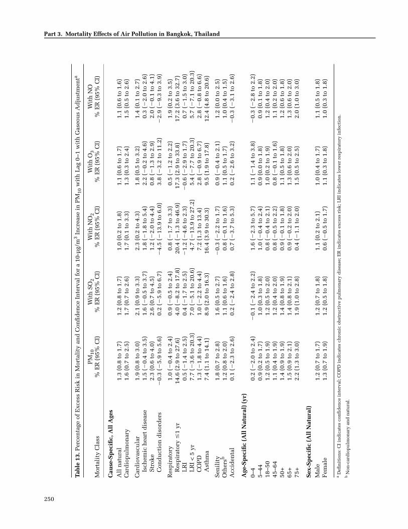
Table 12 presents the results for gaseous pollutants withPM10 included in the model. A lag 0–1 day was used for allpollutants. Not surprisingly, because of the high degree ofcorrelation among the pollutants, many of the effects ofgases were attenuated and often became insignificant afteradjusting for PM10. Of note, NO2 was no longer associatedwith any of the outcomes examined, except senility (which,as discussed earlier, may have been a misdiagnosis of car-diovascular disease). O3 remained associated with strokeand senility, and with those older than age 75, while NOremained associated with ischemic heart disease.

The results for PM10 with gaseous pollutants includedin the model are shown in Table 13. In this analysis, severalof the earlier associations remained, including effects on


‘

Table 10. Sensitivity Analyses: Natural Spline Models for Major Causes of Death with Different Degrees of Freedomfor Timea

Degrees of Freedom

PM10% ER (95% CI)

SO2% ER (95% CI)

NO2% ER (95% CI)

O3% ER (95% CI)

NO% ER (95% CI)

All Natural3 1.3 (0.9 to 1.8) 2.1 (0.6 to 3.6) 1.3 (0.8 to 1.8) 0.6 (0.3 to 0.9) 1.2 (0.7 to 1.7)4 1.2 (0.8 to 1.7) 1.4 (�0.1 to 2.9) 1.2 (0.7 to 1.7) 0.6 (0.3 to 0.9) 1.1 (0.6 to 1.6)6 1.3 (0.8 to 1.7) 1.6 (0.1 to 3.2) 1.4 (0.9 to 1.9) 0.6 (0.3 to 0.9) 1.1 (0.6 to 1.6)

9 1.1 (0.7 to 1.6) 2.2 (0.6 to 3.8) 1.3 (0.7 to 1.8) 0.6 (0.3 to 0.9) 1.0 (0.5 to 1.5)12 1.1 (0.6 to 1.5) 1.8 (0.2 to 3.4) 1.2 (0.6 to 1.7) 0.6 (0.2 to 0.9) 0.9 (0.4 to 1.4)15 1.2 (0.7 to 1.6) 1.5 (�0.2 to 3.2) 1.3 (0.7 to 1.8) 0.5 (0.2 to 0.9) 0.9 (0.4 to 1.5)

Cardiovascular3 2.0 (0.9 to 3.1) 1.6 (�2.1 to 5.4) 1.4 (0.2 to 2.7) 0.7 (0.0 to 1.5) 2.1 (0.9 to 3.3)4 1.9 (0.8 to 3.0) 0.8 (�2.8 to 4.7) 1.4 (0.2 to 2.7) 0.8 (0.0 to 1.5) 2.1 (0.9 to 3.3)6 1.9 (0.8 to 3.0) 0.8 (�3.0 to 4.7) 1.8 (0.5 to 3.1) 0.8 (0.0 to 1.7) 2.0 (0.7 to 3.2)

9 1.7 (0.6 to 2.8) 1.4 (�2.5 to 5.5) 1.7 (0.3 to 3.0) 0.7 (0.0 to 1.5) 2.0 (0.7 to 3.2)12 1.8 (0.7 to 3.0) 0.8 (�3.1 to 4.8) 1.5 (0.2 to 2.9) 0.8 (0.0 to 1.6) 1.7 (0.4 to 3.0)15 2.2 (0.9 to 3.4) 1.2 (�2.9 to 5.5) 2.0 (0.6 to 3.5) 1.0 (0.2 to 1.8) 1.9 (0.6 to 3.2)

Respiratory3 1.1 (�0.3 to 2.4) 2.5 (�2.2 to 7.3) 1.2 (�0.3 to 2.8) 0.9 (�0.1 to 1.9) �0.4 (�1.9 to 1.2)4 1.0 (�0.4 to 2.4) 1.3 (�3.3 to 6.2) 0.9 (�0.6 to 2.6) 0.9 (�0.1 to 1.9) �0.4 (�1.9 to 1.2)6 1.0 (�0.4 to 2.4) 1.7 (�3.1 to 6.6) 1.0 (�0.6 to 2.7) 0.9 (�0.1 to 1.9) �0.7 (�2.3 to 0.9)

9 0.7 (�0.7 to 2.1) 2.1 (�2.8 to 7.2) 0.7 (�1.0 to 2.4) 0.8 (�0.2 to 1.8) �0.9 (�2.5 to 0.7)12 0.3 (�1.1 to 1.8) 1.6 (�3.3 to 6.8) 0.5 (�1.2 to 2.2) 0.7 (�0.3 to 1.7) �1.3 (�2.8 to 0.3)15 0.3 (�1.1 to 1.9) 1.1 (�4.1 to 6.6) 0.6 (�1.1 to 2.4) 0.7 (�0.4 to 1.7) �1.3 (�2.9 to 0.3)

Age 65+b

3 1.6 (1.1 to 2.2) 3.4 (1.3 to 5.5) 1.5 (0.8 to 2.3) 0.7 (0.3 to 1.2) 1.5 (0.8 to 2.1)4 1.5 (0.9 to 2.1) 2.6 (0.5 to 4.7) 1.4 (0.7 to 2.1) 0.8 (0.3 to 1.2) 1.3 (0.6 to 2.0)6 1.5 (0.9 to 2.1) 2.8 (0.7 to 5.0) 1.8 (1.1 to 2.6) 0.8 (0.4 to 1.3) 1.3 (0.6 to 2.0)

9 1.4 (0.8 to 2.0) 3.9 (1.7 to 6.1) 1.7 (0.9 to 2.4) 0.9 (0.4 to 1.3) 1.2 (0.5 to 1.9)12 1.4 (0.8 to 2.0) 3.2 (1.1 to 5.5) 1.6 (0.8 to 2.3) 0.8 (0.4 to 1.3) 1.1 (0.4 to 1.8)15 1.5 (0.8 to 2.1) 3.0 (0.8 to 5.4) 1.7 (0.9 to 2.5) 0.8 (0.4 to 1.3) 1.1 (0.4 to 1.8)

a Definitions: CI indicates confidence interval; ER indicates excess risk. b For all natural mortality.

nonaccidental cardiopulmonary and asthma deaths, mor-tality among those older than age 65, and mortality amongmales and females. In addition, the effect estimatesremained relatively similar to those of the single-pollutantmodel for PM10.

Table 10 summarizes the results (for single-pollutantmodels) using different degrees of freedom in the specifi-cation of time in natural spline models. Specifically, weassessed the results of the models with 3 to 15 df fortime per year, while keeping 3 df for temperature andRH for the entire study period. With the exception of re-spiratory mortality, the results for PM10, SO2, NO2, O3, and

NO were robust to the degrees of freedom used in themodels, as the ER was generally similar. For respiratorymortality, increases in the degrees of freedom to 12 or moreper year significantly attenuated the effect estimate, exceptfor O3. Respiratory mortality effect estimates for this pol-lutant were robust to the degrees of freedom used to con-trol for time.

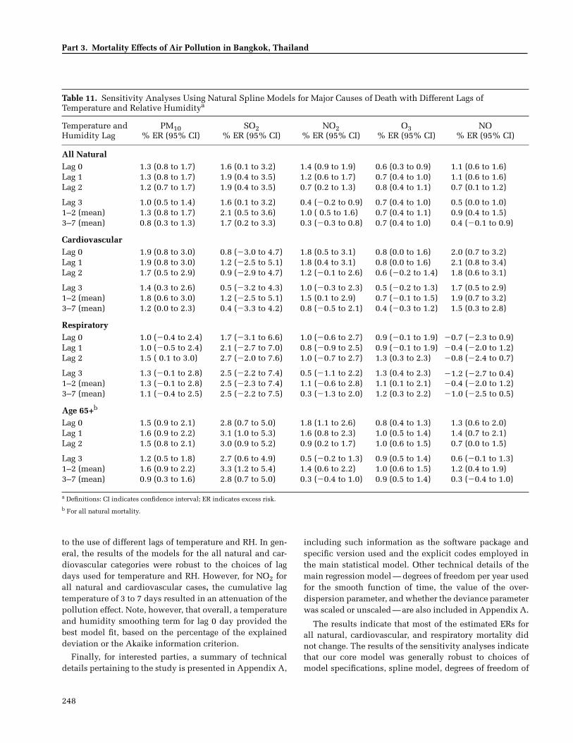
Next, we examined the results of the models with al-ternative lags for temperature and humidity, includingsingle-day lags of 0 to 3 days and cumulative lags of 1 to 2and 3 to 7 days. As shown in Table 11, we observed that forrespiratory mortality, the air pollutant effects were robust

247


Table 11. Sensitivity Analyses Using Natural Spline Models for Major Causes of Death with Different Lags of Temperature and Relative Humiditya

Temperature andHumidity Lag

PM10% ER (95% CI)

SO2% ER (95% CI)

NO2% ER (95% CI)

O3% ER (95% CI)

NO% ER (95% CI)

All NaturalLag 0 1.3 (0.8 to 1.7) 1.6 (0.1 to 3.2) 1.4 (0.9 to 1.9) 0.6 (0.3 to 0.9) 1.1 (0.6 to 1.6)Lag 1 1.3 (0.8 to 1.7) 1.9 (0.4 to 3.5) 1.2 (0.6 to 1.7) 0.7 (0.4 to 1.0) 1.1 (0.6 to 1.6)Lag 2 1.2 (0.7 to 1.7) 1.9 (0.4 to 3.5) 0.7 (0.2 to 1.3) 0.8 (0.4 to 1.1) 0.7 (0.1 to 1.2)

Lag 3 1.0 (0.5 to 1.4) 1.6 (0.1 to 3.2) 0.4 (�0.2 to 0.9) 0.7 (0.4 to 1.0) 0.5 (0.0 to 1.0)1–2 (mean) 1.3 (0.8 to 1.7) 2.1 (0.5 to 3.6) 1.0 ( 0.5 to 1.6) 0.7 (0.4 to 1.1) 0.9 (0.4 to 1.5)3–7 (mean) 0.8 (0.3 to 1.3) 1.7 (0.2 to 3.3) 0.3 (�0.3 to 0.8) 0.7 (0.4 to 1.0) 0.4 (�0.1 to 0.9)

CardiovascularLag 0 1.9 (0.8 to 3.0) 0.8 (�3.0 to 4.7) 1.8 (0.5 to 3.1) 0.8 (0.0 to 1.6) 2.0 (0.7 to 3.2)Lag 1 1.9 (0.8 to 3.0) 1.2 (�2.5 to 5.1) 1.8 (0.4 to 3.1) 0.8 (0.0 to 1.6) 2.1 (0.8 to 3.4)Lag 2 1.7 (0.5 to 2.9) 0.9 (�2.9 to 4.7) 1.2 (�0.1 to 2.6) 0.6 (�0.2 to 1.4) 1.8 (0.6 to 3.1)

Lag 3 1.4 (0.3 to 2.6) 0.5 (�3.2 to 4.3) 1.0 (�0.3 to 2.3) 0.5 (�0.2 to 1.3) 1.7 (0.5 to 2.9)1–2 (mean) 1.8 (0.6 to 3.0) 1.2 (�2.5 to 5.1) 1.5 (0.1 to 2.9) 0.7 (�0.1 to 1.5) 1.9 (0.7 to 3.2)3–7 (mean) 1.2 (0.0 to 2.3) 0.4 (�3.3 to 4.2) 0.8 (�0.5 to 2.1) 0.4 (�0.3 to 1.2) 1.5 (0.3 to 2.8)

RespiratoryLag 0 1.0 (�0.4 to 2.4) 1.7 (�3.1 to 6.6) 1.0 (�0.6 to 2.7) 0.9 (�0.1 to 1.9) �0.7 (�2.3 to 0.9)Lag 1 1.0 (�0.5 to 2.4) 2.1 (�2.7 to 7.0) 0.8 (�0.9 to 2.5) 0.9 (�0.1 to 1.9) �0.4 (�2.0 to 1.2)Lag 2 1.5 ( 0.1 to 3.0) 2.7 (�2.0 to 7.6) 1.0 (�0.7 to 2.7) 1.3 (0.3 to 2.3) �0.8 (�2.4 to 0.7)

Lag 3 1.3 (�0.1 to 2.8) 2.5 (�2.2 to 7.4) 0.5 (�1.1 to 2.2) 1.3 (0.4 to 2.3) �1.2 (�2.7 to 0.4)1–2 (mean) 1.3 (�0.1 to 2.8) 2.5 (�2.3 to 7.4) 1.1 (�0.6 to 2.8) 1.1 (0.1 to 2.1) �0.4 (�2.0 to 1.2)3–7 (mean) 1.1 (�0.4 to 2.5) 2.5 (�2.2 to 7.5) 0.3 (�1.3 to 2.0) 1.2 (0.3 to 2.2) �1.0 (�2.5 to 0.5)

Age 65+b

Lag 0 1.5 (0.9 to 2.1) 2.8 (0.7 to 5.0) 1.8 (1.1 to 2.6) 0.8 (0.4 to 1.3) 1.3 (0.6 to 2.0)Lag 1 1.6 (0.9 to 2.2) 3.1 (1.0 to 5.3) 1.6 (0.8 to 2.3) 1.0 (0.5 to 1.4) 1.4 (0.7 to 2.1)Lag 2 1.5 (0.8 to 2.1) 3.0 (0.9 to 5.2) 0.9 (0.2 to 1.7) 1.0 (0.6 to 1.5) 0.7 (0.0 to 1.5)

Lag 3 1.2 (0.5 to 1.8) 2.7 (0.6 to 4.9) 0.5 (�0.2 to 1.3) 0.9 (0.5 to 1.4) 0.6 (�0.1 to 1.3)1–2 (mean) 1.6 (0.9 to 2.2) 3.3 (1.2 to 5.4) 1.4 (0.6 to 2.2) 1.0 (0.6 to 1.5) 1.2 (0.4 to 1.9)3–7 (mean) 0.9 (0.3 to 1.6) 2.8 (0.7 to 5.0) 0.3 (�0.4 to 1.0) 0.9 (0.5 to 1.4) 0.3 (�0.4 to 1.0)

a Definitions: CI indicates confidence interval; ER indicates excess risk.b For all natural mortality.

to the use of different lags of temperature and RH. In gen-eral, the results of the models for the all natural and car-diovascular categories were robust to the choices of lagdays used for temperature and RH. However, for NO2 forall natural and cardiovascular cases, the cumulative lagtemperature of 3 to 7 days resulted in an attenuation of thepollution effect. Note, however, that overall, a temperatureand humidity smoothing term for lag 0 day provided thebest model fit, based on the percentage of the explaineddeviation or the Akaike information criterion.

Finally, for interested parties, a summary of technicaldetails pertaining to the study is presented in Appendix A,

248

including such information as the software package andspecific version used and the explicit codes employed inthe main statistical model. Other technical details of themain regression model — degrees of freedom per year usedfor the smooth function of time, the value of the over-dispersion parameter, and whether the deviance parameterwas scaled or unscaled — are also included in Appendix A.

The results indicate that most of the estimated ERs forall natural, cardiovascular, and respiratory mortality didnot change. The results of the sensitivity analyses indicatethat our core model was generally robust to choices ofmodel specifications, spline model, degrees of freedom of


Table 12. Percentage of Excess Risk in Mortality and Confidence Interval for a 10-µg/m3 Increase in Gases with Lag 0–1 with PM10 Adjustmenta

Mortality Class SO2 % ER (95% CI)

NO2% ER (95% CI)

O3% ER (95% CI)

NO% ER (95% CI)

Cause-Specific, All AgesAll natural 0.1 (�1.5 to 1.7) 0.4 (�0.5 to 1.4) 0.2 (�0.2 to 0.5) 0.4 (�0.2 to 1.0)Cardiopulmonary �1.0 (�4.2 to 2.3) �0.2 (�2.1 to 1.7) 0.3 (�0.5 to 1.1) 0.1 (�1.1 to 1.2)

Cardiovascular �2.0 (�6.0 to 2.1) �0.5 (�2.9 to 1.9) 0.1 (�0.9 to 1.0) 1.1 (�0.3 to 2.6)Ischemic heart disease �0.8 (�7.9 to 6.8) �0.4 (�4.5 to 3.9) �0.9 (�2.5 to 0.8) 2.6 (0.0 to 5.2)Stroke �2.6 (�8.9 to 4.1) 1.6 (�2.2 to 5.5) 1.9 (0.4 to 3.5) 0.6 (�1.6 to 3.0)Conduction disorders �4.4 (�24.0 to 20.4) 6.3 (�6.1 to 20.3) �5.0 (�9.7 to 0.0) 6.0 (�1.9 to 14.5)

Respiratory 0.7 (�4.4 to 6.0) 0.3 (�2.7 to 3.4) 0.7 (�0.5 to 1.9) �1.8 (�3.6 to 0.0)Respiratory � 1 yr 98.8 (26.0 to 213.8) �6.5 (�25.5 to 17.3) �2.8 (�11.2 to 6.5) �4.8 (�16.8 to 9.0)LRI 1.5 (�5.6 to 9.1) 1.9 (�1.7 to 5.7) 1.4 (�0.2 to 3.1) �0.3 (�2.8 to 2.2)LRI < 5 yr 6.3 (�31.0 to 63.8) 4.1 (�17.2 to 31.0) 2.8 (�6.4 to 12.9) 4.0 (�9.8 to 19.9)COPD 2.7 (�7.9 to 14.6) �7.9 (�14.0 to �1.3) �1.9 (�4.6 to 0.8) �3.2 (�7.1 to 0.9)Asthma �12.1 (�30.7 to 11.5) �11.0 (�22.5 to 2.3) �2.6 (�7.8 to 2.9) �9.5 (�16.8 to �1.7)

Senility 1.5 (�2.3 to 5.5) 3.0 (0.6 to 5.5) 1.2 (0.3 to 2.2) 1.1 (�0.3 to 2.6)Othersb 0.4 (�1.4 to 2.2) 0.6 (�0.5 to 1.7) 0.1 (�0.3 to 0.5) 0.5 (�0.2 to 1.1)Accidental �0.2 (�8.7 to 9.2) �0.8 (�6.0 to 4.8) �0.1 (�2.2 to 2.1) 0.9 (�2.3 to 4.2)

Age-Specific (All Natural) (yr)0–4 3.4 (�4.5 to 12.0) �2.1 (�6.7 to 2.8) �1.3 (�3.1 to 0.6) 1.1 (�1.8 to 4.2)5–44 �1.0 (�3.7 to 1.8) �0.1 (�1.7 to 1.6) 0.0 (�0.6 to 0.7) 0.0 (�1.0 to 1.0)18–50 �0.6 (�3.0 to 2.0) 0.5 (�1.0 to 2.0) 0.2 (�0.4 to 0.8) �0.1 (�1.0 to 0.9)45–64 �0.6 (�3.4 to 2.2) 0.5 (�1.2 to 2.1) 0.5 (�0.1 to 1.2) 0.1 (�0.9 to 1.1)50+ 0.7 (�1.2 to 2.6) 0.8 (�0.3 to 2.0) 0.4 (�0.1 to 0.8) 0.5 (�0.2 to 1.2)65+ 1.1 (�1.1 to 3.4) 0.9 (�0.4 to 2.3) 0.3 (�0.2 to 0.8) 0.5 (�0.3 to 1.3)75+ 2.4 (�0.8 to 5.6) 2.5 (0.6 to 4.5) 0.9 (0.1 to 1.6) 0.4 (�0.7 to 1.6)

Sex-Specific (All Natural)Male �0.7 (�2.6 to 1.3) 0.0 (�1.1 to 1.2) 0.2 (�0.3 to 0.6) 0.1 (�0.6 to 0.8)Female 1.1 (�1.1 to 3.5) 1.0 (�0.4 to 2.4) 0.3 (�0.3 to 0.8) 0.6 (�0.3 to 1.4)

a Definitions: CI indicates confidence interval; COPD indicates chronic obstructive pulmonary disease; ER indicates excess risk; LRI indicates lower respiratory infection.

b Non-cardiopulmonary and natural.

time-smoothing functions, lags for temperature, adjust-ment for autocorrelation, adjustment for influenza epidem-ics, and adjustment for missing values using centered data.

In our final analysis of the effects of pollution on mortal-ity, we examined the shape of the concentration–responsefunction. All of our previous analyses (and those of mostother previous studies) assumed linear models of expo-sure to PM10, SO2, NO2, O3, and NO. We investigated thepossibility of nonlinear functions given the relatively highconcentrations of pollution observed in the PAPA cities.This is important since it is likely that at some high con-centrations, the concentration–response function will tendto level off. To assess this question, we examined thesmoothed relation between pollution and mortality, after

controlling for other factors in the analysis. Again, we useda lag 0–1 day for pollutants. Residuals of mortality —variations of daily mortality obtained after adjusting fortime and weather — were created after fitting our coremodel, omitting the pollution term. As shown in Figure 6,the concentration–response relation between each air pol-lutant and all natural mortality appears to be fairly linear,except for NO2, which appears to show an increasing effectat higher concentrations, based on a limited number ofobservations at the higher levels. We conducted a specifictest for linearity (see Appendix A), which was rejected onlyfor NO2. The findings indicated that our models were rea-sonably appropriate for assessing the effects of air pollut-ants on mortality.

249

250


Tabl

e 13

. Per

cen

tage

of

Exc

ess

Ris

k in

Mor

tali

ty a

nd

Con

fid

ence

In

terv

al f

or a

10-

µg/

m3

Incr

ease

in

PM

10 w

ith

Lag

0–1

wit

h G

aseo

us

Ad

just

men

ta

Mor

tali

ty C

lass

PM

10%

ER

(95

% C

I)W

ith

SO

2%

ER

(95

% C

I)W

ith

NO

2%

ER

(95

% C

I)W

ith

O3

% E

R (

95%

CI)

Wit

h N

O%

ER

(95

% C

I)

Cau

se-S

pec

ific,

All

Age

sA

ll n

atu

ral

1.3

(0.8

to

1.7)

1.2

(0.8

to

1.7)

1.0

(0.2

to

1.8)

1.1

(0.6

to

1.7)

1.1

(0.6

to

1.6)

Car

dio

pu

lmon

ary

1.6

(0.7

to

2.5)

1.7

(0.7

to

2.6)

1.7

(0.1

to

3.3)

1.3

(0.3

to

2.4)

1.5

(0.5

to

2.6)

Car

dio

vasc

ula

r1.

9 (0

.8 t

o 3.

0)2.

1 (0

.9 t

o 3.

3)2.

3 (0

.2 t

o 4.

3)1.

8 (0

.5 t

o 3.

2)1.

4 (0

.1 t

o 2.

7)Is

chem

ic h

eart

dis

ease

1.5

(�0.

4 to

3.5

)1.

6 (�

0.5

to 3

.7)

1.8

(�1.

8 to

5.4

)2.

2 (�

0.2

to 4

.6)

0.3

(�2.

0 to

2.6

)S

trok

e2.

3 (0

.6 t

o 4.

0)2.

6 (0

.7 t

o 4.

5)1.

2 (�

2.0

to 4

.4)

0.8

(�1.

3 to

2.9

)2.

0 (�

0.1

to 4

.1)

Con

du

ctio

n d

isor

der

s�

0.3

(�5.

9 to

5.6

)0.

2 (�

5.9

to 6

.7)

�4.

5 (�

13.9

to

6.0)

3.8

(�3.

2 to

11.

2)�

2.9

(�9.

3 to

3.9

)

Res

pir

ator

y1.

0 (�

0.4

to 2

.4)

0.9

(�0.

5 to

2.4

)0.

8 (�

1.7

to 3

.3)

0.5

(�1.

2 to

2.2

)1.

9 (0

.2 t

o 3.

5)R

esp

irat

ory

�1

yr14

.6 (

2.9

to 2

7.6)

4.0

(�8.

2 to

17.

8)20

.4 (

�1.

3 to

46.

9)17

.3 (

2.9

to 3

3.8)

17.2

(3.

6 to

32.

7)L

RI

0.5

(�1.

4 to

2.5

)0.

4 (�

1.7

to 2

.5)

�1.

2 (�

4.6

to 2

.3)

�0.

6 (�

2.9

to 1

.7)

0.7

(�1.

5 to

3.0

)L

RI

< 5

yr

7.7

(�3.

6 to

20.

3)7.

0 (�

5.1

to 2

0.6)

4.7

(�13

.9 t

o 27

.2)

5.4

(�7.

7 to

20.

3)5.

7 (�

7.1

to 2

0.3)

CO

PD

1.3

(�1.

8 to

4.4

)1.

0 (�

2.2

to 4

.4)

7.2

(1.3

to

13.4

)2.

8 (�

0.9

to 6

.7)

2.8

(�0.

8 to

6.6

)A

sth

ma

7.4

(1.1

to

14.1

)8.

9 (2

.0 t

o 16

.3)

16.4

(3.

9 to

30.

3)9.

5 (1

.9 t

o 17

.8)

12.4

(4.

8 to

20.

6)

Sen

ilit

y1.

8 (0

.7 t

o 2.

8)1.

6 (0

.5 t

o 2.

7)�

0.3

(�2.

2 to

1.7

)0.

9 (�

0.4

to 2

.1)

1.2

(0.0

to

2.5)

Oth

ersb

1.2

(0.8

to

2.0)

1.1

(0.6

to

1.6)

0.8

(�0.

1 to

1.6

)1.

1 (0

.5 t

o 1.

7)1.

0 (0

.4 t

o 1.

5)A

ccid

enta

l0.

1 (�

2.3

to 2

.6)

0.2

(�2.

4 to

2.8

)0.

7 (�

3.7

to 5

.3)

0.2

(�2.

6 to

3.2

)�

0.3

(�3.

1 to

2.6

)

Age

-Sp

ecifi

c (A

ll N

atu

ral)

(yr

)0–

40.

2 (�

2.0

to 2

.4)

�0.

1 (�

2.4

to 2

.2)

1.6

(�2.

3 to

5.7

)1.

1 (�

1.4

to 3

.8)

�0.

3 (�

2.8

to 2

.2)

5–44

0.9

(0.2

to

1.7)

1.0

(0.3

to

1.8)

1.0

(�0.

4 to

2.4

)0.

9 (0

.0 t

o 1.

8)0.

9 (0

.1 t

o 1.

8)18

–50

1.2

(0.5

to

1.9)

1.2

(0.5

to

2.0)

0.8

(�0.

4 to

2.1

)1.

0 (0

.2 t

o 1.

9)1.

2 (0

.4 t

o 2.

0)45

–64

1.1

(0.4

to

1.9)

1.2

(0.4

to

2.0)

0.8

(�0.

5 to

2.2

)0.

8 (�

0.1

to 1

.6)

1.1

(0.2

to

2.0)

50+

1.4

(0.9

to

1.9)

1.4

(0.8

to

1.9)

0.9

(�0.

1 to

1.8

)1.

1 (0

.5 t

o 1.

8)1.

2 (0

.6 t

o 1.

8)65

+1.

5 (0

.9 t

o 2.

1)1.

4 (0

.8 t

o 2.

1)0.

9 (�

0.2

to 2

.0)

1.3

(0.6

to

2.0)

1.3

(0.6

to

2.0)

75+

2.2

(1.3

to

3.0)

1.9

(1.0

to

2.8)

0.4

(�1.

1 to

2.0

)1.

5 (0

.5 t

o 2.

5)2.

0 (1

.0 t

o 3.

0)

Sex

-Sp

ecifi

c (A

ll N

atu

ral)

Mal

e1.

2 (0

.7 t

o 1.

7)1.

2 (0

.7 t

o 1.

8)1.

1 (0

.2 t

o 2.

1)1.

0 (0

.4 t

o 1.

7)1.

1 (0

.5 t

o 1.

8)F

emal

e1.

3 (0

.7 t

o 1.

9)1.

2 (0

.5 t

o 1.

8)0.

6 (�

0.5

to 1

.7)

1.1

(0.3

to

1.8)

1.0

(0.3

to

1.8)

a D

efin

itio

ns:

CI

ind

icat

es c

onfi

den

ce i

nte

rval

; CO

PD

in

dic

ates

ch

ron

ic o

bstr

uct

ive

pu

lmon

ary

dis

ease

; ER

in

dic

ates

exc

ess

risk

; LR

I in

dic

ates

low

er r

esp

irat

ory

infe

ctio

n.

b N

on-c

ard

iop

ulm

onar

y an

d n

atu

ral.


Figure 6. Curves showing the concentration–response relation between air pollutants and all natural mortality. Small bar graphs along the x-axes showareas of sparse data; there were many fewer days with high concentrations of air pollutants as shown by wide spacing between bars.

DISCUSSION

The results of our analysis of five years of data fromBangkok, Thailand, indicate a statistically significant asso-ciation between daily mortality and daily concentrationsof PM10, NO2, NO, and O3. More modest associations werefound with SO2. For PM10, the effect estimates for allnatural mortality, cardiovascular-related and respiratory-related mortality, and mortality among those over age65 years are generally similar to those found in other stud-ies, although high in that range (U.S. EPA 2004). A 10-µg/m3

change in PM10 was associated with an ER of death of1.3%, 1.9%, 1.0%, and 1.5% in the categories of all natu-ral, cardiovascular-related, and respiratory-related deaths,and among those over age 65, respectively (Table 7a). TheCI for respiratory mortality included zero, however (indi-cating nonsignificant association). These estimates are gen-erally similar to those reported by Ostro and colleagues(1998, 1999) and Vajanapoom and associates (2002) in pre-vious studies in Bangkok covering earlier years. However,

these older studies largely utilized PM10 data from airportvisibility measurements rather than direct measurementsof PM10. Nevertheless, these previous results are supportedby the current analysis, which used mortality and air pol-lution data that was subjected to significant quality assur-ance and quality control procedures. As such, they mayrank among the highest quality and most complete mortal-ity and pollution data from less-developed countries.

Our results also found some disease- and age-specificsubgroups that exhibit ERs of death. ERs from PM10 wereobserved for many of the cardiovascular- and respiratory-disease subclasses of mortality, with particularly high risksrelated to respiratory diseases in those less than 1 year ofage, LRI for those under 5 years, asthma, stroke, and senil-ity, although many of the deaths attributed to senility mayhave actually been misclassified cardiovascular mortalities.Analysis by age indicated associations with PM10 for all ofthe subgroups with the exception of those under age 5. Forthat group, no associations were observed for all naturalmortality, although, as indicated earlier, associations were

251


observed for that group for respiratory mortality. Our exam-ination of lags indicated that among single-day lags, a zero-or one-day lag (lag 0 day or lag 1 day, respectively) wasimportant, but that multiday averages of 5 days generatedthe largest effect estimates. We did not find associationswith COPD, possibly due to low daily death counts (about2 per day) or misclassification of diseases. It should be notedthat the daily counts for some of the outcomes, such asasthma-related and infant-respiratory-related mortality, werelow, so caution is suggested in interpreting these results.

Many of the PM10 associations with mortality wereretained in multipollutant models. However, notably therewas a high correlation between PM10 and several of theother pollutants, particularly NO2 (r = 0.71). This makes itdifficult to separate out the independent effects of PM10from those of NO2 and leads to an attenuation of the pollu-tion effect when both of these pollutants are included inthe same model. Associations between the other pollut-ants (SO2, NO2, NO, and O3) and mortality were oftenobserved in single-pollutant models. However, the effectswere greatly attenuated and often insignificant when PM10was also included in the model. Since air pollution inBangkok is dominated by traffic, it is not surprising thatPM10 would be highly correlated with traffic-based pollut-ants such as NO2 and NO. Of particular note is the poten-tial independent effect of O3. For example, while most ofthe pollutants exhibited larger effects for cardiovascularmortality, O3 had larger effects on respiratory mortality(Table 7a). In contrast, SO2, NO2, and NO were not associ-ated with respiratory mortality. In addition, in models thatincluded PM10, O3 remained associated with stroke andwith deaths among those over the age of 75 (Table 12),and NO2 was associated only with deaths among thoseover the age of 75, whereas those results were not observedfor SO2 or NO. These findings suggest a plausible indepen-dent effect of O3.

We conducted extensive sensitivity analyses to investi-gate whether the results were robust to various assump-tions. The results indicated that most of the estimated ERsfor all natural, cardiovascular-related, and respiratory-related mortality were not sensitive to our core modelingassumptions. Specifically, the results of our core modelswere not significantly affected by the choice of model spec-ifications, spline model (natural versus penalized), degreesof freedom of time smoothing (from 3 to 15 df), lags fortemperature (zero- to 3-day), adjustment for autocorrela-tion, adjustment for epidemics, and adjustment for miss-ing values using centered data. Of note, however, is thatwhen longer cumulative lags of temperature were used(lags of 3 to 7 days), the effect estimates for PM10 were sig-nificantly reduced. However, the best overall model fit wasobserved for a lag 0 day for temperature. Therefore, it is

252

most likely that the attenuation of the pollution effect with alonger cumulative lag in temperature (specifically, the meanof temperature from lag 3–7 days) was due to its correlationwith lags in pollution (see Tables B.4–B.8 in Appendix B)coupled with the greater effect of cumulative averages (rel-ative to single-day averages) of PM10 on mortality. Finally,our analysis showed a fairly linear concentration–responserelation between each air pollutant (except for NO2) andall natural mortality (Figure 6).

Generally, our analysis of short-term changes in dailymortality per 10-µg/m3 increase in PM10 in Bangkok gener-ated effect estimates that are higher than most previouslyreported. For example, our estimate for all natural mor-tality is 1.3% (95% CI, 0.8 to 1.7). As a comparison, ananalysis of 75 single-city time-series analyses generated anestimate of 0.6% (95% CI, 0.5 to 0.7) (Anderson et al.2005). A study of the 90 largest cities in the United Statesgave an estimate of 0.2% (95% CI, 0.1 to 0.4) (Dominici etal. 2003), while a study of 29 European cities provided anestimate of 0.6% (95% CI, 0.4 to 0.7) (Katsouyanni et al.2003). A study of 14 cities in the United States using acase-crossover approach generated an estimate of 0.35%(95% CI, 0.2 to 0.5) (Schwartz 2004). A meta-analysis ofAsian studies using a random-effects estimate gave an esti-mate of 0.49% (95% CI, 0.23 to 0.76) based on four cities:Bangkok, Seoul, Inchon, and Hong Kong (HEI Interna-tional Scientific Oversight Committee 2004). Thus, it isclear that the results for Bangkok are at the upper end ofthe range of estimates. It is also of note that some high esti-mates have been reported in other developing countries.For example, a study in Mexico City reported an ER of1.8% (95% CI, 0.9 to 2.7), while an analysis of Santiago,Chile, generated an ER of 1.1% (95% CI, 0.9 to 1.4) (Ostroet al. 1996; Castillejos et al. 2000).

We can speculate on several possible reasons for thefinding of high effect estimates in Bangkok relative to mostother cities, including (1) differences in particle chemistryin Bangkok; (2) the proximity of a large portion of the pop-ulation to roads and traffic congestion; (3) the likely highpenetration rates due to the low prevalence of air condition-ing and the presence of open ventilation between indoorsand outdoors; (4) the greater duration of exposure due to theamount of time spent outdoors; (5) factors related to lowereconomic development and socioeconomic status, such asbackground health status, use of health care, smoking rates,and comorbidity; and (6) stochastic variability. Several ofthese factors (although only anecdotal in nature) may ex-plain why the effective exposure to any given concentrationmeasured from a fixed-site outdoor monitor is also greaterthan that observed in the Western industrialized countries.Although there is limited empiric evidence about these fac-tors, one study in Bangkok demonstrated high correlations


between outdoor and indoor PM10 and PM2.5 (particulatematter � 2.5 µm in aerodynamic diameter), particularly inhomes with limited indoor sources (Tsai et al. 2000).

Most previous studies of air pollution and mortality havebeen conducted in cities in the United States and WesternEurope — areas with relatively cold winters and strong sea-sonal patterns in daily mortality. Our replication of previ-ous time-series studies showing associations between PM10and mortality in a city with a very different seasonal pattern,and no cold season, is notable. Specifically, we have foundan association between mortality and air pollution in a lo-cation where there is very little likelihood of confoundingdue to seasonality or epidemics related to cold weather.

For the most part, policy makers in Asia have had to drawfrom studies that have been conducted in North Americaand Western Europe. For example, the WHO effort to esti-mate the global burden of disease from outdoor air pollu-tion relied primarily on studies conducted in the Western,industrialized nations (Cohen et al. 2005). Similarly, pre-vious guidance from WHO (Ostro 2004) and the WorldBank (Ostro 1994) for developing estimates of the healtheffects of air pollution in developing countries also fo-cused largely on studies from the industrialized West. Thecurrent study suggests that it is reasonable to extrapolatethe findings from the North American and Western Euro-pean regions to other parts of the world. However, ourstudy also suggests the possibility that the per-unit effectsmay be higher in certain developing countries. Additionalstudies undertaken in developing countries in Asia andother parts of the world may serve to validate our find-ings and help determine the factors that might modify theeffect estimate.

To date, studies of daily mortality in Asia have beenconducted in Inchon, Korea (Hong et al. 1999); Seoul andUlsan, Korea (Lee et al. 1999; Lee and Schwartz 1999;Kwon et al. 2001); Shenyang, China (Xu et al. 2000); sevencities in South Korea (Lee et al. 2000); and New Delhi,India (Cropper et al. 1997). These studies generally reportassociations consistent with those found in studies under-taken in Western, industrialized nations. To further exam-ine this issue, HEI has provided support for an analysis ofthree Chinese cities as part of the PAPA project — HongKong, Shanghai, and Wuhan — in addition to Bangkok.

Given the relatively few studies conducted to date in de-veloping countries in Asia, particularly for mortality, ourfindings for Bangkok lend critical support to the extrapola-tion of empirical findings from Western, industrializednations. Therefore, the exposure of hundreds of millions ofpeople in Asia to high concentrations of PM10 and otherambient air pollutants most likely represents a significantand preventable public health burden.

ACKNOWLEDGMENTS

This study would not have been possible without con-tributions from and the support of many people. We wishto thank the staff at the Thailand Ministry of Public Health,the Pollution Control Department of the Thailand Ministryof Natural Resources and Environment, and the ThailandMeteorological Department, who provided us with thecore data for our study. We also appreciate their patiencein answering our questions and meeting our requests. Aspecial thanks goes to Dr. Supat Wangwongwatana, DeputyDirector of the Pollution Control Department, who pro-vided us with easy and timely access to air quality data.

We were quite fortunate to be surrounded by those whoprovided us with valuable comments and suggestions.Much of the improvement of our study can be attributed totheir advice. One such group of mentors was the Interna-tional Scientific Oversight Committee. Their feedback onall our progress reports and workshops contributed to thedepth and comprehensiveness of our approach and analy-sis. Additionally, our thanks go to Kristin Hoover, LindaCalisti, and Warren White, who taught us that data audit-ing is not just a scrutinizing process, in which detection oferror is the only objective, but also a way to review andrevisit data in order to be confident of their quality. Theirsuggestions and advice exceeded our expectations. Theirrelaxed and affable attitudes reassured us that auditingcould be a learning experience.

We wish to extend our sincere appreciation to Dr. WeiHuang and Dr. Sumi Mehta for their earnest guidance andefforts in keeping us on track, both administratively andacademically, throughout the two years. We wish to thankthem for being our friends. Also, our study would nothave run smoothly without administrative assistance fromJacqueline Rutledge and Francine Marmenout, as well asother HEI staff members.

We have gained much more than just scientific knowledgefrom this study from working closely with our colleaguesin the PAPA project. The friendship and bonds that havedeveloped are valuable by-products that extend beyondthis project. We had the opportunity to come to know ourcolleagues, not only as professionals, but also as peoplewho have many facets to their lives.

None of this would have been possible without HEI’ssupport from the beginning to the end. We truly appreciateDaniel Greenbaum and Robert O’Keefe for including us inthis important endeavor. Their commitment to, support of,and confidence in the PAPA project and the researchersinvolved greatly contributed to its success. We are thankfulfor the opportunity to be a part of this important researchlandmark in environmental epidemiology in Asia.

253


REFERENCES

Anderson HR, Atkinson RW, Peacock JL, Sweeting MJ,Marston L. 2005. Ambient particulate matter and healtheffects: Publication bias in studies of short-term associa-tions. Epidemiol 16:155–163.

Anderson HR, Atkinson RW, Peacock JL, Marston L,Konstantinou K. 2004. Meta-analysis of time-series studiesand panel studies of particulate matter (PM) and ozone(O3): Report of a WHO task group. http://www.euro.who.int/document/e82792.pdf

Bangkok Metropolitan Administration. 2003. Populationand household statistics in Bangkok by sub-district anddistricts in December 2003. www.bma.go.th/info/. Accessed10/9/2003.

Castillejos M, Borja-Aburto VH, Dockery DW, Gold DR,Loomis D. 2000. Airborne coarse particles and mortality.In: Inhalation Toxicology: Proceedings of the Third Collo-quium on Particulate Air Pollution and Human Health(first special issue) June 1999 (Phalen RF, ed.). Durham,NC. Inhal Toxicol 12(S1):61–72.

Cohen AJ, Anderson RH, Ostro B, Pandey KD, Krzyza-nowski M, Kunzli N, Gutschmidt K, Pope A, Romieu I,Samet JM, Smith K. 2005. The global burden of disease dueto outdoor air pollution. J Toxicol Environ Health A 68:1301–1307.

Cropper ML, Simon NB, Alberini A, Arora S, Sharma PK.1997. The health benefits of air pollution control in Delhi.Am J Agric Econ 79:1625–1629.

Dominici F, McDermott A, Daniels M, Zeger SL, Samet JM.2003. Mortality among residents of 90 cities. In: RevisedAnalyses of Time-Series Studies of Air Pollution and Health.Special Report. Health Effects Institute, Boston MA.

Health Effects Institute. 2003. Revised Analysis of Time-Series Studies of Air Pollution and Health. Special Report.Health Effects Institute, Boston, MA.

HEI International Scientific Oversight Committee. 2004.Health Effects of Outdoor Air Pollution in DevelopingCountries of Asia: A Literature Review. Special Report 15.Health Effects Institute, Boston, MA.

Hong YC, Leem JH, Ha EH, Christiani DC. 1999. PM10exposure, gaseous pollutants, and daily mortality in Inchon,South Korea. Environ Health Perspect 107:873–878.

Katsouyanni K, Touloumi G, Samolu E, Petasakis Y,Analitis A, Le Tertre A, Rossi G, Zmirou D, Ballester F,Boumghar A, Anderson HR, Wojtyniak B, Paldy A,

254

Braustein R, Pekkanen J, Schindler C, Schwartz J. 2003.Sensitivity analysis of various models of short-termeffects of ambient particles on total mortality in 29 citiesin APHEA2. In: Revised Analyses of Time-Series of AirPollution and Health. Special Report. Health Effects Insti-tute, Boston, MA.

Kwon HJ, Cho SH, Nyberg F, Pershagen G. 2001. Effects ofambient air pollution on daily mortality in a cohort ofpatients with congestive heart failure. Epidemiology12:413–419.

Lee JT, Kim H, Hong YC, Kwon HJ, Schwartz J, ChristianiDC. 2000. Air pollution and daily mortality in seven majorcities of Korea, 1991–1997. Environ Res 84:247–254.

Lee JT, Schwartz J. 1999. Reanalysis of the effects of air pol-lution on daily mortality in Seoul, Korea: A case-crossoverdesign. Environ Health Perspect 107:633–636.

Lee JT, Shin D, Chung Y. 1999. Air pollution and daily mor-tality in Seoul and Ulsan, Korea. Environ Health Perspect107:149–154.

Mikkelsen TN, Ro-Poulsen H, Pilegaard K, Hovmand MF,Jensen NO, Christensen CS, Hummelshoej P. 2000. Ozoneuptake by an evergreen forest canopy: Temporal variationand possible mechanisms. Environ Pollut 109:423–429.

Nair PR, Chand D, Lal S, Modh KS, Naja M, ParameswaranK, Ravindran S, Venkataramani S. 2002. Temporal varia-tions in surface ozone at Thumba (8.6�N, 77�E): A tropicalcoastal site in India. Atmos Environ 36:603–610.

Ostro B. 1994. Estimating the health effects of air pollution:A method with an application to Jakarta. Policy researchworking paper 1301. World Bank, Washington, DC.

Ostro B. 2004. Outdoor Air Pollution: Assessing the Envi-ronmental Burden of Disease at National and Local Levels.Environmental Burden of Disease Series, No. 5. WorldHealth Organization, Geneva, Switzerland.

Ostro B, Chestnut L, Vichit-Vadakan N, Laixuthai A.1998. The impact of fine particulate matter on mortality inBangkok, Thailand. In: PM2.5: A Fine Particle Standard,Volume II (Chow J, Koutrakis P, eds.). Air and Waste Man-agement Association, Pittsburgh, PA.

Ostro BD, Chestnut L, Vichit-Vadakan N, Laixuthai A.1999. The impact of particulate matter on daily mortality inBangkok, Thailand. J Air Waste Manag Assoc 49:100–107.

Ostro B, Sanchez JM, Aranda C, Eskeland GS. 1996. Airpollution and mortality: Results from a study of Santiago,Chile. J Expo Anal Environ Epidemiol 6:97–114.


Pollution Control Department (Thailand). 2007. Air Qualityand Noise Standards. www.pcd.go.th/info_serv/. Accessed12/5/2007.

Reddy RR, Gopal KR, Narasimhulu K, Reddy LSS, KumarKR, Ahammed YN, Rao TVR, Azeem PA. 2008. Diurnaland seasonal variabilities in surface ozone and its pre-cursor gases at a semi-arid site Anantapur (14.62� N, 77.65�

E, 331 m asl) in India. Internat J Environ Stud 65:247–265.

Schwartz J. 2004. The effects of particulate air pollution ondaily deaths: A multi-city case-crossover analysis. OccupEnviron Med 61:956–961.

Tao Z, Larson SM, Williams A, Caughey M, Wuebbles DJ.2004. Sensitivity of regional ozone concentrations to temporaldistribution of emissions. Atmos Environ 38:6279–6285.

Tsai FC, Smith KR, Vichit-Vadakan N, Ostro BD, ChestnutLG, Kungskulniti N. 2000. Indoor/outdoor PM10 and PM2.5in Bangkok, Thailand. J Exp Anal Environ Epidemiol 10:15–26.

U.S. Environmental Protection Agency. 2004. Review ofthe National Ambient Air Quality Standards for Particu-late Matter. EPA-452/R-96-013. Office of Air Quality Plan-ning and Standards, Research Triangle Park, NC.

U.S. Environmental Protection Agency. 2007. National Am-bient Air Quality Standards (NAAQS). www.epa.gov/air.Accessed 12/5/2007.

Vajanapoom N, Shy C, Neas L, Loomis D. 2002. Associationsof particulate matter and daily mortality in Bangkok, Thai-land. Southeast Asian J Trop Med Public Health 33: 389–399.

Wong CM, Ma S, Hedley AJ, Lam TH. 2001. Effect of airpollution on daily mortality in Hong Kong. Environ HealthPerspect 109:335–340.

World Health Organization. 2000. WHO Air Quality Guide-lines for Europe. European Series, No. 91. 2nd edition. WHORegional Office for Europe, WHO Regional Publications,Copenhagen, Denmark.

Xu Z, Yu D, Jing L, Xu X. 2000. Air pollution and daily mor-tality in Shenyang, China. Arch Environ Health 55: 115–120.

APPENDIX A. Technical Summary

STATISTICAL METHODS

To assess the short-term effects of PM10 and gaseous pol-lutants on daily mortality, we followed the Common Pro-tocol of the PAPA project (found at the end of this volume).In all analyses, we used natural cubic spline models using

the statistical software package R, version 2.5, with mgcv,version 1.3–24 (R Development Core Team 2007, Vienna,Austria). We used the quasi-Poisson structure in the gener-alized additive model option. This method accounts for theoverdispersion in the confidence intervals and P values.The general form of the model is as follows:

Where E[Yt] = expected count of the health outcome onday t; �1 = regression coefficient of the pollutant; xt = airpollution level at time t; s = smooth functions using a nat-ural spline model; zit = covariates (i.e., time [day], temper-ature [tmean], and RH); ki = degrees of freedom (4–6 df peryear for time and 3 df for tmean and RH for the entire studyperiod); others = dummy variables of covariates (i.e., dayof the week [dow] and public holiday).

DEVELOPMENT OF THE CORE MODEL

1. We determined the best core model for all deaths dueto all natural causes, controlling for time, tempera-ture, RH, the dow (Monday through Saturday), andwhether or not it was a public holiday, before enter-ing an air pollutant into the model.

2. We examined the model with 4 to 6 df per year for thesmooth function of time and 3 df for the whole studyperiod for the smooth function of same-day lag ofdaily mean temperature and daily mean RH, alongwith dummy variables for the dow (Monday throughSaturday) and a dummy variable for public holidays.

3. Based on a criterion of minimizing the absolute mag-nitude of PACF values, with an additional require-ment that the first- and second-order autocorrelationbe less than |0.1|, the model with 6 df for time waschosen as the best core model and was used for mostof our analyses. The specific codes for the selectedcore model are as follows:

gam.model<-gam(allcause~ s(day, m=2, fx=TRUE, bs="cr", k=30+1) + as.factor(dow) + holiday +s(tmean,m=2, fx=TRUE, bs="cr", k=3+1) + s(rh, fx=TRUE,bs="cr", k=3+1), data=dati2, family=quasipoisson)

CONCENTRATION–RESPONSE CURVES AND LINEARITY TEST

The concentration–response curves were plotted by theplot function under the mgcv GAM function with 3 df foreach pollutant variable in the core model. The linearity ofthe concentration–response curves was tested by compar-ing the difference in the model deviances between thesmoothed model and the linear model (with a linear termfor the pollutant variable). The difference in model devi-ances follows a chi-square distribution with 2 df.

255

256


Table B.2. Spearman Correlation Between Specific Pollutants by Monitoring Stationsa

PM10 SO2 NO2 O3 NO

ST 1PM10 NA NA NA NA NASO2 — 1.00 0.42 NA 0.16NO2 — — 1.00 NA 0.25O3 NA NA NA NA NANO — — — — 1.00

ST2PM10 NA NA NA NA NASO2 — 1.00 0.33 NA 0.25NO2 — — 1.00 NA 0.38O3 NA NA NA NA NANO — — — — 1.00

ST3PM10 NA NA NA NA NASO2 — 1.00 0.70 0.36 0.61NO2 — — 1.00 0.50 0.75O3 — — — 1.00 0.20NO — — — — 1.00

ST5PM10 NA NA NA NA NASO2 — 1.00 NA NA NANO2 NA NA NA NA NAO3 NA NA NA NA NANO NA NA NA NA NA

ST7PM10 NA NA NA NA NASO2 — 1.00 NA NA NANO2 NA NA NA NA NAO3 NA NA NA NA NANO NA NA NA NA NA

a Definitions: NA indicates not applicable; ST indicates station.

Table B.2 (Continued). Spearman Correlation Between Specific Pollutants by Monitoring Stationsa

PM10 SO2 NO2 O3 NO

ST9PM10 1.00 NA 0.65 0.50 0.24SO2 — NA NA NA NANO2 — — 1.00 0.39 0.46O3 — — — 1.00 �0.12NO — — — — 1.00

ST10PM10 1.00 0.10 0.63 0.53 0.30SO2 — 1.00 0.19 0.11 0.25NO2 — — 1.00 0.48 0.44O3 — — — 1.00 �0.04NO — — — — 1.00

ST11PM10 1.00 0.37 0.49 0.13 0.29SO2 — 1.00 0.15 �0.22 0.42NO2 — — 1.00 0.28 0.24O3 — — — 1.00 �0.53NO — — — — 1.00

ST12PM10 1.00 0.04 0.74 0.40 0.28SO2 — 1.00 �0.03 �0.12 0.25NO2 — — 1.00 0.39 0.29O3 — — — 1.00 �0.35NO — — — — 1.00

ST15PM10 1.00 0.13 0.74 0.57 0.57SO2 — 1.00 0.28 0.03 0.33NO2 — — 1.00 0.59 0.69O3 — — — 1.00 0.21NO — — — — 1.00


Table B.1. Spearman Partial Correlation of Pollutants Averaged Across Monitors Corrected for Seasons

PM10 SO2 NO2 O3 NO

PM10 1.00000 0.36959 0.75434 0.48650 0.48763SO2 1.00000 0.38780 0.22161 0.38546NO2 1.00000 0.56489 0.48781O3 1.00000 0.09995NO 1.00000

APPENDIX B. Correlations of Pollutants

257


Table B.3. Spearman Correlation Between Monitoring Stations by Specific Pollutanta

ST1 ST2 ST3 ST5 ST7 ST9 ST10 ST11 ST12 ST15

PM10ST1 NA NA NA NA NA NA NA NA NA NAST2 — NA NA NA NA NA NA NA NA NAST3 — — NA NA NA NA NA NA NA NAST5 — — — NA NA NA NA NA NA NAST7 — — — — NA NA NA NA NA NAST9 — — — — — 1.00 0.86 0.48 0.84 0.77ST10 — — — — — — 1.00 0.66 0.81 0.77ST11 — — — — — — — 1.00 0.58 0.45ST12 — — — — — — — — 1.00 0.78ST15 — — — — — — — — — 1.00

SO2ST1 1.00 0.30 0.25 0.15 0.21 NA 0.08 0.08 0.08 0.09ST2 — 1.00 0.45 0.24 0.16 NA 0.10 0.02 �0.01 0.16ST3 — — 1.00 0.41 0.17 NA 0.00 �0.09 �0.12 0.32ST5 — — — 1.00 0.02 NA 0.18 �0.04 0.03 0.06ST7 — — — — 1.00 NA 0.13 0.19 0.13 0.19ST9 — — — — — NA NA NA NA NAST10 — — — — — — 1.00 0.16 0.15 0.14ST11 — — — — — — — 1.00 0.36 0.15ST12 — — — — — — — — 1.00 0.14ST15 — — — — — — — — — 1.00

NO2ST1 1.00 0.66 0.49 NA NA 0.52 0.60 0.63 0.64 0.63ST2 — 1.00 0.69 NA NA 0.59 0.62 0.61 0.78 0.80ST3 — — 1.00 NA NA 0.70 0.60 0.31 0.61 0.88ST5 — — — NA NA NA NA NA NA NAST7 — — — — NA NA NA NA NA NAST9 — — — — — 1.00 0.72 0.45 0.60 0.62ST10 — — — — — — 1.00 0.56 0.60 0.62ST11 — — — — — — — 1.00 0.63 0.41ST12 — — — — — — — — 1.00 0.64ST15 — — — — — — — — — 1.00

O3ST1 NA NA NA NA NA NA NA NA NA NAST2 — NA NA NA NA NA NA NA NA NAST3 — — 1.00 NA NA 0.67 0.68 0.62 0.61 0.81ST5 — — — NA NA NA NA NA NA NAST7 — — — — NA NA NA NA NA NAST9 — — — — — 1.00 0.89 0.73 0.67 0.79ST10 — — — — — — 1.00 0.82 0.72 0.80ST11 — — — — — — — 1.00 0.81 0.76ST12 — — — — — — — — 1.00 0.71ST15 — — — — — — — — — 1.00

NOST1 1.00 0.73 0.66 NA NA 0.78 0.74 0.23 0.30 0.62ST2 — 1.00 0.65 NA NA 0.56 0.60 0.40 0.51 0.77ST3 — — 1.00 NA NA 0.68 0.68 �0.02 0.20 0.80ST5 — — — — NA NA NA NA NA NAST7 — — — — — NA NA NA NA NAST9 — — — — — 1.00 0.87 0.05 0.15 0.62ST10 — — — — — — 1.00 0.13 0.25 0.64ST11 — — — — — — — 1.00 0.62 0.05ST12 — — — — — — — — 1.00 0.32ST15 — — — — — — — — — 1.00


258


Table B.4. Spearman Correlation Between Lags of Temperature and Lags of PM10

PM10

Temperature Lag 0 Lag 1 Lag 2 Lag 3 Lag 4 Lag 0–1 (Mean)

Lag 0 �0.24 �0.21 �0.21 �0.20 �0.19 �0.23Lag 1 �0.30 �0.24 �0.21 �0.21 �0.20 �0.28

Lag 2 �0.31 �0.30 �0.24 �0.21 �0.21 �0.31Lag 3 �0.32 �0.31 �0.30 �0.24 �0.21 �0.32

Lag 4 �0.31 �0.31 �0.31 �0.30 �0.24 �0.32Lag 5 �0.31 �0.31 �0.31 �0.30 �0.30 �0.31

Lag 6 �0.31 �0.30 �0.30 �0.31 �0.30 �0.31Lag 7 �0.29 �0.31 �0.30 �0.30 �0.31 �0.31

Lag 1–2 (mean) �0.32 �0.28 �0.23 �0.21 �0.21 �0.31Lag 3–7 (mean) �0.35 �0.36 �0.35 �0.34 �0.31 �0.36

Table B.5. Spearman Correlation Between Lags of Temperature and Lags of SO2

SO2


Lag 0 �0.06 �0.03 �0.04 �0.05 �0.07 �0.05Lag 1 �0.12 �0.06 �0.03 �0.04 �0.05 �0.09

Lag 2 �0.14 �0.12 �0.06 �0.03 �0.04 �0.14Lag 3 �0.15 �0.14 �0.12 �0.06 �0.03 �0.16

Lag 4 �0.17 �0.15 �0.14 �0.12 �0.06 �0.17Lag 5 �0.17 �0.17 �0.15 �0.14 �0.12 �0.19

Lag 6 �0.16 �0.17 �0.17 �0.15 �0.14 �0.19Lag 7 �0.16 �0.16 �0.17 �0.17 �0.15 �0.18

Lag 1–2 (mean) �0.13 �0.09 �0.04 �0.03 �0.04 �0.12Lag 3–7 (mean) �0.18 �0.18 �0.17 �0.14 �0.11 �0.20

Table B.6. Spearman Correlation Between Lags of Temperature and Lags of NO2

Temperature

NO2

Lag 0 Lag 1 Lag 2 Lag 3 Lag 4 Lag 0–1 (Mean)

Lag 0 �0.44 �0.38 �0.35 �0.32 �0.30 �0.43Lag 1 �0.43 �0.44 �0.38 �0.35 �0.32 �0.45

Lag 2 �0.40 �0.43 �0.44 �0.38 �0.35 �0.43Lag 3 �0.38 �0.40 �0.43 �0.44 �0.38 �0.41

Lag 4 �0.36 �0.38 �0.40 �0.43 �0.44 �0.38Lag 5 �0.35 �0.36 �0.38 �0.40 �0.43 �0.36

Lag 6 �0.33 �0.35 �0.36 �0.38 �0.40 �0.35Lag 7 �0.33 �0.33 �0.34 �0.36 �0.38 �0.34

Lag 1–2 (mean) �0.44 �0.46 �0.43 �0.38 �0.35 �0.46Lag 3–7 (mean) �0.41 �0.43 �0.45 �0.47 �0.47 �0.43

259


Table B.7. Spearman Correlation Between Lags of Temperature and Lags of O3

O3


Lag 0 �0.01 �0.05 �0.09 �0.09 �0.09 �0.02Lag 1 �0.11 �0.01 �0.05 �0.09 �0.09 �0.06

Lag 2 �0.15 �0.11 �0.01 �0.05 �0.09 �0.14Lag 3 �0.16 �0.15 �0.11 �0.01 �0.05 �0.16

Lag 4 �0.16 �0.16 �0.15 �0.10 �0.06 �0.17Lag 5 �0.17 �0.16 �0.16 �0.15 �0.11 �0.18

Lag 6 �0.17 �0.17 �0.16 �0.16 �0.14 �0.18Lag 7 �0.17 �0.17 �0.17 �0.16 �0.16 �0.18

Lag 1–2 (mean) �0.13 �0.05 �0.02 �0.07 �0.09 �0.10Lag 3–7 (mean) �0.20 �0.19 �0.17 �0.13 �0.12 �0.20

Table B.8. Spearman Correlation Between Lags of Temperature and Lags of NO

NO


Lag 0 �0.37 �0.25 �0.22 �0.21 �0.21 �0.35Lag 1 �0.39 �0.36 �0.25 �0.22 �0.21 �0.41

Lag 2 �0.33 �0.38 �0.36 �0.25 �0.23 �0.40Lag 3 �0.30 �0.33 �0.38 �0.36 �0.26 �0.35

Lag 4 �0.28 �0.30 �0.33 �0.38 �0.37 �0.32Lag 5 �0.26 �0.28 �0.30 �0.33 �0.39 �0.30

Lag 6 �0.25 �0.25 �0.28 �0.30 �0.33 �0.28Lag 7 �0.24 �0.25 �0.25 �0.28 �0.30 �0.27

Lag 1–2 (mean) �0.38 �0.39 �0.32 �0.25 �0.23 �0.43Lag 3–7 (mean) �0.30 �0.33 �0.36 �0.38 �0.37 �0.35


APPENDIX C. Time-Series Plots of Air Pollution

260

Figures C.1 and C.2. Time-series plots of PM10 and SO2 concentration by monitoring station. Blank plots indicate stations with data that were less than 75%complete and were not used in the analysis.

261


Figures C.3 and C.4. Time-series plots of NO2 and O3 concentration by monitoring station. Blank plots indicate stations with data that were less than 75%complete and were not used in the analysis. O3 was not measured at all at stations 1 and 2.

262


Figure C5. Time-series plots of NO concentration by monitoring station.Blank plots indicate stations with data that were less than 75% completeand were not used in the analysis.

263


Tabl

e D

.1.

Per

cen

tage

of

Exc

ess

Ris

k an

d C

onfi

den

ce I

nte

rval

in

All

Nat

ura

l M

orta

lity

for

a 1

0-µ

g/m

3 In

crea

se i

n A

ir P

ollu

tan

ts b

y S

exa

Sex

/

Pol

luta

nt

Lag

0%

ER

(95

% C

I)L

ag 1

% E

R (

95%

CI)

Lag

2%

ER

(95

% C

I)L

ag 3

% E

R (

95%

CI)

Lag

4%

ER

(95

% C

I)L

ag 0

–1 (

Mea

n)

% E

R (

95%

CI)

Lag

0–4

(M

ean

)%

ER

(95

% C

I)

Mal

e P

M10

1.1

(0.6

to

1.6)

0.9

(0.4

to

1.4)

0.8

(0.3

to

1.3)

0.8

(0.3

to

1.3)

0.3

(�0.

2 to

0.8

)1.

2 (0

.7 t

o 1.

7)1.

4 (0

.7 t

o 2.

0)S

O2

1.0

(�0.

7 to

2.6

)0.

3 (�

1.3

to 2

.0)

1.0

(�0.

7 to

2.6

)0.

6 (�

1.1

to 2

.2)

�0.

2 (�

1.8

to 1

.4)

0.8

(�1.

0 to

2.7

)1.

1 (�

1.3

to 3

.5)

NO

21.

2 (0

.6 t

o 1.

8)0.

8 (0

.3 t

o 1.

4)0.

9 (0

.3 t

o 1.

4)0.

7 (0

.1 t

o 1.

2)0.

3 (�

0.2

to 0

.9)

1.2

(0.6

to

1.9)

1.4

(0.6

to

2.2)

O3

0.6

(0.3

to

0.9)

0.3

(0.0

to

0.6)

0.3

(0.0

to

0.6)

0.4

(0.1

to

0.7)

0.4

(0.1

to

0.7)

0.6

(0.2

to

1.0)

1.0

(0.5

to

1.5)

NO

0.8

(0.2

to

1.3)

0.5

(0.0

to

1.0)

0.6

(0.0

to

1.1)

0.3

(�0.

2 to

0.9

)�

0.2

(�0.

7 to

0.4

)0.

8 (0

.2 t

o 1.

4)0.

8 (0

.1 t

o 1.

6)

Fem

ale

PM

101.

2 (0

.6 t

o 1.

8)1.

0 (0

.4 t

o 1.

5)1.

1 (0

.6 t

o 1.

7)1.

1 (0

.6 t

o 1.

7)0.

5 (0

.0 t

o 1.

1)1.

3 (0

.7 t

o 1.

9)1.

7 (1

.0 t

o 2.

5)S

O2

2.1

(0.2

to

4.0)

1.9

(0.0

to

3.9)

�0.

1 (�

2.0

to 1

.8)

0.8

(�1.

1 to

2.7

)�

0.5

(�2.

3 to

1.4

)2.

6 (0

.4 t

o 4.

8)1.

7 (�

1.0

to 4

.6)

NO

21.

5 (0

.8 t

o 2.

2)1.

2 (0

.5 t

o 1.

9)1.

2 (0

.6 t

o 1.

9)0.

9 (0

.3 t

o 1.

6)0.

7 (0

.0 t

o 1.

3)1.

6 (0

.9 t

o 2.

4)2.

0 (1

.1 t

o 2.

9)O

30.

4 (0

.0 t

o 0.

8)0.

6 (0

.2 t

o 1.

0)0.

4 (0

.0 t

o 0.

7)0.

5 (0

.2 t

o 0.

9)0.

3 (�

0.1

to 0

.7)

0.7

(0.3

to

1.2)

1.1

(0.5

to

1.7)

NO

1.0

(0.4

to

1.7)

0.9

(0.3

to

1.5)

0.8

(0.2

to

1.4)

0.7

(0.1

to

1.3)

0.0

(�0.

6 to

0.6

)1.

2 (0

.5 t

o 2.

0)1.

4 (0

.5 t

o 2.

4)

a D

efin

itio

ns:

CI

ind

icat

es c

onfi

den

ce i

nte

rval

; ER

in

dic

ates

exc

ess

risk

.

AP

PE

ND

IX D

. Lag

Eff

ects

of

PM

10 a

nd

Gas

eou

s P

ollu

tan

ts

264


Tabl

e D

.2.

Per

cen

tage

of

Exc

ess

Ris

k an

d C

onfi

den

ce I

nte

rval

in

All

Nat

ura

l M

orta

lity

for

a 1

0-µ

g/m

3 In

crea

se i

n A

ir P

ollu

tan

ts b

y A

gea

Age

/

Pol

luta

nt

Lag

0%

ER

(95

% C

I)L

ag 1

% E

R (

95%

CI)

Lag

2%

ER

(95

% C

I)L

ag 3

% E

R (

95%

CI)

Lag

4%

ER

(95

% C

I)L

ag 0

–1 (

Mea

n)

% E

R (

95%

CI)

Lag

0–4

(M

ean

)%

ER

(95

% C

I)

0–4

yrP

M10

0.2

(�1.

7 to

2.3

)0.

1 (�

1.9

to 2

.0)

�0.

6 (�

2.5

to 1

.3)

�0.

3 (�

2.2

to 1

.6)

�1.

1 (�

3.0

to 0

.8)

0.2

(�2.

0 to

2.4

)�

0.7

(�3.

2 to

2.0

)S

O2

5.2

(�1.

4 to

12.

3)0.

1 (�

6.3

to 7

.0)

2.5

(�4.

0 to

9.5

)6.

7 (0

.0 t

o 13

.8)

2.4

(�4.

1 to

9.3

)3.

4 (�

4.1

to 1

1.5)

7.2

(�2.

5 to

18.

0)

NO

20.

3 (�

2.2

to 2

.8)

�0.

9 (�

3.2

to 1

.4)

�0.

7 (�

2.9

to 1

.7)

�0.

8 (�

3.1

to 1

.5)

�1.

7 (�

4.0

to 0

.6)

�0.

4 (�

3.1

to 2

.2)

�1.

4 (�

4.5

to 1

.8)

O3

�1.

0 (�

2.4

to 0

.4)

�0.

2 (�

1.5

to 1

.1)

�0.

4 (�

1.7

to 0

.9)

0.6

(�0.

6 to

1.9

)�

0.2

(�1.

5 to

1.0

)�

0.8

(�2.

4 to

0.8

)�

0.6

(�2.

6 to

1.5

)N

O0.

9 (�

1.3

to 3

.2)

0.5

(�1.

6 to

2.7

)1.

5 (�

0.6

to 3

.7)

0.5

(�1.

7 to

2.6

)�

1.0

(�3.

1 to

1.1

)0.

9 (�

1.6

to 3

.5)

1.1

(�2.

1 to

4.3

)

5–44

yr

PM

100.

8 (0

.1 t

o 1.

5)0.

7 (0

.1 t

o 1.

4)0.

8 (0

.2 t

o 1.

5)0.

8 (0

.2 t

o 1.

5)0.

2 (�

0.4

to 0

.9)

0.9

(0.2

to

1.7)

1.2

(0.3

to

2.1)

SO

20.

1 (�

2.2

to 2

.4)

0.2

(�2.

0 to

2.5

)0.

1 (�

2.2

to 2

.4)

�1.

2 (�

3.4

to 1

.1)

�0.

9 (�

3.1

to 1

.4)

0.2

(�2.

4 to

2.8

)�

0.7

(�3.

9 to

2.6

)

NO

21.

1 (0

.2 t

o 1.

9)0.

5 (�

0.3

to 1

.3)

0.6

(�0.

2 to

1.4

)0.

5 (�

0.3

to 1

.3)

0.1

(�0.

7 to

0.9

)0.

9 (0

.0 t

o 1.

8)1.

0 (�

0.1

to 2

.1)

O3

0.5

(0.0

to

1.0)

0.1

(�0.

3 to

0.6

)0.

1 (�

0.3

to 0

.5)

0.2

(�0.

2 to

0.7

)0.

3 (�

0.1

to 0

.8)

0.4

(�0.

2 to

1.0

)0.

6 (�

0.1

to 1

.3)

NO

0.5

(�0.

2 to

1.3

)0.

4 (�

0.3

to 1

.2)

0.6

(�0.

1 to

1.3

)0.

2 (�

0.5

to 0

.9)

�0.

2 (�

1.0

to 0

.5)

0.6

(�0.

2 to

1.5

)0.

6 (�

0.5

to 1

.7)

45–6

4 yr

PM

101.

0 (0

.3 t

o 1.

7)0.

9 (0

.2 t

o 1.

6)1.

0 (0

.4 t

o 1.

7)0.

8 (0

.1 t

o 1.

4)0.

2 (�

0.5

to 0

.9)

1.1

(0.4

to

1.9)

1.3

(0.4

to

2.2)

SO

21.

1 (�

1.2

to 3

.4)

0.3

(�2.

0 to

2.6

)1.

2 (�

1.1

to 3

.5)

�0.

2 (�

2.4

to 2

.1)

�1.

1 (�

3.3

to 1

.2)

0.9

(�1.

7 to

3.5

)0.

6 (�

2.7

to 4

.0)

NO

20.

9 (0

.1 t

o 1.

8)1.

2 (0

.4 t

o 2.

0)1.

4 (0

.6 t

o 2.

2)0.

6 (�

0.2

to 1

.4)

0.3

(�0.

5 to

1.1

)1.

3 (0

.4 t

o 2.

2)1.

7 (0

.6 t

o 2.

8)O

30.

6 (0

.1 t

o 1.

1)0.

5 (0

.1 t

o 1.

0)0.

5 (0

.1 t

o 1.

0)0.

1 (�

0.3

to 0

.6)

0.3

(�0.

1 to

0.7

)0.

8 (0

.3 t

o 1.

4)1.

0 (0

.3 t

o 1.

7)N

O0.

7 (�

0.1

to 1

.5)

0.6

(�0.

1 to

1.4

)0.

6 (�

0.1

to 1

.4)

0.7

(0.0

to

1.4)

�0.

3 (�

1.00

to

0.5)

0.8

(0.0

to

1.7)

1.0

(�0.

1 to

2.1

)

75+

yr

PM

102.

0 (1

.2 t

o 2.

8)1.

7 (0

.9 t

o 2.

4)1.

5 (0

.8 t

o 2.

3)1.

3 (0

.5 t

o 2.

0)0.

6 (�

0.2

to 1

.3)

2.2

(1.3

to

3.0)

2.5

(1.4

to

3.5)

SO

23.

6 (1

.0 t

o 6.

3)3.

6 (1

.0 t

o 6.

3)0.

3 (�

2.2

to 2

.9)

1.4

(�1.

1 to

4.1

)�

1.1

(�3.

6 to

1.5

)4.

6 (1

.7 t

o 7.

7)3.

3 (�

0.5

to 7

.3)

NO

22.

5 (1

.5 t

o 3.

4)2.

4 (1

.5 t

o 3.

3)1.

8 (0

.9 t

o 2.

7)1.

4 (0

.6 t

o 2.

3)0.

7 (�

0.2

to 1

.6)

2.9

(1.9

to

4.0)

3.3

(2.0

to

4.5)

O3

1.0

(0.5

to

1.6)

1.0

(0.5

to

1.5)

0.7

(0.2

to

1.2)

1.1

(0.7

to

1.6)

0.3

(�0.

2 to

0.8

)1.

5 (0

.9 t

o 2.

1)2.

1 (1

.3 t

o 2.

9)N

O1.

4 (0

.6 t

o 2.

3)1.

1 (0

.3 t

o 2.

0)1.

0 (0

.1 t

o 1.

8)0.

5 (�

0.4

to 1

.3)

�0.

1 (�

1.0

to 0

.7)

1.6

(0.7

to

2.6)

1.6

(0.4

to

2.9)

a D

efin

itio

ns:

CI

ind

icat

es c

onfi

den

ce i

nte

rval

; ER

in

dic

ates

exc

ess

risk

.

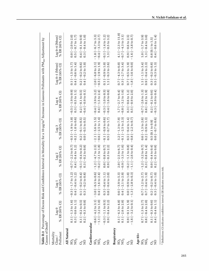
265


Tabl

e D

.3

Per

cen

tage

of

Exc

ess

Ris

k an

d C

onfi

den

ce I

nte

rval

in

Mor

tali

ty f

or a

10-

µg/

m3

Incr

ease

in

Gas

eou

s P

ollu

tan

ts w

ith

PM

10 A

dju

stm

ent

by

Cau

ses

of D

eath

a

Mor

tali

ty

Cla

ss /

P

ollu

tan

tL

ag 0

% E

R (

95%

CI)

Lag

1%

ER

(95

% C

I)L

ag 2

% E

R (

95%

CI)

Lag

3%

ER

(95

% C

I)L

ag 4

% E

R (

95%

CI)

Lag

0–1

(M

ean

)%

ER

(95

% C

I)L

ag 0

–4 (

Mea

n)

% E

R (

95%

CI)

All

Nat

ura

lS

O2

0.1

(�1.

3 to

1.6

)�

0.3

(�1.

7 to

1.2

)�

0.7

(�2.

2 to

0.7

)�

0.5

(�1.

9 to

1.0

)�

0.5

(�1.

9 to

0.9

)0.

1 (�

1.5

to 1

.7)

0.0

(�2.

0 to

2.0

)N

O2

0.3

(�0.

6 to

1.1

)0.

4 (�

0.4

to 1

.2)

0.4

(�0.

4 to

1.2

)�

0.2

(�1.

0 to

0.6

)0.

3 (�

0.5

to 1

.1)

0.4

(�0.

6 to

1.4

)0.

5 (�

0.7

to 1

.7)

O3

0.1

(�0.

2 to

0.5

)0.

1 (�

0.2

to 0

.4)

�0.

1 (�

0.4

to 0

.2)

0.2

(�0.

1 to

0.5

)0.

2 (�

0.1

to 0

.5)

0.2

(�0.

2 to

0.6

)0.

4 (�

0.1

to 0

.9)

NO

0.2

(�0.

3 to

0.8

)0.

3 (�

0.2

to 0

.8)

0.3

(�0.

2 to

0.8

)0.

0 (�

0.5

to 0

.5)

�0.

4 (�

0.9

to 0

.1)

0.4

(�0.

2 to

1.0

)0.

3 (�

0.4

to 1

.0)

Car

dio

vasc

ula

rS

O2

�0.

6 (�

4.2

to 3

.1)

�3.

0 (�

6.5

to 0

.6)

�1.

2 (�

4.7

to 2

.5)

�2.

1 (�

5.6

to 1

.5)

�0.

4 (�

3.9

to 3

.2)

�2.

0 (�

6.0

to 2

.1)

�1.

8 (�

6.7

to 3

.3)

NO

2�

1.1

(�3.

2 to

1.0

)0.

4 (�

1.6

to 2

.4)

�0.

2 (�

2.1

to 1

.8)

�0.

6 (�

2.5

to 1

.4)

0.4

(�1.

5 to

2.4

)�

0.5

(�2.

9 to

1.9

)�

0.4

(�3.

3 to

2.7

)

O3

�0.

3 (�

1.1

to 0

.5)

0.3

(�0.

4 to

1.1

)0.

0 (�

0.8

to 0

.7)

�0.

1 (�

0.9

to 0

.6)

�0.

3 (�

1.0

to 0

.5)

0.1

(�0.

9 to

1.0

)�

0.1

(�1.

4 to

1.2

)N

O0.

9 (�

0.4

to 2

.2)

0.8

(�0.

4 to

2.0

)0.

9 (�

0.3

to 2

.2)

0.5

(�0.

7 to

1.7

)�

0.4

(�1.

6 to

0.8

)1.

1 (�

0.3

to 2

.6)

1.3

(�0.

5 to

3.2

)

Res

pir

ator

yS

O2

0.1

(�4.

3 to

4.8

)0.

6 (�

3.9

to 5

.3)

2.0

(�2.

5 to

6.7

)3.

2 (�

1.3

to 7

.9)

1.7

(�2.

7 to

6.4

)0.

7 (�

4.3

to 6

.0)

4.1

(�2.

3 to

11.

0)N

O2

0.1

(�2.

6 to

2.8

)0.

4 (�

2.1

to 2

.9)

�0.

9 (�

3.3

to 1

.6)

�0.

1 (�

2.5

to 2

.3)

�0.

8 (�

3.2

to 1

.6)

0.3

(�2.

7 to

3.4

)�

0.7

(�4.

3 to

3.1

)

O3

0.9

(�0.

1 to

1.9

)0.

0 (�

0.9

to 1

.0)

�0.

2 (�

1.1

to 0

.8)

0.5

(�0.

4 to

1.4

)0.

3 (�

0.6

to 1

.2)

0.7

(�0.

5 to

1.9

)0.

9 (�

0.6

to 2

.5)

NO

�1.

6 (�

3.2

to 0

.1)

�1.

3 (�

2.8

to 0

.3)

�1.

1 (�

2.6

to 0

.4)

�0.

8 (�

2.2

to 0

.7)

0.5

(�0.

9 to

2.0

)�

1.8

(�3.

6 to

0.0

)�

1.6

(�3.

8 to

0.7

)

Age

65+

SO

20.

7 (�

1.3

to 2

.7)

0.7

(�1.

2 to

2.7

)�

1.2

(�3.

2 to

0.7

)0.

6 (�

1.3

to 2

.6)

�0.

7 (�

2.6

to 1

.3)

1.1

(�1.

1 to

3.4

)1.

0 (�

1.7

to 3

.9)

NO

20.

8 (�

0.4

to 2

.0)

0.7

(�0.

4 to

1.9

)0.

3 (�

0.8

to 1

.4)

0.2

(�0.

9 to

1.3

)0.

8 (�

0.2

to 1

.9)

0.9

(�0.

4 to

2.3

)1.

3 (�

0.4

to 3

.0)

O3

0.1

(�0.

3 to

0.6

)0.

2 (�

0.2

to 0

.7)

0.0

(�0.

4 to

0.4

)0.

5 (0

.1 t

o 0.

9)0.

2 (�

0.2

to 0

.6)

0.3

(�0.

2 to

0.8

)0.

8 (0

.1 t

o 1.

5)N

O0.

4 (�

0.4

to 1

.1)

0.3

(�0.

4 to

1.0

)0.

2 (�

0.5

to 0

.8)

0.0

(�0.

7 to

0.6

)�

0.3

(�0.

9 to

0.4

)0.

5 (�

0.3

to 1

.3)

0.4

(�0.

6 to

1.4

)

a D

efin

itio

ns:

CI

ind

icat

es c

onfi

den

ce i

nte

rval

; ER

in

dic

ates

exc

ess

risk

.

266


Tabl

e D

.4.

Per

cen

tage

of

Exc

ess

Ris

k in

Mor

tali

ty a

nd

Con

fid

ence

In

terv

al f

or a

10-

µg/

m3

Incr

ease

in

PM

10 w

ith

Gas

eou

s A

dju

stm

ent

by C

ause

s of

Dea

tha

Mor

tali

ty C

lass

/ A

dju

sted

P

ollu

tan

tL

ag 0

PM

10%

ER

(95

% C

I)L

ag 1

PM

10%

ER

(95

% C

I)L

ag 2

PM

10%

ER

(95

% C

I)L

ag 3

PM

10%

ER

(95

% C

I)L

ag 4

PM

10%

ER

(95

% C

I)

Lag

0–1

(M

ean

) P

M10

% E

R (

95%

CI)

Lag

0–4

(M

ean

) P

M10

% E

R (

95%

CI)

All

Nat

ura

lS

O2

1.2

(0.7

to

1.6)

1.0

(0.6

to

1.4)

1.0

(0.6

to

1.4)

0.9

(0.4

to

1.3)

0.3

(�0.

1 to

0.7

)1.

2 (0

.8 t

o 1.

7)1.

4 (0

.9 t

o 2.

0)N

O2

1.0

(0.3

to

1.7)

0.7

(0.0

to

1.4)

0.6

(0.0

to

1.3)

0.9

(0.3

to

1.6)

0.1

(�0.

6 to

0.7

)1.

0 (0

.2 t

o 1.

8)1.

1 (0

.1 t

o 2.

0)

O3

1.1

(0.6

to

1.5)

0.9

(0.4

to

1.3)

1.0

(0.5

to

1.4)

0.6

(0.2

to

1.1)

0.1

(�0.

4 to

0.6

)1.

1 (0

.6 t

o 1.

7)1.

1 (0

.5 t

o 1.

8)N

O1.

0 (0

.6 t

o 1.

5)0.

8 (0

.4 t

o 1.

3)0.

8 (0

.3 t

o 1.

2)0.

8 (0

.4 t

o 1.

2)0.

4 (0

.0 t

o 0.

9)1.

1 (0

.6 t

o 1.

6)1.

3 (0

.7 t

o 1.

9)

Car

dio

vasc

ula

rS

O2

1.6

(0.5

to

2.7)

2.0

(0.9

to

3.1)

1.7

(0.6

to

2.8)

1.1

(0.0

to

2.1)

�0.

1 (�

1.1

to 1

.0)

2.1

(0.9

to

3.3)

2.0

(0.6

to

3.4)

NO

22.

3 (0

.5 t

o 4.

2)1.

4 (�

0.3

to 3

.1)

1.7

(0.0

to

3.4)

1.3

(�0.

4 to

3.0

)�

0.4

(�2.

1 to

1.3

)2.

3 (0

.2 t

o 4.

3)2.

1 (�

0.4

to 4

.7)

O3

1.8

(0.6

to

3.0)

1.4

(0.2

to

2.6)

1.6

(0.4

to

2.8)

0.9

(�0.

3 to

2.1

)0.

1 (�

1.0

to 1

.3)

1.8

(0.5

to

3.2)

2.0

(0.3

to

3.6)

NO

1.1

(�0.

1 to

2.3

)1.

3 (0

.2 t

o 2.

4)1.

2 (0

.1 t

o 2.

3)0.

6 (�

0.5

to 1

.7)

0.1

(�1.

0 to

1.2

)1.

4 (0

.1 t

o 2.

71.

3 (�

0.2

to 2

.9)

Res

pir

ator

yS

O2

1.0

(�0.

4 to

2.4

)0.

7 (�

0.6

to 2

.0)

0.9

(�0.

4 to

2.2

)1.

0 (�

0.3

to 2

.3)

0.5

(�0.

8 to

1.8

)0.

9 (�

0.5

to 2

.4)

1.4

(�0.

3 to

3.1

)N

O2

0.9

(�1.

3 to

3.2

)0.

5 (�

1.6

to 2

.7)

1.7

(�0.

4 to

3.9

)1.

4 (�

0.7

to 3

.5)

1.2

(�0.

8 to

3.3

)0.

8 (�

1.7

to 3

.3)

2.2

(�0.

9 to

5.4

)

O3

0.3

(�1.

2 to

1.8

)0.

7 (�

0.7

to 2

.2)

1.2

(�0.

2 to

2.7

)0.

9 (�

0.5

to 2

.4)

0.4

(�1.

0 to

1.9

)0.

5 (�

1.2

to 2

.2)

1.0

(�1.

0 to

3.1

)N

O1.

8 (0

.2 t

o 3.

3)1.

3 (�

0.1

to 2

.8)

1.6

(0.2

to

3.0)

1.6

(0.3

to

3.0)

0.4

(�0.

9 to

1.8

)1.

9 (0

.2 t

o 3.

5)2.

4 (0

.5 t

o 4.

3)

Age

65+

SO

21.

4 (0

.8 t

o 2.

0)1.

0 (0

.5 t

o 1.

6)1.

2 (0

.7 t

o 1.

8)1.

1 (0

.5 t

o 1.

7)0.

8 (0

.2 t

o 1.

4)1.

4 (0

.8 t

o 2.

1)1.

8 (1

.1 t

o 2.

6)N

O2

0.9

(0.0

to

1.9)

0.6

(�0.

3 to

1.6

)0.

9 (0

.0 t

o 1.

8)1.

0 (0

.1 t

o 1.

9)0.

1 (�

0.8

to 1

.1)

0.9

(�0.

2 to

2.0

)1.

0 (�

0.3

to 2

.4)

O3

1.4

(0.7

to

2.0)

0.9

(0.3

to

1.6)

1.1

(0.5

to

1.7v

0.7

(0.1

to

1.3)

0.5

(�0.

1 to

1.2

)1.

3 (0

.6 t

o 2.

0)1.

3 (0

.5 t

o 2.

2)N

O1.

3 (0

.6 t

o 1.

9)1.

0 (0

.4 t

o 1.

6)1.

0 (0

.4 t

o 1.

7)1.

2 (0

.6 t

o 1.

8)0.

8 (0

.2 t

o 1.

4)1.

3 (0

.6 t

o 2.

0)1.

8 (0

.9 t

o 2.

6)

a D

efin

itio

ns:

CI

ind

icat

es c

onfi

den

ce i

nte

rval

; ER

in

dic

ates

exc

ess

risk

.


APPENDIX E. HEI Quality Assurance Statement

The conduct of this study was subjected to periodic,independent audits by a team from Hoover Consultants.This team consisted of auditors with experience in toxicol-ogy, epidemiology, and air quality data. The auditsincluded in-process monitoring of study activities for con-formance to the study protocol and examination of recordsand supporting data. The dates of each audit are listed inthe table below with the phase of the study examined.

QUALITY ASSURANCE AUDITS

Date Phase of Study

May 26–27, 2005 Data for mortality, air quality parame-ters, and meteorology were audited.Documentation was examined for per-sonnel qualifications and experience.During this site visit, data were au-dited in the 5- and 10-Month Progressreports supplied by HEI. This studywas conducted in accordance with anindividual study protocol that coveredthe unique features of the Bangkokstudy and a combined protocol for thecoordinated time-series analysis. Studydocumentation was reviewed to deter-mine that it met the requirements ofboth protocols. Statements in the textof the reports were compared to thesubsequent tables, figures, and datafiles. Reports were reviewed for inter-nal consistency. Air pollution datawere provided by the investigators aselectronic copies of the original zippedtext files of 1997–2003 hourly data de-livered by the Pollution Control De-partment. The investigators provided aspreadsheet of daily data used to pro-duce daily citywide averages for the ep-idemiologic analysis and the summarystatistics in the 10-Month Progress Re-port. Dr. Patcharawadee Suwanathadaof the Pollution Control Departmentwas present to answer questions andprovide background. The audit teammade a series of database queries de-signed to validate all of the numbers pre-sented in the 10-Month Progress Re-port (with the exception of Table 3.1,death counts by district, for the years

1997 and 1998 since these years wereto be dropped from the study). In addi-tion, the auditors visited District 10(Mean-Buri) to compare a sample of50 death certificates to 12 different vari-ables per certificate in the study data-base. The underlying cause of deathwas verbally translated by study per-sonnel and compared to the ICD-10code that had been assigned. The auditteam then compared these assignedcodes to the written descriptions of theunderlying cause of death in the ICD-10 Classification System.

April 7, 2008 A draft of the final study report wasexamined for internal consistencyand conformance with the study pro-posal. Comments were provided toHEI via e-mail.

A written report of the first inspection was provided tothe Director of Science of the Health Effects Institute whotransmitted these findings to the Principal Investigator.These quality assurance audits demonstrated that thestudy was conducted by experienced professionals inaccordance with the study protocols. The report appears tobe an accurate representation of the study.

B. Kristin HooverHoover Consultants

ABOUT THE AUTHORS

Nuntavarn Vichit-Vadakan, Dr. PH., has been involved inair pollution research in Thailand for many years. Herwork in environmental epidemiology in Thailand has ledto policy changes and the development of mitigation mea-sures (environmental management interventions). She wasthe lead author on three labor- and data-intensive panelstudies examining the effects of PM10 and PM2.5 in Thai-land and has led many training sessions for Thai studentsand faculty in epidemiologic methods.

Nitaya Vajanapoom has a Ph.D. in epidemiology from theUniversity of North Carolina and is an environmental epi-demiologist at Thammasat University in Bangkok. She haspublished studies on air pollution and mortality in Thai-land (Vajanapoom et al. 2002) and is one of the lead epide-miologists on a five-year study that examines the health

267


effects of air pollution from a lignite power plant locatedin Lampang province, Thailand. Her work has contributedto the Thai government’s efforts in setting PM2.5 standards.

Bart Ostro, Ph.D., has published more than 70 studies link-ing air pollution to adverse health, including studies inThailand (Ostro et al. 1999), in other developing countriesincluding Chile, and in developed countries outside theUnited States. He has also worked with researchers in China,India, Indonesia, Malaysia, Mexico, Nepal, and Sri Lankain collecting or evaluating data, developing epidemiologicstudies, or assessing health effects. Finally, he has led sev-eral training programs for Thai students and faculty.

OTHER PUBLICATIONS RESULTINGFROM THIS RESEARCH

Vichit-Vadakan N, Vajanapoom N, Ostro B. 2008. The Pub-lic Health and Air Pollution in Asia (PAPA) project: Estimat-ing the mortality effects of particulate matter in Bangkok,Thailand. Environ Health Perspect 116:1179–1182.

Wong CM, Vichit-Vadakan N, Kan H, Qian Z, the PAPAProject Team. 2008. Public Health and Air Pollution inAsia (PAPA): A multicity study of short-term effects ofair pollution on mortality. Environ Health Perspect 116:1195–1202.

268

ABBREVIATIONS AND OTHER TERMS

AR1 model with first-order autocorrelation term

CI confidence interval

COPD chronic obstructive pulmonary disease

df degrees of freedom

dow day of week

ER excess risk

ICD-10 International Classification of Diseases, 10th revision

IQR interquartile range

LRI lower respiratory infection

NO nitric oxide

NO2 nitrogen dioxide

O3 ozone

OEP Office of Environmental Policy and Planning

PACF partial autocorrelation function

PAPA Public Health and Air Pollution in Asia

PM particulate matter

PM2.5 particulate matter � 2.5 µm in aerodynamic diameter

PM10 particulate matter � 10 µm in aerodynamic diameter

RH relative humidity

RR relative risk

SO2 sulfur dioxide

U.S. EPA U.S. Environmental Protection Agency

WHO World Health Organization

COMMENTARYHealth Review Committee

Research Report 154, Part 3. Estimating the Effects of Air Pollution on Mortality in Bangkok, Thailand, N. Vichit-Vadakan et al.

BACKGROUND

The study by Dr. Vitchit-Vadakan of Thammasat Univer-sity, Pathumthani, Thailand, and colleagues, titled Esti-mating the Effects of Air Pollution on Mortality in Bangkok,Thailand, was conducted as part of a coordinated suite oftime-series studies of the health effects of short-term expo-sure to air pollution in major Asian cities, a major compo-nent of HEI’s Public Health and Air Pollution in Asia(PAPA*) program. Information on the origins, objectives,and scope of the health and environmental conditions inBangkok, Thailand, and a brief review of previous epide-miologic research on the health effects of air pollution inBangkok are presented in the Overview for the four PAPAtime-series studies in this volume.

Previous time-series studies of daily pollutant levelsand mortality conducted predominantly in North Americaand Europe have found that increasing levels of air pollu-tion were associated with increasing mortality from varyingcauses (Kinney and Ozkaynak 1991; Anderson et al. 1996;Sunyer et al. 1996; Wietlisbach et al. 1996; Touloumi et al.1997; Saez et al. 1999). Thailand is one of several Asiancountries that has adopted national ambient air quality stan-dards for pollutants, including nitrogen dioxide (NO2),sulfur dioxide (SO2), ozone (O3), and particulate matter(PM) with an aerodynamic diameter � 10 µm (PM10).Monitoring studies conducted in Bangkok have shownthat ambient levels of PM10 frequently exceed that of theThai government’s national daily standards of 120 µg/m3

(Jinsart et al. 2002).

SPECIFIC AIMS

In response to a request by the HEI Research Committee,Dr. Vitchit-Vadakan submitted an application to investigatethe impact of air pollution on daily mortality in Bangkokusing six years of data (1996–2001). That time periodincluded an economic recession (June 1996–December1997). Hence, the study also sought to evaluate the impactof economic recession on traffic-related air pollution andany possible effects on mortality rates. The Committee con-sidered these aims responsive to the objective of the PAPAprogram and recommended the study for funding. The Com-mittee also recommended funding time-series studies inthree other Asian cities: Hong Kong, Shanghai, and Wuhan.

The originally proposed specific aims of the presentstudy were as follows:

1. Using PM10 monitoring data, quantify the associa-tion between ambient air pollution and mortality inBangkok.

2. Using stratified analyses, examine the potential effectmodification by sex and age in the association be-tween air pollution and mortality.

3. Examine disease-specific associations between mortal-ity and air pollution.

4. Examine whether reductions in local traffic levels dur-ing an economic recession affected mortality rates andthe resultant concentration–response functions.

After the study had been completed and the report sub-mitted, the HEI Review Committee was not convinced thatthe economic analyses were informative and suggested thatthe revised final report exclude this aim. Thus, the finalreport accepted by HEI had the following specific aims:

1. To evaluate the association between levels of ambientparticulate and gaseous air pollutants (PM10, O3, NO2,and SO2) and daily mortality due to all natural causes(nonaccidental) in Bangkok.

2. To evaluate both disease-specific and age-specificmortality in the identification of subgroups at partic-ular risk for the adverse health effects of air pollution.

3. To conduct extensive sensitivity analyses of the resultsin order to examine the influence of model specification,smoothing methods, lag structure, and copollutants.

Dr. Nuntavarn Vichit-Vadakan’s 2-year study “Estimating the MortalityEffects of Air Pollution in Bangkok, Thailand” began in June 2004. Totalexpenditures were $119,055. The draft Investigators’ Report from Vichit-Vadakan and colleagues was received for review in September 2006. Therevised report received in October 2007 was accepted for publication inDecember 2007. During the review process, the HEI Health Review Commit-tee and the investigators had the opportunity to exchange comments and toclarify issues in both the Investigators’ Report and the Review Committee’sCommentary.

This document has not been reviewed by public or private party institu-tions, including those that support the Health Effects Institute; therefore, itmay not reflect the views of these parties, and no endorsements by themshould be inferred.

*A list of abbreviations and other terms appears at the end of the Investiga-tors’ Report.

Health Effects Institute Research Report 154 © 2010 269

Commentary on Investigators’ Report by Vichit-Vadakan et al.

DATA SOURCES

The investigators used three sets of data — mortality, airpollution, and meteorologic — which were compiled elec-tronically by the responsible government agency.

Mortality data were obtained from the Bureau of Regis-tration Administration for the Bangkok Metropolitan Regionfor the period June 1, 1997, to May 31, 2003. Data consis-tency checks comparing the electronic mortality data todeath certificates revealed that a significantly lower numberof deaths were recorded for the period June 1, 1997, to De-cember 31, 1998. Thus this period was excluded from theanalyses, and the study period was changed to January 1,1999, to December 31, 2003. Causes of death were classi-fied using the tenth revision of the International Classifica-tion of Diseases (ICD-10).

Air pollution data were collected from several sets ofmonitors, set up by the Pollution Control Department ofthe Thai Ministry of Natural Resources and Environment tomeasure air pollution in Bangkok. Hourly measurementsof PM10 levels were available for 5 ambient and 7 roadsidemonitoring stations; 10 stations measured hourly ambientNO2, SO2, and nitric oxide (NO), while 8 stations mea-sured hourly ambient O3. Since there was substantial roadtraffic around the 7 roadside monitors, the researchers usedonly the PM10 data from the 5 ambient monitors, believingthat these measurements best represented actual popula-tion exposures in Bangkok. As with all of the PAPAstudies, carbon monoxide was not included in the anal-yses. Individual monitors were included in the study ifdata from the monitor were determined to be internallyconsistent, were not heavily influenced by a local air pol-lution source, and met the inclusion criteria for individualpollutants described in the Common Protocol (found at theend of this volume) and Integrated Discussion (found inPart 5 of this volume).

Daily meteorologic data were obtained from the Bang-kok metropolitan weather station for the study period. Thedata included average daily temperature and average dailyrelative humidity (RH).

DATA ANALYSIS

To assess the short-term effect of PM10 and gaseous pol-lutants on daily mortality, the investigators used the statis-tical analyses that were developed by all participants inthe PAPA project as part of the Common Protocol (see theIntegrated Discussion in Part 5 of this volume).

The investigators determined the best core model forall natural mortality in accordance with the agreed-upon

Common Protocol: a model using 6 degrees of freedom (df)minimized the partial autocorrelation, and so the investi-gators used this specification in all subsequent analyses.The core model used a two-day average of lag 0 and lag 1(lag 0–1 day), but the investigators also examined lags ofup to 5 days and moving averages of up to 5 days. A day-of-the-week term was also included. This core model for alldeaths due to natural causes was used for each of the sub-categories of cause of death, specifically, cardiopulmonary(cardiovascular and respiratory), cardiovascular separately(including subcategories of ischemic heart disease, stroke,and conduction disorders), respiratory separately (includ-ing subcategories of chronic obstructive pulmonary dis-order [COPD] and asthma), “senility,” non-cardiopulmonary(natural), and accidental.

They also performed several sensitivity analyses inorder to test their modeling assumptions, including the fit-ting of models with different lags for PM10; different setsof degrees of freedom for time and weather; different lagsof temperature and RH; and penalized splines in place ofnatural splines for time and weather. They also fitted co-pollutant models that assessed the effects of PM10, adjustedfor gaseous pollutants. In addition, they performed a sensi-tivity analysis that considered an influenza epidemic as apotential confounder of pollutant effects, defining “influ-enza epidemic” as a weekly respiratory mortality countgreater than the 90th percentile of the mean frequency(count) of respiratory mortality for each year.

RESULTS

Commentary Tables 1–3 and the following paragraphssummarize the key findings. All analysis results are pre-sented as excess risk (ER) per 10 µg/m3 of pollutant, calcu-lated from relative risk (RR) as ER = (RR � 1) � 100.

DAILY MORTALITY AND POLLUTANT INFORMATION

Commentary Table 1, which summarizes informationfrom Table 2 of the Vichit-Vadakan Investigators’ Report,shows that during the study period (1999–2003) Bangkokhad an average of 95 deaths per day from all naturalcauses. An average of 13 deaths per day were attributed tocardiovascular causes, 8 deaths per day were due to respi-ratory causes, and 14 deaths were attributed to “senility.”Dr. Vitchit-Vadakan included “senility” as an endpointbecause there were lower-than-expected daily counts ofdeaths in the elderly that were attributed to cardiovasculardiseases and a correspondingly high number attributed to“senility.” Bangkok recorded an average of 45 deaths per

270

Health Review Committee

Commentary Table 1.

Average Daily Mortality in Bangkok During Study Period for Total Nonaccidental Mortality and Selected Other Categories of Cause of Death

a

Cause of Death Deaths per Day (SD)

All natural (nonaccidental) 95 (12.1)Cardiovascular 14 (4.3)Respiratory 8 (3.1)

“Senility”

14 (4.2)

a

Definition: SD indicates standard deviation.

Commentary Table 2.

Mean 24-Hour Pollutant Concentrations, Temperature, and Relative Humidity in Bangkok During Study Period

a

Pollutant /MeteorologicMeasurement Mean (SD) Maximum

PM

10

(µg/m

3

) 52.1 (20.1) 169.2SO

2

(µg/m

3

) 13.2 (4.8) 61.2NO

2

(µg/m

3

) 44.7 (17.3) 139.6O

3

(µg/m

3

) 59.4 (26.4) 180.6NO (µg/m

3

) 28.0 (14.2) 126.9

Temperature (

�

C) 28.9 (1.7) 33.6

RH (%)

72.8 (8.3)

95.0

a

Definitions: RH indicates relative humidity; SD indicates standard deviation.

day in persons age 65 or older (see Vichit-Vadakan Investi-gators’ Report Table 1).

Commentary Table 2 shows the mean 24-hour concen-trations of PM10, SO2, NO2, O3, and NO and mean temper-ature and RH during the study period.

The investigators reported relatively high correlationsbetween daily levels of PM10 and NO2 (r = 0.71), PM10 andO3 (r = 0.55), and O3 and NO2 (r = 0.62) (Vichit-VadakanInvestigators’ Report Table 5). Mean temperature andhumidity were provided for the entire year as the rela-tively low standard deviation demonstrated the relativelyminimal seasonal variation in Bangkok’s weather due to itstropical location and local weather conditions (see Vichit-Vadakan Investigators’ Report Table 6).

ASSOCIATIONS BETWEEN DAILY MORTALITY AND INDIVIDUAL POLLUTANTS

Commentary Table 3 summarizes the main findings ofassociations between individual pollutants and daily deathsby cause of mortality in single-pollutant models (shown inTable 7a of the Vichit-Vadakan Investigators’ Report).

Commentary Table 3. Excess Risk of Mortality per 10-µg/m3

Cause of Death(All Ages Unless Specified)

PM10% ER (95% CI)

SO2% ER (95% CI)

All natural 1.3 (0.8 to 1.7) 1.6 (0.1 to 3.2)Cardiovascular 1.9 (0.8 to 3.0) 0.8 (�3.0 to 4.7)Respiratory 1.0 (�0.4 to 2.4) 1.7 (�3.1 to 6.6)Non-cardiopulmonary

(nonaccidental) 1.2 (0.8 to 2.0) 1.8 (0.1 to 3.5)Accidental 0.1 (�2.3 to 2.6) 0.0 (�8.0 to 8.8)Age 65+ yr 1.5 (0.9 to 2.1) 2.8 (0.7 to 5.0)

a Definitions: CI indicates confidence interval; ER indicates excess risk.

Findings from the main analysis indicate that short-termincreases in the concentrations of all of the air pollutants(PM10, NO2, SO2, O3, and NO), using the mean pollutantconcentrations at lag 0–1 day, were associated with in-creased daily nonaccidental all-cause mortality. Associa-tions between increases in the pollutant concentrationsand respiratory mortality were positive (except for NO) butquite imprecise, and a few statistically significant associa-tions were observed for some pollutants in mortality sub-groups. While no pollutant was associated with increases inaccidental mortality, all of the pollutants were significantlyassociated with increases in natural, non-cardiopulmonarymortality. Effect estimates (excess risk) were largest inpeople 65 or older and, except for SO2, in those who diedof cardiovascular causes and in those whose cause of deathwas termed “senility” (Vichit-Vadakan Investigators’ ReportTable 7a).

271

Increase in Pollutants at Lag 0–1 Daya

NO2% ER (95% CI)

O3% ER (95% CI)

NO% ER (95% CI)

1.4 (0.9 to 1.9) 0.6 (0.3 to 0.9) 1.1 (0.6 to 1.6) 1.8 (0.5 to 3.1) 0.8 (0.0 to 1.6) 2.0 (0.7 to 3.2) 1.0 (�0.6 to 2.7) 0.9 (�0.1 to 1.9) �0.7 (�2.3 to 0.9)

1.4 (0.8 to 2.0) 0.6 (0.2 to 0.9) 1.1 (0.5 to 1.7)�0.1 (�3.0 to 2.8) 0.0 (�1.8 to 1.8) 0.8 (�2.0 to 3.6) 1.8 (1.1 to 2.6) 0.8 (0.4 to 1.3) 1.3 (0.6 to 2.0)


Results from sensitivity analyses demonstrated thatpositive associations between individual pollutants anddaily mortality in single-pollutant models were largelyrobust to differences in model specifications for the degreeof smoothing for time, choice of regression spline (naturalor penalized), and adjustment for confounders including“influenza.” There was greater sensitivity, however, toinclusion of alternative lags for humidity and tempera-ture on the effect on total (all natural) mortality (Vichit-Vadakan Investigators’ Report Table 11), especially for NO2and NO. The effect of PM10 was also substantially reducedwith longer-term weather lags but was still greater thanzero, while those of SO2 and O3 were largely unaffected. Intwo-pollutant models (Vichit-Vadakan Investigators’ ReportTable 13), the association of PM10 with daily total (all nat-ural) and cardiovascular mortality was relatively robust toadjustment for gaseous copollutants. However, the associ-ations between the gaseous pollutants and daily mortalitywere generally sensitive to PM10 adjustment (Vichit-Vadakan Investigators’ Report Table 12).

HEI EVALUATION OF THE STUDY

ASSESSMENT OF HEALTH OUTCOMES

The mortality health endpoints commonly used in time-series studies were also used in the Bangkok study. Hence,total mortality (after excluding “accidental” deaths) andthe large strata of cardiovascular and respiratory deathswere included as endpoints. In addition, partly because ofthe large number of daily deaths in Bangkok, effects in alarge number of additional cause-of-death strata wereexamined, specifically, ischemic heart disease, lower res-piratory infection, COPD, and asthma. While the classifi-cation of cause of death into cardiopulmonary and non-cardiopulmonary categories should be relatively valid,finer cause-of-death strata would be expected to be less so,complicating the discernment of ischemic heart diseasefrom other causes of cardiovascular deaths.

The findings in this Bangkok study showing that theeffect estimates were generally larger in the elderly (age 65or older) and in those who died of cardiovascular causeswere similar to those in most air pollution time-seriesstudies. However, complicating the disease-specific find-ings in Bangkok, especially those involving cardiovascularcauses of death, is the use of “senility” as a cause of death.The authors of the report speculate that the “senility”coding may be essentially capturing a category of cardio-vascular deaths; their point is supported by the unusuallylow percentage of deaths due to cardiovascular diseasecaptured by the coding of only “cardiovascular.” Also, the

pattern and size of the pollution effect estimates in thesenility cause-of-death stratum mirror those in the cardio-vascular stratum, further supporting the authors’ specula-tion about the misclassification of cardiovascular deaths inthe oldest age categories.

POLLUTANT CONCENTRATION MONITORING AND EXPOSURE ESTIMATION IN BANGKOK

Similar to the other PAPA studies, the Bangkok study re-lied on using routine monitoring data from the government-operated network, which is based on the U.S. Environ-mental Protection Agency (EPA) standard methods. Themonitors are assessed, and the data are routinely checkedby the local agency, though no additional evaluation (e.g.,using collocated sampling for a limited period) was donefor this study. Only four days were found to not have suffi-cient observations to calculate a daily average, and thatwas only for PM10. For the main results, the investigatorsdid not “center” concentrations when calculating dailymeans, which would have limited noise caused by varia-tion in the pattern of missing values. The Committee con-sidered this a limitation, though when centered valueswere used in the sensitivity analyses in this study (Vichit-Vadakan Investigators’ Report Table 9), only the results forSO2 changed appreciably. Similar to studies in many othercities, the Bangkok study found that observations of O3and PM10 at different monitor sites (Vichit-Vadakan Inves-tigators’ Report Table B.3 in Appendix B) tended to behighly correlated (Spearman correlations typically above0.5, often around 0.8), while NO2 was somewhat less so.SO2 and NO tended to have low, and sometimes nega-tive, correlations across monitors. This would suggest thatassessment of area-wide exposures to SO2 and NO, evenusing averages, was more likely to contain meaningfulexposure measurement error. On the other hand, ambientexposures to O3 and PM10 are likely to be well representedby the calculated averages because site-to-site correlationswere high.

No additional calculations were done to help assess thepotential exposure error for any of the pollutants or to seeif the correlations between stations were dependent ondistance or were influenced by sources of pollution andother land-use features near the monitors. The average cal-culated is used to represent exposure across the entirestudy area, and there is no consideration of the extent of orlack of agreement between the calculated averages and theobservations at each monitor, as the investigators do notshow how the averages used correlate with individual sta-tion data. Showing the statistical comparisons betweenarea averages and individual monitor observations couldhave shed light on which stations are most representative

272


of the region and if one monitor had excessive influence onthe results.

Correlations between the pollutant concentrations(Vichit-Vadakan Investigators’ Report Table B.1) show thatNO2 and PM10 have the highest correlation (0.71), sug-gesting a common source (e.g., automotive emissions). O3–NO2 and O3–PM10 concentrations are moderately corre-lated (0.62 and 0.55, respectively), suggesting the photo-chemical formation of a fraction of the PM2.5 and thepotential for limited confounding. NO and SO2 are nothighly correlated with any of the other pollutants, sug-gesting unique sources, local sources or conditions, and/ordifferent atmospheric dynamics.

Unlike in most time series, NO was included as a pol-lutant of interest in Bangkok. In general, it is not knownhow the estimates of the health effects associated with NOare best interpreted. NO concentrations, much like carbonmonoxide, are spatially very heterogeneous in urban areasdue in large part to the much higher concentrations inproximity to roadways and to the fact that NO is rapidlyconverted to NO2 in the presence of O3. One would expectthat averaging the daily concentrations of NO and NO2would result in considerable exposure measurement error,certainly to a greater extent than with the more spatiallyhomogeneous pollutants such as PM and O3.

Also similar to the other PAPA studies, this study hadonly a very brief characterization of the regional sourcesand dynamics of the pollutants. Further, there was no dis-cussion of how specific sources may have impacted spe-cific monitoring.

STATISTICAL METHODS

Aspects of the statistical methods that were common toall four PAPA studies in this phase are discussed in theIntegrated Discussion (in Part 5 of this volume). Here wecomment on the specifics of the statistical analysis in theBangkok study.

The results of the sensitivity analyses of key results tothe degrees of freedom (up to 15 df/year) in the time smooth-ers (see Vichit-Vadakan Investigators’ Report Table 10) werereassuring, with little sensitivity identified. There wasgreater sensitivity to the inclusion of alternative lags (lags1, 2, 3, 1–2 mean, or 3–7 mean) for humidity and tempera-ture (Vichit-Vadakan Investigators’ Report Table 11). Forexample, the excess risk from NO2 was reduced from 1.4%(95% confidence interval [CI], 0.9–1.9) in the core modelto 0.3% (95% CI, �0.3–0.8) with lag 3–7 day mean weatherterms. The PM10 effect was more robust, but was also sub-stantially reduced, from 1.3% (95% CI, 0.8–1.7) to 0.8%(95% CI, 0.3–1.3) with the inclusion of the longer weatherlags. The effects of SO2 and O3 were largely unchanged.

This sensitivity to weather terms in the model wassomewhat surprising, given the absence of much tempera-ture variation in this tropical city. It may be that otheraspects of weather patterns influence both mortality andpollution in the rainy season. A limitation of these sensi-tivity analyses was that the investigators replaced the lag 0weather term with longer-lag terms, rather than adding thelonger-lag terms to the model with the lag 0 term. We notethat several investigators have found that distributed lagmodels (i.e., those that include several lags simultane-ously) are needed to capture weather effects well (Bragaet al. 2000; McMichael et al. 2008). Thus the Committee isconcerned that even if a 0-day lag for temperature fits bestout of the single-lag models considered, this does notexclude the possibility that other lags could additionallyconfound the pollution effects. The investigators also sug-gest that the longer lags for weather variables may beproxies for longer lags for pollution levels. This is plau-sible, but no more so than the possibility that there arelonger-lag weather effects that confound the short-lag pol-lution effects. A way to address this would be to fit distrib-uted lag models for both pollution and weather, which wasnot attempted in this report.

We agree that the Bangkok study team’s other investiga-tions of sensitivity showed broad robustness to theirmodel choices. These included replacing the natural by apenalized spline, adding a first-order autocorrelation term(though there is no detail given on the method used forthis), adjusting for influenza, and using a “centering”method to combine monitoring station daily concentra-tions. These sensitivity analyses provide confidence in thereported associations.

EPIDEMIOLOGIC ASPECTS

Features of Bangkok

As described by Vichit-Vakakan and coworkers, Bang-kok is a relatively large city and therefore experiences alarge number of deaths per day — on average, 95. Thisstudy, which included 5 years of data, has good statisticalpower consistent with all of the Asian cities in PAPA todetect statistically significant associations. This allows arealistic examination of stratified associations, such as thosestratified by cause of death (including “control” causes ofdeath) and age category. Relative to most cities in the West,the age distribution of the Bangkok population is young, andconsequently so is the age distribution of deaths. However,a younger age distribution may reduce the size of the popu-lation at risk of dying from exposure to air pollution, espe-cially if death is caused by cardiovascular disease, therebyeffectively reducing the power to detect effects relative to

273


similarly sized Western cities. This may be particularlyrelevant when focusing on specific categories of cause ofdeath where the daily counts are much smaller relative tomortality counts due to all natural causes.

Concentrations of air pollutants in Bangkok were highrelative to those typically measured in Western cities,although not as high as in two of the three cities in China(Wuhan and Shanghai) also included in this first wave ofPAPA studies. According to the investigators’ report, theprincipal source of PM in Bangkok is vehicular emissions.The chemical composition of PM is largely determined bysource contributions. To the extent that PM compositiondetermines the type and severity of health effects attrib-uted to PM exposure, PM effect estimates in Bangkoklikely reflect the composition of motor-vehicle–relatedPM. Issues regarding the interpretation and relevance ofhealth effects estimates from high-concentration settingsare discussed in the Integrated Discussion, which coversall five PAPA reports and is found in Part 5.

Weather in Bangkok is characterized by temperaturesand humidity that is high relative to that in Western cities,and the temperature and humidity in Bangkok are amongthe most extreme of the PAPA cities studied in this report.While high temperature is itself a risk factor for higherdaily mortality (McMichael et al. 2008), there is also someevidence that temperature modifies the effect of air pollu-tion on daily mortality, with higher temperatures enhancingthe pollution mortality effect (Hu et al. 2008; Stafoggia et al.2008). The findings from Wuhan in this set of PAPA stud-ies provide some further support for such an interaction.

Pollutant-specific Effects and Robustness

The primary pollutant-related findings in the Bangkoktime-series study were that associations with mortalityfrom various causes were observed for all of the air pol-lutants analyzed (PM10, NO2, SO2, NO, and O3 in single-pollutant models [not adjusted for other pollutants]). Forall of these pollutants, the estimates of relative risk per unitof pollutant concentration were higher than the averages inother cities in the United States (Dominici et al. 2005) andEurope (Katsouyanni 2003; HEI International ScientificOversight Committee 2004) and in the Asian cities in theother PAPA studies (see Part 5. Combined Analysis in thisvolume). This was most pronounced for PM10, for whichthe ER was 1.3% (95% CI, 0.8–1.7) in this analysis.

The effects of PM10 were largely insensitive to control-ling for the gaseous pollutants in two-pollutant models. Incontrast, the effects of NO2 and SO2 were largely sensitiveto the adjustment for PM10. However, even the effects ofPM10, as noted earlier in the discussion of the statisticalmethods, were sensitive to control for long temperature

lags. These findings indicate that the mortality effects ofshort-term pollutants in Bangkok are dominated by effectsfrom PM10.

As discussed more fully in the accompanying IntegratedDiscussion (in Part 5 of this volume), the intent of multipleregression modeling is to allow the estimated effects of anysingle variable (e.g., the concentration of one pollutant) tobe interpreted as the effect of that variable, controlled forthe effects of the other variables (e.g., concentrations ofother pollutants) included in the model. There are, how-ever, obstacles to this interpretation of multiple regres-sion effect estimates, including problems of model speci-fication, collinearity resulting from strong correlationsbetween concentrations of different air pollutants, differ-ential impacts of exposure measurement error, and resi-dual confounding across the different pollutants. There-fore, the extent to which multipollutant models, eventwo-pollutant models as used here, serve their intendedpurpose of allowing pollutant effect estimates to be inter-preted independent of the effects of other pollutants islimited. If PM10 concentrations provide better exposuremeasures in the time-series study design than concentra-tions of the other pollutants (as they do in this study whencompared with NO2 and SO2), the robustness of the PM10effect to the inclusion of other pollutants may indicate lesserror in the exposure measurements rather than a domi-nant effect of PM10.

Health Endpoints

Unlike in most time-series air pollution studies, therewas no strong evidence for associations between exposureto the pollutants and overall respiratory mortality in theBangkok study. It is not clear why there were no associa-tions for overall respiratory mortality, but there are somepossible explanations. Most respiratory mortality in West-ern countries is due to COPD (Kung et al. 2008). Sincecoded COPD deaths in Bangkok make up a much smallerproportion of respiratory deaths (only 25%) than in theother three cities, an association with overall respiratorymortality might not be seen if air pollution affected mainlythis specific disease. The same situation would result ifCOPD deaths were miscoded as another category, such as“senility.” The relatively small proportion of deaths codedas due to respiratory causes may also have led to impreci-sion in the resulting effect estimate. Substantial effectswere seen for the subcategories of death due to asthma andfor respiratory mortality in children less than 1 year old inthis study, especially those associated with PM10. It is alsostriking to note that the percentage of average daily deathsdue to cardiovascular or respiratory causes in Bangkok isconsiderably lower than it is in the three Chinese cities

274


studied in the PAPA program, and the number of deaths at-tributed to these causes in the older ages is proportionatelylower. Because of the very small number of daily deaths inthese subcategories, one must be especially cautious inplacing too much weight on these specific findings.

Analyzing the causes of death not anticipated to be dueto short-term exposure to air pollution might be useful forassessing the adequacy of this study’s methods, such as itspollutant exposure estimation or statistical modeling. Spe-cifically, if pollutant effects are found in these cause-of-death strata, one might be more skeptical of the findingsfor causes of death for which such effects were antici-pated. In this study, both “accidental” deaths and totalnon-cardiopulmonary deaths after excluding accidentaldeaths were used as “control” causes of death. No pol-lutant was associated with accidental causes of death, butincreases in all of the pollutants were associated withincreased non-cardiopulmonary deaths.

How are we to interpret the findings in the Bangkokstudy of associations for non-cardiopulmonary mortalitywith increases in all the pollutants? In general, such find-ings should prompt consideration of features of the studymethods. First, are the data derived from the pollutantmonitoring network adequate for the purpose of exposureestimation in the context of a time-series study? This ques-tion is relevant for all time-series studies; the Bangkok net-work does not appear to have unique features that set itapart from other networks that have been used for time-series studies. Second, is there evidence for residual con-founding in the health models, or are the models poorlyspecified? It is possible, in this regard, that these effects donot persist after more aggressive control for meteorology,in which case it could be argued that residual con-founding cannot be ruled out as the explanation for theseeffects. Finally, misclassification of the cause of death mighthave allowed a substantial number of cardiopulmonarydeaths to have been incorrectly coded as due to a non-cardiopulmonary cause, in which case some effects onnon-cardiopulmonary causes might be expected. This isthe most likely explanation, particularly given the atypicaldistribution of cause of death exemplified by the largenumber of deaths attributed to senility.

CONCLUSION

Given the rigorous approach used by the investigators incarrying out the Bangkok study, together with the data col-lection and analysis protocol shared among these PAPAstudies, these pollutant effect estimates for Bangkok areamong the most reliable estimates currently available forSoutheast Asia. The finding of an elevated risk per unit

of PM10 is consistent with observations in most citiesworldwide. Although the methods could still be improvedon, and although residual uncertainties persist as outlinedearlier, local policymakers now have more assurance thatthe estimation of pollutant health impacts in Bangkok is ona sound footing. The larger relative excess risk reported byVichit-Vadakan and colleagues compared with the otherPAPA cities is currently unexplained, and it would be pre-mature to assume that this result reflects real differences inrisk for the population of Bangkok rather than effects ofdata quality or analytic approach. As elaborated earlier,and in the Integrated Discussion, uncertainty in risk esti-mates is considerably greater than that reflected in the con-fidence intervals. Building on the strengths of this study, abetter appreciation of these uncertainties will help focusfuture research in Bangkok and elsewhere.

ACKNOWLEDGMENTS

The Health Review Committee thanks the ad hoc re-viewers for their help in evaluating the scientific merit ofthe Investigators’ Report. The Committee is also grateful toWei Huang and Sumi Mehta for their oversight of the study,to Kate Adams, Amara Ezeamama, Geoffrey Sunshine, andMarian Berkowitz for their assistance in preparing itsCommentary, to Hilary Selby Polk for science editing ofthis Report and its Commentary, and to Flannery CareyMcDermott, Fred Howe, and Bernard Jacobson for theirroles in preparing this Research Report for publication.

REFERENCES

Anderson HR, Ponce de Leon A, Bland JM, Bower JS,Strachan DP. 1996. Air pollution and daily mortality inLondon: 1987–92. BMJ 312:665–669.

Braga A, Zanobetti A, Schwartz J. 2000. Do respiratory epi-demics confound the association between air pollution anddaily deaths? Eur Respir J 16:732–728.

Dominici F, McDermott A, Daniels M, Zeger SL, Samet JM.2005. Revised analyses of the National Morbidity, Mor-tality, and Air Pollution Study: Mortality among residentsof 90 cities. J Toxicol Environ Health A 68:1071–1092.

HEI International Scientific Oversight Committee. 2004.Health Effects of Outdoor Air Pollution in DevelopingCountries of Asia: A Literature Review. Special Report 15.Health Effects Institute, Boston, MA.

Hu W, Mengersen K, McMichael A, Tong S. 2008. Temper-ature, air pollution and total mortality during summers inSydney, 1994–2004. Int J Biometeorol 52:689–696.

275


Jinsart W, Tamura K, Loetkamonwit S, Thepanondh S,Karita K, Yano E. 2002. Roadside particulate air pollutionin Bangkok. J Air Waste Manag Assoc 52:1102–1110.

Katsouyanni K. 2003. Ambient air pollution and health. BrMed Bull 68:143–156.

Kinney PL, Ozkaynak H. 1991. Associations of daily mor-tality and air pollution in Los Angeles County. Environ Res54:99–120.

Kung HC, Hoyert DL, Xu J, Murphy SL; Division of VitalStatistics. 2008. Deaths: Final Data for 2005. National VitalStatistics Reports, Vol. 56. U.S. Department of Health andHuman Services. Available at www.cdc.gov/nchs/data/nvsr/nvsr56/nvsr56_10.pdf. Accessed 7/29/10.

McMichael AJ, Wilkinson P, Kovats RS, Pattenden S, HajatS, Armstrong B, Vajanapoom N, Niciu EM, Mahomed H,Kingkeow C, Kosnik M, O’Neill MS, Romieu I, Ramirez-Aguilar M, Barreto ML, Gouveia N, Nikiforov B. 2008. Inter-national study of temperature, heat and urban mortality:The “ISOTHURM” project. Int J Epidemiol 37:1121–1131.

Sáez M, Tobias A, Muñoz P, Campbell MJ. 1999. A GEEmoving average analysis of the relationship between airpollution and mortality for asthma in Barcelona, Spain.30:2077–2086.

Stafoggia M, Schwartz J, Forastiere F, Perucci CA; SISTIGroup. 2008. Does temperature modify the association be-tween air pollution and mortality? A multicity case-crossoveranalysis in Italy. Am J Epidemiol 167:1476–1485.

Sunyer J, Castellsagué J, Sáez M, Tobias A, Antó JM. 1996.Air pollution and mortality in Barcelona. 50 Suppl 1:s76–s80.

Touloumi G, Katsouyanni K, Zmirou D, Schwartz J, Spix C,de Leon AP, Tobias A, Quennel P, Rabczenko D, BacharovaL, Bisanti L, Vonk JM, Ponka A. 1997. Short-term effects ofambient oxidant exposure on mortality: A combined anal-ysis within the APHEA project. Air Pollution and Health:A European Approach. 146:177–185.

Wietlisbach V, Pope CA III, Ackermann-Liebrich U. 1996.Air pollution and daily mortality in three Swiss urbanareas. 41:107–115.

276

101 Federal Street, Suite 500

Boston, MA 02110, USA

+1-617-488-2300


R E S E A R C HR E P O R T


Janu

ary 2004

R E S E A R C H R E P O R T


Includes Commentaries by the Institute’s Health Review Committee

Number 154

November 2010

Number 154November 2010

Public Health and Air Pollution in Asia (PAPA): Coordinated Studies of Short-Term Exposure to Air Pollution and Daily Mortality in Four Cities

HEI Public Health and Air Pollution in Asia Program

http://www.healtheffects.org

hei research report 154. part 3. estimate the effects of air pollution … · part 3 estimating the...

Documents