Hedonic Price-Rent Ratios, User Cost, and Departuresfrom Equilibrium in the Housing Market

Robert J. Hilla and Iqbal A. Syedb,*

aDepartment of Economics, University of Graz, Universitatsstrasse 15/F4, 8010 Graz,

Austria: robert.hill@uni-graz.atbSchool of Economics, University of New South Wales, Sydney 2052, Australia:

i.syed@unsw.edu.au

March 01, 2013

Abstract: Disequilibrium in the housing market can be detected by comparing the

actual price-rent ratio with its equilibrium counterpart obtained from the user-cost

condition. Empirical implementation of this idea, however, is problematic because of

quality differences between sold and rented dwellings. We develop a hedonic method

that resolves this problem even in the presence of omitted variables. Applying this

method to a data set consisting of 730,000 individual price and rent transactions

we find that quality adjusting significantly reduces the actual price-rent ratio. We

use these quality adjusted price-rent ratios in the user cost condition to check for

departures from equilibrium.

Keywords: Housing market; Hedonic model; Price-rent ratio; Rental yield; Quality

adjustment; User cost; Capital gains

JEL Classification Codes: C43; E01; E31; R31

* Corresponding author.

We thank Australian Property Monitors and the NSW Department of Housing for provid-

ing the data and the Australian Research Council for providing financial assistance for the

research (DP0667209 and LP0884095). We also thank Erwin Diewert, Kevin Fox, Tran Van

Hoa, Glenn Otto, and Nigel Stapledon for their helpful comments.

Recent events have shown how the housing market can impact on the rest of the economy,

as a bust in the US housing market precipitated a global financial crisis. As housing markets

are particularly prone to booms and busts, it is particularly important that policy makers

and other market participants can detect departures from equilibrium before they become

too extreme.

One way of detecting such departures is to compare the user cost of owner-occupying

with the cost of renting. In equilibrium, households should be indifferent between these

alternatives. When the user cost of owner-occupiers is higher (lower) than the cost of renting,

then the price-rent ratio is too high (low). Departures from equilibrium therefore can be

detected by comparing actual price-rent ratios with the price-rent ratio derived from the

user-cost equilibrium condition.

The equilibrium condition assumes that a household is choosing between owner-occupying

and renting dwellings of equal quality. In other words, if there is a quality difference between

the sold and rented dwellings this invalidates the user-cost equilibrium condition. One way

to avoid quality mismatches in the actual price-rent ratio is to match prices and rents at the

level of individual dwellings. In general this is not possible since dwellings sell and rent only

at irregular intervals, which typically do not coincide. Household surveys also cannot get

information on the actual price and rent of the same dwelling, since a household is either an

owner-occupier or a renter.

Quality differences therefore are likely to exist in actual price-rent ratios, especially

those based on medians. The existing literature suggests that owner-occupied dwellings are

on average of better quality than rented dwellings. For example, according to the American

Housing Survey (2001), 82 percent of owner-occupied dwellings are detached single-family

homes, while the corresponding figure for rental dwellings is only 23 percent (see also Gallin

2008 and Heston and Nakamura 2009). Also, Shilling, Sirmans and Dombrow (1991) show

that owner-occupied dwellings are better maintained than rented dwellings. An implication

of this is that applications of the user-cost equilibrium condition based on median prices and

median rents (see for example Hatzvi and Otto 2008) will be biased towards finding that the

price-rent ratio is above its equilibrium level.

Many applications of the user-cost equilibrium condition compare price and rent indexes

rather than median prices and rents. Notable examples include Leamer (2002), Himmel-

berg, Mayer and Sinai (2005), Girouard, Kennedy, Noord and Andre (2006), Gallin (2008),

1

Verbrugge (2008), Campbell, Davis, Gallin and Martin (2009), Duca, Muellbauer and Mur-

phy (2011), and Hiebert and Sydow (2011). As noted by Smith and Smith (2006), such an

approach is also problematic.

[T]he dwellings included in price indexes do not match the dwellings in rent in-

dexes, so that the resulting comparison is of apples to oranges. The ratio of a

home sale price index to a rent index can rise because the prices of homes in de-

sirable neighborhoods increased more than did the rents of apartment buildings

in less desirable neighborhoods. Or perhaps the quality of the average home in

the price index has increased relative to the quality of the average property in the

rent index. In any case, gauging fundamental value requires actual rent and sale

price data, not indexes with arbitrary scales. (p. 7)

Even when the price and rent indexes are themselves quality adjusted, the derived price-

rent ratios may not be (see section 3.4). Also the use of price and rent indexes only allows

comparisons between the change in the price-rent ratio and the change in its corresponding

equilibrium level. At any point in time, therefore, we cannot answer the most fundamental

question which is whether the price-rent ratio is above or below its equilibrium level or

whether it is moving towards or away from equilibrium.

This apples and oranges problem can be seen clearly in some applications that, due to

the lack of more suitable data, combine US price and rent indexes from different sources.

Leamer (2002) constructs price-rent ratios by dividing a median house price index by the

rent of shelter index from the consumer price index (CPI) produced by the Bureau of Labor

Statistics. Himmelberg et al. (2005) divide a repeat-sales price index calculated for single-

family houses obtained from the Office of Federal Housing Enterprise Oversight (OFHEO) –

now part of the Federal Housing Finance Agency (FHFA) – by an index of annual average

rents of two-bedroom apartments obtained from REIS (a real estate consulting firm). Gallin

(2008) and Campbell et al. (2009) use the same FHFA repeat-sales price index as Himmelberg

et al., and the tenant rent index (part of the rent of shelter index) from the CPI. Duca et

al. (2011) divide the FHFA repeat-sales index by the rental fixed dwelling index from the

personal consumption expenditure (PCE) price index produced by the Bureau of Economic

Analysis.

In this paper we develop a hedonic approach which provides estimates of price-rent

2

ratios matched at the level of individual dwellings. Our hedonic method adjusts for the

quality difference derived from included, missing and omitted characteristics (where a missing

characteristic is missing for a particular dwelling but available for other dwellings, while an

omitted characteristic is missing for all dwellings in our data set). The correction for omitted

characteristics is provided by a subsample of dwellings that both sell and rent during our

sample period.

Applying our method to about 730,000 price and rent observations for Sydney, Australia

over the period 2001 to 2009 we find that included, missing and omitted characteristics on

average generate quality adjustments of 8.7, 3.5 and 6.2 percent respectively. Taken together

this yields a total quality difference of 18.6 percent between sold and rented dwellings. The

difference for owner-occupied versus rented dwellings is even larger (i.e., 26 percent), since

some sold dwellings are subsequently rented. Also, we find that the magnitude of the quality

bias is not fixed over the sample period. While reasonably stable from 2001 to 2006 it falls

significantly from 2007.

One problem that arises when calculating the equilibrium price-rent ratio is that the

expected capital gain on housing - a crucial input into the user-cost equilibrium condition -

is not directly observed. We consider two ways of imputing it. First, it can be imputed from

the past performance of the housing market. We find that the time horizon over which past

performance is measured is crucial. When the time horizon is too short the equilibrium price-

rent ratio is prone to become volatile and to rise in booms and fall in busts, both of which

effects are liable to undermine the method’s ability to detect departures from equilibrium. We

therefore recommend a long time horizon of say 30 years. Using this approach we find that

the price-rent ratio in Sydney was above its equilibrium level from 2001 to 2008, although

not in 2009. In the absence of quality adjustment, the departure from equilibrium seems even

larger than it actually was.

Alternatively, the expected capital gain implied by market equilibrium can be imputed

directly from the user-cost equilibrium condition. If this is deemed implausibly high or low,

then the assumption of equilibrium can be rejected. On average over our sample period, the

imputed expected real capital gain required for the Sydney housing market to be in equilib-

rium is 4.0 percent, rising to 4.6 percent in the absence of quality adjustment. Compared

with other cities 4.0 percent seems too high, thus again leading to the conclusion that the

price-rent ratio was above its equilibrium level.

3

We also use our individual dwelling data to explore how the price-rent ratio varies over

the housing distribution. We find that it is systematically higher at the top end. We argue

that the same is probably true as well for the equilibrium price-rent ratio. An important

implication of this is that, when assessing whether or not the housing market is in equilibrium,

it is not enough to simply focus on the median.

More generally, our methodology and results also have applications that extend beyond

the main issues addressed here. For example, failure to account for the quality difference

between owner-occupied and rented dwellings and cross-section variation in the price-rent

ratio may result in the flow of housing services (and hence GDP) being mismeasured.

The remainder of this paper consists of six sections. Section 1 develops our hedonic ap-

proach for computing price-rent ratios at the level of individual dwellings. Section 2 describes

our data set, and then explains our methods for correcting for missing characteristics and

omitted variables. Our estimates of quality bias in actual price-rent ratios are presented in

section 3. Section 4 explains the user-cost equilibrium condition, and then uses it to check

for departures from equilibrium. Some implications of our findings for the measurement of

GDP are considered in section 5. Finally, our conclusions are discussed in section 6.

1 A Hedonic Approach to Constructing Quality-Adjusted

Price-Rent Ratios

1.1 The hedonic imputation method

The hedonic method dates back at least to Waugh (1928) and Court (1939). It was, however,

only after Griliches (1961) that hedonic methods started to receive serious attention (see

Schultze and Mackie 2002 and Triplett 2006). The conceptual basis of the approach was laid

down by Lancaster (1966) and Rosen (1974). The hedonic model is a reduced form equation

which regresses the price of a product on a vector of characteristics (whose prices are not

independently observed).

The hedonic approach can be implemented in different ways (see Triplett 2006 and Hill

2013 for surveys of the literature). However, in our context the most appropriate method

is the hedonic imputation method where a separate hedonic model is estimated for each

4

comparison period typically using a semilog functional form.1

yt = Xtβt + ut, (1)

where yt is an Ht × 1 vector with elements yh = ln ph (where Ht denotes the number of

dwellings sold in period t), Xt is an Ht × C matrix of characteristics (some of which may be

dummy variables), βt is a C × 1 vector of characteristic shadow prices, and ut is an Ht × 1

vector of random errors. Examples of characteristics include the number of bedrooms, number

of bathrooms, land area, and postcode.

Once the hedonic model has been estimated separately for each period, the prices of

dwellings sold in one period can be imputed from the hedonic model of another period. For

example, let pth(xsh) denote the estimated price in period t of a dwelling h sold in period

s. This price is imputed by substituting the characteristics of dwelling h into the estimated

hedonic model of period t as follows:

pth(xsh) = exp(C∑c=1

βctxcsh),

where c = 1, . . . , C indexes the set of characteristics included in the hedonic model. A

Laspeyres-type hedonic index that compares periods s and t using the dwellings sold in

period s can now be constructed in one of two ways:

L1 : PL1st =

Hs∑h=1

wsh [pth(xsh)/psh] =Hs∑h=1

pth(xsh)

/Hs∑h=1

psh

L2 : PL2st =

Hs∑h=1

wsh [pth(xsh)/psh(xsh)] =Hs∑h=1

pth(xsh)

/Hs∑h=1

psh(xsh) , (2)

where wsh and wsh denote actual and imputed expenditure shares calculated as follows:

wsh = psh/Hs∑m=1

psm, wsh = psh(xsh)/Hs∑m=1

psm(xsm).

In an analogous manner corresponding Paasche-type hedonic indexes that compare periods

s and t using the dwellings sold in period t can be constructed:

P1 : P P1st =

{Ht∑h=1

wth [pth/psh(xth)]−1}−1

=Ht∑h=1

pth

/Ht∑h=1

psh(xth)

P2 : P P2st =

{Ht∑h=1

wth [pth(xth)/psh(xth)]−1}−1

=Ht∑h=1

pth(xth)

/Ht∑h=1

psh(xth) . (3)

A Fisher-type hedonic index, that treats periods s and t symmetrically, is obtained by taking

1Alternative functional forms, such as linear or Box-Cox transformations, are sometimes also considered.

See Diewert (2003) and Malpezzi (2003) for a discussion of some of the advantages of semilog in a hedonic

context and Diewert, Heravi and Silver (2009) for advantages of the hedonic imputation method.

5

the geometric mean of Laspeyres and Paasche:

F1 : P F1st =

√PL1st × PL1

st =

√√√√∑Hsh=1 pth(xsh)∑Hs

h=1 psh×

∑Hth=1 pth∑Ht

h=1 psh(xth); (4)

F2 : P F2st =

√PL2st × PL2

st =

√√√√∑Hsh=1 pth(xsh)∑Hsh=1 psh(xsh)

×∑Ht

h=1 pth(xth)∑Hth=1 psh(xth)

. (5)

In the hedonic literature L1, P1 and F1 are referred to as single imputation price indexes,

and L2, P2 and F2 as double imputation price indexes (see Triplett 2006 and Hill and Melser

2008). No clear consensus has emerged in the literature as to which approach is better.

Single imputation uses less imputations and therefore is preferred by statistical agencies (see

de Haan 2004). Double imputation may reduce omitted variables bias (see Hill and Melser

2008). We find that for our data set both the F1 and F2 price indexes and the F1 and F2

rent indexes are almost indistinguishable.

1.2 Hedonic price-rent ratios for individual dwellings

Here we apply the logic of the hedonic imputation method in a new context. Our objective is

to compute a matched price-rent ratio for each individual dwelling. We achieve this by first

estimating separate price and rent hedonic models. A price for each rented dwelling can then

be imputed from the hedonic price model, and a rent for each sold dwelling imputed from the

hedonic rent model. In this way a price-rent ratio can be calculated for each rented dwelling

and each sold dwelling. A feature of this approach is that the hedonic price and rent models

need to be defined on the same set of characteristics.

Papers that have implemented some of these steps include Arevalo and Ruiz-Castillo

(2006), Kurz and Hoffmann (2009), Crone, Nakamura and Voith (2009) and Davis, Lehnert

and Martin (2008). Among these papers, only Davis et al. consider estimation of price-rent

ratios. Using US Census survey data, they impute rents for individual dwellings from a

hedonic model. These rents are then matched with price estimates for these same dwellings

obtained directly from the survey. The rent-price ratio is then averaged and interpolated

from one Census benchmark to the next.

The methodological scope of our paper is broader than Davis et al. in that (as noted

above) it estimates both price and rent hedonic models and then uses them to impute a

rent for each dwelling sold and a price for each dwelling rented. Price-rent ratios at the

level of individual dwellings are hence calculated using a double-imputation approach. More

6

importantly, we develop extensions of our basic method to account for missing characteristics

(i.e., characteristics that are missing for only some dwellings in our data set) and omitted

variables (i.e., characteristics that are missing for all dwellings in our data set).2 These issues

are addressed in sections 2.2 and 2.3. Likewise, our empirical focus is broader in that we

consider both the cross-section of price-rent ratios and the evolution of the average over time,

and then insert the average into the user cost formula to detect departures from equilibrium.

Our starting point is the hedonic price equation, which is assumed to take the following

form:

yPt = XPtβPt + uPt, (6)

where yPt is the vector of log prices of the dwellings sold in period t, and XPt is the corre-

sponding matrix of sold dwelling characteristics and uPt is the random error term with zero

mean and a constant variance.3 Similarly, the hedonic rent equation is as follows:

yRt = XRtβRt + uRt, (7)

where yRt is the vector of log rents of the dwellings rented in period t, and XRt is the

corresponding matrix of rented dwelling characteristics. A rent for each dwelling h sold in

period t is imputed from (7) as follows:

ˆln rth =C∑c=1

βRtcxPthc, (8)

where c = 1, . . . , C indexes the list of characteristics over which the price and rent hedonic

models are defined. Similarly, a price for each dwelling j rented in period t is imputed from

(6) as follows:

ˆln ptj =C∑c=1

βPtcxRtjc. (9)

We can also use the hedonic rent equation to impute a rent for a dwelling j actually rented

in period t:

ˆln rtj =C∑c=1

βRtcxRtjc, (10)

and the hedonic price equation to impute a price for a dwelling h actually sold in period t:

ˆln pth =C∑c=1

βPtcxPthc. (11)

2Part of the omitted variables problem may take the form of quality differences in the included character-

istics (e.g., number of bedrooms and number of bathrooms) across the price and rent data sets.3Spatial dependence in our model is captured through the inclusion of postcode dummies. With data on

individual dwelling longitudes and latitudes, the spatial dependence could be modeled more rigorously using

a spatial autoregressive model with autoregressive errors (see for example Badinger and Egger 2011).

7

Exponentiating, it follows that:4

rth(xPth) = exp

(C∑c=1

βRtcxPthc

),

ptj(xRtj) = exp

(C∑c=1

βPtcxRtjc

),

rtj(xRtj) = exp

(C∑c=1

βRtcxRtjc

),

ptj(xPth) = exp

(C∑c=1

βPtcxPthc

).

The distinction between single and double imputation arises again in the calculation of

our hedonic price-rent ratios. A single imputation price-rent ratio P/R(sold)SIth for a dwelling

h sold in period t divides the actual price at which dwelling h is sold by its imputed rent in

period t obtained from (8):

P/R(sold)SIth =pth

rth(xPth)=

pth

exp(∑C

c=1 βRtcxPthc

) .A corresponding double imputation price-rent ratio P/R(sold)DI

th divides the imputed price

for dwelling h obtained from (11) by its imputed rent obtained from (8):

P/R(sold)DIth =

pth(xPth)

rth(xPth)=

exp(∑C

c=1 βPtcxRthc

)exp

(∑Cc=1 βRtcxPthc

) . (12)

We can likewise generate two alternative matched price-rent ratios for each dwelling j rented

in period t. A single imputation price-rent ratio P/R(rented)SItj divides the imputed price for

dwelling j obtained from (9) by its actual rent:

P/R(rented)SItj =ptj(xPtj)

rtj=

exp(∑C

c=1 βPtcxRtjc

)rtj

.

Finally, a double imputation price-rent ratio P/R(rented)DItj divides the imputed price for

dwelling j obtained from (9) by its imputed rent obtained from (10):

P/R(rented)DItj =

ptj(xRtj)

rtj(xRtj)=

exp(∑C

c=1 βPtcxRtjc

)exp

(∑Cc=1 βRtcxRtjc

) . (13)

Empirically, we find that on average our double imputation price-rent ratios are 3.4

percent lower than their corresponding single-imputation counterparts (see column b of Table

10). The choice between single and double imputation methods does not affect the general

4Strictly speaking, r and p are biased estimates of r and p since by exponentiating we are taking a nonlinear

transformation of a random variable. For example, ptj(xPth) = exp(∑C

c=1 βPtcxPthc

)× exp(uPth), where

E exp(uPth) 6= 0. Possible corrections have been proposed by Goldberger (1968), Kennedy (1981) and Giles

(1982). From our experience, however, these corrections are small enough that they can be ignored.

8

thrust of our results in section 3. The subsequent analysis focuses on the double imputation

price-rent ratios.5

1.3 Median matched price-rent ratios

LetMed[P/R(sold)DI ] denote the median price-rent ratio derived from the double-imputation

price-rent distribution defined on the dwellings actually sold, while

Med[P/R(rented)DI ] denotes the corresponding median price-rent ratio defined on the dwellings

actually rented. An overall median is obtained by averaging these two population specific

medians as follows:

Med[P/RDI ] =√Med[P/R(sold)DI ]×Med[P/R(rented)DI ]. (14)

An alternative approach is to first pool the price-rent distributions defined on sold and rented

dwellings and then calculate the median.

Med[P/RDIpooled] = Med[P/R(sold)DI , P/R(rented)DI ]

Intuitively, we prefer the former approach (i.e. averaging rather than pooling) in (14)

since it gives equal weight to the price and rent data sets. Empirically we find that the

averaged and pooled medians are very close (see column d of Table 10).

2 Data Sets and Empirical Strategy

2.1 The hedonic price and rental data sets

The data sets used in this paper are for Australia’s largest city, Sydney, over the period

2001 to 2009. These are assembled from three sources. The data pertain to separate houses,

where each house is built on its own piece of land. The data set on actual transaction prices

is obtained from Australian Property Monitors (APM) and consists of a total of 395,110

observations over the 2001 to 2009 period.6 The characteristics included in the data set

5A robustness check is also conducted where the hedonic models in (6) and (7) are specified on price

and rent levels instead of the log of prices and rents. In this case, (12) is replaced by P/R(sold)DIth =∑C

c=1 βPtcxRthc/∑C

c=1 βRtcxPthc and (13) by P/R(rented)DItj =

∑Cc=1 βPtcxRtjc/

∑Cc=1 βRtcxRtjc. The price-

rent ratios obtained from the level models are on average about the same as those obtained from the log models

(see column c of Table 10).6APM provides real estate related research service and data for the Australian market. See

http://apm.com.au in order obtain access to their data sets.

9

are the transaction price, exact date of sale, land area, number of bedrooms, number of

bathrooms, exact address and a postcode identifier. The rental data set is obtained by

combining rental data from the New South Wales (NSW) Department of Housing (of which

we have 331,877 observations) with data from APM (of which we have 89,495 observations

that are not also in the NSW Housing data set). In total, therefore, we have 421,372 rental

observations.7

A problem with the data sets is that there are many observations for which one or more

characteristics are missing, even after filling in some missing values through the matching of

addresses across the three data sets. In particular, all the characteristics are available for

61.67 percent of the price data and for 45.60 percent of the rental data (see Table 1). For

the remainder, at least one of the three characteristics of land area, number of bedrooms and

number of bathrooms is missing. We explain in section 2.2 how we deal with this problem.

Insert Table 1 Here

With regard to the nature of the missing data, there are reasons to believe that values

are randomly missing in the sense that a particular missing value is not related to the value

itself. The original sources are government agencies (except for the APM rental data). The

NSW Valuer-General’s Office updates record of holding of properties and assesses the value

of land which is used to determine property tax. The NSW Rental Bond Authority stores

bonds (deposits provided by the tenants) and acts as an intermediary in the case of disputes

between landlords and tenants. In each case the physical characteristics information are

not so important. The key information for these agencies are addresses, prices, rents, bond

amount, contract date, name of owners and renters). It does not benefit any party to withhold

characteristic information (such as the number of bedrooms). Characteristic information can

go missing both at the submission and data entry stage. APM, however, has supplemented

the data with characteristic information obtained from other sources (such as newspapers,

online housing databases and real estate offices). Similarly, APM’s rental data are obtained

from advertisements posted on online websites and at real-estate offices. While this process

of supplementing the existing databases could in theory cause the missing characteristics to

7While the recorded rents in the NSW Housing data refer to new rental contracts, the rents in the APM

data refer to rents as advertised in the media. However, we find that there is virtually no difference between

the actual and advertised rents when we test their mean difference on the houses which appeared in both

data sets in a given quarter.

10

no longer be random, there is no particular reason to expect such an occurrence.8

The data sets are expected to provide a comprehensive picture of the purchase and rental

markets in Sydney. It is mandatory for the parties to inform the State Valuer-General in the

case of any change in the ownership of a property. The Rental Bond Authority obtains the

information on new rental contract when the renter deposits the amount of bond with the

agency. The authority does not charge any party for their service. While it is not mandatory,

most new contracts are recorded with the Rental Bond Authority. Many of the contracts not

lodged with the Authority are captured in the APM rental data.

Before proceeding with the estimation of our hedonic models, we removed some extreme

observations (most of which are data-entry errors). The houses whose recorded prices, rents

and land areas are located in the extreme 1.0 percent in both tails of the distributions are

deleted. In addition, houses with the number of bedrooms greater than 6 and the number of

bathrooms greater than 5 are also deleted (these correspond to the 99.68 and 99.95 percentiles

in the price data and 99.99 and 99.99 in the rent data). We had to undertake some further

deletions in order to implement our hedonic approach since it requires that both price and rent

models are specified on the same set of characteristics. For example, if the hedonic price model

includes dwellings in a particular postcode, then the rental model must include dwellings

rented in the same postcode.9 In total, the deletion of extreme observations and the deletions

due to the matching requirement led to the exclusion of 10.6 percent of observations from the

total number of price and rental observations. This leaves us with 371,604 observations in the

price data and 358,381 observations in the rental data (see Table 1 for detailed descriptions

of the data sets).

Our expectation is that owner-occupied (and hence sold) dwellings on average are of

8The percentage of missing characteristics has decreased (i.e. the quality of the data has improved) over

the years in the sample. However, this pattern should not affect our results because we conducted our

regression analysis separately for each year of the data.9If we had used a larger geographical area, such as ‘local government area’ instead of postcodes, we would

have needed to delete fewer observations. However, using a larger area worsens the quality of the matches

when adjusting for quality difference between sold and rented dwellings. We could also have tried matching at

a lower level of aggregation, such as suburbs, where the suburbs typically cover smaller geographical regions

than postcodes. The choice of postcode as the location-specific hedonic characteristic, however, is a natural

one, partly because the presence of postcode is universal in addresses and also because postcodes are not prone

to mismatches due to name abbreviations (which happens in the case of suburbs). With further improvement

in data quality, matching at suburb level may in future become more feasible.

11

better quality than rented dwellings.10 This hypothesis is supported by the figures in Tables

1 and 2. From Table 1 it can be seen that the mean number of bedrooms and bathrooms and

mean land area are all higher for sold dwellings than for rental dwellings. Table 2 compares

the bedroom, bathroom, land area and locational distributions of the price and rental data.

Of particular interest in Table 2 are the locational distributions. These were constructed

by ranking the postcodes from cheapest to most expensive in terms of their median prices

and median rents, and then allocating the postcodes to decile groups (i.e., the first decile is

the cheapest and the tenth is the most expensive). From Table 2, it is clear that the rented

dwellings are concentrated relatively more in the cheaper postcodes.

Insert Table 2 Here

While these results support the hypothesis that sold dwellings are of better quality than

rented dwellings, the quality differences are not that large. When imputing prices for rented

dwellings from the price equation and rents for sold dwellings from the rent equation, the

mean values of the characteristics corresponding to the predicted dwellings are quite close to

the mean values of the characteristics that enter in the corresponding hedonic equations (see

Table 1). These factors combined with our large sample size indicate that our approach of

imputing prices for rented dwellings and rents for sold dwellings is viable.

2.2 Imputing prices and rents for dwellings with missing charac-

teristics

Dwellings with missing characteristics are a common problem in housing data sets.11 Instead

of deleting these observations, we develop an alternative way of dealing with this issue that

may be also applicable in other contexts (such as when estimating price and rent indexes and

equivalent rent for owner-occupied houses) and to other data sets (such as electronics data

used to construct quality-adjusted price indexes).

10After a house is sold it can be either occupied by the new owner or rented. ABS (2010) reports that

the home-ownership rate in Australia remained stable at around 70 percent over the period 1971-2006. This

indicates that 70 percent of the houses sold in each year can be expected to be occupied by the new owner.

The home-ownership rate in Australia is similar to that of other countries including Canada, New Zealand,

the European Union (EU) and the US (see AFTF 2007, Eurostat 2011, and Sinai and Souleles 2005).11For example, Crone, Nakamura and Voith (2009) mention that they experience this problem with the

American Housing Survey (AHS) data set that they use.

12

Our solution entails estimating a number of different versions of our basic hedonic price

and rent equations. This allows the price and rent for each dwelling to be imputed from a

hedonic equation that is tailored to its particular mix of available characteristics.

More specifically, focusing on the the case of the hedonic price equation, we estimate

the following eight hedonic models (HM1,. . . ,HM8) for each year in our data set:

(HM1): ln price = f(quarter dummy, land area, squared land area, num bedrooms, num

bathrooms, postcode, land area & bedroom inter., land area & bathroom inter.)

(HM2): ln price = f(quarter dummy, num bedrooms, num bathrooms, postcode)

(HM3): ln price = f(quarter dummy, land area, squared land area, num bathrooms, postcode,

land area & bathroom inter.)

(HM4): ln price = f(quarter dummy, land area, squared land area, num bedrooms, postcode,

land area & bedroom inter.)

(HM5): ln price = f(quarter dummy, num bathrooms, postcode)

(HM6): ln price = f(quarter dummy, num bedrooms, postcode)

(HM7): ln price = f(quarter dummy, land area, postcode)

(HM8): ln price = f(quarter dummy, postcode)

Each of these eight models is estimated using all the available dwellings that have at

least these characteristics. For example, a dwelling for which land area, number of bedrooms

and number of bathrooms are all available is included in all eight regressions. A dwelling that

is missing the land area is included only in HM2, HM5, HM6, and HM8. A dwelling that is

missing land area and number of bathrooms is included only in HM6 and HM8, etc.

The imputed price for each dwelling that is entered into (12) and (13), however, is only

taken from the equation that exactly matches its list of available characteristics. This means

that a dwelling for which all characteristics are available will have its price imputed from

HM1. A dwelling that is missing only land area will have its price imputed from HM2. A

dwelling missing land area and number of bathrooms will have its price imputed from HM6,

etc.

The imputed rents are obtained in an analogous manner from 8 versions of the hedonic

rent equation. If we had only estimated the HM1 model, then the price-rent ratios of a large

number of dwellings could not have been calculated. Estimating multiple versions of our

hedonic model allows us to calculate the price-rent ratio of every dwelling in the data sets.

13

2.3 Correcting for omitted variables bias

Omitted variables are a problem in all our hedonic models, even in HM1. The omitted

variables may be physical (e.g., the quality of the structure, its energy efficiency, the general

ambience, floor space, sunlight, the availability of parking, and the convenience of the floor

plan), or locational (e.g., street noise, air quality and the availability of public transport

links).12 Omitted variables bias may also result from nonequivalence between the bedroom

and bathroom characteristics in the price and rent data sets. For example, a bathroom in a

sold dwelling may on average be of better quality than a bathroom in a rented dwelling.

These two sources of omitted variables bias should reinforce each other since both the

included and omitted characteristics are likely to be of better quality in the price data set

than in the rent data set. This implies that our hedonic price-rent ratios will fail to fully

adjust for quality differences.

Our first step in correcting for omitted variables bias is to obtain reference quality-

adjusted price-rent ratios that are free of bias. This can be done by collecting dwellings that

are both sold and rented over our sample period. We use a house price index and rent index

to extrapolate forwards and backwards prices and rents on the same dwelling in different

quarters. For example, suppose dwelling h sells in period s at the price psh and is rented in

period t at the rate rth. An address-matched price-rent ratio for this dwelling in period s can

be calculated by extrapolating the rental rate back to period s using a rental index Rst as

follows:

P/RAMsh =

psh ×Rst

rth, (15)

or by extrapolating the selling price forward to period t using a price index Pst as follows:

P/RAMth =

psh × Pst

rth. (16)

We now pool all the price-rent ratios derived using (15) and (16), and take the median

for each period t:

AMm(AMst) = Medh=1,...,Ht [P/RAMth ], (17)

12The impact of some locational characteristics can sometimes be captured by locational dummies, as long

as the geographical zones are sufficiently small. This should be the case for the postcode dummies used here

(there are about 213 postcodes in Sydney). Many studies (such as Arevalo and Ruiz-Castillo 2006, Davis

et al. 2008, Crone et al. 2009, and Kurz and Hoffmann 2009), however, use locational dummies defined on

only a few divisions of a large metropolitan area. These zones are probably too big and heterogeneous to

effectively capture locational effects.

14

where h = 1, . . . , Ht indexes all the address-matched price-rent ratios in period t in our data

set. The notation AMst in (17) stands for “address-matched sample”, while AMm stands for

“address-matched model”. AMm(AMst) should by construction be free of omitted variables

bias.13

The price and rent indexes in (15) and (16) are calculated using the repeat-rent and

repeat-sales index formulas. We use Calhoun’s (1996) method, which corrects for het-

eroscedasticity by giving greater weight to repeats that are chronologically closer together

(see also Hill, Melser and Syed 2009). Here we prefer the repeat rents/sales method over

a hedonic method for computing the rent and price indexes since the former should be free

of omitted variables bias. As a robustness check though we also estimate address-matched

price-rent ratios using the price and rent indexes obtained from the double imputation he-

donic (F2) method. The two approaches generate similar price-rent ratios (see column e of

Table 10).

With our methodology in place for constructing quality-adjusted price-rent ratios that

are free of omitted variables bias, we can now compute bias correction factors for models

HM1,. . . ,HM8. We consider first the bias of our HM8 model, since it is the only one of our

hedonic models that can be calculated over the full data set. We calculate this as follows:

λt,HM8 =HM8m(AMst)

AMm(AMst), (18)

where HM8m(AMst) denotes the median price-rent ratio obtained from (14) using the hedonic

model HM8 applied to the address-matched sample (AMs) in period t. More precisely, we

estimate the HM8 model over the full data set and then pick out the imputed price-rent

ratios for dwellings in the address-matched sample (AMs). The median is then calculated

only over the imputed price-rent ratios in the address-matched sample. The median in the

denominator of (18) [i.e., AMm(AMst)] is obtained from (17).

The samples used to calculate the numerator and denominator of (18) are matched in

13For dwellings with multiple prices and rents in our sample, we select the chronologically closest price and

rent observations to construct our address-matched price-rent ratio. Alternatively, we could consider each

price-rent pair. For example, 12 address-matched price-rent ratios can be constructed from (15) and (16)

for a dwelling that sold three times and rented twice in our data set. Our concern with this approach is

that dwellings with multiple prices and rents may exert too much influence on (17). We try both approaches

and find that they generate similar price-rent ratios (see column f of Table 10). For dwellings that sell and

rent in the same period, we count these price-rent ratios twice. Hence we have exactly two address-matched

price-rent ratios for each dwelling that both sold and rented.

15

two senses. First, the full sample is used to impute prices and rents in the HM8 hedonic

model and to calculate the price and rent indexes underlying AMm(AMst). Second, both

medians HM8m(AMst) and AMm(AMst) are then calculated only over the address-matched

samples. Therefore, while HM8m(AMst) and AMm(AMst) separately may suffer from sample

selection bias, any such biases should be largely offsetting in (18).

Any systematic deviation of λt,HM8 from 1 can hence be attributed to omitted variables

bias in the HM8m(AMst) median price-rent ratio. In our empirical results we find in every

year that λt,HM8 > 1, indicating that omitted variables bias is causing the price-rent ratios

obtained from the HM8 model to be systematically too high.14

The omitted variables bias for each of our other models HMj (where j = 1, . . . , 7) relative

to HM8 is calculated as follows:

λt,HMj|HM8 =HMjm(HMjst)

HM8m(HMjst). (19)

That is, we compare the median price-rent ratio obtained from model HMj estimated over

the HMj sample with the median price-rent ratio obtained from HM8 estimated over the HMj

sample. We use HM8 (i.e., the model with the least characteristics) as our reference hedonic

model since it can be estimated on any subsample of the data set.

Given that the median imputed price-rent ratios HMjm(HMjst) and HM8m(HMjst)

in (19) are calculated over the same sample of dwellings (i.e., the HMj sample), any sys-

tematic deviation of λt,HMj|HM8 from 1 can be attributed to missing characteristics in the

HMj model. While both HMjm(HMjst) and HM8m(HMjst) will be subject to bias, our

expectation is that the bias will be bigger for HM8m(HMjst) than for HMjm(HMjst)

(for j = 1, . . . , 7). The other models include more characteristics than HM8. Given our

hypothesis that sold dwelling perform better than rental dwellings on these characteristics, it

follows that λt,HMj|HM8 should be systematically less than 1. Our empirical results confirm

this finding.15

Our estimate of the overall omitted variables bias of HMj is then given by:

λt,HMj = λt,HM8 × λt,HMj|HM8. (20)

That is, first we calculate the omitted variables bias of HM8 (i.e., λt,HM8), and then we

14As a robustness check, we also compute the denominator in equation (18) using hedonic imputation price

and rent indexes. The results are quite similar (see column g of Table 10).15As a robustness check we also try using HM1 as the reference sample, where λt,HMj|HM8 =

HMjm(HM1s)/HM8m(HM1s). Again this has little impact on the results (see column h of Table 10).

16

calculate the bias of model HMj relative to that of HM8 (i.e., λt,HMj|HM8). The overall

omitted variables bias of model HMj is then obtained by multiplying λt,HM8 by λt,HMj|HM8.

Our expectation is that λt,HMj < λt,HM8 for j = 1, . . . , 7 since as already noted each of

these other models has less omitted variables. Applying the same logic we should also expect

that:

λt,HM1 < λt,HM2 < λt,HM5 < λt,HM8;

λt,HM1 < λt,HM2 < λt,HM6 < λt,HM8;

λt,HM1 < λt,HM3 < λt,HM5 < λt,HM8;

λt,HM1 < λt,HM3 < λt,HM7 < λt,HM8;

λt,HM1 < λt,HM4 < λt,HM6 < λt,HM8;

λt,HM1 < λt,HM4 < λt,HM7 < λt,HM8. (21)

For example, taking the first of these inequalities, we have that HM2 is obtained by deleting

land area from HM1. HM5 is then obtained from HM2 by deleting number of bedrooms.

Finally, HM8 is obtained by deleting number of bathrooms.

We therefore adjust the price-rent ratio of a dwelling h sold in period t with the HMj

mix of characteristics for omitted variables bias by dividing it by λt,HMj as follows:

P/R(sold)adjth,HMj =P/R(sold)th,HMj

λt,HMj

=P/R(sold)th,HMj

λt,HMj|HM8 × λt,HM8

= P/R(sold)th,HMj ×(AMm(AMst)

HM8m(AMst)

)×(HM8m(HMjst)

HMjm(HMjst)

). (22)

Similarly, a dwelling j with the HMj mix of characteristics rented in period t is adjusted

for omitted variables bias as follows:

P/R(rented)adjtj,HMj =P/R(rented)tj,HMj

λt,HMj

=P/R(rented)tj,HMj

λt,HMj|HM8 × λt,HM8

= P/R(rented)tj,HMj ×(AMm(AMst)

HM8m(AMst)

)×(HM8m(HMjst)

HMjm(HMjst)

). (23)

3 Empirical Results

3.1 The estimated hedonic models

We estimate our eight versions of the price and rent hedonic models, HM1–HM8, separately

for each of the 9 years in the data set (altogether 144 regressions are run). Focussing on the

17

HM1 model first, which is our most general model, Table 3 provides the average results of

some key statistics for the 9 yearly regressions, separately for the prices and rents. The aver-

age adjusted R-squares for the price and rent models are 78.4 and 79.3 percent, respectively.16

The postcode dummies explain 54.9 and 48.1 percent of the variations in the price and rent

regressions, respectively. The next largest contribution is the group of physical character-

istics, contributing 9.6 and 12.7 percent to the price and rent variations, respectively. The

regression results also show that the percentage of significant coefficients is high, their eco-

nomic significance is plausible and the directions implied by the estimated coefficients accord

with our prior expectations. With some small variations in the exact numbers, these results

generally hold separately for each of the 9 yearly regressions. Given this performance, our

hedonic approach is expected to control for a large portion of the quality difference between

sold and rented houses.17

Insert Table 3 Here

With regard to the regression results of the HM2–HM8 models, the explanatory power of

these models falls as less characteristics are included (as expected), with the smallest model,

HM8, explaining 63.9 and 62.8 per cent of the variation in prices and rents, respectively (see

Table 4). Around 94.0 per cent of the signs of the estimated coefficients remain the same as

the corresponding coefficients of the HM1 model. The premiums to an additional bedroom or

bathroom or more land area are in most cases in HM2–HM7 higher than those found in the

HM1 model. This is expected because the estimated coefficients in the HM2–HM7 models

include a positive effect of the omitted characteristics. In summary, we find the performance

of the HM2–HM8 models is stable across years and is as expected in relation to the HM1

model.

16The lowest adjusted R-square is 72.1 percent for the price model and 76.5 percent for the rent model.

Our adjusted R-squares for the rent models are much larger than those reported by Arevalo and Ruiz-Castillo

(2006), Crone et al. (2009) and Kurz and Hoffmann (2009).17The models do not include interactions between number of bedrooms and number of bathrooms, since

the inclusion of interactions between pairs of discrete variables would create problems when calculating our

quality-adjusted price-rent ratios. Our hedonic approach requires that both the price and rent models are

specified on the same set of characteristics. If a particular combination of characteristics, say 3 bedrooms and

2 bathrooms, is explicitly included in the hedonic models in the form of a dummy variable, then our approach

requires that this combination is observed in both the sold and rental data. In many cases, the matching of

characteristics at such a level of detail is not observed.

18

Insert Table 4 Here

3.2 Adjustments for omitted variables bias in our hedonic models

Our distributions of quality-adjusted price-rent ratios, from which medians can then be calcu-

lated, are obtained by bringing together the price-rent ratios from our 8 models (HM1, HM2,

. . . , HM8). However, as is explained in section 2.3, a different omitted variables adjustment

is made to the imputed price-rent ratios of each model, prior to their pooling into a single

data set.

A point of reference is provided by address-matched price-rent ratios, which directly

control for quality differences. We have 42,153 dwellings in our data set for which we observe

both prices and rents. We have a total of 49,388 selling prices for these dwellings (13.3 percent

of the sold data) and 71,566 rents (20.0 percent of the rented data), respectively.18 As shown

in (15) and (16), the matching of time periods is attained by extrapolating the prices and

rents over time (both backwards and forwards) using price and rent indexes.19 The number

of houses which are sold and rented more than once within the sample period are 38,612 and

81,017, respectively (corresponding to 81,568 price and 217,575 rent observations).

Table 5-column 2 provides estimates of the omitted variables bias of the price-rent ratios

derived from the HM8 model [i.e., λt,HM8 derived from (18)]. Conforming to our expectations,

we find that for every year λt,HM8 > 1. The average λt,HM8 for 9 years is 1.115, implying

that HM8 models fail to fully adjust for the quality difference between the sold and rented

dwellings and, as a result, the price-rent ratios obtained from the HM8 model are on average

11.5 percent higher than those obtained from the address-matched model. Table 5 also

provides estimates (see columns 3-9) of λt,HMj|HM8 in (19) for j = 1, . . . , 7. Conforming to

our expectations, these estimates are less than 1 (with only a few exceptions for individual

years). This provides strong support for our hypothesis that sold dwellings perform better

than the rented dwellings on the omitted variables. A model with more explanatory variables

18The number of observations is greater than the number of dwellings because of repeat-sales and repeat-

rents. Only around 1500 of these matched houses were sold and rented in the same quarter.19The average time span over which prices and rents are extrapolated is 2 and a quarter years, with 90

percent of the extrapolation done for less than 6 years (the larger the time span the less reliable is the

extrapolation). Harding, Rosenthal and Sirmans (2007) report that the median time between two sales was

5 years for US data.

19

has less omitted variables and hence on average lower price-rent ratios.

Insert Table 5 Here

The overall omitted variables bias λt,HMj of model HMj is obtained by multiplying

λt,HM8 by λt,HMj|HM8, as shown in (20). The estimates of λt,HMj are broadly consistent with

the inequalities in (21). While there are some slight inconsistencies for individual years, the

average results for each model correspond exactly with (21).

3.3 Quality-adjustment bias in price-rent ratios

Three sets of median price-rent ratios for each year in our data set are presented in Table 6.

The first series gives the raw quality-unadjusted price-rent ratios. The second series (quality-

adjusted 1) gives the price-rent ratios adjusted for characteristics in our data set derived from

(14). The third series (quality-adjusted 2) also accounts for missing characteristics in hedonic

models HM2-HM8 and omitted variables. These adjustments are made with reference to the

subset of dwellings in our data set that both sell and rent.

The raw quality-unadjusted price-rent ratios are on average 18.4 percent larger than

their quality-adjusted counterparts (quality-adjusted 2). From Table 6 it can be seen that

slightly under half of this (i.e., 8.7 percent) is attributable to differences in the observable

characteristics of sold and rented dwellings. The remainder, 9.7 percent, can be attributed

to a combination of missing and omitted characteristics. The relative contributions of each

of these can be calculated from the adjustment factor of HM1 in Table 5. On average this

adjustment factor is 1.115 × 0.952 = 1.062, or 6.2 percent, all of which is omitted variables

bias since HM1 is the full hedonic model with no missing characteristics. It follows therefore

that the remaining 3.5 percent is attributable to missing characteristics.

The average quality difference between owner-occupied and rented dwellings will be even

larger than that between sold and rented dwellings, since some fraction of sold dwellings are

subsequently rented. Suppose 70 percent of the dwellings sold in our data set are owner-

occupied and 30 percent are rented (as is the case on average in Australia). An estimate of

the average quality difference between owner-occupied and rented dwellings is 26.3 percent –

(118.4− 0.3× 100)/0.7 = 126.3.

Insert Table 6 Here

It is noticeable that the magnitude of the quality bias falls towards the end of our sample.

20

This pattern can be seen clearly in Table 6 and Figure 1 (as the three curves converge in 2008

and 2009). This seems to be due to a fall in the average quality of dwellings sold after the

boom ends in 2004, perhaps due to an increase in the number of distressed sales. Focusing

on location as a measure of quality, we find that relatively more houses were sold in cheaper

postcodes in the latter part of our sample than in the earlier part. More specifically, over the

2001-5 period, 52.9 percent of sold houses were in the cheapest 4 postcode deciles and 30.8

percent were in the most expensive 4 postcode deciles, whereas over the 2006-9 period 58.4

percent of sold houses were in the cheapest 4 deciles and 25.7 percent in the most expensive

4 deciles. In 2009 this postcode distribution shifted even further to 60.7 and 23.1 percent,

respectively. By contrast, the locational distribution of rental dwellings remained relatively

stable at around 58.0 percent in the cheapest 4 deciles and 27.0 percent in the most expensive

4 deciles over the entire sample period.

Insert Figure 1 Here

3.4 Movement of ratios of price and rent indexes

Figure 2 shows the price and rent indexes obtained from the median, hedonic and repeats

methodologies for the whole, lower and upper end of the market. The lower and upper end are

defined here as the bottom and top 4 deciles of postcodes, respectively, where these postcodes

are ordered from the cheapest to the most expensive, separately for each year.

Insert Figure 2 Here

The three methodologies reveal some common themes. It can be seen that prices rose

faster at the lower end during the boom (ending in 2004), after which they fell again. By

contrast, at the upper end prices continued to rise after 2004. The movements of rents at the

upper and lower end are more synchronized. Both rose throughout the sample, although at

a faster rate at the lower end of the market.

Figure 2 highlights the potential distortions that can arise from using price and rent

indexes to measure changes in the price-rent ratio, as is done frequently in the literature (see

the discussion in the Introduction). For example, dividing a hedonic price index by a repeat-

rent index, or a hedonic price index defined on the upper end of the market by a hedonic rent

index defined on the lower end, may generate a distorted price-rent ratio series.

Figure 2 also sheds light on the convergence/divergence trend of the cross-section price-

21

rent ratios. The variance of the log of the price-rent ratio in each quarter is graphed in

Figure 3.20 The dispersion of the price-rent ratios is U-shaped, with the minimum dispersion

being observed in 2004. This corresponds to the peak of the boom in Sydney house prices.

The U-shape in Figure 3 (i.e., σ convergence followed by later divergence) is explained by the

1993-2004 housing boom in Sydney which started at the top-end of the market (triggered by

strong income growth at the top end and the scarcity of dwellings in prime locations) and

then gradually rippled down to the low end. Towards the end of the boom, the prices of

lower quality dwellings rose faster than those at the top end thus causing price convergence.

Price rises at the low end however were probably driven more by momentum than genuine

scarcity. Also, buyers at the low end tended to have higher loan-to-value ratios. Hence when

the boom ended prices fell at the low end, triggered partly by distressed sales, thus generating

the subsequent price divergence.21 Meanwhile, the standard deviation of rents over this period

was relatively stable. Combining these strands, it follows that price-rent ratios, like prices,

first converged and then diverged, generating the U-shaped curve in Figure 3.

Insert Figure 3 Here

4 Detection of Departures from Equilibrium

4.1 The user-cost equilibrium condition

The user cost of a durable good is the present value of buying it, using it for one period

and then selling it (see Hicks 1946). In equilibrium this should equal the cost of renting the

good for one period. Following Himmelberg et al. (2005) and Girouard et al. (2006), the

equilibrium condition can be written as follows:

Rt = utPt, (24)

where Rt is the period t rental price, Pt the purchase price, utPt is user cost, and ut the per

dollar user cost. In a housing context, per dollar user cost can be calculated as follows:

ut = rt + ωt + δt + γt − gt, (25)

20The variance of the log of the price-rent ratio is scaled up by a factor of 10 to fit in the Figure with the

variances of price and rent.21This perhaps explains why, as is discussed in the previous section, the proportion of sales from cheaper

postcodes rose after the boom ended.

22

where r denotes the risk-free interest rate, ω is the property tax rate, δ the depreciation rate

for housing, γ the risk premium of owning as opposed to renting, and g the expected capital

gain. That is, an owner occupier foregoes interest on the market value of the dwelling, incurs

property taxes and depreciation, incurs risk (mainly due to the inherent uncertainty of future

price and rent movements in the housing market) and benefits from any capital gains on the

dwelling.22 If Rt > utPt, owner-occupying becomes more attractive and hence this should

exert upward pressure on P and downward pressure on R until equilibrium is restored. The

converse argument applies when Rt < utPt.

Rearranging (24), we obtain that in equilibrium the price-rent ratio should equal the

reciprocal of per dollar user cost (i.e., Pt/Rt = 1/ut). If the actual price-rent ratio exceeds, or

is less than, our estimate of the reciprocal of per dollar user cost it follows that the housing

market is not in equilibrium.

Such departures can happen due to transaction costs, time lags for building, variations

over time in mortgage lending standards, and the extrapolative component of expected capital

gains. Together these factors may cause prices to overshoot in booms and undershoot in busts

(see Abraham and Hendershott 1996).

The equilibrium condition (24), however, implicitly assumes that Pt andRt are calculated

for properties of equivalent quality. If instead Pt refers to dwellings which are of superior

quality to the dwellings referred by Rt, then Pt/Rt is overestimated and, as a result, the user

cost equilibrium condition will be biased towards finding that the price-rent ratio is above its

equilibrium level.

A second problem with the equilibrium condition is that the expected capital gain g is

not directly observable. g can be separated into two components: the expected real capital

gain and expected inflation. Of these, the expected real capital gain is more problematic. A

standard approach is to assume that the expected real capital gain is extrapolated from the

past performance of the housing market. This, however, may cause 1/u to fluctuate a lot over

time, thus potentially seriously undermining its usefulness (see Verbrugge 2008 and Diewert

2009). Extrapolation may also push up the equilibrium price-rent ratio during a boom, thus

22In some countries, owner-occupiers get the benefit from the tax deduction on the mortgage interest

payments (see Girouard et al. 2006 for a list of OECD countries providing such benefits). For these countries,

rt should be adjusted to include the offsetting tax benefit. However, no such benefit is provided to the owner

occupiers in Australia.

23

potentially undermining the user-cost equilibrium condition’s ability to detect a departure

from equilibrium. We explore in the next section the impact of alternative extrapolation time

horizons.

Alternatively, the expected capital gain can be imputed from the equilibrium user cost

condition. To the best of our knowledge, this approach – first suggested by Diewert (1983) –

has never before been applied to data. This is perhaps because it requires price-rent ratios

in levels which are difficult to obtain. More specifically, rearranging the user cost formula in

(25) and imposing the equilibrium condition in (24) yields the following:

gt = rt + ωt + δt + γt −Rt

Pt

. (26)

Setting Rt/Pt equal to the reciprocal of the median quality-adjusted price-rent ratio in period

t and inserting estimates of rt, ωt, δt and γt, we obtain an estimate of gt. If the resulting capital

gain gt is deemed implausible, then we can conclude that the assumption of equilibrium is

incorrect.

We can quantify the impact of quality bias on our perception of the housing market

by substituting the quality-unadjusted price-rent ratio [Rt/Pt]unadj in place of the quality-

adjusted price-rent ratio [Rt/Pt]adj in (26) as follows:

Gt =[Rt

Pt

]adj

−[Rt

Pt

]unadj

. (27)

Gt, which does not depend on the chosen values of all the parameters in (26), measures

how quality bias affects the expected capital gain required for equilibrium. We apply this

approach to our Sydney data in section 4.3.

4.2 Equilibrium versus actual price-rent ratios

The values we use for the variables in the user cost equation in (25) are shown in Table 7.

r is the 10-year interest rate on Australian government bonds.23 Our use of the 10-year

23Alternatively, we could have used the mortgage interest rate. Whether this is appropriate depends on

the loan-to-value ratio of purchasers. The relevant interest rate for a purchaser with a 100 percent loan-to-

value ratio is the mortgage interest rate rM , while for a purchaser with a 0 percent loan-to-value ratio it

is the risk-free 1-year rate rrf . According to Green and Wachter (2005, Table 2), the average loan-to-value

ratio in Australia is 63 percent. Assuming this figure remains constant, we could calculate r as follows:

r∗ = 0.37 × rrf + 0.63 × rM . Interestingly, over our sample, r∗ and the 10-year interest rate are quite

similar. On average r∗ is 0.09 percentage points higher. It follows that the choice between using the 10-year

government bond rate and r∗ has virtually no impact on our results.

24

rate rather than a 1-year rate can be justified as follows:

Looking at the opportunity costs of owning a house from the viewpoint of an owner

occupier, the relevant time horizon . . . is the expected time the owner expects to

use the dwelling before reselling it. This time horizon is typically some number

between six and twelve years. (Diewert 2009, p. 494).

The 10-year government bond rate remained reasonably stable over the 2001-9 period, ranging

between a minimum value of 5.0 percent in 2009 and a maximum value of 6.0 percent in 2007.

(Source: Reserve Bank of Australia)

ω = 1.0 percent. This is an estimate for an average land tax over the 2001-2009 period.

(Source: Office of State Revenue, New South Wales, Australia)

δ = 2.5 percent. This is the gross depreciation rate estimated by Harding, Rosenthal

and Sirmans (2007) using American Housing Survey data over the period 1983 to 2001. This

is also the rate used by Himmelberg et al. (2005).

γ = 2.0 percent. This is the risk premium estimated by Flavin and Yamashita (2002)

and used by Himmelberg et al. (2005).24

It should be noted that Girouard et al. (2006) fix δ + γ at 4 percent for the 18 OECD

countries (including Australia) they studied over the 1990-2004 period. Verbrugge (2008) fixes

ω + δ + γ at 7 percent for the US over the 1980-2004 period. The values of our parameters

lie in between these estimates. (The higher the values of these parameters, the more likely it

is that the price-rent will be found to be above its equilibrium level.)

g is the expected nominal capital gain which consists of the sum of the expected real

capital gain and expected inflation.25 The expected real capital gain in year t is assumed to

equal the moving average of real capital gain over the preceding x years. We consider three

24The high price volatility relative to rent volatility in housing, implies a higher level of risk associated

with home purchases. Han (2010) reports that the home price risk is one of the most significant risks that

homeowners in the U.S. face. In our data set, we find that the standard deviation of the log of prices is higher

than the standard deviation of the log of rents in every year and on average 20 percent higher over the whole

sample period.25We need to separate expected real capital gains from inflation due to the change over time in the inflation

environment in Australia. From 1981-1990 the average inflation rate in Sydney (as measured by the consumer

price index) was 8 percent. By contrast, it was 2.6 percent from 1990-2000, and 3.1 percent from 2000-2009.

The expected nominal capital gain on housing in the 1980s (most of which is inflation) must therefore have

been much higher than in the 1990s and 2000s.

25

different values of x (i.e., 10, 20 and 30 years). More precisely, the expected capital gain in

year t is calculated as follows:

Expected real capital gaint =

(EHPIt/CPIt

EHPIt−x/CPIt−x

)1/x

.

Here EHPIt is the level of the Established House Price Index and CPIt is the level of the

consumer price index for Sydney in year t. Both the EHPI and CPI are computed by the

Australian Bureau of Statistics (ABS).26,27 For example, for x=20 years, the expected annual

real capital gain ranges from a peak of 4.8 percent in 2004 to a low of 1.8 percent in 2009

(see Table 7).

The expected rate of inflation is assumed to be 3 percent. This is very close to the

average rate of inflation over the 2001-9 period which equalled 3.07 percent. It is also the

upper bound on the Reserve Bank of Australia’s inflation target (which is 2-3 percent).

Insert Table 7 Here

Inserting these values into (25) yields the values shown in Table 7 for the equilibrium

price-rent ratio 1/ut each year. The assumed time horizon of past performance over which

expected capital gains are calculated plays a pivotal role. When the time horizon is 30 years,

the equilibrium price-rent ratio ranges between 17.6 and 22.4. Over a 20 year horizon the

range rises to between 17.4 and 32.0, while over a 10 year horizon the range is from 19.2 to

53.0. If the time horizon is reduced to 5 years, then in some years the equilibrium price-rent

ratio rises to infinity since the expected capital gain is large enough to make the user cost

become negative.

The extreme volatility of per dollar user cost when expected capital gains are extrapo-

lated from past performance over short time horizons has been noted previously by Verbrugge

(2008) and Diewert (2007, 2009). Diewert (2009), citing evidence on the length of housing

booms and busts from Girouard et al. (2006), argues that a longer time horizon (between 10

26The Established House Price Index (EHPI) only goes back to 1986. To obtain prices back to 1981 or

1971 (for the cases where x=20 or 30), the EHPI was spliced together with an index calculated by Abelson

and Chung (2005). See Stapledon (2007) for a discussion of why the Abelson and Chung series is probably

the best available option for extending the EHPI back before 1986. In addition, the methodology underlying

the EHPI changed slightly in 2005. Hence to obtain our full series, it was also necessary to splice together

the pre and post 2005 EHPI series.27The EHPI is computed using the stratified-median approach, which may fail to fully adjust for quality

changes over time. Given the EHPI is probably the most widely followed house price index for Sydney, it

nevertheless is a useful benchmark for describing expectations of capital gains.

26

and 20 years) is more plausible in terms of how market participants form their expectations.

In the case of Sydney, even 20 years does not seem to be enough, since the strong

performance of the housing market in the years leading up to 2004 pushes up the equilibrium

price-rent ratio even more than the actual price-rent ratio. The situation is even worse when

the extrapolation time horizon is only 10 years. We are led then to the perverse conclusion

that the actual price-rent ratio in 2003-5 is far below its equilibrium level.

We therefore favor extrapolating expected real capital gains over 30 years. In this case,

as can be seen in Table 7, we can conclude that while the price-rent ratio was above its

equilibrium level from 2001 to 2008 (by nearly 50 percent in 2004), this was no longer true

in 2009. The market has gone through a gradual correction process since 2004. This can be

attributed to the combination of stable or falling prices since 2004 accompanied by a steady

rise in rents leading to a gradual fall in the price-rent ratio (see Figure 2) and a fall in the

10-year interest rate (see Table 7).

Over our whole sample, the quality-adjusted price-rent ratio is on average 4.3 percentage

points above its equilibrium level. This difference rises to 8.3 percentage points in the absence

of quality adjustment. Hence quality adjustment essentially halves the magnitude of the

measured departure from equilibrium.

4.3 Imputing expected capital gains from the user-cost equilibrium

condition

Substituting the values for rt, ω, δ, γ and πet from Table 7 and the quality-adjusted median

price-rent ratios from Table 6 into (26), yields the expected real capital gains series shown in

Table 7. The implied expected real annual capital gain if the market is in equilibrium exceeds

4 percent from 2002 to 2007, reaching a peak of 4.7 percent in 2004.

By comparison, Gyourko, Mayer and Sinai (2006) find that the average annual real

capital gain for the 50 US cities in their sample over the period 1950 to 2000 was 1.7 percent,

with the highest result of 3.5 percent being observed for San Francisco. There are a number

of similarities between San Francisco and Sydney, ranging from desirable coastal locations

and scarcity of land to population growth. In this sense San Francisco is perhaps not a bad

benchmark for Sydney.

We can conclude therefore that the price-rent ratio was above its equilibrium level in

27

Sydney at least from 2002 to 2007. By 2009, however, the implied real expected capital gain

in equilibrium had fallen to 2.9 percent, which seems entirely plausible.

In the absence of quality adjustment, the implied expected real capital gain in equilib-

rium is 5 percent or higher in 2002, 2003, 2004 and 2006. The impact of quality bias on the

implied real expected capital gain in equilibrium is measured by Gt in (27). The largest value

of Gt (i.e., 1 percentage point) is observed in 2001. On average over our whole sample, the

quality-unadjusted implied expected real capital gains are 0.6 percentage points higher than

their quality-adjusted counterparts. Again, therefore, failure to quality adjust leads to the

conclusion that the departure from equilibrium (particularly from 2002-7) was larger than it

actually was.

4.4 Cross-sectional variation of price-rent ratios

Any variation in price-rent ratios across the housing distribution has implications for the

detection of departures from equilibrium. We observe that the price-rent ratio increases

steadily as we move from the lower to the upper end of the market. By pooling data across

years, and by regressing the log of the estimated quality-adjusted price-rent ratio for sold

dwellings on the log of prices, we find that the price-rent ratio increases by 0.21 percent for

each percent increase in prices, and, similarly, by regressing the log of the quality-adjusted

price-rent ratio for rented dwellings on the log of rents, we find that the price-rent ratio

increases by 0.11 percent for each percent increase in rents (see Table 8).28

Insert Table 8 Here

The same pattern can be seen from a different perspective. Ordering all dwellings sold

and rented each year from cheapest to most expensive, we compute a quality-adjusted price-

rent ratio for the lower quartile, median and upper quartile sold dwellings and likewise for

the lower quartile, median and upper quartile rented dwellings (see Table 9). The quality-

adjusted price-rent ratio in Table 9 is lowest for the first quartile, followed by the median,

and is highest for the upper quartile. The price-rent ratio for the lower quartile sold dwelling

(in terms of its price) is 23.1 while the corresponding price-rent ratio for the upper quartile

is 27.17. The results for the lower and upper quartiles from the rental data are similar, i.e.,

22.75 and 26.13 respectively.

28This pattern of a rising price-rent ratio can also be discerned as we move from cheaper to more expensive

postcodes.

28

Insert Table 9 Here

This trend has been previously noted by Heston and Nakamura (2009) and Aten, Figueroa

and Martin (2011). Heston and Nakamura for example find that the price-rent ratio rises by

more than 50 percent as the price of a dwelling increases from $50,000 to $500,000. Their

study uses survey data on four regions in the US (Alaska, the Caribbean, the Pacific and

Washington D.C.) for 1990, where the rent and price of an owner-occupied dwelling is self-

estimated by owners.

According to the user cost equilibrium condition, per dollar user cost should equal rental

yield (i.e., the reciprocal of the price-rent ratio). If rental yield is lower at the top end this

therefore implies that either per dollar user cost must be likewise lower at the top end or that

the equilibrium condition does not hold for all segments of the market. We consider three

explanations that focus on the former and two that focus on the latter.

Taking the latter first, the owner of an expensive dwelling may wish to rent for temporary

purposes or to rent to someone reliable who will maintain the property properly. The rent

is offered at a discount in order to attract either lower income households or higher income

households who would otherwise prefer to owner-occupy (see Diewert 2009). To the extent

this is true, it follows that rental yield will be lower than per dollar user cost at the top end

of the market. Second, households – particularly those with low incomes or wealth – may

be credit constrained. They may prefer to buy than rent, but cannot get a large enough

mortgage to do so. This will cause rental yield to be higher than per dollar user cost at the

low end of the market (see Duca, Muellbauer and Murphy 2011). As is explained later, these

first two explanations have implications for the measurement of GDP.

Alternatively, user cost may be lower (and hence the equilibrium price-rent ratio higher)

at the top end for one of the following reasons. First, the depreciation rate should be lower

at the top end of the market. Structures depreciate while land does not, and the value of the

land relative to the value of the structure is typically higher at the top-end of the market (see

Diewert 2009, and Diewert, de Haan and Hendriks 2012). Himmelberg et al. (2005) make a

similar argument in the context of comparisons of price-rent ratios across cities. They argue

that the high value of land in San Francisco and New York should act to lower the per dollar

user cost in these cities. Second, the risk premium may be lower at the top end of the market,

thus lowering the per dollar user cost. Some evidence to support this hypothesis is provided

in Figure 2(a), where it is shown that prices at the low end of the market rose more at the

29

end of the boom in Sydney and then fell more as boom turned to bust. Finally, the expected

capital gain may be higher at the top end of the market (which again acts to lower the per

dollar user cost). While this is unlikely to always be the case, the rise in inequality observed

in many countries since the 1970s may be supporting such expectations over a sustained

period.

It follows therefore that to obtain a comprehensive picture of the housing market it is

necessary to consider the whole price-rent ratio distribution and the way user cost varies in

different segments of the market.

5 Some Implications for the Measurement of GDP

Housing services are an important component of GDP. For example, imputed rent of owner-

occupied housing accounts for about 8-9 percent of GDP in the US while tenant rent accounts

for about 2-3 percent (see Grist 2010). Our findings have highlighted some of the difficulties

that can arise when measuring the flow of housing services. In particular, imputing rent for

owner-occupied housing by matching characteristics of rented and owner-occupied dwellings

could, in the absence of an omitted variables adjustment, cause the service flow from owner-

occupied housing to be underestimated. In our case, we find a 13 percent quality difference

between rented and owner-occupied dwellings matched on land area, number of bedrooms,

number of bathrooms and postcode. Assuming owner-occupied housing’s share in GDP is 8.5

percent, this translates into a downward bias in GDP of over 1 percent (i.e., 0.13 × 0.085).

With less exact matching of characteristics the bias will be even larger.

Mismatches between per dollar user cost and rental yield may also have implications

for GDP. When they are not equal, it is not clear which out of user cost and rent (actual

or imputed) should be used to measure the flow of housing services. According to Diewert,

Nakamura and Nakamura (2009), the value of housing services equals the maximum of rent

and user cost (i.e., the opportunity cost). In this case, our results imply that the current

methodology that equates the service flow to rent may overstate GDP during booms (where

the price-rent ratio is typically above its equilibrium level and hence per dollar user cost

exceeds the rental yield), and understate GDP during busts (where the reverse is true).

Over and above these variations over the business cycle, housing services may be over-

estimated at the low end (where because of credit constraints rental yield may exceed per

30

dollar user cost) and underestimated at the top end of the market (where because of a lack

of high income renters per dollar user cost may exceed rental yield).29

6 Conclusion

We develop a hedonic approach that imputes price-rent ratios at the level of individual

dwelling. These ratios are corrected for omitted variables using a subsample of dwellings that

both sell and rent during our sample period.

Applying this approach to a data set consisting of 730,000 price and rent observations for

Sydney, Australia over the period 2001-9, we find on average an 18 percent quality difference

between sold and rented dwellings, which rises to 26 percent between owner-occupied and

rented dwellings. The magnitude of this quality difference, however, varies significantly over

time.

Quality adjustment therefore acts to significantly reduce observed price-rent ratios. Even

so, we find that price-rent ratios in Sydney were above their equilibrium level (obtained

from the user-cost condition) from 2001-8, although this not so in 2009. Without quality

adjustment the departure from equilibrium seems even larger than it actually was. We also

find that both actual and equilibrium price-rent ratios vary at different points in the housing

distribution, thus implying that it is not enough to focus just on the median when assessing

whether or not the housing market is out of equilibrium.

References

Abelson, P. and D. Chung (2005), “The Real Story of Housing Prices in Australia from 1970

to 2003,” Australian Economic Review 38(3), 265-81

Abraham, J. and P. Hendershott (1996), “Bubbles in Metropolitan Housing Markets,” Jour-

nal of Housing Research 7, 191-207.

29The expansion of the subprime market in the US and other countries in the decade leading up to 2008

may have narrowed the gap between rental yield and per dollar user cost at the low end of the market

by allowing more low wealth households to switch from renting to owner-occupying. An implication of the

Diewert-Nakamura-Nakamura approach is that failure to account for this trend will impart an upward bias

to the growth rate of GDP. The direction of the bias should have reversed since 2008 with the contraction of

the subprime market.

31

ABS (2010), Measures of Australia’s Progress, 2010, Cat. No. 1370.0. Available at:

http://www.abs.gov.au/ausstats/abs@.nsf/2f762f95845417aeca25706c00834efa/

8cba7b65667c8d59ca25779e001c481d

AFTF (2007), “Challenges and Directions for Australia’s urban and Regional Future: Iden-

tifying the Key Issues,” The Australia Futures Task Force (AFTF), Australian Research

Council Network in Spatially Integrated Social Sciences. Available at: www.siss.edu.

au/siss/documents/AFTF_Task_Force_Report.pdf

American Housing Survey (2001). Washington DC: US department of Commerce.

Arevalo, R. and J. Ruiz-Castillo (2006), “On the Imputation of Rental Prices to Owner-

Occupied Housing,” Journal of the European Economic Association 4(4), 830-861.

Aten, B., E. Figueroa and T. Martin (2011), “How Can the American Community Sur-

vey (ACS) Be Used to Improve the Imputation of Owner-Occupied Rent Expenditures?

Available at: www.bea.gov/papers/pdf/WP_ACS_OORE_020112.pdf

Badinger, H. and P. Egger (2011), “Estimation of Higher-Order Spatial Autoregressive Cross-

Section Models with Heteroscedastic Disturbances,” Papers in Regional Science 90(1),

213-235.

Calhoun, C. A. (1996), OFHEO House Price Indexes: HPI Technical Description, Office of

Federal Housing Enterprise Oversight, Washington, DC.

Campbell, S. D., M. A. Davis, J. Gallin and R. F. Martin (2009), “What Moves Housing Mar-

kets: A Variance Decomposition of the Rent-Price Ratio,” Journal of Urban Economics

66(2), 90102.

Crone, T. M., L. I. Nakamura and R. P. Voith (2009), “Hedonic Estimates of the Cost of

Housing Services: Rental and Owner Occupied Units,” in Diewert, W. E., B. M. Balk,

D. Fixler, K. J. Fox and A. O. Nakamura (eds.), Price and Productivity Measurement:

Volume 1 - Housing. Trafford Press, Chapter 4, 51-68.

Court, A. T. (1939), “Hedonic Price Indexes with Automotive Examples,” in The Dynamics

of Automobile Demand. The General Motors Corporation, New York, 99-117.

Davis, M. A., A. Lehnert and R. F. Martin (2008), “The Rent-Price Ratio for the Aggregate

Stock of Owner-Occupied Housing,” Review of Income and Wealth 54(2), 279-284.

de Haan, J. (2004),“Hedonic Regression: The Time Dummy Index As a Special Case of

the Imputation Tornqvist Index,” Paper Presented at the 8th Ottawa Group Meeting,

August 23–25, 2004, Helsinki.

Diewert, W. E. (1983), “The Theory of the Cost of Living Index and the Measurement

of Welfare Change,” pp. 163-233 in Price Level Measurement, W.E. Diewert and C.

32

Montmarquette (eds.), Ottawa: Statistics Canada (reprinted as pp. 79-147 in Price

Level Measurement, W.E. Diewert (ed.), Amsterdam: North-Holland, 1990.)

Diewert, W. E. (2003), “Hedonic Regressions: A Review of Some Unresolved Issues,” Paper

Presented at the Seventh Meeting of the Ottawa Group, Paris, 27–29 May.

Diewert, W. E. (2007), “The Paris OECD-IMF Workshop on Real Estate Price Indexes:

Conclusions and Future Directions,” Discussion Paper 07-01, Department of Economics,

University of British Columbia, Vancouver.

Diewert, W. E. (2009), “Durable and Owner-Occupied Housing in a Consumer Price Index,”

in Diewert W. E., J. S. Greenless and C. R. Hulten (eds.), Price Index Concepts and

Measurements. NBER: University of Chicago Press, Chapter 12, 445-500.

Diewert, W. E., J. de Haan and R. Hendriks (2012), “Hedonic Regressions and the Decom-

position of a House Price Index into Land and Structure Components,” Econometric

Reviews, forthcoming.

Diewert, W. E., S. Heravi and M. Silver (2009),“Hedonic Imputation versus Time Dummy

Indexes,” in Diewert W. E., J. S. Greenless and C. R. Hulten (eds.), Price Index Concepts

and Measurements. NBER: University of Chicago Press, Chapter 4, 161-196.

Diewert, W. E., A. O. Nakamura and L. I. Nakamura (2009),“The Housing Bubble and a

New Approach to Accounting for Housing in a CPI,” Journal of Housing Economics 18,

156-171.

Duca, J. V., J. Muellbauer and A. Murphy (2011), House Prices and Credit Constraints:

Making Sense of the US Experience, The Economic Journal 121, 533-551.

Eurostat (2011), Housing Statistics. Available at: http://epp.eurostat.ec.europa.eu/

statistics_explained/index.php/Housing_statistics

Flavin, M. and T. Yamashita (2002), “Owner-Occupied Housing and the Composition of the

Household Portfolio,” American Economic Review 92(1), 345-362.

Gallin, J. (2008), “The Long-Run Relationship Between House Prices and Rents,” Real

Estate Economics 36(4), 635-658.

Giles, D. E. A. (1982),“The interpretation of dummy variables in semilogarithmic equations,”

Economics Letters, 10, 7779.

Girouard, N., M. Kennedy, P. van den Noord, and C. Andre (2006), “Recent House Price

Developments: The Role of Fundamentals,” OECD Economics Department Working

Papers 475. Paris: OECD.

Goldberger, A. S. (1968), “The Interpretation and Estimation of Cobb-Douglas Functions,”

Econometrica 35, 464-472.

33

Green, R. K. and S. M. Wachter (2005), “The American Mortgage in Historical and Inter-

national Context,” Journal of Economic Perspectives 19(4), 93-114.

Griliches, Z. (1961), “Hedonic Price Indexes for Automobiles: An Econometric Analysis of

Quality Change,” in The Price Statistics of the Federal Government, G. Stigler (chair-

man). Washington D.C.: Government Printing Office.

Grist P. (2010), “Housing and GDP,” HousingEconomics.com

Gyourko, J., C. Mayer and T. Sinai (2006), “Superstar Cities,” NBER Working Paper 12355.

Han, L. (2010),“The Effects of Price Risk on Housing Demand: Empirical Evidence from

U.S. Markets,” Review of Financial Studies, 23 (11), 3889–3928.

Harding, J. P., S. S. Rosenthal, and C. F. Sirmans (2007), “Depreciation of Housing Capital,

Maintenance, and House Price Inflation: Estimates from a Repeat Sales Model,” Journal

of Urban Economics 61(2), 193-217.

Hatzvi, E. and G. Otto (2008),“Prices, Rents and Rational Speculative Bubbles in the Sydney

Housing Market,” Economic Record 84 (267), 405-420.

Heston, A. and A. O. Nakamura (2009),“Reported Prices and Rents of Housing: Reflections

of Costs, Amenities or Both?” in Diewert, W. E., B. M. Balk, D. Fixler, K. J. Fox and A.

O. Nakamura (eds.), Price and Productivity Measurement: Volume 1 - Housing. Trafford

Press, Chapter 7, 117-124.

Hicks, J. R. (1946), Value and Capital, Second Edition. Oxford: Clarendon Press.

Hiebert, P. and M. Sydow (2011), “What Drives Returns to Euro Area Housing? Evidence

from a Dynamic DividendDiscount Model,” Journal of Urban Economics 70, 8898.

Hill, R. J. (2013), “Hedonic Price Indexes for Residential Housing: A Survey, Evaluation

and Taxonomy,” Journal of Economic Surveys, forthcoming.

Hill, R. J. and D. Melser (2008), “Hedonic Imputation and the Price Index Problem: An

Application to Housing,” Economic Inquiry 46(4), 593-609.

Hill, R. J., D. Melser and I. Syed (2009), “Measuring a Boom and Bust: The Sydney Housing

Market 2001-2006,” Journal of Housing Economics 18(3), 193-205.

Himmelberg, C., C. Mayer and T. Sinai (2005), “Assessing High House Prices: Bubbles,

Fundamentals and Misperceptions,” Journal of Economic Perspectives 19(4), 67-92.

Kennedy, P. E. (1981), “Estimation with Correctly Interpreted Dummy Variables in Semilog-

arithmic Equations.” American Economic Review 71 (4), 801.

Kurz, C. and J. Hoffmann (2009), “A Rental Equivalence Index for Owner-Occupied Housing

in West Germany,” in Diewert, W. E., B. M. Balk, D. Fixler, K. J. Fox and A. O.

34

Nakamura (eds.), Price and Productivity Measurement: Volume 1 - Housing. Trafford

Press, Chapter 5, 69-86.

Lancaster, K. J. (1966), A New Approach to Consumer Theory, Journal of Political Economy

74, 13257.

Leamer, Edward E. (2002),“Bubble Trouble? Your Home Has a P/E Ratio Too,” UCLA

Anderson Forecast (June).

Malpezzi, S. (2003), “Hedonic Pricing Models: A Selective and Applied Review,” in A. OSul-

livan and K. Gibb (eds.) Housing Economics: Essays in Honor of Duncan Maclennan,

67-89. Blackwell: Malder MA.

Rosen, S. (1974), “Hedonic Prices and Implicit Markets: Product Differentiation in Pure

Competition,” Journal of Political Economy 82(1), 34-55.

Schultze, C. S., and C. Mackie (2002), At What Price? Conceptualizing and Measuring Cost-

of-Living and Price Indexes, in Panel on Conceptual, Measurement, and Other Statistical

Issues in Developing Cost-of- Living Indexes. Committee on National Statistics, Division

of Behavioral and Social Sciences and Education. Washington, DC, National Academy

Press.

Shiller, R. J. (2007), “Understanding Recent Trends in House Prices and Home Ownership,”

Cowles Foundation Discussion Paper No. 1630.

Shilling, J. D., C. F. Sirmans and J. Dombrow (1991),“Measuring Depreciation in Single-

family Rental and Owner-occupied Housing,” Journal of Housing Economics 1, 368-383.

Sinai, T. and N. Souleles (2005), “Owner-Occupied Housing as a Hedge Against Rent Risk,”

Quarterly Journal of Economics, 120, 763-89.

Smith, M. H. and G. Smith (2006), “Bubble, Bubble, Where’s the Housing Bubble,” Brooking

Papers on Economic Activity 92(1), 1-67.

Stapledon, N. (2007), Long Term Housing Prices in Australia and Some Economic Per-

spectives, PhD Thesis, School of Economics, University of New South Wales, Sydney,

Australia.

Triplett, J. E. (2006), Handbook on Hedonic Indexes and Quality Adjustments in Price In-

dexes: Special Application to Information Technology Products, Directorate for Science,

Technology and Industry, Organisation for Economic Co-operation and Development,

Paris.

Verbrugge, R. (2008), “The Puzzling Divergence of Rents and User Costs, 1980-2004,” Review

of Income and Wealth 54(4), 671-699.

35

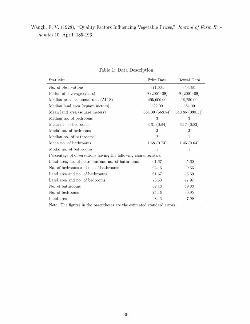
Waugh, F. V. (1928), “Quality Factors Influencing Vegetable Prices,” Journal of Farm Eco-

nomics 10, April, 185-196.

Table 1: Data Description

Statistics Price Data Rental Data

No. of observations 371,604 358,381

Period of coverage (years) 9 (2001–09) 9 (2001–09)

Median price or annual rent (AU $) 495,000.00 18,250.00

Median land area (square meters) 592.00 584.00

Mean land area (square meters) 684.39 (568.54) 640.86 (390.11)

Median no. of bedrooms 3 3

Mean no. of bedrooms 3.31 (0.84) 3.17 (0.82)

Modal no. of bedrooms 3 3

Median no. of bathrooms 2 1

Mean no. of bathrooms 1.68 (0.74) 1.45 (0.64)

Modal no. of bathrooms 1 1

Percentage of observations having the following characteristics:

Land area, no. of bedrooms and no. of bathrooms 61.67 45.60

No. of bedrooms and no. of bathrooms 62.43 49.33

Land area and no. of bathrooms 61.67 45.60

Land area and no. of bedrooms 73.50 47.97

No. of bathrooms 62.43 49.33

No. of bedrooms 74.46 99.95

Land area 98.43 47.99

Note: The figures in the parentheses are the estimated standard errors.

36

Table 2: Distributions of Characteristics in the Price and Rental Data (in %)

Characteristics Data Counts

1 2 3 4 5 6 Total

Bedrooms Price 0.62 13.30 49.40 29.22 6.48 0.98 100.00

Rent 1.52 15.48 53.22 23.79 5.88 0.11 100.00

Bathrooms Price 46.74 40.07 11.61 1.40 0.18 n.a. 100.00

Rent 61.74 31.54 6.20 0.48 0.03 n.a. 100.00

Characteristics Data Deciles

1st 2nd 3rd 4th 5th 6th 7th 8th 9th 10th

Land Area∗ Price 9.10 10.01 9.99 10.95 9.50 9.97 10.55 9.91 10.19 9.83

Rent 11.93 10.17 10.15 9.61 9.44 10.03 9.39 9.67 9.54 10.07

Postcodes Price 17.62 14.91 11.79 8.30 9.66 8.28 8.97 8.09 7.33 5.04

(by Price)† Rent 20.40 15.73 12.35 7.16 8.98 8.09 7.97 7.65 7.15 4.52

Postcodes Price 18.56 15.46 9.31 7.60 10.96 9.40 9.22 7.91 6.46 5.11

(by Rent)§ Rent 19.98 16.97 10.07 7.27 10.55 8.58 8.46 7.69 5.92 4.50

∗The price and rental data are pooled before dividing them into deciles in terms of land area.Therefore, each decile corresponds to the same land area in both data sets.†Houses are ordered from the cheapest to the most expensive in terms of price.§Houses are ordered from the cheapest to the most expensive in terms of rent.

Table 3: HM1 Regression Results

Statistics Price Models Rent Models

No. of observations 25462 (12273) 18157 (16235)

No. of parameters 204 (17) 204 (17)

Adjusted R2 (%) 78.35 (3.29) 79.33 (1.95)

Location attributes: Joint contribution (%) 54.9 (2.89) 48.08 (1.94)

% of significant coefficients 93.26 (2.10) 85.77 (7.53)

Temporal attributes: Joint contribution (%) 0.32 (0.33) 0.13 (0.11)

% of significant coefficients 96.30 (11.11) 55.56 (52.70)

Physical attributes: Joint contribution (%) 9.60 (0.93) 12.74 (3.76)

% of significant coefficients 84.13 (8.58) 68.25 (8.07)

Note: The numbers are the mean results obtained from the 9 yearly regressions.The numbers in parentheses are the standard deviations of the 9 yearly regressions,indicating how stable or dispersed the statistics are across yearly regressions. Thejoint contribution is calculated by taking the difference in the adjusted R2 betweenthe unrestricted and restricted models. The statistical tests are conducted at the5% significance level.

37

Table 4: HM2–HM8 Regression Results

Statistics Data HM2 HM3 HM4 HM5 HM6 HM7 HM8

Adjusted R2 (in %) Price 75.92 76.67 74.90 74.19 72.36 67.06 63.87

(4.55) (2.71) (3.65) (3.86) (5.09) (2.87) (4.26)

Rent 78.54 74.44 75.18 73.97 72.50 65.85 62.83

(2.15) (1.10) (1.96) (0.95) (2.40) (1.74) (0.95)

% of coefficients having Price 92.29 98.76 99.20 92.26 91.15 97.32 90.33

the same sign as HM1 (5.43) (1.17) (6.64) (5.18) (6.06) (1.81) (4.34)

Rent 97.44 95.80 97.04 95.52 92.48 91.37 87.16

(2.15) (1.49) (1.99) (1.89) (4.35) (2.96) (3.06)

Notes: (1) The numbers are the mean results obtained from the 9 yearly regressions.The numbers in parentheses are the standard deviations of the 9 yearly regressions.(2) HM1–HM8 regressions include the following physical characteristics and theirinteraction terms. HM1: bed, bath, land; HM2: bed, bath; HM3: bath, land;HM4: bed, land; HM5: bath; HM6: bed; HM7: land; HM8: no physical characteristics.

Table 5: Omitted Variables Adjustment Factors: λt,HM8 and λt,HMj|HM8

Year λt,HM8 λt,HMj|HM8, j = 1, . . . , 8

HM1 HM2 HM3 HM4 HM5 HM6 HM7 HM8

2001 1.160 0.943 0.946 0.944 0.981 0.944 0.981 0.989 1.000

2002 1.169 0.948 0.951 0.947 0.980 0.948 0.987 0.993 1.000

2003 1.120 0.943 0.945 0.944 0.977 0.948 0.981 0.993 1.000

2004 1.115 0.939 0.953 0.939 0.975 0.953 0.987 0.992 1.000

2005 1.103 0.962 0.967 0.960 0.987 0.962 0.992 0.999 1.000

2006 1.121 0.960 0.963 0.962 0.987 0.963 0.991 0.995 1.000

2007 1.117 0.954 0.949 0.966 0.975 0.960 0.974 1.002 1.000

2008 1.084 0.956 0.956 0.966 0.973 0.964 0.976 1.005 1.000

2009 1.052 0.965 0.960 0.972 0.980 0.968 0.984 1.004 1.000

Average 1.115 0.952 0.954 0.955 0.979 0.957 0.984 0.997 1.000

Note: Overall adjustment factor: λt,HMj = λt,HM8 × λt,HMj|HM8. Forexample, λ2001,HM1 = 1.160× 0.943 = 1.094.

38

Table 6: Actual and Quality-Adjusted Median Price-Rent Ratios and Quality Bias

Year Actual Quality Quality Bias 1 (%) Bias 2 (%)

Unadjusted Adjusted 1 Adjusted 2

2001 25.63 23.20 20.48 10.46 25.15

2002 30.42 28.10 24.29 8.24 25.24

2003 34.72 32.03 28.59 8.38 21.45

2004 35.48 32.33 29.78 9.74 19.13

2005 33.41 29.55 27.09 13.11 23.32

2006 32.06 27.79 25.44 15.36 26.01

2007 27.45 25.13 23.60 9.23 16.33

2008 23.01 22.22 21.40 3.55 7.52

2009 21.85 22.13 21.62 -1.26 1.10

Average 29.34 26.96 24.70 8.70 18.36

Notes: (1) The quality-adjusted 1 series is calculated from (14). It qualityadjusts based on the characteristics available in our data set. The quality-adjusted 2 series also accounts for missing characteristics in some of ourhedonic models and omitted variables (with the latter adjustments madewith reference to the subset of dwellings in our data set that both selland rent). (2) Bias k = 100 × [(Actual/Quality-adjusted k) - 1].

Table 7: A Comparison of Equilibrium and Actual Price-Rent Ratios

Year rt gt − πet Equilibrium Pt/Rt Actual Pt/Rt Implied gt − πe

t

x=10 x=20 x=30 x=10 x=20 x=30 Adjust Unadj. Adjust Unadj.

2001 0.056 0.029 0.024 0.024 19.18 17.39 17.64 20.48 25.63 0.032 0.042

2002 0.058 0.045 0.037 0.028 26.11 21.45 18.10 24.29 30.42 0.042 0.050

2003 0.054 0.060 0.047 0.031 52.88 32.02 21.10 28.59 34.72 0.044 0.050

2004 0.056 0.062 0.048 0.033 52.97 30.33 20.92 29.78 35.48 0.047 0.053

2005 0.053 0.059 0.047 0.033 47.57 29.89 21.94 27.09 33.41 0.041 0.048

2006 0.056 0.056 0.043 0.033 38.47 27.06 21.03 25.44 32.06 0.042 0.050

2007 0.060 0.053 0.045 0.036 32.41 25.50 20.29 23.60 27.45 0.043 0.048

2008 0.058 0.048 0.042 0.033 24.66 19.79 20.25 21.40 23.01 0.036 0.039

2009 0.050 0.034 0.018 0.030 26.14 19.47 22.40 21.62 21.85 0.029 0.029

Mean 0.056 0.049 0.038 0.031 35.60 24.77 20.41 24.72 29.34 0.040 0.046

Notes: ωt = 0.01, δt = 0.025, γt = 0.02 and πet = 0.03 for the entire period.

39

Table 8: Cross-Sectional Variation of Price-Rent Ratios

2001 2002 2003 2004 2005 2006 2007 2008 2009 Pooled

Elasticity of price-rent ratio to changes in price or rent:∗

∆ in price 0.213 0.200 0.181 0.140 0.134 0.145 0.188 0.211 0.213 0.206(0.001) (0.001) (0.002) (0.002) (0.002) (0.001) (0.001) (0.001) (0.001) (0.001)

∆ in rent 0.201 0.171 0.100 0.077 0.106 0.144 0.187 0.209 0.225 0.111(0.002) (0.002) (0.002) (0.002) (0.002) (0.002) (0.001) (0.001) (0.001) (0.001)

Notes: ∗The figures are the estimated slope coefficients obtained when the log of the quality-adjustedprice-rent ratios are regressed on an intercept and the log of price or the log of rent. The figures in thebrackets are the estimated standard errors.

Table 9: Quality-Adjusted Price-Rent Ratios for Different Market Segments

Houses are ordered from cheapest to most expensive

Year Price-Rent from Price Data Price-Rent From Rent Data

Lower Median Upper Lower Median UpperQuartile Quartile Quartile Quartile

2001 19.28 21.89 22.63 18.49 20.09 21.82

2002 21.17 24.79 26.98 21.72 24.20 25.96

2003 27.39 29.17 31.47 26.27 28.91 30.16

2004 28.61 30.11 30.91 28.35 29.99 30.14

2005 26.52 27.07 27.35 26.14 27.36 28.19

2006 23.88 26.02 29.40 23.67 24.93 25.84

2007 21.57 25.65 25.54 21.24 23.01 25.66

2008 19.70 21.07 24.08 19.47 21.26 23.58

2009 19.82 21.36 26.13 19.36 21.27 23.81

Average 23.10 25.24 27.17 22.75 24.56 26.13

40

Table 10: Robustness Checks

Year Median Price-rent Ratios Obtained from Different Methods

Base (a) (b) (c) (d) (e) (f) (g) (h)

2001 20.48 23.35 21.10 20.76 21.05 21.35 20.69 20.08 20.66

2002 24.29 28.19 25.47 24.55 24.52 24.92 24.53 23.98 24.29

2003 28.59 31.81 29.68 28.82 28.51 28.96 29.04 28.66 28.66

2004 29.78 32.11 30.38 29.90 29.10 29.96 30.05 29.53 29.96

2005 27.09 29.48 28.08 26.98 26.94 27.28 27.43 26.37 27.11

2006 25.44 27.76 26.21 25.36 25.89 25.63 25.51 24.84 25.44

2007 23.60 25.31 24.56 23.61 23.65 23.63 23.41 23.35 23.57

2008 21.40 22.47 22.06 21.54 21.88 21.22 21.27 21.11 21.42

2009 21.62 22.46 22.44 21.76 21.31 21.17 21.51 21.34 21.64

Average 24.70 27.00 25.55 24.81 24.76 24.90 24.83 24.36 24.75

Notes: (a) Obtained from running HM1 models on observations which have all three physicalcharacteristics, without correcting for omitted variables bias. (b) Single imputation price-rentratios—P/R(sold)SI

th and P/R(rented)SItj (see section 1.2)—are estimated, instead of double

imputation price-rent ratios. (c) Hedonic models in equations 6 and 7 are specified on priceand rent levels instead of log of prices and rents. (d) Med[P/RDI

pooled] specified in section 1.3is used. (e) Double imputation hedonic price and rent indexes are used in order to estimatePst and Rst in equations 16 and 15, respectively (the main results use repeat-sales and -rentsindexes). (f) For dwellings with multiple prices and rents, we consider each price-rent pair in orderto obtain P/RAM

t (in equation 17) where the main results use only the chronologically closestprice and rent observations. (g) The regressions required to obtain λt,HM8 (equation 18) areestimated using the sample HM8s\AMs (instead of using HM8s which includes AMs) and then theprice-rent ratios of the AMS dwellings are imputed from the regression results. (h) The correctionfactor (λt,HMj|HM8 equation 19) is obtained using the HM1s, i.e. λt,HMj|HM8

= HMjm(HM1s)/HM8m(HM1s).

41

Figure 1: Quality-Adjusted and Unadjusted Price-Rent Ratios

2001 2002 2003 2004 2005 2006 2007 2008 200918

20

22

24

26

28

30

32

34

36

Price

−R

en

t R

atio

s

Year

Quality−unadjusted price−rent ratios(simple median price to median rent ratios)

Quality−adjusted, but not missing and omittedcharacteristics bias corrected, price−rent ratios

Quailty−adjusted, and missing and omittedcharacteristics bias corrected price−rent ratios

Figure 2: Price and Rent Indexes of Lower and Upper Ends of the Market

2001 2002 2003 2004 2005 2006 2007 2008 20090.9

1

1.1

1.2

1.3

1.4

1.5

1.6

1.7

Ind

ex

(a) Hedonic Price

2001 2002 2003 2004 2005 2006 2007 2008 20090.9

1

1.1

1.2

1.3

1.4

1.5

1.6

1.7

(b) Repeat−sales

2001 2002 2003 2004 2005 2006 2007 2008 20090.9

1

1.1

1.2

1.3

1.4

1.5

1.6

1.7

(c) Median Price

2001 2002 2003 2004 2005 2006 2007 2008 20090.9

1

1.1

1.2

1.3

1.4

1.5

1.6

1.7

Year

Ind

ex

(d) Hedonic Rent

2001 2002 2003 2004 2005 2006 2007 2008 20090.9

1

1.1

1.2

1.3

1.4

1.5

1.6

1.7

Year

(e) Repeat−rents

2001 2002 2003 2004 2005 2006 2007 2008 20090.9

1

1.1

1.2

1.3

1.4

1.5

1.6

1.7

Year

(f) Median Rent

Lower Upper All

42

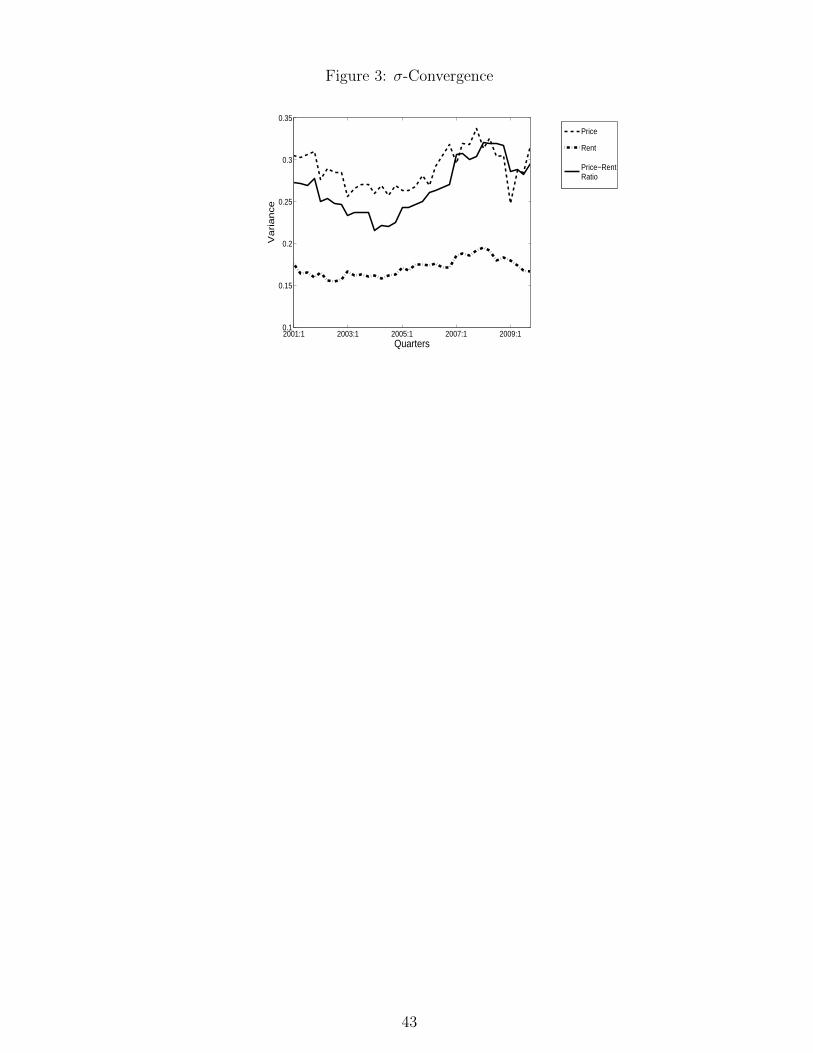
Figure 3: σ-Convergence

2001:1 2003:1 2005:1 2007:1 2009:10.1

0.15

0.2

0.25

0.3

0.35

Va

ria

nce

Quarters

Price

Rent

Price−RentRatio

43