heckscher-ohlin: evidence from virtual trade in value added · 2015-08-12 · heckscher-ohlin:...

Heckscher-Ohlin:Evidence from virtual trade in value added∗

Tadashi Ito†

Lorenzo Rotunno‡

Pierre-Louis Vezina§

July 15, 2015

Abstract

The fragmentation of production chains across borders is one of the most distinctivefeature of the last 30 years of globalization. Nonetheless, our understanding of itsimplications for trade theory and policy is only in its infancy. We suggest that trade invalue added should follow theories of comparative advantage more closely than grosstrade, as value-added flows capture where factors of production, e.g. labor and capital,are used along the global value chain. We find empirical evidence that Heckscher-Ohlintheory does predict manufacturing trade in value-added, and it does so better than forgross shipment flows. While countries exports across a broad range of sectors, theyspecialize in techniques using their abundant factor intensively.

JEL CODES: F13Key Words: Heckscher-Ohlin, value added, trade theory

∗We are grateful to seminar participants at Osaka University, IDE-JETRO Bangkok, DEGIT Geneva,and at the Bari superconference.†IDE-JETRO Tokyo, Japan. Email: tadashi [email protected]‡University of Oxford. UK. Email: [email protected]§King’s College London. UK. Email: [email protected]

1 INTRODUCTION

The second unbundling, or the fragmentation of production chains across borders, is one of

the most distinctive feature of the last 30 years of globalization (Baldwin, 2011). Nonetheless,

our understanding of its implications for trade theory and policy is only in its infancy. One

explanation for this delay is the only-recent release of input-output matrices that cover the

whole world and allow for a better understanding of the location of production across global

value chains.

One implication of global value chains is that ‘Made in China’ no longer means ‘Made

in China’. Koopman et al. (2008) estimate that the share of domestic content in China

exports is about 50%. One recurring example is that of Apple’s iPad, ‘Made in China’ but

with Chinese labor accounting for only about 3% of its value added. Gross trade figures,

e.g. Chinese exports of iPads, are hence no perfect guide to understand where value addition

occurs. They also imply a ‘double-counting’ of value added, as the value added embedded

in parts and components is counted when both intermediates and final goods cross borders.

The ‘double-counting’ means that trade data overstates the domestic value-added content of

exports (see Figure 1).

Economists have thus recently focused on capturing the value-added content of trade

Johnson and Noguera (2012) and the World Trade Organization launched a ’Made in the

World’ initiative to encourage research on the topic. Extracting the value-added embedded

in exports allow us to trace where factors of production are used. For example, it allows us

to identify that China’s electronics exports embed wages paid to Chinese labor and profits

pocketed by US wholesalers. It elucidates the paradox that labor-abundant China apparently

exports capital-intensive and sophisticated products. When looking at trade in value added,

we find that China actually exports only unskilled labor embedded in iPads. Another

example is that of Boeing’s Dreamliner. While is is ‘Made in the USA’, it embeds value

from a long list of countries (Figure 2).

2

We suggest that trade in value added should follow theories of comparative advantage

more closely than gross trade. The reason is that it tells you where factors of production, e.g.

labor and capital, are used. As Daudin et al. (2011) notes, only a value-added trade measure

can answer the question who produces for whom in the world economy?’. Value-added trade

thus offers a new lens to test for theories of comparative advantage. Do labor-abundant

countries export labor-intensive products? Or rather, do labor-abundant countries export

labor-intensive value-added? Previous tests of comparative advantage theories based on facto

endowments include Romalis (2004), who shows that the US imports more skill-intensive

products from skill-abundant countries, Chor (2010) who explains industry trade flows using

Heckscher-Ohlin and other sources of comparative advantage, and Trefler and Zhu (2010),

who tests for factor content predictions in the presence of traded intermediates.

In this paper we combine Chor (2010) and Johnson and Noguera (2012) to provide a

new test for Heckscher-Ohlin theory. The Heckscher-Ohlin prediction is that countries will

export goods whose production uses its abundant factor intensively. Does Japan export

more skill-intensive value added than labor-abundant countries? Our prediction is that

the value-added trade patterns fit the Heckscher-Ohlin predictions better than gross trade

patterns as they capture precisely the location of production factors. We mimic the regression

setting of Chor (2010), who tested for theories of comparative advantage, but including

value-added trade rather than gross trade data on the left-hand side. In doing so we

generalize the approach of Davis and Weinstein (2001), Trefler and Zhu (2010) and others to

test for Heckscher-Ohlin predictions to a framework with bilateral trade costs. We thus add

to a resurgence of papers that decompose the factor content of trade to test Heckscher-Ohlin

theory, e.g. Egger et al. (2011) and Fisher (2011) who show that it is important to take into

account international differences in technology (see Figure 10), which depends largely on

labor requirements across countries (Nishioka, 2012). Our paper is also in line with Fisher

and Marshall (2013) who insist that the factor content of trade in labor is not an exchange

of person-years, but trade in value added attributed to a worker.

3

We find empirical evidence that HO theory does predict manufacturing trade in value-added,

and it does so better than for gross shipment flows.

The paper proceeds as follows. In the next section we describe the data and present our

empirical strategy. A third section presents the results and a fourth concludes.

2 DATA AND EMPIRICAL STRATEGY

We use data from the World Input-Output Database (WIOD). It provides international

input-output tables for 40 countries (Figure 4), 34 sectors, from 1995 to 2009 (Timmer,

2012). This data allows us to compute the value added embedded in final imports as the

sale value of a product equals to the cost of intermediate inputs plus value added. Here value

added refers to the cost of primary inputs such as labor as well as profits. For example we

can identify where the workers involved into Chinese electronics were employed, by sector

and by nation. It would most likely involve skilled labor in the US who designed and market

the product, as well as workers in Taiwan that produced the parts and components, as well

as other inputs from the chemical and metal industries in other countries. By tracking down

the whole process until the sales value equals the sum of value added, we can trace the value

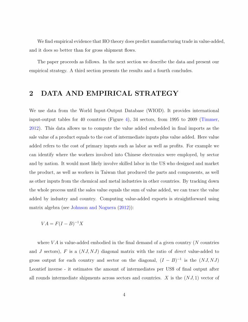
added by industry and country. Computing value-added exports is straightforward using

matrix algebra (see Johnson and Noguera (2012)):

V A = F (I −B)−1X

where V A is value-added embodied in the final demand of a given country (N countries

and J sectors), F is a (NJ,NJ) diagonal matrix with the ratio of direct value-added to

gross output for each country and sector on the diagonal, (I − B)−1 is the (NJ,NJ)

Leontief inverse - it estimates the amount of intermediates per US$ of final output after

all rounds intermediate shipments across sectors and countries. X is the (NJ, 1) vector of

4

gross shipments for final demand, i.e. the destination country.

Trade in value added may be direct (embodied in bilateral gross trade shipments) or

indirect (traveling through intermediate shipments that cross multiple borders). See Figure

3. We label the total value added trade as ‘Virtual VA trade’.

Figure 5 provides a network view of trade in value added and in gross terms. One clear

observation is that the contribution of China in global value-added trade is smaller than in

gross terms. This is also seen in Figure 6 which shows the difference between the two flows is

even bigger in China’s exports to Asia, as many of those are parts that will be re-exported to

the US or EU and thus embedded in China’s value-added exports to the US and EU. Figure

7 shows that China’s top export sectors in value-added terms are different from those in

gross terms. While electric equipment remains on top, plastics, transport equipment (cars),

and leather fall out of the top 10. One explanation is that most of the leather exported

from China embeds value added in Ethiopia for example, and plastic exports embed oil from

Indonesia. Mining and agriculture enter the top 10 in value-added terms. This may be

because China doesn’t export its mining products, such as rare earths, but rather embeds

them in electronic exports. Yet they account for a large share of value-added exported.

Figures 8 and 9 similarly display the case of Japan exports. Here we note that Japan’s

value-added exports to the US and EU are larger, not smaller, than its gross exports. This

may be because of the Japanese value-added embedded in China’s and other Southeast Asian

countries exports of electronics. Note also that services such as finance, inland transport,

and wholesale do not appear as top-10 gross exports but do make the list for value-added

exports as they are embedded in Japan’s sophisticated exports.

WIOD also provides data on factor use and payments - three types of labor (high-skilled,

medium-skilled and low-skilled) and capital. We follow (Timmer et al., 2014) and merge the

low and medium categories in an ‘unskilled’ aggregate. The factors are Labor (L), Unskilled

labor (LUS) and High-skilled labor (LHS). We leave physical capital aside as it is constructed

as a residual and is thus not as precisely-measured as human capital endowments.

5

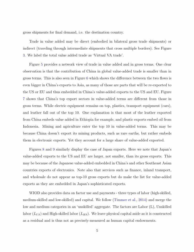
We regress virtual VA exports and gross exports on relative endowments interacted with

relative intensities. Formally, we estimate the following model:

ln(V A)ijkt = αikt + σjt + β1 ln(lhslus

)jkt + β2 ln(lhslus

)jkt × ln(Lhs

Lus

)jt + εijkt

where αikt and σjt are importer-industry-year and exporter-year fixed effects. L is for

labor. Lower-case letters are for intensities, upper-case endowments. Our prediction is that

β2 is positive and significant, even more so for value-added exports than for gross exports.

3 RESULTS

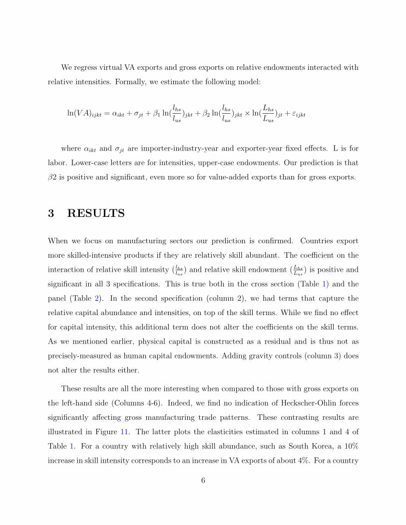
When we focus on manufacturing sectors our prediction is confirmed. Countries export

more skilled-intensive products if they are relatively skill abundant. The coefficient on the

interaction of relative skill intensity ( lhslus

) and relative skill endowment (Lhs

Lus) is positive and

significant in all 3 specifications. This is true both in the cross section (Table 1) and the

panel (Table 2). In the second specification (column 2), we had terms that capture the

relative capital abundance and intensities, on top of the skill terms. While we find no effect

for capital intensity, this additional term does not alter the coefficients on the skill terms.

As we mentioned earlier, physical capital is constructed as a residual and is thus not as

precisely-measured as human capital endowments. Adding gravity controls (column 3) does

not alter the results either.

These results are all the more interesting when compared to those with gross exports on

the left-hand side (Columns 4-6). Indeed, we find no indication of Heckscher-Ohlin forces

significantly affecting gross manufacturing trade patterns. These contrasting results are

illustrated in Figure 11. The latter plots the elasticities estimated in columns 1 and 4 of

Table 1. For a country with relatively high skill abundance, such as South Korea, a 10%

increase in skill intensity corresponds to an increase in VA exports of about 4%. For a country

6

with relative skill scarcity, such as India, a 10% increase in skill intensity corresponds to a

decrease in VA exports of about 5%. This is exactly in line with countries exporting along

their comparative advantage. When looking at gross exports, we do not find such clearly

differing elasticities at the opposite end of the skill abundance distribution.

When looking at services and total trade (Tables 3 4 5 6) we find no significant difference

between gross and virtual VA flows. This is illustrated in Figure 12. While the results

still lean more in favor of Heckscher-Ohlin forces when looking at services in value-added

terms, we find no significant difference between the 2 types of flows. This difference between

services and manufacturing may be explained by the fact that is it mostly in manufacturing

that global value chains have emerged.

4 CONCLUSION

Tests of the Heckscher-Ohlin theory have come a long way since Leontief’s paradox, i.e.

the observation in 1953 that the US, a capital abundant country, was importing mostly

capital-intensive goods, and since Bowen et al. (1987) claimed that net factor exports are no

better predicted by measured factor abundance than by a coin flip. While many studies have

followed and claimed that the theory performed badly empirically, we find empirical evidence

that it does predict manufacturing trade in value-added, and it does so better than for gross

shipment flows. Countries exports ’value’ that they produce using their abundant factor

intensively. As Nishioka (2012) noted, the bulk of world factor content of trade does not

arise from specialization across goods, but rather via specialization in abundance-inspired

techniques. One note of caution is that when we look at total trade, we do not find any

statistical difference between VA and gross flows. This may be because global value chains

are still mostly national. The spread of global value chains should make HO theory more,

rather than less,relevant.

7

References

Baldwin, R., 2011. Trade And Industrialisation After Globalisation’s 2nd Unbundling: How

Building And Joining A Supply Chain Are Different And Why It Matters. NBER Working

Papers 17716. National Bureau of Economic Research, Inc.

Bowen, H.P., Leamer, E.E., Sveikauskas, L., 1987. Multicountry, Multifactor Tests of the

Factor Abundance Theory. American Economic Review 77(5), 791–809.

Chor, D., 2010. Unpacking sources of comparative advantage: A quantitative approach.

Journal of International Economics 82(2), 152–167.

Daudin, G., Rifflart, C., Schweisguth, D., 2011. Who produces for whom in the world

economy? Canadian Journal of Economics 44(4), 1403–1437.

Davis, D.R., Weinstein, D.E., 2001. An Account of Global Factor Trade. American Economic

Review 91(5), 1423–1453.

Egger, P., Marshall, K.G., Fisher, E.O., 2011. Empirical foundations for the resurrection of

Heckscher-Ohlin theory. International Review of Economics & Finance 20(2), 146–156.

Fisher, E., Marshall, K.G., 2013. Testing the heckscher-ohlin-vanek paradigm in a world

with cheap foreign labor. Unpublished manuscript .

Fisher, E.O., 2011. Heckscher-Ohlin theory when countries have different technologies.

International Review of Economics & Finance 20(2), 202–210.

Johnson, R.C., Noguera, G., 2012. Accounting for intermediates: Production sharing and

trade in value added. Journal of International Economics 86(2), 224–236.

Koopman, R., Wang, Z., Wei, S.J., 2008. How Much of Chinese Exports is Really Made In

China? Assessing Domestic Value-Added When Processing Trade is Pervasive. Working

Paper 14109. National Bureau of Economic Research.

8

Nishioka, S., 2012. International differences in production techniques: Implications for the

factor content of trade. Journal of International Economics 87(1), 98–104.

Romalis, J., 2004. Factor Proportions and the Structure of Commodity Trade. American

Economic Review 94(1), 67–97.

Timmer, M.P., 2012. The World Input-Output Database (WIOD): Contents, Sources and

Methods. Technical Report. WIOD Working Paper Number 10.

Timmer, M.P., Erumban, A.A., Los, B., Stehrer, R., de Vries, G.J., 2014. Slicing Up Global

Value Chains. Journal of Economic Perspectives 28(2), 99–118.

Trefler, D., Zhu, S.C., 2010. The structure of factor content predictions. Journal of

International Economics 82(2), 195–207.

9

Table 1: Manufacturing trade - Cross-section

(1) (2) (3) (4) (5) (6)

Virtual VA Gross exports

ln(

lhslus

)× ln

(Lhs

Lus

)0.309*** 0.339*** 0.339*** 0.167 0.159 0.159

(0.0800) (0.0918) (0.0945) (0.112) (0.129) (0.132)

ln(

lhslus

)0.642*** 0.560*** 0.560** 0.222 0.109 0.109

(0.209) (0.215) (0.221) (0.266) (0.283) (0.290)

ln(

klus

)× ln

(KLus

)-0.00931 -0.00931 0.0155 0.0155

(0.0297) (0.0302) (0.0335) (0.0344)

ln(

klus

)0.272** 0.272** 0.137 0.137

(0.125) (0.127) (0.138) (0.142)

Log(distance) -0.717*** -0.981***

(0.0508) (0.0678)

Same cty 2.029*** 2.186***

(0.195) (0.238)

Share border 0.490*** 0.655***

(0.0918) (0.113)

Common lang 0.0300 0.0501

(0.0918) (0.110)

Colony 0.158* 0.302***

(0.0891) (0.110)

Legal 0.187*** 0.256***

(0.0432) (0.0510)

FTA 0.393*** 0.506***

(0.0919) (0.123)

Obs 25,520 25,520 25,520 25,520 25,520 25,520

R2 0.671 0.674 0.854 0.575 0.577 0.807

All regressions include importer-industry and exporter dummies. Two-way clustered standard errors by

exporter-industry and country-pair are in parenthesis. Significant at: *10%, **5%, ***1% level.

10

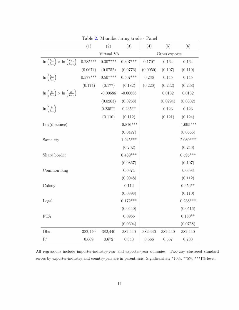
Table 2: Manufacturing trade - Panel

(1) (2) (3) (4) (5) (6)


ln(

lhslus

)× ln

(Lhs

Lus

)0.285*** 0.307*** 0.307*** 0.170* 0.164 0.164

(0.0674) (0.0752) (0.0776) (0.0950) (0.107) (0.110)

ln(

lhslus

)0.577*** 0.507*** 0.507*** 0.236 0.145 0.145

(0.174) (0.177) (0.182) (0.220) (0.232) (0.238)

ln(

klus

)× ln

(KLus

)-0.00686 -0.00686 0.0132 0.0132

(0.0263) (0.0268) (0.0294) (0.0302)

ln(

klus

)0.235** 0.235** 0.123 0.123

(0.110) (0.112) (0.121) (0.124)

Log(distance) -0.816*** -1.095***

(0.0427) (0.0566)

Same cty 1.945*** 2.080***

(0.202) (0.246)

Share border 0.439*** 0.595***

(0.0867) (0.107)


(0.0948) (0.112)

Colony 0.112 0.252**

(0.0898) (0.110)

Legal 0.172*** 0.238***

(0.0440) (0.0516)

FTA 0.0966 0.180**

(0.0604) (0.0758)

Obs 382,440 382,440 382,440 382,440 382,440 382,440

R2 0.669 0.672 0.843 0.566 0.567 0.783

All regressions include importer-industry-year and exporter-year dummies. Two-way clustered standard

errors by exporter-industry and country-pair are in parenthesis. Significant at: *10%, **5%, ***1% level.

11

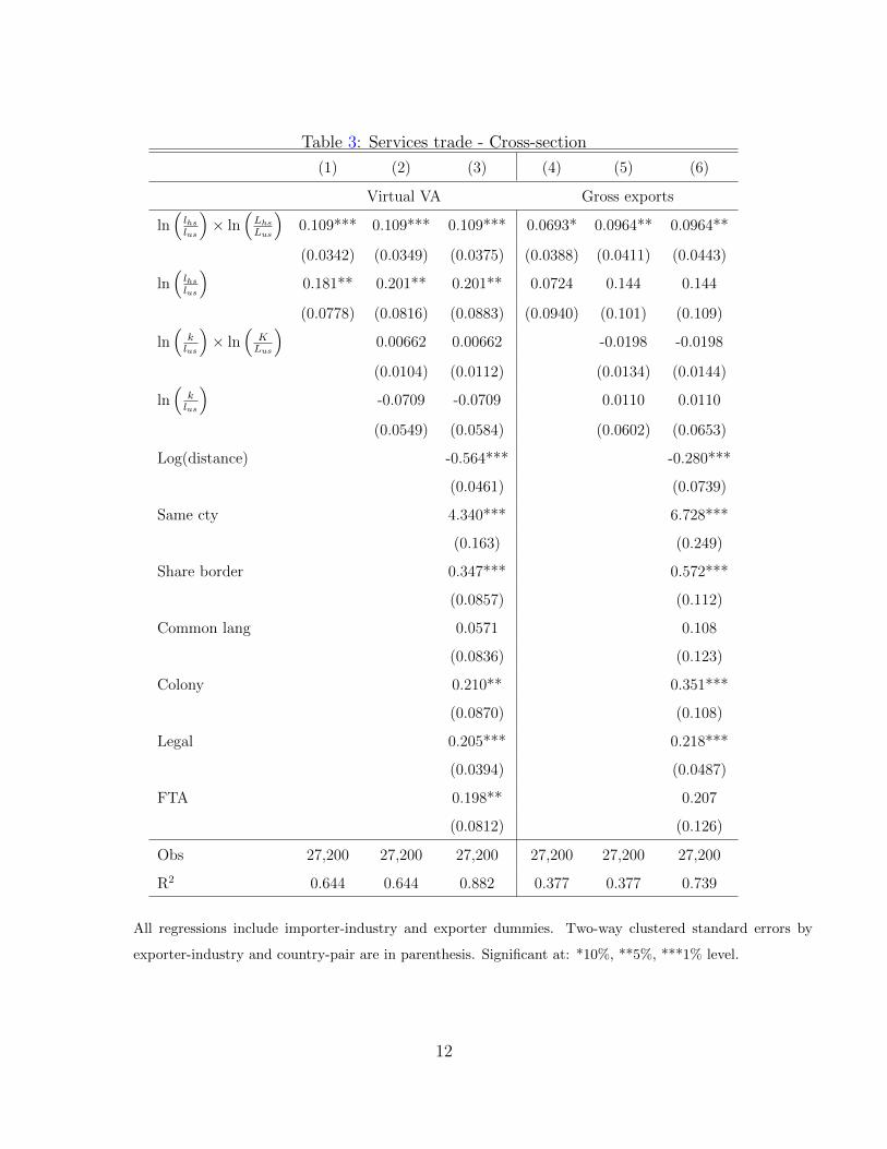
Table 3: Services trade - Cross-section

(1) (2) (3) (4) (5) (6)


ln(

lhslus

)× ln

(Lhs

Lus

)0.109*** 0.109*** 0.109*** 0.0693* 0.0964** 0.0964**

(0.0342) (0.0349) (0.0375) (0.0388) (0.0411) (0.0443)

ln(

lhslus

)0.181** 0.201** 0.201** 0.0724 0.144 0.144

(0.0778) (0.0816) (0.0883) (0.0940) (0.101) (0.109)

ln(

klus

)× ln

(KLus

)0.00662 0.00662 -0.0198 -0.0198

(0.0104) (0.0112) (0.0134) (0.0144)

ln(

klus

)-0.0709 -0.0709 0.0110 0.0110

(0.0549) (0.0584) (0.0602) (0.0653)

Log(distance) -0.564*** -0.280***

(0.0461) (0.0739)

Same cty 4.340*** 6.728***

(0.163) (0.249)

Share border 0.347*** 0.572***

(0.0857) (0.112)


(0.0836) (0.123)

Colony 0.210** 0.351***

(0.0870) (0.108)

Legal 0.205*** 0.218***

(0.0394) (0.0487)

FTA 0.198** 0.207

(0.0812) (0.126)

Obs 27,200 27,200 27,200 27,200 27,200 27,200

R2 0.644 0.644 0.882 0.377 0.377 0.739



12

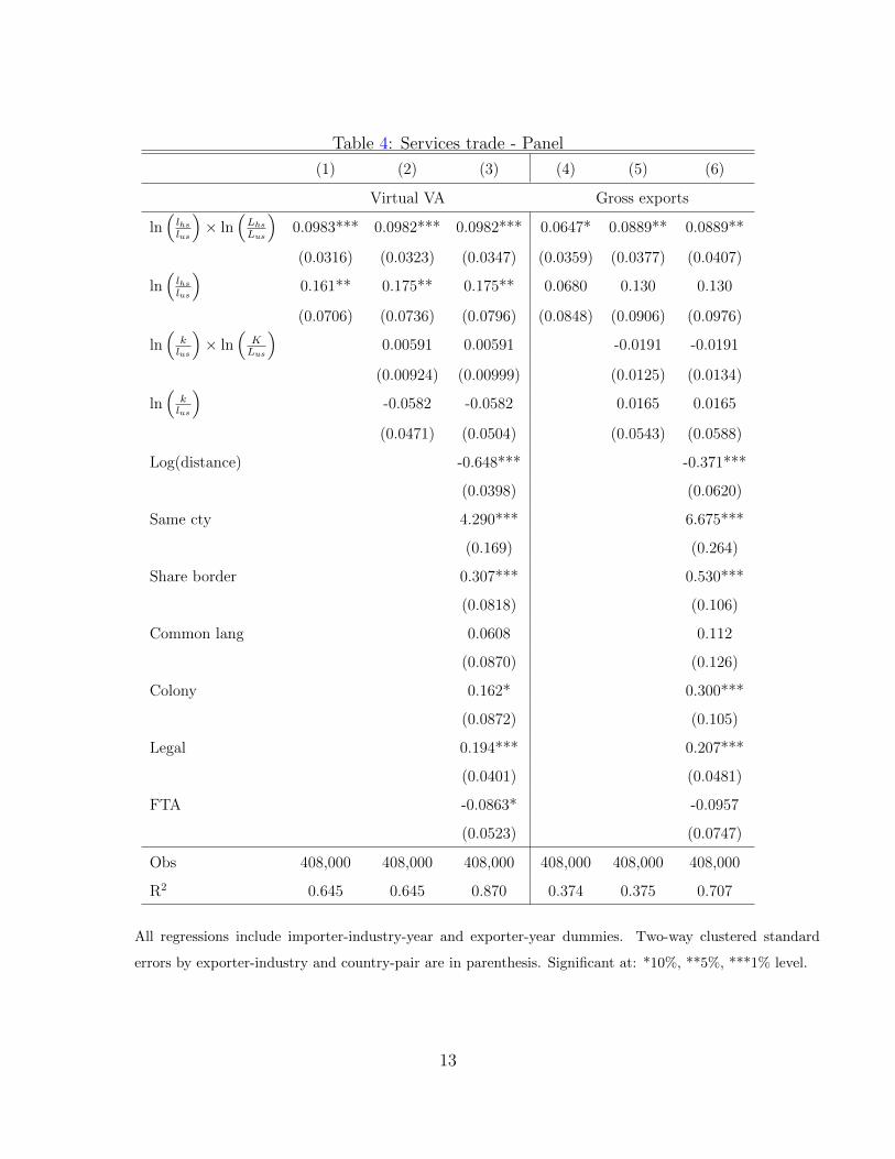
Table 4: Services trade - Panel

(1) (2) (3) (4) (5) (6)


ln(

lhslus

)× ln

(Lhs

Lus

)0.0983*** 0.0982*** 0.0982*** 0.0647* 0.0889** 0.0889**

(0.0316) (0.0323) (0.0347) (0.0359) (0.0377) (0.0407)

ln(

lhslus

)0.161** 0.175** 0.175** 0.0680 0.130 0.130

(0.0706) (0.0736) (0.0796) (0.0848) (0.0906) (0.0976)

ln(

klus

)× ln

(KLus

)0.00591 0.00591 -0.0191 -0.0191

(0.00924) (0.00999) (0.0125) (0.0134)

ln(

klus

)-0.0582 -0.0582 0.0165 0.0165

(0.0471) (0.0504) (0.0543) (0.0588)

Log(distance) -0.648*** -0.371***

(0.0398) (0.0620)

Same cty 4.290*** 6.675***

(0.169) (0.264)

Share border 0.307*** 0.530***

(0.0818) (0.106)


(0.0870) (0.126)

Colony 0.162* 0.300***

(0.0872) (0.105)

Legal 0.194*** 0.207***

(0.0401) (0.0481)

FTA -0.0863* -0.0957

(0.0523) (0.0747)

Obs 408,000 408,000 408,000 408,000 408,000 408,000

R2 0.645 0.645 0.870 0.374 0.375 0.707



13

Table 5: Total trade - Cross-section

(1) (2) (3) (4) (5) (6)


ln(

lhslus

)× ln

(Lhs

Lus

)0.207*** 0.197*** 0.197*** 0.205*** 0.217*** 0.217***

(0.0301) (0.0321) (0.0335) (0.0392) (0.0417) (0.0433)

ln(

lhslus

)0.370*** 0.325*** 0.325*** 0.448*** 0.446*** 0.446***

(0.0768) (0.0798) (0.0833) (0.0970) (0.102) (0.106)

ln(

klus

)× ln

(KLus

)0.00321 0.00321 -0.0185 -0.0185

(0.0115) (0.0119) (0.0154) (0.0159)

ln(

klus

)0.0510 0.0510 0.108 0.108

(0.0544) (0.0563) (0.0668) (0.0692)

Log(distance) -0.638*** -0.620***

(0.0466) (0.0645)

Same cty 3.222*** 4.530***

(0.177) (0.215)

Share border 0.416*** 0.612***

(0.0877) (0.102)


(0.0861) (0.0949)

Colony 0.185** 0.328***

(0.0874) (0.0941)

Legal 0.196*** 0.237***

(0.0401) (0.0432)

FTA 0.292*** 0.352***

(0.0835) (0.112)

Obs 52,720 52,720 52,720 52,720 52,720 52,720

R2 0.653 0.653 0.859 0.503 0.504 0.757



14

Table 6: Total trade - Panel

(1) (2) (3) (4) (5) (6)


ln(

lhslus

)× ln

(Lhs

Lus

)0.189*** 0.180*** 0.180*** 0.182*** 0.193*** 0.193***

(0.0275) (0.0293) (0.0306) (0.0356) (0.0374) (0.0389)

ln(

lhslus

)0.329*** 0.288*** 0.288*** 0.388*** 0.384*** 0.384***

(0.0684) (0.0706) (0.0735) (0.0854) (0.0893) (0.0926)

ln(

klus

)× ln

(KLus

)0.00401 0.00401 -0.0164 -0.0164

(0.0103) (0.0107) (0.0142) (0.0147)

ln(

klus

)0.0444 0.0444 0.0992 0.0992

(0.0478) (0.0496) (0.0603) (0.0625)

Log(distance) -0.730*** -0.722***

(0.0398) (0.0538)

Same cty 3.155*** 4.451***

(0.184) (0.230)

Share border 0.371*** 0.561***

(0.0834) (0.0962)


(0.0895) (0.0988)

Colony 0.138 0.277***

(0.0879) (0.0931)

Legal 0.184*** 0.222***

(0.0410) (0.0436)

FTA 0.00189 0.0374

(0.0546) (0.0676)

Obs 790,440 790,440 790,440 790,440 790,440 790,440

R2 0.652 0.652 0.847 0.495 0.495 0.731



15

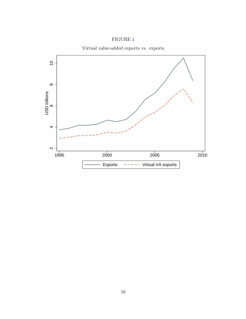
FIGURE 1

Virtual value-added exports vs. exports2

46

810

US

D tr

illio

ns

1995 2000 2005 2010

Exports Virtual VA exports

16

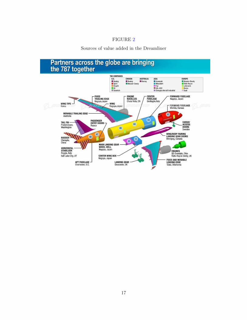
FIGURE 2

Sources of value added in the Dreamliner

17

FIGURE 3

Virtual trade in value added

18

FIG

UR

E4

Cou

ntr

yco

vera

ge

Virt

ual V

A e

xpor

ts /

GD

P

.47

.05

No

data

19

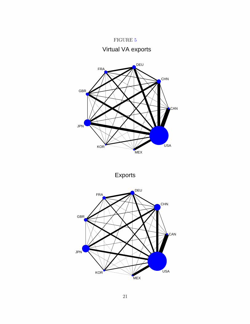
FIGURE 5

CAN

CHN

DEUFRA

GBR

JPN

KOR

MEX

USA

Virtual VA exports

CAN

CHN

DEUFRA

GBR

JPN

KOR

MEX

USA

Exports

21

FIGURE 6

China exports and virtual VA exports

5000

010

0000

1500

0020

0000

2500

0030

0000

$, m

illio

ns

1995 2000 2005 2010

VA exports Exports

China exports to Asia0

2000

0040

0000

6000

0080

0000

$, m

illio

ns

1995 2000 2005 2010

VA exports Exports

China exports to Europe and the Americas

22

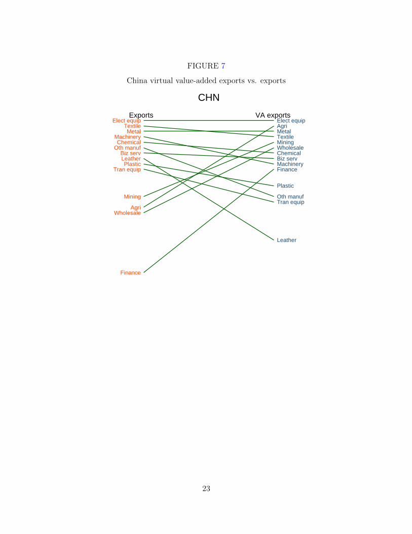
FIGURE 7

China virtual value-added exports vs. exports

Agri

Mining

Textile

Leather

Chemical

Plastic

MetalMachinery

Elect equip

Tran equip

Oth manuf

Wholesale

Finance

Biz serv

Agri

MiningTextile

Leather

Chemical

Plastic

Metal

Machinery

Elect equip

Tran equipOth manuf

Wholesale

Finance

Biz serv

Exports VA exports

CHN

23

FIGURE 8

Japan exports and virtual VA exports

5000

010

0000

1500

0020

0000

2500

00$,

mill

ions

1995 2000 2005 2010

VA exports Exports

Japan exports to Asia15

0000

2000

0025

0000

3000

00$,

mill

ions

1995 2000 2005 2010

VA exports Exports

Japan exports to Europe and the Americas

24

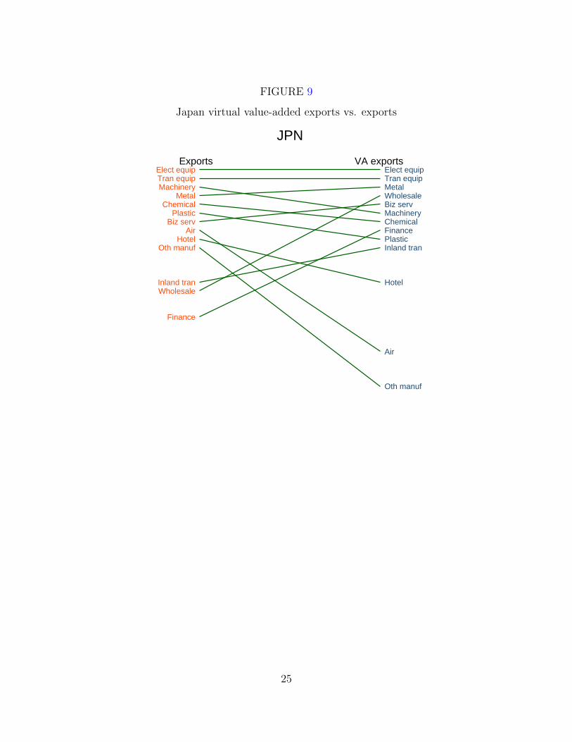
FIGURE 9

Japan virtual value-added exports vs. exports

ChemicalPlastic

MetalMachinery

Elect equipTran equip

Oth manuf

Wholesale

Hotel

Inland tran

Air

Finance

Biz serv Chemical

Plastic

Metal

Machinery

Elect equipTran equip

Oth manuf

Wholesale

Hotel

Inland tran

Air

Finance

Biz serv

Exports VA exports

JPN

25

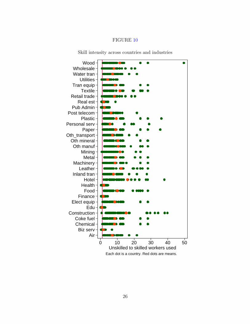
FIGURE 10

Skill intensity across countries and industries

AirBiz serv

ChemicalCoke fuel

ConstructionEdu

Elect equipFinance

FoodHealthHotel

Inland tranLeather

MachineryMetal

MiningOth manuf

Oth mineralOth_transport

PaperPersonal serv

PlasticPost telecom

Pub AdminReal est

Retail tradeTextile

Tran equipUtilities

Water tranWholesale

Wood

0 10 20 30 40 50Unskilled to skilled workers used

Each dot is a country. Red dots are means.

26

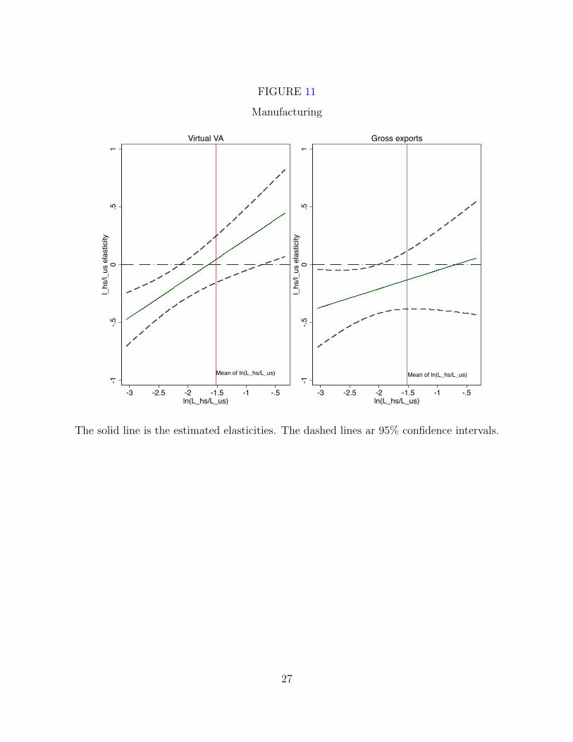
FIGURE 11

Manufacturing

Mean of ln(L_hs/L_us)

-1-.5

0.5

1l_

hs/l_

us e

last

icity

-3 -2.5 -2 -1.5 -1 -.5ln(L_hs/L_us)

Virtual VA


-1-.5

0.5

1l_

hs/l_

us e

last

icity

-3 -2.5 -2 -1.5 -1 -.5ln(L_hs/L_us)

Gross exports

The solid line is the estimated elasticities. The dashed lines ar 95% confidence intervals.

27

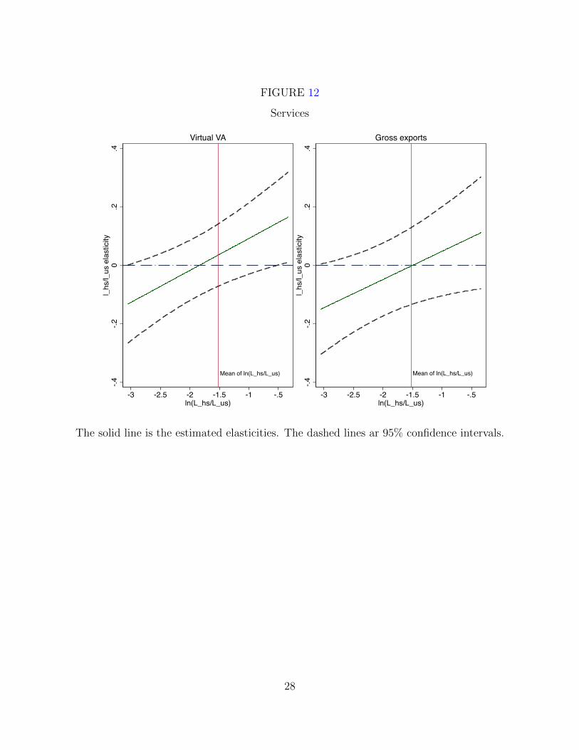
FIGURE 12

Services


-.4-.2

0.2

.4l_

hs/l_

us e

last

icity

-3 -2.5 -2 -1.5 -1 -.5ln(L_hs/L_us)

Virtual VA


-.4-.2

0.2

.4l_

hs/l_

us e

last

icity

-3 -2.5 -2 -1.5 -1 -.5ln(L_hs/L_us)

Gross exports

The solid line is the estimated elasticities. The dashed lines ar 95% confidence intervals.

28

heckscher-ohlin: evidence from virtual trade in value added · 2015-08-12 · heckscher-ohlin:...

Documents