heat pipe temperature control utilizing a soluble gas ... · heat pipe temperature control...
TRANSCRIPT

tx
I
oI
Heat Pipe Temperature Control UtilizingA Soluble Gas Absorption Reservoir
NASA CR-137,792
February 1976
by E. W. Saaski
Manager, Therma l Sys tems
Sigma Research , Inc.
2952 George Washington Way
Richland, Washington 99351
Prepared for
Ames Research Center
Nat ional Aeronaut ics and Space Administrat ion
Moffet Field. Cal i forn ia 94035
LM163767E
33.1380
https://ntrs.nasa.gov/search.jsp?R=19760013333 2018-09-03T10:47:56+00:00Z
This document is the final report submitted bySigma Research, Inc., Richland, Washington, for theprogram entitled "Heat Pipe Temperature ControlUtilizing a Soluble Gas Absorption Reservoir"(NASA Order No. A 13415B). C. McCreight andM. Groll were the NASA Technical Managers.
This report covers the period 12 May 1975 through7 November 1975.
NASA CR 137,79,2
HEAT PIPE TEMPERATURE CONTROL UTILIZING
A SOLUBLE GAS ABSORPTION RESERVOIR
by
E. W. Saaski
February 1976
Distribution of this report is provided in theinterest of information exchange. Responsibilityfor the contents resides in the author ororganization that prepared it.
Sigma Research, Inc.2952 George Washington WayRichland, Washington 99352
for
AMES RESEARCH CENTERNATIONAL AERONAUTICS AND SPACE ADMINISTRATION
MOFFETT FIELD, CALIFORNIA 94035

ABSTRACT
A new gas-controlled heat pipe design isdescribed which uses a liquid matrix reservoir,or sponge, to replace the standard gas reservoir.Reservoir volume may be reduced by a factor offive to ten for certain gas-liquid combinations,while retaining the same level of temperaturecontrol. Experiments with ammonia, butane, andcarbon dioxide control gases with methanolworking fluid are discussed.
CONTENTS
Page
SYMBOL TABLE ii
FIGURES 1v
TABLES X' v
1.0 INTRODUCTION 1
2.0 ANALYSIS 2
2.1 Basic Operating Theory 2
2.2 Candidate Gas/Fluid Systems 6
2.3 Transient Response-Reservoir Design 17
2.3.1 Reservoir Response-Slab Model 18
2.3.2 Coupled Heat Transfer-Diffusion Problem 26
2.3.2.1 Conservation of Noncondensable Gas 26
2.3.2.2 Conservation of Energy 27
2.3.2.3 Numerical Methods 28
2.4 Analytical Summary 30
3.0 EXPERIMENTAL VERIFICATION 31
3.1 Experimental Methods and Apparatus 31
3.1.1 Experimental Design 31
3.1.2 Testing Methods 35
3.2 Experimental Results 36
3.3 Data Interpretation . 36
3.3.1 Temperature Control 36
3.3.2 Transient Response 43
4.0 CONCLUSIONS 47
REFERENCES 49
APPENDIX A A-l
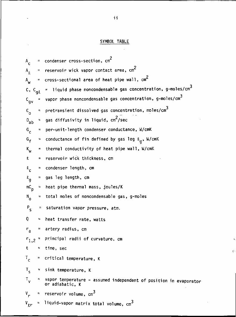
SYMBOL TABLE
2A = condenser cross-section, cm
2A = reservoir wick vapor contact area, cm
2A = cross-sectional area of heat pipe wall, cmW
3C, C . = liquid phase noncondensable gas concentration, g-moles/cm
3C = vapor phase noncondensable gas concentration, g-moles/cm
C = pretransient dissolved gas concentration, moles/cm.._
D . = gas diffusivity in liquid, cm /sec
G = per-unit-length condenser conductance, W/cmK
G^ = conductance of fin defined by gas leg I , W/cmK
K = thermal conductivity of heat pipe wall, W/cmK
i = reservoir wick thickness, cm
I - condenser length, cm
H = gas leg length, cm
mC = heat pipe thermal mass, joules/K
NQ = total moles of noncondensable gas, g-moles
PS = saturation vapor pressure, atm.
Q = heat transfer rate, watts
r = artery radius, cmd
rl 2 ~ Principal radii of curvature, cm
t = time, sec
TC = critical temperature, K
TS = sink temperature, K
T = vapor temperature - assumed independent of position in evaporatoror adiabatic, K
V = reservoir volume, cm3
= liquid-vapor matrix total volume, cm3
a = Ostwald coefficient
3 = fraction of condenser filled with wick/fluid compositeL*
6 = fraction of reservoir filled with wick/fluid composite
Y = surface tension, dynes/cm
5 = gap width, cm
n = fraction of wick/fluid composite filled with fluid in condenserL.
nr = fraction of wick/fluid composite filled with fluid in reservoir
6 = See equation 6L*
Qr = See equation 6
6+ = See equation 19
TQ = diffusive time constant, secTth = thermal time constant, sec
<C> = average value of C
IV
FIGURES
Page
2.1 A Comparison of Gas Reservoir and Gas Absorption Reservoir 3Heat Pipe Condenser Assemblies
2.2 The Solubility of Chlorine in CC14 and R-ll (CFClg) 7
2.3 Solubility of Various Gases in Methanol as a Function of 11Temperature
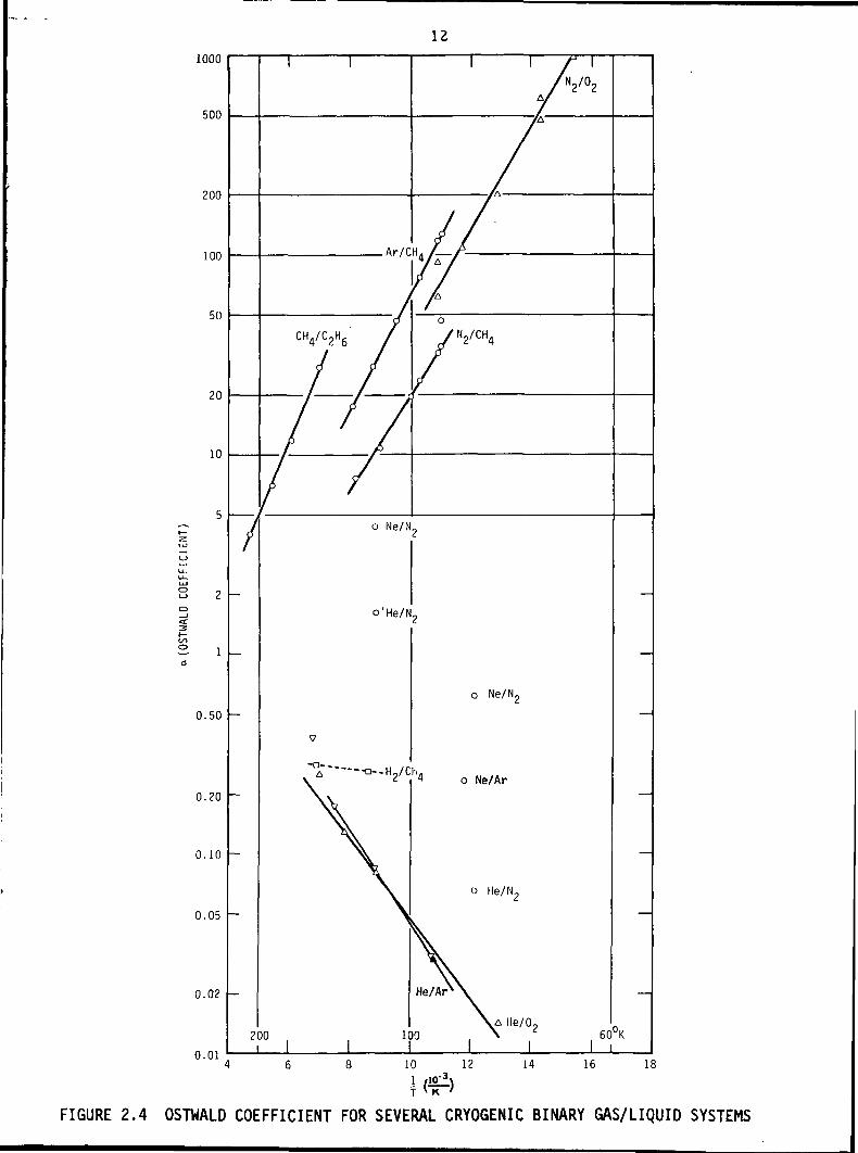
2.4 Ostwald Coefficient for Several Cryogenic Binary Gas/ 12Liquid Systems
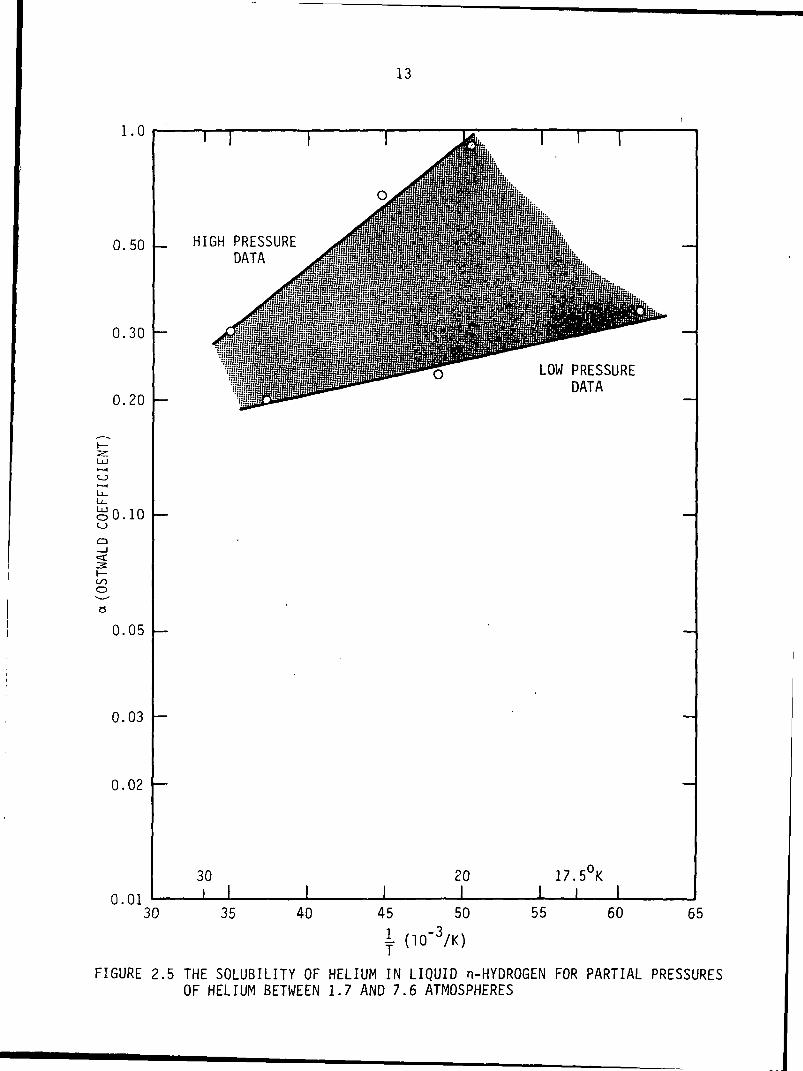
2.5 The Solubility of Helium in Liquid n-Hydrogen for 13Partial Pressures of Helium Between 1.7 and 7.6 Atmospheres
2.6 One-Dimensional Slab Model of Absorption Reservoir Unit Cell 19
2.7 Dimensionless Average Concentration in a Slab as a Function 20of the Grouping D . t/fi.2.
2.8 A Comparison of the Data of Ricci with the WiIke-Chang 22Empirical Model for Gas/Liquid Diffusivity
2.9 Predicted Diffusivities for Various Gas-Liquid Combinations 24That are of Interest for Gas-Absorption Reservoirs atCryogenic Temperatures
3.1 Details of Absorption Reservoir Design 33
3.2 Temperature Difference Between Heat Pipe Vapor Core and 37Condenser Heat Sink for the Control Gases n-C.H,Q and CCL
3.3 Temperature Difference Between Heat Pipe Vapor Core and 38Condenser Heat Sink for Ammonia Control Gas
3.4 Temperature Difference Between Heat Pipe Vapor Core and 39Condenser Heat Sink for Nitrogen Control Gas
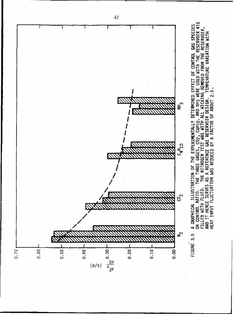
3.5 A Graphical Illustration of the Experimentally Determined 42Effect of Control Gas Species on Set-Point Stability
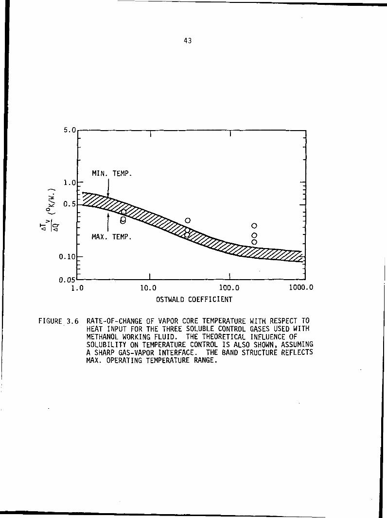
3.6 Rate of Change of Vapor Core Temperature with Respect to 43Heat Input for the Three Soluble Control Gases Used withMethanol Working Fluid
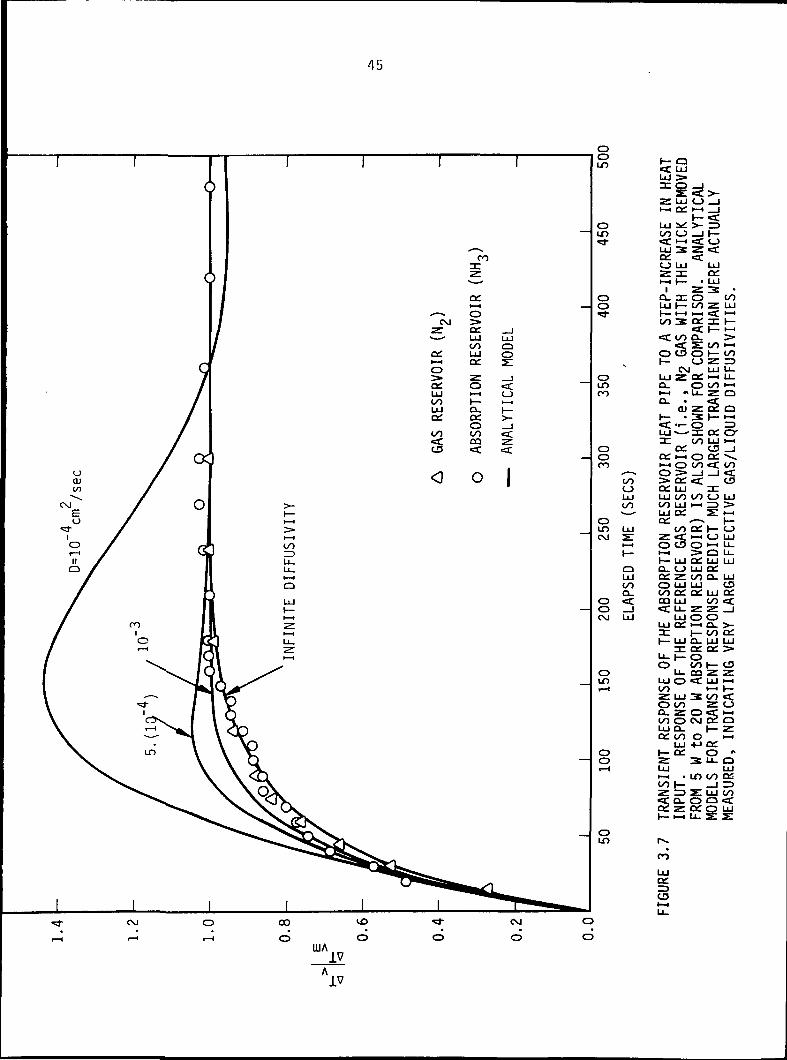
3.7 Transient Response of the Absorption Reservoir Heat Pipe to 45a Step-Increase in Heat Input

TABLES
Page
2.1 Experimental Ostwald Coefficients at 25°C for a 8Number of Gases and Fluids
2.2 Room Temperature Gas-Liquid Combinations Having High 10Solubility
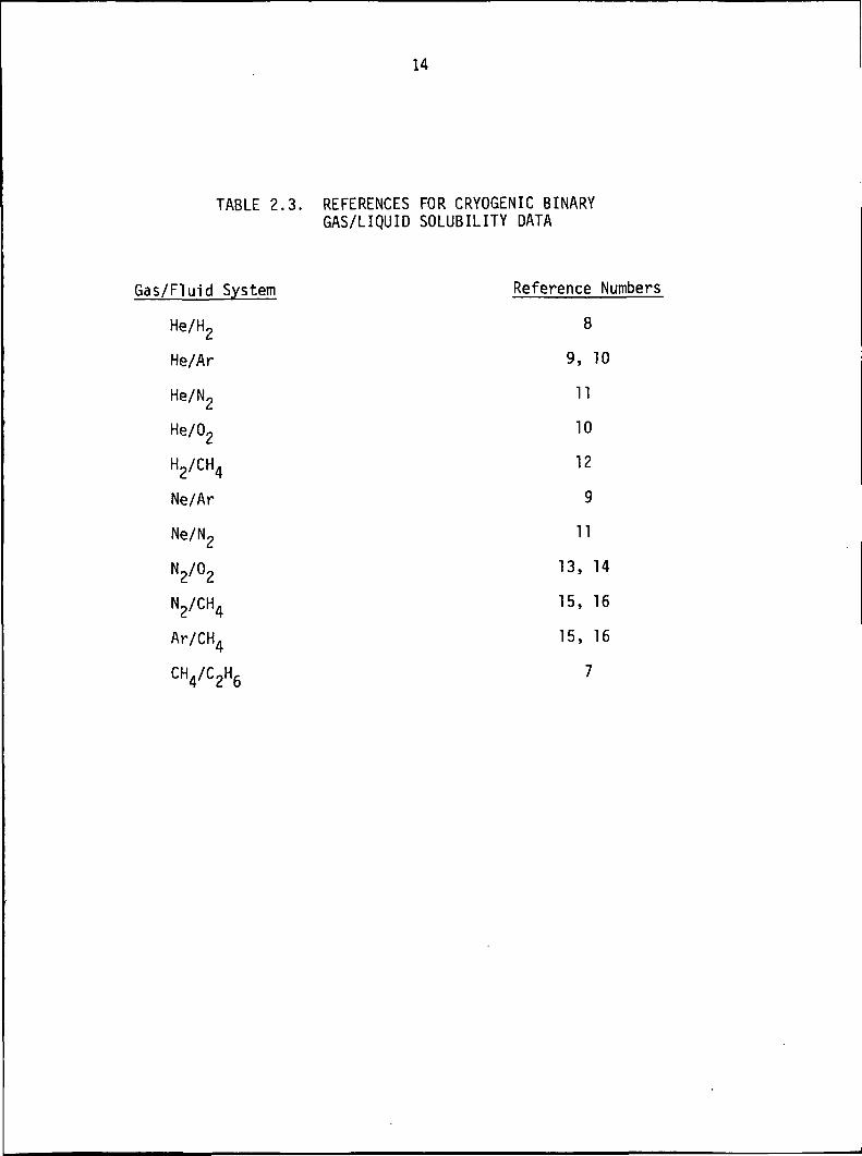
2.3 References for Cryogenic Binary Gas/Liquid Solubility Data 14
2.4 Curve-Fitting Constants for Binary Cryogenic Systems 16Showing Exponential Solubility Behavior
2.5 Diffusion Time Constants for Various Cryogenic Gas/ 25Liquid Binary Systems
3.1 Reservoir Specifications/Conductance Parameters . 34
3.2 Experimental Data Summary for Various Gas Control Tests 40With Methanol Working Fluid and a Reservoir Temperatureof 11 to 13°C
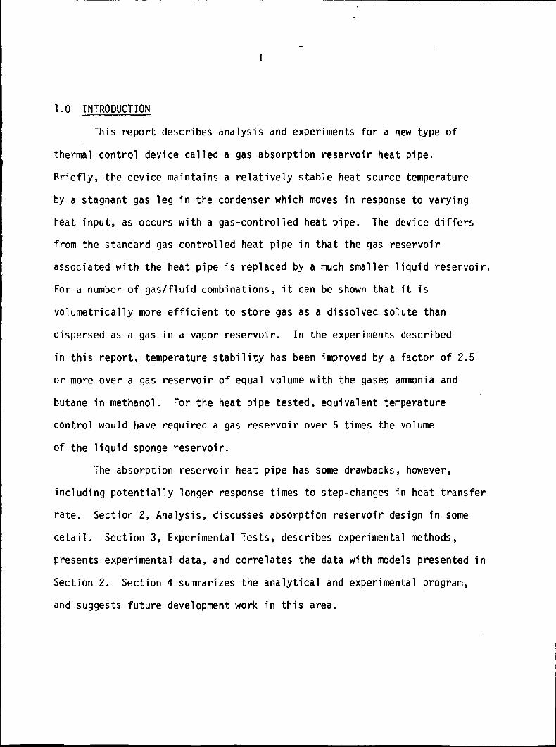
1.0 INTRODUCTION
This report describes analysis and experiments for a new type of
thermal control device called a gas absorption reservoir heat pipe.
Briefly, the device maintains a relatively stable heat source temperature
by a stagnant gas leg in the condenser which moves in response to varying
heat input, as occurs with a gas-controlled heat pipe. The device differs
from the standard gas controlled heat pipe in that the gas reservoir
associated with the heat pipe is replaced by a much smaller liquid reservoir.
For a number of gas/fluid combinations, it can be shown that it is
volumetrically more efficient to store gas as a dissolved solute than
dispersed as a gas in a vapor reservoir. In the experiments described
in this report, temperature stability has been improved by a factor of 2.5
or more over a gas reservoir of equal volume with the gases ammonia and
butane in methanol. For the heat pipe tested, equivalent temperature
control would have required a gas reservoir over 5 times the volume
of the liquid sponge reservoir.
The absorption reservoir heat pipe has some drawbacks, however,
including potentially longer response times to step-changes in heat transfer
rate. Section 2, Analysis, discusses absorption reservoir design in some
detail. Section 3, Experimental Tests, describes experimental methods,
presents experimental data, and correlates the data with models presented in
Section 2. Section 4 summarizes the analytical and experimental program,
and suggests future development work in this area.

2.0 ANALYSIS
The first section presents basic equations describing the steady-state
response of a gas-absorption reservoir heat pipe and compares the derived
equations with those for a gas-controlled heat pipe embodying a gas reservoir.
The next section discusses possible gas-liquid combinations for room-temperature
and cryogenic operation found from a literature search. The third and last
section addresses the effect of rapid source strength variations, which may
temporarily drive the gas absorption reservoir heat pipe to higher than
equilibrium operating temperatures because of a rate-limiting process of gas
diffusion into the liquid reservoir.
2.1 Basic Operating Theory
Figure 2.1 presents a comparison between the standard gas-controlled
heat pipe and the gas absorption reservoir heat pipe. The standard design
comprises a condenser active length a and a gas reservoir of volume Vr.
The equivalent gas absorption reservoir heat pipe has a liquid storage volume
storing V?R volume of fluid and gas, but is otherwise identical to the first
heat pipe. Each has a total cross-sectional area A in the condenser, which
is independent of axial position.
If for purposes of comparison the gas front is assumed sharp (i.e., a
flat front), then simple closed-form models of the two systems are possible.
For thermal comparison, assume it is necessary to design a gas-controlled heat
pipe with the following constraints:
1. At vapor core temperature T,, the gas front shall be at I = I .
2. At vapor core temperature T2, the gas front shall be at I = 0.
3. The sink temperature is T_, and the gas zone can be assumed
to also be at T.
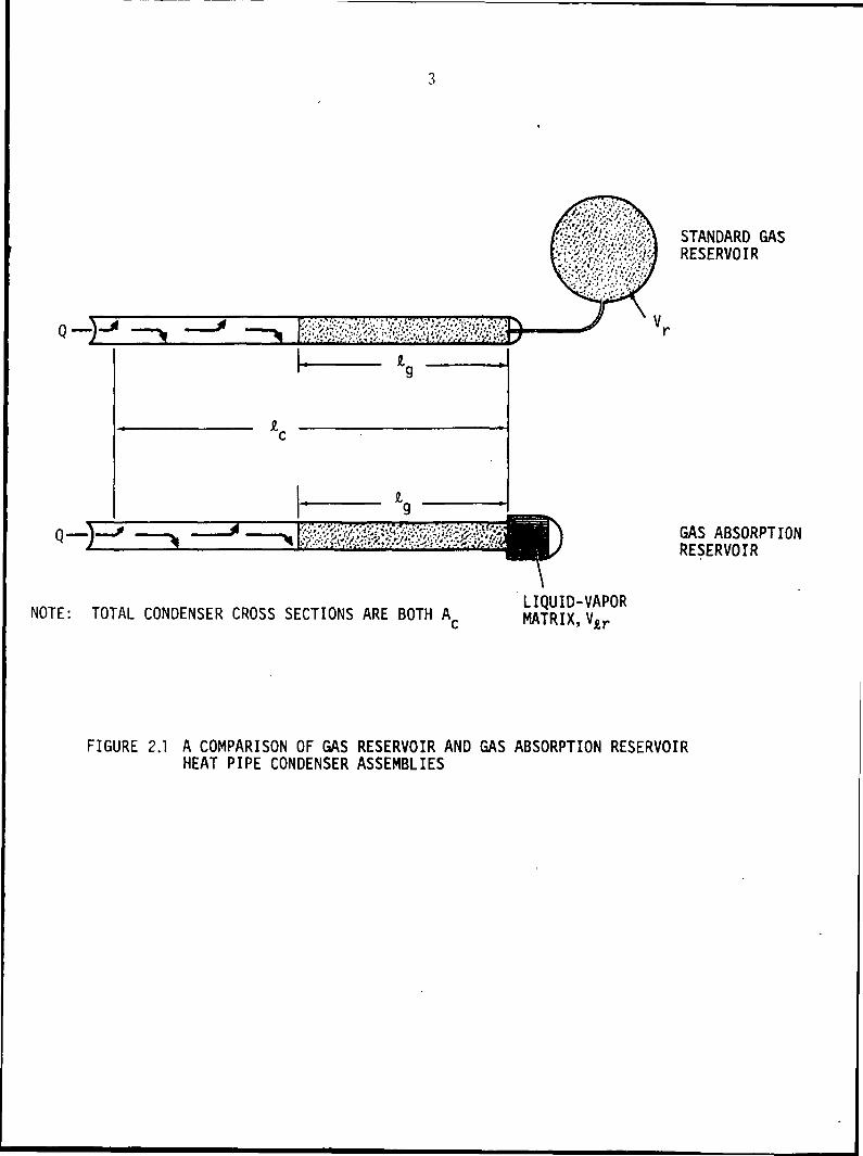
STANDARD GASRESERVOIR
NOTE: TOTAL CONDENSER CROSS SECTIONS ARE BOTH ALIQUID-VAPORMATRIX,V£r
GAS ABSORPTIONRESERVOIR
FIGURE 2.1 A COMPARISON OF GAS RESERVOIR AND GAS ABSORPTION RESERVOIRHEAT PIPE CONDENSER ASSEMBLIES
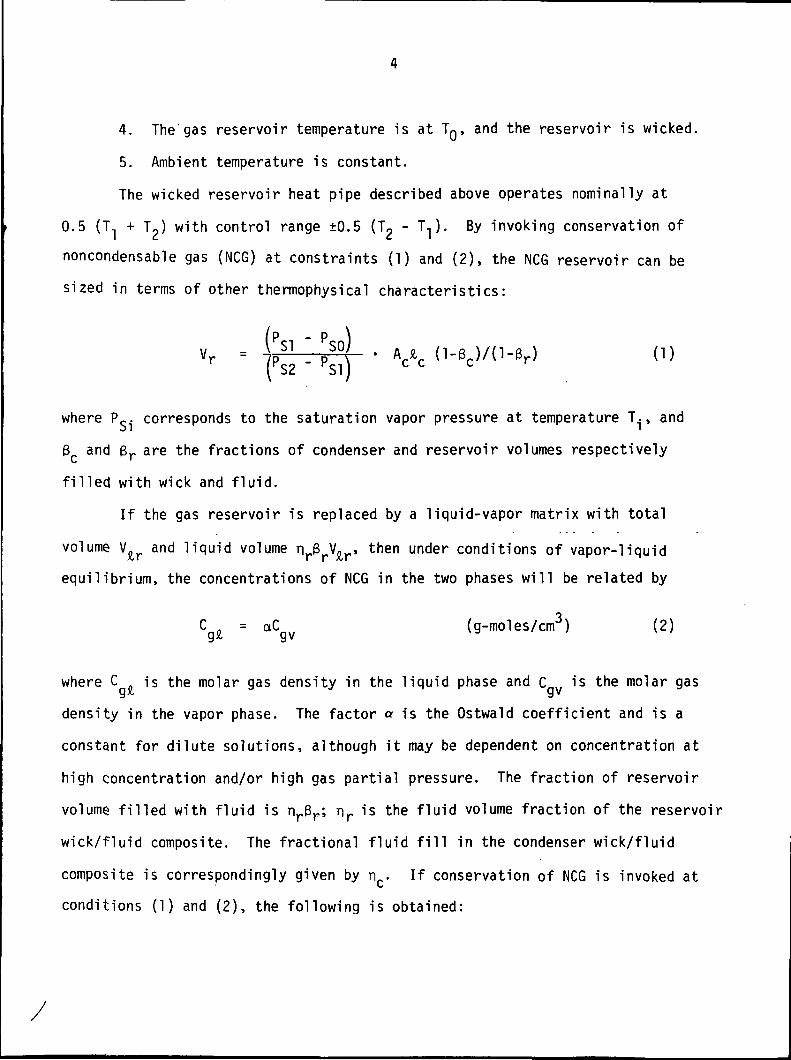
4. The gas reservoir temperature is at TQ, and the reservoir is wicked.
5. Ambient temperature is constant.
The wicked reservoir heat pipe described above operates nominally at
0.5 (TI + T2) with control range ±0.5 (T2 - T.J). By invoking conservation of
noncondensable gas (NCG) at constraints (1) and (2), the NC6 reservoir can be
sized in terms of other thermophysical characteristics:
*e*c «-Bc>/0-er) (1)
where P^. corresponds to the saturation vapor pressure at temperature T., and
3 and 6r are the fractions of condenser and reservoir volumes respectively
filled with wick and fluid.
If the gas reservoir is replaced by a liquid-vapor matrix with total
volume V£r and liquid volume n V , then under conditions of vapor-liquid
equilibrium, the concentrations of NCG in the two phases will be related by
C £ = aCgv (g-moles/cm3) (2)
where C is the molar gas density in the liquid phase and C is the molar gas
density in the vapor phase. The factor a is the Ostwald coefficient and is a
constant for dilute solutions, although it may be dependent on concentration at
high concentration and/or high gas partial pressure. The fraction of reservoir
volume filled with fluid is nr8r; nr is the fluid volume fraction of the reservoir
wick/fluid composite. The fractional fluid fill in the condenser wick/fluid
composite is correspondingly given by n . If conservation of NCG is invoked atC
conditions (1) and (2), the following is obtained:

where
No = Cgv (T l } AA9c + W (Condition ^
NQ = Cgv(T2)9 rVAr (Condition 2) (4)
P - PSi SO (5)v 'RTQ
and
ec = i + Bc(anc-D; er = 1 + Br(<xnr-D (6)
If expressions (3) and (4) are set equal to each other and V^r is solved for,
it is found that
.. (pS2-psl) c r
If, for purposes of comparison, it is assumed in equation (7) that n is
very close to 1.0 and 3 is much less than 1.0, then it is clear that expres-
sions (1) and (7) differ by only the multiplicative constant l/cx3 if 8 and
3r are both small in equation (1) and a is much larger than one. That is,
the required liquid reservoir volume for a given amount of temperature control
is on the order of l/a8 times the gaseous volume needed in a typical gas
reservoir heat pipe.
Phrased another way, if gas/fluid combinations can be found where a is
significantly greater than 1.0 and n 3 is small, then it is volumetricallyc c
more efficient to store the gas as a dissolved solute than dispersed in a vapor
phase reservoir. Such combinations are possible but common control gases do
not satisfy this criteria.

2.2 Candidate Gas/Fluid Systems
As discussed in Section 2.1, it is volumetrically more efficient to store
a noncondensable gas in the form of a dissolved solute than to store the gas
dispersed in a vapor phase if the Ostwald coefficient is greater than 1. It is
thus desirable to use systems with the highest Ostwald coefficient possible for
gas absorption heat pipes, unless very high solubility contributes to deleterious
side effects.
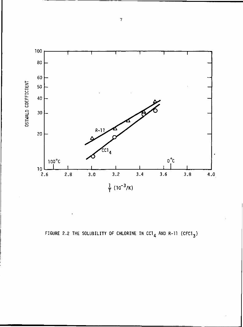
Stable heat pipe operation has been previously demonstrated for a in
the range 20 to 30. In Reference 1, Saaski operated both C12/CC14 and C12/CFC13
systems in the reflux mode for temperatures between 10° and 100°C with satisfactory
component separation. Ostwald coefficients as a function of temperature are
shown in Figure 2.2. Both carbon tetrachloride and R-ll are unfortunately
rather poor heat pipe fluids, and a literature search was accomplished to
determine if there existed more optimum fluid/gas combinations.
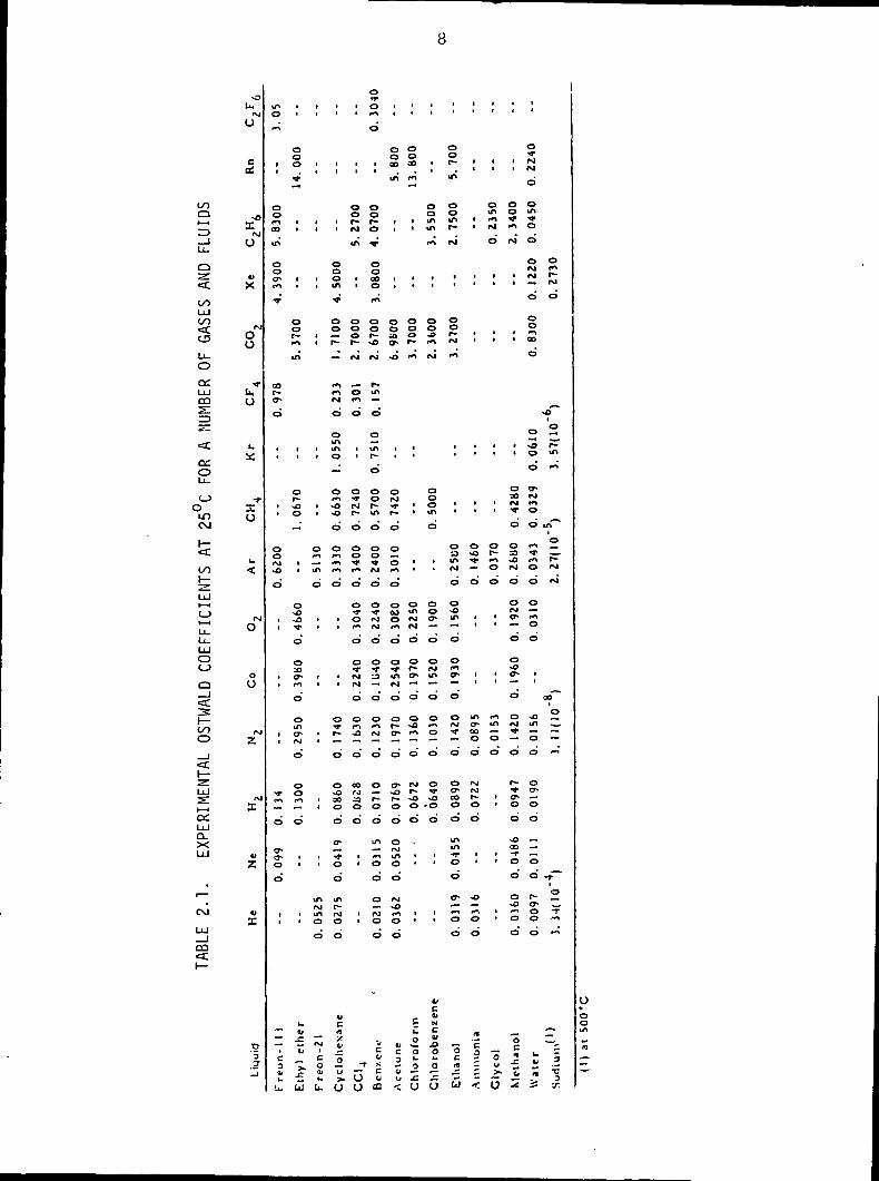
Table 2.1 presents Ostwald coefficient data from Reference 2 for a large
number of gas/liquid combinations at 25°C. The common control gases such as He,
Np and Ar are seen to have Ostwald coefficients strictly less than 1, and are
unsatisfactory. Large molecules such as Kr, CO^, Xe and C2Hg do have Ostwald
coefficients greater than 1, but the largest value is on the order of 5. This
is somewhat marginal. To demonstrate a significant advantage over present gas
reservoir designs, it would be desirable to use a gas/fluid combination with
an Ostwald coefficient of 10 to 20. As discussed in Section 2.3, some void
volume must be left in the reservoir for optimum reservoir response, and a
fluid/wick volume fraction BR of 0.5 is a realistic goal. Reservoir size
reduction would therefore be on the order of 1/5 to 1/10.
LUI-H
o
oo
ooo
100
80
60
50
40
30
20
10
100°CI I
2.6 2.8
R-ll
0°C
3.0 3.2 3.4 3.6 3.8
(10"3/K)
4.0
FIGURE 2.2 THE SOLUBILITY OF CHLORINE IN CC14 AND R-ll (CFC13)
8
ooo
oo<oU_
O
OLLUCOs:ZD—<ccz.o
oIDC\J
oo
Q
—I•a:
ooo
Q.X
CO
u°IM
u
OS
-OX
<j"
t>X
IMOo
•Vfu,u
I.X
"fXo
u<
IM
o
ou
fM2
IMX
4)z
41X
0'3.j
inO
»-i
i
oo1-100
in
o0o»r-»
•r
COr-crd
,i
•
ooIM•O
d
i
f•
i
r»-i
d
9*O
d
i
-~
Fre
on
- 1 1
,
o0o•f
,
t
oo1—min
,|
or-»oo
—
1
o*o•a*rd
o30CT-fl
d
oina*rM
o'
oor->
d
1
|
h*Of.c41
>.-C
U
i i
i i
i >i i
oo
I Oi in
1-
oo
1 — «1 1—
—l*%f"tIM
d
oin
i in• O
-om
1 -Oi 0
d
o o<»i m—t *v*l
in m
d d
i i• '
i i' '
o*r
• r-
d
o0i 001 O
d
a*i *f• od
m mIM r-in IM0 0
d d
41crt
Fre
on
-21
Cyclo
lle
x
0*r
i O
d
i ii i
o o0 0r- r-IM 0
in V
o0
• 00• o
r*%
O O0 0o r*r- -aIM rM
— r-o inr —•d d
oi ini r-d
o o•* oIM r-r- m
d d
o oo o•f Tf> IM
d d
o o••r TO IMr*< PJ
O O
O OT *rfM 13IM — •
0 0
O Of* **S«O IM
d d
00 Or>) -*a r-o od d
in
i <^i< od
oi fMi O
d
CC
14
Bcn
/.e
nc
i i
0 00 0CO 00
in f>
i •i i
i >* i
0 00 0iO 0o- i-,0 f«
1 «• '
0rM•+ 'r- •
d
0o 'r*\ 'd
o ooj m0 <M1-1 IM
0 0
0 0•«• f~m wfM -*
o o
o or *oo *•"»
0 0
(7- «M-o r-r- ~00 0
d d
orMin i0 •d
fM•o1 1 io •d
£u
Ac
eto
ne
Ch
loro
fo
i
i
ooinmm
;
oo*di*>
fM
OOoino"
;
o0V-*o
ofMin~"a
oo
o
oro.0
d
i•
;
ucOfNC
Ch
loro
be
'
oor-in
00inr-fM~
f
00r*fM
t*\
i*
I
o33infM
d
ooin"™0
o(•o»^
o
ofMT
O
0o*CO0
d
min*rod
<r-
od
Eth
an
ol
i
i
ti
i
'
•
'
1
0NO
•f
d
•1
i1
mo*000
o
fM<Mf-O
d
i•
sO
f*od
in
Am
mo
ni;
'
i
0m**>fM
d
!
i
11
•
of-f»>od
1
*
i'
i*inoo
:
t1
t
"ou>-5
i• i
0"
I fM> IM
d
0 0o «n•* Tm 0
rj 0
0 0fM 1*
• IM r~i — . IM
d d
oo
i 00
d
_•ooo _
I *0 f~-t o *^*
d f>
O <T-00 IMfM **T O
d d ,n"~"o0 f« _
=0 •»>O ro <*•fM O <M
d d IM
O O
fM —fj* i-• O
d d
o*oO^ 1
~" 'd oo~
oo -o _IM m -_-TJ. _ __ o —O O f^
r- o* C"
<7- —O O
d d
•o —CO —•r •—o od d ~~
oo r- _*O C7 »*s O TO O ~i
d d ••>
^ ••" «"O C;_
1 t 3
i 3 1*i ^ -S.
0•ooin
n>
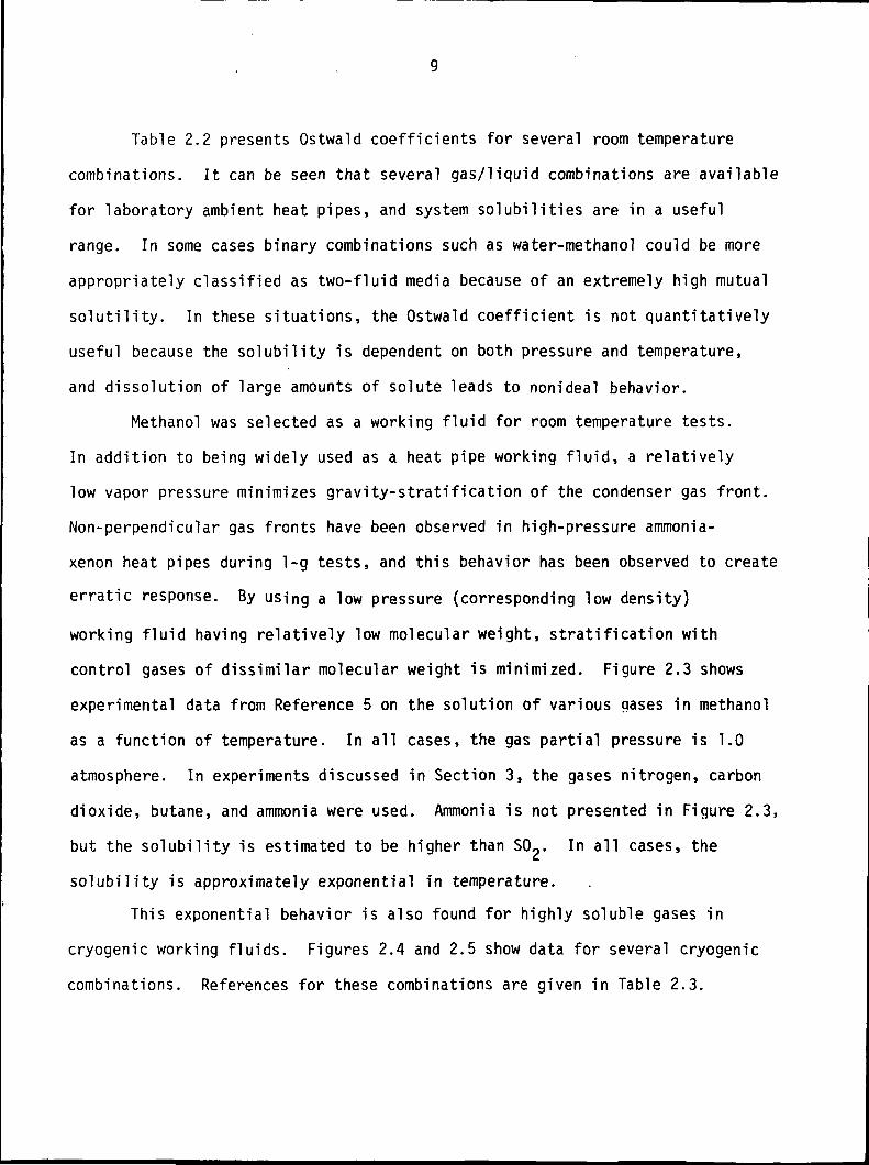
Table 2.2 presents Ostwald coefficients for several room temperature
combinations. It can be seen that several gas/liquid combinations are available
for laboratory ambient heat pipes, and system solubilities are in a useful
range. In some cases binary combinations such as water-methanol could be more
appropriately classified as two-fluid media because of an extremely high mutual
solutility. In these situations, the Ostwald coefficient is not quantitatively
useful because the solubility is dependent on both pressure and temperature,
and dissolution of large amounts of solute leads to nonideal behavior.
Methanol was selected as a working fluid for room temperature tests.
In addition to being widely used as a heat pipe working fluid, a relatively
low vapor pressure minimizes gravity-stratification of the condenser gas front.
Non-perpendicular gas fronts have been observed in high-pressure ammonia-
xenon heat pipes during 1-g tests, and this behavior has been observed to create
erratic response. By using a low pressure (corresponding low density)
working fluid having relatively low molecular weight, stratification with
control gases of dissimilar molecular weight is minimized. Figure 2.3 shows
experimental data from Reference 5 on the solution of various gases in methanol
as a function of temperature. In all cases, the gas partial pressure is 1.0
atmosphere. In experiments discussed in Section 3, the gases nitrogen, carbon
dioxide, butane, and ammonia were used. Ammonia is not presented in Figure 2.3,
but the solubility is estimated to be higher than SO^. In all cases, the
solubility is approximately exponential in temperature.
This exponential behavior is also found for highly soluble gases in
cryogenic working fluids. Figures 2.4 and 2.5 show data for several cryogenic
combinations. References for these combinations are given in Table 2.3.

10
TABLE 2.2 ROOM TEMPERATURE GAS-LIQUID COMBINATIONS HAVINGHIGH SOLUBILITY
Solvent
Hexane
Benzene
Benzene
Menthanol
Menthanol
Menthanol
Menthanol
Menthanol
Water
Water
Water
Solute
n-Propane
n-Propane
n-Pentane
Propane
Carbon Dioxide
Butane
Sulfur Dioxide
Carbon Dioxide
Ammonia
Sulfur Dioxide
Menthanol
Temperature(°0
25
25
16
25
12
12
25
59
25
25
100
OstwaldCoefficient
23.6
16.0
312.0
3.4
4.1
28.0
83.0
39.0
40.7
34.0
254.0
Ref
(3)
(3)
(4)
(5)
(5)
(5)
(5)
(6)
(5)
(5)
(7)

11
10-1
oCO
10-3
10-4
25°C 100°C
Q ESTIMATED
i I
2.3 2.72.5LOG1Q(T) (T IN K)
FIGURE 2.3 SOLUBILITY OF VARIOUS GASES IN METHANOL AS A FUNCTION OFTEMPERATURE (FROM REFERENCE 5)
12
1000
500
o(_>o
0.50 -
0.20 ~
0.10 -
0.05 -
0.02 -
0.0118
FIGURE 2.4 OSTWALD COEFFICIENT FOR SEVERAL CRYOGENIC BINARY GAS/LIQUID SYSTEMS
13
1.0
0.50
0.30
0.20
. 10
o_ I•=c
COo
0.05
0.03
0.02
0.0130
HIGH PRESSUREDATA
30
35 40
20
45 50
(10~3/K)
LOW PRESSUREDATA
17.5°K
55 60 65
FIGURE 2.5 THE SOLUBILITY OF HELIUM IN LIQUID n-HYDROGEN FOR PARTIAL PRESSURESOF HELIUM BETWEEN 1.7 AND 7.6 ATMOSPHERES
14
TABLE 2.3. REFERENCES FOR CRYOGENIC BINARYGAS/LIQUID SOLUBILITY DATA
Gas/Fluid System Reference Numbers
He/H2 8
He/Ar 9, 10
He/N2 11
He/02 10
H2/CH4 12
Ne/Ar 9
Ne/N2 11
N2/02 13, 14
N2/CH4 15, 16
Ar/CH4 15, 16
CH4/C2H6 7

15
Table 2.4 gives fitting constants A and B for cryogenic combinations
of interest where the Ostwald coefficient is modeled as
« a A EXP(+B/T) (8)
and where T is the system temperature in degrees Kelvin. The exponential
coefficient B ranges from 550 to 1850 K and the pre-exponential factor is
between 0.07 and 0.10. Systems of potential interest include
1. methane/ethane
2. argon/methane
3. nitrogen/methane
4. nitrogen/oxygen
The solubility of helium in hydrogen is surprisingly low as shown in Figure 2.5
and, hence, this technique would not be practical for liquid hydrogen nor, of
course, helium.
The general exponential dependence of solubility on temperature is of
both beneficial and adverse effect. Because of the rapid solubility decrease
with temperature, condensate originating near the cold gas front becomes
supersaturated as the fluid warms in transit to the evaporator, and gas stripping
is augmented. This serves to maintain a sharp gas front. Conversely, the
sensitivity to temperature can create problems in set-point maintenance. If
liquid reservoir temperature is not maintained constant, the amount of dissolved
gas in the liquid will fluctuate in response to temperature variations. The
most direct consequence of this will be a fluctuation in both gas front position
and heat pipe operating temperature. This sensitivity to reservoir temperature
is also found in the wicked reservoir heat pipe where the reservoir working
fluid partial pressure is exponentially dependent on reservoir temperature.

16
TABLE 2.4. CURVE-FITTING CONSTANTS FOR BINARY CRYOGENICSYSTEMS SHOWING EXPONENTIAL SOLUBILITY BEHAVIOR
Gas/Liquid System A B (K)
CH,./C9HC 0.0713 848*\ f. b
Ar/CH4 0.0748 673
N2/CH4 0.0821 549
N2/02 0.100 599
17
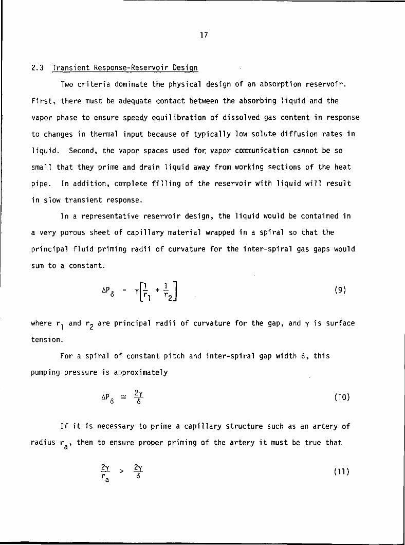
2.3 Transient Response-Reservoir Design
Two criteria dominate the physical design of an absorption reservoir.
First, there must be adequate contact between the absorbing liquid and the
vapor phase to ensure speedy equilibration of dissolved gas content in response
to changes in thermal input because of typically low solute diffusion rates in
liquid. Second, the vapor spaces used for vapor communication cannot be so
small that they prime and drain liquid away from working sections of the heat
pipe. In addition, complete filling of the reservoir with liquid will result
in slow transient response.
In a representative reservoir design, the liquid would be contained in
a very porous sheet of capillary material wrapped in a spiral so that the
principal fluid priming radii of curvature for the inter-spiral gas gaps would
sum to a constant.
*y (9)
where r, and r~ are principal radii of curvature for the gap, and y is surface
tension.
For a spiral of constant pitch and inter-spiral gap width <5, this
pumping pressure is approximately
AP6 * f (10)
If it is necessary to prime a capillary structure such as an artery of
radius r,, then to ensure proper priming of the artery it must be true thata
18
If the heat pipe is tested in 1-g then the effects of gravity must also be
included.
Equation 11 presents a criterion relating minimum size of reservoir gas
gaps to characteristic capillary pumping structure dimensions in the heat pipe.
To characterize maximum fluid absorber thickness, and thereby define the void/
volume ratio in the reservoir, it is necessary to establish reservoir response
to fluctuating heat inputs.
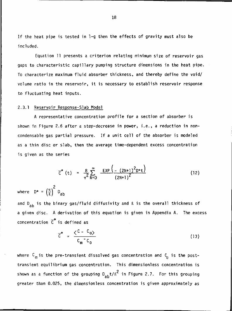
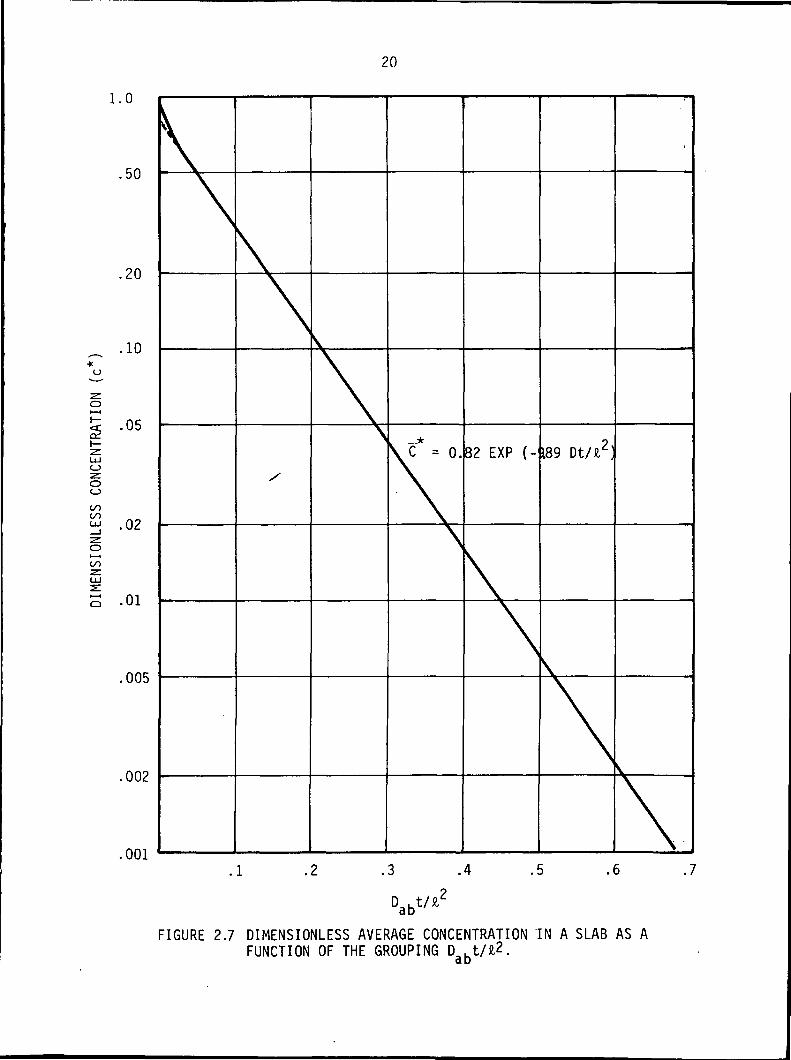
2.3.1 Reservoir Response-Slab Model
A representative concentration profile for a section of absorber is
shown in Figure 2.6 after a step-decrease in power, i.e., a reduction in non-
condensable gas partial pressure. If a unit cell of the absorber is modeled
as a thin disc or slab, then the average time-dependent excess concentration
is given as the series
C*(t) = «f EXP(- (2N+l)2D*t) (12)
TT N=0 (2N+1T
where D* = (£) Dab
and D , is the binary gas/fluid diffusivity and I is the overall thickness ofaoa given disc. A derivation of this equation is given in Appendix A. The excess
_*concentration C is defined as
-* <C- Co>(13)
c m" c o
where C m i s the pre-transient dissolved gas concentration and C is the post-
transient equilibrium gas concentration. This dimensionless concentration is2
shown as a function of the grouping D . t/£ in Figure 2.7. For this grouping
greater than 0.025, the dimensionless concentration is given approximately as

19
POROUSABSORBER
DISSOLVED GASCONCENTRATIONPROFILE
FIGURE 2.6 ONE-DIMENSIONAL SLAB MODEL OF ABSORPTION RESERVIOR UNITCELL. WITH A STEP-CHANGE IN EXTERNAL GAS CONCENTRATION,THE POROUS LIQUID-SATURATED ABSORBER RE-ESTABLISHESEQUILIBRIUM BY GAS/LIQUID DIFFUSION.
20
1.0
50
.20
.10
.05
ooo
"J .02o»—4CO
.01
.005
.002
.001.1
_*C = 0.82 EXP (- 189 Dt/i,2)
.2 .3 .4 .5 .6 .7
FIGURE 2.7 DIMENSIONLESS AVERAGE CONCENTRATION IN A SLAB AS AFUNCTION OF THE GROUPING Dabt/fc2.
21
C* as 0.82 EXP (-9.89 Dt/£2) (14)
At time equal zero, C" = 1 . , while at t = », c* = 0. At some finite
time C" is negligibly small. If C = 0.01 is arbitrarily selected as negligibly
small, then a characteristic time constant T for diffusion-driven equilibrium
is obtained
T = 0.446 *2/Dab (sees) (15)
Because cryogenic heat pipe design is currently of high interest and
fluid diffusivities can be expected to be low, values of T have been calculated
for several cryogenic fluids using the following expression for the diffusivity
9.76(10'8) (M.<
b a
whereo
Dab = diffusion coefficient, a+b (cm /sec)
M. = solvent molecular weight
<Jj = association parameter (water =2.6, methanol = 1.9, benzene = 1.0, etc.)
T = temperature (°K)
yb = solvent viscosity (centi poise)
a, = molecular diameter, A°d
This is a modified form of the Wi Ike-Chang empirical diffusivity formula
as given in Reference 2. Since this was derived from room temperature data, it
was necessary to check the model against experimental cryogenic data. This was
done for the data of Ricci (Ref. 17) for various gases in liquid nitrogen.
Figure 2.8 shows correlation of Ricci 's data with the empirical model (16) for
the gases Ne, Ar, and CH4- The temperature dependence of diffusivity is

22
100.
PI (REF.17)
(EQN.16)
} (NT3/*)
FIGURE 2.8 A COMPARISON OF THE DATA OF RICCI WITH THE WILKE-CHANGEMPIRICAL MODEL FOR GAS/LIQUID DIFFUSIVITY. LIQUIDNITROGEN IS SOLVENT.

23
represented very well, although the absolute values differ by as much as 30%.
However, this is adequate agreement for scoping purposes.
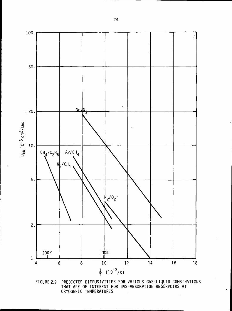
In the previous section, several cryogenic gas/liquid combinations were
identified as of potential interest. These were
1. methane/ethane
2. argon/methane
3. nitrogen/methane
4. nitrogen/oxygen
With the model (16), the diffusivities shown in Figure 2.9 were calculated.- 5 2 - 5 2The diffusivities are typically from 2 x 10 cm /sec to 10 x 10 cm /sec.
Before using these values of D . to calculate T, the values were multiplied by
0.40 to account for permeability of the porous slab used as a gas absorber.
This correction factor was based on the experimental data of Saaski (Ref. 2)
for double-thickness square-weave screens.
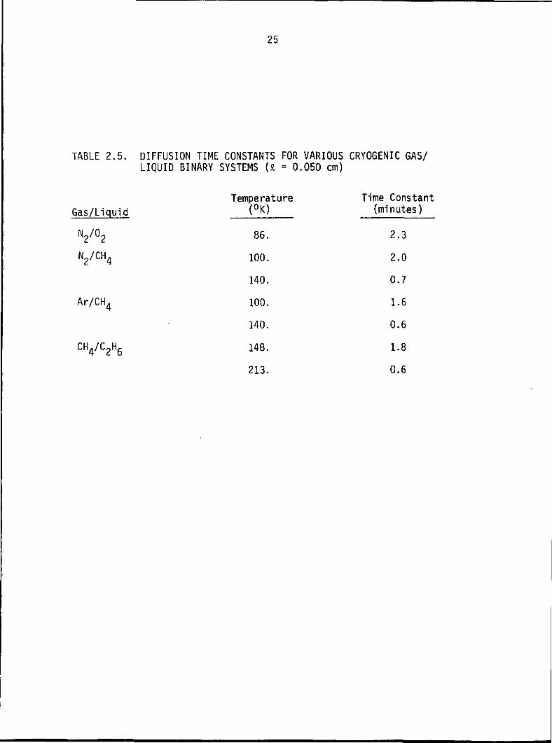
Characteristic time constants are presented in Table 2.5 for the fluids
previously noted, using Equation 16 and a correction factor of 0.40 to D . .
A slab thickness of 0.050 cm was selected as representative of absorber thickness:2
the time constant scales as £ for other thicknesses. For this particular
choice of £» time constants of 0.6 to 2.3 minutes are indicated. The time
constants are therefore not excessively long, but care must be exercised in
design so that the characteristic fluid films are of the order of 0.050 cm in
thickness. Even an increase to only 1.0 mm thickness results in time constants
of 2.4 and 9.2 minutes, respectively; the latter equilibration time could be
unsatisfactory in many thermal control systems.
24
100.
50.
. 20.
0)</>-••.Odeo
jQ03Q
10.
2.
CH/C2H6 Ar/CH
200 K
v
\ \
100K
10
(10"3/K)
12 14 16 18
FIGURE 2.9 PREDICTED DIFFUSIVITIES FOR VARIOUS GAS-LIQUID COMBINATIONSTHAT ARE OF INTEREST FOR GAS-ABSORPTION RESERVOIRS ATCRYOGENIC TEMPERATURES
25
TABLE 2.5. DIFFUSION TIME CONSTANTS FOR VARIOUS CRYOGENIC GAS/LIQUID BINARY SYSTEMS (A = 0.050 cm)
Temperature Time ConstantGas/Liquid (°K) (minutes)
Ar/CH4
CH4/C2H6
86.
100.
140.
100.
140.
148.
213.
2.3
2.0
0.7
1.6
0.6
1.8
0.6
26
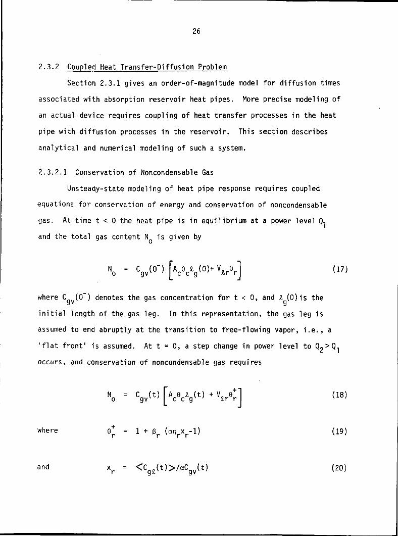
2.3.2 Coupled Heat Transfer-Diffusion Problem
Section 2.3.1 gives an order-of-magnitude model for diffusion times
associated with absorption reservoir heat pipes. More precise modeling of
an actual device requires coupling of heat transfer processes in the heat
pipe with diffusion processes in the reservoir. This section describes
analytical and numerical modeling of such a system.
2.3.2.1 Conservation of Noncondensable Gas
Unsteady-state modeling of heat pipe response requires coupled
equations for conservation of energy and conservation of noncondensable
gas. At time t < 0 the heat pipe is in equilibrium at a power level Q1and the total gas content N is given by
No
where C (0") denotes the gas concentration for t < 0, and £ (0)is the
initial length of the gas leg. In this representation, the gas leg is
assumed to end abruptly at the transition to free-flowing vapor, i.e., a
'flat front1 is assumed. At t = 0, a step change in power level to Qo>
occurs, and conservation of noncondensable gas requires
o = Cgv(t)
where Q+ = 1 + (^ (aryyl) (19)
= <Cg£(t)>/aCgv(t) (20)

27
It is assumed that diffusion of dissolved gas into and out of the
condenser wick is very rapid, and that the primary non-equilibrium condition
occurs in the reservoir fluid. Deviation from equilibrium conditions at
t > 0 is represented by x , which is the ratio of actual dissolved gas
concentration to the dissolved concentration at the vapor-liquid interface.
This interface is always assumed to be in equilibrium, that is,
C (t) = aC (t) (interface condition) (21)
The average dissolved gas concentration in the reservoir is
<C .(t)>. For a slab reservoir of thickness £, the average dissolved
concentration is expressed as
<CQ,(t)> = aC (0)+ ab /"* (dCg^ dt (22)gjt gv I I \ dx
This assumes that the slab is in vapor contact on both faces, as in Figure 2.6.
2.3.2.2 Conservation of Energy
At any instant in time, heat transferred to the heat pipe must be
accounted for by heat transfer through the condenser and/or by a temperature
increase of system thermal mass. For modeling ease, system thermal mass is
assumed always to be in equilibrium with the vapor core temperature, T (t).
Conservation of energy at t > 0 results in
* w (VTs' ,„.(23>
28
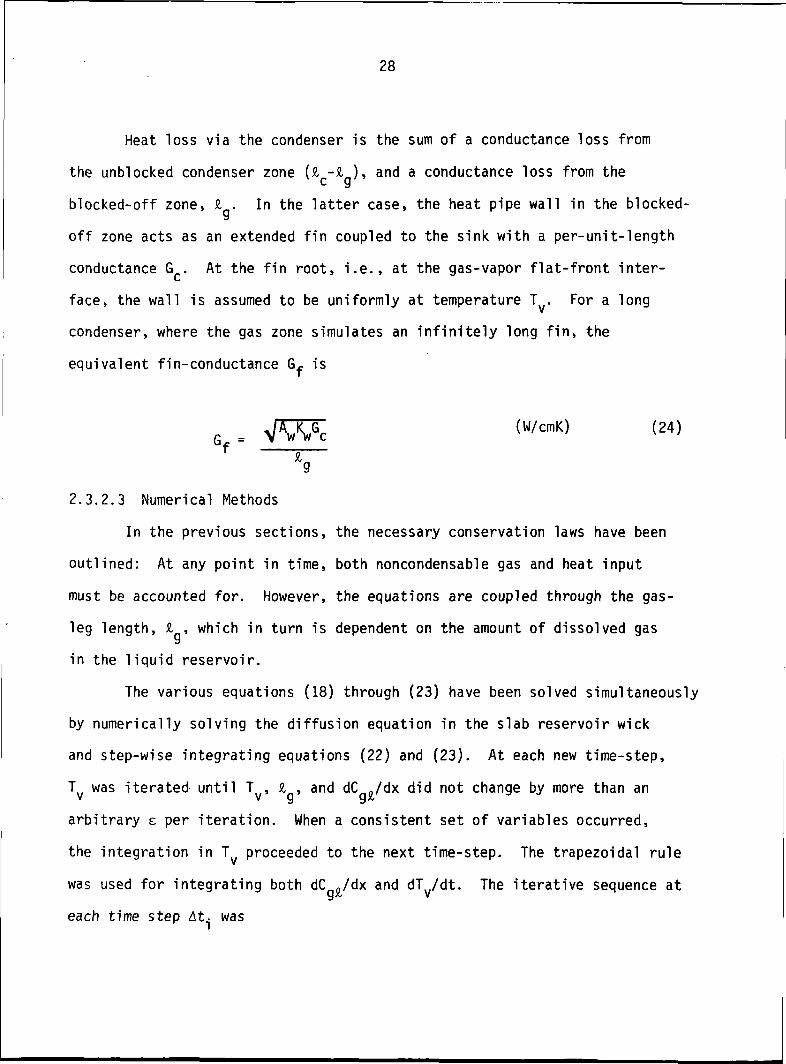
Heat loss via the condenser is the sum of a conductance loss from
the unblocked condenser zone (a -O> and a conductance loss from the
blocked-off zone, I . In the latter case, the heat pipe wall in the blocked-
off zone acts as an extended fin coupled to the sink with a per-unit-length
conductance G . At the fin root, i.e., at the gas-vapor flat-front inter-
face, the wall is assumed to be uniformly at temperature T . For a long
condenser, where the gas zone simulates an infinitely long fin, the
equivalent fin-conductance Gf is
(W/cmK) (24)
2.3.2.3 Numerical Methods
In the previous sections, the necessary conservation laws have been
outlined: At any point in time, both noncondensable gas and heat input
must be accounted for. However, the equations are coupled through the gas-
leg length, a , which in turn is dependent on the amount of dissolved gas
in the liquid reservoir.
The various equations (18) through (23) have been solved simultaneously
by numerically solving the diffusion equation in the slab reservoir wick
and step-wise integrating equations (22) and (23). At each new time-step,
T was iterated until T , £ , and dC ./dx did not change by more than an
arbitrary e per iteration. When a consistent set of variables occurred,
the integration in T proceeded to the next time-step. The trapezoidal rule
was used for integrating both dC 0/dx and dT.,/dt. The iterative sequence aty X» V
each time step At. was

29
1. Calculate T . from equation (23) using previous value of £ ;calculate C ..
2. Using C . and equation (21), calculate dC ./dxj usingfinite differences. x~
3. Calculate the average dissolved gas concentration using (22).
4. Determine 6+. from equations (19) and (20).
5. Determine a new £ . from equation (18).
6. Compare I . with i . of previous iteration. If A£ < e,continue to next time step. If A£ > e, go to step 1 and
yperform calculations using updated I ..
Representative unsteady-state solutions for the time-dependent vapor
core temperature T (t) are given in Figure 3.7. These solutions are based
on the experimental device detailed in Section 3.1, Experimental Methods
and Apparatus.
The numerical solutions are useful in quantitatively predicting
performance for a well-documented heat pipe system. However, they are also
useful in establishing the relative importance of thermal time constants and
diffusional time constants. That is, from equation (23) a thermal time
constant can be derived
mCTth = G (25)
which is based on an average nonblocked condenser length <£ -a (t)>. The
ratio of thermal to diffusion time constant is
. T+
30
The numerical solutions indicate that an overshoot in the curve
T (t) occurs for T+ on the order of 20. For T+ less than 20, the heat
pipe temperature temporarily rises above the final steady-state operating
temperature because of the lag in gas permeation of reservoir wicking. This
criterion for T should be a valid rule-of-thumb for estimating absorption
reservoir response for diverse heat pipe designs and gas/fluid selections.
However, actual experimental data do not indicate an effect of diffusion
limiting absorption for T much less than 20, and this divergence in
behavior remains to be explored.
2.4 Analytical Summary
The temperature-control capability of a gas absorption reservoir heat
pipe has been derived for both steady-state and transient conditions.
The control band of a given heat pipe design may be reduced by up to
a factor of 10 by replacing a gas reservoir with an equal-volume absorption
reservoir. However, absorption reservoir design requires careful consideration
of mass transfer, as the dissolved gas content within the reservoir should
respond rapidly to changes in heat input to reduce temperature fluctuations
associated with changes in power level. Numerical models of unsteady-state
behavior indicate that the ratio of heat pipe thermal time constant to
diffusional time constant must be greater than or equal to approximately 20.
to minimize temperature over-shoot or under-shoot when a step-change in
power occurs. The temporary rise or fall in temperature of an absorption
reservoir heat pipe can occur because gas diffusion in the reservoir liquid
does not keep pace with the rate of temperature change based on system
thermal mass.
A literature search has resulted in a number of potential gas/liquid
combinations suitable for gas absorption reservoirs. Combinations have been
found for both room temperature and cryogenic temperature ranges.

31
3.0 EXPERIMENTAL VERIFICATION
Experimental test methods are described in Section 3.1. In Section 3.2,
absorption reservoir experimental results are presented, while data are cor-
related using models described in Section 2 in Data Interpretation, Section 3.3.
3.1 Experimental Methods and Apparatus
3.1.1 Experimental Design
Two complementary test systems have been used for experimental verifi-
cation of absorption reservoir performance. Both systems use the same basic
heat pipe assembly composed of evaporator, condenser, and adiabatic sections.
The evaporator and condenser were each 15.24 cm long, with an adiabatic
section 15.0 cm long. All three sections were 1.288 cm inside diameter.
Nominal wall thickness in the condenser was 0.0650 cm, while the wall was 0.080
cm thick in the adiabatic and evaporator sections. A circumferential wall wick
of 1 layer of 200 mesh square weave 304 stainless screen was used in all
three sections. No bypass wick was used, and the heat pipe was operated in
a slight reflux. These design and testing simplifications ensured accurate
estimation of fluid volume factors without inclusion of generally uncertain
correction factors for fillets. Stainless steel was used throughout. The
condenser heat exchanger was anodized aluminum and was isolated from the
condenser proper by an air gap of 0.022 cm for a per-unit-length gap conduc-
tance of approximately 0.0443 W/cm-K. Four 6-32 nylon adjusting screws
were used at each end of the condenser block to ensure a uniform air gap.
A slot in the wall of the condenser cooling block enabled direct spot-welding
of the thermocouples to the condenser wall.

32
Two reservoir assemblies were used in testing. The first reservoir,
coupled with a glass-walled section for visual observation, was formed from
a spiral of 100 mesh stainless square-weave screen. This method of reservoir
manufacture was found to be difficult with existing tooling and to have a
low volumetric efficiency; that is, the fraction of reservoir volume filled
with liquid was quite low. The glass-walled reservoir was primarily used
for visual studies of fluid absorption; the experimental results presented
in Section 3.2 deal exclusively with the all-metal reservoir system described
below.
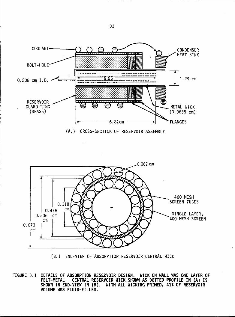
The metal-walled reservoir used for quantitative measurements of
reservoir function is shown in Figure 3.1. In detail (A) of Figure 3.1, an axial
cross section of the reservoir assembly is shown. The fluid absorption
wieking was a single layer of 0.0635 cm thick felt-metal on the reservoir
wall and a central cylindrical wick of 0.673 cm O.D. and 0.318 cm I.D. The
central wick assembly is shown in dotted profile in (A) and in cross section
in (B). The inside and outside diameters of the central wick are a single
layer of 400 mesh stainless screen. The internal screened tubes, used to
give the structure rigidity as well as a small priming radius, are also of
400 mesh screen and approximately 0.062 cm in diameter. Thirteen tubes were .
used on the inner layer and 21 tubes on the outer layer. The tubes were
sealed at the end facing the condenser and maintained open at the other end
to minimize bubble entrapment.
The entire reservoir is 6.81 cm long and 1.29 cm in diameter, and has
a 41% volumetric fluid load. Reservoir parameters needed for modeling are
given in Table 3.1.
33
COOLANT
BOLT-HOLE
0.206 cm I.D.
RESERVOIRGUARD RING(BRASS)
CONDENSERHEAT SINK
1.29 cm
METAL WICK(0.0635 cm)
FLANGES
(A.) CROSS-SECTION OF RESERVOIR ASSEMBLY
0.062 cm
0.3180.475 cm
0.536 cmcm
0.673cm
400 MESHSCREEN TUBES
SINGLE LAYER,400 MESH SCREEN
(B.) END-VIEW OF ABSORPTION RESERVOIR CENTRAL WICK
FIGURE 3.1 DETAILS OF ABSORPTION RESERVOIR DESIGN. WICK ON WALL WAS ONE LAYER OFFELT-METAL. CENTRAL RESERVOIR WICK SHOWN AS DOTTED PROFILE IN (A) ISSHOWN IN END-VIEW IN (B). WITH ALL WICKING PRIMED, 41* OF RESERVOIRVOLUME WAS FLUID-FILLED.

34
TABLE 3.1. RESERVOIR SPECIFICATIONS/CONDUCTANCE PARAMETERS
3Reservoir total volume 8.87 cm
Wick/f luid volume fraction (6r), (6C) 0.465, 0.0375
Fluid volume fraction in wick (nr)» (nc) 0.886, 0.68
Wick thickness 0.068 cm
Reservoir and heat sink temperature 11 - 13°C
Gc 0.0443 W/cmK
Heat pipe orientation 0.24 cm favor-able tilt
Reservoir guard ring and condenser sink both cooled by samewater circuit.
35
3.1.2 Testing Methods
All tests were made using methanol working fluid. The heat pipe was
initially loaded with methanol and set to 0.25 cm reflux tilt to ensure an
absence of fluid pooling in the condenser. Operation without noncondensable
gas for several hours was used to determine leak tightness. The nonconden-
sable gas was then inserted in sufficient quantity to allow gas control
operation over the highest temperature range. Several cycles of the heat
pipe from 10 to 25 watts appeared to stabilize heat pipe response, and this
may be related to priming of the liquid reservoir.
After stable response was obtained, data were gathered and gas sub-
sequently removed for heat pipe testing in a lower temperature range.
The absorption reservoir was used with the gases carbon dioxide,
ammonia, and butane. After the absorption reservoir test sequence was com-
pleted, the wicking was removed from the reservoir and testing with nitrogen
was used to define an experimental reference. Nitrogen has negligible
solubility in methanol, in the context of this study.
An operating run was also made with all gas removed and an isothermal
heat pipe to determine heat loss through the insulation package. Heat loss
is linear and given as
Qal = 0.0636 (Ty-Ta) (watts) (27)
where T is vapor temperature and T is ambient temperature. Heat loss via
the nylon screws to the heat sink is
Q£2 = 0.0226 (Ty-Ts) (watts) (28)
Data presented in Section 3.2 have been corrected for these two losses.

36
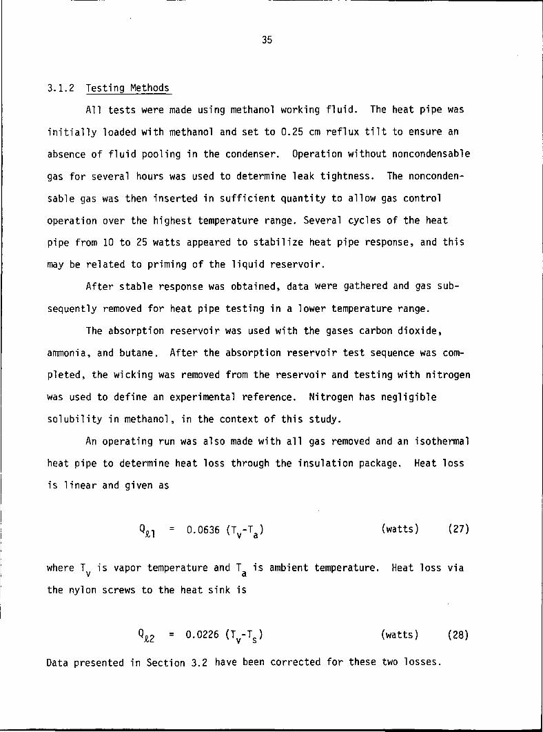
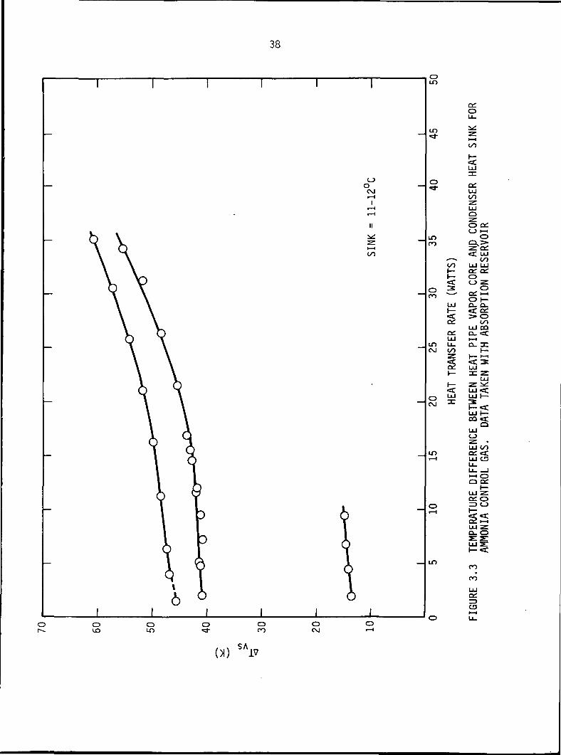
3.2 Experimental Results
Using the testing techniques given in Section 3.1.2, Figures 3.2 -
3.4 present the vapor-core heat-sink temperature difference, AT , as a function
of power level for the control gases Np, C(L, C4Hin' and NH3' As mentloned
earlier, the nitrogen data were taken with the liquid reservoir wieking
removed and hence represent a reference gas control design of equal reservoir
volume. The temperature control band with ammonia and butane as control
gases is less by about a factor of 2.5 relative to N2 for a nominal control
range of 5 to 20 watts. The experimentally determined control bands are
given in Table 3.2 for the gases used. The Ostwald solubility coefficient
is also given at the nominal reservoir temperature of 12.0°C.
3.3 Data Interpretation
3.3.1 Temperature Control
Table 3.2 presents a comparison of experimental and predicted
performance for both the absorption reservoir tests with CCL, C4Hin ancl NH3
and gas reservoir tests with nitrogen. In general, the gases C.H.Q and NH~
had, for a given heat transfer band-width, a temperature band-width 1/2 to
1/3 that seen with the standard gas reservoir and nitrogen. This difference
amounts to a saving in reservoir volume of a factor of 5 to 7.5.
The data comparison in Table 3.2 is based on AT/AQ. The heat pipe
vapor core temperature was found to be essentially linearly dependent on Q,
the heat transfer rate, provided that the gas front resided in the condenser.
Therefore, the control capability has been characterized on the basis of the
slope of the function T (Q). In each test, the slope AT/AQ was calculated by
a least-squares fit to the data over the linear region. The data have also

O
CMo
o o CO
oLO
CO
oco
LT> a:CM LU
<:LU
un
.ou_
coI—LU OL
O
LU ct.CO LU•z. coLU LUQ (V
LU CO01 coo <tC_5 u:o: I—O HH
LU Q. <C
<t
\— t—
LU O
LU CMLU O3 O
LU Oco •z.«tLUCJ O
Qi JLU <_}LU ILU CI—H
Q COLU
LU CO0£«tZD CD
LU
LU OI— O
CM
CO
LUC£13CD
oun oCO
oCM
00
38
oo
CM
00
LO
oo
Q;UJ00
o on<_) I—f
in oie£ LU
*-^ ooOO LU LUI— 0±0;I— O<C o z
O 3 ,0CO
inCM
oCVJ
Lf)
UJ
o: >-<o i—0.0.<c o;> o
ooLU COo. «Ct—IQ_ 1C
<C 3LU3T Z
LU
LU <LU I—
?<LU (—CO eC
OLUO
LU OO
LU CD
i OCC
on oZ5 O
o_ o
LT> coooLUo:
oLO
oro
oCM
39
ooCMi—tI
z>-Hto
oin
in
inCO
ro
in o£CM LU
LUOO
s
.-i a:CO HH
LU h- LUa: D. oooe LU0:00:LU into eo oo
Q LU
LU ZOf LU <O O «I CO
O Z C9O. LU Z< LU I-H
0- < I—I-H S OO. Z
toz •-< ceLU X »-iLU^O
Q£LUCOLUoe
CO
Z —I LULU o n:Of D£ I—LU h-U- Z •"U_ O QHH <_> LU0 S*zoLUo
LU
in
2 ceoLU O >-H
CO
LUQC
O
oin oco
oCM
oo

40
•M Om a)•i- jz> t—OJQ E
o+-> S-c u.O)u toi. 4J<D ro
CX. O
OC\JI
oo
O)
in c_>i— oco ro
cr
4-> I—IB <a
4-> Oin
ro
oi
en
coLO
coo
CM
OI
I—
OI
CTlo
oa:
CD U-o C3CO LLJ«=C a:
co ccO UJ•—i Q.rv* yet UJ> (—
or a:O t-tu_ o>- ex:fV I i Ict CO2: uj2: CECO <f.
•X. Q
QJ
IB
o a>oo
a>3
03 cr
inCM
naJ- <«-oi O
UJ ^iO- Qix o
C\J
CO
CO
cr<
OlQi
o+i
CO
roLO
O COin
"COLT>«=!- Oin
ino
CO
o
enCO
o
ooCMI
ino
CMo
incoCM
L^ f"^ f"^
cr> en"CM " i—I
CT> OCO
O OCO
OCMCM
\
ino
oCM
UD>—I
O VOin"CM
i—i .o-> or-1
O
inIB
CD
r—OS-
4_>co
C_3
OJO)0J_
-»->• z:
O)C XJO •!-
J3 XS- 0IB ••-
C_3 C^
O)cIB
4->3
CO
IB•^CO
O
<uO)
T3QJ
4J J-OJ -i-
« i-C 0)C7> W)•i- Ol10 CgO)
•O CO
T3 •«-S- •)->re ex•o s-c oIB (/>
0)oIB
OJ
i-oex03
01IBOl
IB
</) <C
II II<DtoIB
CO <C CQ
H CM

41
been organized by the nominal vapor-sink operating temperature difference
in the range 7.5 to 10.0 watts. The resulting data ranges, and the lengths
of the linear regions are approximately as follows
Region 1: ATvs @ 8.75 w = 22.5°C; linear span = 2.0 to 12.5 W
Region 2: ATy$ @ 8.75 w = 37.5°C; linear span = 2.5 to 15.0 W
Region 3: ATys (a 8.75 w = 50.0°C; linear span = 4.0 to 17.5 W
The experimental values of AT/AQ in Table 3.2 represent each temperature
region investigated. For comparison with calculated values of AT/AQ, the
individual values have been averaged. Both the averaged and individual
experimental values are presented in Figure 3.5 for relative comparison.
Control capability of the absorption reservoir is in qualitative
agreement with estimated values of AT/AQ using a flat-front model and the
dissolution models discussed in Section 2. The experimental control ratios
compare with theory as follows
AT/AQ for N2; 20% lower than theory
C02; 24% lower than theory
C4H1Q; 14% higher than theory
NH3; 100% higher than theory
The general experimental trend is a reduced effect of Ostwald coefficient
although performance improvements are still apparent as a increases.
Figure 3.6 shows the experimental data compared to predicted control ratios
for an Ostwald coefficient range from 1.0 to 1000.
The reduced influence of a beyond about 30 may be attributable to a
spreading out of the gas front because of high solubility. Condenser thermo-
couples indicated a considerably longer gas front with the three soluble
gases than with nitrogen. However, because of differences in molecular
42
^ ss sss
3
\— Z _J Ql«t _J LU3: on o
C0 2
or^ <JZ>
O
O
o
o*3-
ocooCSJ
o1-H
o
oo
Q LU <C(— LU > 0?O CO O LULU =3 £ O.u. LU z:u_ LU o: LU •LU Qi I— ID
UJ CDO 2 Z C\JLU I—i -z coi«: z »—•—• 3: co CD ZDS Z i—i t—< OS 2 CO COLU O LU «C»— zget
•> I—I>- ozo a:—I •—»— >0—i z»-« a: »—«*: «*3 LU ot— o co<cZ CO LU Lu
^cO^^ccSSh-^^LU CO CD CDa. «LUX CO h_ LU QLU LU O LU
CO Z Z <_>LU «£ LU LU =D3: CD CD Qi QI— O LU UJ
LU Qi Lu Q;Lu LU t— LUO OC I—i O£ CO
z z «<Zl- <3O LU«-i LU a: co -z.bF1-**0<r u_ _,ce co \-t~ • LU *£CO • Q > 3rs o >—i a: I—
i =3 LU O_J CO Z3
. _lLU LU
—j 3: e><: _i i— z t—CJ O >—i LU Z5
S^33:zQ. Z Q I— HH<C O LU >—itx o _j i—CD _1Q<
Z KH Z UJ<c o LU 3 3:
mcoLUIX
CD
IRA
bv
43
5.0
1.0
0.5
cr<J
0.10
0.05
MIN. TEMP.
MAX. TEMP
I1.0 10.0 100.0
OSTWALD COEFFICIENT
1000.0
FIGURE 3.6 RATE-OF-CHANGE OF VAPOR CORE TEMPERATURE WITH RESPECT TOHEAT INPUT FOR THE THREE SOLUBLE CONTROL GASES USED WITHMETHANOL WORKING FLUID. THE THEORETICAL INFLUENCE OFSOLUBILITY ON TEMPERATURE CONTROL IS ALSO SHOWN, ASSUMINGA SHARP GAS-VAPOR INTERFACE. THE BAND STRUCTURE REFLECTSMAX. OPERATING TEMPERATURE RANGE.
44
weight between the gases and working fluid vapor, vertical gravity-force
stratification of the gas front could produce the same broadening. Another
possibility is that small amounts of insoluble gas either leak into the
heat pipe via 0-rings or hydrogen is generated from water contained in the
methanol . The direct effect of this will be a reduction in control ratio
which becomes increasingly important as a increases in size. Further
investigation of this effect is warranted.
In summary, the temperature change resulting from a given heat input
change has been reduced by a factor of two to three for an absorption reservoir
of identical volume to a gas reservoir. This has been demonstrated
with a common gas-control heat pipe working fluid, methanol. Equivalent
performance with a wetted wall gas reservoir would require a volumetric
increase to about 5x to 7.5x the volume of the absorption reservoir.
3.3.2 Transient Response
Figure 3.7 presents experimental data on time response of vapor core
temperature to a step-increase in heat transfer rate from approximately 5
watts to 20 watts at a nominal vapor temperature of 55 C above sink temperature.
The vapor core temperature is nondimensionalized by defining
- Tvo~ - — ry—vm vm vo
where T is the initial vapor temperature and Tvm is the final vapor tempera-
ture. The experimental data do not show any significant effect of reservoir
design or control gas on transient response. However, various amounts of
over-shoot are analytically predicted for the absorption reservoir system
depending on the diffusion coefficient of the gas in the working fluid. The
<CLU
: LU <_) _j
LUi O _J I—: 1-1 <£. o
UJ
Q. a: oLU t— oo ;I— i—i i—11oo 3 a:
ooLU
O CD OI— O
C\JLU z OE:0- Oi—i »>U_a. •
QJ Z1— • 3«C -i- Ouj>-'n:z oo
C£a: i—i oi—i O OOo > _i> a: «feg LULU oo oo00 LU l—iLU a:
00 i-«I— oo
oo >-<z aSo*-3O£ O"
CJa:oo<ctD
LU
oo —: <C •-<> CD o
I— oO LU
O i—«
I— LU OHO. CJ LUo; z: ooO LU LUoo a: oiOQ LU<C U_ Z
LU OLU a: >—i:n i—|— LU Q.
o LU-LU LUa:Q- LU
CD111 rvOO etz: _iOa. >-oo o:LU LUGC. >
O 001Ll_ < r ,
LU O <t IOO IZ LU 3O OOa. z oOO O CMLU a.a: oo o
ooo
LUf-l . Lf)oo j—«Co;
coLUo:CO
Ooc
' a:p «: u. O
LUoo a:_l Z3LU ooO LU
46
diffusivity of ammonia gas in methanol is estimated to be 5 to 10 (10" )2
cm /sec. For this range of diffusivity, about a 40% over-shoot in dimension-
less temperature is predicted, while only a few percent was observed.
Butane gas also displayed minimal over-shoot and under-shoot.
Alternate explanations for this divergence in behavior remain to be
explored. It is possible that the high solubility of these gases in methanol
creates a turbulent mass transfer phenomena that is much more effective than
simple diffusion. However, if this is correct, then it must be determined
if these turbulent transfer processes will function in zero-g, since they
could require a gravity field.
An alternate explanation is that the diffuse gas front found for soluble
gas/liquid combinations is a function of both radial and axial position, so
that the absorption process and overall heat transfer coefficient are not
adequately described by a flat-front gas control model. Vertical stratifica-
tion of the gas front could also create experimental deviation from analytical
predictions.
Viability of the absorption reservoir technique has been demonstrated
on the basis of heat transfer. However, questions raised related to transient
response and gravity effects should be explored in further detail to fully
substantiate performance of the reservoir in a zero-g environment.
47
4.0 CONCLUSIONS
Significant improvements in thermal control have been experimentally
demonstrated for the absorption reservoir. With the same volume as a
reference gas reservoir, temperature control has been improved by a factor
of two to three for butane and ammonia control gases with methanol working0
fluid. A smaller improvement was shown for carbon dioxide, a gas with lower
solubility in methanol. Equivalent thermal performance from a gas reservoir
would require a volume 5 to 7.5 times that used with the absorption reservoir
and ammonia or butane. Detailed comparisons of absorption reservoir tests,
standard reservoir tests with equal volume, and theoretical predictions are
given in Table 3.2. Transient response was relatively unaffected by reservoir
design, and heat pipe response to a step-change in heat transfer rate was
very rapid.
However, this responsiveness is very interesting in that the experi-
mental heat pipe was expected to exhibit a relatively large transient
temperature over-shoot on the basis of diffusion rate constants for the
liquid absorption reservoir. Further analytical and experimental work is
needed to determine the basis for this unexpected performance improvement,
since the apparent improvement in mass transfer may be related to gravity-
assisted convection effects not present in zero-g.
In addition, temperature measurements on the outside of the condenser
indicated a very diffuse gas front in the case of the soluble gases ammonia,
butane, and carbon dioxide. The gas front was relatively sharp in the case
of nitrogen, which is relatively insoluble in methanol and very close in
molecular weight. A diffuse gas front and/or a front that is vertically
stratified because of gravity effects may partially account for the improved
48
gas control, independent of the soluble gas reservoir effect; the thermal
effects of nonperpendicular gas fronts are not well understood. It would be
of interest to redesign the test apparatus so that the heat pipe could be
operated in a vertical reflux position with a lower molecular weight gas
such as ammonia. In a vertical position, the ammonia-methanol vapor phase
mixture would effectively float on the lower density methanol vapor below.
By carefully comparing operating characteristics in both horizontal
and vertical modes, the effects of gravity on gas front shape could be
determined, and transient response behavior linked to either a gas-front
related-mechanism or reservoir mass transfer mechanism.
49
REFERENCES
1. E. W. Saaski, Condensation Heat Transfer in a Closed Tube Containing aSoluble, Noncondensable Gas. NASA Final Report CR 137811, December 1975.
2. E. W. Saaski, Investigation of Bubbles in Arterial Heat Pipes, NASACR 114 531, December 1972.
3. E. Thomsen and J. Gjaldbaek, Acta Chemica Scandannavica, Vol 17, 134 (1963)
4. W. Bowden, et al., J. Chem. Eng. Data. Vol. 11, No. 3, 296 (1966).
5. W. Hayduk and H. Laudie, AICHE J.. Vol. 19, No. 6, 1233 (1973).
6. M. lino, et al., J. Chem. Eng. Data. Vol. 15, No. 3, 446 (1970).
7. J. Chu, et al., Vapor-Liquid Equilibrium Data, J. W. Edwards Publ.,Ann Arbor, Michigan, 1956.
8. L. 0. Roellig and C. Geise, J. of Chem. Phys.. Vol. 37, No. 1, 114 (1962).
9. F. E. Karasz and G. D. Halsey, Jr., J. of Chem. Phys.. Vo. 29, No. 1,173 (1958).
10. E. Sinor and F. Kurata, J. of Ch. Eng. Data. Vol. 11, No. 4, 537 (1966).
11. R. J. Burch, J. of Ch. Eng. Data. Vol. 9, No. 1, 19 (1964).
12. A. L. Benham and D. L. Katz, AICHE J.. Vol. 3, No. 1, 33 (1957).
13. R. E. Latimer, AICHE J.. Vol. 3, No. 1, 75 (1957).
14. G. Armstrong, et al., J. Res. N.B.S., Vol. 55, No. 5, 265 (1955).
15. H. Cheung and D. Wang, I and EC Fund., Vol. e, No. 4, 355 (1964).
16. F. B. Sprow and J. M. Prausnitz, Cryogenics, December 1966, p. 338.
17. F. P. Ricci, Diffusion in Simple Liquids, Phys. Rev., Vol. 156, No. 1,184, 1967.

A-l
APPENDIX A
Diffusion From a Double-sided Slab
Given the physical system shown in Figure 2.6, it is desired to solve the
diffusion equation in one dimension
— = n d C ,-,n Dab 8X2 »>
A dimensionless distance and concentration are defined as
x* = TTX/JI (2)
C* = (C-C0)/(Cm-Co) (3)
Boundary conditions are assumed to be
@ t=0, C*=l for all x*
@ t=0+,C =0 for x*=0 and x*=ir
for t-*•», c =0 for all x*
The diffusion equation now becomes
O _ r\+ O \*
- - *
where
This has the Fourier sine series solution
D* - "ab
I bN EXP(-N2D*t) sin(Nx*) (5)
N=l
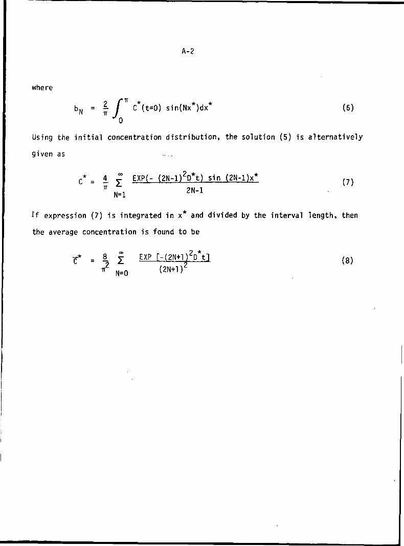
A-2
where
bN = | I C*(t=0) sin(Nx*)dx* (6)* 0
Using the initial concentration distribution, the solution (5) is alternatively
given as
C* = i £ EXP(- (2N-l)2D*t) sin (2N-l)x* (?)n ?N-1
N=l ^N i
If expression (7) is integrated in x* and divided by the interval length, then
the average concentration is found to be
- = 8 £ EXP [-(2N+l)2D*t1 {8)
•" N=0
g^Fl lfr-f ^^
* 6 ^> MAR 1992
RCH, DEVELOPMENT,
J SIGMA RESEARCH, IN2952 GEORGE WASHINGTON WAYRICHLAND, WASHINGTON 99352
D PLANNING, PHYSICS, BIOLOGY, AND MECHANICAL, CHEMICAL. AND OPTICAL ENGI