heat exchanger network self-optimising control
TRANSCRIPT
Heat exchanger network self-optimising control
Application to the crude unit at Mongstad refinery
Alexandre Leruth MSc. in Chemical Engineering
June 2012
2
Abstract
The master thesis is about operation of the heat exchanger network of a crude
unit at Mongstad refinery (Statoil). The network is such that the crude oil feed stream
is splitted in parallel branches made of shell and tube heat exchangers recovering heat
from distilled products. Optimal operation of the given network is defined as the
maximum achievable temperature of the crude oil outlet stream. In other words, it
means to maximise the overall heat transfer in the network.
This work applies the concept of self-optimising control for the operation of
the given network. The steady-state performances of the self-optimising variables
derived by Jäschke (Jäschke, 2012) are assessed and two main control configurations
are examined: a simple decentralised control configuration (PIDs Control) and an
advanced multivariable control configuration (Model Predictive Control). The steady-
state performances appears to be moderate but need to be re-assessed using a proper
steady-state model. The decentralised control configuration is found to present
acceptable dynamic performances while the advanced multivariable configuration only
enhances them a bit.

3
Table of Contents
1.Introduction .................................................................................................................................... 6
2.Heat exchanger network dynamic model ................................................................................ 8
2.1. Shell and tube heat exchangers ............................................................................................. 8
2.2. Heat exchanger model ............................................................................................................. 9
2.3. Network model ....................................................................................................................... 11
2.4. Data treatment ........................................................................................................................ 15
2.5. Simulation tools ...................................................................................................................... 26
2.6. Model analysis ........................................................................................................................ 29
3.Self-optimising variables ........................................................................................................... 34
3.1. Theorical framework ............................................................................................................. 34
3.2. Application to Heat exchanger network .......................................................................... 36
3.3. Application to the studied heat exchanger network ...................................................... 38
4.Steady-state performances ........................................................................................................ 39
4.1. Solving the network for given self-optimising variables ............................................. 39
4.2. Selection of JT variables for branches B & C .................................................................. 40
4.3. Optimal split fractions .......................................................................................................... 43
5.General features of the control configuration ..................................................................... 48
5.1. Objectives ................................................................................................................................. 48
5.2. Temperature measurements ................................................................................................ 49
5.3. Constrained case ..................................................................................................................... 49
5.4. Secundary split control on branch F ................................................................................. 50
5.5. SIMC tuning rules for PI(D) controllers ......................................................................... 51
5.6. Controlled variables .............................................................................................................. 55
6.Decentralised control ................................................................................................................ 56
6.1. Dynamics of the self-optimising variables ....................................................................... 56
6.2. Filters for feedforward control abatement ....................................................................... 58
6.3. PI controllers tuning ............................................................................................................. 62
6.4. Simulation results .................................................................................................................. 62
6.5. Decentralised control configuration without filters ...................................................... 66

4
7.Advanced multivariable control .............................................................................................. 68
7.1. Model linearization ................................................................................................................ 69
7.2. Model Predictive Controller tuning .................................................................................. 69
7.3. Comparative simulation results .......................................................................................... 70
8.The flow control case ................................................................................................................ 74
7.1. Model linearization ................................................................................................................ 74
7.2. Model Predictive Controller tuning .................................................................................. 74
7.3. Comparative simulation results ........................................................................................ 706
9.Conclusion .................................................................................................................................... 79
Bibliography .................................................................................................................................... 80
Appendix .......................................................................................................................................... 80
A. Data reconciliation – temperatures and flowrates ............................................................ 82
B. PI controllers tuning (valve control with filters) ............................................................. 87
C. MatLab© codes ......................................................................................................................... 92
5
Nomenclature
:
:
:
:
:
:
:
:
:
:
:
:
6
Chapter 1
Introduction
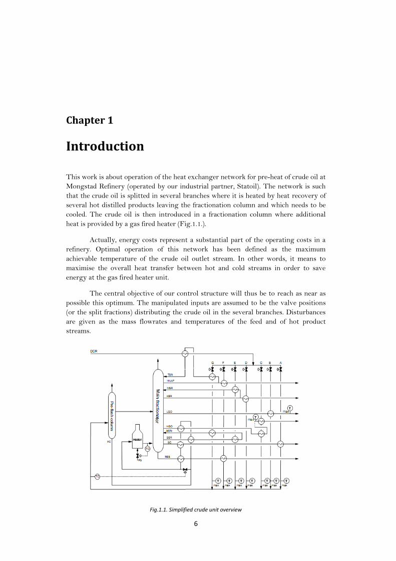
This work is about operation of the heat exchanger network for pre-heat of crude oil at
Mongstad Refinery (operated by our industrial partner, Statoil). The network is such
that the crude oil is splitted in several branches where it is heated by heat recovery of
several hot distilled products leaving the fractionation column and which needs to be
cooled. The crude oil is then introduced in a fractionation column where additional
heat is provided by a gas fired heater (Fig.1.1.).
Actually, energy costs represent a substantial part of the operating costs in a
refinery. Optimal operation of this network has been defined as the maximum
achievable temperature of the crude oil outlet stream. In other words, it means to
maximise the overall heat transfer between hot and cold streams in order to save
energy at the gas fired heater unit.
The central objective of our control structure will thus be to reach as near as
possible this optimum. The manipulated inputs are assumed to be the valve positions
(or the split fractions) distributing the crude oil in the several branches. Disturbances
are given as the mass flowrates and temperatures of the feed and of hot product
streams.
Fig.1.1. Simplified crude unit overview

7
Operation of heat exchanger networks is much less studied compared to their
design (Glemmestad et al., 1999). Bypass selection for control of heat exchanger
networks has been investigated (Mathisen et al., 1992). More considerations on utility
consumption then suggested a method that minimises it (Mathisen et al., 1994a). A
method based on repeated steady state optimization was presented (Boyaci et al., 1996)
and then a method for on-line optimisation and control of heat exchanger networks
has been also introduced (Aguilera and Marchetti, 1998).
In the Mongstad case, on-line optimisation has been implemented for the
operation (Lid, Strand and Skogestad, 2002). Steady-state mass and energy balance of
the whole network (20 heat exchangers) yields the process model. The model is fitted
by data reconciliation and optimal split fractions are computed. When implemented,
this system led to a 2% reduction in energy consumption. However, this method
requires many efforts from the operators.
Indeed, using real-time optimisation brings difficulties in building and
adapting accurate models for complex processes (Chachuat et al., 2009) and the
combination of steady state detection, parameter estimation, data reconcilation and
solving of a nonlinear optimisation problem online (White, 1997) is not very practical
for operations.
In this work, the idea of self-optimising control will be applied to the given
network. Self-optimising control offers to pursue economical objectives J without the
need of re-optimise the system when disturbances d occur. Actually, self-optimising
control (Skogestad, 2000) is achieved if a constant setpoint policy results in an
acceptable loss L. On the Figure 1.2., we see that a loss generally results when we keep
a constant setpoint rather than reoptimising when a disturbance occurs.
where (1.1)
Fig.1.2. Loss as a result of a constant setpoint policy
Jäschke (Jäschke, 2011) introduced invariants for optimal operation of process
systems which led to a patent application in the case of parallel heat exchangers
(Jäschke, 2012). This work follows the master thesis of Daniel Greiner Edvardsen
(Edvardsen, 2011) where a steady-state study using these invariants as self-optimising
variables showed very promising results.

8
Chapter 2
Heat exchanger network dynamic model
2.1. Shell and tube heat exchangers
The Mongstad preheat train is composed of shell and tube heat exchangers made of
steel. This is the more common type of heat exchanger in the petrochemical industry.
They handle large flowrates due to their high hydraulic diameter. One set of tubes
called the tube bundle contains the first fluid while the second fluid runs over the tubes
on the shell side so that heat can be transferred between them.
Shell and tube heat exchangers are typically used for high pressure
applications due to their shape which insure a strong mechanical resistance. We
distinguish many types of shell and tubes heat exchanger due to the diversity of
internal flow configurations. The most common are made of one, two or four passes on
the tube side and only one on the shell side.
Sinnott and Towler (Sinnott and Towler, 2009) presented some reasons for
using shell and tube exchangers:
- The configuration gives a large surface area in a small volume
- Good mechanical layout
- Well-established fabrication techniques
- Can be constructed from a wide range of materials
- Easily cleaned
- Well established design procedures

9
Fig. 2.1. Shell and tube Heat Exchanger (Alaquainc)
Baffles are used in shell and tube heat exchangers to lead the fluid on the shell side across the tube bundle. They are perpendicular to the shell and hold the bundle (Fig.2.1.). They also prevent the tubes from sagging and vibrating. Their influence on the flow mixing is to be considered in dynamics studies, especially in pure countercurrent heat exchangers (one pass on each side) which are the units in which the transfer is the most distributed.
With the time, the heat transfer capacity of such units in the crude oil preheat train may be reduced due to fouling. A well-known cause of fouling is asphaltene insolubility which may depose on the exchange areas.
2.2. Heat exchanger model
2.2.1. Topology and assumptions
A dynamic model of the heat exchanger network is needed in order to assess
controllability. The first step is to build a general dynamic model of shell and tube heat
exchanger. Following the work of Mathisen (Mathisen, 1994b), a flexible lumped
multicell model has been developed in order to involve all the important features such
as the number of compartments for each fluid (number of elements), fluid heat
capacities, heat transfer coefficients (including convective and wall resistances) and
wall capacitance.
Since flow configuration has not a major effect on the dynamics of the whole
network (Mathisen, 1994b), a counter-current multi-cell topology has been introduced.
As shown on the Figure 2.2., each internal fluid side is represented by a serie of N
elements of fixed volume.
10
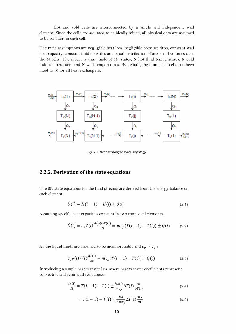
Hot and cold cells are interconnected by a single and independent wall
element. Since the cells are assumed to be ideally mixed, all physical data are assumed
to be constant in each cell.
The main assumptions are negligible heat loss, negligible pressure drop, constant wall
heat capacity, constant fluid densities and equal distribution of areas and volumes over
the N cells. The model is thus made of 3N states, N hot fluid temperatures, N cold
fluid temperatures and N wall temperatures. By default, the number of cells has been
fixed to 10 for all heat exchangers.
Fig. 2.2. Heat exchanger model topology
2.2.2. Derivation of the state equations
The 2N state equations for the fluid streams are derived from the energy balance on
each element:
(2.1)
Assuming specific heat capacities constant in two connected elements:
(2.2)
As the liquid fluids are assumed to be incompressible and :
(2.3)
Introducing a simple heat transfer law where heat transfer coefficients represent
convective and semi-wall resistances:
(2.4)
(2.5)

11
The N state equations for the wall elements are easily obtained by energy balance :
(2.6)
2.3. Network model
The process flow diagram of the Mongstad crude oil preheat train is shown below
(Fig. 2.3.). All streams are assumed to be in a complete liquid phase. The crude oil
enters the network at the point ln1 and is distributed in seven branches
A,B,C,D,E,F,G. The heat exchangers are represented in grey while the measurements
points (temperature and/or flowrate) are indicated by a circle, white for the crude oil,
colored for the hot streams.
The first part of this project was to prepare a model in order to control as best
as possible the distribution of the crude oil in the network, focusing on the several
branches. Since the self-optimising variables have so far been developed only for
parallal branches that split from one single point and gather in another single point,
the sub-network indicated by the red box has been studied in this work. This sub-
network consists of 6 branches from A to F and 11 heat exchangers involved in the
crude oil heating.
The rest of the network is a scheme quite similar to serie structure so the
direct objective of the control strategy is different than finding an optimal distribution
of the crude oil in several branches. Consequently, this second sub-network has less
degree of freedom and offers less possibilities of control which could influence the final
temperature. However, a study on this second sub-network or, at least, on its
influences to the first sub-network will be required to implement successfully the self-
optimising control method. This is left as future work.
The heat exchanger network that will be modeled in this project can be
described as it is shown on the simplified process flow diagram shown in Figure 2.4.

12
Fig. 2.3. Statoil Mongstad crude unit Heat Exchanger Network
Fig.2.4. Simplified process flow diagram

13
2.3.1. Global energy balance
When the crude oil has been heated by the several branches of the heat exchanger
network, the crude oil streams are gathered in a mixer and the outlet total temperature
can be computed with the energy balance.
(2.7)
(2.8)
(2.9)
The formula for the heat capacities is introduced in the section 2.4.2. Data treatment,
heat capacities.
(2.10)
(2.11)
where (2.12)
This amount of energy can then be expressed as a function of the unkown outlet total
temperature :
(2.13)
(2.14)
(2.15)
We can then calculate combining the equations (2.11) and (2.15):
(2.16)
This is a second order equation:
where
(2.17)

14
The physical solution is the temperature which will be positive, we expect the outlet
temperature to be around 150-250°C.
(2.18)
(2.19)
2.3.2. Distribution valve model
The distribution of the crude oil flow in the branches is assumed to be analogous to the
distribution of the electric current in a circuit of parallel resistances. Each branch of
the heat exchanger network comprises a valve providing resistance to the total inlet
crude oil flow (Fig. 2.5.). This resistance is assumed to be the inverse of the valve
position (opening fraction). The resistance (or pressure drop) of the heat exchangers is
assumed to be more or less the same in each branch and is not taken into account.
Fig. 2.5. Distribution valve model
The manipulated variables in our control problem are the valve positions:
(2.20)
So the crude oil feed flowrate in the branch i is calculated by the formula:
(2.21)
At optimal conditions, the branch having the highest feed flowrate should have its
valve fully open. Otherwise, the pressure drop could be reduced in the whole network.
This ascertainment will be taken into account for the design of the control structure.

15
2.4. Data treatment
In this project, data were provided by Statoil Mongstad and needed to be selected and
treated appropriately while some unkown values had to be estimated. This section
presents the steps between the data reception and the data introduction in our shell
and tube heat exchanger network model.
2.4.1. Volumes and Areas
Fortunately, all heat exchanger areas were provided in the data files received from
Statoil Mongstad. These values have been directly introduced in the models without
any modification.
Unfortunately, some heat exchanger bundle and shell volumes were not
provided in the data files received from Mongstad. Simple linear correlations based on
the known heat exchangers data have been examined in order to find the best way to
estimate the missing data. Similarities between the heat exchangers have been
observed and we thus hope that the estimated data is reasonable.
Fig. 2.6. Correlation for missing bundle volume estimations
R² = 0,9518
y = 3986,6x + 234,99
0
2000
4000
6000
8000
10000
12000
14000
16000
0 0,5 1 1,5 2 2,5 3 3,5 4
Bu
nd
le W
eig
ht
[kg]
Bundle volume [m^3]
Correlation

16
Fig. 2.7. Correlation for missing shell volume estimations
The best correlations (maximum coefficient of determination) were obtained
between the bundle weight and the bundle volume (Fig. 2.6.) and between the bundle
weight and the shell volume (Fig. 2.7.). So we used these two correlations in order to
estimate the missing volumes (in italic in the table 2.18.).
Heat
exchanger
Exchange
Area [m²]
Bundle
Volume
[m^3]
Shell
Volume
[m^3]
Bundle
Weight
[kg]
Shell
Weight
[kg]
Crude
flow
side
A1 138 0,8 1,7 3760 5450 Shell
B1 162 0,714 1,287 3080 7430 Shell
B2 203 0,962 1,727 4070 3840 Tube
C1 264 1,4 2,38 5480 7020 Tube
C2 233 1,153 2,059 4830 4890 Tube
D1 260 1,25 1,86 4910 4970 Tube
D2 313 1,88 2,61 6400 8450 Shell
E1 164 0,7 1,2 3060 3170 Tube
F1 77 0,45 0,67 1580 2420 Tube
F2 278 1,39 2,5 5520 6130 Tube
F3 278 1,33 2,53 5610 6390 Tube
Tab. 2.8. Heat exchangers data
y = 2289,9x + 116,1
R² = 0,9742
0
2000
4000
6000
8000
10000
12000
14000
16000
0 1 2 3 4 5 6 7
Bu
nd
le W
eig
ht
[kg]
Shell Volume [m^3]
Correlation
17
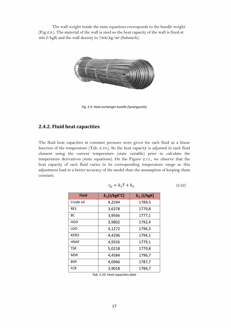
The wall weight inside the state equations corresponds to the bundle weight
(Fig.2.9.). The material of the wall is steel so the heat capacity of the wall is fixed at
460 J/kgK and the wall density to 7800 kg/m3 (Substech).
Fig. 2.9. Heat exchanger bundle (Synergycoils)
2.4.2. Fluid heat capacities
The fluid heat capacities at constant pressure were given for each fluid as a linear
function of the temperature (Tab. 2.10.). So the heat capacity is adjusted in each fluid
element using the current temperature (state variable) prior to calculate the
temperature derivatives (state equations). On the Figure 2.11., we observe that the
heat capacity of each fluid varies in its corresponding temperature range so this
adjustment lead to a better accuracy of the model than the assumption of keeping them
constant.
(2.22)
Fluid [J/kgK°C] [J/kgK]
Crude oil 4,2594 1789,5
RES 3,6378 1779,8
BC 3,9566 1777,1
HGO 3,9802 1792,4
LGO 4,1272 1796,3
KERO 4,4296 1794,1
HNAF 4,9326 1779,1
TSR 5,0218 1779,8
MSR 4,4584 1796,7
BSR 4,0966 1787,7
FCR 3,9018 1784,7
Tab. 2.10. Heat capacities data

18
Fig.2.11. Heat capacities as a function of temperature
2.4.3. Temperatures and flowrates
The temperatures and flowrates of the network have been given by Statoil Mongstad.
Production measurements between the 23 october 2011 at 13:07:25 and 24 october
2011 at 13:06:26 on a 1 minute basis have been provided. Looking at the variations on
the feed temperature and other measurements, the values used for the model were
collected at a point of time where the network seems to be the most stabilised,
especially in a thermal perspective (Fig.2.12., red arrow): the 23 october 2011 at
18:10:36.
Fig. 2.12. Production feed temperature variations
124,2 124,4 124,6 124,8
125 125,2 125,4 125,6 125,8
23/10/2011 12:00:00 24/10/2011 00:00:00 24/10/2011 12:00:00
Time
Feed Temperature [°C]
100 120 140 160 180 200 220 240 260 280 3002000
2200
2400
2600
2800
3000
3200
3400
Temperature [°C]
Heat
capacity [
J/k
gK
]
cpcrude
cpres
cpbc
cphgo
cplgo
cpkero
cphnaf
cptsr
cpmsr
cpbsr
cpfcr

19
Mass and energy balances have been used to estimate unkown temperatures
and flowrates (some useful streams data are not present in the list provided by Statoil)
and simple form of data reconciliation has been used to modify the given
measurements as little as possible in order to fulfill the stationary mass and energy
balances.
In order to simplify the problem, we assumed the uncertainties on the
flowrates to be two times higher in percentage than the temperature uncertainties (in
percentage on a Celsius temperature scale basis). Actually, we observe that flowrates
vary a lot in operations and they may differ a lot compared to steady-state. For
simplicity, we also assumed the crude oil feed temperature to be fixed (not subject to
reconciliation) and the network crude oil outlet temperature to be not given as a data.
Actually, if the desired values for the model differs from the given data, it is
probably much more due to the fact that the given data come from ongoing production
with all kind of transient effects in the network (different time scales). The
measurement errors are probably the main secondary source of deviations.
The data treatment for temperatures and flowrates is detailed branch per
branch in the appendix. Nevertheless, we illustrate it here for branch F. Please refer to
the simplified process flow diagram (Fig. 2.4.) for the notations.
- Heat exchanger F1 :
(2.23)
(2.24)
(2.25)
- Heat exchanger F2 :
(2.26)
(2.27)
(2.28)

20
- Heat exchanger F3 :
(2.29)
(2.30)
(2.31)
In these balances, we have all the data except for which is easily determined by the
mass balance:
(2.32)
However, introducing the data (Tab 2.13.), the equations do not match perfectly so
reconciliation is needed to obtain steady-state values.
252,54 125,00 136,957 194,664 153,96 72,738
205,699 244,379 172,484 113,146 119,41
199,086 172,207 109,10 133,13 Tab. 2.13. Branch F data
For the given values, we observe that:
(2.33)
(2.34)
(2.35)
So we introduce a first reconciliation factor such that:
(2.36)
(2.37)
(2.38)
(2.39)
(2.40)
(2.41)
(2.42)

21
We optimise the sum of the energy balance absolute errors for (using Microsoft
Excel Solver) and obtain:
(2.43)
(2.44)
(2.45)
So we introduce a second reconciliation factors such that:
(2.46)
(2.47)
We optimise again the sum of energy balance absolute errors and obtain:
(2.48)
(2.49)
(2.50)
So we finally introduce a third reconciliation variable such that:
(2.51)
(2.52)
(2.53)
(2.54)
And we solve the previous energy balances with the new temperatures and flowrates
in order to find ε, and :
(2.55)
The reconciled values are listed in Tab. 2.14. :
253,60 125,00 137,535 193,843 154,610 72,125
205,759 244,379 172,534 113,081 119,91
199,028 170,953 110,689 133,69 Tab. 2.14. Branch F reconciled values

22
2.4.4. Fluid Densities
The following table 2.15. has been provided by Statoil Mongstad. The density is given
is kg/dm3.
Temp [°C] Crude Residue BPA HGO MPA LGO KERO HNA TPA
15 0,845 0,935 0,874 0,893 0,825 0,859 0,827 0,792 0,788
50 0,821 0,916
100 0,788 0,89 0,823 0,844 0,768 0,805 0,77 0,73 0,7204
150 0,75 0,864
200 0,707 0,837 0,759 0,786 0,69 0,737 0,694 0,64 0,631
250 0,657 0,81 0,724 0,754
300 0,598 0,782 0,684 0,72 0,587 0,66 0,593 0,513 0,499
350
0,751 0,639 0,689
Tab. 2.15. Density data
This leads to the Figure 2.16. We observe clearly the results of the crude oil
fractionation separating the products according to their volatility (which is related to
the density).
Fig. 2.16. Fluid densities as function of the temperature
Considering the range of temperature for which each fluid is concerned, we
find out that the assumption of constant density required by the model is quite strong.
Nevertheless, for each fluid, we fix the density value at the arithmetic mean in the
temperature range using linear interpolation.
0,4
0,5
0,6
0,7
0,8
0,9
1
0 100 200 300 400
De
nsi
ty [
kg/d
m^3
]
Temperature [°C]
Crude oil
RES
BPA
HGO
MPA
LGO
KERO
HNA
TPA

23
Since we do not have densities for the fluid BC, we assume this fluid to be
similar to BPA (=BSR). Actually, BC is similar to BSR in respect the heat capacity
values (cfr. Fig. 2.11.) and is also described as a product in the bottom of the
fractionation column in Figure.1.1.
The results are shown in the table below.
Fluid Mean temperature [°C] Density [kg/m3]
Crude oil 166,33 735,96
Residue (=RES) 207,6659 832,86
BPA (=BSR) 256,221 719,023
HGO 195,0137 788,892
MPA (=MSR ) 199,6211 690,296
LGO 223,4688 718,929
KERO 211,1618 682,727
HNA 174,2267 663,196
BC 231,5176 736,938 Fig. 2.17. Fluid densities
2.4.5. Heat transfer coefficients
The heat transfer coefficients are the last unkown model variables and are estimated
separately for each heat exchanger unit by fitting the modeled heat transfer to the
reconciled heat transfer. Actually, the overall heat transfer in each heat exchanger is a
single variable to be adjusted so we introduced a single variable coefficient by unit. We
thus assume the heat transfer coefficient to be the same value on both streams (hot and
cold).
As said previously, this simplified heat coefficient includes convective and wall
resistances. That’s why its value should normally be a bit higher than what can be
found in the literature for physical heat coefficients (using heat transfer correlations).
The global heat exchanger heat transfer coefficient U can be simply estimated:
(2.56)
For liquid-liquid heat exchange, we can expect the U values in the range 150-
1200 W/m²K (Lunsford, 1998) so we expect h values in the range 300-2400 W/m²K.
The heat exchanger state variables are initialised with linear temperature
profiles and each branch is simulated separately and the heat transfer coefficients are
easily adjusted manually to obtain the steady-state reconciled heat transfer calculated
previously (Fig. 2.18.).

24
Fig. 2.18. Steady-state matching of the heat transfer, unit F1
The heat transfer coefficients values from this simulation procedure are listed in table
below (Table 2.19.).
Heat exchanger Heat transfer coefficient h [W/m²K]
A 1902
B1 1189
B2 713
C1 1565
C2 1565
D1 1250
D2 382.5
E 1976
F1 1381
F2 1462.5
F3 1257.5
Tab. 2.19. Heat transfer coefficients
Once the heat transfer coefficients are tuned, we can re-write the initialization
MatLab© file for the temperature profiles by extracting them out of each heat
exchanger with a sufficient simulation time for system to stabilise to its stationary
point.
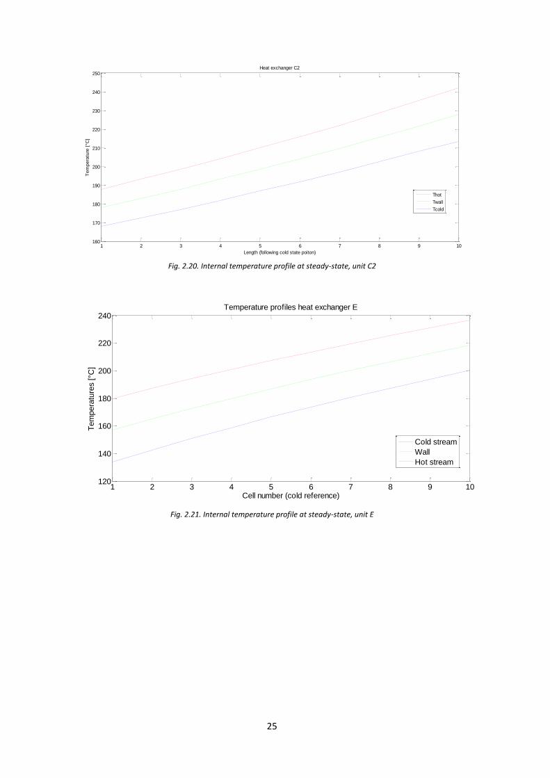
The temperatures profiles obtained are close to the linear profiles (Fig. 2.20 & 2.21).
400 600 800 1000 1200 1400 1600
135
140
145
150
155
160
165
170
Heat transfer coefficient [W/m2K]
Outlet te
mpera
ture
s [°C
]
Cold stream
Hot stream
25
Fig. 2.20. Internal temperature profile at steady-state, unit C2
Fig. 2.21. Internal temperature profile at steady-state, unit E
1 2 3 4 5 6 7 8 9 10160
170
180
190
200
210
220
230
240
250
Length (following cold state poiton)
Tem
pera
ture
[°C
]
Heat exchanger C2
Thot
Twall
Tcold
1 2 3 4 5 6 7 8 9 10120
140
160
180
200
220
240Temperature profiles heat exchanger E
Cell number (cold reference)
Tem
pera
ture
s [°C
]
Cold stream
Wall
Hot stream
26
2.5. Simulation tools
The software used in this project is exclusively MatLab© – Simulink which
offers both flexibility in implementation and strong solving capacities. Simulink is an
appropriate environment for this project. It provides an interactive graphical
environment and a customizable set of blocks libraries useful for design, simulation,
implementation and testing of time-varying systems including control.
2.5.1. S-function
The shell and tube heat exchanger model has been introduced in Simulink as a
S-function (system-function). This mechanism offers to extend the capabilities of the
Simulink environment. So an S-function is a computer language description of a
Simulink block written in MatLab© or in C, C++, Fortran. S-functions are
dynamically linked subroutines that the MatLab© interpreter can automatically load
and execute.
Actually, S-functions use a special calling syntax called the S-function API
that enables to interact with the Simulink engine. This interaction is very similar to
the interaction that takes place between the engine and built-in Simulink blocks. S-
functions follow a general form and can accommodate continuous, discrete, and hybrid
systems. (MatLab©)
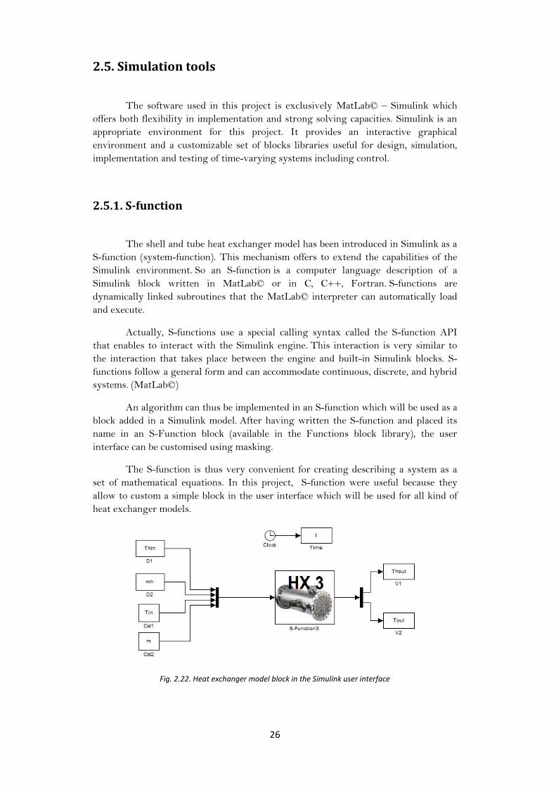
An algorithm can thus be implemented in an S-function which will be used as a
block added in a Simulink model. After having written the S-function and placed its
name in an S-Function block (available in the Functions block library), the user
interface can be customised using masking.
The S-function is thus very convenient for creating describing a system as a
set of mathematical equations. In this project, S-function were useful because they
allow to custom a simple block in the user interface which will be used for all kind of
heat exchanger models.
Fig. 2.22. Heat exchanger model block in the Simulink user interface
27
It is possible to specify parameter values to be passed to the s-functions using
the S-Function block S-function parameters. The order in which the function requires
them is to be respected. The parameter values can be constants, names of variables
defined in the MatLab© or model workspace, or MatLab© expressions.
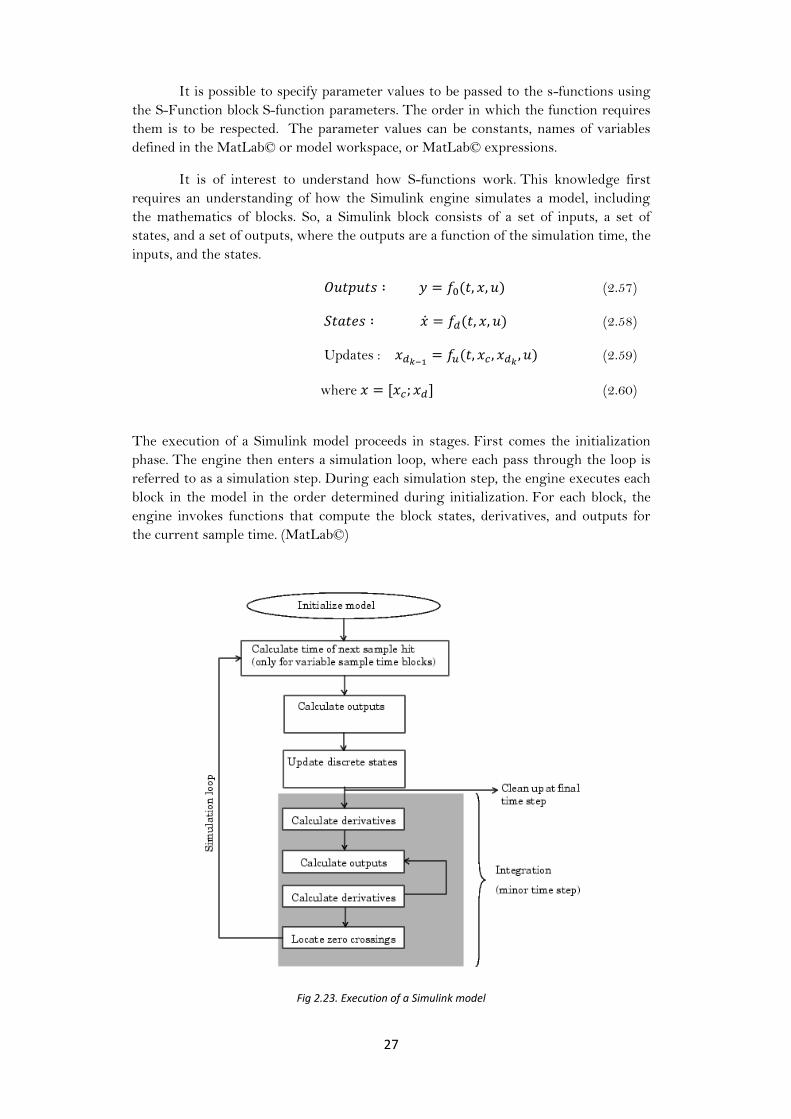
It is of interest to understand how S-functions work. This knowledge first
requires an understanding of how the Simulink engine simulates a model, including
the mathematics of blocks. So, a Simulink block consists of a set of inputs, a set of
states, and a set of outputs, where the outputs are a function of the simulation time, the
inputs, and the states.
(2.57)
(2.58)
Updates : (2.59)
where (2.60)
The execution of a Simulink model proceeds in stages. First comes the initialization
phase. The engine then enters a simulation loop, where each pass through the loop is
referred to as a simulation step. During each simulation step, the engine executes each
block in the model in the order determined during initialization. For each block, the
engine invokes functions that compute the block states, derivatives, and outputs for
the current sample time. (MatLab©)
Fig 2.23. Execution of a Simulink model

28
The inner integration loop takes place only if the model contains continuous
states. The engine executes this loop until the solver reaches the desired accuracy for
the state computations. The entire simulation loop then continues until the simulation
is complete. (MatLab©)
During simulation of a model, at each simulation stage, the Simulink engine
calls the appropriate methods for each S-Function block in the model. Tasks
performed by S-function callback methods include:
Initialization :
- Initializing a simulation structure that contains information about the S-
function
- Setting the number and dimensions of input and output ports
- Setting the block sample times
- Allocating storage areas
Calculation of next sample hit :
- For a variable sample time block, the next step size is calculated
Calculation of outputs in the major time step:
- All the block output ports are valid for the current time step
Update of discrete states in the major time step:
- Once-per-time-step activities such as updating discrete states
Integration:
- The engine calls the output and derivative or zero-crossing portions of the S-
function at minor time steps and so the solvers can compute the state or locate the
zero crossings. (MatLab©)
A useful concept in s-function is the presence of the flags that directs the
engine to the appropriate code in the several steps of the execution. In case of direct
feedthrough (the output is controlled directly by the value of an input port signal), a
special flag can be used to detect algebraic loops which may force the simulation
results of the S-function to not converge. (MatLab©)

29
2.6. Model analysis
It is of great importance to verify that the heat exchanger network dynamic model is
physically coherent. We thus have to analyse how the model behaves in respect to
what we would expect from the real plant, especially in the time-scale dynamics for
which we want to design a new control configuration.
2.6.1. Heat Exchanger model analysis Exchanger A is taken as an example.
Step change in a inlet temperature:
At time = 20s, the hot stream inlet temperature passes from 295.45°C to
245.45°C. The heat transfer is reduced and both outlet temperatures drops as
expected. The outlet temperature of the cold stream (blue) has a fast response due to
the counter-current flow configuration. The outlet temperature of the hot stream (red)
has a delayed response due to the sojourn time in the heat exchanger. (Fig.2.24)
Fig.2.24. Step change in the hot stream inlet temperature
Step change in a inlet flowrate:
At time = 20s, the hot stream flowrate passes from 15.91 kg/s to 18.91 kg/s.
We notice the direct change on the hot outlet temperature induced by the assumption
of incompressibility. The heat transfer grows as expected. For each stream, the
characteristic time of the dynamic response is very close to the sojourn time in the heat
exchanger (58.9s for the crude oil; 37s for the hot fluid). (Fig. 2.25)
Fig. 2.25. Step change in the hot stream flowrate
0 50 100 150 200 250 300140
160
180
200
220
240
Time [s]
Tem
peatu
re [
°C]
ToutA
ThoutA
0 50 100 150 200 250 300160
180
200
220
240
Time [s]
Tem
pera
ture
[°C
]
ToutA
ThoutA

30
2.6.2. Branch model analysis The Branch C, constituted of two heat exchangers in serie, is taken as example.
Step change in an inlet temperature:
At time=100s, the hot stream inlet temperature passes from 248.77°C to
298.77°C. The two exchangers have together such a capacity for heat transfer that the
last temperature of the hot streams (outlet of C1) has changed of 7,5°C only. The heat
transfer has been reduced, in both heat exchangers with almost the same intensity. We
clearly observe the slow dynamics on the heat exchanger C1 due to the capacity of the
heat exchanger C2. (Fig. 2.26)
Fig. 2.26. Step change in the hot stream inlet temperature
Step change in an inlet flowrate:
At time=100s, the hot stream flowrate passes from 26.97 kg/s to 20.97 kg/s.
We observe that the temperature of the hot fluids reduces very much in the heat
exchanger C2 (the first to be crossed by the hot fluid) so the heat transfer on this unit
tends to be conserved. The heat transfer reduces mainly on the heat exchanger C1 at
lower temperatures where the temperature difference is lower. This is due to the lower
driving force in the heat transfer. We observe that the temperature difference between
hot and cold fluid diminishes on the first heat exchanger while it grows on the second
one. (Fig 2.27)
Fig.2.27 Step change in hot stream flowrate
0 100 200 300 400 500 600 700 800120
140
160
180
200
220
Time [s]
Tem
pera
ture
[°C
]
ToutC2
ThoutC2
ToutC1
ThoutC1
0 100 200 300 400 500 600 700 800140
160
180
200
220
240
260
Time [s]
Te
mp
era
ture
[°C
]
ToutC2
ThoutC2
ToutC1
ThoutC1

31
2.6.3. Heat exchanger Network Model Analysis The complete model is examined in Simulink.
Step change in the feed temperature:
At time=100s, the feed temperature passes from 125°C to 150°C. The fastest
branch is E, then comes B, D, A and F, and finally C. The hot fluid flowrate of the
branch C is very low compare to the crude oil flowrate. The temperature profiles in
this branch thus are very narrow. After the step change, some heat of the crude oil is
even taken by the hot fluid branch at the outlet of the first heat exchanger. This
explains the observed slow dynamics. (Fig. 2.28)
Fig. 2.28. Step change in the feed temperature – Branches dynamics
The effect on the total outlet temperature of the crude oil is plotted on Figure
2.29. The temperature grows is of 7°C only so the heat transfer has been reduced as
expected (less driving force in the heat exchangers). The global dynamics of the
network is observed to be quite fast but realistic. (Fig. 2.29)
Fig. 2.29. Step change in the feed temperature – Outlet temperature dynamics
0 100 200 300 400 500 600206
208
210
212
214
216
Time [s]
Te
mp
era
ture
[°C
]
0 100 200 300 400 500 600200
210
220
230
240
Time [s]
Tem
pera
ture
[°C
]
ToutA
ToutB
ToutC
ToutD
ToutE
ToutF
32
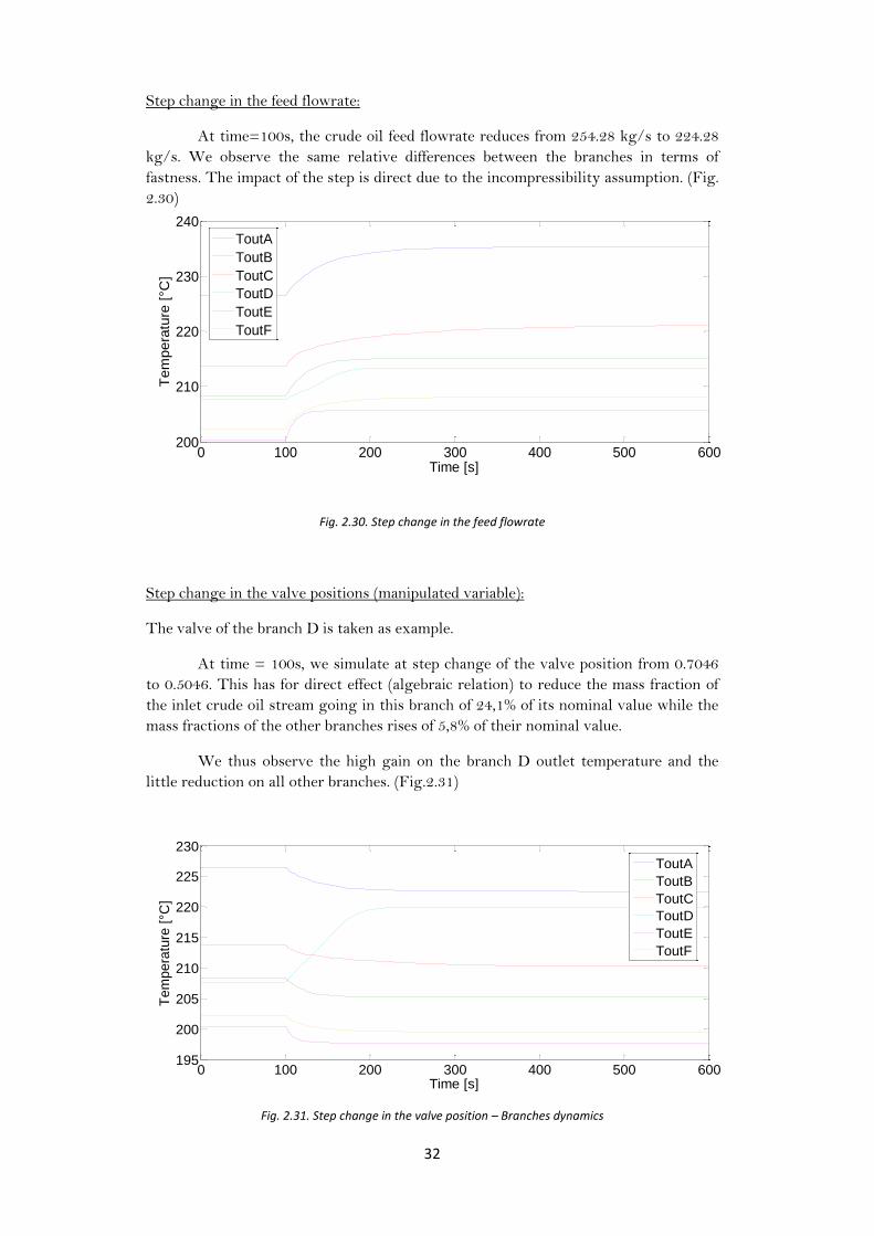
Step change in the feed flowrate:
At time=100s, the crude oil feed flowrate reduces from 254.28 kg/s to 224.28
kg/s. We observe the same relative differences between the branches in terms of
fastness. The impact of the step is direct due to the incompressibility assumption. (Fig.
2.30)
Fig. 2.30. Step change in the feed flowrate
Step change in the valve positions (manipulated variable):
The valve of the branch D is taken as example.
At time = 100s, we simulate at step change of the valve position from 0.7046
to 0.5046. This has for direct effect (algebraic relation) to reduce the mass fraction of
the inlet crude oil stream going in this branch of 24,1% of its nominal value while the
mass fractions of the other branches rises of 5,8% of their nominal value.
We thus observe the high gain on the branch D outlet temperature and the
little reduction on all other branches. (Fig.2.31)
Fig. 2.31. Step change in the valve position – Branches dynamics
0 100 200 300 400 500 600195
200
205
210
215
220
225
230
Time [s]
Tem
pera
ture
[°C
]
ToutA
ToutB
ToutC
ToutD
ToutE
ToutF
0 100 200 300 400 500 600200
210
220
230
240
Time [s]
Te
mp
era
ture
[°C
]
ToutA
ToutB
ToutC
ToutD
ToutE
ToutF

33
The response of total outlet temperature shows clearly the effect of the time-scale
separation between the branches. (Fig. 2.31)
Fig. 2.31. Step change in the valve position - Outlet temperature dynamics
2.6.4. Remark
Modeling is always connected to objectives. The dynamic differences between
each heat exchanger unit or branch in the network is clearly observed in our
simulation results. We expect these differences to be the main physical characteristic
of the system which needs to be handled by the control structure. The given model is
thus believed to be accurate, robust and flexible enough for a large study of possible
control configurations.
0 100 200 300 400 500 600206
206.5
207
207.5
208
Time [s]
Tem
pera
ture
[°C
]

34
Chapter 3
Self-optimising variables
3.1. Theorical framework
In the general case, the controlled variables are selected as functions of the
measurements. Experience and intuition still plays a major role in the design of
controlled system. However, the controlled variables used in this work have been
derived by a systematic approach. This approach associates the overall control
objectives with the selection of the controlled variables. (Jäschke, 2011).
3.1.1. Self-optimising control
Self-optimising control is when near-optimal operation is achieved with constant
setpoints for the controlled variables. The introduction to this concept presented here
is taken from Skogestad (Skogestad, 2004). Self-optimising control offers to not re-
optimise the system when disturbance occurs.
The general optimisation problem is to minimise a certain objective function subject to
some constraints:
(3.1)
(3.2)
Where J is the objective function, x represents the state variables, ut the manipulated
variables (available degrees of freedom) and d the disturbances. The equality
constraints g include the model equations and the inequality constraint are used to
respect the physics of the system (positive temperatures and mass flows for example).
Some of the inequality constraints h are often active constraints and must be equal to
zero. These constraints should be controlled with a corresponding number of degrees
of freedom.

35
Our problem is to decide what to control with the remaining degrees of freedom, u. If
the states x are eliminated using the model equations g the remaining unconstrained
problem is:
(3.3)
where is to be found and is the optimal value of the objective function.
We want to find a subset of the measured variables named c to keep constant at the
optimal values . Ideally, should be insensitive to the disturbances d to obtain
optimal operation. In reality, we aim at operation close to optimal and there is a loss
associated with keeping the controlled variable constant. This loss can be expressed as:
(3.4)
To select the controlled variables, the following guidelines presented by Skogestad
(2000) can be used :
- should be insensitive to disturbances
- should be easy to measure and control accurately
- should be sensitive to change in the manipulated variable (degree of freedom)
- For cases with more than one unconstrained degrees of freedom, the selected
controlled variables should be independent
These guidelines offer to reduce the effect of disturbances and reduce the
implementation error.
An ideal self-optimising variable, proposed among others by Halvorsen and Skogestad
(1997), is the gradient of the objective function:
(3.5)
which should be zero to ensure optimal operation for all disturbances. However,
measurement of the gradient is usually not available, and computing it requires
knowing the value of unmeasured disturbances. To find which variables are the best to
keep constant (approximations of the gradient), different approaches can be used:
- Exact local method
- Direct evaluation of loss for all disturbances (“brute force”)
- Maximum (scaled) gain method
- Null space method

36
3.2. Application to Heat exchanger network
Jäschke (Jäschke, 2012) applied his theorical work (Jäschke, 2011) on heat exchanger
networks made of parallel branches for which the objective function is easily defined as
the end temperature. The optimisation problem is:
(3.6)
(3.7)
Where g is the steady state model of the heat exchanger network and u the
available degrees of freedom. It is assumed that the hot streams are disturbances and
not degrees of freedom, hence the number of degrees of freedom is equal to the number
of splits in the heat exchanger network. In this work, the theory has been applied to
heat exchangers where no phase change happens as it is the case in our heat exchanger
network.
The work of Jäschke is subjected to a patent application while this work is
subjected to be sent to an industrial partner. Consequently, we present the expression
of the self-optimising variables without further development. The only major
assumption made by Jäschke in its derivation has been to approximate heat transfers
using the arithmetic mean temperature instead of the logarithmic mean temperature.
3.2.1. Branches composed of single heat exchangers
The controlled variable is:
(3.8)
where:
(3.9)
Fig. 3.1. Branches composed of single heat exchangers
Hence, for a heat exchanger network with two heat exchangers in parallel (Fig. 3.1.)
five measurements are need to achieve self-optimising control. Two measurement are
needed for each heat exchanger (outlet cold temperature and inlet hot temperature) in
addition to the feed temperature of the network.

37
3.2.2. Branches composed of two heat exchangers in series
Fig. 3.2. Two heat exchangers in series on branch 1
The controlled variable is:
(3.10)
where:
(3.11)
The ratio
has been identified to be a key variable for branches made of a single
heat exchanger.
In the same way, the formula
is identified to be a key
variable for branches made of two heat exchangers (index : 1 – 2) in series.
This variables will henceforth been introduced as self-optimising variables or Jäschke
Temperatures [JT]. Their dimension is the one of a temperature interval so their
physical unit is the Kelvin [K].
We observe that the expression (3.10) reduces the the expression (3.8) if (no
effect of the first heat exchanger) or if (no effect of the second heat
exchanger).

38
3.3. Application to the studied heat exchanger network Reproducing Fig.2.4. Simplified process flow diagram
The last section led to key variables for each branch for which the equality is leading
the network very close to optimal operation. Keeping the same notation introduced in
the section 3.2., here are the self-optimising variables which will be used for control in
this work.
(3.12)
The branches B and C of our studied heat exchanger network are made of two
heat exchangers in series using the same hot stream. They led us to consider also the
self-optimising variables (3.13) and (3.14) and select the best one according the steady-
state results.
(3.13)
(3.14)
39
Chapter 4
Steady-state performances
4.1. Solving the network for given self-optimising variables
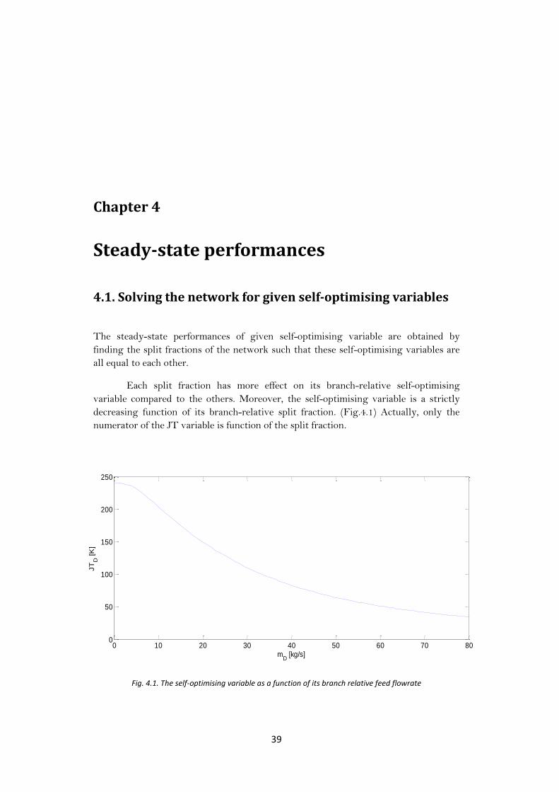
The steady-state performances of given self-optimising variable are obtained by
finding the split fractions of the network such that these self-optimising variables are
all equal to each other.
Each split fraction has more effect on its branch-relative self-optimising
variable compared to the others. Moreover, the self-optimising variable is a strictly
decreasing function of its branch-relative split fraction. (Fig.4.1) Actually, only the
numerator of the JT variable is function of the split fraction.
Fig. 4.1. The self-optimising variable as a function of its branch relative feed flowrate
0 10 20 30 40 50 60 70 800
50
100
150
200
250
mD
[kg/s]
JT
D [K
]
40
In order to respect the constraint on the mass balance, the split fraction of
branch F is defined as a result of the other split fractions. We introduce the variables:
(4.1)
The algorithm process is straightforward. As long as the variables are not
all sufficiently close to zero (<10-6 K), the branch-relative split fraction of the variable
having the higher absolute value is adjusted. This simple algorithm converges very
fast if a progressive tolerance scheme is adopted. The code can be seen in the appendix.
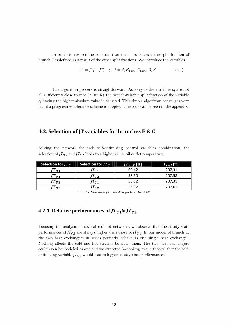
4.2. Selection of JT variables for branches B & C
Solving the network for each self-optimising control variables combination, the
selection of and leads to a higher crude oil outlet temperature.
Selection for Selection for [K] [°C]
60,42 207,31
58,60 207,58
58,02 207,31
56,32 207,61 Tab. 4.2. Selection of JT variables for branches B&C
4.2.1. Relative performances of &
Focusing the analysis on several reduced networks, we observe that the steady-state
performances of are always higher than those of . In our model of branch C,
the two heat exchangers in series perfectly behave as one single heat exchanger.
Nothing affects the cold and hot streams between them. The two heat exchangers
could even be modeled as one and we expected (according to the theory) that the self-
optimizing variable would lead to higher steady-state performances.
41
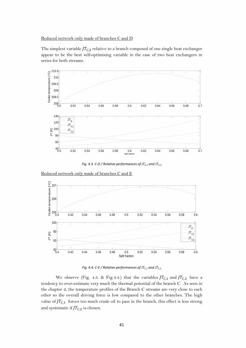
Reduced network only made of branches C and D
The simplest variable relative to a branch composed of one single heat exchanger
appear to be the best self-optimising variable in the case of two heat exchangers in
series for both streams.
Fig. 4.3. C-D / Relative performances of JTC,1 and JTC,2
Reduced network only made of branches C and E
Fig. 4.4. C-E / Relative performances of JTC,1 and JTC,2
We observe (Fig. 4.3. & Fig.4.4.) that the variables and have a
tendency to over-estimate very much the thermal potential of the branch C. As seen in
the chapter 2, the temperature profiles of the Branch C streams are very close to each
other so the overall driving force is low compared to the other branches. The high
value of forces too much crude oil to pass in the branch, this effect is less strong
and systematic if is chosen.
0.5 0.52 0.54 0.56 0.58 0.6 0.62 0.64 0.66 0.68 0.7208
208.5
209
209.5
210
210.5
Ou
tle
t te
mp
era
ture
[°C
]
0.5 0.52 0.54 0.56 0.58 0.6 0.62 0.64 0.66 0.68 0.740
60
80
100
120
140
Split fraction
JT
[K
]
JTD
JTC1
JTC2
0.4 0.42 0.44 0.46 0.48 0.5 0.52 0.54 0.56 0.58 0.6205
206
207
Ou
tle
t te
mp
era
ture
[°C
]
0.4 0.42 0.44 0.46 0.48 0.5 0.52 0.54 0.56 0.58 0.640
60
80
100
Split fraction
JT
[K
]
JTE
JTC1
JTC2

42
4.2.2. Relative performances of &
Focusing the analysis on several reduced networks, we observe that the relative
steady-state performances of , change from network to network and cannot
be presented as a general result.
Reduced network only made of branches A and B:
(4.2)
(4.3)
Fig. 4.5. A-B / Relative performances of JTB,1 and JTB,2
In this case (Fig. 4.5.), lead to a slightly higher outlet temperature than
. On the branch B, a part of the hot stream leaving the heat exchanger B2 do not
enter the first heat exchanger B1. The two heat exchangers in series cannot be
properly assumed to show the same physical characteristics as a single heat exchanger.
0.3 0.31 0.32 0.33 0.34 0.35 0.36 0.37 0.38 0.39 0.4213.7
213.8
213.9
214
214.1
214.2
214.3
Outlet
Tem
pera
ture
[°C
]
0.3 0.31 0.32 0.33 0.34 0.35 0.36 0.37 0.38 0.39 0.4-30
-20
-10
0
10
20
30
Split fraction
CV
s [
K]
cV1
cV2
43
4.3. Optimal split fractions
4.3.1. Calculation procedure
The steady-state performances of the self-optimising variable are better examined by
comparison to what is optimal to achieve in the network. A procedure to find the
optimal split fraction is needed. As for section 4.1., an algorithm using the variables
and the split fractions except one (branch F) will be used.
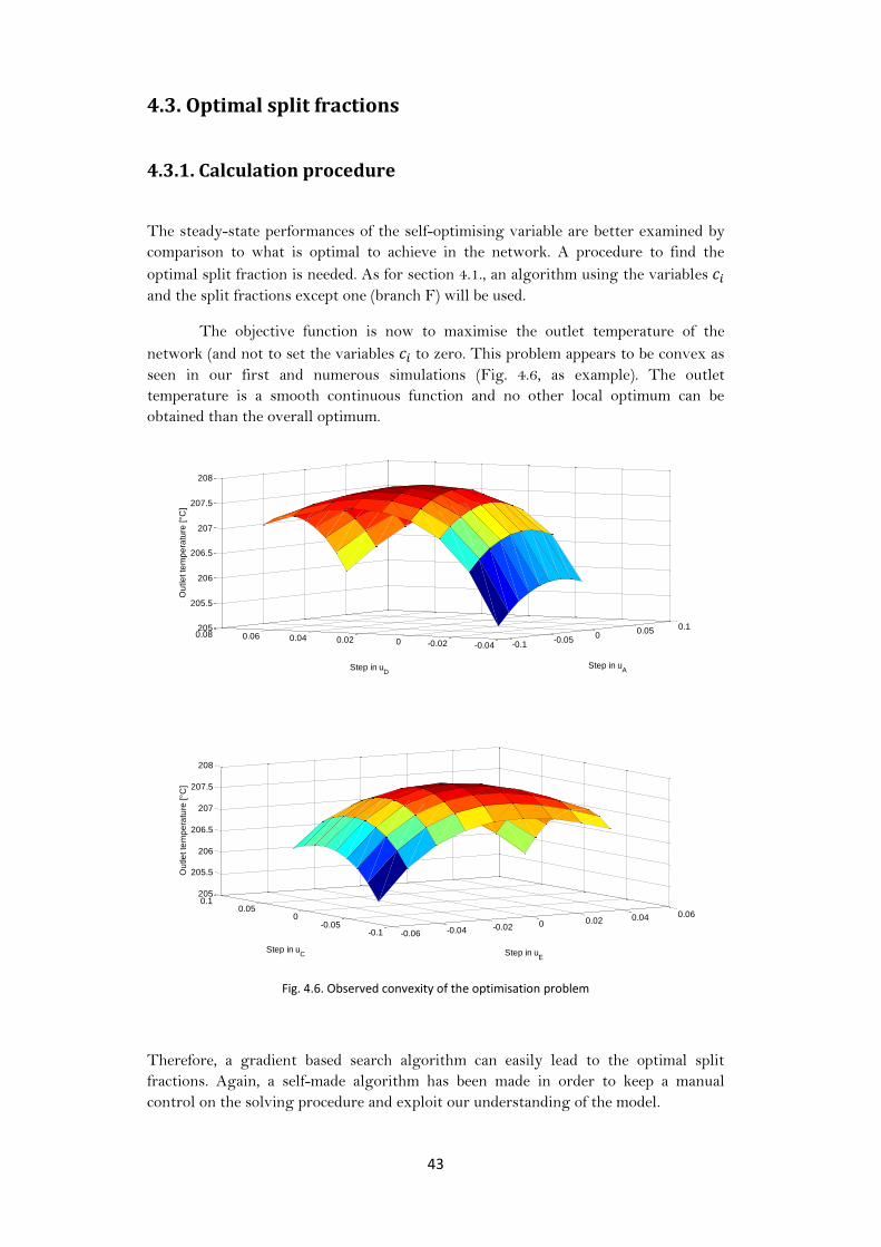
The objective function is now to maximise the outlet temperature of the
network (and not to set the variables to zero. This problem appears to be convex as
seen in our first and numerous simulations (Fig. 4.6, as example). The outlet
temperature is a smooth continuous function and no other local optimum can be
obtained than the overall optimum.
Fig. 4.6. Observed convexity of the optimisation problem
Therefore, a gradient based search algorithm can easily lead to the optimal split
fractions. Again, a self-made algorithm has been made in order to keep a manual
control on the solving procedure and exploit our understanding of the model.
-0.1-0.05
00.05
0.1
-0.04-0.0200.020.040.060.08205
205.5
206
206.5
207
207.5
208
Step in uAStep in u
D
Ou
tle
t te
mp
era
ture
[°C
]
-0.06 -0.04 -0.02 0 0.02 0.04 0.06
-0.1-0.05
00.05
0.1205
205.5
206
206.5
207
207.5
208
Step in uE
Step in uC
Ou
tle
t te
mp
era
ture
[°C
]

44
The principle used is very simple and allow the network to converge very fast. As long
as the local gradient is not close enough to zero, the algorithm looks for the optimal
point in the gradient direction by adapting the searching step according the results.
The code of the self-made algorithm can be found in the appendix D (MatLab© file
optim.m).
4.3.2. Results
The split fractions, crude oil outlet temperatures of each branch and the values of the
self-optimising variables are compared in three comparative cases: initial conditions (or
initial split), optimal conditions (or optimal split) and self-optimising conditions (or
self-optimising split). (Tab. 4.7) The initial conditions corresponds to the split
fractions as initialised in the model based on the data received from the operation
(where real-time optimisation is achieved) and their reconciliation as presented in
chapter 2.
Outlet
Temperatures [°C]
Initial split Optimal split Self-optimising
split
Branch A 226,455 228,452 222,98
Branch B 208,298 211,779 214,69
Branch C 213,673 217,49 208,49
Branch D 207,679 201,44 202,41
Branch E 200,279 200,39 206,03
Branch F 202,218 203,545 202,93
Network 207,65 207,79 207,61
Tab. 4.7. Outlet temperatures
Fig. 4.8. Outlet temperatures
125
135
145
155
165
175
185
195
205
215
225
ToutA ToutB ToutC ToutD ToutE ToutF Ttot
Tem
pe
ratu
res
[°C
]
Initial conditions
Optimal conditions
Self-optimizing conditions

45
Although the self-optimising conditions introduce some change in the distribution of
the crude oil in the network, the network outlet temperature stays at a high value and
very close to the optimum. (Fig. 4.8. & 4.9.) This can be explained by the flatness of
the optimum.
Fig. 4.9. Split fractions
Fig. 4.10. Self-optimising variables
We observe that the self-optimising variables are not strictly equal at optimum. This
may open a door for a “practical” adjustement of their expression (for example, in the
form of a non-theorical additional term which could use more process information than
simple temperature measurements). Such an adjustement will not be suggested here
and this is left as an idea for further work in order to improve the self-optimising
variables steady-state performances.
0
0,05
0,1
0,15
0,2
0,25
0,3
uA uB uC uD uE uF
Split
fra
ctio
ns
Initial conditions
Optimal conditions
Self-optimizing conditions
0
10
20
30
40
50
60
70
80
JTA JTB JTC JTD JTE JTF
JT [
K]
Initial conditions
Optimal conditions
Self-optimizing conditions

46
For single disturbances in the heat exchanger network (tab.4.11), there is almost no
gain using self-optimising control since the constant split (computed by the real-time
optimiser in the base case) still provides a higher outlet temperature in many cases.
Both constant split and self-optimising split stays relatively close to the optimum.
Disturbance on hot streams Outlet temperatures [°C]
Constant split Optimal
split
Self-optimising
split
Base case (No disturb.) 207,65 207,79 207,61
-10% flowrate – Branch C 206,94 207,18 206,98
+10% flowrate – Branch C 208,25 208,37 208,21
-10% flowrate – Branch F (HX F2&F3 hot stream)
206,89 207,07 206,88
+10 flowrates – Branch D 207,87 208,05 207,87
-10°C inlet – Branch C 206,70 206,86 206,72
+10°C inlet – Branch C 208,61 208,74 208,52
-10°C inlet – Branch B 206,64 206,81 206,62
+10°C inlet – Branch E 208,53 208,67 208,51
Tab. 4.11. Steady-state performances – single disturbance
If disturbances are combined on several branches then the constant split could
be far for the optimum split while the self-optimising split still stays relatively close to
it. However, as seen in table 4.12, if the hot streams flowrates on branches A,C,E are
reduced by 5% while the hot streams flowrates on B,D,F grow by 5%, the constant
split still provide a competitive outlet temperature.
Disturbance on hot streams
-5% on flowrates : A,C,E
+5% on floxrates : B,D,F
Constant split Optimal
split
Self-optimising
split
Split fractions
A 0,0837 0,0773 0,0847
B 0,1745 0,1681 0,1585
C 0,1315 0,117 0,1369
D 0,1952 0,2265 0,222
E 0,138 0,1331 0,1181
F 0,2771 0,278 0,2798
Outlet temperature [°C] 207,65 207,86 207,65
Tab. 4.12. Steady-state performances – Combined disturbances 5% flow
Finally, if the hot streams flowrates on branches A,C,E grows this time by 10%
of their nominal value while the hot streams flowrates on B,D,F are reduced by 10%,
the self-optimising split is now making a small positive difference (table 4.13).
The self-optimising variables cannot provide better steady-state performances
than the constant split given by the Real-Time Optimiser in the case of small
disturbances.

47
For major combined disturbances, the steady-state performances of the self-
optimising variables give a guarantee for the heat exchanger network to stay relatively
close to the optimum while a constant split could differ a lot from it. If the network is
subjected to such major disturbances (performance drift of the heat exchangers for
example) then the use of self-optimising control could be justified. (tab. 4.13,4.14,4.15)
Disturbance on hot streams
+10% on flowrates : A,C,E
-10% on floxrates : B,D,F
Constant split Optimal
split
Self-optimising
split
Split fractions
A 0,0837 0,0894 0,0947
B 0,1745 0,1545 0,1485
C 0,1315 0,1367 0,1561
D 0,1952 0,2189 0,2145
E 0,138 0,1472 0,1273
F 0,2771 0,2533 0,2589
Outlet temperature [°C] 207,25 207,45 207,27
Tab. 4.13. Steady-state performances – Combined disturbances 10% flow
Disturbance on hot streams -5% onflowrates& +5°C : A,C,E
+5% on flowrates & -5°C : B,D,F
Constant split Optimal
split
Self-optimising
split
Split fractions
A 0,0837 0,0754 0,082
B 0,1745 0,1696 0,1609
C 0,1315 0,1144 0,1316
D 0,1952 0,2306 0,2272
E 0,138 0,1276 0,1117
F 0,2771 0,2824 0,2866
Outlet temperature [°C] 208,64 208,92 208,73
Tab. 4.14. Steady-state performances – Combined disturbances 5% flow &5°C
Disturbance on hot streams +10% on flowrates & -10°C : A,C,E
-10% on flowrates &+10°C: B,D,F
Constant split Optimal
split
Self-optimising
split
Split fractions
A 0,0837 0,0939 0,1007
B 0,1745 0,1515 0,1433
C 0,1315 0,1429 0,1678
D 0,1952 0,2091 0,2031
E 0,138 0,1589 0,1404
F 0,2771 0,2437 0,2447
Outlet temperature [°C] 205,65 205,97 205,75
Tab. 4.15. Steady-state performances – Combined disturbances 10%flow &10°C
Note that the steady-state performances have been evaluated using a model build for a
study on dynamics. For further work, the author suggests to build an accurate steady-
state model in order to validate (or not) the given results and these statements.

48
Chapter 5
General features of the control configuration
5.1. Objectives
The control system based on the self-optimising approach pursues an economical
objective. In comparison to a control system for stabilization, control for economics is
usually taken into account in the upper layers of the control system made of the most
advanced controllers (multivariable, RTO). These upper layers then communicate
setpoints to the stabilizing layer, usually made of more simple controllers (PID)
(Skogestad and Postletwhaite, 2005).
The self-optimising control approach suggests using a single integrated layer
where economic self-optimising variables do not change with disturbances and prices.
In our work, we thus aim at controlling the heat exchanger network with a single
control layer. We look forward to a control configuration which will smoothly operate
the valve positions in order to pursue the equality of the self-optimising variables.
Steep changes, inverse responses and oscillations should be limited as much as
possible.
Fig. 5.1. General control configuration for a single valve position
49
5.2. Temperature measurements
All temperature are assumed to be measured with a sensor device for which the
dynamics is approximated by a simple first-order transfer function having time
constant of 5 seconds including a delay of 1 second.
(5.1)
5.3. Constrained case
By default, the operation of the heat exchanger network has been seen through the
single objective of heating the crude oil as much as possible (unconstrained problem).
It is possible that the operation of some heat exchangers of the network is constrained
by a setpoint on the hot stream side (fixed duty or temperature outlet).
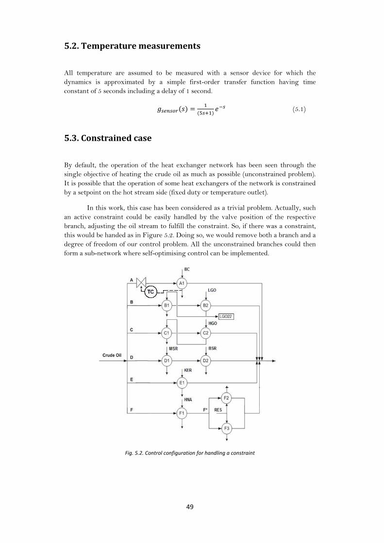
In this work, this case has been considered as a trivial problem. Actually, such
an active constraint could be easily handled by the valve position of the respective
branch, adjusting the oil stream to fulfill the constraint. So, if there was a constraint,
this would be handed as in Figure 5.2. Doing so, we would remove both a branch and a
degree of freedom of our control problem. All the unconstrained branches could then
form a sub-network where self-optimising control can be implemented.
Fig. 5.2. Control configuration for handling a constraint

50
5.4. Secondary split on branch F
On the branch F after the first heat exchanger is there a subdivision of the crude oil
stream where two heat exchangers in parallel are used to recover heat from the same
hot source. Moreover, these two heat exchangers have very similar physical
characteristics (volumes, areas, heat transfer coefficient).
The distribution of the crude oil between them is thus not expected to vary a
lot. Whatever the disturbance on the crude oil or on the hot stream, the split fraction
should stay close to 0,5. Consequently, we observe that the distribution of the crude
oil would not have major effect on the branch F crude oil outlet temperature and of
course even less on the network outlet crude oil temperature.
Fig.5.3. Outlet temperatures as a function of the split fraction F*
Even though a constant split would be sufficient, the self-optimising control
methodology could be implemented on this internal part of the network.
The valve positions of the crude oil on each sub-branch would be the
manipulated variables and algebraically would determine the split fraction (cfr. section
2.3.2.). The valve position of the sub-branch passed by the highest flowrate would be
automatically set to 1. The control structure would result in modifying the other one.
A PI controller would be used to do so.
The controlled variable would be:
(5.2)
(5.3)
Obviously, so the controlled variable could simply be :
(5.4)
0.2 0.3 0.4 0.5 0.6 0.7 0.8192
194
196
198
200
202
204
206
208
Split fraction F*
Ou
tle
t cru
de
oil
tem
pe
ratu
re [°C
]
Branch F
Network
51
5.5. SIMC tuning rules for PI(D) controllers Brief summary of the SIMC tuning (Skogestad, 2003)
The SIMC tuning rules of a PI(D) controller expressed in its series form :
(5.5)
The first step in the controller design procedure is to obtain from the original model
an approximate first (or second) order model including time delay in the form :
(5.6)
The model information such as the plant gain (k), the dominant lag time constant (
and the delay ( ) can be found in two ways :
- estimation based on the open-loop step response
- identification from the original transfer function (half-rule, approximations if needed)
Then, the idea is to specify the desired close-loop response (method named direct
synthesis for setpoints). We thus solve the close-loop system equation for the
corresponding controller :
(5.7)
Since we desire a simple first-order response with time constant (single parameter
for our controller):
(5.8)
Therefore, introducing a first-order Taylor series approximation of the delay:
(5.9)
(5.10)
This is a PID controller (5.5) for which :
(5.11)
This PID-setting was derived by considering only the setpoint response and
disturbance rejection can be improved by modifying the integral time for lag dominant
processes ( .

52
Analysing the close-loop characteristic polynomial in the case of a PI-controller :
1+
(5.12)
(5.13)
(5.14)
Oscillation occurs for
(5.15)
So a robust choice is to take
(5.16)
To summarise for all processes, we keep the tuning rule :
(5.17)
53
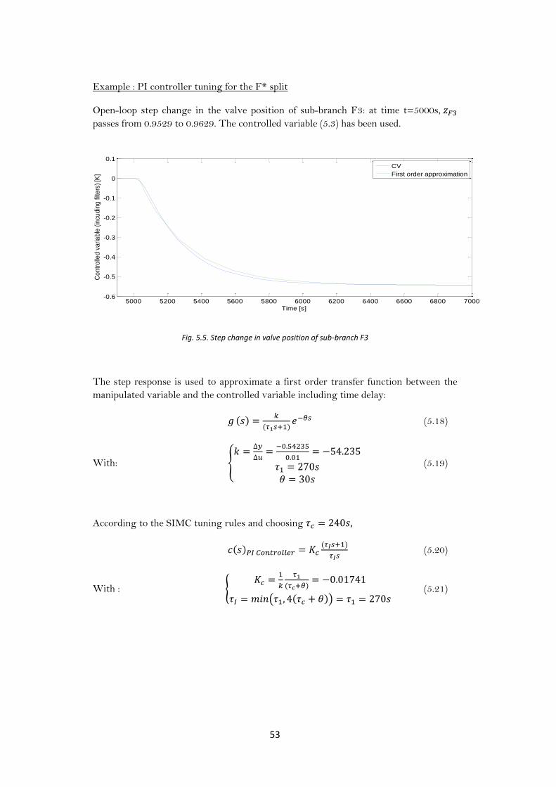
Example : PI controller tuning for the F* split
Open-loop step change in the valve position of sub-branch F3: at time t=5000s,
passes from 0.9529 to 0.9629. The controlled variable (5.3) has been used.
Fig. 5.5. Step change in valve position of sub-branch F3
The step response is used to approximate a first order transfer function between the
manipulated variable and the controlled variable including time delay:
(5.18)
With:
(5.19)
According to the SIMC tuning rules and choosing
(5.20)
With :
(5.21)
5000 5200 5400 5600 5800 6000 6200 6400 6600 6800 7000-0.6
-0.5
-0.4
-0.3
-0.2
-0.1
0
0.1
Time [s]
Co
ntr
olle
d v
aria
ble
(in
cud
ing
filte
rs)
[K]
CV
First order approximation

54
Close-loop simulation results
At time t=4000s, the crude oil inlet temperature passes from 125°C to 135°C.
At time t=5000s, the hot stream inlet temperature passes from 244,38°C to 234,38°C.
At time t=6000s, the crude oil flowrate passes from 70,45 kg/s to 59,88 kg/s.
At time t=7000s, the hot stream flowrate passes from 62,16 kg/s to 74,59 kg/s.
Fig. 5.6. Close –loop simultation – Outlet temperatures
The implemented control has no distinguishable effects on the branch
dynamics, as desired. (Fig. 5.6) On the graph, we notice the fastest responses of the
heat exchanger F2 due to its slightly larger heat transfer coefficient.
The valve position F2 stays to 1 since the sub-branch F2 keeps a higher crude
oil flowrate than the sub-branch F3. The changes on the valve position F3 are smooth
as desired. (Fig.5.7)
Fig. 5.7. Close-loop simulation – Valve operation F3
4000 4500 5000 5500 6000 6500 7000 7500 8000198
200
202
204
206
208
210
Time [s]
Ou
tle
t te
mp
era
ture
s [°C
]
Tout
F2
Tout
F3
Tout
Branch F
4000 4500 5000 5500 6000 6500 7000 7500 80000.936
0.938
0.94
0.942
0.944
0.946
0.948
0.95
0.952
0.954
0.956
Time [s]
Va
lve
Po
sitio
n F
3
55
5.6. Controlled variables
In the section 2.3.2., the branch valve positions have been introduced as our
manipulated variables. In order to reduce the pressure drop as much as possible, it has
been observed that the branch having the highest crude oil flowrate should always
have its valve fully open. In the nominal conditions, it is the branch F. All our control
structures will thus focus on manipulating the other valve positions and set, by default,
the valve on branch F fully open.
If there is such a disturbance in the system that the self-optimising variables
requires lead to a higher flowrate on another branch than branch F, the corresponding
valve position will saturate (being fully open) without being able to grow the crude oil
flowrate anymore.
In order to avoid this saturation effect, the values given by the controllers for
the valve positions [ ] will be artificially allowed to pass the value 1. These values
will then be algebraically treated in such a way that the highest will be set to 1 and the
others proportionally adjusted in order to get back a physical sense [ ].
(5.22)
(5.23)
The control structure will have to adjust the variables
. In order to do so, the following simple combinations of the
self-optimising variables will be used:
(5.24)
Actually, the self-optimising variable on each branch need to be taken into
account. The special role played by the one of the biggest branch [ ] is believed to
provide high robustness due to the higher capacity of this branch (inertia effect) and its
lowest tendency to be strongly affected by steep changes in the whole network. Good
dynamic performances are thus expected to result.
56
Chapter 6
Decentralised control
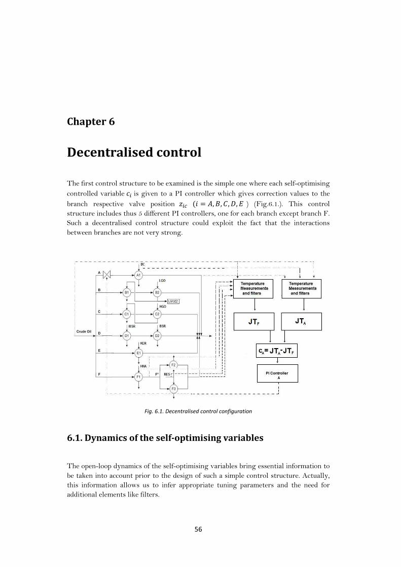
The first control structure to be examined is the simple one where each self-optimising
controlled variable is given to a PI controller which gives correction values to the
branch respective valve position ) (Fig.6.1.). This control
structure includes thus 5 different PI controllers, one for each branch except branch F.
Such a decentralised control structure could exploit the fact that the interactions
between branches are not very strong.
Fig. 6.1. Decentralised control configuration
6.1. Dynamics of the self-optimising variables
The open-loop dynamics of the self-optimising variables bring essential information to
be taken into account prior to the design of such a simple control structure. Actually,
this information allows us to infer appropriate tuning parameters and the need for
additional elements like filters.
57
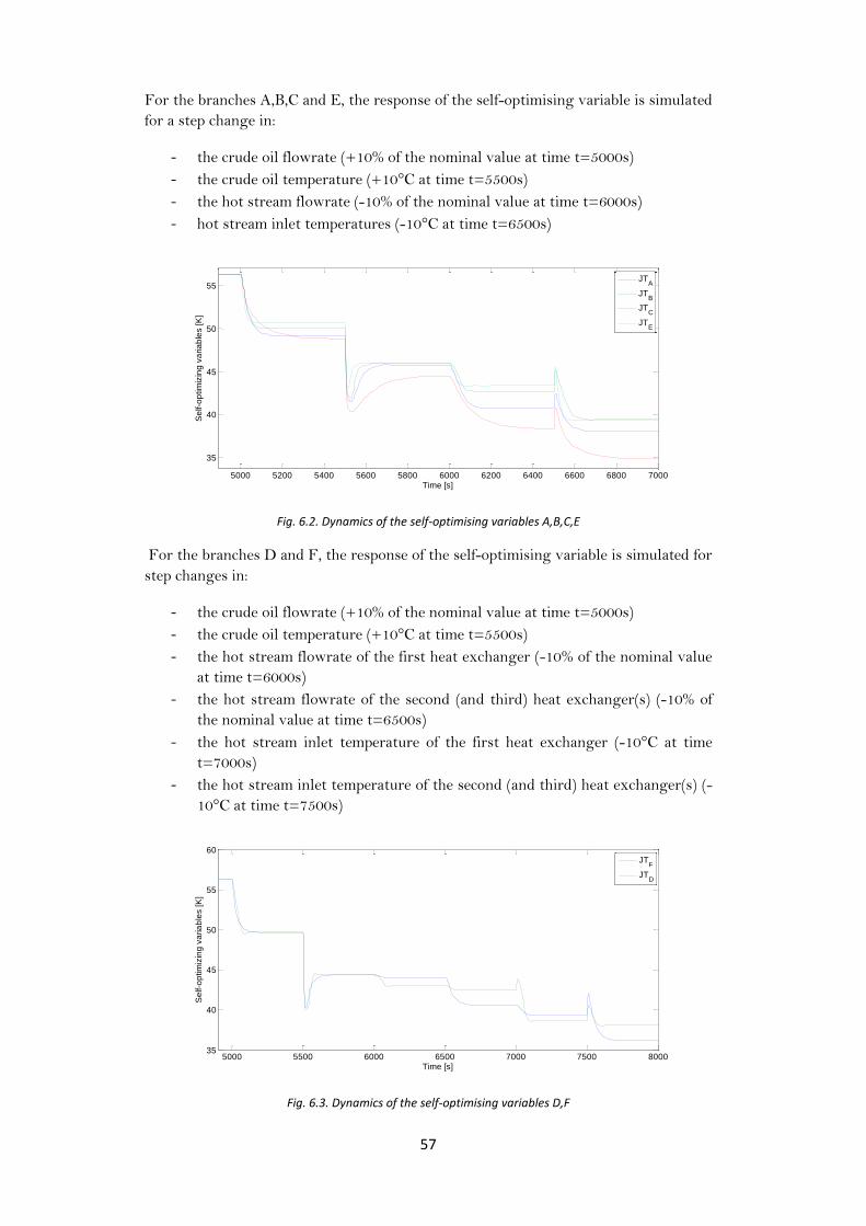
For the branches A,B,C and E, the response of the self-optimising variable is simulated
for a step change in:
- the crude oil flowrate (+10% of the nominal value at time t=5000s)
- the crude oil temperature (+10°C at time t=5500s)
- the hot stream flowrate (-10% of the nominal value at time t=6000s)
- hot stream inlet temperatures (-10°C at time t=6500s)
Fig. 6.2. Dynamics of the self-optimising variables A,B,C,E
For the branches D and F, the response of the self-optimising variable is simulated for
step changes in:
- the crude oil flowrate (+10% of the nominal value at time t=5000s)
- the crude oil temperature (+10°C at time t=5500s)
- the hot stream flowrate of the first heat exchanger (-10% of the nominal value
at time t=6000s)
- the hot stream flowrate of the second (and third) heat exchanger(s) (-10% of
the nominal value at time t=6500s)
- the hot stream inlet temperature of the first heat exchanger (-10°C at time
t=7000s)
- the hot stream inlet temperature of the second (and third) heat exchanger(s) (-
10°C at time t=7500s)
Fig. 6.3. Dynamics of the self-optimising variables D,F
5000 5200 5400 5600 5800 6000 6200 6400 6600 6800 7000
35
40
45
50
55
Time [s]
Se
lf-o
ptim
izin
g v
aria
ble
s [K
]
JTA
JTB
JTC
JTE
5000 5500 6000 6500 7000 7500 800035
40
45
50
55
60
Time [s]
Se
lf-o
ptim
izin
g v
aria
ble
s [K
]
JTF
JTD

58
The step changes in flowrates affect the self-optimising variable only by the
crude oil outlet temperature measures. The thermal capacities of the heat exchangers
thus determine the dynamics of the observed response. In this case, the self-optimising
variables present a dynamics appropriate for being used directly as controlled
variables.
For the crude oil inlet temperature step changes, direct response and
overshoots of self-optimising variable response are observed. This is due to the fact
that the self-optimising variables are function of the inlet temperature measure.
Taking the branch A as example, the numerator of the self-optimising variable is a
square function of the crude oil inlet temperature while the denominator is a linear
function. The step change affects thus very much the numerator (fast time-scale) and
this explains the overshoot. After that, the denominator stays at a constant value due
to the fact it is a function of inlet temperatures. The numerator then grows slowly
until the outlet oil temperature measure stabilises to its new higher value (slow time-
scale).
(6.1)
For the hot stream inlet temperature step changes, inverse responses are
observed. Again, this is due to the fact that denominator of the self-optimising variable
diminishes on a very fast time-scale (direct function) while the numerator diminishes
on a slow time-scale (function of the outlet temperature).
6.2. Filters for feedforward control abatement
The direct responses of the self-optimising variables are expected to be the cause of an
unwanted feedforward control by the PI controllers, even more in the case of inverse
responses. Additional dynamics on the inlet temperature measurements are thus
introduced using first-order function filters. Outlet temperature measurements
dynamics are unchanged.
6.2.1. Inlet hot temperature measurements filters
We decide to add filters for all hot stream inlet temperature measurements with such
time constant values that we reduce the impact of the inverse response of the self-
optimising variable for a -10°C step change in the hot inlet temperature to 5s.
(6.2)

59
Measured variable Filter
time constant [s]
100
240
200
160
280
40
20
240
Tab. 6.4. Filter time constants for hot inlet temperatures
Redoing the -10°C step change at time t=5000s on the inlet hot temperatures
with the filters (and at time t=6000s for the second hot stream of branches D and F),
we obtain:
Fig. 6.5. Dynamics of the self-optimising variables after hot inlet temperature filtering
6.2.2. Crude oil inlet temperature measurement filter
A step change in the crude oil inlet temperature will affect all the self-optimising
variables at the same time. Therefore, we need to consider here the dynamics of the
selected controlled variables and not the one of the self-optimising
variables .
5000 5200 5400 5600 5800 6000 6200 6400 6600 6800 700048
49
50
51
52
53
54
55
56
57
Time [s]
Se
lf-o
ptm
izin
g v
aria
ble
s m
ea
su
rem
en
ts [K
]
JTA
JTB
JTC
JTD
JTE
JTF
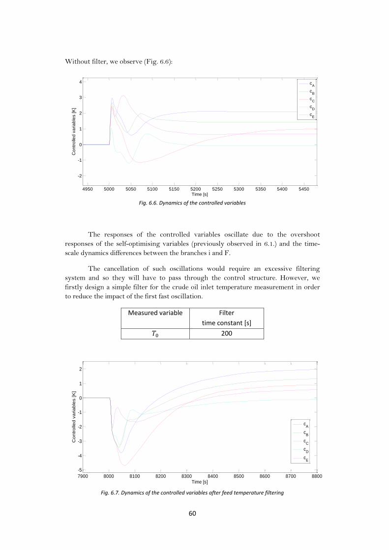
60
Without filter, we observe (Fig. 6.6):
Fig. 6.6. Dynamics of the controlled variables
The responses of the controlled variables oscillate due to the overshoot
responses of the self-optimising variables (previously observed in 6.1.) and the time-
scale dynamics differences between the branches i and F.
The cancellation of such oscillations would require an excessive filtering
system and so they will have to pass through the control structure. However, we
firstly design a simple filter for the crude oil inlet temperature measurement in order
to reduce the impact of the first fast oscillation.
Measured variable Filter
time constant [s]
200
Fig. 6.7. Dynamics of the controlled variables after feed temperature filtering
4950 5000 5050 5100 5150 5200 5250 5300 5350 5400 5450
-2
-1
0
1
2
3
4
Time [s]
Co
ntr
olle
d v
aria
ble
s [K
]
cA
cB
cC
cD
cE
7900 8000 8100 8200 8300 8400 8500 8600 8700 8800
-5
-4
-3
-2
-1
0
1
2
Time [s]
Co
ntr
olle
d v
aria
ble
s [K
]
cA
cB
cC
cD
cE

61
The impact and the fastness of the first oscillations have been very slightly
reduced (Fig.6.7.) but the improvements are very small and another kind of filter is
needed.
So, we decide to filter the self-optimising variables in order to reduce the
oscillations. Actually, we also want to avoid an extreme PI control tuning with very
short process characteristic time and very long control characteristic time that
would not lead to a smooth disturbance rejection.
Measured variable Filter
time constant [s]
30
30
10
10
100
30
The dynamics of the controlled variables is then simplified for the control
structure. On the following graph, we can observe their new response for a step
change in the crude oil inlet temperature (+10°C at time t=5000s) and the crude oil
flowrate (-10% at time t=7000s). A few oscillations remains but we now expect them
to be smoothly treated by the control structure.
Fig. 6.8. Dynamics of the controlled variables including all filters
5000 5500 6000 6500 7000 7500
-4
-3
-2
-1
0
1
2
3
4
Time [s]
Co
ntr
olle
d v
aria
ble
s [K
]
cA
cB
cC
cD
cE

62
6.3. PI controllers tuning
Each PI controller is separately tuned according to the SIMC tuning rules (cfr. section
5.5). The whole tuning process is detailed in the appendix.
Branch A B C D E
First-order
transfer function
between z and c
-237.11 -120.3 -152.17 -88.52 -137.05
[s] 64.83 58.33 61.64 48.1 99.2
[s] 12 8 10 8 10
Controller time constant
[s] 240 240 120 240 240
Controller
transfer function
-0.001085 -0.001955 -0.003116 -0.002119 -0.002895
[s] 64.83 58.33 61.64 48.1 99.2
Tab. 6.9. PI Controller tuning
6.4. Simulation results
As desired, the close-loop simulations of this first control structure made of
decentralised PI controllers and filters result in a relatively smooth operation of the
valve positions.
The following figures (Fig. 6.10 & 6.11) refer to a simulation (taken as example) made
of four successive step changes in:
- the feed temperature (+10°C at time t=5000s)
- the feed flowrate (-10% of the nominal value at time t=6000s)
- the hot stream inlet temperature on branch C (-10°C at time t=7000s)
- the hot stream flowrate on branch E (-10% at time t=8000s)
Fig.6.10. Simulation results – Outlet temperature
5000 5500 6000 6500 7000 7500 8000 8500207
208
209
210
211
212
213
214
215
216
Time [s]
Outlet
tem
pera
ture
[°C
]

63
Fig.6.11. Simulation results – Valve operation
The system especially handles very well disturbances on the hot stream
temperatures and flowrates due to the forced regular response of the controlled
variables made by the filters.
The disturbances on the feed induces conflicting dynamics responses between
each branch relative self-optimising variables as we expected from the open-loop
simulation (Fig. 6.8.) even of filters were used. This explains some fast oscillations of
the valve positions, especially on the branch E where the obtained close-loop dynamics
is in a similar same time-scale than the branch F dynamics used by the controller. (Fig.
6.11)
5000 5500 6000 6500 7000 7500 8000 8500
0.35
0.4
0.45
0.5
0.55
Time [s]
Va
lve
po
sitio
ns
zA
zB
zC
zE

64
In case of a major disturbance, the decentralised control structure is seen as a
very robust one. The new optimum point is slowly reached by the system by a smooth
operation of the valves even if the condition of one valve fully open changes from a
branch to another.
The following figures (Fig. 6.12 & 6.13) are obtained in the case of a major
step change in the second hot stream flowrate in branch F (-80% of the nominal value).
Fig.6.12. Major step change – Outlet temperature
Fig.6.13. Major step change – Valve operation
When the condition of having a valve fully open changes from the branch F to
another, the valves dynamics are slowing down. Actually, referring to the equations
(5.22) and (5.23),
(5.22)
(5.23)
When such a major change happens, the values given by each controller
have a lower impact on the system since they are treated proportionally to
which has become higher than 1. This explains the observed slow answer and so the
robustness of the control configuration for such major changes.
5000 5200 5400 5600 5800 6000 6200 6400 6600 6800 7000196
198
200
202
204
206
208
Time [s]
Ou
tle
t te
mp
era
ture
[°C
]
5000 5200 5400 5600 5800 6000 6200 6400 6600 6800 7000
0.4
0.5
0.6
0.7
0.8
0.9
1
Time [s]
Va
lve
po
sitio
ns
zA
zB
zC
zD
zE
zF
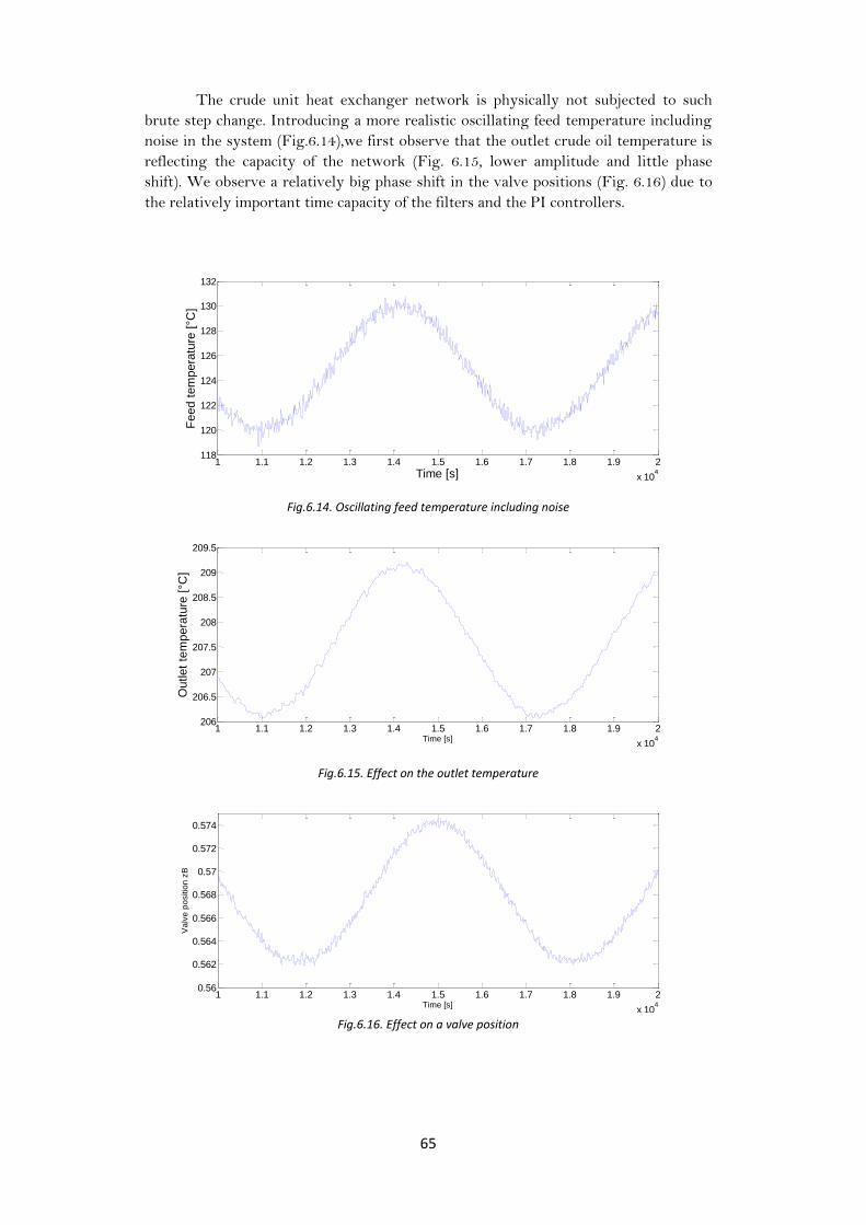
65
The crude unit heat exchanger network is physically not subjected to such
brute step change. Introducing a more realistic oscillating feed temperature including
noise in the system (Fig.6.14),we first observe that the outlet crude oil temperature is
reflecting the capacity of the network (Fig. 6.15, lower amplitude and little phase
shift). We observe a relatively big phase shift in the valve positions (Fig. 6.16) due to
the relatively important time capacity of the filters and the PI controllers.
Fig.6.14. Oscillating feed temperature including noise
Fig.6.15. Effect on the outlet temperature
Fig.6.16. Effect on a valve position
1 1.1 1.2 1.3 1.4 1.5 1.6 1.7 1.8 1.9 2
x 104
118
120
122
124
126
128
130
132
Time [s]
Feed t
em
pera
ture
[°C
]
1 1.1 1.2 1.3 1.4 1.5 1.6 1.7 1.8 1.9 2
x 104
206
206.5
207
207.5
208
208.5
209
209.5
Time [s]
Outlet
tem
pera
ture
[°C
]
1 1.1 1.2 1.3 1.4 1.5 1.6 1.7 1.8 1.9 2
x 104
0.56
0.562
0.564
0.566
0.568
0.57
0.572
0.574
Time [s]
Va
lve
po
sitio
n z
B
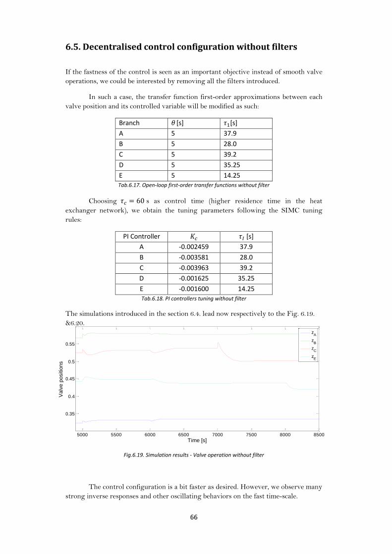
66
6.5. Decentralised control configuration without filters
If the fastness of the control is seen as an important objective instead of smooth valve
operations, we could be interested by removing all the filters introduced.
In such a case, the transfer function first-order approximations between each
valve position and its controlled variable will be modified as such:
Branch [s] [s]
A 5 37.9
B 5 28.0
C 5 39.2
D 5 35.25
E 5 14.25
Tab.6.17. Open-loop first-order transfer functions without filter
Choosing s as control time (higher residence time in the heat
exchanger network), we obtain the tuning parameters following the SIMC tuning
rules:
PI Controller [s]
A -0.002459 37.9
B -0.003581 28.0
C -0.003963 39.2
D -0.001625 35.25
E -0.001600 14.25
Tab.6.18. PI controllers tuning without filter
The simulations introduced in the section 6.4. lead now respectively to the Fig. 6.19.
&6.20.
Fig.6.19. Simulation results - Valve operation without filter
The control configuration is a bit faster as desired. However, we observe many
strong inverse responses and other oscillating behaviors on the fast time-scale.
5000 5500 6000 6500 7000 7500 8000 8500
0.35
0.4
0.45
0.5
0.55
Time [s]
Valv
e p
ositio
ns
zA
zB
zC
zE
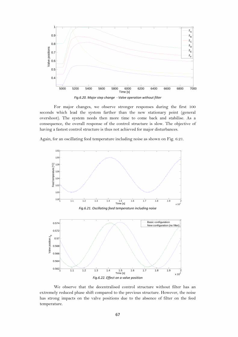
67
Fig.6.20. Major step change - Valve operation without filter
For major changes, we observe stronger responses during the first 100
seconds which lead the system farther than the new stationary point (general
overshoot). The system needs then more time to come back and stabilise. As a
consequence, the overall response of the control structure is slow. The objective of
having a fastest control structure is thus not achieved for major disturbances.
Again, for an oscillating feed temperature including noise as shown on Fig. 6.21.
Fig.6.21. Oscillating feed temperature including noise
Fig.6.22. Effect on a valve position
We observe that the decentralised control structure without filter has an
extremely reduced phase shift compared to the previous structure. However, the noise
has strong impacts on the valve positions due to the absence of filter on the feed
temperature.
1 1.1 1.2 1.3 1.4 1.5 1.6 1.7 1.8 1.9 2
x 104
118
120
122
124
126
128
130
132
Time [s]
Feed tem
pera
ture
[°C
]
1 1.1 1.2 1.3 1.4 1.5 1.6 1.7 1.8 1.9 2
x 104
0.562
0.564
0.566
0.568
0.57
0.572
0.574
Time [s]
Valv
e p
osi
tion z
B
Basic configuration
New configuration (no filter)
5000 5200 5400 5600 5800 6000 6200 6400 6600 6800 7000
0.4
0.5
0.6
0.7
0.8
0.9
1
Time [s]
Valv
e p
ositio
ns
zA
zB
zC
zD
zE
zF
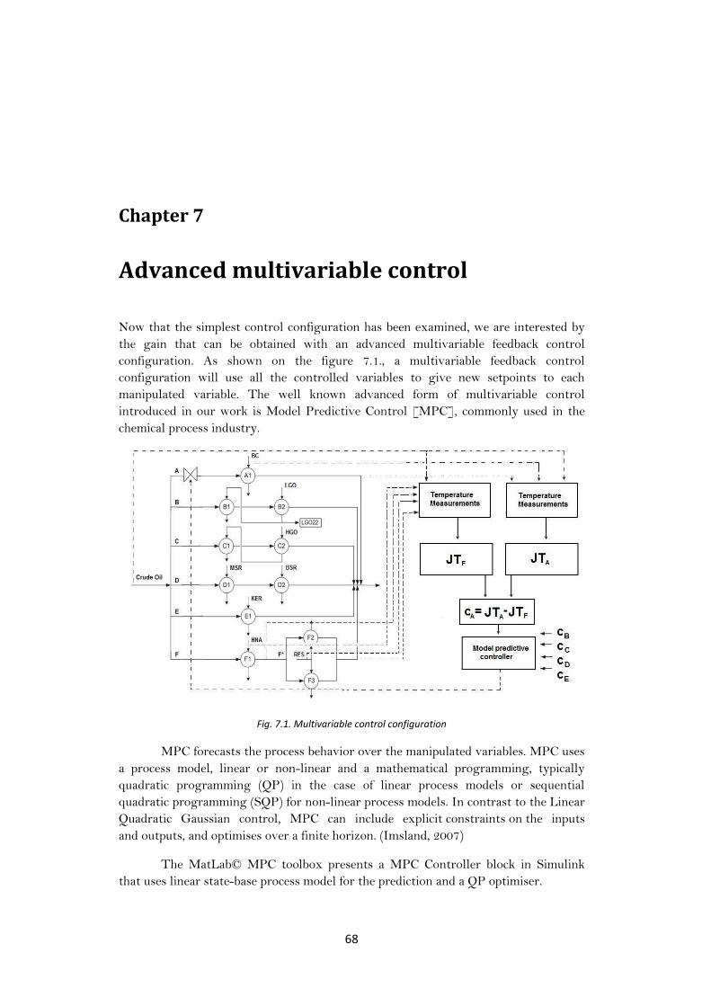
68
Chapter 7
Advanced multivariable control
Now that the simplest control configuration has been examined, we are interested by
the gain that can be obtained with an advanced multivariable feedback control
configuration. As shown on the figure 7.1., a multivariable feedback control
configuration will use all the controlled variables to give new setpoints to each
manipulated variable. The well known advanced form of multivariable control
introduced in our work is Model Predictive Control [MPC], commonly used in the
chemical process industry.
Fig. 7.1. Multivariable control configuration
MPC forecasts the process behavior over the manipulated variables. MPC uses
a process model, linear or non-linear and a mathematical programming, typically
quadratic programming (QP) in the case of linear process models or sequential
quadratic programming (SQP) for non-linear process models. In contrast to the Linear
Quadratic Gaussian control, MPC can include explicit constraints on the inputs
and outputs, and optimises over a finite horizon. (Imsland, 2007)
The MatLab© MPC toolbox presents a MPC Controller block in Simulink
that uses linear state-base process model for the prediction and a QP optimiser.
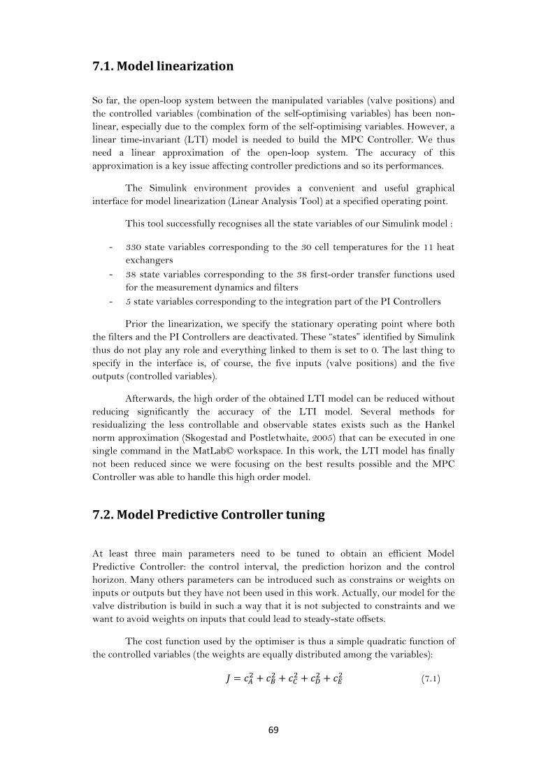
69
7.1. Model linearization
So far, the open-loop system between the manipulated variables (valve positions) and
the controlled variables (combination of the self-optimising variables) has been non-
linear, especially due to the complex form of the self-optimising variables. However, a
linear time-invariant (LTI) model is needed to build the MPC Controller. We thus
need a linear approximation of the open-loop system. The accuracy of this
approximation is a key issue affecting controller predictions and so its performances.
The Simulink environment provides a convenient and useful graphical
interface for model linearization (Linear Analysis Tool) at a specified operating point.
This tool successfully recognises all the state variables of our Simulink model :
- 330 state variables corresponding to the 30 cell temperatures for the 11 heat
exchangers
- 38 state variables corresponding to the 38 first-order transfer functions used
for the measurement dynamics and filters
- 5 state variables corresponding to the integration part of the PI Controllers
Prior the linearization, we specify the stationary operating point where both
the filters and the PI Controllers are deactivated. These “states” identified by Simulink
thus do not play any role and everything linked to them is set to 0. The last thing to
specify in the interface is, of course, the five inputs (valve positions) and the five
outputs (controlled variables).
Afterwards, the high order of the obtained LTI model can be reduced without
reducing significantly the accuracy of the LTI model. Several methods for
residualizing the less controllable and observable states exists such as the Hankel
norm approximation (Skogestad and Postletwhaite, 2005) that can be executed in one
single command in the MatLab© workspace. In this work, the LTI model has finally
not been reduced since we were focusing on the best results possible and the MPC
Controller was able to handle this high order model.
7.2. Model Predictive Controller tuning
At least three main parameters need to be tuned to obtain an efficient Model
Predictive Controller: the control interval, the prediction horizon and the control
horizon. Many others parameters can be introduced such as constrains or weights on
inputs or outputs but they have not been used in this work. Actually, our model for the
valve distribution is build in such a way that it is not subjected to constraints and we
want to avoid weights on inputs that could lead to steady-state offsets.
The cost function used by the optimiser is thus a simple quadratic function of
the controlled variables (the weights are equally distributed among the variables):
(7.1)

70
In order to have a smooth operation of the valves and reduce the impact of
inverse responses, the control interval has been set to 60 seconds which corresponds to
the highest residence time of the crude oil in the network (branch A).
The prediction horizon has to be fixed as a multiple of control intervals. Since
we focus very much on the best configuration possible, it has been set to 10 which is a
value beyond which we have not observed significant gain in the control quality of the
MPC. The control horizon has been fixed to 1 so the MPC re-optimise its prediction
and thus corrects its decision at each control interval.
7.3. Comparative simulation results
The close-loop simulation results of the MPC are shown directly in comparison with
the results of our previous decentralised control configuration using PI controllers and
filters.
As done previously, the following figures (Fig. 7.2, 7.3, 7.4) refer to a
simulation made of four successive step changes in:
- the feed temperature (+10°C at time t=5000s)
- the feed flowrate (-10% of the nominal value at time t=6000s)
- the hot stream inlet temperature on branch C (-10°C at time t=7000s)
- the hot stream flowrate on branch E (-10% at time t=8000s)
-
Fig. 7.2. Simulation results – Outlet temperature
The dynamics on the outlet temperature of the crude oil (overall objective)
does not really differ from a control configuration to another. The dynamics is mainly
a characteristic of the plant (open-loop system), the contribution of the control system
is not significant. The optimum point in the system is very flat and we know that the
valve position changes by self-optimising control only bring the same small (but
valuable) difference at the steady-state level.
5000 5500 6000 6500 7000 7500 8000 8500206
208
210
212
214
216
Time [s]
Ou
tle
t te
mp
era
ture
[°C
]
Decentralized control
MPC

71
Fig. 7.3. Simulation results – Valve operation
It appears that the valve operations are generally faster and still relatively
smooth using the MPC configuration. However, this is not observed in every
simulation and for all valve positions. All inverse responses cannot be avoided by the
MPC since we have not introduced the filters for this control configuration.
Fig. 7.4. Simulation results – Split fractions
Looking at the split fraction of the feed flowrate, we observe that faster
stabilization of the valve positions does not always lead to faster stabilization of its
branch relative crude oil flowrate due to the influence of other valve positions. As a
central controller, the MPC tends to force the branches to react in same time-scale
dynamics.
0 5000 10000 15000
0.35
0.4
0.45
0.5
0.55
Time [s]
Valv
e p
ositio
ns A
,B,C
,E
Decentralized control
MPC
5000 5500 6000 6500 7000 7500 8000 85000.11
0.115
0.12
0.125
0.13
0.135
0.14
0.145
0.15
0.155
0.16
Time [s]
Split
fractions E
,C,B
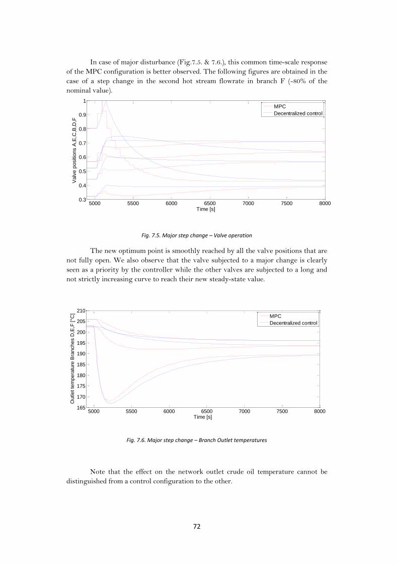
72
In case of major disturbance (Fig.7.5. & 7.6.), this common time-scale response
of the MPC configuration is better observed. The following figures are obtained in the
case of a step change in the second hot stream flowrate in branch F (-80% of the
nominal value).
Fig. 7.5. Major step change – Valve operation
The new optimum point is smoothly reached by all the valve positions that are
not fully open. We also observe that the valve subjected to a major change is clearly
seen as a priority by the controller while the other valves are subjected to a long and
not strictly increasing curve to reach their new steady-state value.
Fig. 7.6. Major step change – Branch Outlet temperatures
Note that the effect on the network outlet crude oil temperature cannot be
distinguished from a control configuration to the other.
5000 5500 6000 6500 7000 7500 80000.3
0.4
0.5
0.6
0.7
0.8
0.9
1
Time [s]
Valv
e p
ositio
ns A
,E,C
,B,D
,F
MPC
Decentralized control
5000 5500 6000 6500 7000 7500 8000165
170
175
180
185
190
195
200
205
210
Time [s]
Outlet te
mpera
ture
Bra
nches D
,E,F
[°C
]
MPC
Decentralized control

73
Fig. 7.7. Effect of an oscillating feed temperature on a valve position
For an oscillating feed temperature including noise, the MPC configuration
does not present a significant phase shift compared to a decentralised control
configuration including filters. (Fig. 7.7.) However, the noise affects much the valve
operation. The MPC simulation results would be very close to a decentralised control
configuration without filters (not shown on the graph).
1 1.1 1.2 1.3 1.4 1.5 1.6 1.7 1.8 1.9 2
x 104
0.56
0.562
0.564
0.566
0.568
0.57
0.572
0.574
Time [s]
Va
lve
po
sitio
n B
MPC
Decentralized control
74
Chapter 8
The case of flow control
8.1. Introduction
This chapter has been added here based on discussions with our industrial partner
(Statoil) in the last days of this work. It appears that flow control is actually
implemented for the operation of the given network. The control structure is then
asked to give setpoints to the crude oil flowrates of the branches A,B,C,D,E while the
crude oil flowrate of branch F results from the mass balance. Moreover, the sub-split
on branch F is given as constant.
Introducing the crude oil flowrates of the branches A,B,C,D and E as our new
manipulated variables, we decided to adapt our three previous control structure:
decentralised control with filters, decentralised control without filters and advanced
multivariable control (MPC). This chapter aims at comparing them directly and so the
explanations about the tuning will not be detailed as previously.
The objective of smooth operations is still valid in the case of flow control and
so the interest in the decentralised control structure with filters is justified. Since the
filters were introduced looking at the self-optimising variables responses for
disturbances, new manipulated variables do not lead to modifications regarding their
placement and their time constants.
8.2. Controllers re-tuning
8.2.1. Decentralised control with filters
The 5 PI controllers are retuned using the SIMC tuning rules (cfr. 5.5) (Tab. 8.1).

75
Branch A B C D E
First-order
transfer function
between z and c
-4.5573 -2.7774 -3.3026 -2.3229 -2.9914
[s] 68.9 58.2 67.9 50.4 87.0
[s] 8 9 6 8 10
Controller time constant
[s] 240 240 120 240 240
Controller
transfer function
-0.0610 -0.0842 0.1632 -0.0875 -0.1163
[s] 68.9 58.2 67.9 50.4 87.0
Tab. 8.1. PI Controllers retuning –flow decentralised control with filters
8.2.2. Decentralised control without filters
The 5 PI controllers are retuned using the SIMC tuning rules (cfr. 5.5) (Tab. 8.2).
Branch A B C D E
First-order
transfer function
between z and c
-4.5573 -2.7774 -3.3026 -2.3229 -2.9914
[s] 37.0 29.1 46.0 34.4 16.2
[s] 5 5 5 5 5
Controller time constant
[s] 60 60 60 60 60
Controller
transfer function
-0.1249 -0.1612 -0.2143 -0.2278 -0.0833
[s] 37.0 29.1 46.0 34.4 16.2
Tab. 8.2. PI Controllers retuning – flow decentralised control without filters
8.2.3. Advanced multivariable control (MPC)
For the MPC, while new manipulated variables require a new linearization, the same
tuning parameters (control interval, prediction horizon and control horizons) have
been selected.
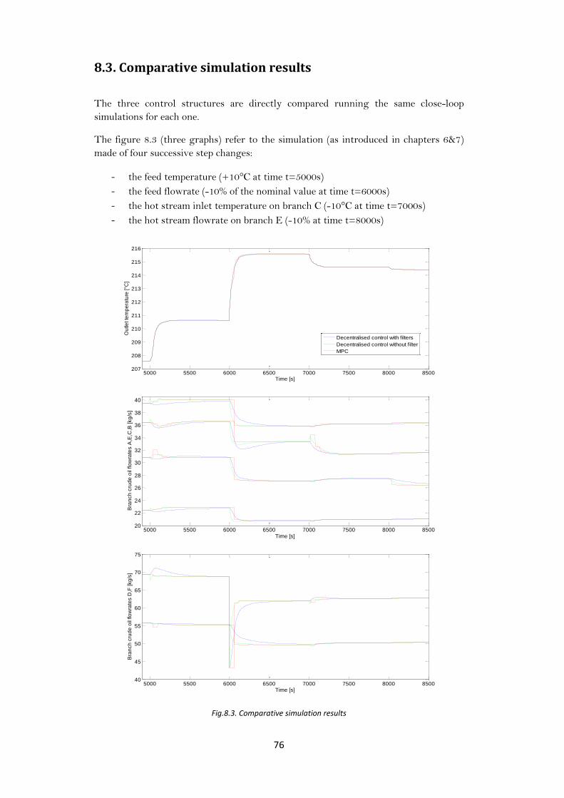
76
8.3. Comparative simulation results
The three control structures are directly compared running the same close-loop
simulations for each one.
The figure 8.3 (three graphs) refer to the simulation (as introduced in chapters 6&7)
made of four successive step changes:
- the feed temperature (+10°C at time t=5000s)
- the feed flowrate (-10% of the nominal value at time t=6000s)
- the hot stream inlet temperature on branch C (-10°C at time t=7000s)
- the hot stream flowrate on branch E (-10% at time t=8000s)
Fig.8.3. Comparative simulation results
5000 5500 6000 6500 7000 7500 8000 8500207
208
209
210
211
212
213
214
215
216
Time [s]
Ou
tlet te
mp
era
ture
[°C
]
Decentralised control with filters
Decentralised control without filter
MPC
5000 5500 6000 6500 7000 7500 8000 850020
22
24
26
28
30
32
34
36
38
40
Time [s]
Bra
nch
cru
de
oil
flo
wra
tes A
,E,C
,B [kg
/s]
5000 5500 6000 6500 7000 7500 8000 850040
45
50
55
60
65
70
75
Time [s]
Bra
nch
cru
de
oil
flow
rate
s D
,F [kg
/s]
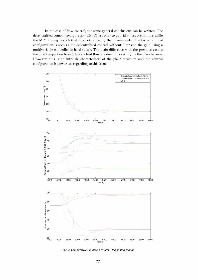
77
In the case of flow control, the same general conclusions can be written. The
decentralised control configuration with filters offer to get rid of fast oscillations while
the MPC tuning is such that it is not canceling them completely. The fastest control
configuration is seen as the decentralised control without filter and the gain using a
multivariable controller is hard to see. The main difference with the previous case is
the direct impact on branch F for a feed flowrate due to its setting by the mass balance.
However, this is an intrinsic characteristic of the plant structure and the control
configuration is powerless regarding to this issue.
Fig.8.4. Comparative simulation results – Major step change
4900 5000 5100 5200 5300 5400 5500 5600 5700 5800 5900 6000196
198
200
202
204
206
208
Time [s]
Ou
tle
t te
mp
era
ture
[°C
]
Decentralised control with filters
Decentralised control without filter
MPC
4900 5000 5100 5200 5300 5400 5500 5600 5700 5800 5900 600020
25
30
35
40
45
50
Time [s]
Bra
nch C
rude o
il flow
rate
A,E
,C,B
[kg/s
]
4900 5000 5100 5200 5300 5400 5500 5600 5700 5800 5900 600020
30
40
50
60
70
Time [s]
Bra
nch
cru
de
oil
flo
wra
te [kg
/s]
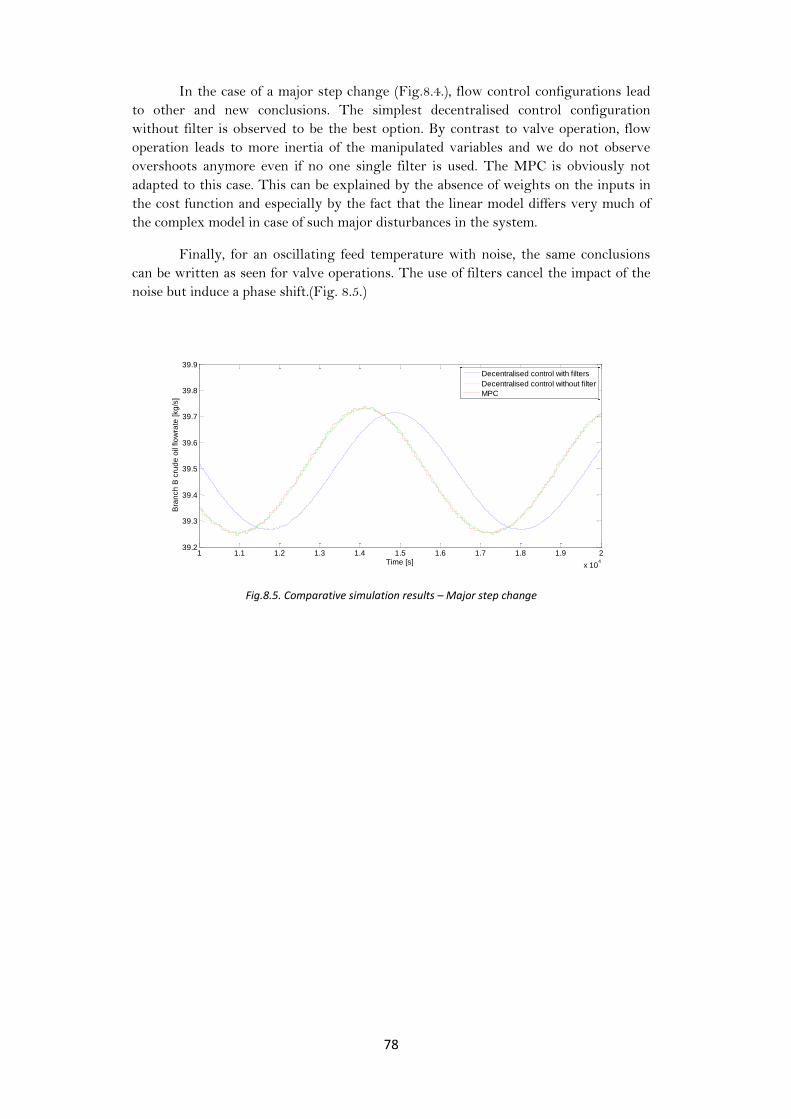
78
In the case of a major step change (Fig.8.4.), flow control configurations lead
to other and new conclusions. The simplest decentralised control configuration
without filter is observed to be the best option. By contrast to valve operation, flow
operation leads to more inertia of the manipulated variables and we do not observe
overshoots anymore even if no one single filter is used. The MPC is obviously not
adapted to this case. This can be explained by the absence of weights on the inputs in
the cost function and especially by the fact that the linear model differs very much of
the complex model in case of such major disturbances in the system.
Finally, for an oscillating feed temperature with noise, the same conclusions
can be written as seen for valve operations. The use of filters cancel the impact of the
noise but induce a phase shift.(Fig. 8.5.)
Fig.8.5. Comparative simulation results – Major step change
1 1.1 1.2 1.3 1.4 1.5 1.6 1.7 1.8 1.9 2
x 104
39.2
39.3
39.4
39.5
39.6
39.7
39.8
39.9
Time [s]
Bra
nch
B c
rud
e o
il flo
wra
te [kg
/s]
Decentralised control with filters
Decentralised control without filter
MPC
79
Chapter 9
Conclusion
The reduced crude unit heat exchanger network studied in this work presents dynamic
differences between branches that have been successfully captured in our model. Our
control design studies have thus been based on the knowledge of these physical
characteristics of the given plant.
The simple self-optimising variables derived by Jäschke (Jäschke, 2012)
present moderate steady-state performances which need to be re-assessed with an
accurate steady-state model (the values in section 4.3.2. should be considered with
caution). Nevertheless, these variables still offer to lead the system close to the optimal
point only with a few temperature measurements.
The self-optimising variables dynamics present undesirable transient effects,
especially at high frequencies (fast-time scales). Since the control pursues an
economical objective, smooth operation has been sought in this work. So filtering on
selective measurements (feedforward control abatement, etc.) has been suggested to
limit any hard valve or flow operation in the case of a simple control configuration.
A decentralised control configuration made of 5 simple PI controllers is
believed to be satisfactory for the operation of the given network. In this case, the
operation smoothness is balanced with the control phase shift due to the filters. The
close-loop system is observed to have a strong robustness and so can handle safely
huge disturbances. This control configuration will not require any modeling effort for
industrial implementation which constitutes a major advantage.
The overall results of the MPC configuration are considered to be only a bit
better than those of the decentralised control configuration using filters. Actually, the
MPC computes a close-loop optimal time-scale dynamics which can be approximately
found in the decentralised configuration (tuning of each PI controllers separately). If
relatively hard valve or flow operations were allowed, there would not be significant
differences between the dynamics performances of a decentralised control
configuration without filters and the MPC configuration.
However, the physical computing time of the MPC has not been taken into
account and could lead to a poorer performance on the real plant compared to fast PI
controllers.
A.Leruth, June 2012

80
Bibliography
Boyaci, C., Uzturk, D., Konukman, A. E. S., Akman, U., 1996. Dynamics and Optimal
Control of Flexible Heat-Exchanger Networks. Computers and Chemical Engineering
20 (Supplement 2), 775 – 780.
Chachuat, B., Srinivasan, B., Bonvin, D., 2009. Adaptation Strategies for Real-Time
Optimisation. Computers and Chemical Engineering 33 (10), 1557 – 1567.
Edvardsen, D.G., 2011, Optimal operation of Heat Exchanger Networks, master
thesis, Norwegian University of Science and Technology.
Glemmestad, B., Skogestad, S., Gundersen, T., 1999. Optimal operation of heat
exchanger networks. Computers and Chemical Engineering 23 (4-5), 509 – 522.
I.A. Wiehe and R.J.Kennedy, 2000, Energy and Fuels, 14, 56-63
Imsland L., 2007, An introduction to Model Predictive Control, Norwegian University
of Science and Technology
Jäschke, J., 2011. Invariants for Optimal Operation of Process Systems. Doctoral
thesis, Norwegian University of Science and Technology.
Jäschke J., 2012, United Kingdom Patent Application No. 1207770.7, Parallel Heat
Exchanger control
Lid,T.,Strand,S.,Skogestad,S.,On-line optimisation of a crude unit heat exchanger
network, 2000
Lid, T., Skogestad, S., 2001. Implementation issues for real-time optimisation of a
crude unit heat exchanger network. In: Gani,R.,Jorgensen,S.B.(Eds.),European
Symposium on Computer Aided Process Engineering - 11, 34th European Symposium
of the Working Party on Computer Aided Process Engineering. Vol. 9 of Computer
Aided Chemical Engineering. Elsevier, pp. 1041 – 1046.
Lundsford K.M., 1998, Increasing heat exchanger performance, Bryan research and
Engineering, Inc. Texas
Mathisen, K. W., Skogestad, S., Wolff, E. A., 1992. Bypass Selection for Control of
Heat Exchanger Networks. Computers and Chemical Engineering 16 (Supplement 1),
263 – 272.
Mathisen, K.W., Morari, M., Skogestad, S., Wolff, E. A., 1994a. Optimal Operation of
Heat Exchanger Networks Presented at Process Systems Engineering (PSE’94),
Kyongju, Korea.
Mathisen, K. W., Morari, M., Skogestad, S., 1994b. Dynamic models for heat
exchangers and heat exchanger networks. Computers and Chemical Engineering 18
(1), 459–463.
Sinnott, R., Towler, G., 2009. Chemical Engineering Design, 5th Edition. Elsevier
Ltd., Oxford.

81
Skogestad, S., 2000. Plantwide control: the search for the self-optimising control
structure. Journal of Process Control 10.
Skogestad, S., 2003, Simple analytic rules for model reduction and PID controller
tuning, Journal of Process Control 13, 291–309
Skogestad, S., 2004, Near-optimal operation by self-optimizing control: From process
control to marathon running and business systems, Computers & Chemical
Engineering 29(1), 127-137
Skogestad, S., Postelthwaite, I., 2005, Multivariable feedback control, Analysis and
Design, John Wiley & Sons, Ltd, Second edition
White, D. C., 1997. Online optimisation: What, where and estimating ROI. Hydro-
carbon Processing 76 (6), 4351.
Web resources:
http://www.mathworks.se/help/toolbox/simulink/
http://www.alaquainc.com/Heat_Exchangers.aspx
http://www.substech.com/dokuwiki/doku.php?id=stainless_steel_2205
http://synergycoils.com/products/tube/index.htm

82
Appendix
A. Data Reconciliation – Temperatures and flowrates
Branch A :
Since was missing in the asked data, this heat balance just serves to compute it.
All others measured data are taken without any modification.
76,582 125,00 226,457 295,4453 167,59
Branch B :
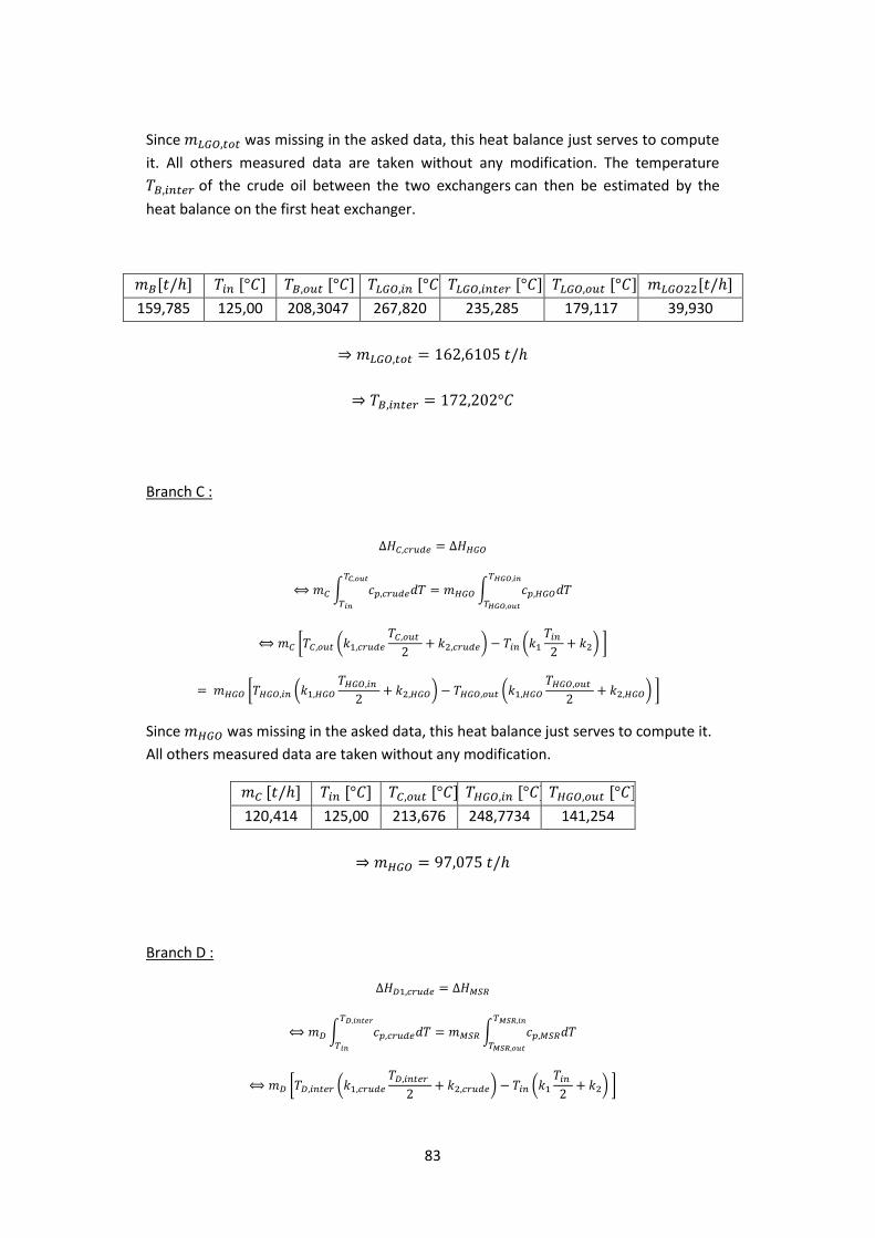
83
Since was missing in the asked data, this heat balance just serves to compute
it. All others measured data are taken without any modification. The temperature
of the crude oil between the two exchangers can then be estimated by the
heat balance on the first heat exchanger.
159,785 125,00 208,3047 267,820 235,285 179,117 39,930
Branch C :
Since was missing in the asked data, this heat balance just serves to compute it.
All others measured data are taken without any modification.
120,414 125,00 213,676 248,7734 141,254
Branch D :
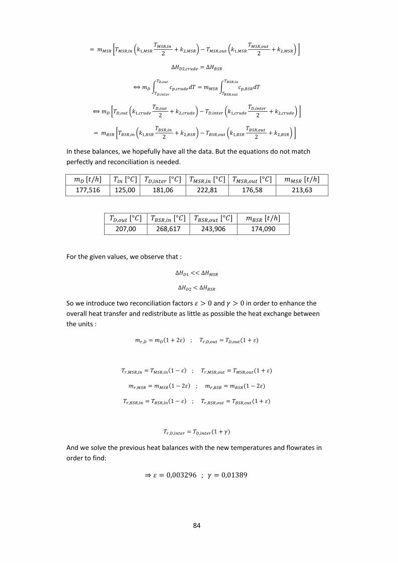
84
In these balances, we hopefully have all the data. But the equations do not match
perfectly and reconciliation is needed.
177,516 125,00 181,06 222,81 176,58 213,63
207,00 268,617 243,906 174,090
For the given values, we observe that :
So we introduce two reconciliation factors and in order to enhance the
overall heat transfer and redistribute as little as possible the heat exchange between
the units :
And we solve the previous heat balances with the new temperatures and flowrates in
order to find:
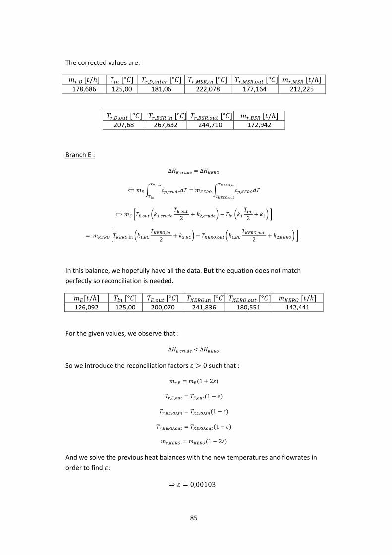
85
The corrected values are:
178,686 125,00 181,06 222,078 177,164 212,225
207,68 267,632 244,710 172,942
Branch E :
In this balance, we hopefully have all the data. But the equation does not match
perfectly so reconciliation is needed.
126,092 125,00 200,070 241,836 180,551 142,441
For the given values, we observe that :
So we introduce the reconciliation factors such that :
And we solve the previous heat balances with the new temperatures and flowrates in
order to find :

86
The corrected values are:
126,351 125,00 200,276 241,587 180,7366 142,1482
Branch F : cfr. report.
Global balances on the crude oil :
Mass balance :
Since was not part of the asked data, this mass balance is used to estimate it.
Heat balance (cfr. 2.3.1. (*)) :
In order to simplify the reconciliation procedure, is calculated by this expression.
For information, the measured was 206,6836°C. The reconciliation forces it to a
0,47% adjustment.

87
B. PI controllers tuning (valve control with filters)
Open-loop step change in the valve position of branch E
At time t=5000s, passes from 0.4428 to 0.4528
The step response is used to approximate a first order transfer function between the
manipulated variable and the controlled variable including time delay:
With:
According to the SIMC tuning rules and choosing
With :
5000 5100 5200 5300 5400 5500 5600
-1.5
-1
-0.5
0
0.5
Time [s]
Co
ntr
olle
d v
aria
ble
[K
]
CV
First order approximation

88
Open-loop step change in the valve position of branch A
At time t=8000s, passes from 0.3220 to 0.3320
The step response is used to approximate a first order transfer function between the
manipulated variable and the controlled variable including time delay:
With:
According to the SIMC tuning rules and choosing
With :
8000 8050 8100 8150 8200 8250 8300 8350 8400
-2
-1.5
-1
-0.5
0
Time [s]
Co
ntr
olle
d v
aria
ble
[K
]
CV
First order approximation

89
Open-loop step change in the valve position of branch B
At time t=8000s, passes from 0.5680 to 0.5780
The step response is used to approximate a first order transfer function between the
manipulated variable and the controlled variable including time delay:
With:
According to the SIMC tuning rules and choosing
With :
8000 8050 8100 8150 8200 8250 8300 8350 8400
-1.2
-1
-0.8
-0.6
-0.4
-0.2
0
Time [s]
Co
ntr
olle
d v
aria
ble
[K
]
CV
First order approximation
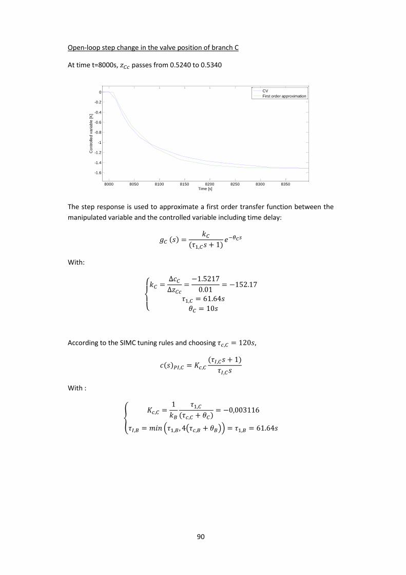
90
Open-loop step change in the valve position of branch C
At time t=8000s, passes from 0.5240 to 0.5340
The step response is used to approximate a first order transfer function between the
manipulated variable and the controlled variable including time delay:
With:
According to the SIMC tuning rules and choosing
With :
8000 8050 8100 8150 8200 8250 8300 8350
-1.6
-1.4
-1.2
-1
-0.8
-0.6
-0.4
-0.2
0
Time [s]
Co
ntr
olle
d v
aria
ble
[K
]
CV
First order approximation
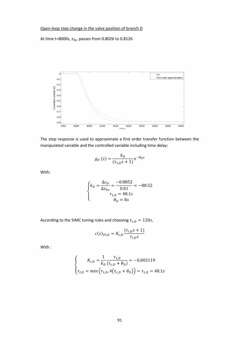
91
Open-loop step change in the valve position of branch D
At time t=8000s, passes from 0.8026 to 0.8126
The step response is used to approximate a first order transfer function between the
manipulated variable and the controlled variable including time delay:
With:
According to the SIMC tuning rules and choosing
With :
7950 8000 8050 8100 8150 8200 8250 8300 8350 8400
-0.9
-0.8
-0.7
-0.6
-0.5
-0.4
-0.3
-0.2
-0.1
0
Time [s]
Co
ntr
olle
d v
aria
ble
[K
]
CV
First order approximation

92
C. MatLab© code
Main file – run.m
%% Load initial values
initial;
%% Choice of the control type and configuration
Case=1; %0:valve control, 1:flow control
PIControl=1; %0:off, 1:on
MPControl=0; %0:off, 1:on
Filters=0; %0:off, 1:on
if MPControl ==1 %avoid errors, MPC not to be used with PIs or filters
Filters=0;
PIControl=0;
end
%Activation time for controllers
tPIControl=2000;
tMPControl=2000;
%% Controllers tuning
if Case==0
load('MPC6010.mat'); %MPC
if Filters==1 % PIs
SIMCtuning;
else
SIMCtuningnf;
end
else
load('MPC6010flow.mat');
if Filters==1;
SIMCtuningflow;
else
SIMCtuningflownf;
end
end
%% Filters time constants [seconds]
tm=5; %temperature sensor time constant
if Filters==1
taT0=200;
taF1in=20;
taF2in=240;
taEin=40;
taAin=100;
taBin=240;
taCin=200;
taD1in=160;
taD2in=320;
tfF=30;
tfA=30;
tfB=30;
tfC=10;
tfD=10;
tfE=100;
else
taT0=0;
taF1in=0;
taF2in=0;
taEin=0;
taAin=0;
taBin=0;
taCin=0;
taD1in=0;
taD2in=0;
tfF=0;
tfA=0;
tfB=0;
tfC=0;
tfD=0;
tfE=0;
end

93
%% Initial values for Self-optimising control
%Overwriting of the Mongstad initial values
if PIControl+MPControl == 1
zAin=0.321952537153837;
zBin=0.567990778724905;
zCin=0.523955679372974;
zDin=0.802799870251506;
zEin=0.442765317157139;
zin=[zAin zBin zCin zDin zEin];
ztotin=zAin+zBin+zCin+zDin+zEin+zFin;
mAin=0.088007924682618*m0;
mBin=0.155273650881162*m0;
mCin=0.143229693127898*m0;
mDin=0.219459994392951*m0;
mEin=0.121049941148732*m0;
end
%% Run Simulink
if Case == 0
sim('Valvecontrol') %Simulink file for valve control
else
sim('Flowcontrol') % Simulink file for flow control
end
initial.m %%
%Load initial values, 23-10-2011 18h10 36''+reconciliation
%CRUDE OIL FEED
T0=125; %°C
m0A=76.582/3.6; %t/h -> kg/s
m0B=159.785/3.6;
m0C=120.414/3.6;
m0D=178.686/3.6;
m0E=126.351/3.6;
m0F=253.604/3.6;
m0=m0A+m0B+m0C+m0D+m0E+m0F;
%Heat capacities
capacities;
%Branch A
uAin=m0A/m0; %split fraction []
ThinA=295.4453; %Hot stream inlet temperature [°C]
cp_hA=k1A*ThinA+k2A; %Hot stream inlet heat capacity [J/kgK]
mhA=57.270/3.6; %Hot stream flowrate [kg/s]
%Branch B
uBin=m0B/m0;
ThinB=267.82;
cp_hB=k1B*ThinB+k2B;
mhB=162.6105/3.6;
LGO22=39.92969/3.6;
%Branch C
uCin=m0C/m0;
ThinC=248.7734;
cp_hC=k1C*ThinC+k2C;
mhC=97.075/3.6;
% Branch D
uDin=m0D/m0;
ThinD1=222.078;
cp_hD1 =k1D1*ThinD1+k2D1;
mhD1=212.225/3.6;

94
ThinD2=267.632;
cp_hD2=k1D2*ThinD2+k2D2;
mhD2=172.942/3.6;
%Branch E
uEin=m0E/m0;
ThinE=241.587;
cp_hE=k1E*ThinE+k2E;
mhE=142.1482/3.6;
% Branch F
ThinF1=193.843;
cp_hF1=k1F1*ThinF1+k2F1;
mhF1=72.125/3.6;
ThinF2=244.379;
cp_hF2=k1F2*ThinF2+k2F2;
mhF2=(113.081+110.689)/3.6;
% Branch F - Sub-branches F2-F3
splith=110.689/(113.081+110.689); %Hot split fraction
splitc=119.91/253.604; %Cold split fraction
%%
%Initial valve positions computations
z0=[0.8 0.8 0.8 0.8 0.8];
uin=[uAin uBin uCin uDin uEin]; %We know the split fractions
zFin=1; %Olavalve - the valve position on the main branch (F) is fixed to 1
options = optimset('TolFun',1e-15);
z=fsolve(@(z) vav(z,uin,zFin),z0,options); %solver
zin=[z zFin]; %intial valve positions (result)
zF3in=1;
zF2in=(splitc/(1-splitc))*zF3in;
%%
%Initial values given to the filters
zeros = [0 0 0 0 0];
in3A=[125 295.4453 226.4550761762809];
in3B=[125 267.82 208.2976010282482];
in3C=[125 248.7734 213.6725976653782];
in5D=[125 222.078 267.632 181.0689995365419 207.6791409932723];
in3E=[125 241.587 200.2790677090032];
in5F=[125 193.843 244.379 137.5308748959151 202.2179313771867];
in3F2=[137.5308748959151 244.379 205.7564625690082];
in3F3=[137.5308748959151 244.379 199.0270239621444];
vav.m function res=vav(z,uin,zFin)
for i=1:5
res(i)=uin(i)-(z(i)/(sum(z)+zFin));
end
end
capacities.m %capacities constants: cp=k1T+k2 [J/kgK]
%Crude oil
k1=1000*(2.0*2.1297e-003);
k2=1000*1.7895;
%Hot streams
k1A=1000*(2.0*1.9783e-003); %BC
k2A=1000*1.7771; %BC

95
k1B=1000*(2.0*2.0636e-003); %LGO
k2B=1000*1.7963; %LGO
k1C=1000*(2.0*1.9901e-003); %HGO
k2C=1000*1.7924; %HGO
k1D1=1000*(2.0*2.2292e-003); %MSR
k2D1=1000*1.7967; %MSR
k1D2=1000*(2.0*2.0483e-003); %BSR
k2D2=1000*1.7877; %BSR
k1E=1000*(2.0*2.2148e-003); %KERO
k2E=1000*1.7941; %KERO
k1F1=1000*(2.0*2.4663e-003); %HNA
k2F1=1000*1.7791; %HNA
k1F2=1000*(2.0*1.8189e-003); %RES
k2F2=1000*1.7798; %RES
SIMCtuning.m %Branch E
kE=-137.05;
tetaE=10;
tau1E=109.2-tetaE;
taucE=240;
KcE=tau1E/(kE*(taucE+tetaE));
tauiE=tau1E;
%Branch A
kA=-237.11;
tetaA=12;
tau1A=76.83-tetaA;
taucA=240;
KcA=tau1A/(kA*(taucA+tetaA));
tauiA=tau1A;
%Branch B
kB=-120.3;
tetaB=8;
tau1B=66.33-tetaB;
taucB=240;
KcB=tau1B/(kB*(taucB+tetaB));
tauiB=tau1B;
%Branch C
kC=-152.17;
tetaC=10;
tau1C=71.64-tetaC;
taucC=120;
KcC=tau1C/(kC*(taucC+tetaC));
tauiC=tau1C;
%Branch D
kD=-88.52;
tetaD=8;
tau1D=56.1-tetaD;
taucD=240;
KcD=tau1D/(kD*(taucD+tetaD));
tauiD=tau1D;

96
SIMCtuningnf.m
%Branch E
kE=-137.05;
tetaE=5;
tau1E=19.25-tetaE;
taucE=60;
KcE=tau1E/(kE*(taucE+tetaE));
tauiE=tau1E;
%Branch A
kA=-237.11;
tetaA=5;
tau1A=42.9-tetaA;
taucA=60;
KcA=tau1A/(kA*(taucA+tetaA));
tauiA=tau1A;
%Branch B
kB=-120.3;
tetaB=5;
tau1B=33-tetaB;
taucB=60;
KcB=tau1B/(kB*(taucB+tetaB));
tauiB=tau1B;
%Branch C
kC=-152.17;
tetaC=5;
tau1C=44.2-tetaC;
taucC=60;
KcC=tau1C/(kC*(taucC+tetaC));
tauiC=tau1C;
%Branch D
kD=-88.52;
tetaD=5;
tau1D=40.25-tetaD;
taucD=240;
KcD=tau1D/(kD*(taucD+tetaD));
tauiD=tau1D;
SIMCtuningflow.m %Branch E
kE=-2.9914;
tetaE=10;
tau1E=97-tetaE;
taucE=240;
KcE=tau1E/(kE*(taucE+tetaE));
tauiE=tau1E;
%Branch A
kA=-4.5573;
tetaA=8;
tau1A=76.9-tetaA;
taucA=240;
KcA=tau1A/(kA*(taucA+tetaA));
tauiA=tau1A;
%Branch B
kB=-2.7774;
tetaB=9;
tau1B=67.2-tetaB;
taucB=240;
KcB=tau1B/(kB*(taucB+tetaB));
tauiB=tau1B;

97
%Branch C
kC=-3.3026;
tetaC=6;
tau1C=73.9-tetaC;
taucC=120;
KcC=tau1C/(kC*(taucC+tetaC));
tauiC=tau1C;
%Branch D
kD=-2.3229;
tetaD=8;
tau1D=58.4-tetaD;
taucD=240;
KcD=tau1D/(kD*(taucD+tetaD));
tauiD=tau1D;
SIMCtuningflownf.m
%Branch E
kE=-137.05;
tetaE=5;
tau1E=19.25-tetaE;
taucE=60;
KcE=tau1E/(kE*(taucE+tetaE));
tauiE=tau1E;
%Branch A
kA=-237.11;
tetaA=5;
tau1A=42.9-tetaA;
taucA=60;
KcA=tau1A/(kA*(taucA+tetaA));
tauiA=tau1A;
%Branch B
kB=-120.3;
tetaB=5;
tau1B=33-tetaB;
taucB=60;
KcB=tau1B/(kB*(taucB+tetaB));
tauiB=tau1B;
%Branch C
kC=-152.17;
tetaC=5;
tau1C=44.2-tetaC;
taucC=60;
KcC=tau1C/(kC*(taucC+tetaC));
tauiC=tau1C;
%Branch D
kD=-88.52;
tetaD=5;
tau1D=40.25-tetaD;
taucD=240;
KcD=tau1D/(kD*(taucD+tetaD));
tauiD=tau1D;

98
Heat exchanger model – s-function
Heat exchanger S-function m-file
[hexchXX.m] Indexch
[Y] A hexch3.m 4
B1 hexch41.m 5 B2 hexch42.m 6 C1 hexch51.m 7 C2 hexch52.m 8 D1 hexch61.m 9 D2 hexch62.m 10 E hexch2.m 3
F1 hexch11.m 1 F2 hexch12.m 2 F3 hexch13.m 11
hexchXX.m
function [sys,x0] = hexchXX(t,x,u,flag)
Indexch=Y; N = 10;
%
% Simulink interface, exchanger consisting of three series of lump systems :
% Hot side, Wall, Cold side
%
% t - time in [s].
% X - State, the first N states are hot temperatures,
% the second N states are wall temperatures,
% the last N states are cold temperatures.
% Inputs:
% U(1) - Inlet hot temperature
% U(2) - Inlet hot mass flow
% U(3) - Inlet cold temperature
% U(4) - Inlet cold mass flow
% Outputs: When flag is 0 sys contains sizes and x0 contains initial condition.
% When flag is 1, sys contains the state derivatives.
% When flag is 3 sys contains outputs;
% y(1) - Oulet hot temperature
% y(2) - Oulet hot mass flow
% y(3) - Outlet cold temperature
% y(4) - Outlet cold mass flow
if abs(flag) == 1 % Return state derivatives.
sys = mathisen(t,x,u,N,Indexch);
elseif abs(flag) == 3 % Return system outputs.
sys(1,1) = x(N); % Outlet hot temperature
sys(2,1) = x(3*N); % Outlet cold temperature
elseif flag == 0 % Initialise the system
x0 = steadyvar(Indexch,N);
sys = [3*N,0,2,4,0,0]; %number of continuous states, discrete states, outputs,
inputs
else
sys = [];
end
end

99
mathisen.m
function xprime=mathisen(t,X,U,N,Indexch)
%Variables name substitution
Thot=X(1:N);
Twall=X(N+1:2*N);
Tcold=X(2*N+1:3*N);
Thin=U(1);
Mhin=U(2);
Tcin=U(3);
Mcin=U(4);
[Ai,Vh,Vc,V_w,rho_w,cp_w]=data(Indexch,N); %load heat exchanger data
%Computations of physical values in each fluid cell
cp_c = 1000*(2.0*2.1297e-003)*Tcold + 1000*1.7895; %CRUDE OIL
rho_c = 735.96;
if Indexch==1
cp_h = 1000*(2.0*2.4663e-003*Thot + 1.7791); %HNA
rho_h = 663.196;
h_c = 1381; %W/(m^2K)
h_h = h_c;
elseif Indexch==2 | Indexch==11
cp_h = 1000*(2.0*1.8189e-003*Thot + 1.7798); %RES
rho_h = 832.86;
if Indexch==2
h_c = 1462.5; %W/(m^2K)
h_h = h_c;
else
h_c = 1257.5; %W/(m^2K)
h_h = h_c;
end
elseif Indexch==3
cp_h = 1000*(2.0*2.2148e-003*Thot + 1.7941); %KERO
rho_h = 682.727;
h_c = 1976; %W/(m^2K)
h_h = h_c;
elseif Indexch==4
cp_h = 1000*(2.0*1.9783e-003*Thot + 1.7771); %BC
rho_h = 736.938; %BC like BSR
h_c = 1902; %W/(m^2K)
h_h = h_c;
elseif Indexch==5 |Indexch==6
cp_h = 1000*(2.0*2.0636e-003*Thot + 1.7963); %LGO
rho_h= 718.929;
if Indexch==5
h_c = 1189; %W/(m^2K)
h_h = h_c;
else
h_c = 713; %W/(m^2K)
h_h = h_c;
end
elseif Indexch==7|Indexch==8
cp_h = 1000*(2.0*1.9901e-003*Thot + 1.7924); %HGO
rho_h = 788.892;
h_c = 1565; %W/(m^2K)
h_h = h_c;
elseif Indexch==9
cp_h = 1000*(2.0*2.2292e-003*Thot + 1.7967); %MSR
rho_h= 690.296;%MPA
h_c = 1250; %W/(m^2K)
h_h = h_c;
else
cp_h = 1000*(2.0*2.0483e-003*Thot + 1.7877); %BSR
rho_h= 719.023; %BPA
h_c = 382.5; %W/(m^2K)
h_h = h_c;
end
w_h=Mhin*cp_h;
w_c=Mcin*cp_c;

100
% State equations
dThotdt(1)=(Thin-Thot(1)-((h_h*Ai)/(w_h(1)*N))*(Thot(1)-
Twall(N)))*((Mhin*N)/(rho_h*Vh));
dTwalldt(1)=(h_h*(Thot(N)-Twall(1))-h_c*(Twall(1)-
Tcold(1)))*(Ai/(rho_w*cp_w*V_w));
dTcolddt(1)=(Tcin-Tcold(1)-((h_c*Ai)/(w_c(1)*N))*(Tcold(1)-
Twall(1)))*((Mcin*N)/(rho_c*Vc));
for i=2:N
j=N-i+1;
dThotdt(i)=(Thot(i-1)-Thot(i)-((h_h*Ai)/(w_h(i)*N))*(Thot(i)-
Twall(j)))*((Mhin*N)/(rho_h*Vh));
end
for j=2:N
i=N-j+1;
dTwalldt(j)=(h_h*(Thot(i)-Twall(j))-h_c*(Twall(j)-
Tcold(j)))*(Ai/(rho_w*cp_w*V_w));
dTcolddt(j)=(Tcold(j-1)-Tcold(j)-((h_c*Ai)/(w_c(j)*N))*(Tcold(j)-
Twall(j)))*((Mcin*N)/(rho_c*Vc));
end
xprime=[dThotdt,dTwalldt,dTcolddt];
data.m
function [Ai,Vh,Vc,V_w,rho_w,cp_w]=data(Indexch,N)
%Areas data [m2]
A = [77,278,164,138,162,203,264,233,260,313,278];
Ai = A(Indexch);
%Volumes data [m3]
Vshell = [0.67,2.5,1.2,1.7,1.287,1.718,2.38,2.049,1.86,2.61,2.53];
Vbundle= [0.45,1.39,0.7,0.8,0.712,0.96,1.4,1.151,1.25,1.88,1.33];
Vcs =
[Vbundle(1),Vbundle(2),Vbundle(3),Vshell(4),Vshell(5),Vbundle(6),Vbundle(7),Vbund
le(8),Vbundle(9),Vshell(10),Vbundle(11)]; %cold side - crude oil
Vhs =
[Vshell(1),Vshell(2),Vshell(3),Vbundle(4),Vbundle(5),Vshell(6),Vshell(7),Vshell(8
),Vshell(9),Vbundle(10),Vshell(11)]; %hot side
Vc = Vcs(Indexch);
Vh = Vhs(Indexch);
% Wall = bundle
cp_w = 460; %P, Wall heat capacity [J/kg*K]
rho_w = 7800; %P, Wall density [kg/m3]
mass_w = [1580,5520,3060,3760,3080,4070,5480,4830,4910,6400,5610]; % Weight
bundle [kg]
V_w = mass_w(Indexch)/(rho_w*N); % Wall volumes [m3]
steadyvar.m
function [x0]=steadyvar(Indexch,N)
if N==10
if Indexch==1
x0 =
[188.821189347093,184.064371788945,179.563318018329,175.308633179628,171.29081248
9110,167.500294502864,163.927511482946,160.562936414220,157.397126327431,154.4207
61684806,140.172731397991,142.154641626783,144.264464582883,146.508736188978,148.
894114621792,151.427356930430,154.115292927563,156.964796452930,159.982754170073,
163.176032121504,125.924701111176,126.912156926135,127.965992751546,129.089960895
010,130.287934740721,131.563901371750,132.921952675497,134.366274887530,135.90113
6551200,137.530874895915];

101
elseif Indexch==2
x0 =
[236.645169196325,228.979210519106,221.380614583620,213.848839383696,206.38330963
3788,198.983416089576,191.648514843408,184.377926590477,177.170935861114,170.0267
90214042,157.069346005094,163.957862563544,170.904102585451,177.908794841917,184.
972632022200,192.096271600505,199.280336658768,206.525416670782,213.832068252481,
221.200815882667,144.111901796146,150.744789265973,157.430278580425,164.169074840
427,170.961847954824,177.809233567223,184.711833933841,191.670218757944,198.68492
5985856,205.756462569008];
elseif Indexch==3
x0 =
[236.373709983483,230.982947919496,225.404371406103,219.626676693288,213.63747114
0236,207.423123259489,200.968585365540,194.257182486298,187.270359391236,179.9873
75167395,156.991644174346,164.935106621032,172.549299704039,179.857723120800,186.
881362944870,193.639046937299,200.147738284952,206.422780261969,212.478101429496,
218.326388846243,133.995913181297,142.599853850828,150.841416921781,158.746860876
059,166.339602630251,173.640622734361,180.668799876615,187.441189117834,193.97325
4939495,200.279067709003];
elseif Indexch==4
x0 =
[280.105847433722,265.270155263516,250.942430745715,237.125749239346,223.82198694
6348,211.031764266429,198.754401507834,186.987888481732,175.728869220856,164.9726
42710383,149.132063850481,158.857418773925,169.038275704907,179.679070574804,190.
783037781288,202.352208176369,214.387421221824,226.888350549594,239.853541855826,
253.280461805001,133.291484990579,141.985968326993,151.088662928083,160.603739641
774,170.534311296148,180.882429406391,191.649093204303,202.834270353472,214.43692
8448136,226.455076176281];
elseif Indexch==5
x0 =
[229.238047599607,223.405389839306,217.617771012971,211.875806451550,206.18011234
3944,200.531305193487,194.930001245251,189.376815883875,183.872363001763,178.4172
54337545,153.974046795688,158.988798857398,164.049753115224,169.156353847588,174.
308042720652,179.504259408939,184.744442189478,190.028028509423,195.354455527254,
200.723160627711,129.530839253832,134.105234713033,138.722690346573,143.382706449
925,148.084780247816,152.828406473935,157.613077927406,162.438286005875,167.30352
1215201,172.208273655815];
elseif Indexch==6
x0 =
[264.692200523635,261.534750811916,258.346932040025,255.127997102887,251.87716905
9616,248.593639467202,245.276566593665,241.925073499929,238.538245978479,235.1151
30335586,205.559583175918,209.146689979542,212.693956598144,216.202467723492,219.
673261762548,223.107333507530,226.505636613024,229.869085896813,233.198559479426,
236.494900775942,176.004036016250,179.755133980605,183.462839696359,187.128368853
319,190.752884057893,194.337497955443,197.883276123161,201.391239753600,204.86236
8146937,208.297601028248];
elseif Indexch==7
x0 =
[182.272292850455,176.843076585376,171.615603404262,166.585564886212,161.74852084
1898,157.099915197607,152.635091998085,148.349311397130,144.237765510690,140.2955
94014675,134.247219694495,137.887419478860,141.684082346227,145.641708670084,149.
764751941108,154.057604478357,158.524582903218,163.169913483247,167.997717459778,
173.011996478471,128.198845374316,131.537073447029,135.018853295324,138.648325342
083,142.429588684609,146.366688114815,150.463600920224,154.724223562233,159.15235
8334180,163.751700106486];
elseif Indexch==8
x0 =
[241.856531929863,235.128785287557,228.588722295451,222.234732231908,216.06503511
2840,210.077686121872,204.270580760658,198.641460683738,193.187920175634,187.9074
13221824,177.987752554880,182.858447958401,187.889069413236,193.081998862273,198.
439490562996,203.963664534985,209.656500542987,215.519832659953,221.555344449053,
227.764564797621,168.068091887936,172.528975741168,177.136678142734,181.893416963
889,186.801295004120,191.862293957131,197.078268854066,202.450943024455,207.98190
3610549,213.672597665378];
elseif Indexch==9
x0 =
[218.366748198809,214.538364071445,210.586942906941,206.506116787787,202.28900309
0486,197.928145444251,193.415445759144,188.742085623184,183.898434972747,178.8739
45435695,155.230831495342,160.909458721864,166.378284382907,171.649914287006,176.
735827548507,181.646510395674,186.391570377922,190.979834353955,195.419432976257,
199.717873867675,131.587717554989,137.920482470982,144.014483142630,149.884382814
868,155.543509652762,161.004017700862,166.277023968057,171.372725800970,176.30050
1881070,181.068999536542];
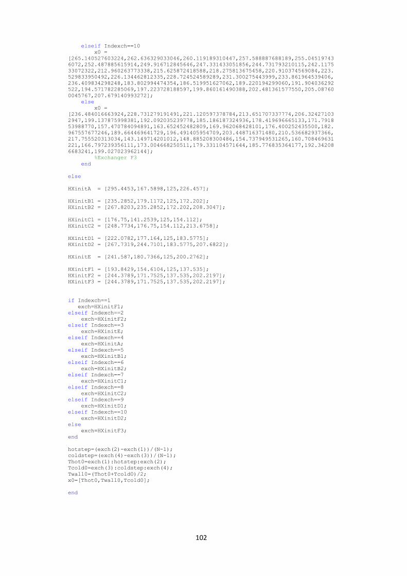
102
elseif Indexch==10
x0 =
[265.140527603224,262.636329033046,260.119189310447,257.588887688189,255.04519743
6072,252.487885615914,249.916712845646,247.331433051856,244.731793210115,242.1175
33072322,212.960263773338,215.625872418588,218.275813675458,220.910374569084,223.
529833950492,226.134462812335,228.724524589289,231.300275443999,233.861964539406,
236.409834298248,183.802994474354,186.519951627062,189.220194299060,191.904036292
522,194.571782285069,197.223728188597,199.860161490388,202.481361577550,205.08760
0045767,207.679140993272];
else
x0 =
[236.484016663924,228.731279191491,221.120597378784,213.651707337774,206.32427103
2947,199.137875998381,192.092035239778,185.186187324936,178.419696665133,171.7918
53988770,157.470784094891,163.652452482809,169.962068428101,176.400252435500,182.
967557677246,189.664469641729,196.491405954709,203.448716371480,210.536682937366,
217.755520313034,143.149714201012,148.885208300486,154.737949531265,160.708469631
221,166.797239356111,173.004668250511,179.331104571644,185.776835364177,192.34208
6683241,199.027023962144];
%Exchanger F3
end
else
HXinitA = [295.4453,167.5898,125,226.457];
HXinitB1 = [235.2852,179.1172,125,172.202];
HXinitB2 = [267.8203,235.2852,172.202,208.3047];
HXinitC1 = [176.75,141.2539,125,154.112];
HXinitC2 = [248.7734,176.75,154.112,213.6758];
HXinitD1 = [222.0782,177.164,125,183.5775];
HXinitD2 = [267.7319,244.7101,183.5775,207.6822];
HXinitE = [241.587,180.7366,125,200.2762];
HXinitF1 = [193.8429,154.6104,125,137.535];
HXinitF2 = [244.3789,171.7525,137.535,202.2197];
HXinitF3 = [244.3789,171.7525,137.535,202.2197];
if Indexch==1
exch=HXinitF1;
elseif Indexch==2
exch=HXinitF2;
elseif Indexch==3
exch=HXinitE;
elseif Indexch==4
exch=HXinitA;
elseif Indexch==5
exch=HXinitB1;
elseif Indexch==6
exch=HXinitB2;
elseif Indexch==7
exch=HXinitC1;
elseif Indexch==8
exch=HXinitC2;
elseif Indexch==9
exch=HXinitD1;
elseif Indexch==10
exch=HXinitD2;
else
exch=HXinitF3;
end
hotstep=(exch(2)-exch(1))/(N-1);
coldstep=(exch(4)-exch(3))/(N-1);
Thot0=exch(1):hotstep:exch(2);
Tcold0=exch(3):coldstep:exch(4);
Twall0=(Thot0+Tcold0)/2;
x0=[Thot0,Twall0,Tcold0];
end
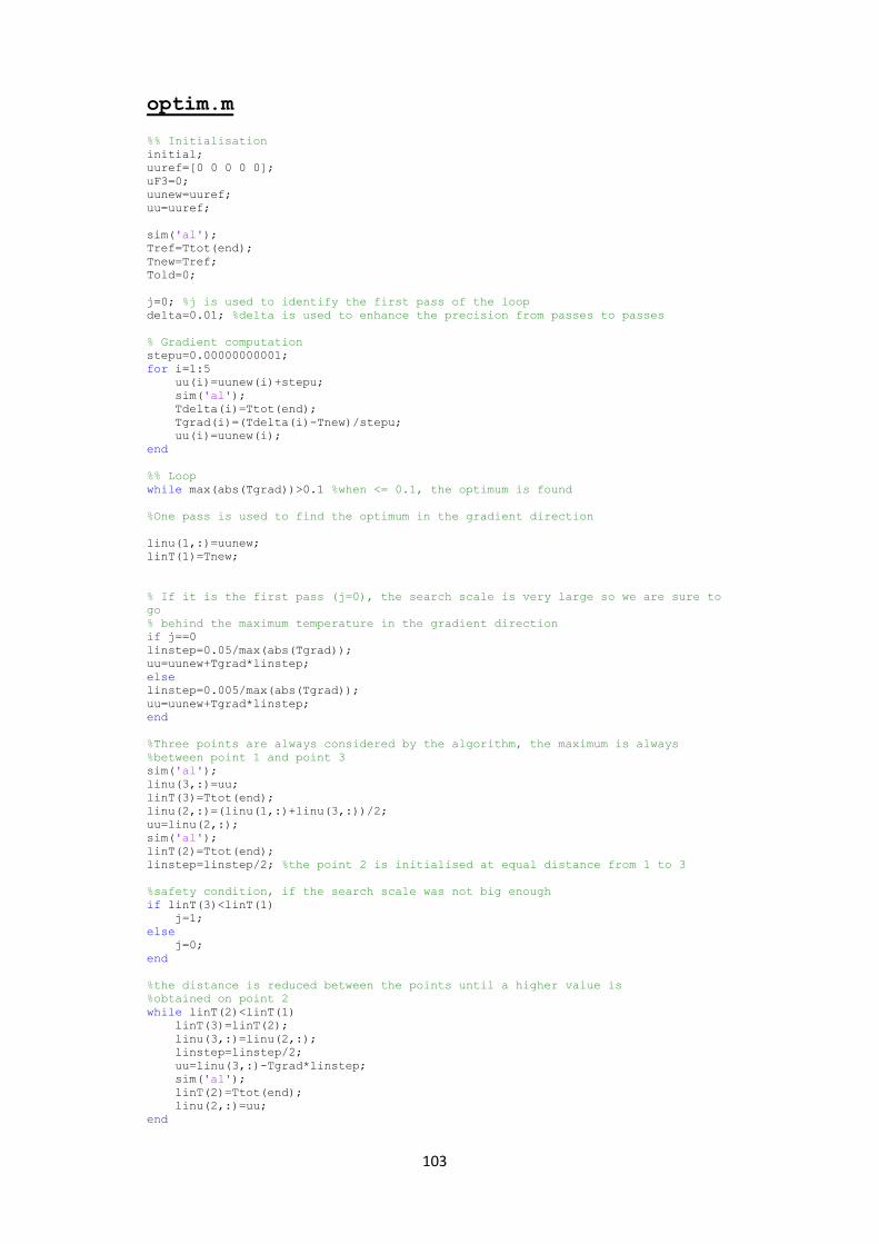
103
optim.m
%% Initialisation
initial;
uuref=[0 0 0 0 0];
uF3=0;
uunew=uuref;
uu=uuref;
sim('al');
Tref=Ttot(end);
Tnew=Tref;
Told=0;
j=0; %j is used to identify the first pass of the loop
delta=0.01; %delta is used to enhance the precision from passes to passes
% Gradient computation
stepu=0.00000000001;
for i=1:5
uu(i)=uunew(i)+stepu;
sim('al');
Tdelta(i)=Ttot(end);
Tgrad(i)=(Tdelta(i)-Tnew)/stepu;
uu(i)=uunew(i);
end
%% Loop
while max(abs(Tgrad))>0.1 %when <= 0.1, the optimum is found
%One pass is used to find the optimum in the gradient direction
linu(1,:)=uunew;
linT(1)=Tnew;
% If it is the first pass (j=0), the search scale is very large so we are sure to
go
% behind the maximum temperature in the gradient direction
if j==0
linstep=0.05/max(abs(Tgrad));
uu=uunew+Tgrad*linstep;
else
linstep=0.005/max(abs(Tgrad));
uu=uunew+Tgrad*linstep;
end
%Three points are always considered by the algorithm, the maximum is always
%between point 1 and point 3
sim('al');
linu(3,:)=uu;
linT(3)=Ttot(end);
linu(2,:)=(linu(1,:)+linu(3,:))/2;
uu=linu(2,:);
sim('al');
linT(2)=Ttot(end);
linstep=linstep/2; %the point 2 is initialised at equal distance from 1 to 3
%safety condition, if the search scale was not big enough
if linT(3)<linT(1)
j=1;
else
j=0;
end
%the distance is reduced between the points until a higher value is
%obtained on point 2
while linT(2)<linT(1)
linT(3)=linT(2);
linu(3,:)=linu(2,:);
linstep=linstep/2;
uu=linu(3,:)-Tgrad*linstep;
sim('al');
linT(2)=Ttot(end);
linu(2,:)=uu;
end
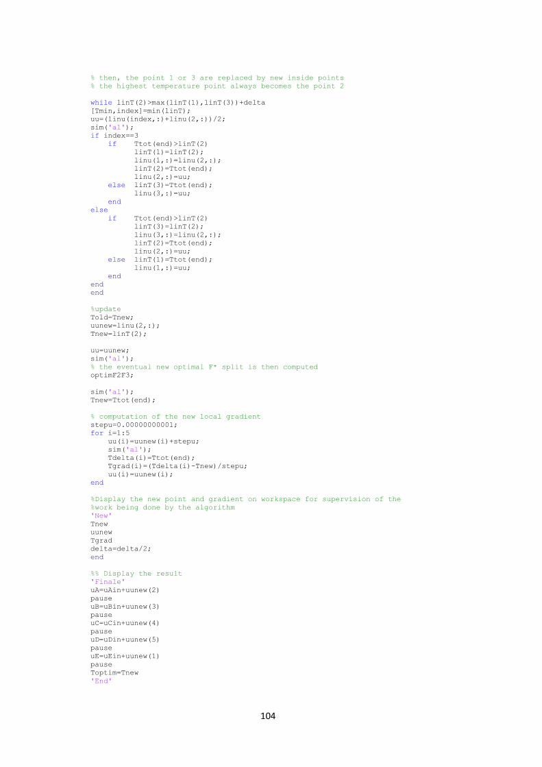
104
% then, the point 1 or 3 are replaced by new inside points
% the highest temperature point always becomes the point 2
while linT(2)>max(linT(1),linT(3))+delta
[Tmin,index]=min(linT);
uu=(linu(index,:)+linu(2,:))/2;
sim('al');
if index==3
if Ttot(end)>linT(2)
linT(1)=linT(2);
linu(1,:)=linu(2,:);
linT(2)=Ttot(end);
linu(2,:)=uu;
else linT(3)=Ttot(end);
linu(3,:)=uu;
end
else
if Ttot(end)>linT(2)
linT(3)=linT(2);
linu(3,:)=linu(2,:);
linT(2)=Ttot(end);
linu(2,:)=uu;
else linT(1)=Ttot(end);
linu(1,:)=uu;
end
end
end
%update
Told=Tnew;
uunew=linu(2,:);
Tnew=linT(2);
uu=uunew;
sim('al');
% the eventual new optimal F* split is then computed
optimF2F3;
sim('al');
Tnew=Ttot(end);
% computation of the new local gradient
stepu=0.00000000001;
for i=1:5
uu(i)=uunew(i)+stepu;
sim('al');
Tdelta(i)=Ttot(end);
Tgrad(i)=(Tdelta(i)-Tnew)/stepu;
uu(i)=uunew(i);
end
%Display the new point and gradient on workspace for supervision of the
%work being done by the algorithm
'New'
Tnew
uunew
Tgrad
delta=delta/2;
end
%% Display the result
'Finale'
uA=uAin+uunew(2)
pause
uB=uBin+uunew(3)
pause
uC=uCin+uunew(4)
pause
uD=uDin+uunew(5)
pause
uE=uEin+uunew(1)
pause
Toptim=Tnew
'End'

105
optimF2F3.m
%optimF2F3, same principle than the algorithm for the multivariable split
A,B,C,D,E,F
TF2b=ToutF2tot(end);
TnewF2=TF2b;
uF3b=uF3;
uF3a=uF3b-0.1;
uF3=uF3a;
sim('al');
TF2a=ToutF2tot(end);
uF3c=uF3b+0.1;
uF3=uF3c;
sim('al');
TF2c=ToutF2tot(end);
linTF2=[TF2a TF2b TF2c];
linuF2=[uF3a uF3b uF3c];
while linTF2(2)>max(linTF2(1),linTF2(3))+0.01
[TminF2,indexF2]=min(linTF2);
uF3=(linuF2(indexF2)+linuF2(2))/2;
sim('al');
if indexF2==3
if ToutF2tot(end)>linTF2(2)
linTF2(1)=linTF2(2);
linuF2(1)=linuF2(2);
linTF2(2)=ToutF2tot(end);
linuF2(2)=uF3;
else linTF2(3)=ToutF2tot(end);
linuF2(3)=uF3;
end
else
if ToutF2tot(end)>linTF2(2)
linTF2(3)=linTF2(2);
linuF2(3)=linuF2(2);
linTF2(2)=ToutF2tot(end);
linuF2(2)=uF3;
else linTF2(1)=ToutF2tot(end);
linuF2(1)=uF3;
end
end
end
%update
ToldF2=TnewF2;
uF3new=linuF2(2);
TnewF2=linTF2(2);
uF3=uF3new;