heat and fluid flow characterization of a single-hole-per
TRANSCRIPT

University of Central Florida University of Central Florida
STARS STARS
Electronic Theses and Dissertations, 2004-2019
2013
Heat And Fluid Flow Characterization Of A Single-hole-per-row Heat And Fluid Flow Characterization Of A Single-hole-per-row
Impingement Channel At Multiple Impingement Heights Impingement Channel At Multiple Impingement Heights
Roberto Claretti University of Central Florida
Part of the Mechanical Engineering Commons
Find similar works at: https://stars.library.ucf.edu/etd
University of Central Florida Libraries http://library.ucf.edu
This Masters Thesis (Open Access) is brought to you for free and open access by STARS. It has been accepted for
inclusion in Electronic Theses and Dissertations, 2004-2019 by an authorized administrator of STARS. For more
information, please contact [email protected].
STARS Citation STARS Citation Claretti, Roberto, "Heat And Fluid Flow Characterization Of A Single-hole-per-row Impingement Channel At Multiple Impingement Heights" (2013). Electronic Theses and Dissertations, 2004-2019. 2936. https://stars.library.ucf.edu/etd/2936

HEAT AND FLUID FLOW CHARACTERIZATION OF A SINGLE-HOLE-PER-ROW
IMPINGEMENT CHANNEL AT MULTIPLE IMPINGEMENT HEIGHTS
by
ROBERTO CLARETTI
B.S. University of Central Florida, 2011
A thesis submitted in partial fulfillment of the requirements
for the degree of Master of Science
in the Department of Mechanical and Aerospace Engineering
in the College of Engineering and Computer Science
at the University of Central Florida
Orlando, Florida
Fall Term
2013
Major Professor: Jayanta Kapat

ii
© 2013 Roberto Claretti

iii
ABSTRACT
The present work studies the relationship between target and sidewall surfaces of a multi-
row, narrow impingement channel at various jet heights with one impingement hole per row.
Temperature sensitive paint and constant flux heaters are used to gather heat transfer data on the
target and side walls. Jet-to-target distance is set to 1, 2, 3, 5, 7 and 9 jet diameters. The channel
width is 4 jet diameters and the jet stream wise spacing is 5 jet diameters. All cases were run at
Reynolds numbers ranging from 5,000 to 30,000. Pressure data is also gathered and used to
calculate the channel mass flux profiles, used to better understand the flow characteristics of the
impingement channel. While target plate heat transfer profiles have been thoroughly studied in
the literature, side wall data has only recently begun to be studied. The present work shows the
significant impact the side walls provide to the overall heat transfer capabilities of the
impingement channel. It was shown that the side walls provide a significant amount of heat
transfer to the channel. A channel height of three diameters was found to be the optimum height
in order to achieve the largest heat transfer rates out of all channels.

iv
DEDICATED TO ENNIO, MAMA Y PAPA.
To those with a never-ending thirst for knowledge

v
ACKNOWLEDGMENTS
Special thanks to my thesis chair Dr. Kapat; your advice has been invaluable. I would
also like to thank the rest of my committee members, Dr. Raghavan, Dr. Vasu and Dr. Kassab.
I would like to acknowledge the help I received from John Harrington on the final phases
of testing and the help Joshua Bernstein and Jahed Hossain have given me. Thanks to everyone I
worked with on FCFC: Greg Natsui, Constantine Wolski, Justin Hodges, Jonathan Allred, Mark
Miller and Orlando Ardila. Thanks to Anthony Bravato for keeping the lab together; thanks to
Matt Golsen, Mark Ricklick, Lucky Tran, Abhishek Saha, Perry Johnson and Carson Slabaugh
for answering the questions I had and engaging in thoughtful discussions about all aspects of
turbomachinery and life in general.
Thanks to Jim Downs, Gloria Goebel, An Lee, Michelle Valentino and Bryan Bernier for
their kind hospitality over my internship at FTT. Thanks again to Mark Ricklick and everyone
else at CD-Adapco for showing me how to work with StarCCM+.
More recently I would like to thank everyone at GRC including Brian Barr, Jon Slepski,
Jeff Doom, Suranga Dharmarathne, and Greg Natsui again! for making my stay as a GRC intern
memorable.

vi
TABLE OF CONTENTS
LIST OF FIGURES ........................................................................................................ viii
LIST OF TABLES ............................................................................................................ xi
LIST OF NOMENCLATURE ........................................................................................ xii
CHAPTER ONE: INTRODUCTION ................................................................................. 1
Gas Turbine as a Heat Engine ......................................................................................... 1
Cooling of Gas Turbine Hot Components ...................................................................... 4
CHAPTER TWO: LITERATURE REVIEW ..................................................................... 5
Impingement Heat Transfer ............................................................................................ 5
Numerical Impingement Heat Transfer .......................................................................... 5
Single Round Nozzle Impingement Heat Transfer ......................................................... 7
Impingement Flow Visualization .................................................................................... 9
Impingement Arrays ..................................................................................................... 10
Impingement Heat Transfer Reviews ........................................................................... 14
Other Impingement Literature ...................................................................................... 15
Experimental Techniques.............................................................................................. 17
CHAPTER THREE: PURPOSE AND PROBLEM STATEMENT ................................ 18
CHAPTER FOUR: EXPERIMENTAL SETUP AND DATA REDUCTION ................. 20
Data Reduction.............................................................................................................. 27

vii
Lateral Conduction Estimation ..................................................................................... 32
CHAPTER FIVE: EXPERIMENTAL UNCERTAINTY ................................................ 34
CHAPTER SIX: FLOW RESULTS ................................................................................. 37
CHAPTER SEVEN: HEAT TRANSFER RESULTS ...................................................... 39
Smooth Channel Validation .......................................................................................... 39
Heat Transfer Results .................................................................................................... 40
CHAPTER EIGHT: HEAT TRANSFER DATA ANALYSIS ........................................ 48
Nusselt Number Dependence of Reynolds number ...................................................... 48
Total Heat Transfer Contribution.................................................................................. 50
Comparisons with Florschuetz et al. [18] Correlation .................................................. 52
CHAPTER NINE: CONCLUSIONS ................................................................................ 55
APPENDIX A: NUSSELT NUMBER PROFILES .......................................................... 56
APPENDIX B: SPAN AVERAGED NUSSELT NUMBER DATA ............................... 62
APPENDIX C: TABULATED NUSSELT NUMBER DATA ........................................ 69
APPENDIX D: ACTUAL REYNOLDS NUMBERS ...................................................... 76
APPENDIX E: LATERAL CONDUCTION CALCULATIONS .................................... 78
REFERENCES ................................................................................................................. 81

viii
LIST OF FIGURES
Figure 1: Energy Consumption in Electricity Generation (1015
BTU) ........................................... 1
Figure 2: Energy Uses in the United States and their Respective Sources. .................................... 2
Figure 3: Turbine airfoil cooled with a series of impingement channel with heat paths showing
importance of side wall heat transfer .......................................................................... 19
Figure 4: Isometric view of Z/D=1 impingement channel CAD .................................................. 21
Figure 5: Impingement channel geometric parameters ................................................................. 21
Figure 6: Impingement channel flow loop and camera setup ....................................................... 22
Figure 7: Temperature sensitive paint calibration setup ............................................................... 25
Figure 8: Temperature sensitive paint calibration results and comparisons with older correlations
..................................................................................................................................... 26
Figure 9: 1D diagram of test section layers (not drawn to scale) ................................................. 27
Figure 10: Conduction Loss Diagram ........................................................................................... 28
Figure 11: Heat loss results and correlation .................................................................................. 29
Figure 12: Sample Pressure Profile............................................................................................... 30
Figure 13: Lateral Conduction Estimates ..................................................................................... 33
Figure 14: Absolute Uncertainties of Nusselt Number ................................................................. 35
Figure 15: Absolute Uncertainties of Reynolds Number .............................................................. 36
Figure 16: Channel mass flux to jet mass flux ratio distribution .................................................. 37
Figure 17: Local jet mass flux to average jet mass flux ratio and comparisons to analytical
models ......................................................................................................................... 38
Figure 18: Smooth Channel Validation ........................................................................................ 40

ix
Figure 19: Target Wall Comparison at Rejavg=10,000 .................................................................. 42
Figure 20: Target Wall Comparison at Rejavg=15,000 .................................................................. 42
Figure 21: Side Wall Comparison at Rejavg=10,000 ..................................................................... 43
Figure 22: Side Wall Comparison at Rejavg=15,000 ..................................................................... 44
Figure 23: Target Wall Nusselt number Comparisons at Rejavg=15,000 ...................................... 45
Figure 24: Side Wall Nusselt number Comparisons at Rejavg=15,000 .......................................... 45
Figure 25: Isometric View of all Channels at Rejavg=10,000 ........................................................ 47
Figure 26: Isometric View of all Channels at Rejavg=15,000 ........................................................ 47
Figure 27: Variation of Reynolds Number Exponent, "m", as a Function of Wall and Channel
Height .......................................................................................................................... 49
Figure 28: Contributions of Target and Side Walls on Overall Channel Heat Transfer for
Rejavg=10,000 .............................................................................................................. 51
Figure 29: Contributions of Target and Side Walls on Overall Channel Heat Transfer for
Rejavg=15,000 .............................................................................................................. 52
Figure 30: Z/D = 2 Nusselt Number Profile Comparisons with Florschuetz et al. ....................... 53
Figure 31: Z/D = 3 Nusselt Number Profile Comparisons with Florschuetz et al. ....................... 54
Figure 32: Z/D=1 Target Wall Nusselt number Profiles at Multiple Reynolds Numbers ............ 57
Figure 33: Z/D=2 Target Wall Nusselt number Profiles at Multiple Reynolds Numbers ............ 57
Figure 34: Z/D=3 Target Wall Nusselt number Profiles at Multiple Reynolds Numbers ............ 57
Figure 35: Z/D=5 Target Wall Nusselt number Profiles at Multiple Reynolds Numbers ............ 58
Figure 36: Z/D=7 Target Wall Nusselt number Profiles at Multiple Reynolds Numbers ............ 58
Figure 37: Z/D=9 Target Wall Nusselt number Profiles at Multiple Reynolds Numbers ............ 58
Figure 38: Z/D=1 Side Wall Nusselt number Profiles at Multiple Reynolds Numbers ............... 59

x
Figure 39: Z/D=2 Side Wall Nusselt number Profiles at Multiple Reynolds Numbers ............... 59
Figure 40: Z/D=3 Side Wall Nusselt number Profiles at Multiple Reynolds Numbers ............... 59
Figure 41: Z/D=5 Side Wall Nusselt number Profiles at Multiple Reynolds Numbers ............... 60
Figure 42: Z/D=7 Side Wall Nusselt number Profiles at Multiple Reynolds Numbers ............... 60
Figure 43: Z/D=9 Side Wall Nusselt number Profiles at Multiple Reynolds Numbers ............... 61
Figure 44: Target Wall Laterally Averaged Nusselt Number for Z/D=1 ..................................... 63
Figure 45: Side Wall Laterally Averaged Nusselt Number for Z/D=1 ......................................... 63
Figure 46: Target Wall Laterally Averaged Nusselt Number for Z/D=2 ..................................... 64
Figure 47: Wall Laterally Averaged Nusselt Number for Z/D=2 ................................................. 64
Figure 48: Target Wall Laterally Averaged Nusselt Number for Z/D=3 ..................................... 65
Figure 49: Wall Laterally Averaged Nusselt Number for Z/D=3 ................................................. 65
Figure 50: Target Wall Laterally Averaged Nusselt Number for Z/D=5 ..................................... 66
Figure 51: Wall Laterally Averaged Nusselt Number for Z/D=5 ................................................. 66
Figure 52: Target Wall Laterally Averaged Nusselt Number for Z/D=7 ..................................... 67
Figure 53: Wall Laterally Averaged Nusselt Number for Z/D=7 ................................................. 67
Figure 54: Target Wall Laterally Averaged Nusselt Number for Z/D=9 ..................................... 68
Figure 55: Wall Laterally Averaged Nusselt Number for Z/D=9 ................................................. 68

xi
LIST OF TABLES
Table 1: Florschuetz Correlation Constants for an Inline Array ................................................... 11
Table 2: Test Matrix...................................................................................................................... 23
Table 3: Absolute and Relative Nusselt Number Uncertainties ................................................... 34
Table 4: Absolute and Relative Reynolds Number Uncertainties ................................................ 35
Table 5: Nusselt Number Dependence on Reynolds Number ...................................................... 48
Table 6: Total Channel Heat Transfer .......................................................................................... 50
Table 7: Z/D=1 Target Wall Pitch Averaged Nusselt Number .................................................... 70
Table 8: Z/D=1 Side Wall Pitch Averaged Nusselt Number ........................................................ 70
Table 9: Z/D=2 Target Wall Pitch Averaged Nusselt Number .................................................... 71
Table 10: Z/D=2 Side Wall Pitch Averaged Nusselt Number ...................................................... 71
Table 11: Z/D=3 Target Wall Pitch Averaged Nusselt Number .................................................. 72
Table 12: Z/D=3 Side Wall Pitch Averaged Nusselt Number ...................................................... 72
Table 13: Z/D=5 Target Wall Pitch Averaged Nusselt Number .................................................. 73
Table 14: Z/D=5 Side Wall Pitch Averaged Nusselt Number ...................................................... 73
Table 15: Z/D=7 Target Wall Pitch Averaged Nusselt Number .................................................. 74
Table 16: Z/D=7 Side Wall Pitch Averaged Nusselt Number ...................................................... 74
Table 17: Z/D=9 Target Wall Pitch Averaged Nusselt Number .................................................. 75
Table 18: Z/D=9 Side Wall Pitch Averaged Nusselt Number ...................................................... 75
Table 19: Actual Reynolds Numbers ............................................................................................ 77

xii
LIST OF NOMENCLATURE
Cross Sectional Area
Heater Surface Area (m2)
Specific Heat at Constant Pressure (kJ/kg K)
D Jet Diameter (m)
Channel Hydraulic Diameter (m)
Heat Transfer Coefficient (HTC) (W/m2
K)
Average Heat Transfer Coefficient (W/m2
K)
k Thermal Conductivity (W/m K)
Channel Length (m)
Mass Flow Rate (kg/s)
Nu Nusselt Number
Static Pressure (kPa)
Total Pressure (kPa)
Pr Prandtl Number
Heat Flux (W/m2)
Total Heat Input (W)
Heater Resistance (ohm)
Re Reynolds Number
SW Side Wall
Temperature (K)
TW Target Wall

xiii
Voltage Potential
Streamwise Location
y Spanwise Location
z Height from Target Wall
X Streamwise Distance (m)
Y Spanwise Distance (m)
Z Impingement Height (m)
Ratio of Specific Heats
Air Density (kg/m3)
Subscripts
C Cold
cs Cross-section
ch Channel
Carnot Describing a Carnot cycle
Exit
Effective
H Hot
javg Average jet quantity (applicable to Re)
Quantity Lost to the Environment
Reference Value
Wall Value
Base Line Value or Total Quantity

1
CHAPTER ONE: INTRODUCTION
Gas Turbine as a Heat Engine
Gas turbines power all commercial and military aircraft as well as provide a quarter of
the electricity generated in the United States [1]. With the rising environmental, political and fuel
cost of the operation of these engines, users are seeking to increase their efficiency. To put
electricity generation into perspective, Figure 1 shows the total amount of energy used in the
generation of electrical power in the United States. A total of 40.04 quadrillion BTUs are used to
generate 14.82 quadrillion BTUs of electrical power ─ a conversion rate of 37%. Out of the
40.04 quadrillion BTUs of total energy used, 8.05 quadrillion BTUs come from natural gas, the
primary fuel power generation gas turbines operate on. Jet fuel accounts for 7.6% of the
petroleum consumption in the US at 1.43 million barrels per day [1]. The scale of energy use in
the United States displays the major benefits obtainable from an increase of efficiency of gas
turbine engines.
Figure 1: Energy Consumption in Electricity Generation (1015
BTU)

2
Source: DOE U.S. Energy Information Administration Annual Energy Review
http://www.eia.gov/totalenergy/data/annual/pdf/aer.pdf
Figure 2: Energy Uses in the United States and their Respective Sources.
Source: Lawrence Livermore National Laboratory Energy Flow Charts
https://flowcharts.llnl.gov/
Contrary to the chart shown in Figure 1, which only shows the flow of energy used in the
generation of electrical power, Figure 2 also contains energy used for transportation. It can be
seen that transportation is the main user of petroleum products. Transportation features the
lowest conversion efficiency out of all sources of energy at a meager 21%. Gas turbines are used
to power some modes of transportation including all commercial and military aircraft and some
sea vessels; increasing the efficiency of these engines not only decreases the cost of electricity
but also decreases the cost of some modes of transportation.

3
Gas turbines are modeled thermodynamically by the Brayton Cycle. The cycle entails
three main processes that can be directly ties to different parts of a gas turbine. Pressure is
increased in the compressor; heat is added by combusting natural gas or gasified coal on power
generation engines and jet fuel on aviation engines; energy is then extracted from the working
fluid (post combustion gasses) in the turbine which provides power to the compressor and to the
generator on power generation gas turbines and to the compressor and fan on aviation engines.
The exhaust is the deposited in the atmosphere for all aviation engines and simple cycle power
generation engines; for combined cycle power generation, the exhaust gases are fed through a
heat recovery steam generator, or HRSG, where, as the name describes, some of the remaining
heat from the post-combustion gasses is transferred to steam which is then used to power steam
turbines. The use of the waste heat drastically improves the overall efficiency of the power plant.
The isentropic efficiency of Brayton Cycle engines is given by
(1)
Using the isentropic efficiency to determine what aspect of a real engine should be
improved is appropriate due to the fact that even if the real engine efficiency cannot be
determined using the isentropic efficiency, an increase in isentropic efficiency will be reflected
in the real engine efficiency. It is therefore possible to analyze the Brayton cycle using the
isentropic efficiency to determine possible improvements. A decrease in T1 would increase the
efficiency; however, since T1 is the atmospheric temperature, engineers have little control of it
other than location of certain power plant, or the cruising altitude of an airliner. The other option
engineers have is to increase the turbine inlet temperature, T3. The problem in increasing the
turbine inlet temperature is that the current temperature gas turbines operate on is higher than the
melting point of the materials that they are made out of [2], [3], [4]. Current gas turbines are
4
cooled with compressor bypass air that flow through cooling channels in the turbine blades and
vanes as well as in the transition duct; the cooling air is the bled out onto the hot surfaces as film
cooling which provides a cooling blanket of air protecting the surface from the hot gasses.
Cooling alone is not sufficient enough to assure the reliable operation of gas turbine hot
components. Designers employ the use of nickel-based super alloys which are coated with
thermal barrier coatings. It is the combination of the high-temperature capable super alloys,
thermal barrier coatings and internal and external cooling that allow the continuous operation of
the critical components in the harsh environment.
Cooling of Gas Turbine Hot Components
Gas turbine blades are cooled multiple ways depending on the manufacturer. Early
versions of cooled blades only contained radial convective cooling channels. As time progressed,
cooling technologies as well as better super alloys and thermal barrier coatings were developed
and deployed. Modern blades are cooled with serpentine channels in the midchord region lined
with turbulators to enhance their heat transfer capability, pin fin arrays located in the trailing
edge region and impingement cooling coupled with showerhead cooling on the leading edge.
Vanes, or stators, are cooled with an array of impinging jets generated by a jet-inducing insert.
The vanes are also lined with showerhead cooling holes on the leading edge and film cooling
holes on the pressure and suction sides was well as on both endwalls. Transition ducts are cooled
with channels lined with turbulators as well as impingement and multiple rows of film cooling.
Designers have begun to take advantage of the cooling capability of impingement due to the
large heat transfer coefficients it generates at a given coolant mass flow rate.

5
CHAPTER TWO: LITERATURE REVIEW
Impingement Heat Transfer
Impingement cooling has been researched since the early 1960s. Hundreds of papers have
been published describing the heat transfer and flow characteristics of single round nozzle
impingement, staggered and inline impingement arrays, impingement on curved surfaces to
simulate the ones found on a leading edge, angled impingement, swirling jets, impingement on
surfaces with porous foam and turbulators, flow visualization, coupled impingement-effusion,
effects of nozzle geometry and multiple other geometric, flow or heat transfer studies.
Due to the large breadth of literature on impingement cooling, only relevant work to the
present study as well as multiple cornerstone studies on impingement heat transfer are discussed
in detail.
Numerical Impingement Heat Transfer
Multiple works have studied numerical simulations of impingement heat transfer. El-
Gabry [5] performed a numerical investigation of an impingement channel which consisted of 8
streamwise holes. The paper investigated the Nusselt number prediction differences between two
different turbulence models; the Yang-Shih and standard k-ε. Computational results were
compared to experimental results obtained previously. Two channel heights were tested of 1 and 2 jet
diameters; three jet inclinations were also tested at 30, 60 ad 90 degrees off of the target wall normal.
The deviation of Nusselt number between the experimental and computational results were
calculated The Yang-Shih turbulence model predicted well at low Reynolds numbers as the area
averaged Nusselt number being 5% off from the experimental value while the standard k-ε was off
by 9.4%. As jet Reynolds number was increased, the error of the standard k-ε model dropped to as
low as 3.9% higher than the experimental data while the error from the Yang-shih model increased to

6
7.6% below the experimental average. Plots containing experimental and computational span-
averaged Nusselt number results are shown. A peak of Nusselt number is predicted by both codes
directly beneath the stagnation region; however, the magnitude of the span-averaged Nusselt number
profile of both numerical solutions is higher than the experimental one. The amplitude of fluctuations
is greater for the CFD solutions; it is important to note that even though the error in average Nusselt
number is not great, the actual differences in the profile are much greater; upwards of 20% difference
of heat transfer coefficients between the experimental and numerical heat transfer peaks. Such
discrepancy may not be entirely due to numerical errors and/or the inability for either turbulence
model to predict the heat transfer at the stagnation regions; it may also be caused to potential lateral
conduction on the experimental side.
Zuckerman, et al. [6] compared a much wider array of turbulence models in their ability
to predict Nusselt numbers caused by jet impingement. The models tested were k – ε, k-ω,
Reynolds Stress Model, algebraic stress models, shear stress transport and lastly, the υ2f
turbulence model. Large eddy simulation was run as the only time-dependent turbulence model.
The paper summarizes all the different models used, their computational cost, impingement
Nusselt number, and their ability to predict the secondary peak encountered at low impingement
heights. As expected LES provide the best prediction of both stagnation and secondary peak heat
transfer coefficient; however, this comes at a large computational cost. The k–ε and k-ω provide
poor heat transfer results for the stagnation region where they can have 30% error from the
correct value. The realizable k–ε model provides better heat transfer results while still
maintaining a low computational cost. The highest accuracy to cost ratio was achieved by the υ2f
model where it predicts the heat transfer coefficient for the surface with a minimum of 2% error
while not being as expensive as the other unsteady models such as DNS and LES.

7
Mushatat [7] performed basic 2-D computational studies on a slot impingement channel
with initial crossflow. Multiple numbers of slot jets were studied as well as rib features on the
target wall. Nusselt number plots were shown and discussed with little comparison of the results
with previous literature. The work shows an increase in target wall heat transfer with an increase
in slot velocity at constant crossflow velocity; an increase of the ratio of slot jet width to rib
thickness yielded an increase in Nusselt number.
Taslim, et al. [8] investigated numerically and experimentally the heat transfer
characteristics of jet impingement on a curved leading edge surface with and without ribs. The
highest area average convective coefficients were found on the rib-less geometry. One of the
ribbed geometries tested yielded the highest rate of heat transfer due to the increased wetted area
- a result commonly found on internal cooling enhancement with the use of rib turbulators.
Acharya, et al. [9] examined velocity profiles generated by the exhaust of flow incoming though
a circular tube into a crossflow similar to geometries seen in showerhead film cooling. Incoming
flow carried a preset velocity which decreased as flow was removed from it as it exited through
orifices on the tube. Velocity profiles for flow though each orifice is shown and are used to
understand the different jet velocity profiles generated with varying crossflow conditions.
Single Round Nozzle Impingement Heat Transfer
Single round nozzle impingement consists of a single jet impinging a surface with the
spent air exiting in the radial direction. Multiple variations have been studied in the literature.
Gulati, et al. [10] studied the effect of different nozzle shapes including round, square, and
rectangular nozzle at Z/D of 0.5, 1, 2, 4, 6, 8, 10, and 12 with D being he hydraulic diameter of
the respective jet. The Nusselt number profile closely resembled the shape of the nozzle at low

8
impingement heights; however, as the impingement height increased, the profile lost its shape as
the jet lost its momentum by diffusion. Rectangular jets were found to have radialy varying
profiles even at large impingement heights. The Reynolds number dependence of Nusselt
number was not found to be altered by nozzle shape implying the hydraulic diameter correctly
predicted the length scale of the different shaped jets. The pressure loss due to the jet formation
and impingement was found to be lowest for the circular shape and highest for the rectangular
shape – this result is expected due to the jets being allowed to develop for 50 jet hydraulic
diameters, causing a large pressure drop on the rectangular jet due to the larger wetted area.
Herrero-Martin et al. [11] studied two types of nozzle shapes and their effect on target wall
Nusselt number distribution. The two different nozzles consisted of the intersection of three
circular profiles located at the three vertices of an equilateral triangle with a side length equal to
the diameter of the circles and the intersection of four circular jets whose center was located on
each corner of a square whose side was slightly smaller than the diameter of the jets; they are
named triangular nozzle and quadrangular nozzle respectively. Several impingement heights
were tested Z/D = 1, 2, 3, 4, 5, 6, 7, and 12. The performance of the different nozzles were found
to be a function of Reynolds number; at a Reynolds number greater than 15,000, the
quadrangular nozzle delivered the highest rate of heat transfer while the triangular nozzle
performed better at Reynolds numbers less than 15,000. Lee, et al. [12] studied round nozzles
with variations of the finish on the flow side of the jet-issuing-plate. Three geometries were
tested, one with a square edged exit, one with a chamfered exit and one with a sharp exit. The
thickness of the jet-issuing-plate was 1/5 of the jet diameter, L/D=1/5. Multiple impingement
heights were tested Z/D = 2, 4, 6, and 10. The Nusselt number dependence factor on Reynolds
number was found not to be a function of nozzle finish. Slight variations in the area averaged

9
Nusselt number were found with varying nozzle finish. The authors provided Nusselt number
correlations for all three nozzle finishes. The nozzle with the square exit was found to be the
most beneficial due to it scaling at a higher rate with an increase of Reynolds number.
Other work on single round nozzle impingement is given in literature reviews, most
notably in Martin [13], Viskanta [14], and Weigand et al. [15]. These works are discussed in
more detail in the impingement review section.
Impingement Flow Visualization
Carcasci [16] used multiple flow visualization techniques to study the resulting flow field
caused by numerous types of impingement geometries. The techniques used included oil and
pigment on a wall (target wall in this case), thermo-tropic liquid crystal on a wall as well as a
simple smoke flow test. The different geometries tested included a single round nozzle
impingement, inline jet interactions (similar to the geometry studied in this work) inline jet
interaction with the effect of crossflow and finally, a geometry consisting 9 jets in a square
pattern with crossflow. The paper explains the difference in secondary vortices generated
between a jet impinging on a surface with and without crossflow. The addition of crossflow
causes the main wall jet from an upstream jet to separate from the wall as it meets the wall jet
caused by a jet impinging directly downstream causing an effect similar to a hydraulic jump in
the wall jet stagnation region. The high turbulence shown in this region is used to explain
relatively higher convective coefficients when compared to regions of wall jets with no
interaction with other flows. The study does not take into account side walls used in the inline
cases; it would be beneficial for future impingement researchers to study the flow behavior at the

10
side walls (with oil and dye) in order to better understand the interaction of the wall jet and the
side wall and its effect on heat transfer.
Impingement Arrays
Among the most well known impingement heat transfer studies lays the Florschuetz, et
al. NASA technical reports and corresponding journal articles [17],[18] and[19] (at the time of
writing, the NASA reports have been taken down from the NASA FOIA website).The research
done by Florschuetz et al. studied an impingement array with the purpose of finding the optimum
lateral and streamwise jet spacing, Y/D and X/D respectively, in order to maximize the target
wall heat transfer. Jet-to-target wall spacing, Z/D ranged from 1 to 3, the streamwise spacings
tested were X/D=5, 10 and 15 while the lateral spacing was kept at Y/D 4, 6 and 8. Florschuetz’s
et al. major contribution was the development of a correlation which provided a relationship
between jet area average Nusselt number as a function of flow and geometric parameters. The
correlation takes the form
(2)
with A, m, B and n being functions of geometric parameters calculated using the following
correlation
(3)
The constants C, nx, ny, and nz are given in Table 1 for an inline array

11
Table 1: Florschuetz Correlation Constants for an Inline Array
C nx ny nz
A 1.18 -0.944 -0.642 0.169
m 0.612 0.059 0.032 -0.022
B 0.437 -0.095 -0.219 0.275
n 0.092 -0.005 0.599 1.04
Florschuetz et al. also developed a one dimensional analytical flow model useful for the
study of flow distribution inside impingement arrays; the first is an equation that provides the
local jet mass flux, G, normalized by the average jet mass flux. This relationship is useful due to
the Reynolds number being specified as the average jet Reynolds number instead of local jet
Reynolds number. By multiplying the average jet Reynolds number by the ratio of jet to average
jet mass flux, the local jet Reynolds number is acquired. The equation takes the form of
(4)
The second flow equation shown in the Florschuetz et al. reports provides a relationship
between the ratio of local channel mass flux to local jet mass flux as a function of multiple
geometric and flow parameters. This equation is useful when trying to understand the relative
strength of the crossflow compared to the mass flux of the jet. It takes on a meaning similar to
the inverse of the blowing ratio commonly seen in the film cooling literature. The equation takes
the form of
(5)
The term Cd is the discharge coefficient calculated using the isentropic flow relations; the
beta coefficient in the previous equations is provided by

12
(6)
Other notable impingement array works were done by Liu et al. [20] where an array of
jets impinging on a featured surface was studied with thermochromic liquid crystals. The
features included ribs in the spanwise direction located directly underneath each row of jets in an
inline pattern or in between two rows of jets in the staggered pattern. The work also studied ribs
positioned along the streamwise direction directly beneath the jets for the inline case and in
between jets in the staggered case. The authors found a decrement of heat transfer for the inline
cases; they attribute it to the breakup and separation of the wall jet. The overall heat transfer was
not dramatically altered by the ribs; even though the work did not delve into pressure loss, a safe
assumption can be made that in the longitudinal rib case, a significant increase in pressure drop
may counteract the little heat transfer enhancements the ribs provide. Professor Metzger [21]
studied a single row of impingement holes with varying crossflow. The work shows that a
decrease in lateral spacing, or Y/D, increases the heat transfer and the jets ability to counteract
the crossflow; the authors point out that the negative effects of crossflow can easily be
counteracted by decreasing the lateral spacing of the holes.
Typical jet length-to-diameter ratios, L/D, are kept below one in most impingement
studies. San et al. [22]studied the effect of jet hole length on target wall heat transfer with
varying Z/D, X/D and Y/D. They found that an increase in L/D amounted to a decrease in area
averaged Nusselt number within the range of tested L/D’s of 5.5 and 166. On another article, San
et al. [23] ran a study to find the optimum jet-to-jet spacing in order to maximize area averaged
Nusselt number. The results shows optimum lateral jet spacings be a function of jet height. The
work provides a correlation for stagnation region Nusselt number.

13
Work similar to the one done by Florschuetz et al. was done by Van Treuren et al. [24].
They studied impingement arrays at multiple Reynolds numbers and channel heights. The
domain, like the one studied in this thesis is constrained on three sides. The authors provide a
correlation for stagnation Nusselt number as a function of Reynolds number, mass flux ratios and
geometric parameters. Chambers et al. [25] tested an inline and staggered impingement channel
with the ability to add crossflow at the entrance of the channel. The study tested the effect of
different amounts of initial crossflow on area average heat transfer. The results show that even
with 10% of the total flow being put though the initial crossflow, the amount of heat transfer
provided by the jets is diminished by a factor of two. Park et al. [26] studied the effects of Mach
number and Reynolds number on an array of jets. The results show discharge coefficients
varying with Mach number as well as Reynolds number. A correlation is given for the ratio of
Nusselt number normalized by the Nusselt number provided using the Florschuetz et al.
correlation [18] as a function of Mach number; the correlation takes the form of
(7)
A similar work done by Goodro et al. [27] provides a Nusselt number augmentation
correlation
(8)
These correlations are useful when applying correlations developed using low Mach
number experiments to high Mach number flows (typically encountered in turbine cooling
applications)

14
Impingement Heat Transfer Reviews
One of the most well known accumulations of impingement research was done by Holger
Martin [13]. In this compilation, non dimensional jet to target spacing was studied; they ranged
from Z/D=1/2-10, providing plots of Sherwood number as a function of radius for four different
jet to target spacings. The local Sherwood number was also given for a slot jet for H/S ranging
from .5 to 20. Sherwood number is the mass transfer value analogous to Nusselt number. The
relationship between Sherwood number and Nusselt number is given by
(9)
Studies on impingement jet arrays were also gathered alongside an array of slot jets.
Correlations were given for multiple setups present in the paper. Circular jet arrays and slot
arrays are studied in detail with both analytical and experimental approaches. The paper also
combines studies done on swirling jets, turbulence enhancers on the target surface, impingement
on concave surfaces and angle of attack variations. Optimization studies were also done to find
the optimal spacing for round and slot jet arrays. Martin provides correlations for single round
nozzles as well as single slot nozzles that are still commonly used today; the single round nozzle
correlation takes the form
(10)
The single slot nozzle correlation takes the form
(11)
Viskanta [14] is a paper similar to the one by Martin [13] with the inclusion of work done
between 1977 and 1992; the study also incorporates the research done on flame jets typically
used on the annealing of metals or in furnaces. The review includes impingement literature on

15
single round nozzle, single slot nozzle, a single row of round jets (similar to the one in this work
disregarding side walls) a row of slot jets, angled impingement of round jets, impingement onto
concave and convex surfaces by round jets, inline and staggered arrays of round jets similar to
those found in Florschuetz et al. [19], a slot jet with crossflow and arrays of jets with different
crossflow confinement techniques. More recently, Professor Weigand and Spring [15] published
a review on multiple jet impingement with similar emphasis as the two aforementioned works.
The paper also provides an overview of numerical work on impingement. The review takes a
different route than the one taken by Martin [13] and Viskanta [14] by only surveying multiple
round jet impingement, studying the flow features that affect the Nusselt number profiles and
providing explanations for patterns seen in the distributions. A concise table obtaining a
significant amount of correlations is also provided; in it are the Martin [13], Florschuetz [19],
Park [26] and Goodro [27] correlations among many others. The Weigand impingement review
[15] is an excellent starting point on which students can begin their impingement literature
survey.
Other Impingement Literature
As stated previously, there are hundreds of articles that study heat transfer due to jet
impingement; we have discussed some of the more relevant work previously; in the spirit of
completeness, a brief introduction to different typed of impingement are provided in this section.
Cho et al.[28] studied experimentally and numerically coupled impingement-effusion on two
geometries: one with the effusion hole being directly downstream of the impingement hole called
“shifted array” and another with the effusion hole being staggered from the impingement hole
called “staggered array”. Higher heat transfer coefficients are achieved by the staggered array.

16
Onstand et al. [29] studied a unique impingement array that featured a spent flow
removal technique through the jet plate; the removal of the post-impingement spent flow
minimized the negative effects of crossflow allowing for large and uniform heat transfer
coefficients. Bunker and Metzger [30] and Metzger and Bunker [31] studied impingement on a
concave surface with and without coolant extraction, respectively. Results show the dominant
heat transfer is caused by the impingement flow; single round nozzles outperforming a single slot
nozzle and, surprisingly, having the impinging jets be inline with the effusion holes caused heat
transfer enhancements of up to 50%. Gillespie et al. [32] did similar work to the one done by
Metzger and Bunker [31] with the impingement target wall being flat instead of curved.
Contours of Nusselt number are provided and discussed. Deng et al. [33] studied impingement
on a leading edge cavity with the effect of rotation and film extraction at multiple angles. The
paper provides correlations for Nusselt number as a function of Reynolds number and rotation
number at three bleed angles on three different internal surfaces. Following the work done by
Bunker et al. [30] Fenot et al. [34] ran an experimental study on jets impinging on a concave wall
mimicking a turbine leading edge. The paper provides a correlation for area averaged Nusselt
number as a function of Reynolds number, Z/D and ratio of target wall diameter to jet diameter
d/D.
Many researchers have studied impingement to featured surfaces; the consensus seems to
be that features on the target wall break the wall jet causing separated flows near the wall
effectively decreasing the Nusselt number. The only promising use of any kind of features on the
target wall is by placing ribs in the streamwise direction between two rows of holes; in this setup,
the flow does not separate and the rib acts as a fin increasing the wetted area.

17
Multiple works on featured impingement includes Yan et al. [35], [36] using ribs to
enhance heat transfer on the target wall, Kanokjaruvijit et al. [37] using dimples, Rallabandi et
al. [38] using ribs and porous foam, Ekkad et al. [39] using dimples on the target wall and Akella
et al. [40] impinging on dimpled surfaces of a rotating channel.
Experimental Techniques
The publication most pertinent to the experimental technique used in this study is that of
Liu, et al. [41] and Liu’s dissertation [42]. In both works, the author details how temperature
sensitive paint, TSP, and pressure sensitive paint, PSP, are utilized to investigate the heat transfer
due to a single round jet impinging on a surface at different jet-to-target wall spacings. Liu
described in detail the history of the development of TSP and PSP, their respective calibration
procedures, and degradation due to time and other environmental factors. Further reading into
the dissertation is encouraged as it contains data of the degradation of TSP and PSP as a function
of luminosity, exposure time and other important factors. The dissertation also provides valuable
lessons learned on the use of TSP. Again, the reader is strongly encouraged to review this piece
of literature before conducting experiments with TSP to prevent costly mistakes.
It is assumed that simple fluid dynamics experimental techniques (pressure taps, total
pressure and static pressure measurements) are part of a common knowledgebase of a fluids
mechanics/heat transfer researcher. It is also assumed that the reader is familiar with simple
electrical measurements used to gather heater voltages and currents

18
CHAPTER THREE: PURPOSE AND PROBLEM STATEMENT
As mentioned previously, one of the major roadblocks in the development of gas turbines
with higher efficiency is being able to increase the turbine inlet temperature without sacrificing
the longevity of the hot components. In order to increase the turbine inlet temperature, better
super alloys and thermal barrier coatings have to be developed alongside better cooling
technologies. The advantages that impingement channel cooling possesses provide a potential
advancement of cooling technologies of the future. In order for heat transfer engineers to design
the cooling system of certain hot component, he or she must consider the heat transfer generated
by all wetted surfaces.
Only two investigations have studied and presented the Nusselt number profiles on the
side walls of impingement channels. It is believed that the side walls provide a significant
amount of cooling especially when the impingement channels are placed side to side as shown in
Figure 3; the side walls of two adjacent channels behave as a fin, increasing the total heat
transfer area. The current literature lacks side wall characterization at a large range of
impingement heights. The purpose of this work is to characterize the Nusselt number distribution
on the target and side walls of a narrow impingement channel at six different channel heights of
Z/D = 1, 2, 3, 5, 7, and 9 at five Reynolds numbers while keeping the lateral spacing constant at
Yc/D=4.

19
Figure 3: Turbine airfoil cooled with a series of impingement channel with heat paths showing
importance of side wall heat transfer

20
CHAPTER FOUR: EXPERIMENTAL SETUP AND DATA REDUCTION
The channel consists of four walls enclosing the channel in the streamwise direction as
shown in Figure 4. The top wall, called jet-issuing plate or jet plate, is made out of ¾ inch
acrylic. It contains fifteen 7.5mm jets whose entrance is counter bored with a diameter of
22.5mm, or 3 jet diameters, in order for the thickness of the plate at the jet location to be exactly
one jet diameter, L/D=1. Having a jet length of one diameter ensures a flat velocity profile and is
commonly used in the literature. The side walls are also made out of ¾” thick acrylic. One of the
side walls contains 16 pressure probes in the between-jet regions that are used to gather pressure
data throughout the channel. The opposite side wall is painted using the temperature sensitive
paint and is the wall where heat transfer data is taken. Multiple side walls are used to generate
the spacing between the jet plate and the target plate. The side walls are 20mm taller than the
channel height as the jet plate and target plate have an offset of 10mm between the plane where
the side walls are attached to and the plane the flow is in contact with. The interface between
side wall and target or jet plate is sealed with single sided Teflon tape. The target plate is made
out of ¾” thick acrylic and is also painted with temperature sensitive paint. A removable end cap
was placed at the origin of the channel, x=0. The end cap was removed and the holes were
blocked from both the plenum side and the flow side for validation testing.

21
Figure 4: Isometric view of Z/D=1 impingement channel CAD
Six different channel heights were tested: Z/D = 1, 2, 3, 5, 7, 9; the streamwise jet
spacing was of X/D = 5 and the spanwise distance was of Yc/D = 4. The distance between the
end cap and the first jet is of 5 diameters as is the distance between the last jet and the exit of the
channel. A more detailed look of the geometry of the impingement channel is shown in Figure 5.
Z/D
i=1 i=2 i=3 i=4 i=5 i=6 i=15
X/DY/D
X/D
Z/D
z
x
xy
zy
Crossflow
Figure 5: Impingement channel geometric parameters
22
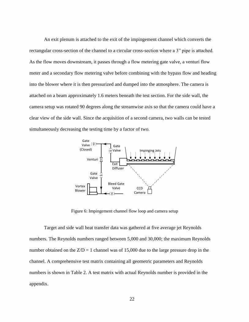
An exit plenum is attached to the exit of the impingement channel which converts the
rectangular cross-section of the channel to a circular cross-section where a 3” pipe is attached.
As the flow moves downstream, it passes through a flow metering gate valve, a venturi flow
meter and a secondary flow metering valve before combining with the bypass flow and heading
into the blower where it is then pressurized and dumped into the atmosphere. The camera is
attached on a beam approximately 1.6 meters beneath the test section. For the side wall, the
camera setup was rotated 90 degrees along the streamwise axis so that the camera could have a
clear view of the side wall. Since the acquisition of a second camera, two walls can be tested
simultaneously decreasing the testing time by a factor of two.
Bleed Gate Valve
Gate Valve
Venturi
Vortex Blower
Gate Valve
(Closed)Gate Valve
CCD Camera
Exit Diffuser
Impinging Jets
Figure 6: Impingement channel flow loop and camera setup
Target and side wall heat transfer data was gathered at five average jet Reynolds
numbers. The Reynolds numbers ranged between 5,000 and 30,000; the maximum Reynolds
number obtained on the Z/D = 1 channel was of 15,000 due to the large pressure drop in the
channel. A comprehensive test matrix containing all geometric parameters and Reynolds
numbers is shown in Table 2. A test matrix with actual Reynolds number is provided in the
appendix.

23
Table 2: Test Matrix
X/D Y/D Z/D Reynolds number
5 4
1
5,000
7,500
10,000
12,500
15,000
2
10,000
15,000
20,000
25,000
30,000
3
10,000
15,000
20,000
25,000
30,000
5
10,000
15,000
20,000
25,000
30,000
7
10,000
15,000
20,000
25,000
30,000
9
10,000
15,000
20,000
25,000
30,000

24
Temperature sensitive paint, or TSP, is used to gather temperature data on the surface of
the test section. The TSP is purchased from ISSI in 500 ml cans. The lab were the experiments
were performed has a long history of TSP usage; hence, multiple calibrations exist. In order to
ensure the use of the correct calibration a test piece was painted with the TSP can that is used to
paint all side and target walls. The test piece was surrounded by ROHACELL isolative foam in
order to ensure no lateral heat transfer. The painted test piece was attached to a copper block
with the use of double sided Kapton tape. The copper block was attached to a thermoelectric
heater with copper tape as well as heat sink thermal paste in order to reduce contact resistance. A
computer heat sink was attached to the cold side of the thermoelectric heater in order to
maximize heat transfer. A US sensor thermistor was embedded into the copper block covered
with thermal paste in order to ensure proper contact and a correct temperature measurement.
Figure 7 shows a diagram of the TSP calibration setup.

25
Figure 7: Temperature sensitive paint calibration setup
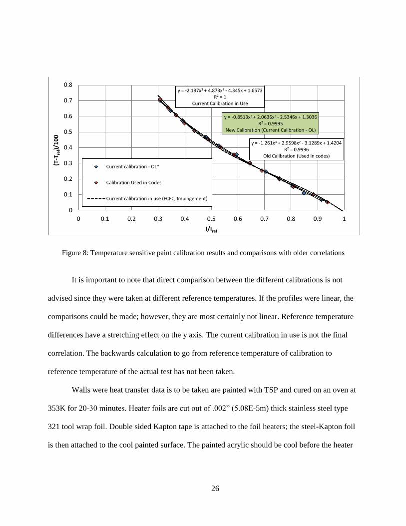
Calibration was done at multiple temperatures; thirty images were taken and averaged
alongside their respective thermistor resistance measurement. Only the center region of the TSP
was used to collect the area averaged intensity of each image set. Thermistor resistances were
converted into temperatures with the use of the correlations provided by the manufacturer. Image
intensity ratios are then plotted versus temperature ratios and a third order polynomial curve was
fitted to the data. Figure 8 shows the strong agreement between the current calibration and the
legacy calibration used in the codes. The small deviation between all calibrations provides a
sense of robustness of the TSP as its calibration varies very slightly with time.
26
Figure 8: Temperature sensitive paint calibration results and comparisons with older correlations
It is important to note that direct comparison between the different calibrations is not
advised since they were taken at different reference temperatures. If the profiles were linear, the
comparisons could be made; however, they are most certainly not linear. Reference temperature
differences have a stretching effect on the y axis. The current calibration in use is not the final
correlation. The backwards calculation to go from reference temperature of calibration to
reference temperature of the actual test has not been taken.
Walls were heat transfer data is to be taken are painted with TSP and cured on an oven at
353K for 20-30 minutes. Heater foils are cut out of .002” (5.08E-5m) thick stainless steel type
321 tool wrap foil. Double sided Kapton tape is attached to the foil heaters; the steel-Kapton foil
is then attached to the cool painted surface. The painted acrylic should be cool before the heater
y = -0.8513x3 + 2.0636x2 - 2.5346x + 1.3036 R² = 0.9995
New Calibration (Current Calibration - OL)
y = -1.261x3 + 2.9598x2 - 3.1289x + 1.4204 R² = 0.9996
Old Calibration (Used in codes)
y = -2.197x3 + 4.873x2 - 4.345x + 1.6573 R² = 1
Current Calibration in Use
0
0.1
0.2
0.3
0.4
0.5
0.6
0.7
0.8
0 0.1 0.2 0.3 0.4 0.5 0.6 0.7 0.8 0.9 1
(T-T
ref)
/10
0
I/Iref
Current calibration - OL*
Calibration Used in Codes
Current calibration in use (FCFC, Impingement)
27
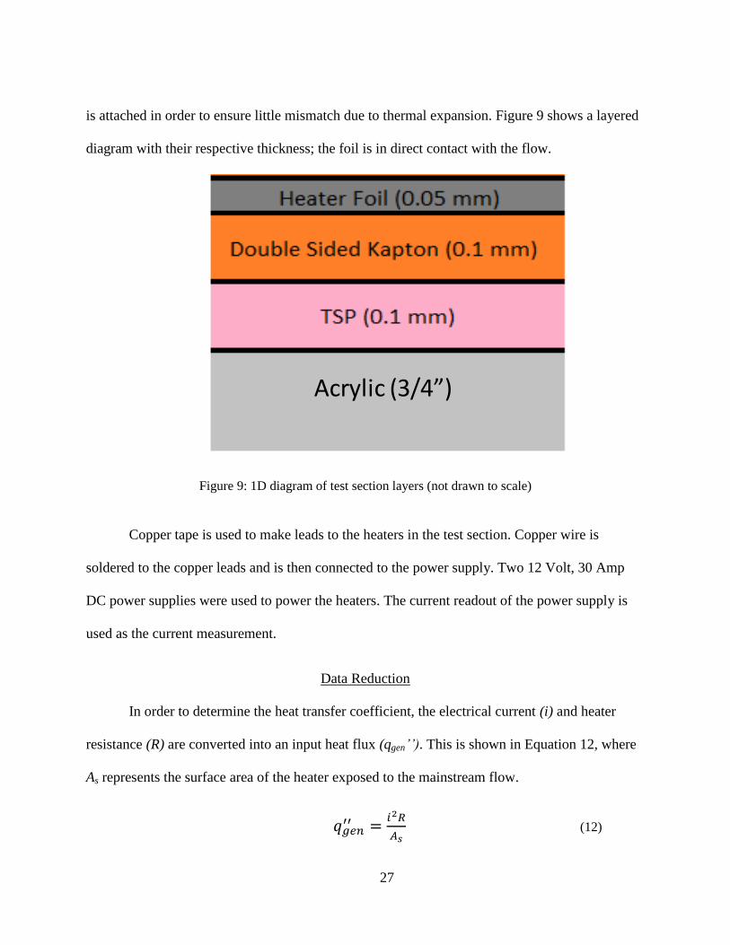
is attached in order to ensure little mismatch due to thermal expansion. Figure 9 shows a layered
diagram with their respective thickness; the foil is in direct contact with the flow.
Figure 9: 1D diagram of test section layers (not drawn to scale)
Copper tape is used to make leads to the heaters in the test section. Copper wire is
soldered to the copper leads and is then connected to the power supply. Two 12 Volt, 30 Amp
DC power supplies were used to power the heaters. The current readout of the power supply is
used as the current measurement.
Data Reduction
In order to determine the heat transfer coefficient, the electrical current (i) and heater
resistance (R) are converted into an input heat flux (qgen’’). This is shown in Equation 12, where
As represents the surface area of the heater exposed to the mainstream flow.
(12)
Acrylic (3/4”)
28
The heater resistance is calculated using the resistivity (ρel) of stainless steel and the
dimensions of the heater. The length (l) is measured in the stream direction, x, while the width
(w) is measured in the span direction, y. The thickness (t) is the thickness of the stainless steel
foil, measured in the wall normal direction, z.
(13)
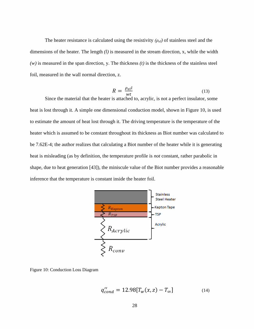
Since the material that the heater is attached to, acrylic, is not a perfect insulator, some
heat is lost through it. A simple one dimensional conduction model, shown in Figure 10, is used
to estimate the amount of heat lost through it. The driving temperature is the temperature of the
heater which is assumed to be constant throughout its thickness as Biot number was calculated to
be 7.62E-4; the author realizes that calculating a Biot number of the heater while it is generating
heat is misleading (as by definition, the temperature profile is not constant, rather parabolic in
shape, due to heat generation [43]), the miniscule value of the Biot number provides a reasonable
inference that the temperature is constant inside the heater foil.
Figure 10: Conduction Loss Diagram
(14)

29
The analytical model lacks the contact resistances between the interfaces of the Kapton,
TSP and the heaters; the model also assumes constant properties of the materials as a function of
temperature as well as the estimation of the backside heat transfer coefficient; due to all these
inaccuracies, a heat loss test was setup on the actual test section to more accurately gauge the
backside heat loss. The channel was filled with fiberglass insulation to ensure all the heat was
lost through the acrylic. Four points were taken at different temperature ranges. The resulting
curve is shown in Figure 11
Figure 11: Heat loss results and correlation
The corresponding heat loss equation then varies slightly to become:
(15)
Normal test heat fluxes ranged between 11,000 and 4,000 W/m2 with area averaged
temperature difference between the TSP and the atmosphere at 35 and 30 K respectively;
therefore, typical heat loss was near 5% of the heat generated. Since there is higher fidelity on
the correlation acquired by running the heat loss test, it will be used instead of the analytical
model to calculate the heat transfer.
q" = 15.886∙ΔT R² = 0.9998
0
100
200
300
400
500
600
700
800
900
0 10 20 30 40 50 60
He
at F
lux
(W/m
2 )
Temperature Difference (oC)

30
Pressure measurements were taken from the taps installed on the side wall of the channel
with a handheld manometer. The pressure taps were located in between jet rows. Figure 12
shows a sample of the pressure profile acquired from the test. Each point is an average of a set of
30 measurements.
Figure 12: Sample Pressure Profile
This pressure data was then converted into absolute pressure in Pascals. The pressure
ratio across the jet plate was then calculated, followed by the Mach number. The highest jet
Mach number was calculated to be 0.19 at a pressure ratio of 1.027. Since the highest Mach
number doesn’t exceed 0.3, the flow is in the incompressible range. The jet velocity was then
calculated using:.
(16)
(17)
-12
-10
-8
-6
-4
-2
0
0 5 10 15 20
Pga
uge
(in
H2O
)
Jet Number

31
Each individual jet velocity was then multiplied by the array-average discharge
coefficient, Cd, to acquire an actual jet velocity. The jet mass flux ratio was then obtained using.
(18)
Channel mass flux was calculated using equation 19; equation 20 was used to calculate
channel to jet mass flux ratio.
(19)
(20)
The calculated mass flux ratios are compared with the analytical model provided by
Florschuetz; Local jet mass flux to average jet mass flux ratio is given by:
(21)
Crossflow-to-jet mass flux ratio is given by:
(22)
where β is given by:
(23)

32
Lateral Conduction Estimation
Lateral conduction through the heater is believed to be significant due to the nature of the
heat transfer profiles. Large temperature gradients are encountered at low x/D between the cool
stagnation region of the jet and the hot region between impinging jets. One dimensional lateral
conduction calculations were done on the steel heater; the Kapton tape, paint and acrylic were
omitted due to their thermal conductivities being an order of magnitude smaller than that of the
steel; this assumption, as shown further ahead, is proven to be valid for all heat transfer profiles
shown in this study. In order to do the calculation, the Nusselt number profile with the highest
spatial Nusselt number inequality was used. Several profiles were tested to find the one with the
highest Nusselt number gradient; Z/D=2 target wall heat transfer profile at Rejavg=30,000 was
found to have the largest temperature gradient. A two dimensional conduction model was used to
calculate the heat flux in the lateral direction though the steel foil compared to the heat flux in
the wall normal direction driven by convection.
Figure 13 shows the results of the calculations; the blue dotted line shows the net lateral
heat flux though the steel foil. The slope is seen to reach zero at the peak of Nusselt number due
to the gradient being zero; as x moves away from the peak, the lateral conduction increases in
magnitude. The red curve shows the wall normal heat flux. It is seen that the lateral conduction is
two orders of magnitude less important than the wall normal heat flux. More importantly, the
variation in wall normal heat flux is seen to be very monotonous throughout the stagnation
region, reassuring the assumption of constant flux throughout the domain. A complete set of
calculations can be found on the appendix

33
Figure 13: Lateral Conduction Estimates
0.14 0.15 0.16 0.171 10
5
1 104
1 103
0.01
qconv x( )
qnet x( )
x x

34
CHAPTER FIVE: EXPERIMENTAL UNCERTAINTY
Experimental uncertainties were quantified using the methods described in Figliola and
Beasly [44]. Five runs were setup using the Z/D=3 channel testing target wall heat transfer to
quantify the precision uncertainty of Nusselt number as well as Reynolds number. The bias error
for each measurand was gauged by reading the manuals of the respective instruments.
A table showing absolute uncertainties for Nusselt and Reynolds number are shown
below in Table 3 and Table 4, respectively. The measurands for Nusselt number are the current,
electrical resistivity of the steel, width and thickness of the heater, reference and test intensity, jet
diameter as well as plenum and reference temperatures. The measurands for Reynolds number
are the static pressure at the Venturi, atmospheric pressure, Venturi temperature, Delta pressure
in the Venturi and jet diameter.
Table 3: Absolute and Relative Nusselt Number Uncertainties
Nusselt Number Uncertainty
Measurand Bias Precision
Current 5.263 0.904
Electrical Resistivity 0.513 0
Width of Heater 0.125 0.293
Thickness of Heater 0.185 0
Intensity 0.015 5
Reference Intensity 0.011 9.789
Plenum Temperature 3.257 1.647
Reference Temperature 3.257 1.044
Hole Diameter 0.239 0.379
Individual Totals 7.02 11.21
Total Uncertainty 13.23
Relative Uncertainty 18.90%

35
Table 4: Absolute and Relative Reynolds Number Uncertainties
Reynolds Number Uncertainty
Measurand Bias Precision
Venturi Static Pressure 57.904 1.206
Atmospheric Pressure 0.56 15.123
Venturi Temperature 36.484 10.426
Delta Pressure 2532 210.288
Diameter 79.689 6.00E-12
Individual Totals 2534.18 211.09
Total Uncertainty 2542.95
Relative Uncertainty 10.91%
In order to facilitate the understanding of the major sources of uncertainty, the bias and
precision absolute uncertainties are plotted for both Nusselt and Reynolds number. They are
shown in Figure 14 and Figure 15, respectively.
Figure 14: Absolute Uncertainties of Nusselt Number
0 2 4 6 8 10 12
Current
Electrical Resistivity
Width of Heater
Thickness of Heater
Intensity
Reference Intensity
Plenum Temperature
Reference Temperature
Hole Diameter
Bias
Precision

36
Figure 15: Absolute Uncertainties of Reynolds Number
The largest source of uncertainty for the Nusselt number comes from the precision in
intensities due to the repeated use of the same paint in all the precision runs. Electrical current
plays a major role in the bias followed by the reference and plenum temperatures; acquiring
better instrumentation for the temperature measurements would be advisable since it provides
large drops in uncertainty with little cost. The precision uncertainty for the Reynolds number is
almost non-existent. The largest source of uncertainty for Reynolds number is the DP
measurement across the Venturi. Using multiple manometers to measure pressures in their
optimum range would be advisable in the future. Two different manometers were used for these
experiments; the worst of the two was used for the bias uncertainty.
0 500 1000 1500 2000 2500 3000
Venturi Static Pressure
Atmospheric Pressure
Ventiru Temperature
Delta Pressure
Diameter
Bias
Precision

37
CHAPTER SIX: FLOW RESULTS
Using the aforementioned equations, mass flux ratio distributions were calculated and
compared with the analytical models provided by Florschuetz, et al. [19] Channel mass flux to
jet mass flux ratio distribution and their comparisons to the analytical models are shown in
Figure 16. The model and local data match at large channel heights; however, as the channels get
smaller, friction causes a significant pressure drop as a function of streamwise distance causing
the model and experimental data to deviate. Exit effects may also cause misleading pressure
measurements on the downstream-most pressure tap.
Figure 16: Channel mass flux to jet mass flux ratio distribution
0
0.2
0.4
0.6
0.8
1
1.2
0 10 20 30 40 50 60 70 80
Gc/
Gj
x/D
Z/D=1 Prediction Z/D=1 Z/D=2 Prediction Z/D=2
Z/D=3 Prediction Z/D=3 Z/D=5 Prediction Z/D=5
Z/D=7 Prediction Z/D=7 Z/D=9 Prediction Z/D=9

38
Local jet mass flux to average jet mass flux is also calculated and compared to the
analytical model; the results are shown in Figure 17. The mass flux ratio indicate the deviation of
the local jet Reynolds number from the average jet Reynolds number; that is, for the Z/D = 1
case, the first jet approximately has a Reynolds number 65% lower than the average jet Reynolds
number. The variation in local jet Reynolds number is large for low impingement heights with
the local jet Reynolds number varying by an order of magnitude between the first and last jet. As
the channel height increases, the jet Reynolds number profile flattens as the pressure drop in the
larger channels is smaller than the one on the smaller channels. As previously described, large
pressure drop inside the channels with small impingement height is believed to be the source of
discrepancy between the analytical model and the experimental data.
Figure 17: Local jet mass flux to average jet mass flux ratio and comparisons to analytical models
0
0.5
1
1.5
2
2.5
3
3.5
0 10 20 30 40 50 60 70 80
Gj/
Gja
vg
x/D
Z/D=1 Prediction Z/D=1
Z/D=2 Prediction Z/D=2
Z/D=3 Prediction Z/D=3
Z/D=5 Prediction Z/D=5
Z/D=7 Prediction Z/D=7
Z/D=9 Prediction Z/D=9

39
CHAPTER SEVEN: HEAT TRANSFER RESULTS
Smooth Channel Validation
Heat transfer data was collected on two walls of the impingement channel as explained
previously. A validation run used to compare the results of the current test setup with heat
transfer results that are widely known was done. The Z/D = 3 channel was setup by blocking all
the hole exits on the flow side of the jet play with clear smooth packing tape. On the plenum
side, the jet plate was sealed with aluminum tape to ensure no leakage flow though the 15 jets.
The front end cap was removed; a trip wire was placed near the target wall to trip the flow in
order for it to develop faster. The data was gathered using the target wall at two Reynolds
numbers based off of hydraulic diameter of the channel. The length of the channel was close to
22 hydraulic diameters ensuring a fully developed hydrodynamic and thermal boundary layer.
The span averages of the validation runs are shown in Figure 18. The profiles are normalized by
their corresponding Dittus-Boelter correlation [43]. The Nusselt number profile starts high when
both hydrodynamic and thermal boundary layers are developing. As the streamwise distance
decreases, both profiles are seen to converge near unity signifying a successful validation of the
channel with respect to the well-accepted Dittus-Boelter correlation. A validation attempt using
the Z/D=1 channel was done with the results matching well in the area averaged basis; however,
due to the Z/D=1 channel having an aspect ratio of 4, the local profiles exhibited local non
uniformities at the entrance of the channel possibly due to secondary flows. It was then decided
to validate with a channel with an aspect ratio as close as possible to 1 which lead to the
choosing of the Z/D=3 channel.

40
Figure 18: Smooth Channel Validation
Heat Transfer Results
Now with the experimental setup validated, results for the target wall and side walls are
shown for some Reynolds numbers and all channel heights. The heat transfer profiles of all walls
and channels at all Reynolds numbers are shown in the appendix; for the sake of brevity, only
comparisons are shown and described in this chapter. Figure 20 and Figure 20 show the target
wall Nusselt number profiles at average jet Reynolds number of 10,000 and 15,000 respectively.
The Z/D=1 profile features increasing heat transfer as a function of streamwise distance, x. Local
maxima are seen directly underneath the jets generated due to the jet impinging on the surface.
The Nusselt number profile for the Z/D = 2 channel exhibits the most uniform heat transfer
outline out of all channels; although maxima due to jet impingement are visible, the Nusselt
number does not seems to be a function of the streamwise location. As channel heights increases,
the stagnation region Nusselt number decreases for the first few jets and quickly decreases as a
0
0.2
0.4
0.6
0.8
1
1.2
1.4
1.6
1.8
2
0 5 10 15 20 25
Nu
/Nu
DB
x/Dh
ReDh = 83,000
ReDh = 97,000

41
function of streamwise distance. One feature seen in the target wall profiles for both Reynolds
number is the dominance of the second – and sometimes the third – jet over the first one. The
Florschuetz et al. correlation does not predict this behavior. It may be caused by transient effects
where the crossflow from the first jet may be shedding vortices that affect the behavior of the
downstream jets by forcing them to deflect from their centerline in a periodic fashion allowing it
to cool a larger area. It would be advisable to run a URANS simulation of the first 5 jets to see if
there are transient flow fields caused by the upstream jet.
The downstream shift of the jets due to crossflow is seen in the local target wall profiles.
The Z/D = 2 channel only contains 14 distinct peaks visible implying that the 15th
jet has been
deflected by the crossflow downstream by at least 3 diameters; this downstream shift is expected
as the mass flux ratio between the channel and the jet reaches a value near Gc/Gj=0.8 which
implies the crossflow is coming in with a velocity close to the velocity of the jet. The equivalent
blowing ratio analogy is that the jet has a blowing ratio of M=1.25 which, as seen in the film
cooling literature allows for the jet to liftoff from the surface but is quickly deflected
downstream.
The shapes of the Nusselt number distribution caused by the first jet is circular of Z/D= 2,
3, 5, 7, and 9. As crossflow builds up, the jets start being deflected downstream causing their
shapes to morph into a parabolic shape that is sharp at the centerline and blunt on the sides. The
change of shape is due to the wall jet of the upstream jet moving downstream creating an up
wash similar to a hydraulic jump; the upstream wall jet moves above the local wall jet generating
the detrimental crossflow. Local minima and maxima are not visible far downstream of the Z/D
= 7 and 9 channels due to the jets not having enough momentum to reach the target wall; it is
presumed that the heat transfer in this regions is dominated by the crossflow.

42
Figure 19: Target Wall Comparison at Rejavg=10,000
Figure 20: Target Wall Comparison at Rejavg=15,000
Side wall Nusselt number contours are shown in Figure 21 and Figure 22 for Rejavg =
10,000 and Rejavg = 15,000 respectively. The stagnation regions of the wall jets are visible at low
z/D. Similarly to its respective target wall heat transfer profile, the Z/D=1 side wall Nusselt
number profile shows increasing Nusselt number as a function of streamwise distance. The side
wall profiles show less distinct maxima than their respective target wall; this may be attributed to
the fact that the wall jets have to travel a distance of two diameters in either direction before
impinging on the side wall. As stated previously, the shapes of the Nusselt number profiles
changes as a function of streamwise location and channel height; the deflection of the wall jet

43
downstream prevents it from reaching the side wall. For the Z/D = 2 channel, as streamwise
distance increases, the Nusselt number is also seen to increase maintaining the trend seen in the
Z/D = 2 target wall of it having the most uniform Nusselt number profile.
One notable difference in side wall Nusselt number profile as a function of channel
heights comes from the deflection of the jets downstream with increased crossflow; as stated
previously, the downstream deflection in Nusselt number maxima can be seen having a greater
effect on the side wall than on the target wall profiles. At low channel heights, the local maxima
occurs at low z/D (near the target wall). The trend holds accurate for the first 4 or 5 jets at all
channel heights. The peak starts shifting to a higher z/D for the tall channels, Z/D = 5, 7 and 9.
The shift of the maxima to locations away from the target wall is due to the crossflow not
allowing the jet to reach the target wall; instead, the jet gets deflected downstream diffusing, and
possibly wobbling from side to side due to vortex shedding of the upstream jets causing it to only
alter the side wall heat transfer; the maxima are seen at an x/D=3.5 for the Z/D = 7 channel and
at an x/D=4.5 for the Z/D = 9
Figure 21: Side Wall Comparison at Rejavg=10,000

44
Figure 22: Side Wall Comparison at Rejavg=15,000
In order to better understand the heat transfer profiles, laterally averaged plots of Nusselt
number are shown only for Rejavg = 15,000 in Figure 23 for all target walls and Figure 24 for all
side walls. Demonstrating the points made previously, the Z/D=1 profile is seen to increase as a
function of streamwise location, the Z/D=2 lateral average confirms the fact that it, alongside the
Z/D=3 channel, is very uniform in the streamwise direction. The profiles of the Z/D= 5, 7 and 9
channels seem to decrease monotonically as a function of the channel height. Comparisons
between the target and side walls show the difference in downstream shift of peaks in Nusselt
number. From a systems point of view, the area averaged Nusselt number does not vary
significantly for any channel height; however, the Z/D = 2 and 3 channel seem to provide the
highest cooling capability at a relatively low (compared to Z/D = 1) pressure loss.

45
Figure 23: Target Wall Nusselt number Comparisons at Rejavg=15,000
Figure 24: Side Wall Nusselt number Comparisons at Rejavg=15,000
0
20
40
60
80
100
120
0 10 20 30 40 50 60 70 80
Nu
x/D
Z/D=1 - Re=14,500 Z/D=2 - Re=15,000
Z/D=3 - Re=15,000 Z/D=5 - Re=15,000
Z/D=7 - Re=15,000 Z/D=9 - Re=15,000
Jet Locations
0
10
20
30
40
50
60
70
0 10 20 30 40 50 60 70 80
Nu
x/D
Z/D=1 - Re=14,500 Z/D=2 - Re=15,000
Z/D=3 - Re=15,000 Z/D=5 - Re=15,000
Z/D=7 - Re=15,000 Z/D=9 - Re=15,000
Jet Locations

46
One of the major focuses of this project is to understand the interaction between the
target and side wall heat transfer profiles. Isometric views were generated by placing the side
wall Nusselt number profiles in the vertical position and the target wall profiles in the horizontal
position for all channel heights; due to the target and side walls being run at the same time, the
corresponding Reynolds numbers are identical for both walls shown at a single channel height.
The isometric view of Rejavg = 10,000 is shown in Figure 25 while the one for Rejavg =
15,000 is shown in Figure 26. The profiles seen here are identical to the ones seen in figures
Figure 206, Figure 20, Figure 21, and Figure 22 rearranged in order to get a better feel of the
interaction between the two walls.
At low impingement height, the high Nusselt number regions of the side wall are seen to
match directly with the ones seen on the target wall for the first couple of jets; as the downstream
distance increases, the side wall peaks are seen to be shifting downstream with respect to the
corresponding peak in target wall Nusselt number. This direct comparison shows the impact of
the crossflow by forcing through both sides of the channel and deflecting the wall jet
downstream. Similar to the description by Florschuetz et at. [18] explaining that the negative
effect of the crossflow is a combination of mass flux ratio, Gc/Gj, and channel height, Z/D; it is
seen that the downstream shift of the side wall is also proportional to the mass flux ratio and
channel height. Additional differences are the shift of the maxima on the tall side walls away
from the target wall at middle streamwise locations.

47
Figure 25: Isometric View of all Channels at Rejavg=10,000
Figure 26: Isometric View of all Channels at Rejavg=15,000

48
CHAPTER EIGHT: HEAT TRANSFER DATA ANALYSIS
Nusselt Number Dependence of Reynolds number
Reynolds number dependence of all channels was studied. The 15 points of pitch
averaged Nusselt number were averaged to generate an area average for each wall at every single
Reynolds number. It is seen in the literature that Nusselt number trends proportional to Reynolds
number raised to a power “m”. Taking a logarithmic of both quantities, Nusselt and Reynolds
number, and plotting the five resulting points alongside a linear fit provides the Reynolds
number exponent “m” as the slope of the linear regression. This process was done for all channel
heights on both the target and side walls. Table 5 shows the values of the “m” coefficients for all
twelve cases.
Table 5: Nusselt Number Dependence on Reynolds Number
Target Wall Side Wall Average
Z/D=1 0.847 0.910 0.88
Z/D=2 0.906 0.879 0.89
Z/D=3 0.780 0.836 0.81
Z/D=5 0.631 0.750 0.69
Z/D=7 0.869 0.788 0.83
Z/D=9 0.785 0.760 0.77
The non-monotonic variation of Reynolds number exponents throughout the domain does
not lend the data to be collapsed by any function of Reynolds number exponent versus channel
height function as the one given by Florschuetz et al. [18]. Throughout the first four channel
heights, Z/D = 1, 2, 3, and 5, the values seem to be decreasing as expected by the Florschuetz et
al. correlation; however, once Z/D = 7 and 9 are considered, the trend collapses. The cause of
this anomaly is believed to originate due the combination of uncertainty from Reynolds Number
and Nusselt number combining leading the uncertainty of the Reynolds number coefficient to be
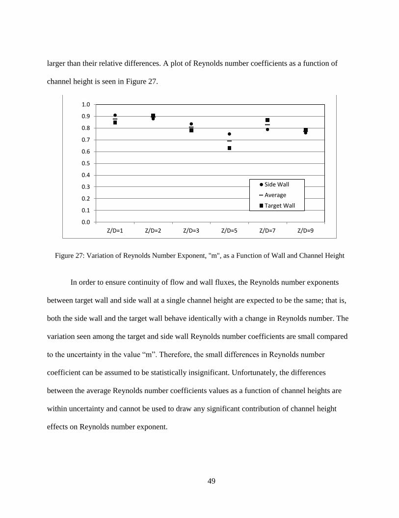
49
larger than their relative differences. A plot of Reynolds number coefficients as a function of
channel height is seen in Figure 27.
Figure 27: Variation of Reynolds Number Exponent, "m", as a Function of Wall and Channel Height
In order to ensure continuity of flow and wall fluxes, the Reynolds number exponents
between target wall and side wall at a single channel height are expected to be the same; that is,
both the side wall and the target wall behave identically with a change in Reynolds number. The
variation seen among the target and side wall Reynolds number coefficients are small compared
to the uncertainty in the value “m”. Therefore, the small differences in Reynolds number
coefficient can be assumed to be statistically insignificant. Unfortunately, the differences
between the average Reynolds number coefficients values as a function of channel heights are
within uncertainty and cannot be used to draw any significant contribution of channel height
effects on Reynolds number exponent.
0.0
0.1
0.2
0.3
0.4
0.5
0.6
0.7
0.8
0.9
1.0
Z/D=1 Z/D=2 Z/D=3 Z/D=5 Z/D=7 Z/D=9
Side Wall
Average
Target Wall

50
Total Heat Transfer Contribution
In order to see which channel provides the maximum amount of heat transfer, the area
averaged Nusselt number at Rejavg=10,000 and 15,000 were multiplied with their respective
width. For example, all target wall area averaged Nusselt numbers were multiplied by Yc/D=4,
all side walls were multiplied by their respective non dimensional heights, Z/D, and by a factor
of two signifying the contributions from both side walls. A table was generated with the
contributions from target and side walls as well as their sum being shown at the two Reynolds
numbers. The results are shown in Table 6.
Table 6: Total Channel Heat Transfer
Rejavg=10,000 Rejavg=15,000
Target Wall Contribution
Side Wall Contribution Total
Target Wall Contribution
Side Wall Contribution Total
Z/D=1 137 44 180 199 75 274
Z/D=2 166 125 291 223 164 387
Z/D=3 145 150 296 200 221 420
Z/D=5 135 216 350 154 286 440
Z/D=7 91 269 360 125 365 490
Z/D=9 76 295 371 102 395 496
In order to get a better feeling of the specific contributions from target and side walls on
the total heat transfer of the channel, they were plotted as a function of channel height for both
Reynolds numbers; Figure 28 shows the channel heat transfer for a Reynolds number of 10,000
while Figure 29 shows it for a Reynolds number of 15,000. It can be seen that the trends do not
vary with Reynolds number. The maximum overall heat transfer rate is achieved by the Z/D=9
channel due to the large area that the heat has the ability to travel through. The designer must
choose a balance between target wall heat transfer versus increasing the side wall heat transfer
area. It seems that a Z/D=3 supports the highest target wall and side wall heat transfer

51
coefficients. Other parameters are also to be taken into account such as availability of space and
the minimum acceptable target wall heat transfer.
Figure 28: Contributions of Target and Side Walls on Overall Channel Heat Transfer for Rejavg=10,000
0
50
100
150
200
250
300
350
400
Z/D=1 Z/D=2 Z/D=3 Z/D=5 Z/D=7 Z/D=9
NU
sse
lt N
um
be
r *
Ap
plie
d W
idth
Target Wall Contribution
Side Wall Contribution
Total

52
Figure 29: Contributions of Target and Side Walls on Overall Channel Heat Transfer for Rejavg=15,000
Comparisons with Florschuetz et al. [18] Correlation
Using the correlation provided by Florschuetz et at. [18], two channel heights were
compared at two Reynolds numbers each. The channel heights compared were Z/D = 2 which
lies well within the test matrix of Florschuetz et al. and Z/D=3 which lies at one extreme end of
the test matrix. The results are shown in Figure 30 for Z/D=2 channel and in Figure 31 for the
Z/D=3 channel.
The results of the Z/D=2 channel are seen to agree well with the Florschuetz et al.
correlation; the correlation predicts a slight decrease in heat transfer due to crossflow followed
by an increase in heat transfer due to an increase of jet mass flux as a function of streamwise
location previously described with the use of Figure 17.
0
100
200
300
400
500
600
Z/D=1 Z/D=2 Z/D=3 Z/D=5 Z/D=7 Z/D=9
NU
sse
lt N
um
be
r *
Ap
plie
d W
idth
Target Wall Contribution
Side Wall Contribution
Total

53
Figure 30: Z/D = 2 Nusselt Number Profile Comparisons with Florschuetz et al.
The Z/D = 3 results do not match as well as the ones for the Z/D = 2 channel. The
discrepancy may be due to the Florschuetz correlation not being valid at one of the corners of the
Florschuetz matrix (Z/D = 5, Y/D = 4, Z/D = 3). The results; however, show an interesting aspect
of the profile that is predicted by the correlation which is the positive concavity of the Nusselt
number profile; as Gc/Gj increases, there comes a point where the crossflow starts dominating
the heat transfer inside the channel and its effects switch from being detrimental to the overall
heat transfer at low x/D to an increase in heat transfer due to channel flow similar to the one
predicted by the Dittus-Boelter correlation.
The area averaged values of the Florschuetz correlation compared to the area averaged
values of the current data lie within experimental uncertainty of both the correlation and the
current data. Having the uncertainty estimates being significant compared to the magnitude of
the difference between the prediction and the actual values as well as the knowledge that the
0
10
20
30
40
50
60
70
80
90
100
0 10 20 30 40 50 60 70 80
Nu
x/D
Z/D=2 - Re=15,000 Z/D=2 - Re=19,900 Florschuetz Prediction Re = 15,000 Florschuetz Prediction Re = 19,900 Jet Locations
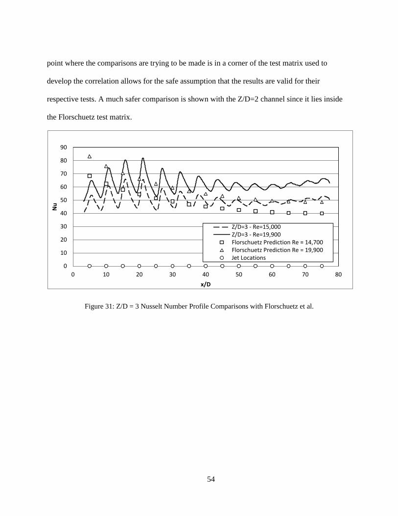
54
point where the comparisons are trying to be made is in a corner of the test matrix used to
develop the correlation allows for the safe assumption that the results are valid for their
respective tests. A much safer comparison is shown with the Z/D=2 channel since it lies inside
the Florschuetz test matrix.
Figure 31: Z/D = 3 Nusselt Number Profile Comparisons with Florschuetz et al.
0
10
20
30
40
50
60
70
80
90
0 10 20 30 40 50 60 70 80
Nu
x/D
Z/D=3 - Re=15,000 Z/D=3 - Re=19,900 Florschuetz Prediction Re = 14,700 Florschuetz Prediction Re = 19,900 Jet Locations
55
CHAPTER NINE: CONCLUSIONS
The work by Ricklick [45] has been continued to fully understand the effect of channel
height on target wall as well as side wall Nusselt number. The research involves the heat transfer
characterization of six inline impingement channels at channel heights of Z/D = 1, 2, 3, 5, 7, and
9. A single streamwise jet spacing of X/D = 5 and lateral spacing of Y/D = 4 was studied. It is
shown that the target and side walls interact to generate large heat transfer profiles at the lower
height of the side walls. Results also show dependencies of the downstream shift in Nusselt
number on channel height and mass flux ratios as previously seen by Florschuetz et al. [17]
The impact of side walls were seen to be significant when total channel heat transfer was
calculated; at low impingement heights, the side walls, due to their small size, do not display a
significant amount of heat transfer capability; however, as the channel height increase, the effect
of side walls on overall heat transfer increases. At Z/D=3 the two side walls have the same heat
transfer capacity as the single target wall; as Z/D increases, although the area averaged Nusselt
number drops, the overall heat transfer capability increases due to the larger area. At Z/D=1, both
side walls accounted for a mere 24% of the overall heat transfer of the channel; at a Z/D=3, the
side walls provided a total of 50% of the heat transfer; as the channel height is increased to Z/D
= 9 the amount of heat transfer provided by the side walls increased 80% of the heat transfer
capacity of the channel. The previous results symbolize the importance of the inclusion of side
wall heat transfer to a confined impingement channel.

56
APPENDIX A: NUSSELT NUMBER PROFILES

57
Figure 32: Z/D=1 Target Wall Nusselt number Profiles at Multiple Reynolds Numbers
Figure 33: Z/D=2 Target Wall Nusselt number Profiles at Multiple Reynolds Numbers
Figure 34: Z/D=3 Target Wall Nusselt number Profiles at Multiple Reynolds Numbers
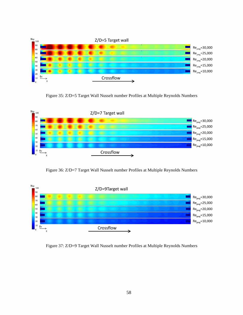
58
Figure 35: Z/D=5 Target Wall Nusselt number Profiles at Multiple Reynolds Numbers
Figure 36: Z/D=7 Target Wall Nusselt number Profiles at Multiple Reynolds Numbers
Figure 37: Z/D=9 Target Wall Nusselt number Profiles at Multiple Reynolds Numbers
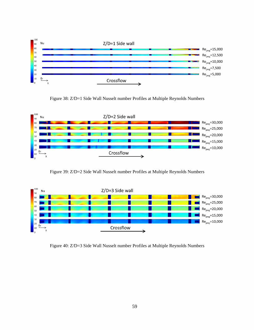
59
Figure 38: Z/D=1 Side Wall Nusselt number Profiles at Multiple Reynolds Numbers
Figure 39: Z/D=2 Side Wall Nusselt number Profiles at Multiple Reynolds Numbers
Figure 40: Z/D=3 Side Wall Nusselt number Profiles at Multiple Reynolds Numbers

60
Figure 41: Z/D=5 Side Wall Nusselt number Profiles at Multiple Reynolds Numbers
Figure 42: Z/D=7 Side Wall Nusselt number Profiles at Multiple Reynolds Numbers

61
Figure 43: Z/D=9 Side Wall Nusselt number Profiles at Multiple Reynolds Numbers

62
APPENDIX B: SPAN AVERAGED NUSSELT NUMBER DATA

63
Figure 44: Target Wall Laterally Averaged Nusselt Number for Z/D=1
Figure 45: Side Wall Laterally Averaged Nusselt Number for Z/D=1
0
20
40
60
80
100
120
0 10 20 30 40 50 60 70 80
Nu
x/D
Z/D=1 - Re=4,900 Average Nu - Re=4,900
Z/D=1 - Re=14,500 Average Nu - Re=14,500
Z/D=1 - Re=12,500 Average Nu - Re=12,500
Z/D=1 - Re=10,100 Average Nu - Re=10,100
Z/D=1 - Re=7,400 Average Nu - Re=7,400
Jet Locations
0
10
20
30
40
50
60
70
80
0 10 20 30 40 50 60 70 80
Nu
x/D
Z/D=1 - Re=14,500 Average Nu - Re=14,500
Z/D=1 - Re=12,500 Average Nu - Re=12,500
Z/D=1 - Re=10,100 Average Nu - Re=10,100
Z/D=1 - Re=7,400 Average Nu - Re=7,400
Z/D=1 - Re=4,900 Average Nu - Re=4,900
Jet Locations

64
Figure 46: Target Wall Laterally Averaged Nusselt Number for Z/D=2
Figure 47: Wall Laterally Averaged Nusselt Number for Z/D=2
0
20
40
60
80
100
120
140
160
180
0 10 20 30 40 50 60 70 80
Nu
x/D
Z/D=2 - Re=10,000 Average Nu - Re=10,000
Z/D=2 - Re=29,400 Average Nu - Re=29,400
Z/D=2 - Re=24,900 Average Nu - Re=24,900
Z/D=2 - Re=19,900 Average Nu - Re=19,900
Z/D=2 - Re=15,000 Average Nu - Re=15,000
Jet Locations
0
20
40
60
80
100
120
140
0 10 20 30 40 50 60 70 80
Nu
x/D
Z/D=2 - Re=29,400 Average Nu - Re=29,400 Z/D=2 - Re=24,900 Average Nu - Re=24,900 Z/D=2 - Re=19,900 Average Nu - Re=19,900 Z/D=2 - Re=15,000 Average Nu - Re=15,000 Z/D=2 - Re=10,000 Average Nu - Re=10,000 Jet Locations
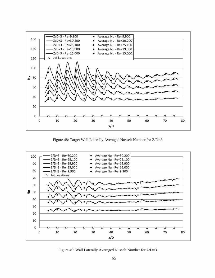
65
Figure 48: Target Wall Laterally Averaged Nusselt Number for Z/D=3
Figure 49: Wall Laterally Averaged Nusselt Number for Z/D=3
0
20
40
60
80
100
120
140
160
0 10 20 30 40 50 60 70 80
Nu
x/D
Z/D=3 - Re=9,900 Average Nu - Re=9,900 Z/D=3 - Re=30,200 Average Nu - Re=30,200 Z/D=3 - Re=25,100 Average Nu - Re=25,100 Z/D=3 - Re=19,900 Average Nu - Re=19,900 Z/D=3 - Re=15,000 Average Nu - Re=15,000 Jet Locations
0
10
20
30
40
50
60
70
80
90
100
0 10 20 30 40 50 60 70 80
Nu
x/D
Z/D=3 - Re=30,200 Average Nu - Re=30,200 Z/D=3 - Re=25,100 Average Nu - Re=25,100 Z/D=3 - Re=19,900 Average Nu - Re=19,900 Z/D=3 - Re=15,000 Average Nu - Re=15,000 Z/D=3 - Re=9,900 Average Nu - Re=9,900 Jet Locations

66
Figure 50: Target Wall Laterally Averaged Nusselt Number for Z/D=5
Figure 51: Wall Laterally Averaged Nusselt Number for Z/D=5
0
20
40
60
80
100
120
140
0 10 20 30 40 50 60 70 80
Nu
x/D
Z/D=5 - Re=10,000 Average Nu - Re=10,000
Z/D=5 - Re=30,000 Average Nu - Re=30,000
Z/D=5 - Re=24,800 Average Nu - Re=24,800
Z/D=5 - Re=19,900 Average Nu - Re=19,900
Z/D=5 - Re=15,000 Average Nu - Re=15,000
Jet Locations
0
10
20
30
40
50
60
70
80
0 10 20 30 40 50 60 70 80
Nu
x/D
Z/D=5 - Re=30,000 Average Nu - Re=30,000 Z/D=5 - Re=24,800 Average Nu - Re=24,800 Z/D=5 - Re=19,900 Average Nu - Re=19,900 Z/D=5 - Re=15,000 Average Nu - Re=15,000 Z/D=5 - Re=10,000 Average Nu - Re=10,000 Jet Locations

67
Figure 52: Target Wall Laterally Averaged Nusselt Number for Z/D=7
Figure 53: Wall Laterally Averaged Nusselt Number for Z/D=7
0
10
20
30
40
50
60
70
80
90
100
0 10 20 30 40 50 60 70 80
Nu
x/D
Z/D=7 - Re=10,000 Average Nu - Re=10,000 Z/D=7 - Re=29,900 Average Nu - Re=29,900 Z/D=7 - Re=25,100 Average Nu - Re=25,100 Z/D=7 - Re=19,900 Average Nu - Re=19,900 Z/D=7 - Re=15,000 Average Nu - Re=15,000 Jet Locations
0
10
20
30
40
50
60
70
80
0 10 20 30 40 50 60 70 80
Nu
x/D
Z/D=7 - Re=29,900 Average Nu - Re=29,900 Z/D=7 - Re=25,100 Average Nu - Re=25,100 Z/D=7 - Re=19,900 Average Nu - Re=19,900 Z/D=7 - Re=15,000 Average Nu - Re=15,000 Z/D=7 - Re=10,000 Average Nu - Re=10,000 Jet Locations

68
Figure 54: Target Wall Laterally Averaged Nusselt Number for Z/D=9
Figure 55: Wall Laterally Averaged Nusselt Number for Z/D=9
0
10
20
30
40
50
60
70
80
0 10 20 30 40 50 60 70 80
Nu
x/D
Z/D=9 - Re=10,000 Average Nu - Re=10,000
Z/D=9 - Re=30,000 Average Nu - Re=30,000
Z/D=9 - Re=25,100 Average Nu - Re=25,100
Z/D=9 - Re=20,100 Average Nu - Re=20,100
Z/D=9 - Re=15,000 Average Nu - Re=15,000
Jet Locations
0
10
20
30
40
50
60
0 10 20 30 40 50 60 70 80
Nu
x/D
Z/D=9 - Re=30,000 Average Nu - Re=30,000
Z/D=9 - Re=25,100 Average Nu - Re=25,100
Z/D=9 - Re=20,100 Average Nu - Re=20,100
Z/D=9 - Re=15,000 Average Nu - Re=15,000
Z/D=9 - Re=10,000 Average Nu - Re=10,000
Jet Locations

69
APPENDIX C: TABULATED NUSSELT NUMBER DATA

70
Table 7: Z/D=1 Target Wall Pitch Averaged Nusselt Number
Z/D=1 Target Wall Pitch Averaged Nusselt Number
Jet No Re=14,500
Re=12,500
Re=10,100 Re=7,400 Re=4,900
1 28.00 23.62 17.52 13.84 11.36
2 28.34 24.17 18.34 14.14 10.91
3 28.46 24.29 18.62 14.35 10.71
4 31.15 26.60 20.34 15.63 11.47
5 33.72 28.91 21.96 16.92 12.46
6 37.32 32.25 24.52 18.86 13.94
7 41.20 35.79 27.24 21.12 15.71
8 45.08 39.55 30.12 23.53 17.57
9 49.46 44.03 33.44 26.32 19.75
10 53.90 48.60 36.95 29.20 21.90
11 58.96 53.95 41.33 32.77 24.55
12 64.89 60.25 46.30 36.79 27.54
13 72.37 68.13 52.13 41.54 31.08
14 80.51 76.16 57.61 46.32 34.69
15 94.24 89.12 65.81 52.35 39.04
Area Avg 49.84 45.03 34.15 26.91 20.18
Table 8: Z/D=1 Side Wall Pitch Averaged Nusselt Number
Z/D=1 Side Wall Pitch Averaged Nusselt Number
Jet No Re=14,500
Re=12,500
Re=10,100 Re=7,400 Re=4,900
1 20.74 17.23 10.17 7.79 7.30
2 23.32 19.41 11.70 8.60 7.42
3 23.97 20.20 12.51 9.42 8.03
4 25.06 21.18 13.35 10.06 8.53
5 27.32 23.12 14.52 11.00 9.09
6 31.30 27.15 17.28 13.17 10.86
7 33.02 28.47 18.43 14.11 11.98
8 35.17 30.54 19.91 15.33 13.08
9 36.84 32.36 21.17 16.44 14.16
10 38.95 34.64 22.73 17.75 15.22
11 40.83 36.65 24.09 18.94 16.24
12 44.66 40.74 26.90 21.21 17.96
13 49.55 46.10 30.64 24.31 20.51
14 58.48 55.58 37.07 29.73 25.25
15 73.00 69.00 46.00 37.00 32.00
Area Avg 37.48 33.49 21.76 16.99 14.51

71
Table 9: Z/D=2 Target Wall Pitch Averaged Nusselt Number
Z/D=2 Target Wall Pitch Averaged Nusselt Number
Jet No Re=29,400
Re=24,900
Re=19,900
Re=15,000
Re=10,000
1 102.80 85.79 69.58 53.34 38.76
2 106.00 88.55 71.77 54.63 40.03
3 105.92 87.97 70.44 52.58 38.34
4 101.37 83.88 67.22 50.19 36.82
5 95.85 79.41 64.17 48.64 36.33
6 97.93 81.96 66.53 50.29 37.31
7 98.11 82.16 66.81 50.80 37.81
8 101.50 84.83 69.08 52.41 39.09
9 105.88 87.96 71.89 54.40 40.70
10 109.53 90.86 74.19 56.12 41.97
11 112.93 93.99 76.21 57.79 43.16
12 117.85 98.28 79.13 59.94 44.72
13 123.40 103.36 82.84 62.73 46.67
14 129.58 108.52 86.67 65.43 48.74
15 133.61 114.73 91.72 67.66 50.72
Area Avg 109.48 91.48 73.88 55.80 41.41
Table 10: Z/D=2 Side Wall Pitch Averaged Nusselt Number
Z/D=2 Side Wall Pitch Averaged Nusselt Number
Jet No Re=29,400
Re=24,900
Re=19,900
Re=15,000
Re=10,000
1 76.63 61.48 51.12 38.44 28.73
2 80.44 65.46 54.65 41.06 31.17
3 76.45 61.97 51.43 38.05 28.79
4 73.16 59.29 49.28 37.19 28.55
5 72.16 58.59 49.04 37.43 28.99
6 72.55 59.10 50.17 37.25 28.14
7 74.03 60.63 50.27 38.03 28.98
8 75.19 61.56 51.21 38.99 29.71
9 77.13 62.78 52.29 39.78 30.20
10 78.68 63.78 52.94 40.14 30.53
11 81.00 65.31 54.26 41.10 31.46
12 85.90 68.95 56.93 42.92 32.85
13 93.83 74.64 61.42 46.07 35.32
14 99.69 79.12 65.09 48.74 37.52
15 103.86 82.35 67.51 50.58 39.06
Area Avg 81.38 65.67 54.51 41.05 31.33

72
Table 11: Z/D=3 Target Wall Pitch Averaged Nusselt Number
Z/D=3 Target Wall Pitch Averaged Nusselt Number
Jet No Re=30,200
Re=25,100
Re=19,900
Re=15,000 Re=9,900
1 91.36 69.54 58.26 47.95 35.49
2 92.05 75.35 63.14 51.32 37.57
3 94.56 80.28 67.38 54.39 39.37
4 93.91 80.80 67.26 53.44 38.25
5 85.70 74.16 61.99 49.51 36.24
6 84.93 74.07 62.03 49.65 36.07
7 84.50 73.89 61.93 49.58 36.13
8 84.15 73.69 61.82 49.44 35.99
9 83.52 73.23 61.60 49.08 35.76
10 82.36 72.19 60.72 48.28 35.11
11 82.08 71.73 60.24 47.93 34.77
12 82.51 71.98 60.31 47.90 34.70
13 84.28 73.51 61.47 48.95 35.49
14 86.52 75.51 63.09 50.32 36.50
15 88.23 77.02 64.36 51.37 37.26
Area Avg 86.71 74.46 62.37 49.94 36.31
Table 12: Z/D=3 Side Wall Pitch Averaged Nusselt Number
Z/D=3 Side Wall Pitch Averaged Nusselt Number
Jet No Re=30,200
Re=25,100
Re=19,900
Re=15,000 Re=9,900
1 59.58 52.20 43.45 35.65 24.16
2 63.15 55.89 46.38 37.77 25.78
3 63.75 56.13 46.24 37.42 25.44
4 62.76 55.09 44.97 35.84 24.45
5 63.58 56.00 45.75 36.44 24.93
6 62.03 54.62 44.57 35.68 24.43
7 62.02 54.66 44.53 35.75 24.52
8 61.50 54.22 44.42 35.54 24.35
9 62.23 54.78 44.98 35.78 24.46
10 63.21 55.64 45.71 36.31 24.81
11 63.51 55.89 46.02 37.01 25.18
12 64.14 56.47 46.58 37.41 25.59
13 65.19 57.41 47.45 37.44 25.48
14 66.97 58.92 48.71 38.36 26.02
15 67.98 59.82 49.26 38.92 26.38
Area Avg 63.44 55.85 45.93 36.75 25.07

73
Table 13: Z/D=5 Target Wall Pitch Averaged Nusselt Number
Z/D=5 Target Wall Pitch Averaged Nusselt Number
Jet No Re=30,000
Re=24,800
Re=19,900
Re=15,000
Re=10,000
1 93.27 85.32 70.22 58.33 56.09
2 85.65 74.47 61.31 50.73 46.95
3 83.95 72.98 60.03 49.66 45.59
4 79.93 69.46 56.83 46.47 41.59
5 72.57 63.03 51.57 41.68 35.80
6 68.81 59.74 48.76 39.49 33.78
7 64.63 56.08 46.31 37.66 32.15
8 61.86 53.66 44.15 35.70 30.20
9 58.48 50.70 41.93 34.02 28.53
10 55.27 47.89 39.73 32.23 26.88
11 53.34 46.20 38.30 31.02 25.87
12 52.32 45.31 37.55 30.38 25.31
13 51.91 44.95 37.19 30.06 25.05
14 51.94 44.97 37.15 29.98 24.92
15 54.30 47.05 38.80 31.33 25.93
Area Avg 65.88 57.45 47.32 38.58 33.64
Table 14: Z/D=5 Side Wall Pitch Averaged Nusselt Number
Z/D=5 Side Wall Pitch Averaged Nusselt Number
Jet No Re=30,000
Re=24,800
Re=19,900
Re=15,000
Re=10,000
1 45.80 39.71 32.49 26.46 19.71
2 48.42 42.05 34.54 28.23 21.27
3 49.38 43.23 35.85 29.33 22.05
4 49.10 42.93 35.73 29.27 22.23
5 49.23 42.55 35.85 29.57 22.48
6 50.73 42.55 35.15 28.33 21.15
7 48.70 41.91 34.67 28.12 21.29
8 47.93 41.48 34.34 27.63 20.87
9 48.37 42.30 34.91 28.17 21.45
10 48.34 42.40 35.06 28.36 21.56
11 47.84 41.93 34.62 28.02 21.25
12 48.77 42.64 35.20 28.53 21.67
13 49.64 43.24 35.67 28.90 21.92
14 50.68 44.01 36.26 29.35 22.19
15 51.89 45.02 37.08 29.98 22.55
Area Avg 48.99 42.53 35.16 28.55 21.58

74
Table 15: Z/D=7 Target Wall Pitch Averaged Nusselt Number
Z/D=7 Target Wall Pitch Averaged Nusselt Number
Jet No Re=29,900
Re=25,100
Re=19,900
Re=15,000
Re=10,000
1 79.71 64.83 53.38 41.68 30.74
2 78.64 64.50 53.17 41.53 30.62
3 78.41 64.26 53.20 41.72 30.93
4 76.08 62.47 51.33 40.09 29.37
5 70.22 57.35 47.01 36.73 26.72
6 64.61 52.71 43.14 33.92 24.67
7 61.50 50.01 40.91 32.22 23.42
8 58.28 47.29 38.67 30.53 22.10
9 54.06 43.94 35.97 28.50 20.55
10 49.79 40.66 33.27 26.33 18.95
11 47.26 38.70 31.63 24.98 18.00
12 45.01 36.86 30.12 23.74 17.09
13 43.35 35.31 28.82 22.66 16.29
14 42.42 34.35 27.90 21.92 15.68
15 42.52 34.05 27.55 21.63 15.39
Area Avg 59.46 48.49 39.74 31.21 22.70
Table 16: Z/D=7 Side Wall Pitch Averaged Nusselt Number
Z/D=7 Side Wall Pitch Averaged Nusselt Number
Jet No Re=29,900
Re=25,100
Re=19,900
Re=15,000
Re=10,000
1 42.91 36.18 30.23 24.12 17.89
2 45.28 38.40 32.15 25.75 18.98
3 44.08 37.40 31.48 25.28 18.75
4 45.12 38.27 32.26 25.99 19.25
5 46.10 39.13 33.20 26.80 19.87
6 46.57 39.51 33.40 26.94 20.04
7 46.53 39.39 33.27 26.78 19.85
8 45.87 38.84 32.75 26.31 19.45
9 45.98 38.84 32.70 26.25 19.34
10 46.08 38.88 32.68 26.18 19.24
11 46.49 39.25 32.95 26.36 19.35
12 47.00 39.60 33.25 26.54 19.42
13 47.25 39.68 33.31 26.53 19.34
14 46.44 38.87 32.54 25.91 18.81
15 46.43 38.72 32.39 25.77 18.66
Area Avg 45.88 38.73 32.57 26.10 19.21

75
Table 17: Z/D=9 Target Wall Pitch Averaged Nusselt Number
Z/D=9 Target Wall Pitch Averaged Nusselt Number
Jet No Re=30,000
Re=25,100
Re=20,100
Re=15,000
Re=10,000
1 57.74 49.53 41.81 33.48 24.68
2 56.93 48.85 41.36 33.09 24.57
3 56.19 48.20 40.71 32.54 24.22
4 54.64 46.76 39.48 31.42 23.40
5 51.63 44.12 37.27 29.61 22.24
6 49.21 42.12 35.54 28.30 21.31
7 47.03 40.24 33.87 26.95 20.31
8 44.47 38.03 31.92 25.28 19.10
9 42.16 36.05 30.26 23.89 18.04
10 39.63 33.84 28.20 22.11 16.66
11 37.54 31.97 26.54 20.71 15.51
12 35.37 30.04 24.86 19.31 14.34
13 34.44 29.23 24.12 18.68 13.85
14 33.45 28.37 23.31 17.96 13.27
15 32.75 27.68 22.62 17.33 12.74
Area Avg 44.88 38.34 32.12 25.38 18.95
Table 18: Z/D=9 Side Wall Pitch Averaged Nusselt Number
Z/D=9 Side Wall Pitch Averaged Nusselt Number
Jet No Re=30,000
Re=25,100
Re=20,100
Re=15,000
Re=10,000
1 36.08 31.50 26.12 21.06 16.07
2 37.99 33.11 27.51 22.26 16.85
3 37.20 32.40 26.88 21.78 16.35
4 36.71 31.91 26.53 21.50 16.10
5 36.79 31.93 26.50 21.47 16.01
6 38.02 33.00 27.50 22.34 16.73
7 38.67 33.56 27.98 22.74 16.98
8 38.11 33.03 27.51 22.33 16.65
9 38.47 33.31 27.72 22.47 16.73
10 38.21 33.10 27.53 22.26 16.58
11 38.58 33.39 27.74 22.37 16.64
12 38.33 33.17 27.51 22.17 16.47
13 36.99 31.97 26.46 21.26 15.71
14 37.30 32.23 26.68 21.40 15.78
15 37.88 32.71 27.06 21.69 15.95
Area Avg 37.69 32.69 27.15 21.94 16.37

76
APPENDIX D: ACTUAL REYNOLDS NUMBERS
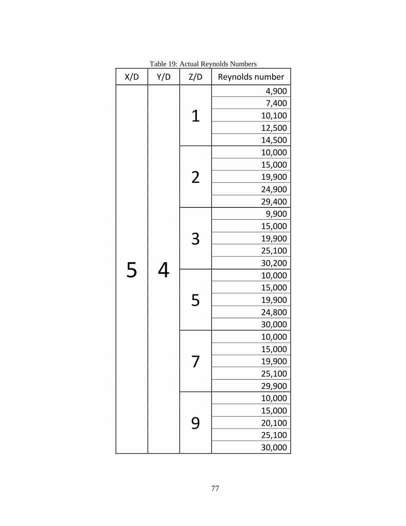
77
Table 19: Actual Reynolds Numbers
X/D Y/D Z/D Reynolds number
5 4
1
4,900
7,400
10,100
12,500
14,500
2
10,000
15,000
19,900
24,900
29,400
3
9,900
15,000
19,900
25,100
30,200
5
10,000
15,000
19,900
24,800
30,000
7
10,000
15,000
19,900
25,100
29,900
9
10,000
15,000
20,100
25,100
30,000

78
APPENDIX E: LATERAL CONDUCTION CALCULATIONS

79

80

81
REFERENCES
[1] U. E. I. Administration, "Annual energy Review," DOE/EIA-0384(2011), Washington DC,
2012.
[2] J. P. Downs and K. K. Landis, "Turbine Cooling Systems Design - Past, Present and
Future," in Proceedings of ASME Turbo Expo, GT2009-59991, 2009.
[3] R. S. Bunker, "Gas Tubine Heat Transfer: Ten Remaining Hot Gas Path Challenges,"
Journal of Turbomachinery, vol. 129, no. April, pp. 193-201, 2007.
[4] J. C. Han and S. E. S. Dutta, Gas Turbine Heat Transfer and Cooling Technology, New
York: Taylor & Francis, Inc., 2000.
[5] L. A. El-Gabri and D. A. Kaminski, "Numerical investigation of jet impingement with
crossflow - Comparison of Yang-Shih and standard k-e turbulence models,"
Numerical Heat Transfer, vol. 47, pp. 441-469, 2005.
[6] M. Zuckerman and N. Lior, "Impingement Heat Transfer: Correlations and Numerical
Modeling," Journal of Heat Transfer, vol. 124, p. 544, 2005.
[7] K. S. Mushatat, "Analysis of the turbulent flow and heat trasnfer of the impingement
cooling in a channel with cross flow," Journal of King Abdulaziz University, vol. 18,
no. 2, pp. 101-122, 2007.
[8] M. E. Taslim, K. Bakhatari and H. Liu, "Experimental and numerical investigation of
impingement on a rib-roughened leading-edge wall," Journal of Turbomachinery,
vol. 125, pp. 682-691, 2003.
[9] S. Acharya, A. Eshtiaghi and R. Schilp, "Flow distribution and heat transfer coefficients

82
inside gas holes discharging into an orthogonal cross flow," International Journal of
Heat and mass transfer, vol. 55, pp. 7036-7045, 2012.
[10] P. Gulati, V. Katti and S. Prabhu, "Influence of the shape of the nozzle on local heat transfer
distribution between smooth flat surface and impining air jet," International Journal
of Thermal Sciences, vol. 48, pp. 602-617, 2009.
[11] R. Herrero Martin and J. M. Buchlin, "Jet impingement heat transfer from lobed nozzles,"
International Journal of Thermal Sciences, vol. 50, pp. 1199-1206, 2011.
[12] J. Lee and S.-J. Lee, "The effect of nozzle configuration on stagnation region heat transfer
enhancement of axisymmetric jet impingement," International Journal of Heat and
Mass Transfer, vol. 43, pp. 3497-3509, 2000.
[13] H. Martin, "Heat and Mass Tranfer between Impinging Gas Jets and Solid Surfaces,"
Advances in Heat Transfer, 1977.
[14] R. Viskanta, "Heat Transfer to Impinging Isothermal Gas and Flame Jets," Experimental
Thermal and Fluid Science, vol. 6, pp. 111-134, 1993.
[15] B. Weigand, "Multiple Jet Impingement - A Review," Heat Transfer Research, vol. 42, no.
2, pp. 101-142, 2011.
[16] C. Carcasci, "An experimental investigation on air impinging jets using visualisation
methods," International Journal of Thermal Schience, vol. 38, pp. 808-818, 1999.
[17] L. Florschuetz, R. A. Berry and D. E. Metzger, "Periodic Streamwise Variations of Heat
Transfer Coefficients for Inline and Staggered Arrays of Circular Jets with Cross
Flow of Spent Air," Journal of Heat Transfer, vol. 102, pp. 132-137, 1980.

83
[18] L. W. Florschuetz, C. R. Truman and D. E. Metzger, "Streamwise Flow and Heat Transfer
Distributions for Jet Array Impingement with Cross flow," Journal of Heat Transfer,
vol. 103, p. 337, 1981.
[19] L. W. Florschuetz and Y. Isoda, "Flow Distributions and Discharge Coefficient for Jet
Array Impingement with Initial Cross Flow," Journal of Engineering for Power, vol.
105, p. 296, 1983.
[20] Y.-H. Liu, S.-J. Song and Y.-H. Lo, "Jet impingement heat transfer on target surfaces with
longitudinal and transverse grooves," International Journal of Heat and Mass
Transfer, vol. 58, pp. 292-299, 2013.
[21] D. E. Metzger and R. J. Korstad, "Effects of crossflow on impingement heat transfer,"
Journal of Engineering for Power, pp. 35-41, 1972.
[22] J.-Y. San and W.-Z. Shiao, "Effects of jet plate size and plate spacing on the stagnation
Nusselt number for a confined circular air jet impinging on a flat surface,"
International Journal of Heat and Mass Transfer, vol. 49, pp. 3477-3486, 2006.
[23] J.-Y. San and M.-D. Lai, "Optimum jet-to-jet spacing of heat transfer for ataggered arrays of
impinging air jets," International Journal of Heat and Mass Transfer, vol. 44, no.
21, pp. 3997-4007, 2001.
[24] K. W. Van Treuren, Z. Wang, P. Ireland, T. V. Jones and S. Kohler, "Comparison and
prediction of local and average heat transfer coefficients under an array of inline and
staggered impinging jets," in International Gas Turbine and Aeroengine Congress,
Birmingham, UK, 1996.

84
[25] A. C. Chambers, D. R. H. Gillespie, P. T. Ireland and G. M. Dailey, "The effect of initial
cross flow on the cooling performance of a narrow impingement channel," Journal
of Heat Transfer, vol. 127, pp. 358-365, 2005.
[26] J. Park, M. Goodro, P. Ligrani, M. Fox and H.-K. Moon, "Separate effects of Mach number
and Reynolds number on jet array impingement heat trasnfer," Journal of
Turbomachinery, vol. 129, pp. 269-280, 2007.
[27] M. Goodro, J. Park, P. Ligrani, M. Fox and H.-K. Moon, "Effects of hole spacing on
spatially-resolved jet array impingement heat transfer," International Journal of
Heat and Mass Transfer, vol. 51, pp. 6243-6253, 2008.
[28] H. H. Cho and D. H. Rhee, "Local heat/mass transfer measurement on the effusion plate in
impingement/effusion cooling systems," Journal of Turbomachinery, vol. 123, pp.
601-608, 2001.
[29] A. J. Onstand, C. J. Elkins, R. J. Moffat and J. K. Eaton, "Full-field flow measurements and
heat transfer of a compact jet impingement array with local extraction of spent
fluid," Journal of Heat Transfer, vol. 131, pp. 1-8, 2009.
[30] R. S. Bunker and D. E. Metzger, "Local heat transfer in internally cooled turbine airfoil
leading edge regions: Part I - Impingement cooling without film coolant extraction,"
Journal of Turbomachinery, vol. 112, pp. 451-458, 1990.
[31] D. E. Metzger and R. S. Bunker, "Local heat transfer in internally cooled turbine airfoil
leading edge regions: Part II - Impingement cooling with film coolant extraction,"
Journal of Turbomachinery, vol. 112, pp. 459-466, 1990.

85
[32] D. R. H. Gillespie, Z. Wang, P. T. Ireland and S. T. Kohler, "Full surface local heat transfer
coefficient measurements in a model of an integrally cast impingmeent cooling
geometry," Journal of Turbomachinery, vol. 120, pp. 92-99, 1998.
[33] H. Deng, Z. Gu, J. Zhu and Z. Tao, "Experiments on impingemnet heat transfer with film
extraction flow on the leading edge of rotating blades," International Journal of
Heat and Mass Transfer, vol. 55, pp. 5425-5435, 2012.
[34] M. Fenot, E. Dorignac and J.-J. Vullierme, "An experimental study on hot round jets
impinging a concage surface," International Journal of Heat and Mass Transfer, vol.
29, pp. 945-956, 2008.
[35] W. M. Yan and S. Mei, "Measurement of detailed heat transfer along rib-roughened surface
under arrays of impinging elliptic jets," International Journal of Heat and Mass
Transfer, vol. 49, pp. 159-170, 2006.
[36] W. M. L. H. S. C. Y. W. Yan, "Experimental study of impinging heat trasnfer along rib-
roughened walls by using transient liquid crystal technique," International journal of
Heat and Mass Transfer, vol. 48, pp. 2420-2428, 2005.
[37] K. Kanokjaruvijit and R. F. Martinez-Botas, "Jet impingement on a dimpled surface with
different crossflow schemes," International Journal of Heat and mass Transfer, vol.
48, pp. 161-170, 2005.
[38] A. P. Rallabandi, D.-H. Rhee, Z. Gao and J. Han, "Heat transfer enhancement in rectangular
channels with axial ribs or porous foam under through flow and impinging jet
conditions," International Journal of Heat and Mass Transfer, vol. 53, pp. 4663-
4671, 2010.

86
[39] S. V. Ekkad and D. Kontrovitz, "Jet impingement heat trasnfer on dimpled target surfaces,"
International journal of heat and Fluid Flow, vol. 23, pp. 22-28, 2002.
[40] K. V. Akella and J.-C. Han, "Impingement cooling in rotating Two-Pass Rectangular
Channels with Ribbed Walls," Journal of Thermophysics and Heat Transfer, vol. 13,
no. 3, pp. 364-371, 1999.
[41] Q. Liu, A. Sleiti and J. Kapat, "Application of pressure and temperature sensitive paints for
study of heat trasnfer to a circular impining air jet," International Journal of
Thermal Sciences, vol. 47, pp. 749-757, 2008.
[42] Q. Liu, Study of Heat Transfer Characteristics of Impinging Air Jet Using Pressure and
Temperature Sensitive Liminscent Paint, University of Central Florida Dissertation,
2006.
[43] F. Incropera, Fundamentals of Heat and Mass Tranfer, Hoboken: Wiley, 2006.
[44] M. Ricklick and J. Kapat, "Sidewall effects on heat transfer coefficient in a narrow
impingement channel," Journal of Thermophysics and Heat Transfer, vol. 24, no. 1,
pp. 123-132, 2010.
[45] B. D. Figliola R.S., Theory and Design for Mechanical Measurements, Hoboken: Wiley,
2006.