healthy people, healthy economies · this section provides information on a subset of solutions ......
TRANSCRIPT

SM
HEALTHY PEOPLE, HEALTHY ECONOMIES
This report was written and prepared by:

Contact Information CLIENT SERVICES Representatives are available: 7AM to 7PM EST (12PM-12AM GMT), Mon-Fri.Email [email protected] or contact us at a location below:
U.S. & Canada +1.866.275.3266 or +1.610.235.5299EMEA (London) +44.20.7772.1646 (Prague) +420.224.222.929Asia/Pacifi c +61.2.9270.8111
WORLDWIDE OFFICES
West Chester 121 N. Walnut St., Suite 500, West Chester PA 19380 +1.610.235.5000United KingdomOne Canada Square, Canary Wharf, London E14 5FA +44.20.7772.5454AustraliaLevel 10, 1 O’Connell Street, Sydney, NSW, 2000 Australia +61.2.9270.8111PragueWashingtonova 17, 110 00 Prague 1, Czech Republic +420.224.222.929
MOODY’S ANALYTICS
Products & ServicesThis section provides information on a subset of solutions from Moody’s Analytics. Visit moodysanalytics.com for a full listing of all solutions offered by the company.
ECONOMIC FORECAST DATABASESGlobal Macro Forecast Database*Global Metropolitan Areas Forecast DatabaseU.S. Macro Forecast Database*U.S. State Forecast Database*U.S. Metropolitan Areas Forecast Database*U.S. State & Metro Detailed Employment Forecast DatabaseU.S. County Forecast DatabaseU.S. County Detailed Employment Forecast DatabaseCase-Shiller® Home Price Indexes* (U.S.)CreditForecast.com* (U.S.)Forecasts of RCA CPPI™ Housing Stock Forecast Database (U.S.)RealtyTrac Foreclosures (U.S.)*With Alternative Scenarios
ECONOMIC HISTORICAL DATABASESGlobal National & Subnational DatabaseU.S. National & Regional DatabaseAmerican Bankers Association Delinquency Database (U.S.)Case-Shiller® Home Price Indexes (U.S.)CoreLogic Home Price Indexes (U.S)CreditForecast.com (U.S.)LPS Home Price Indexes (U.S.)National Association of Realtors:
Pending Home Sales (U.S.)Monthly Supply of Homes (U.S.)
Data packages can be customized to clients’ geographic areas of interest.
ECONOMIC MODELS & WORKSTATIONSU.S. Macro & State ModelU.S. Regional WorkstationWorld WorkstationMoody’s CreditCycle™
ECONOMIC RESEARCHEconomy.com (Global)Précis® Macro (U.S.)Précis® Metro (U.S.)Précis® State (U.S.)Regional Financial Review®
ECONOMIC ADVISORY SERVICESClient PresentationsConsumer Credit AnalyticsCredit Risk ManagementCustom Scenarios Economic Development AnalysisMarket AnalysisProduct Line ForecastingStress-Testing
EventsECONOMIC OUTLOOK CONFERENCEOur two-day fl agship event, providing comprehensive insight on all the components that drive macro and regional economies.
Philadelphia PA May 2017
REGIONAL ECONOMIC OUTLOOK CONFERENCEA full day event, providing comprehensive insight on the components that drive regional economies.
West Chester PA October 2016
Visit www.economy.com/events for listings, details and registration.
ECONOMIC BRIEFINGSHalf- and full-day events designed to provide comprehensive insight on the macro and regional economies.
REGIONAL ECONOMIC BRIEFINGSHalf-day events designed to provide detailed insight into an individual area’s current and expected economic conditions.
SPEAKING ENGAGEMENTSEconomists at Moody’s Analytics are available for your engagement. Our team of economists has extensive experience in making presentations on a variety of topics, including: macro outlook, consumer outlook, credit cycles, banking, housing/real estate, stress testing, sovereign credit, and regional economies. Contact us for more information.

BCBS �� Healthy People, Healthy Economies
MOODY’S ANALYTICS / Copyright© 2016
Table of Contents
Executive Summary .......................................................................................................... 1
Healthy People, Healthy Economies ............................................................................. 4
Healthy People, Healthy Incomes ..................................................................................9
Healthy People, Healthy Workforce .............................................................................13
Appendix .......................................................................................................................... 17
BCBS �� Executive Summary
MOODY’S ANALYTICS / Copyright© 2016 1
Executive Summary
Researchers and economists have long held the belief that there is a strong relationship between the health of a population and the health of an economy. This study aims to confirm the statistical relationship between those two concepts, as well as gain insight into any causal relationships that might exist by
breaking the data down across three different dimensions:
» Healthy people, healthy economies » Healthy people, healthy incomes » Healthy people, healthy workforce
Such an analysis is made possible by a new groundbreaking health metric from the Blue Cross Blue Shield Association. The BCBS Health Index provides a detailed and data-driven way to objectively measure health across the U.S. The health index cap-tures the relative health of BCBS members in nearly every county in the U.S. using rig-orous statistical analysis and health insur-ance data from millions of members. This new measure has tremendous potential to
help academics, policymakers and industry better understand how health affects a variety of outcomes at the local level. In particular, it can help develop a better un-derstanding of how a healthy population is related to a strong local economy.
Healthy people, healthy economiesA wide literature suggests that the
healthiness of a population should be related to the performance of the local economy. There are a variety of ways that health can contribute to the economy, and in turn many ways that the economy can contribute to health outcomes.
The most direct connection between health and the economy is that healthier populations mean healthier workers, and healthier workers, in turn, are likely to be more productive and employed. Poor health weighs on physical and mental strength, which is essential to job performance in many occupations.
Less-healthy workers are also more likely to have more frequent absences from work, which will further hurt productivity and pay. In addition, when poor health causes longer absences from the workforce, this can lead to the deterioration of job skills and trouble getting re-employed.
Finally, mental and physical health can affect the accumulation of education and other skills. Just as poor health can cause significant absences from work, it can do the same for school. Mental health contributes to success in school, which can increase edu-cational and skill attainment.
While better health is likely to con-tribute to positive outcomes in the local economy, the effects likely go both ways. A strong economy means better jobs, which are more likely to provide health insur-ance and the means and education to live a healthier lifestyle.
Healthier populations contribute to a stronger local economy, and a stronger local economy contributes to a healthier popula-tion. An important step in understanding this relationship is measuring the correlation between the two.
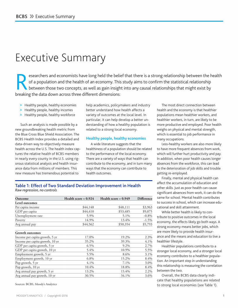
Overall, the BCBS data clearly indi-cate that healthy populations are related to strong local economies (see Table 1).
Table 1: Effect of Two Standard Deviation Improvement in HealthRaw regression, no controls
Outcome Health score = 0.924 Health score = 0.949 DifferenceLevel outcomesPer capita income $44,148 $48,111 $3,963GDP per capita $44,410 $53,485 $9,075Unemployment rate 5.9% 5.1% -0.8%Poverty 14.9% 13.4% -1.5%Avg annual pay $44,562 $50,354 $5,793
Growth outcomesIncome per capita growth, 5 yr 17.0% 19.2% 2.3%Income per capita growth, 10 yr 35.2% 39.3% 4.1%GDP per capita growth, 5 yr 6.5% 9.2% 2.7%GDP per capita growth, 10 yr 5.4% 10.9% 5.5%Employment growth, 5 yr 5.5% 8.6% 3.1%Employment growth, 10 yr 6.8% 15.2% 8.4%Pop growth, 5 yr 4.1% 7.1% 3.0%Pop growth, 10 yr 10.4% 18.8% 8.4%Avg annual pay growth, 5 yr 13.2% 15.4% 2.2%Avg annual pay growth, 10 yr 30.5% 34.1% 3.6%
Sources: BCBS, Moody’s Analytics

MOODY’S ANALYTICS / Copyright© 2016 2
Where populations are healthier, we ob-serve lower unemployment, higher income and higher pay. Moving from a county of average health to the 99th percentile is associated with an increase in average an-nual pay of $5,793 and a 0.8-percentage point decline in the unemployment rate (see Chart 1).
Even after controlling for demograph-ics and statewide factors, the correlation is robust for most outcomes. The association between health and the pace of economic growth is even stronger. Healthier areas tend to have faster job growth, population growth and income growth even compared with areas with similar demographics within the same state.
The effect of specific health conditions on economic growth were also examined, with mixed results. However, these mixed results for conditions validate the importance of BCBS efforts to create a single health index that summarizes across all conditions into a single measure.
These results do not prove a causal rela-tionship between healthy populations and strong local economies. However, the ro-bustness of many measures to demographic controls and state fixed effects does give more reason to suspect a causal relationship may exist.
Healthy people, healthy incomesHaving established a correlation be-
tween healthy people and healthy econo-mies, the next step in our analysis is to try and establish some type of causal relation-
ship between the two. In addition to geographic detail, the 26-mil-lion member BCBS dataset also provides informa-tion on members’ industry of em-ployment, which is a valuable level of granularity in assessing the rela-tionship between health and wages.
The availabil-ity of industry-level granularity provides a greater number of datapoints on which to test the causality between health and in-comes, and also allows for models that con-trol for very local geographic differences and differences among industries.
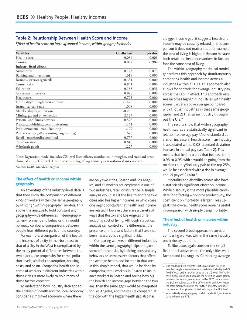
The within-geography models show a consistently statistically significant relation-
ship between income and health despite the strong test of including local geographical fixed effects (see Table 2). Increasing health scores from 0.93 to 0.95, which would be going from the median county/industry pair to the top 25%, is associated with an increase in average annual pay of $1,400. These within-geography results also hold if only a subset of conditions are used that are predominately driven by genetic factors as opposed to behavioral factors. This is sugges-tive, though not dispositive, of a causal effect of health on incomes.
Within-industry models are also sug-gestive, but the results here are more mixed with statistical significance only in some industries and only using some health score measures. The difficulty in finding consistent statistically signifi-cant results between industries suggests several possible limitations of the data and methodology that could be resolved by looking at these issues at a more granular level.
Table 2: Relationship Between Health Score and IncomeEffect of health score on log avg annual income, within-geography model
Variables Coefficient p-valueHealth score 0.084 0.001Constant 0.002 0.982Industry fixed effectsAutomotive 0.123 0.073Banking and investment 1.619 0.000Business services (general) -0.331 0.000Construction 0.801 0.000Education 0.183 0.051Government services 0.878 0.000Healthcare 0.708 0.000Hospitality/dining/entertainment -1.428 0.000Insurance/real estate 1.008 0.000Membership organizations -0.206 0.088Mining/gas & oil extraction 2.127 0.000Personal and family services -0.576 0.000Printing/publishing/communications 1.161 0.000Product/material manufacturing 1.179 0.000Professional (legal accounting engineering) 1.673 0.000Retail - merchandise & food -0.757 0.000Transportation 0.615 0.000Wholesale Goods 1.227 0.000
Note: Regression model includes CZ level fixed effects, member count weights, and standard areas clustered at the CZ level. Health score and log of avg annual pay transformed into z-scores. Sources: BCBS, Moody’s Analytics
11
0
2
4
6
8
10
12
14
16
0.88 0.90 0.92 0.94 0.96
Chart 1: Unemployment Falls, Health Score RisesX-axis: health score; Y-axis: unemployment rate
Sources: BLS, BCBS, Moody’s Analytics
Scaled by number
of members in the county
BCBS �� Executive Summary

MOODY’S ANALYTICS / Copyright© 2016 3
First, the previous results notwithstand-ing, it remains unclear the extent to which health causes income versus income causing health. Second, state-level differences in coverage and other unmeasured factors may be clouding the results. Finally, the industry-level differences rely on fewer observa-tions than the within-geography analysis, which makes identifying significant effects more challenging.
Overall, there is some suggestive evi-dence of a causal relationship from health to income, though there remains a significant amount of uncertainty given the challenge of teasing out causality in such a complex and nuanced relationship. More persuasive evidence of a causal relationship will require increasing levels of granularity, including detailed firm-level data and tracking data over time.
Healthy people, healthy workforceThe BCBS Health Index also gives us the
opportunity to further examine causality by measuring the impact on employment and participation in the workforce from health outcomes across different age co-horts. Given the rapid aging of the Ameri-can workforce, the supply of labor needed to achieve historical averages of economic growth will require more U.S. workers to keep working later in life than ever before. Geographic areas that are able to best harness this cohort of aging workers stand the best chance of sustaining a respect-able pace of economic growth as the over-all workforce ages in the years ahead. It stands to reason that older workers can do this only if they remain healthy enough to continue working.
Comparing health scores and the percentage of individuals em-ployed across age cohorts shows that the two concepts have an important positive correla-tion, especially among older work-ing-age Americans, those between the ages of 45 and 60 (see Chart 2).
We estimate that an increase of two stan-dard deviations in a county’s health index corresponds to an increase in employment for the 55 to 64 cohort by 0.7%. Using a standard employment elasticity, this 0.7% increase will roughly translate into an extra 1.5% increase in economic growth. However, this relationship can change based on where we are in the business cycle, and given the current pace of sluggish productivity growth, the output gains from employment today are likely less than standard estimates.
The increased importance of health on employment among older populations ver-sus younger populations can be used as evi-dence that the flow of causality runs from health to employment rather than employ-ment causing better health. If the causality flowed only one way, from employment to good health, our model would be equally sensitive to the exclusion of any age group if it is assumed that the tangible, social and mental benefits from employment remain relatively static or even improve as you age. However, the same cannot be said about
health, which has yet to notch a win against Father Time. Healthy workers lead to in-creased employment, especially among old-er workers, which in turn leads to increased economic growth.
Ultimately, what this study establishes is that health outcomes and economic out-comes are directly related. Causality flow-ing in one direction cannot be definitively established, but we instead see causality most likely runs both ways. Healthy people have the ability to work longer and derive better economic outcomes for themselves over time, while simultaneously, access to employer-paid insurance and the where-withal to live a healthier lifestyle can be at least somewhat attributed to having gainful employment. Which of these causal flows is most dominant likely depends on individual circumstances at the geographical, firm and personal level. Additional work can be done on firm- and individual-level data that can shed more light on what influences these flows, and how health can in turn influence economic growth.
22
-0.2 -0.1 0.0 0.1 0.2 0.3
60-64
55-64
55-59
45-54
35-44
30-34
25-34
25-29
20-29
20-24
Significant at 1%
Significant at 5%
Not significant
Chart 2: Health and Employment Correlations
Sources: BCBS, ACS, Moody’s Analytics
Pearson correlation health index and % employed by age
BCBS �� Executive Summary

BCBS �� Healthy People, Healthy Economies
MOODY’S ANALYTICS / Copyright© 2016 4
Healthy People, Healthy Economies
Researchers and economists have long held a strong relationship between the health of a population and the health of an economy. This study aims to confirm the statistical relationship between those two concepts, as well as gain insight into any causal relationships that might exist. However, Part 1 will focus
solely on establishing a statistical foundation for that relationship, using a new groundbreaking health metric from Blue Cross Blue Shield Association. The BCBS Health Index provides a detailed and data-driven way to measure health across the U.S. The health index captures the relative health of nearly every county in the U.S. using rigorous statistical analysis and health insurance data from millions of members. This new measure has tremendous potential to help academics, policymakers and the industry better understand how health affects a variety of outcomes at the local level. In particular, it can help develop a better understanding of how a healthy population is related to a strong local economy.
Understanding the health indexThe BCBS Health Index data analyzed by
Moody’s Analytics is derived from admin-istrative health records from more than 25 million BCBS members.1 The administrative records allow detailed and thorough mea-surement of current and past medical condi-tions for each member. These conditions are combined with disability information from the Institute of Health Metrics and Evalu-ation and cause of death information from the Centers for Disease Control to create disability and mortality scores.
Mortality and disability scores are com-bined to create an overall health index.
Numerically, the health index is equal to the ratio of expected remaining healthy years of life (after accounting for any mor-tality risk or disability) divided by the num-ber of years that an individual would have under optimal health. The more healthy years of life that are lost because of medical conditions, the lower the health index.
For example, consider an individual whose current medical conditions and age imply 27 years of healthy life remain-ing but who would have 30 years under
1 The data are restricted to individuals who were members for the full year.
optimal health. The health index would be 0.9 (27/30), because 10% of the remaining years of healthy life are expected to be lost to mortality and disability. If instead that in-dividual had 28.5 expected years of healthy life remaining, the health index would be 0.95 (28.5/30), suggesting a 5% loss due to health conditions.
Data coverageThe data analyzed by Moody’s Analytics
include average health indexes, mortality scores, and disability scores at the county level. The 25 million full-year members repre-sent 8.2% of the population in the 3,140 U.S. counties for which data are available.2 Health indexes are available in all 50 states and the District of Columbia, with a wide range of coverage ratios. The wide range of coverage is controlled in this analysis by weighting geographies based on the number of persons covered. This helps eliminate potential distor-tions in the findings from counties with rela-tively low member counts.
The level of coverage in a county is re-lated to the poverty rate in the county. An
2 Not all BCBS plans are represented in this data, leaving smaller than expected counts for some states. More obser-vations across geographies will be added to future iterations of the score as additional plans opt in.
increase in county poverty of 1 percentage point decreases BCBS health coverage by 0.3 percentage point. However, when the percentage of the population without in-surance is controlled for, poverty becomes statistically insignificant. This suggests that an overall lack of health insurance is why higher-poverty counties have less coverage in the BCBS data. Personal income, average pay, and median household income are not statistically related to coverage.
Wide disparities in outcomesThe average county health index is
0.925, and the median is 0.926. County health indexes range from 0.84 to 0.99, however this wide range reflects a hand-ful of outliers that arise from small sample sizes. A better measure of the range of out-comes is the difference between the 10th and 90th percentiles, which are 0.907 and 0.941, respectively (see Table 1). This means the residents of the county with the 90th percentile of health index can expect 3.4 percentage points more healthy years of life than those in the 10th percentile.
The difference in healthcare costs in healthy and less healthy counties provides a measure of the economic importance of this disparity. In a county in the 90th percentile

BCBS �� Healthy People, Healthy Economies
MOODY’S ANALYTICS / Copyright© 2016 5
of health index, average healthcare costs as provided by BCBS are 6% lower than for a county in the 10th percentile.
Among the 100 largest counties in the U.S., the average health index is 0.924, slightly lower than the overall average. Among these counties, the lowest health index is Suffolk County NY with a health in-dex of 0.89 and the healthiest is Santa Clara County CA with a health index of 0.95.
Geographically, health indexes tend to cluster strongly and exhibit a clear spatial pat-tern. Health indexes are lower in the South-east and up through the Atlantic and even the Northeast. The Midwest, Central and Moun-tain states are healthier (see Chart 1).
Healthy population and a strong econ-omy
A wide literature suggests that the healthiness of a population should be related to the performance of the local economy. There are a variety of ways that health can contribute to the economy, and in turn many ways that the economy can contribute to health outcomes.
The most direct connection between health and the economy is that healthier populations mean healthier workers, and healthier workers, in turn, are likely to be more productive and employed. Poor health weighs on physical and mental strength that are essential to job performance in many occupations.
Less healthy workers are also more likely to have more frequent absences from work, which will further hurt productivity and pay. In addition, when poor health causes longer absences from the workforce, this can lead to the deterioration of job skills and trouble getting re-employed. For example, research has shown that workers who leave the labor force in order to apply for disability insurance later struggle to find work even if they do not end up qualifying for disability.3
Finally, mental and physical health can af-fect the accumulation of education and other
3 D. Autor, N. Maestas, K.J. Mullen, and A. Strand, “Does Delay Cause Decay? The Effect of Administrative Decision Time on the Labor Force Participation and Earnings of Disability Applicants,” National Bureau of Economic Research working paper No. w20840, 2015.
skills. Just as poor health can cause significant absences from work, it can do the same for school. Research has shown that children who sustain major injuries have statis-tically significantly worse educational outcomes compared to unaffected sib-lings.4 In addition to physical health, mental health contributes to success in school, which can increase educational and skill attainment. For example, children diagnosed with ADHD or conduct disorder have a literacy score that is half a standard deviation lower than unaf-fected siblings.5
While better health is likely to contribute to positive outcomes in the local economy, the effects likely go both ways. A strong economy means better jobs, which are more likely to provide health insurance. Higher pay also makes investment in education easier, which in turn improves health and income. For example, research has shown that com-pulsory schooling laws increased health and life expectancy.6
4 Currie, Janet, et al. “Child Health and Young Adult Out-comes,” Journal of Human Resources 45.3 (2010): 517-548.
5 Ibid.6 Philip Oreopoulos, “Do Dropouts Drop Out Too Soon?
Wealth, Health and Happiness From Compulsory School-ing,” Journal of Public Economics 91.11 (2007): 2213-2229.
Healthier populations contribute to a stronger local economy, and a stronger local economy contributes to a healthier popula-tion. An important step in understanding this relationship is measuring the correlation between the two.
Empirical evidenceThere are many plausible ways in which
local economic conditions and healthy popu-lations are related, but the BCBS data allow these relationships to be empirically quanti-fied. Regression analysis was used to test for statistically significant relationships between the BCBS health index and various economic measures. These economic variables were tested, each in 2014 levels:
» Unemployment rate » Income per capita » GDP per capita » Poverty rate » Average annual pay
Table 1: Range of Outcomes for Health ScoresCounty percentiles, weighted by member count
Percentile Health score Mortality score Disability score
10th 0.907 0.016 0.047
25th 0.916 0.019 0.052
50th 0.926 0.022 0.058
75th 0.935 0.026 0.065
90th 0.941 0.031 0.073
Sources: BCBS, Moody’s Analytics
11
Chart 1: Lower Health Scores in South and EastHealth score percentile
Sources: BCBS, Moody’s Analytics
0 to 2021 to 4041 to 6061 to 8081 to 100

BCBS �� Healthy People, Healthy Economies
MOODY’S ANALYTICS / Copyright© 2016 6
In addition to being associated with lev-els of outcomes, health indexes are associat-ed with economic growth rates for a variety of reasons. This could occur if the healthi-ness of a population has changed over time and the effects take many years to fully affect the economy. Growth rates may also be associated with health if the relation-ship between health and the economy has become more important over time. Also, an association with growth rates may indicate that the recovery from the Great Recession has been stronger in healthier places.
These economic outcomes were also tested on five- and 10-year growth rates to 2014:
» Income per capita » GDP per capita » Employment » Population » Average annual pay
Regression analysis using only two vari-ables measures whether they have a statisti-cally significant relationship and also quanti-fies how strong the relationship is.7 Each of the level variables has a statistically signifi-cant relationship with health index (see Ap-pendix 1.1 for more statistical details). With the exception of population and five-year employment, the growth variables also have a statistically significant relationship with health index (see Chart 2).
7 Equations were estimated using least squares regression techniques and relied on regression weights based on the number of full-year members in each county. The use of either county population weights or a geometric mean of county population and member weight did not notably alter the results. Standard errors were clustered at the state level.
The scale shows how much each outcome changes when health index increases by one standard deviation. For example, when the health index increases by one standard de-viation, the unemployment rate on average falls by a quarter of a standard deviation (see Chart 3).
A more intuitive comparison of the re-sults can be made by showing what local economic outcomes would be associated with going from an average county to one of the healthiest counties.
Table 2 shows the improvement in economic outcomes that would be associ-
22
Chart 2: Health Linked With Positive Outcomes
Sources: BCBS, Moody’s Analytics
Pearson correlation (green=statistically significant, p<0.05%)
-0.4 -0.2 0.0 0.2 0.4
Log per capita incomeLog GDP per capitaUnemployment rate
% povertyLog avg annual pay
Income per capita growth, 5 yrIncome per capita growth, 10 yr
GDP per capita growth, 5 yrGDP per capita growth, 10 yr
Employment growth, 5 yrEmployment growth, 10 yr
Pop growth, 5 yrPop growth, 10 yr
Avg annual pay growth, 5 yrAvg annual pay growth, 10 yr
Levels
Growth rates
Table 2: Effect of Two Standard Deviation Improvement in Health ScoreRaw regression, no controls
Outcome Health score = 0.924 Health score = 0.949 Difference
Level outcomes
Per capita income $44,148 $48,111 $3,963
GDP per capita $44,410 $53,485 $9,075
Unemployment rate 5.9% 5.1% -0.8%
Poverty 14.9% 13.4% -1.5%
Avg annual pay $44,562 $50,354 $5,793
Growth outcomes
Income per capita growth, 5 yr 17.0% 19.2% 2.3%
Income per capita growth, 10 yr 35.2% 39.3% 4.1%
GDP per capita growth, 5 yr 6.5% 9.2% 2.7%
GDP per capita growth, 10 yr 5.4% 10.9% 5.5%
Employment growth, 5 yr 5.5% 8.6% 3.1%
Employment growth, 10 yr 6.8% 15.2% 8.4%
Pop growth, 5 yr 4.1% 7.1% 3.0%
Pop growth, 10 yr 10.4% 18.8% 8.4%
Avg annual pay growth, 5 yr 13.2% 15.4% 2.2%
Avg annual pay growth, 10 yr 30.5% 34.1% 3.6%
Sources: BCBS, Moody’s Analytics
33
0
2
4
6
8
10
12
14
16
0.88 0.90 0.92 0.94 0.96
Chart 3: Unemployment Falls, Health Score RisesX-axis: health score; Y-axis: unemployment rate
Sources: BLS, BCBS, Moody’s Analytics
Scaled by number
of members in the county

BCBS �� Healthy People, Healthy Economies
MOODY’S ANALYTICS / Copyright© 2016 7
ated with taking the average county and improving the health index by two standard deviations. The average county health index is 0.924. Increasing this by two standard deviations would take a county to 0.949, an increase of healthy years of 2.5 percentage points that would put it in the 99th percen-tile of healthiness.
For example, the average county unem-ployment rate is 5.9%, and an increase in the health index by two standard deviations would be associated with a 0.8-percent-age point decline in unemployment and an increase in per capita GDP of more than $9,000. It would also be associated with significant improvement in growth rates, including pay growth over the last five years of 15.4% instead of 13.2%. This means the average worker would earn almost $6,000 more per year in a healthier county.
Controlling for other factorsThe association between health and
outcomes for the local economy is valuable to measure in and of itself. But this does not prove that health causes those positive out-comes. Proving causality in this context is a difficult empirical task. However, if it can be shown that health and economic outcomes have a statistically significant relationship even after controlling for other factors, it makes it more likely that the effect being measured is causal.
A variety of demographic factors that may be contributing to both health and economic outcomes can be controlled for. Based in part on work by Chetty et al., we implemented a set of demographic controls, including characteristics such as age, race, population density and social capital, to help further refine the results.8
In addition to demographics, state fixed effects were utilized as a control. This ap-proach estimates the models using differenc-es from state averages for every dependent and independent variable. This means that the model uses only differences between counties within the same state and avoids any potentially important omitted vari-
8 Raj Chetty, et al. “The Association Between Income and Life Expectancy in the United States, 2001-2014,” Journal of the American Medical Association 315.16 (2016): 1750-1766.
ables that may vary by state. For example, Massachusetts has the 10th lowest health index despite having the fifth highest life expectancy at birth.9 Some of the disparity is likely due to differences in health insurance coverage that arise from state policy, which can be controlled by implementing state fixed effects.
Several economic controls were also test-ed on the data across a variety of categories, but these risked masking important channels through which health affects the economy. For example, one economic control is the share of the adult population with less than a high school education. Educational at-tainment contributes to both health and economic outcomes, making it an intuitive choice for a control. However, there are two problems with this.
First, one of the ways that better health can affect income is by improving education-al attainment, and controlling for education would remove this effect. Second, educa-tion is an important determinant of health, which means that controlling for education means removing much of the variation in health outcomes between counties. A full
9 http://kff.org/other/state-indicator/life-expectancy/
and detailed technical explanation of those additional controls and the results from those models can be found in Appendix 1.1. The demographics and state fixed effects model, Model 4 in Appendix 1.2, is preferred. However because this leans toward under-controlling, it can be useful to consider the results from other variations of the model that control for economic factors also.
Most variables remain statistically signifi-cant even under the demographic controls and state fixed effects. The unemployment rate is the most consistently significant, with average annual pay showing a strong rela-tionship as well. These two variables measure outcomes for people who are in the labor force, which may be why they appear to have the most robust relationship to health as measured for the insured population.
The poverty rate, on the other hand, proves insignificant. This is largely due to the demographics of the sample group. Because many in poverty lack private health insur-ance, the BCBS data, estimated solely from those individuals with private health insur-ance, fall short as a proxy for this population.
Table 3 shows how these results translate into economic outcomes associated with a two standard deviation change in health
Table 3: Effect of Two Standard Deviation Improvement in Health ScoreModel 4 controls
Outcome Health score = 0.924 Health score = 0.949 DifferenceLevel outcomesPer capita income $44,148 $47,741 $3,593GDP per capita $44,410 $47,786 $3,376Unemployment rate 5.9% 5.5% -0.5%Poverty 14.9% 14.9% InsignificantAvg annual pay $44,562 $48,384 $3,823
Growth outcomesIncome per capita growth, 5 yr 17.0% 18.9% 2.0%Income per capita growth, 10 yr 35.2% 38.8% 3.5%GDP per capita growth, 5 yr 6.5% 6.5% InsignificantGDP per capita growth, 10 yr 5.4% 5.4% InsignificantEmployment growth, 5 yr 5.5% 9.6% 4.2%Employment growth, 10 yr 6.8% 14.9% 8.1%Pop growth, 5 yr 4.1% 6.5% 2.4%Pop growth, 10 yr 10.4% 17.9% 7.5%Avg annual pay growth, 5 yr 13.2% 14.6% 1.4%Avg annual pay growth, 10 yr 30.5% 30.5% Insignificant
Sources: BCBS, Moody’s Analytics

BCBS �� Healthy People, Healthy Economies
MOODY’S ANALYTICS / Copyright© 2016 8
outcomes. Controlling for demographics and state fixed effects, a higher health index corresponds to an increase in average an-nual pay of $3,800 and a 0.5% decline in the unemployment rate.
The effect of health on growth rates is more robust. Seven out of 10 growth mea-sures are statistically significant even in models that include state fixed effects and demographic controls. Five-year growth rates are generally more significant than 10-year growth rates. Importantly, seven out of 10 growth measures also remain significant even after including economic controls.
Table 3 shows that a two standard devia-tion increase in the health index is associated with a 4.2-percentage point increase in five-year population growth, and a 2-percent-age point increase in five-year income per capita growth.
The more robust results for growth rates than for levels are consistent with multiple theories. First, healthiness of a population may be gaining importance relative to eco-nomic outcomes. For example, a healthy population may help ease a local economy’s adjustment to structural changes in the industrial, behavioral or socioeconomic land-scape. This would mean that some areas are below average on economic outcomes but have above-average health indexes that are helping them catch up economically.
Additionally, healthy populations may be especially important for helping economies recover more quickly from economic shocks. The recovery from the Great Recession is not finished in some areas, and those that are farther along may be attracting healthier people to their workforces.
Disability, mortality and individual conditions
Regression models were also used to measure how strongly disability and mortal-ity scores were associated with economic outcomes. The results are generally consis-tent with the analysis using health indexes (see Appendix 1.3 and Appendix 1.4). Dis-ability and mortality have a statistically significant and economically meaningful as-sociation with the local economy. Including controls generally reduces the significance and the magnitude of the effect, but disabil-ity and mortality remain statistically signifi-cantly related to many economic outcomes. The outcomes most directly related to labor markets—unemployment and annual pay—tend to do better. In addition, growth rates again tend to have a more robust relation-ship than levels.
The BCBS data also provide county-level detail on the prevalence of specific groups of health conditions and a measure of the importance of these conditions in determin-ing the health index. The effect of these individual conditions on the local economy was also tested using the regression models (see Appendix 1.5 and Appendix 1.6).10 In general, individual conditions have a weaker relationship than the overall health indexes, disability scores, and mortality scores. Some conditions have the opposite effect as expected, with higher pay associated with worse health. For example, hyperactivity-related conditions are more prevalent in areas with higher average annual pay, re-
10 Reported models include the baseline, with no controls, and the preferred model, which incorporates demographic con-trols and state fixed effects but not economic controls.
gardless of whether or not demographics and statewide controls were included in the model. This is likely because higher-income households are more likely to seek treatment and diagnosis for some condi-tions, rather than the conditions causing higher income.
The mixed results for conditions validate the importance of BCBS efforts to create a single health index that summarizes across all conditions into a single measure.
ConclusionOverall, the BCBS data clearly indicate
that healthy populations are related to strong local economies. Where populations are healthier, we observe lower unem-ployment, higher income, and higher pay. Moving from a county of average health to the 99th percentile is associated with an increase in average annual pay of $5,793 and a 0.8-percentage point decline in the unemployment rate.
Even after controlling for demograph-ics and statewide factors, the correlation is robust for most outcomes. The associa-tion between health and growth is even stronger. Healthier areas tend to have faster job growth, population growth, and income growth even compared with ar-eas with similar demographics within the same state.
The results do not prove a causal re-lationship between healthy populations and strong local economies. However, the robustness of many measures to demo-graphic controls and state fixed effects does give more reason to suspect a causal relationship may exist.

BCBS �� Healthy People, Healthy Incomes
MOODY’S ANALYTICS / Copyright© 2016 9
Healthy People, Healthy Incomes
Having established a correlation between healthy people and healthy economies, the next step in our analysis is to try and establish some type of causal relationship between the two. In addition to geographic detail, the 26-million member BCBS dataset also provides information on members’ industry
of employment, which is a valuable level of granularity in assessing the relationship between health and wages.
Health scores by industry have the po-tential to improve our understanding of the relationship between a healthy population and the economy for several reasons. First, measuring health score and income for mul-tiple industries in the same geography means that there are multiple datapoints in a single area. This allows the comparison of health and income within an area, a strong test that controls for any geography-specific factors. In addition, industry data allow a comparison of health and income for people who work in the same industry, which is far more apples-to-apples than comparing all BCBS members regardless of industry.
Last, industry-level BCBS data help pro-vide additional ways to test whether higher health scores play any role in causing higher incomes by comparing members within the same geography, and also members within the same industry.
DataIndustry-level health score data were
matched to BLS data across 20 industry classifications on average annual pay in 653 of the 709 commuting zones that make up the United States. These zones represent groups of contiguous counties that are used by economists to approximate local labor markets. This results in 10,719 datapoints that contain average annual pay and health scores for a specific industry in a specific CZ in the year 2014. The data utilized are ag-gregated from individual-level administrative data on 24.2 million BCBS members.
The need for granular data is clear when looking at aggregate health and income data.
At the aggregate industry level, total aver-age pay and average health have a relatively weak relationship to each other.1 For exam-ple, the lowest health score is in government services at just under 0.9, and the highest is in business services at 0.94. However, aver-age pay in government services is $18,000 a year higher than in business services. Overall, the correlation between average pay and health score in these 20 industries is close to zero. Excluding the outlier of government
1 Aggregate data are based on averaging across all CZs and industries where both BCBS data and BLS data could be matched.
services increases the correlation but only to a still-small 0.14 (see Table 1).
This reflects the fact that pay varies sig-nificantly between industries, and that the majority of the difference in incomes is not because of worker health. Other factors such as educational attainment play a much larg-er role in differentiating incomes. This shows the importance of looking within industries, where health is likely to have a larger differ-ence and where the analysis is not clouded by the many non-health factors that make some industries higher paying than others.
Table 1: Aggregate Health and PayAvg health score and annual pay by industryIndustry Avg annual pay, $ Health score Agriculture/fishing 34,502 0.934 Automotive 37,613 0.929 Banking and investment 84,374 0.932 Business services (general) 34,704 0.939 Construction 52,361 0.932 Education 39,999 0.927 Government services 53,008 0.900 Healthcare 48,795 0.925 Hospitality/dining/entertainment 19,910 0.936 Insurance/real estate 59,447 0.928 Membership organizations 35,221 0.928 Mining/gas and oil extraction 94,139 0.936 Other 40,111 0.926 Personal and family services 27,700 0.923 Printing/publishing/communications 64,603 0.927 Product/material manufacturing 60,475 0.929 Professional (legal/accounting/engineering) 86,069 0.934 Retail 26,257 0.934 Transportation 47,584 0.928 Wholesale goods 65,369 0.933
Sources: BCBS, BLS, Moody’s Analytics
MOODY’S ANALYTICS / Copyright© 2016 10
The effect of health on income within geography
An advantage of the industry-level data is that they allow the comparison of different kinds of workers within the same geography by utilizing “within-geography” models. This allows the analysis to hold constant any geography-wide differences in demograph-ics, environment and behavior that would normally confound comparisons between people from different parts of the country.
For example, a comparison of the health and incomes of a city in the Northeast to that of a city in the West is complicated by the many potential differences between the two places, like propensity for crime, pollu-tion levels, alcohol consumption, housing costs, and so on. Comparing health and in-come of workers in different industries within those cities is more likely to hold many of those factors constant.
To understand how industry data add to the analysis of health and the local economy, consider a simplified economy where there
are only two cities, Boston and Los Ange-les, and all workers are employed in one of two industries, retail or insurance. A simple analysis would see if the healthier of the two cities also has higher incomes, in which case one might conclude that health and income are related. However, there are a variety of ways that Boston and Los Angeles differ, including cost of living. Although statistical analysis can control some differences, the presence of important factors that have not been measured is a significant risk.
Comparing workers in different industries within the same geography helps mitigate some of these risks, by holding constant any behaviors or unmeasured factors that affect the average health and income in that area. In this simple model, that would be done by comparing retail workers in Boston to insur-ance workers in Boston and seeing how big the health and income gaps between the two are. Then the same gaps would be computed for Los Angeles, and the results compared. If the city with the bigger health gap also has
a bigger income gap, it suggests health and income may be causally related. In this com-parison it does not matter that, for example, the cost of living is higher in Boston because both retail and insurance workers in Boston face the same cost of living.
The within-geography statistical model generalizes this approach by simultaneously comparing health and income across all industries within all CZs. This approach also allows for controls for average industry pay across the U.S. In effect, this approach asks: Are incomes higher in industries with health scores that are above average compared with 1) other industries in that same geog-raphy, and 2) that same industry through-out the U.S.?
The results show that within geography, health scores are statistically significant in relation to average pay.2 A one-standard de-viation increase in health score in an industry is associated with a 0.08-standard deviation increase in annual pay (see Table 2). This means that health scores that increase from 0.93 to 0.95, which would be going from the median county/industry pair to the top 25%, would be associated with a rise in average annual pay of $1,400.3
Mortality and disability scores also have a statistically significant effect on income. While disability is the more plausible candi-date for affecting workforce productivity, the coefficient on mortality is larger. This sug-gests the overall health score remains useful in comparison with simply using mortality.
The effect of health on income within industry
The second broad approach focuses on comparing workers within the same industry, one industry at a time.
To illustrate, again consider the simpli-fied model above where the only cities were Boston and Los Angeles. Comparing average
2 The model utilized weights least squares with full-year member weights, z-score transformed data, industry and CZ fixed effects, and errors clustered at the CZ level. The “Oth-er” industry is excluded because the definition varies greatly between the industry codes used in the BCBS database and the BLS annual pay data. This difference in definition leaves the total member count in the “Other” industry far above the number of employees in that industry at the U.S. level.
3 Alternatively, using a log-log model, the elasticity of income to health score is 1.73.
Table 2: Relationship Between Health Score and IncomeEffect of health score on log avg annual income, within-geography model
Variables Coefficient p-valueHealth score 0.084 0.001Constant 0.002 0.982Industry fixed effectsAutomotive 0.123 0.073Banking and investment 1.619 0.000Business services (general) -0.331 0.000Construction 0.801 0.000Education 0.183 0.051Government services 0.878 0.000Healthcare 0.708 0.000Hospitality/dining/entertainment -1.428 0.000Insurance/real estate 1.008 0.000Membership organizations -0.206 0.088Mining/gas and oil extraction 2.127 0.000Personal and family services -0.576 0.000Printing/publishing/communications 1.161 0.000Product/material manufacturing 1.179 0.000Professional (legal/accounting/engineering) 1.673 0.000Retail - merchandise and food -0.757 0.000Transportation 0.615 0.000Wholesale goods 1.227 0.000
Note: Regression model includes CZ-level fixed effects, member count weights, and standard areas clustered at the CZ level. Health score and log of avg annual pay transformed into z-scores. Sources: BCBS, Moody’s Analytics
BCBS �� Healthy People, Healthy Incomes

MOODY’S ANALYTICS / Copyright© 2016 11
pay in Boston to average pay in Los Angeles could be unfair if, for example, Boston has more workers in the insurance industry and if insurance workers tend to have higher edu-cation and skills.
Using a within-industry comparison helps to reduce this problem. With industry data, health and incomes can be compared for retail workers in Boston and retail workers in Los Angeles. If healthy workers and higher incomes within the same industry go to-gether, it is more likely that the relationship is causal and not because of something that is not being measured. In the same way, the health and income of insurance workers can be compared.
The within-industry model generalizes this simple approach by simultaneously comparing all workers within the same industry across all CZs, one industry at a time. Because these models focus on within industry comparisons rather than within ge-ography, CZ-level fixed effects are excluded. This allows for the inclusion of demographic controls such as age, race, population den-sity and social capital to help further refine the results.4
Health score has a positive correlation with income in 15 out of 20 industries. How-ever, it is statistically significant in only six industries. Including demographic controls reduces this to two industries: healthcare and membership organizations. The lower level of statistical significance is consistent with previous analysis of BCBS data that found comparing geographic areas in differ-ent states is likely muddied by state-level factors such as state laws that can affect the extent of healthcare coverage. Because CZs can straddle multiple states, control-ling for state fixed effects is not an option in this analysis.
Alternative health scoresHowever, an alternative version of the
health score can be estimated that may cut through some of the statistical noise that clouds the within-industry results. This alter-
4 Raj Chetty, et al. “The Association Between Income and Life Expectancy in the United States, 2001-2014,” Journal of the American Medical Association 315.16 (2016): 1750-1766.
native health score is created by aggregat-ing only conditions whose prevalence and impact are independent of income level. For example, because the risk of type II diabetes is closely related to lifestyle and behavioral choices, it is plausibly caused by differences in income. In contrast, other conditions like heart valve dysfunction are primarily related to genetic or other factors. Two methods are used to determine which conditions to use: a statistical approach, and a clinical approach.
The statistical approach selects condi-tions that are not related to income within geography. Nine groups of conditions were identified as being statistically unrelated to average pay within CZ (see Table 3). These conditions are combined to create an alter-native health index, which shows greater sta-tistical significance than the within-industry statistical model.
In 12 out of 20 industries, the alternative health score has a positive and statistically significant effect on income, which is more than the six found using overall health score. Including demographic controls, statistical significance remains for six industries. Again healthcare and membership organizations stand out as having a relatively robust rela-tionship between health and income, and retail is also generally robust. The persistent findings for these industries across different models suggest that they may be dispropor-tionately affected by worker health. Another possibility, particularly for healthcare, is that
the effect of health on productivity is easier to identify statistically because of homoge-neity of the workforce in different parts of the country.
Though this analysis is suggestive of health having a causal effect on income, concerns about reverse causality cannot be removed completely. The second alternative health score, created using a clinically select-ed list of health conditions in consultation with BCBS staff, showed little relationship to incomes in the within-industry model.
However, the same alternative measure tested in the within-geography model that included detailed local geographic controls—for example, fixed effects—does show a sta-tistically significant positive relationship with income, and of the same order of magnitude as the estimated effect of the BCBS health score (see Table 4).5
ConclusionThe analysis confirms previous Moody’s
Analytics results that show health and incomes are related. The availability of industry-level granularity provides a greater number of datapoints on which to test the theory, and also allows for models that con-trol for local geographic differences and dif-ferences within industry.
The within-geography models show a consistently statistically significant relation-ship between income and health despite
5 First alternative health measure was not used in the within-geography model because conditions for this score are selected on the basis of having little statistical within geog-raphy explanatory power.
Table 3: Empirical Alternative Health Score ConditionsEmpirically unrelated to income within CZ
ConditionCoronary diseaseCOPDValve dysfunctionAsthmaMusculoskeletal disorder of the spine, neck or backCerebrovascular disease or strokeImmune system, other autoimmune disordersLeukemia, lymphoma or myelomaDementia and related disordersCancer, nonspecified
Sources: BCBS, Moody’s Analytics
Table 4: Clinical Alternative Health Score ConditionsClinically unrelated to income within CZ
ConditionRegional enteritis or ulcerative colitisRheumatoid arthritis and related conditionsBreast cancerHypothyroidismValve dysfunctionImmune system, other autoimmune disordersLeukemia, lymphoma or myelomaMale genitourinary cancer
Sources: BCBS, Moody’s Analytics
BCBS �� Healthy People, Healthy Incomes

MOODY’S ANALYTICS / Copyright© 2016 12
the strong test of including CZ-level fixed effects. Increasing health scores from 0.93 to 0.95, which would be going from the median county/industry pair to the top 25%, is as-sociated with an increase in average annual pay of $1,400.6 These within-geography results also hold if only a subset of condi-tions are used that are predominately driven by genetic factors. This is suggestive, though not dispositive, of a causal effect of health on incomes.
Within-industry models are also sug-gestive, but the results here are more mixed with statistical significance only
6 Alternatively, using a log-log model, the elasticity of income to health score is 1.73.
in some industries and only using some health score measures. The difficulty in finding consistent statistically signifi-cant results between industries suggests several possible limitations of the data and methodology.
First, the previous results notwithstand-ing, it remains unclear the extent to which health causes income versus income causing health. Second, state-level differences in coverage and other unmeasured factors may be clouding the results. Finally, the industry-level differences rely on fewer observa-tions than the within-geography analysis, which makes identifying significant effects more challenging.
Overall, the BCBS Health Index is a useful new dataset that provides a level of detail that lends itself well to understanding how health affects the economy. Analysis of local industry-level data presents strong evidence that healthy workers and healthy economies go hand in hand. There is some suggestive evidence of a causal relationship from health to income, but there remains a significant amount of uncertainty given the challenge of teasing out causality in such a complex and nuanced relationship. More persuasive evidence of a causal relationship will require increasing levels of granularity, including detailed firm-level data and tracking data over time.
BCBS �� Healthy People, Healthy Incomes

BCBS �� Healthy People, Healthy Workforce
MOODY’S ANALYTICS / Copyright© 2016 13
Healthy People, Healthy Economies
Given the rapid aging of the American workforce, the supply of labor needed to achieve historical averages of economic growth will require more U.S. workers to keep working later in life than ever before. Geographic areas that are able to best harness this cohort of aging workers stand the best chance of
sustaining a respectable pace of growth as the overall workforce ages in the years ahead. It stands to reason that older workers can do this only if they remain healthy enough to continue working.
Research into the impacts of health on employment have largely focused on the positive impacts on workers’ mental and physical health of having a job, and the negative consequences of unemploy-ment on health.2 Recent studies have also claimed that working longer can increase life expectancy.3 The direction of causality has a long theoretical background based on em-ployment’s ability to provide the increased income needed to purchase necessities,
1 Analysis will focus on health and employment rather than labor force participation to avoid confounding results from unemployment’s correlation with poor health.
2 Hendrik Schmitz, “Why Are the Unemployed in Worse Health? The Causal Effect of Unemployment on Health,” Labour Economics Vol. 18, Issue 1 (January 2011): 71-78.
3 Chenkai Wu, Michelle Odden, Gwenith Fisher, Robert Stawski, “Association of Retirement Age With Mortality: A Population-Based Longitudinal Study Among Older Adults in the USA,” Journal of Epidemiology & Community Health (March 21, 2016).
increased access to health insurance, and increased social interaction, all of which con-tribute to better health outcomes. However, as Schmitz (2011) contends, through the use of panel data and exogenous variation based on plant closures, the causal relationship may not be as simple as once thought, and it may be more likely that negative health outcomes correlated to unemployment are the product of selection where unhealthy individuals become unemployed or leave the workforce, rather than unemployment caus-ing poor health.
The BCBS Health Index gives us an im-portant opportunity to measure the impact on employment and participation in the workforce from health outcomes across dif-ferent age cohorts. The BCBS Health Index is used to first confirm the positive relationship shared with health and employment for each available age cohort. The index is then used
in a panel, which controls for unob-served between-county differences that are a main blinder to the presence of causal-ity. Additionally, condition-specific impacts are ana-lyzed to determine the significance of certain diseases on employment and workforce participation. The
BCBS Health Index is a critical tool that is leveraged to gain new insights into the rela-tionship between health outcomes and labor trends as workers age, and in turn impact on the resulting pace of economic growth.
Data coverageThe BCBS data analyzed for question 3
include average health indexes by county and age cohort. The age cohorts are a break-down of the more than 25 million full-year members previously described in Chapter 1. A breakdown of available health index cohorts can be seen in Chart 1. As expected the health index decreases with age through the 60 to 64 bucket. Additionally, there is a considerable amount of variability between counties and age cohorts (see Chart 2). The spread in the health index between the best and the worst counties increases with age.
The number of members observed by age cohort also follows a similar pattern. Chart 3 shows the median number of full-year mem-bers in each county, which starts out below average in the 20 to 24 bucket and increases to a peak at the 50 to 54 range. At this point, 55 years old, it can be assumed the some individuals begin to retire and are no longer on their employer-sponsored BCBS coverage. The largest drop-off comes in the 60 to 64 bucket where more people opt for retirement when they become eligible for Social Secu-rity benefits at age 62. BCBS membership follows a pattern similar to the percentage share of each cohorts’ working population (see Chart 4). The American Community Survey employment percentage of popula-
11
Chart 1: Health Index Breakdown
Sources: BCBS, Moody’s Analytics
Age cohort, median health index by county
0.7
0.8
0.9
1.0
19-24 25-29 30-34 35-39 40-44 45-49 50-54 55-59 60-64

MOODY’S ANALYTICS / Copyright© 2016 14
tion data, like the BCBS health index, identify a significant drop in the 55 to 59 bucket as well as the 60 to 64 bucket.
The association between health and em-ployment for the local economy does not in and of itself prove that health directly influ-ences how many people work at different ages. Indeed, proving causality in this con-text is a difficult empirical task. However, if it can be shown that health and employment have a statistically significant relationship even after controlling for other factors, par-ticularly demographic, economic and state-specific factors, it makes it more likely that the effect being measured is causal. Specifics for the three sets of controls used in this analysis are detailed in Appendix 3.1.
ResultsIn order to demonstrate the relationship
between the BCBS health index and percent employment a number of different method-
ologies were employed. The results of each methodology are summarized in Appendix 3.2, and more detailed methodologies for each model type are summarized in Appen-dix 3.1.
The first method is an ordinary least squares regression of the percentage of indi-viduals working for each available age cohort versus its corresponding health index. The regression uses analytical weights of the full-year member count so smaller counties are given less importance than larger ones.4 The results of the simple correlation estimates, noted as Model 1 in Appendix 3.2, show the positive correlation between the health score index and the percentage of individuals em-ployed during an individual’s prime working years. Furthermore, Chart 5 shows the stan-dardized coefficients from each age bucket.
4 Additionally, the residuals were made more robust by clus-tering the variance-covariance matrices by the applicable state.
The correlation with the health index is the strongest between the ages of 45 and 59. This confirms that health outcomes have a materially positive correlation with whether or not older working-age adults remain in the workforce.
Also of note, the 20 to 24 and the 60 to 64 groupings do not show a significant cor-relation. College attendance among individu-als in the 20 to 24 bucket is likely the reason for the lack of positive correlation. The 60 to 64 group is a bit surprising. There are several possible reasons why the relationship be-tween employment and health does not hold for the 60 to 64 year olds.
First, the cohort has the thinnest data for the health index of all the groups. Secondly, it may be the case that healthy people retire early because they do not have to worry about keeping their subsidized employer-sponsored healthcare coverage until they get Medicare at 65 years old. Those with
33
Chart 3: Member Counts Max Out in Early 50s
Sources: BCBS, Moody’s Analytics
Age cohort, median full-year member county
0
50
100
150
200
250
19-24 25-29 30-34 35-39 40-44 45-49 50-54 55-59 60-64
44
Chart 4: Percent of Population Working
Sources: BCBS, Moody’s Analytics
Age cohort, median employment % of county population
0.0
0.1
0.2
0.3
0.4
0.5
0.6
0.7
0.8
20-24 25-29 30-34 34-44 45-54 55-59 60-64
22
Chart 2: Health Index Score Variability
Sources: BCBS, Moody’s Analytics
Age cohort, avg difference from 10th to 90th percentile counties
0.000.010.020.030.040.050.060.070.080.090.10
19-24 25-29 30-34 35-39 40-44 45-49 50-54 55-59 60-64
BCBS �� Healthy People, Healthy Workforce
55
-0.2 -0.1 0.0 0.1 0.2 0.3
60-64
55-64
55-59
45-54
35-44
30-34
25-34
25-29
20-29
20-24
Significant at 1%
Significant at 5%
Not significant
Chart 5: Health and Employment Correlations
Sources: BCBS, ACS, Moody’s Analytics
Pearson correlation health index and % employed by age

MOODY’S ANALYTICS / Copyright© 2016 15
more chronic conditions will not be able to afford the type of insurance they require if they retire early and pay for their own private insurance.
Appendix 3.2 includes seven additional models that take into account numerous economic and demographic control vari-ables. The prime working years remain main-ly robust to these after imposing controls, which are also described in Appendix 3.1.
However, even after these methods are used, the results are still subject to numer-ous effects that cannot be fully quantified by controls. For instance, Prince George’s Coun-ty, MD lost a Berretta plant in 2015 in large part because of the imposition of stricter gun laws in the state. State fixed effects pick up the imposition of the new law, but not the fact that the impacts of the new law are ex-tremely concentrated in one county.
To pick up this unobserved heterogeneity between counties, a panel dataset was devel-oped using the age cohorts. The panel data allow for a more restrictive fixed effect mod-el that uses differences between age groups to test for within-county differences rather than between-county differences, which are subject to the numerous outside factors. The fixed effect model is our preferred method of testing the relationship between the share
of individuals employed in the workforce within a county and the health index as the population ages.
The results displayed in Table 1 are robust to the strict restrictions imposed by the fixed effects model. Additional robustness statistics from the first difference fixed ef-fect model can be found in Appendix 3.3 and age group restricted models in Appendix 3.4. The within-county results confirm the direction and significance of the correlation observed in the between-county analysis. The robustness of the correlations between the percentage of the age cohort employed in a county and the health index presents overwhelming evidence that the positive relationship is not due to the influence of exogenous factors.
Additionally, the results point to the re-lationship being strongest for the upper end of prime working-age adults. This is observed because the results are robust to the exclu-sion of younger age cohorts (25 to 34 and 35 to 44), but that is not the case with the exclusion of older prime working-age cohorts (45 to 54).5 This suggests that the positive
5 The exclusion of the 20 to 24 cohort also causes the model drop below 5% significance, but this is not robust to the ad-ditional exclusion of the 25 to 34 cohort. This is likely due to noise from college attendance.
correlation of the health index with the per-centage of an age cohort employed increases with older age groups. This is once again in line with our findings from the basic model seen in Chart 5.
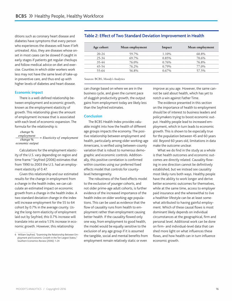
Using our preferred fixed effects model, the impact from a two standard deviation movement in the health index will give a material increase in employment. For the average county in our dataset, this equates to a 0.7-percentage point increase in the 55 to 64 population, from 56.8% to 57.5% (see Table 2).
The fixed effects methodology has the drawback of giving the same coefficient for each age cohort despite the indication of the older prime age cohorts’ increased impor-tance to the results. Because of this, the re-sults for this group are likely underestimated in Table 2. In conjunction, the impact coef-ficient on the younger age groups is likely an overestimate.
Specific health conditionsSpecific health condition impacts were
also examined using our preferred fixed ef-fect methodology. The control of between-county variation through this method is a much more rigorous test of the condition’s impact. The coefficients from this regression and a first difference regression in which the data have been z-score transformed can be found in Appendix 3.5. Of the seven condi-tions provided by age cohort in the BCBS health index dataset, impact scores from coronary heart disease, diabetes, and lipid disease have coefficients that are significant and in a consistent direction in the fixed effects and first differenced fixed effects models. Coronary heart disease and diabetes correspond to a decrease in the percent em-ployed within a county, and lipid disease has a positive correlation within counties with the percent employed of the population.
One hypothesis for this result is that people are able to work and continue rela-tively symptomless lives with lipid disease, also called high cholesterol. However, higher levels of employment allow more people to participate in yearly physicals and regular blood work. This can lead to increased detec-tion and treatment. On the other hand, con-
Table 1: Healthier People Are WorkingWithin-County Fixed Effects Model1
Panel data Observations: 16,059F(6,3005) = 35.51
Coefficient Std error T-statisticConstant 0.125 0.015 8.13z_health_score 0.033 0.015 2.21Age controls25-34 0.079 0.019 4.2035-44 -0.024 0.017 -1.3645-54 -0.079 0.017 -4.5455-64 0.033 0.025 1.2965+ -0.086 0.031 -2.76
R-squared 0.59
1Results for the 65+ age bucket are indicative of data comparability problems with the other age cohorts, caused at least in part by a majority of individuals over the age of 65 obtaining major medical services from government-sponsored Medicare rather than a private insurer such as BCBS. As such they are not representative of the popula-tion and are excluded from this discussion.
Sources: BCBS, Moody’s Analytics
BCBS �� Healthy People, Healthy Workforce
MOODY’S ANALYTICS / Copyright© 2016 16
ditions such as coronary heart disease and diabetes have symptoms that every person who experiences the diseases will have if left untreated. Also, they are diseases whose on-set in most cases can be slowed if caught in early stages if patients get regular checkups and follow medical advice on diet and exer-cise. Counties in which older workers work less may not have the same level of take-up in preventive care, and thus end up with higher levels of diabetes and heart disease.
Economic impactThere is a well-defined relationship be-
tween employment and economic growth, known as the employment elasticity of growth. This relationship gives the amount of employment increase that is associated with each level of economic expansion. The formula for the relationship is:
𝑐𝑐ℎ𝑎𝑎𝑎𝑎𝑎𝑎𝑎𝑎 % 𝑎𝑎𝑒𝑒𝑒𝑒𝑒𝑒𝑒𝑒𝑒𝑒𝑒𝑒𝑎𝑎𝑎𝑎𝑒𝑒 𝑐𝑐ℎ𝑎𝑎𝑎𝑎𝑎𝑎𝑎𝑎 %
𝑎𝑎𝑐𝑐𝑒𝑒𝑎𝑎𝑒𝑒𝑒𝑒𝑒𝑒𝑐𝑐 𝑒𝑒𝑜𝑜𝑒𝑒𝑒𝑒𝑜𝑜𝑒𝑒
= 𝐸𝐸𝑒𝑒𝑎𝑎𝐸𝐸𝑒𝑒𝑒𝑒𝑐𝑐𝑒𝑒𝑒𝑒𝑒𝑒 𝑒𝑒𝑜𝑜 𝑎𝑎𝑒𝑒𝑒𝑒𝑒𝑒𝑒𝑒𝑒𝑒𝑒𝑒𝑎𝑎𝑎𝑎𝑒𝑒
Calculations for the employment elastic-ity of the U.S. vary depending on region and time frame.6 Seyfried (2006) estimates that from 1990 to 2003 the U.S. had an employ-ment elasticity of 0.47.
Given this relationship and our estimated results for the change in employment from a change in the health index, we can cal-culate an estimated impact on economic growth from a change in the health index. A two standard deviation change in the index will increase employment for the 55 to 64 cohort by 0.7% in the average county. Us-ing the long-term elasticity of employment laid out by Seyfried, this 0.7% increase will translate into an extra 1.5% increase in eco-nomic growth. However, this relationship
6 William Seyfried, “Examining the Relationship Between Em-ployment and Economic Growth in the Ten Largest States,” Southern Economics Review (2006): 1-24
can change based on where we are in the business cycle, and given the current pace of sluggish productivity growth, the output gains from employment today are likely less than the Seyfried estimates.
ConclusionThe BCBS Health Index provides valu-
able insight into how the health of different age groups impacts the economy. The posi-tive relationship between employment and health, particularly among older working-age Americans, is verified using between-county variation that is robust to numerous demo-graphic and economic controls. Addition-ally, this positive correlation is confirmed within counties using our preferred fixed effects model that controls for county-level heterogeneity.
The robustness of the fixed effects model to the exclusion of younger cohorts, and not older prime-age adult cohorts, is further evidence of the increased importance of the health index on older working-age popula-tions. This can be used as evidence that the flow of causality runs from health to em-ployment rather than employment causing better health. If the causality flowed only one way, from employment to good health, the model would be equally sensitive to the exclusion of any age group if it is assumed the tangible, social and mental benefits from employment remain relatively static or even
improve as you age. However, the same can-not be said about health, which has yet to notch a win against Father Time.
The evidence presented in this section on the importance of health to employment should be of interest to business leaders and policymakers trying to boost economic out-put. Healthy people lead to increased em-ployment, which in turn leads to economic growth. This is shown to be especially true for the population between 45 and 60 years old. Beyond 60 years old, limitations in data make the outcome unclear.
What we do find in the study as a whole is that health outcomes and economic out-comes are directly related. Causality flow-ing in one direction cannot be definitively established, but we instead see causality most likely runs both ways. Healthy people have the ability to work longer and derive better economic outcomes for themselves, while at the same time, access to employer paid insurance and the wherewithal to live a healthier lifestyle can be at least some-what attributed to having gainful employ-ment. Which of these causal flows is most dominant likely depends on individual circumstances at the geographical, firm and personal level. Additional work can be done on firm- and individual-level data that can shed more light on what influences these flows, and how health can in turn influence economic growth.
Table 2: Effect of Two Standard Deviation Improvement in Health
Age cohort Mean employment Impact Mean employment
20-24 59.7% 1.10% 60.8%25-34 69.7% 0.85% 70.6%35-44 76.0% 0.76% 76.8%45-54 76.2% 0.79% 77.0%55-64 56.8% 0.67% 57.5%
Sources: BCBS, Moody’s Analytics
BCBS �� Healthy People, Healthy Workforce

BCBS �� Appendix
MOODY’S ANALYTICS / Copyright© 2016 17
AppendixAppendix 1.1: Selection of Controls
The association between health and out-comes for the local economy is valuable to measure in and of itself. But this does not prove that health causes those positive out-comes. Proving causality in this context is a difficult empirical task. However, if it can be shown that health and other outcomes have a statistically significant relationship even after controlling for other factors, it makes it more likely that the effect being measured is causal. Three sets of controls were derived for use in this analysis; demographic, eco-nomic and state fixed effects.
A variety of demographic factors that may be contributing to health and eco-nomic outcomes can be controlled for. The following set of county-level demographic controls were included in the regression models: percentage of the population that is white, percentage of the population that is black, percentage of the popula-tion that is Hispanic, percentage of the population that is foreign born, population density, total population, percentage of the population under age 19, percentage of the population over age 65, and share of the population that is religious. Further, a
social capital index is taken from Chetty et al that combines voter turnout, the percent of individuals who return census forms, and participation in community organizations.1
The economic controls utilized include household size, the share of children with single mothers, percentage of the population without health insurance, percentage of pop-ulation in BCBS data, share of employment in manufacturing, share of adult population with less than a high school degree, share of adult population with a college degree or more, and median household income.
Finally, state fixed effects were utilized as an additional control. This approach es-timates the models using differences from state averages for every dependent and independent variable. This means that the model uses only differences between coun-ties within the same state and avoids any potentially important omitted variables that may vary by state.
It is useful to examine whether the rela-tionship between healthcare and the local economy is robust to the inclusion of de-
1 Raj Chetty, et al. “The Association Between Income and Life Expectancy in the United States, 2001-2014,” Journal of the American Medical Association 315.16 (2016): 1750-1766.
mographic, economic and state fixed-effect controls. However, the economic controls prove problematic because they also repre-sent potential mechanisms through which health affects the economy and therefore their inclusion may bias the results toward observing no effect. For example, health may improve income by increasing educational attainment. If educational attainment is con-trolled for, then this effect of health on the economy will be missed.
In addition, some controls, such as me-dian house prices, may be so strongly related to income that they act as proxies and re-move the majority of the useful variation in income from county to county.
The tradeoff between controlling for rel-evant variables and potentially biasing the result toward observing no effect illustrates the econometric challenge of identifying the causal effect of health on the local economy.
Appendix 1.2 displays the results of the five regression models, including the base-line model with no controls. Model 4, which excludes economic controls but includes demographics and state fixed effects, is the preferred model because it likely represents the best trade-off between including relevant controls without including too many controls.

MOODY’S ANALYTICS / Copyright© 2016 18
BCBS �� Appendix
Appendix 1.2: Health ScoreModel 1 Model 2 Model 3 Model 4 Model 5
Level outcomesLog per capita income 0.178* 0.034 -0.050 0.162* 0.000Log GDP per capita 0.236*** 0.057 -0.002 0.093* 0.017Unemployment rate -0.260*** -0.065 0.031 -0.143** -0.074*% poverty -0.143* -0.022 0.037 -0.070 0.004Log avg annual pay 0.245** 0.090 0.020 0.165*** 0.094
Growth outcomesIncome per capita growth, 5 yr 0.134** 0.049 0.043 0.115*** 0.105**Income per capita growth, 10 yr 0.126* -0.004 0.036 0.109* 0.117*GDP per capita growth, 5 yr 0.120* 0.050 0.027 0.059 0.055GDP per capita growth, 10 yr 0.142* -0.017 -0.003 0.038 0.037Employment growth, 5 yr 0.162 0.112 0.079 0.215*** 0.197***Employment growth, 10 yr 0.295* 0.155 0.143** 0.286*** 0.267***Pop growth, 5 yr 0.302 0.145 0.079 0.240*** 0.179***Pop growth, 10 yr 0.343 0.250* 0.160* 0.307*** 0.247***Avg annual pay growth 0.154*** 0.064 0.060 0.098** 0.096*Avg annual pay growth 0.132** -0.009 0.003 0.052 0.053
Demographic controls X X X XEconomic controls X XState fixed effect X X
P-values: * <0.05, ** <0.01, *** <0.001.
Notes: All dependent variable and health scores standardized to z-scores. Member count is used as the regression weights, and errors are clustered at the state level. Demographic controls include % white, % black, % Hispanic, % foreign born, log population density, log population density squared, log of population, % of population ages 1 to 19, % of population aged 65 and up, social capital in-dex, % religious. Economic controls include household size, single mother % of families, % with health insurance, % of population BCBS members, % of employment in manufacturing, and log median household income.
Sources: BCBS, Moody’s Analytics

MOODY’S ANALYTICS / Copyright© 2016 19
Appendix 1.3: Mortality ScoreModel 1 Model 2 Model 3 Model 4 Model 5
Level outcomesLog per capita income -0.222** -0.082 0.088 -0.220* 0.014Log GDP per capita -0.244*** -0.079* 0.017 -0.110* -0.01Unemployment rate 0.311*** 0.07 -0.061 0.159** 0.06% poverty 0.239*** 0.041 -0.049 0.129* 0.002Log avg annual pay -0.237** -0.101* 0.012 -0.152** -0.059
Growth outcomesIncome per capita growth, 5 yr -0.106** -0.018 0.001 -0.081** -0.059Income per capita growth, 10 yr -0.098 0.027 0.012 -0.069 -0.056GDP per capita growth, 5 yr -0.100* 0.002 0.025 -0.009 0.006GDP per capita growth, 10 yr -0.135* 0.03 0.037 -0.018 0.006Employment growth, 5 yr -0.124 -0.092 -0.03 -0.179*** -0.147***Employment growth, 10 yr -0.259 -0.155 -0.092 -0.262*** -0.199***Pop growth, 5 yr -0.289 -0.176 -0.031 -0.246*** -0.128**Pop growth, 10 yr -0.351 -0.318* -0.150* -0.328*** -0.211***Avg annual pay growth -0.138*** -0.041 -0.02 -0.051 -0.035Avg annual pay growth -0.115** 0.02 0.04 -0.015 0.009
Demographic controls X X X XEconomic controls X XState fixed effects X X
P-values: * <0.05, ** <0.01, *** <0.001. Green highlights indicate statistical significance.
Notes: All dependent variable and mortality score standardized to z-scores. Member count is used as the regression weights, and errors are clustered at the state level. Demographic controls include % white, % black, % Hispanic, % foreign born, log population density, log population density squared, log of population, % of population ages 1 to 19, % of population aged 65 and up, social capital index, % religious. Economic controls include household size, single mother % of families, % with health insurance, % of population BCBS members, % of employment in manufacturing, and log median household income.
Sources: BCBS, Moody’s Analytics
BCBS �� Appendix

MOODY’S ANALYTICS / Copyright© 2016 20
Appendix 1.4: Disability ScoreModel 1 Model 2 Model 3 Model 4 Model 5
Level outcomesLog per capita income -0.144 -0.013 0.028 -0.132* -0.013Log GDP per capita -0.222*** -0.047 -0.004 -0.081 -0.019Unemployment rate 0.228*** 0.056 -0.02 0.123** 0.071*% poverty 0.088 0.007 -0.032 0.037 -0.009Log avg annual pay -0.235** -0.083 -0.034 -0.162*** -0.104*
Growth outcomesIncome per capita growth, 5 yr -0.148** -0.064 -0.062 -0.127*** -0.122**Income per capita growth, 10 yr -0.139* -0.008 -0.058 -0.124** -0.139*GDP per capita growth, 5 yr -0.131* -0.073 -0.05 -0.078 -0.078GDP per capita growth, 10 yr -0.144* 0.008 -0.013 -0.047 -0.055Employment growth, 5 yr -0.18 -0.119* -0.099* -0.223*** -0.212***Employment growth, 10 yr -0.307* -0.147 -0.160** -0.281*** -0.282***Pop growth, 5 yr -0.3 -0.124 -0.096 -0.221*** -0.188***Pop growth, 10 yr -0.332 -0.211 -0.159* -0.279*** -0.248***Avg annual pay growth -0.160*** -0.072* -0.073* -0.111** -0.113**Avg annual pay growth -0.137** 0.005 -0.019 -0.064 -0.075
Demographic controls X X X XEconomic controls X XState fixed effects X X
P-values: * <0.05, ** <0.01, *** <0.001. Green highlights indicate statistical significance.
Notes: All dependent variable and disability score standardized to z-scores. Member count is used as the regression weights, and errors are clustered at the state level. Demographic controls include % white, % black, % Hispanic, % foreign born, log population density, log population density squared, log of population, % of population ages 1 to 19, % of population aged 65 and up, social capital index, % religious. Economic controls include household size, single mother % of families, % with health insurance, % of population BCBS members, % of employment in manufacturing, and log median household income.
Sources: BCBS, Moody’s Analytics
BCBS �� Appendix

MOODY’S ANALYTICS / Copyright© 2016 21
Appendix 1.5: Specific Condition Regressions, Model 1No controls
Impact score PrevalenceCondition coefficient p-value coefficient p-valueBH - alcohol / substance abuse -0.174 0.087 -0.562 0.000BH - depression / anxiety / affective ds 0.486 0.000 0.045 0.651CV - hypertension -0.600 0.000 -0.673 0.000Endo - lipid ds -0.303 0.007 -0.245 0.023Endo - DM -0.466 0.000 -0.325 0.003BH - psychotic ds 0.704 0.000 0.632 0.000CV - coronary ds -0.507 0.000 -0.399 0.000BH - hyperactivity / related 0.387 0.000 0.460 0.000GI - regional enteritis / ulcerative colitis 0.617 0.000 0.631 0.000Resp - COPD -0.773 0.000 -0.690 0.000Immune sys- rheumatoid arthr/related -0.442 0.004 -0.428 0.001Endo - hypothyroidism -0.011 0.945 -0.018 0.896Cancer - breast 0.631 0.000 0.422 0.001Resp - asthma 0.546 0.000 0.500 0.000CV - heart failure / cardiomyopathy -0.270 0.034 -0.256 0.035CV - valve dysfunction -0.075 0.226 -0.029 0.584GU - renal failure -0.136 0.299 -0.135 0.058MS - spine / neck / back -0.268 0.061 -0.313 0.026NS - epilepsy / convulsions -0.106 0.233 -0.169 0.129Eye - visual impairment / blindness 0.074 0.578 0.108 0.390Cancer - leukemia / lymphoma / myeloma 0.471 0.004 0.610 0.001BH - dementia / related 0.267 0.093 0.318 0.010NS - cerebrovascular ds / stroke -0.150 0.337 -0.138 0.134NS - multiple sclerosis 0.377 0.022 0.389 0.004GI - cirrhosis / sequelae -0.182 0.135 -0.132 0.055
Notes: All dependent variable and health scores standardized to z-scores. Member count is used as the re-gression weights, and errors are clustered at the state level. Model includes demographic controls and state fixed effects. Statistically significant, negative associationStatistically significant, positive associationSources: BCBS, Moody’s Analytics
BCBS �� Appendix
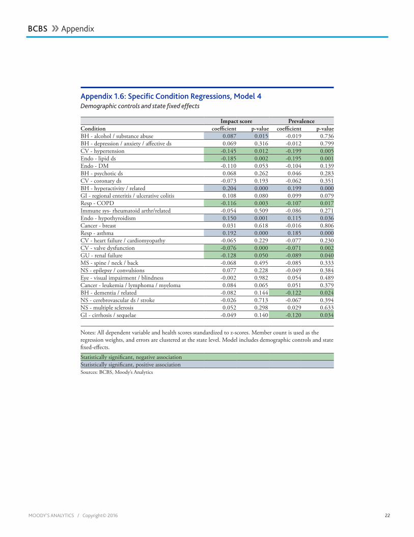
MOODY’S ANALYTICS / Copyright© 2016 22
Appendix 1.6: Specific Condition Regressions, Model 4Demographic controls and state fixed effects
Impact score PrevalenceCondition coefficient p-value coefficient p-valueBH - alcohol / substance abuse 0.087 0.015 -0.019 0.736BH - depression / anxiety / affective ds 0.069 0.316 -0.012 0.799CV - hypertension -0.145 0.012 -0.199 0.005Endo - lipid ds -0.185 0.002 -0.195 0.001Endo - DM -0.110 0.053 -0.104 0.139BH - psychotic ds 0.068 0.262 0.046 0.283CV - coronary ds -0.073 0.193 -0.062 0.351BH - hyperactivity / related 0.204 0.000 0.199 0.000GI - regional enteritis / ulcerative colitis 0.108 0.080 0.099 0.079Resp - COPD -0.116 0.003 -0.107 0.017Immune sys- rheumatoid arthr/related -0.054 0.509 -0.086 0.271Endo - hypothyroidism 0.150 0.001 0.115 0.036Cancer - breast 0.031 0.618 -0.016 0.806Resp - asthma 0.192 0.000 0.185 0.000CV - heart failure / cardiomyopathy -0.065 0.229 -0.077 0.230CV - valve dysfunction -0.076 0.000 -0.071 0.002GU - renal failure -0.128 0.050 -0.089 0.040MS - spine / neck / back -0.068 0.495 -0.085 0.333NS - epilepsy / convulsions 0.077 0.228 -0.049 0.384Eye - visual impairment / blindness -0.002 0.982 0.054 0.489Cancer - leukemia / lymphoma / myeloma 0.084 0.065 0.051 0.379BH - dementia / related -0.082 0.144 -0.122 0.024NS - cerebrovascular ds / stroke -0.026 0.713 -0.067 0.394NS - multiple sclerosis 0.052 0.298 0.029 0.633GI - cirrhosis / sequelae -0.049 0.140 -0.120 0.034
Notes: All dependent variable and health scores standardized to z-scores. Member count is used as the regression weights, and errors are clustered at the state level. Model includes demographic controls and state fixed-effects.
Statistically significant, negative associationStatistically significant, positive associationSources: BCBS, Moody’s Analytics
BCBS �� Appendix

MOODY’S ANALYTICS / Copyright© 2016 23
BCBS �� Appendix
Appendix 3.1: Selection of Controls
The association between health and employment for the local economy does not in and of itself prove that health causes employment at different ages. Indeed, prov-ing causality in this context is a difficult em-pirical task. However, if it can be shown that health and employment have a statistically significant relationship even after controlling for other factors, it makes it more likely that the effect being measured is causal. Three sets of controls were derived for use in this analysis; demographic, economic, and state fixed effects.
A variety of demographic factors can be controlled for that may be contributing to both health and employment outcomes. The following set of county-level demographic
controls were included in the regression models: percentage of the population that is white, percentage of the population that is black, percentage of the population that is Hispanic, percentage of the population that is foreign born, population density, total population, percentage of the population under age 19, percentage of the population over age 65, and share of the population that is religious. Further, a social capital index is taken from Chetty et al. that combines voter turnout, the percent of individuals who re-turn census forms, and participation in com-munity organizations.1
1 Raj Chetty, et al., “The Association Between Income and Life Expectancy in the United States, 2001-2014,” Journal of the American Medical As-sociation 315.16 (2016): 1750-1766.
The economic controls utilized include percent of the population without health insurance, share of adult population with a college degree or more, and median house value.
Finally, state fixed effects were utilized as an additional control. This approach es-timates the models using differences from state averages for every dependent and independent variable. This means that the model uses only differences between coun-ties within the same state and avoids any potentially important omitted variables that may vary by state.
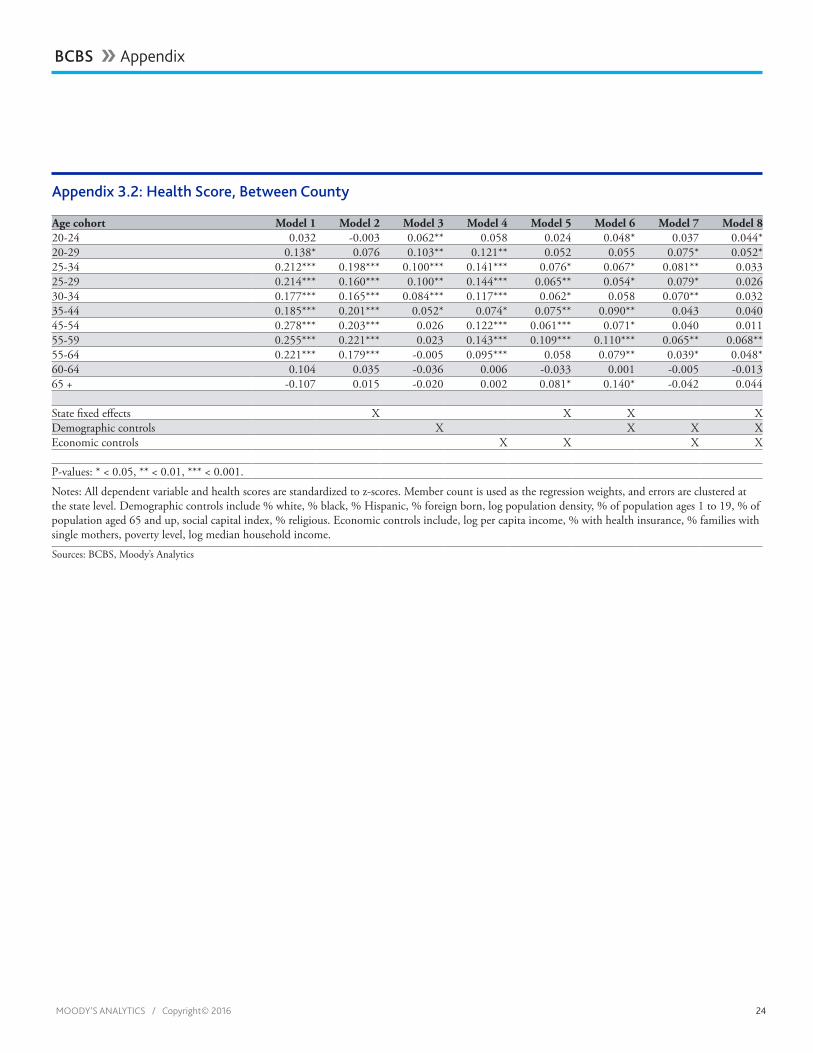
MOODY’S ANALYTICS / Copyright© 2016 24
Appendix 3.2: Health Score, Between County
Age cohort Model 1 Model 2 Model 3 Model 4 Model 5 Model 6 Model 7 Model 820-24 0.032 -0.003 0.062** 0.058 0.024 0.048* 0.037 0.044*20-29 0.138* 0.076 0.103** 0.121** 0.052 0.055 0.075* 0.052*25-34 0.212*** 0.198*** 0.100*** 0.141*** 0.076* 0.067* 0.081** 0.03325-29 0.214*** 0.160*** 0.100** 0.144*** 0.065** 0.054* 0.079* 0.02630-34 0.177*** 0.165*** 0.084*** 0.117*** 0.062* 0.058 0.070** 0.03235-44 0.185*** 0.201*** 0.052* 0.074* 0.075** 0.090** 0.043 0.04045-54 0.278*** 0.203*** 0.026 0.122*** 0.061*** 0.071* 0.040 0.01155-59 0.255*** 0.221*** 0.023 0.143*** 0.109*** 0.110*** 0.065** 0.068**55-64 0.221*** 0.179*** -0.005 0.095*** 0.058 0.079** 0.039* 0.048*60-64 0.104 0.035 -0.036 0.006 -0.033 0.001 -0.005 -0.01365 + -0.107 0.015 -0.020 0.002 0.081* 0.140* -0.042 0.044
State fixed effects X X X XDemographic controls X X X XEconomic controls X X X X
P-values: * < 0.05, ** < 0.01, *** < 0.001.
Notes: All dependent variable and health scores are standardized to z-scores. Member count is used as the regression weights, and errors are clustered at the state level. Demographic controls include % white, % black, % Hispanic, % foreign born, log population density, % of population ages 1 to 19, % of population aged 65 and up, social capital index, % religious. Economic controls include, log per capita income, % with health insurance, % families with single mothers, poverty level, log median household income.
Sources: BCBS, Moody’s Analytics
BCBS �� Appendix

MOODY’S ANALYTICS / Copyright© 2016 25
Appendix 3.3: Within-County First Difference Fixed Effects Model Panel data Observations: 12,145F(6,3005) = 35.51
Coefficient Std Error T-statisticConstant 0.069 0.016 4.39D.z_percent_employed 0.122 0.122 0.122Age controls35-44 -0.177 0.032 -5.5945-54 -0.120 0.023 -5.1355-64 0.040 0.021 1.8865+ -0.171 0.025 -6.88
R-squared 0.18
Notes: All dependent variable and health scores are standardized to z-scores. Member count is used as the regression weights, and errors are clustered at the county level. Model includes county-level fixed effects.
Sources: BCBS, Moody’s Analytics
BCBS �� Appendix

MOODY’S ANALYTICS / Copyright© 2016 26
Appendix 3.4: Age-Specific Robustness Check, Within-County Fixed Effects ModelAge cohort controls and constant included
Age cohort withheld from model Coefficient20-24 0.02125-34 0.01735-44 0.01645-54 0.01655-64 0.01965+ 0.031Statistically significant 5%Statistically significant 1%
Notes: All dependent variable and health scores are standardized to z-scores. Member count is used as the regression weights, and errors are clustered at the county level. Model includes county-level fixed effects. Sources: BCBS, Moody’s Analytics
BCBS �� Appendix

MOODY’S ANALYTICS / Copyright© 2016 27
Appendix 3.5: Specific Condition Regressions, Model 4Demographic controls and state fixed effects
Impact score Impact scoreFixed effect model First difference model
Condition Coefficient p-value Coefficient p-valueBH - alcohol / substance abuse 0.02 0.08 -0.05 0.00BH - depression / anxiety / affective ds -0.02 0.15 -0.05 0.00CV - hypertension -0.02 0.26 -0.09 0.00Endo - lipid ds 0.06 0.00 0.01 0.21Endo - DM -0.06 0.00 -0.08 0.00CV - coronary ds -0.03 0.02 -0.05 0.00NS - multiple sclerosis 0.01 0.57 -0.03 0.09
Preferred model statistically significant, 5%Coefficients in same directionNotes: All dependent variable and health scores are standardized to z-scores. Member count is used as the regression weights, and errors are clustered at the county level. Model includes county-level fixed effects. Sources: BCBS, Moody’s Analytics
BCBS �� Appendix

About Moody’s Analytics
Moody’s Analytics helps capital markets and credit risk management professionals worldwide respond to an evolving
marketplace with confi dence. With its team of economists, the company offers unique tools and best practices for
measuring and managing risk through expertise and experience in credit analysis, economic research, and fi nancial
risk management. By offering leading-edge software and advisory services, as well as the proprietary credit research
produced by Moody’s Investors Service, Moody’s Analytics integrates and customizes its offerings to address specifi c
business challenges.
Concise and timely economic research by Moody’s Analytics supports fi rms and policymakers in strategic planning, product and sales forecasting, credit risk and sensitivity management, and investment research. Our economic research publications provide in-depth analysis of the global economy, including the U.S. and all of its state and metropolitan areas, all European countries and their subnational areas, Asia, and the Americas. We track and forecast economic growth and cover specialized topics such as labor markets, housing, consumer spending and credit, output and income, mortgage activity, demographics, central bank behavior, and prices. We also provide real-time monitoring of macroeconomic indicators and analysis on timely topics such as monetary policy and sovereign risk. Our clients include multinational corporations, governments at all levels, central banks, fi nancial regulators, retailers, mutual funds, fi nancial institutions, utilities, residential and commercial real estate fi rms, insurance companies, and professional investors.
Moody’s Analytics added the economic forecasting fi rm Economy.com to its portfolio in 2005. This unit is based in West Chester PA, a suburb of Philadelphia, with offi ces in London, Prague and Sydney. More information is available at www.economy.com.
Moody’s Analytics is a subsidiary of Moody’s Corporation (NYSE: MCO). Further information is available at www.moodysanalytics.com.
About Moody’s Corporation
Moody’s is an essential component of the global capital markets, providing credit ratings, research, tools and analysis that contribute to transparent and integrated fi nancial markets. Moody’s Corporation (NYSE: MCO) is the parent company of Moody’s Investors Service, which provides credit ratings and research covering debt instruments and securities, and Moody’s Analytics, which encompasses the growing array of Moody’s nonratings businesses, including risk management software for fi nancial institutions, quantitative credit analysis tools, economic research and data services, data and analytical tools for the structured fi nance market, and training and other professional services. The corporation, which reported revenue of $3.5 billion in 2015, employs approximately 10,400 people worldwide and maintains a presence in 36 countries.
© 2016, Moody’s Analytics Inc. and/or its licensors and affi liates (together, “Moody’s”). All rights reserved. ALL INFORMATION CONTAINED HEREIN IS PROTECTED BY COPYRIGHT LAW AND NONE OF SUCH INFORMATION MAY BE COPIED OR OTHERWISE REPRODUCED, REPACKAGED, FURTHER TRANSMITTED, TRANSFERRED, DISSEMINATED, REDISTRIBUTED OR RESOLD, OR STORED FOR SUBSEQUENT USE FOR ANY PURPOSE, IN WHOLE OR IN PART, IN ANY FORM OR MANNER OR BY ANY MEANS WHATSOEVER, BY ANY PERSON WITHOUT MOODY’S PRIOR WRITTEN CONSENT. All information contained herein is obtained by Moody’s from sources believed by it to be accurate and reliable. Because of the possibility of human and mechanical error as well as other factors, however, all information contained herein is provided “AS IS” without warranty of any kind. Under no circumstances shall Moody’s have any liability to any person or entity for (a) any loss or damage in whole or in part caused by, resulting from, or relating to, any error (negligent or otherwise) or other circumstance or contingency within or outside the control of Moody’s or any of its directors, offi cers, employees or agents in connection with the procurement, collection, compilation, analysis, interpretation, communication, publication or delivery of any such information, or (b) any direct, indirect, special, consequential, compensatory or incidental damages whatsoever (including without limitation, lost profi ts), even if Moody’s is advised in advance of the possibility of such damages, resulting from the use of or inability to use, any such information. The fi nancial reporting, analysis, projections, observations, and other information contained herein are, and must be construed solely as, statements of opinion and not statements of fact or recommendations to purchase, sell, or hold any securities. NO WARRANTY, EXPRESS OR IMPLIED, AS TO THE ACCURACY, TIMELINESS, COMPLETENESS, MERCHANTABILITY OR FITNESS FOR ANY PARTICULAR PURPOSE OF ANY SUCH OPINION OR INFORMATION IS GIVEN OR MADE BY MOODY’S IN ANY FORM OR MANNER WHATSOEVER. Each opinion must be weighed solely as one factor in any investment decision made by or on behalf of any user of the information contained herein, and each such user must accordingly make its own study and evaluation prior to investing.

This is the eleventh study of the Blue Cross Blue Shield: The Health of America Report series, a collaboration between BCBSA and Blue Health Intelligence, which uses a market-leading claims database to uncover key trends and insights into
health care affordability and access to care.
Blue Cross Blue Shield Health IndexSM Methodology
The Blue Cross Blue Shield Health IndexSM is a unique measurement of the state of America’s health powered by data from more than 40 million of our members. This first-of-its-kind resource identifies the health conditions with the greatest impact on commercially-insured Americans.
The BCBS Health Index is informed by data from Blue Cross Blue Shield Axis®, the BCBS companies’ industry-leading data capability. It is also a result of collaboration with Blue Health Intelligence®, which provided analytical support, and consultation with the Institute for Health Metrics and Evaluation, an independent global health research center at the University of Washington in Seattle, that helped BCBS in defining condition categories and measuring their disabling affects.
Using blinded claims data from more than 40 million commercially insured members of BCBS companies, ICD-9 diagnoses were mapped to over 200 health condition categories. The impact of each condition was determined based on the years lost due to the risk of premature death and the disabling effects of illness or disease. These years of life lost were subtracted from the optimum life expectancy (OLE) of a given member assuming no health conditions and then divided by OLE to get an estimate of health between 0 and 1 with 1 corresponding to optimal health, defined as the absence of any currently known conditions or risks associated with potential adverse health impacts. A value less than one represents the proportion of future healthy life for that member based on his or her diagnosed condition(s). These individual level estimates are then aggregated to create a health score for the population.
The formal calculation is [OLE – (Mortality + Disability)] / OLE, where “OLE” is a person’s optimum life expectancy derived from an actuarial life table, “mortality” is “years of life lost” due to risk of premature death, and “disability” is years of living with a disability.
BLUE CROSS BLUE SHIELD, THE HEALTH OF AMERICA REPORT