health and labor

1

Health and Labor Supply; A Simultaneous Equation Model Approach Maryam Jafari Bidgoli1

Abstract. Using the RAND HRS panel data (1996-2010), we examine the relationship between health and

labor supply. Employing a simultaneous equation model allows for treating health as endogenous to labor

supply. People might report poor health to justify their non-employment status; therefore the effect of health

may be overestimated. The results confirm that health has a positive and significant effect on labor supply

for both males and females. The effect of labor supply on health is also positive and significant. We also

examine the impact of health insurance coverage on both labor supply and health. To address the possible

endogeneity of health insurance coverage to labor supply, we rerun the model for a group of married males

and females who have health insurance through their spouses’ employers. The finding indicates that health

insurance has a statistically significant effect on labor supply for both males and females.

1. Introduction

The amount of time a person can spend producing earnings depends on his/her stock of health

as a durable human capital stock. Individuals’ initial health stock depreciates with age (Grossman,

1972). Health is generally considered as an important determinant of individuals’ labor supply. Poor

health may affect time allocation between leisure and work, and reduce the total amount of time

available to spend on the labor market. Impaired health is a major cause of non-employment in middle

age and older, and it is a significant constraint on the earning capacity and employment opportunities

of aging populations (García-Gómez, Kippersluis, O’Donnell, & Doorslaer, 2013). According to the

World Health Organization (WHO), chronic diseases are a major cause of mortality globally, and have

significant effects on people’s physical activities. We cannot neglect the economic burden of chronic

diseases on individuals’ lives in terms of non-employment and early retirement. Simultaneously,

technological advances in medical treatments have caused people to live longer. The advances also

effect function and quality of life of those with diseases. Therefore, individuals suffering from chronic

1 PhD candidate, Department of Economics, Wayne State University Email [email protected] Tel. +1(248) 824 5127

2

diseases are now more likely to remain in the labor market. Evaluating the economic and social burdens

of such health impairments is essential.

2. Background

Many studies have focused on the linkage between poor health and labor market outcomes. The

impact of impaired health on labor supply has previously been analyzed using various proxies for poor

health. Others research has focused instead on the effect of labor outcomes, such as wage and hours of

work, on health. Few studies have considered health as an endogenous variable and simultaneously

determined the effect of health on labor supply and vice versa.

Many studies have treated health as an exogenous variable, and used different ways to measure

and include health in the labor supply equation. Some of them included health in the labor supply

equation using a discrete self-reported health status (poor, fair, good, very good, and excellent) variable.

Others have narrowed their focus to a specific disease such as arthritis or cancer, or have focused on

disability (Bradley, et al. 2002; Jean and Burkhauser, 1990; Bradley et al, 2005; Stern, 1989). Jean and

Burkhauser (1990) studied the effect of poor health on both wage rates and hours of work. They used a

simultaneous Tobit model for hourly wage and hours worked to examine the impact of arthritis on

wages and hours of work. They argue that arthritis ideal for studying the effect of poor health on labor

market activities in the sense that it is the most common chronic disease and also the second leading

cause of work disability in the US. They found that the total wage earnings of those suffering from

arthritis are significantly below those of healthy workers. Neumark, et al (2002) examined the effect of

breast cancer on women’s labor supply. They estimated the probability of working for a group of

women who have had breast cancer. They found that the probability of working is 10 percentage points

lower for breast cancer survivors than women without cancer.

If (reported) health is endogenous with respect to labor supply, then including health as an

exogenous factor in modeling labor supply will cause the estimated effect to be biased. Few researches

(Stern 1989; Cai and Kalb 2006; Cai 2010) have tried to address the potential endogeneity of health in

the labor supply equation. When the measure of health is based on respondents’ self-reports, researchers

are more concerned about this bias than when more objective health measures are used. For example,

3

some people may underrate their health to justify their non-employment status. Thus, including health

as an exogenous variable may result in an upward biased effect of health on labor supply.

The endogeneity of health has been addressed by measuring health differently or by using

different econometric approaches. Lee (1982) examined the relationship between health and wage using

a structural equations model. Lee found that the wage rate coefficient in the health equation is

significantly positive, and also that the health coefficient in the wage equation is significantly positive.

After correcting for measurement error in self-reported health , the effect of health on wage is still

strong and positive, but about 28 percent lower then the uncorrected estimate. He concluded that wages

and health capital are significantly jointly determined.

Using a simultaneous equations model of labor force participation and endogenous self-

reported disability, Stern (1989) found that participation is statistically insignificant in the disability

equation, and that disability measures are all statistically significant in the labor force participation

equationHe addresses two potential sources of disability endogeneity: a direct effect of participation on

disability, such as the effect of poor working conditions, and errors in self-reports of disability. Cai and

Kalb (2006) follow Stern’s approach. Using simultaneous equations of health and labor force

participation, they estimate the effect of self-assessed health on participation. They find health to be

endogenous in the labor force participation equation. In a separate study, Cai (2010) used Australian

panel datato estimate the effect of health on labor force participation using the same method. His

findings showed that health has a positive and significant effect on labor force participation, and that

labor force participation has a negative effect on health for males, but a positive effect on health for

females.

Among the studies focused on specific chronic conditions, most treated the incidence of chronic

diseases as exogenous (Bradley, et al. 2013; Bradley, et al. 2012; Bradley et al. 2007; Bradley et al.

2005). Zhang, et al (2009) examined the effect of health on labor force participation by including the

incidence of chronic diseases. Their finding rejected exogeneity of chronic diseases. Nevertheless, it

has been argued that use of specific chronic conditions reduces the potential measurement error as

compared to using self-reported health status.

4

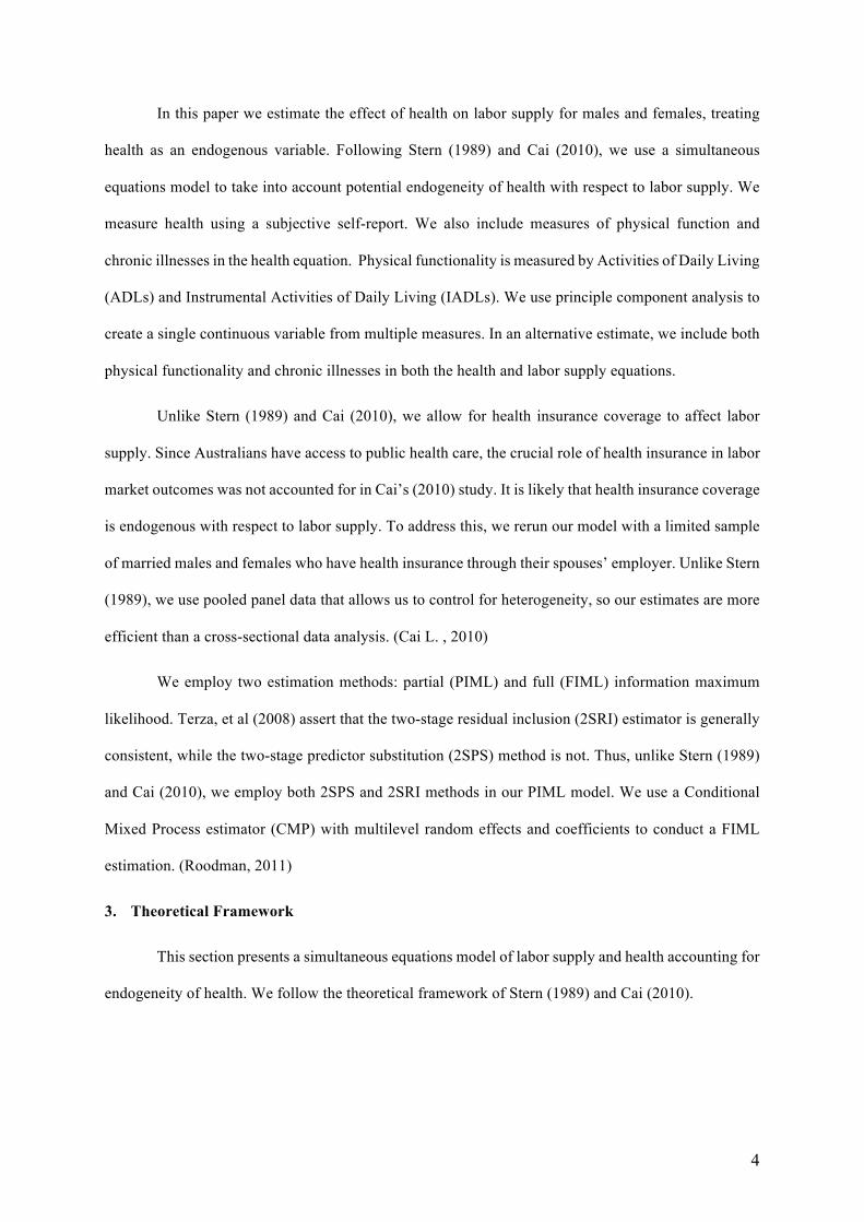
In this paper we estimate the effect of health on labor supply for males and females, treating

health as an endogenous variable. Following Stern (1989) and Cai (2010), we use a simultaneous

equations model to take into account potential endogeneity of health with respect to labor supply. We

measure health using a subjective self-report. We also include measures of physical function and

chronic illnesses in the health equation. Physical functionality is measured by Activities of Daily Living

(ADLs) and Instrumental Activities of Daily Living (IADLs). We use principle component analysis to

create a single continuous variable from multiple measures. In an alternative estimate, we include both

physical functionality and chronic illnesses in both the health and labor supply equations.

Unlike Stern (1989) and Cai (2010), we allow for health insurance coverage to affect labor

supply. Since Australians have access to public health care, the crucial role of health insurance in labor

market outcomes was not accounted for in Cai’s (2010) study. It is likely that health insurance coverage

is endogenous with respect to labor supply. To address this, we rerun our model with a limited sample

of married males and females who have health insurance through their spouses’ employer. Unlike Stern

(1989), we use pooled panel data that allows us to control for heterogeneity, so our estimates are more

efficient than a cross-sectional data analysis. (Cai L. , 2010)

We employ two estimation methods: partial (PIML) and full (FIML) information maximum

likelihood. Terza, et al (2008) assert that the two-stage residual inclusion (2SRI) estimator is generally

consistent, while the two-stage predictor substitution (2SPS) method is not. Thus, unlike Stern (1989)

and Cai (2010), we employ both 2SPS and 2SRI methods in our PIML model. We use a Conditional

Mixed Process estimator (CMP) with multilevel random effects and coefficients to conduct a FIML

estimation. (Roodman, 2011)

3. Theoretical Framework

This section presents a simultaneous equations model of labor supply and health accounting for

endogeneity of health. We follow the theoretical framework of Stern (1989) and Cai (2010).

5

The variation in the value of Labor Supply (LS) can be estimated by the variation intrue (but

unmeasured) health, and a set of exogenous variables. The first equation specifies the determination of

labor supply.

(Labor Supply). = γ1 True health + (Exogenous vars)1,.φ1 + (e)1,. Eq. 1

𝛾@ and 𝜑@ are coefficients to be estimated.

The second equation specifies latent (true) health as a function of labor supply and a set of exogenous

variables.

(True health). = γB(Labor supply). + (Exogenous vars)B,.φB + (e)B,. Eq. 2

The true value of health is unobservable. Thus, we need another equation that presents the

relationship between true health and observable health measures, such as self-reported health scores.

The third equation represents the observed (self-reported) health status as a function of the true value

of health and labor supply. The dependency of self-reported health status indicates the endogeneity of

self-reported health. A positive γB would imply that those working for pay tend to overstate their health

and those not working tend to understate their health.

(Observed health).=(True health). + γB(Labor supply). + (e)E,. Eq. 3

Three error terms are assumed to be jointly normally distributed.

By substituting Eq. (2) into Eqs. (1) and (3), we obtain Eqs. (4) and (5).

(𝑂𝑏𝑠𝑒𝑟𝑣𝑒𝑑 ℎ𝑒𝑎𝑙𝑡ℎ)Q = 𝜃S(𝐿𝑎𝑏𝑜𝑟 𝑠𝑢𝑝𝑝𝑙𝑦)Q + 𝑒𝑥𝑜𝑔𝑒𝑛𝑜𝑢𝑠 𝑣𝑎𝑟𝑠 S,Q𝜑S+(𝑒)S,Q Eq. 4

𝑤ℎ𝑒𝑟𝑒 𝜃S = 𝛾S + 𝛾@

𝑙𝑎𝑏𝑜𝑟 𝑠𝑢𝑝𝑝𝑙𝑦 Q =]^

_`]^]a𝑂𝑏𝑠𝑒𝑟𝑣𝑒𝑑 ℎ𝑒𝑎𝑙𝑡ℎ Q+ 𝐸𝑥𝑜𝑔𝑒𝑛𝑜𝑢𝑠 𝑣𝑎𝑟𝑠 @Q

c^_`]^]a

+ 𝑒 @,Q Eq. 5

𝑤ℎ𝑒𝑟𝑒 ]^_`]^]a

= 𝜃@ and c^_`]^]a

= 𝜑@

𝜃S is a coefficient to be estimated.

In many surveys, including the HRS, respondents are asked to rate their health from poor to

excellent; poor (=1), fair (=2), good (=3), very good (=4), and excellent (=5). Thus, the observed

endogenous health variable is:

6

H=κ if mh < unobserved health ≤ mk where k = 1,2,3,4, and 5 Eq. 6

𝑤ℎ𝑒𝑟𝑒 𝑖 = −1, 0, 1, 2, 𝑎𝑛𝑑 3 , 𝑚w_ = −∞ 𝑎𝑛𝑑 ( 𝑗 = 0, 1, 2,3 𝑎𝑛𝑑 4 , 𝑚z = +∞)

We observe self-reported health status, but not cut-off points in an underlying continuous observed

health measure, which are coefficients to be estimated.

The endogenous labor supply variable is:

L. =1 = 𝑤𝑜𝑟𝑘𝑖𝑛𝑔 𝑓𝑜𝑟 𝑝𝑎𝑦 0 (= 𝑛𝑜𝑡 𝑤𝑜𝑟𝑘𝑖𝑛𝑔 𝑓𝑜𝑟 𝑝𝑎𝑦)

Eq. 7

Equations 4 to 7 are used to construct a simultaneous equations model. 𝜃S, 𝜑S, 𝜃@, 𝑎𝑛𝑑 𝜑@ are

coefficients to be estimated. In addition, 𝑚},𝑚_,𝑚~, 𝑎𝑛𝑑 𝑚� are health cut-off points to be estimated.

The modeling approach is similar to Stern (1989), who estimated the model using cross

sectional US data, and Cai (2010), who uses Australian longitudinal data. We follow their method to

estimate the effect of endogenous health on labor supply. We use both the two-stage predictor

substitution (2SPS), and two-stage residual inclusion (2SRI) methods. As Terza, et al (2008) argued,

the 2SRI estimator is generally consistent while the 2SPS method is not. The 2SRI approach was first

discussed by Hausman (1978), and developed further by Smith and Blundell (1986). The 2SRI method,

instead of including the predicted value of an endogenous variable from the first stage in the second

stage, includes the residual of the first stage in the second stage, while also including the observable

endogenous variable as a regressor in the second stage. Terza, et al (2008) also argue that, like two-

stage least squares (2SLS) for linear models, the 2SPS approach for nonlinear models is not consistent.

The 2SRI method addresses this limitation.

4. Variables

Figure 1 illustrates the relationship between health and labor supply as endogenous variables,

and their dependence on other exogenous and control variables.

7

Figure 1. reciprocal causation

In this model, X1 and X2 are considered endogenous variables, which are determined in the

model simultaneously. X3, X4, and X5 are sets of exogenous variables that are determined outside the

model. u and v are the residuals and are correlated. The arrows from X4 to X5 and from X5 to X4

indicate the endogeneity of health and employment status.

Exclusion restrictions are required to identify the simultaneous equation model. The following

paragraphs illustrate the included and excluded variables in each equation of the model, and provide

definitions of the variables.

X1, Labor supply is defined as a binary variable that equals one if the respondent reports

currently working for pay.

X2, Health status is the respondent’s self-reported general health status, scaled from “1” for

poor to “5” for excellent.

X3, is a set of exogenous variables included in the health equation and excluded from the labor

supply equation: Chronic conditions, physical functionality, health insurance, and current preventive

behaviors are the included variables in the health equation. The chronic conditions are high blood

pressure, diabetes, cancer, lung disease, heart disease, stroke, psychiatric problems, and arthritis.

Respondents were asked whether or not a doctor told the respondent he/she had each condition. We use

ADLs (five tasks of bathing, eating, dressing, walking across a room, and getting in or out of bed) and

IADLs (using a telephone, talking meditation, handling money, shopping, preparing meals) to construct

a physical functionality variable. Following (Ginneken & Groenewold, 2012), we use principle

X3: Chronic conditions, No. of chronic conditions., Physical functionality, Health insurance, Current

and lagged smoker, Current and lagged heavy drinker, and lagged preventive behaviors

X2: Health u: Unobservable variables

X4: Age, Age squared, Age 62+, marital status, level of education, types of occupation and

household wealth

X5: Child under 18, Married*Child under 18, Employer provided health insurance, Levels of

education*Age 62+, and Year dummies X1: Labor Supply v: Unobservable variables

8

component analysis (PCA) of 10 items to create a single index of physical functionality. The first

component explains the most of the variance. PCA results are reported in the Appendix. As Cai (2010)

argues, chronic health conditions and physical functioning may be treated as exogenous variables.

Although these are also reported by the respondents, they are more objective. It is difficult to estimate

the effect of health insurance on health because the same determinants are expected to influence both

health and health insurance coverage. In addition, health status may directly affect insurance coverage

(Levy & Meltzer, 2008).

X4, is a set of variables that affects both health and labor supply. Age, age squared, marital

status (married versus unmarried), level of education (less than high school completion, high school,

some college, college degree, more than college), type of occupation (white collar 1, white collar 2,

and blue collar)2, household wealth3, current smoker, current heavy drinker4, and lagged preventive

behaviors5. The potential wage is also a factor that influences both health and labor supply equations.

We include level of education, type of occupation, age, and age squared as proxies for the potential

wage in both equations.

X5, is a set of variables that are included in the labor equation and excluded from the health

equation. Having a young child residing with the respondent is an obstacle to labor supply. The

interaction between the presence of a resident child and marital status is also included in the labor

supply equation. As previous studies argue, employer-provided health insurance is endogenous to the

labor supply (Bradley, Neumark, & Barkowski, 2013; Bradley, Neumark, & Motika, 2012). . In order

to take the endogeneity of the employer-provided health insurance into account, we rerun the model

for a group of married individuals who have health insurance through their spouse. The number of

chronic conditions and year dummies are also included in the labor supply equation.

2 White collar 1 includes managerial specialty operation or technical support, white collar 2 includes sales, clerical, administrative support or services, and blue collar includes farming, forestry, fishing, mechanics and repair, construction trade and extractors, precision production or operators 3 The net value of total wealth (excluding second home) is calculated as the sum of all wealth components less all debt

4 According to National Institute on Alcohol Abuse and Alcoholism, Heavy drinking defines as drinking 5 or more drinks on the same occasion on each of 5 or more days in the past 30 days. We define a heavy drinker as a person who drinks more than 5 standards drinks a day when drinking or drinks five days a week. 5 The preventive behavior is defined as whether the respondent reports preventive health tests and procedures such as a blood test for cholesterol, a flu shot, monthly self-checks for breast lumps, a mammogram, a pap smear, and a check for prostate cancer.

9

5. Econometric Approach

5.1. Two-Stage method

We employ a two-step nonlinear estimator to estimate health and employment status, allowing for

endogeneity of these variables. The reduced forms for Eq. (6) and Eq. (7) are as follows:

E . = ΧΠ1 + e 1 Eq. 8

(H). = ΧΠB + e B Eq. 9

We estimate Π1 and ΠB using two instrumental variables based approaches: two-stage predictor

substitution (2SPS), and two-stage residual inclusion (2SRI). We compute the predicted value of

employment status using a random effects probit model, and the predicted value of health using an

ordered probit model.

Under the 2SPS method, we regress endogenous variables on all exogenous variables and covariates in

the first stageand obtain the predicted value of endogenous variable. In the second stage, this predicted

value replaces the observed value (Stern 1989; Terza, Basu, & Rathouz 2008; Cai, Small, & Ten Have,

2011). The disadvantage of this method is that the correlation between the two equations is not taken

into account (Cai L. , 2010). Π1 is estimated using a probit model for panel data , and ΠB is estimated

using ordered probit. Then we have Eq. 10 and Eq. 11.

𝐸 . = ΧΠ1 Eq. 10

𝐻 . = ΧΠS Eq. 11

In the second-stage , we substitute Π1and ΠB in Eq.8 and Eq. 9.

(Terza, Basu, & Rathouz, 2008) demonstrated the superiority of the 2SRI method to the 2SPS

method when trying to address endogeneity in nonlinear models. In the 2SRI approach, the first-stage

is identical to the 2SPS. However, instead of using the predicted value of endogenous variable from the

first-stage regression in the second-stage regression, we use both the observable endogenous variable

and the first-stage residuals as regressors in the second-stage estimation. We define the residuals in the

model as Eq. 12.

10

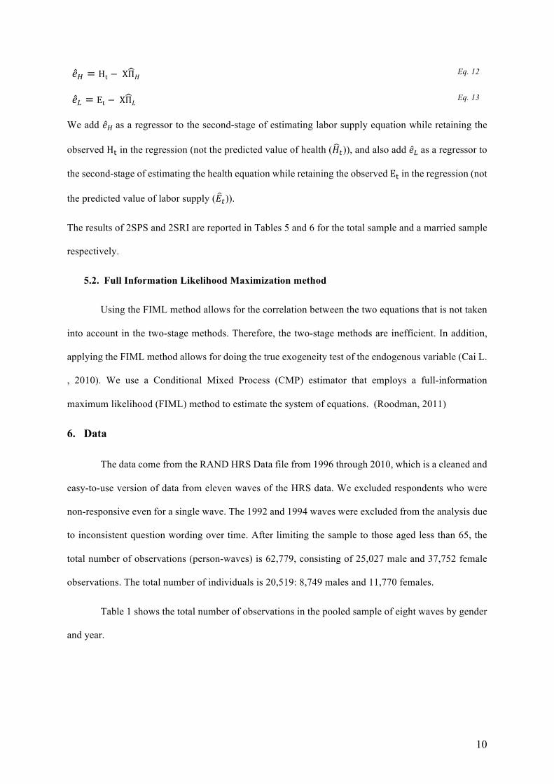
𝑒S = Ht − ΧΠ𝐻

Eq. 12

𝑒@ = Et − ΧΠ𝐿

Eq. 13

We add 𝑒S as a regressor to the second-stage of estimating labor supply equation while retaining the

observed H. in the regression (not the predicted value of health (𝐻Q)), and also add 𝑒@ as a regressor to

the second-stage of estimating the health equation while retaining the observed E. in the regression (not

the predicted value of labor supply (𝐸Q)).

The results of 2SPS and 2SRI are reported in Tables 5 and 6 for the total sample and a married sample

respectively.

5.2. Full Information Likelihood Maximization method

Using the FIML method allows for the correlation between the two equations that is not taken

into account in the two-stage methods. Therefore, the two-stage methods are inefficient. In addition,

applying the FIML method allows for doing the true exogeneity test of the endogenous variable (Cai L.

, 2010). We use a Conditional Mixed Process (CMP) estimator that employs a full-information

maximum likelihood (FIML) method to estimate the system of equations. (Roodman, 2011)

6. Data

The data come from the RAND HRS Data file from 1996 through 2010, which is a cleaned and

easy-to-use version of data from eleven waves of the HRS data. We excluded respondents who were

non-responsive even for a single wave. The 1992 and 1994 waves were excluded from the analysis due

to inconsistent question wording over time. After limiting the sample to those aged less than 65, the

total number of observations (person-waves) is 62,779, consisting of 25,027 male and 37,752 female

observations. The total number of individuals is 20,519: 8,749 males and 11,770 females.

Table 1 shows the total number of observations in the pooled sample of eight waves by gender

and year.

11

Table 1. Total Number of Observations by Gender and Year

Year Male Female No. of observations % No. of observations %

1996 3,582 14.31 5,255 13.92 1998 4,003 15.99 5,702 15.10 2000 3,263 13.04 4,844 12.83 2002 2,568 10.26 4,063 10.76 2004 3,234 12.92 4,900 12.98 2006 2,426 9.69 3,968 10.51 2008 2,022 8.08 3,291 8.72 2010 3,929 15.70 5,729 15.18 Total 25,027 100.00 37,752 100.00

Table 2 shows the total number of respondents in the pooled sample of eight waves by gender

and year.

Table 2. Total Number of Respondents by Gender and Year

Year Male Female No. of respondents % No. of respondents %

1996 3,582 40.94 5,255 44.65 1998 1,272 14.54 1,445 12.28 2000 92 1.05 150 1.27 2002 61 0.70 114 0.97 2004 1,359 15.53 1,656 14.07 2006 54 0.62 74 0.63 2008 49 0.56 48 0.41 2010 2,280 26.06 3,028 25.73 Total 8,749 100.00 11,770 100.00

7. Descriptive Statistics

Table 3 presents descriptive statistics in the pooled eight-waves sample for males and females. The

HRS is a nationally representative sample of those aged 51 and older, but spouses are included in the

data regardless of age. Our sample is restricted to males aged between 22 and 64 years old and females

aged between 23 and 64 years old. Our male sample is predominantly middle aged (mean age is

57.78), white (85 percent), married (81 percent), having health insurance (88 percent), mostly covered

by their own employers (57 percent), and are employed (70 percent), have high school diploma or more

(81.6%) . Forty-one percent live in the south. The sample of females is also predominantly middle aged

(mean age is 56.48), white (82 percent), married (70 percent), have health insurance (86 percent – 40

percent mostly covered by their own employers), are employed (58 percent), and have high school

diploma or more (80.8 percent). Forty-three percent live in the south. The summary statistics for a group

of married people are reported in the Appendix.

12

Table 3. Summary Statistics

Variable Definition Male Female Total Mean Mean Mean

Labor supply 1=working for pay, otherwise=0 0.699 0.584 0.630

Health 1=poor, 2=fair, 3=good 4=very good, 5=excellent 3.308 3.283 3.293

Northeast 1=Northeast & other, otherwise=0 0.151 0.156 0.154

Midwest 1=Midwest, otherwise=0 0.244 0.235 0.238

South 1=South, otherwise=0 0.413 0.426 0.421

West 1= West, otherwise=0 0.192 0.183 0.186

Hispanic 1= Hispanic, otherwise=0 0.114 0.117 0.115

White 1= White/ Caucasian/ Other, otherwise=0 0.850 0.819 0.831

African American 1=African American, otherwise=0 0.150 0.181 0.169

Less than high school 1=less than high school, otherwise=0 0.184 0.192 0.189

High school 1=high school, otherwise=0 0.328 0.371 0.354

College 1=college, otherwise=0 0.238 0.249 0.244

More than college 1=more than college, otherwise=0 0.250 0.188 0.213

Age Age at the middle of survey 57.78 56.48 57.00

Child 0=18 Has child (ren) under 18; 1=yes 0=no 0.120 0.0969 0.106

White collar1 White collar 1; 1=yes 0=no 0.263 0.245 0.252

White collar2 White collar 2; 1=yes 0=no 0.171 0.452 0.340

Blue collar Blue collar; 1=yes 0=no 0.407 0.117 0.232

High blood pressure Blood pressure; 1=yes 0=no 0.438 0.406 0.419

Diabetes Diabetes; 1=yes 0=no 0.157 0.133 0.142

Cancer Cancer; 1=yes 0=no 0.058 0.084 0.074

Lung Lung; 1=yes 0=no 0.053 0.065 0.061

Heart Heart attack; 1=yes 0=no 0.162 0.112 0.132

Stroke Stroke; 1=yes 0=no 0.044 0.035 0.039

Psychiatric problems Psychiatric problems; 1=yes 0=no 0.0999 0.170 0.142

Arthritis Arthritis;1=yes 0=no 0.368 0.471 0.430

Health cond. 1 No. of chronic conditions=1, otherwise=0 0.322 0.308 0.313




Health cond. 5 No. of chronic conditions=5 or more, otherwise=0 0.021 0.031 0.029

Physical functionality Single-continous index for ADL & IADL -0.456 -0.311 -0.367

Wealth Total household assets/10000 3.687 3.405 3.517

Married Married; 1=yes 0=no 0.807 0.693 0.738

Current smoker Current smoker; 1=yes 0=no 0.689 0.522 0.589

Current drinker Current heavy drinker; 1=yes 0=no 0.067 0.013 0.035

Lagged smoker Lagged smoker; 1=yes 0=no 0.449 0.360 0.395

Lagged drinker Lagged heavy drinker; 1=yes 0=no 0.042 0.009 0.022

Lagged preventive behaviors 6 Lagged preventive behavior; 1=yes 0=no 0.346 0.410 0.384

Employer-provided health insurance Employer-provided HI; 1=yes 0=no 0.571 0.399 0.467

Spousal health insurance 1=Spousal health insurance, otherwise=0 0.130 0.270 0.214

6 The preventive behavior is defined as whether the respondent reports preventive health tests and procedures such as a blood test for cholesterol, a flu shot, monthly self-checks for breast lumps, a mammogram, a pap smear, and a check for prostate cancer.

13

Health insurance Health insurance; 1=yes 0=no 0.876 0.863 0.868

Year 1996 1 if interviewed in 1996 0.143 0.139 0.141








Table 4 tabulates employment status against self-reported health status using the pooled sample.

The table shows a positive relationship between employment status and health status for both males and

females. In other words, the better the health, the more likely to be employed.

Table 4. Health against Employment Status by Gender

Employment status Health status

Poor (1)

Fair (2)

good (3)

Very good (4)

Excellent (5)

Male % non-employment 77.87 47.95 27.24 20.24 15.36 % employment 22.13 52.05 72.76 79.47 84.64

Female % non-employment 84.79 58.10 38.48 30.85 28.78 % employment 15.21 41.90 61.52 69.15 71.22

8. Endogeneity test of health

To test the endogeneity of health to the labor supply, three methods are used. We test the

endogeneity of health for the sample of males and females separately.

1). Assuming 𝜌=0, we test the significance of coefficient 𝜃S from the 2SPS method in Eq. 4. The

result of test indicates that health is endogenous to the labor supply for both males and females. This

method assumes that the correlation between two equations is zero, and this is the disadvantage of this

method (Stern, 1989). The results are reported in the Appendix.

2). We use an augmented Hausman test that was first proposed by (Hausman, 1978), and then

developed by Smith and Blundell (1986). We use 2SRI results and add the first-stage residuals to the

second-stage of the labor supply regression as an exogenous regressor. If the coefficient of the added

regressor is significant, then exogeneity is rejected. The result for the sample of males indicates that

health is endogenous with respect to labor supply for both males and females. Both methods assume

14

that the correlation between two equations are zero (𝜌=0). Therefore, they are only partial tests for

endogeneity of health.

3). To conduct a true test of exogeneity, we follow (Cai L. , 2010), and use the FIML estimation

results to measure the joint significant of 𝜃S and 𝜌. We test the following hypothesis.

H0 ∶ 𝜃S = 0, 𝛿�@ � = 0, and 𝛿�@ � = 0 H1 ∶ 𝜃S ≠ 0, 𝛿�@(�) ≠ 0, and 𝛿�@(�) ≠ 0

where 𝜃S, 𝛿�@(�) and 𝛿�@(�) are the coefficient on the labor supply variable, the covariance of the time-

invariant error component, and the correlation coefficient of time-variant error components

respectively. The test statistic is significant for both males and females, implying that health should not

be treated as exogenous to labor supply. All results are reported in the Appendix.

9. Results

Table 5 provides the results of two-stage models of 2SPS and 2SRI, and FIML for males and

females.

Table 5. Estimates of coefficients of labor supply and health equations

Male Female 2SPS 2SRI FIML 2SPS 2SRI FIML

Labor Supply equation

Health 0.8776*** 0.9814*** 0.5822*** 0.6308*** 0.7459*** 0.4615*** (0.041) (0.042) (0.019) (0.025) (0.028) (0.023) 1st stage residual of LS eq. -0.7145*** -0.5530*** (0.041) (0.028) Age 0.2991*** 0.3131*** 0.3578*** 0.4618*** 0.4653*** 0.4169*** (0.086) (0.087) (0.083) (0.053) (0.052) (0.051) Age squared -0.0037*** -0.0039*** -0.0043*** -0.0052*** -0.0052*** -0.0048*** (0.001) (0.001) (0.001) (0.000) (0.000) (0.000) Married 0.3094*** 0.3139*** 0.2442*** -0.3672*** -0.3762*** -0.3098*** (0.074) (0.074) (0.070) (0.052) (0.052) (0.053) Child 0-18 0.2408 0.2362 0.3499 0.1297 0.1245 0.0790 (0.207) (0.210) (0.221) (0.141) (0.142) (0.184) Married*Child 0-18 -0.1476 -0.1442 -0.2378 -0.3574** -0.3542** -0.2938 (0.224) (0.227) (0.236) (0.158) (0.159) (0.203) Less than high school 0.2375** 0.2331** 0.0885 -0.1981** -0.1752** -0.2745*** (0.105) (0.104) (0.090) (0.078) (0.078) (0.078) Age 62+ -0.5709*** -0.5700*** -0.2944*** -0.1898*** -0.1912*** -0.1755** (0.094) (0.094) (0.087) (0.068) (0.067) (0.088) Less than high school*Age 62+

0.0808 0.0877 0.1215 0.2361** 0.2312** 0.2046

(0.128) (0.127) (0.132) (0.104) (0.105) (0.141) College -0.0558 -0.0585 0.0432 0.2341*** 0.2253*** 0.2338*** (0.093) (0.093) (0.082) (0.067) (0.067) (0.066) College*Age 62+ 0.2233* 0.2341* 0.1287 0.0041 0.0007 0.0337 (0.126) (0.126) (0.130) (0.095) (0.095) (0.133) More than College 0.0026 0.0078 0.1773* 0.2328*** 0.2061** 0.2957*** (0.107) (0.107) (0.093) (0.084) (0.083) (0.080) More than college*Age 62+ 0.2170* 0.2236* 0.1789 0.0470 0.0453 0.0310 (0.121) (0.121) (0.127) (0.107) (0.106) (0.149) White collar 2 0.2321** 0.2283** 0.1895** 0.6322*** 0.6290*** 0.5894***

15

(0.091) (0.090) (0.078) (0.057) (0.057) (0.053) Blue collar 0.0224 0.0210 -0.0104 0.6928*** 0.6935*** 0.6121*** (0.078) (0.078) (0.068) (0.084) (0.083) (0.078) Wealth -0.0021 -0.0026 0.0003 -0.0084** -0.0086** -0.0087*** (0.002) (0.002) (0.003) (0.004) (0.004) (0.002) Hispanic 0.3987*** 0.4055*** 0.3473*** 0.2881*** 0.3116*** 0.1869** (0.113) (0.112) (0.097) (0.084) (0.084) (0.083) African American -0.0544 -0.0541 -0.0410 0.2068*** 0.2269*** 0.1318** (0.091) (0.090) (0.079) (0.068) (0.067) (0.065) Midwest 0.0332 0.0237 0.0523 0.1442** 0.1409** 0.1536*** (0.077) (0.077) (0.067) (0.060) (0.060) (0.057) Northeast -0.0130 -0.0150 -0.0163 0.1949*** 0.1923*** 0.1969*** (0.093) (0.092) (0.080) (0.071) (0.071) (0.066) West 0.0896 0.0872 0.0254 -0.0884 -0.0939 -0.0437 (0.087) (0.086) (0.076) (0.068) (0.068) (0.064) Employer_provided HI 0.7913*** 0.7937*** 0.6765*** 1.5247*** 1.5218*** 1.3867*** (0.058) (0.058) (0.049) (0.047) (0.047) (0.052) Year 1996 -0.3921*** -0.3838*** 0.0206 -0.5443*** -0.5596*** -0.3631*** (0.086) (0.086) (0.089) (0.063) (0.063) (0.088) Year 1998 -0.1468* -0.1302 -0.1548* -0.2688*** -0.2747*** -0.3299*** (0.082) (0.081) (0.085) (0.059) (0.059) (0.086) Year 2000 -0.2809*** -0.2710*** -0.0254 -0.4395*** -0.4487*** -0.3084*** (0.082) (0.081) (0.090) (0.059) (0.059) (0.091) Year 2002 -0.4439*** -0.4431*** -0.1328 -0.4288*** -0.4360*** -0.3277*** (0.082) (0.082) (0.096) (0.056) (0.056) (0.094) Year 2004 -0.1635** -0.1565** -0.0819 -0.2863*** -0.2901*** -0.2709*** (0.074) (0.074) (0.087) (0.050) (0.051) (0.087) Year 2006 -0.0803 -0.0731 0.0769 -0.2408*** -0.2422*** -0.0854 (0.068) (0.068) (0.095) (0.047) (0.047) (0.094) Constant -1.8920 -3.5139 -3.5100* -8.0951*** -8.8633*** -7.2926*** (2.355) (2.366) (2.010) (1.390) (1.383) (1.396)

Health equation

Labor supply 0.1846*** 0.4576*** 0.4615*** 0.0215 0.2342*** 0.0106 (0.026) (0.038) (0.023) (0.014) (0.025) (0.012) Age -0.1631*** -0.1697*** -0.1705*** -0.0606** -0.0596** -0.0721** (0.037) (0.037) (0.045) (0.028) (0.028) (0.036) Age squared 0.0018*** 0.0018*** 0.0019*** 0.0007*** 0.0007*** 0.0008** (0.000) (0.000) (0.000) (0.000) (0.000) (0.000) White collar 2 -0.1276*** -0.1261*** -0.1412*** 0.0224 0.0229 0.0215 (0.046) (0.046) (0.047) (0.034) (0.034) (0.034) Blue collar -0.1604*** -0.1609*** -0.1448*** -0.1539*** -0.1539*** -0.1569*** (0.042) (0.042) (0.042) (0.048) (0.048) (0.050) Wealth 0.0027** 0.0028** 0.0024* 0.0031*** 0.0031** 0.0034** (0.001) (0.001) (0.001) (0.001) (0.001) (0.001) Hispanic -0.4477*** -0.4477*** -0.4763*** -0.6691*** -0.6718*** -0.6672*** (0.064) (0.064) (0.059) (0.056) (0.055) (0.053) African American -0.1545*** -0.1553*** -0.1935*** -0.3981*** -0.3992*** -0.3925*** (0.051) (0.051) (0.049) (0.040) (0.040) (0.042) Midwest 0.0479 0.0484 0.0424 0.1018*** 0.1024*** 0.1143*** (0.041) (0.040) (0.041) (0.036) (0.036) (0.037) Northeast 0.0761 0.0764 0.0847* 0.0581 0.0591 0.0657 (0.049) (0.049) (0.048) (0.043) (0.043) (0.043) West -0.0018 -0.0007 0.0212 0.0808* 0.0820* 0.0657 (0.048) (0.048) (0.046) (0.043) (0.042) (0.041) Physical functionality -0.1782*** -0.1829*** -0.2253*** -0.2431*** -0.2471*** -0.2573*** (0.019) (0.019) (0.012) (0.012) (0.012) (0.010) No. of chronic conditions -0.3805*** -0.3821*** -0.3539*** -0.5163*** -0.5179*** -0.5129*** (0.032) (0.032) (0.029) (0.027) (0.026) (0.030) Married -0.0332 -0.0320 -0.0428 0.1337*** 0.1334*** 0.1358*** (0.042) (0.041) (0.043) (0.031) (0.031) (0.033) Less than high school -0.3697*** -0.3675*** -0.3648*** -0.4930*** -0.4919*** -0.4962*** (0.051) (0.051) (0.049) (0.046) (0.046) (0.043) College 0.1949*** 0.1946*** 0.1805*** 0.2463*** 0.2480*** 0.2592*** (0.046) (0.045) (0.044) (0.039) (0.039) (0.038) More than college 0.4255*** 0.4304*** 0.3973*** 0.5932*** 0.5933*** 0.6128*** (0.052) (0.052) (0.050) (0.048) (0.048) (0.046) Current smoker -0.0951** -0.0989** -0.1336*** -0.0540 -0.0541 -0.0653 (0.043) (0.042) (0.040) (0.036) (0.035) (0.042) Current heavy drinker -0.0973* -0.0969* -0.0662 -0.2228** -0.2255** -0.2146 (0.053) (0.052) (0.060) (0.096) (0.096) (0.142) Lagged smoker -0.0800*** -0.0788*** -0.0558 -0.0381 -0.0380 -0.0393 (0.030) (0.030) (0.041) (0.027) (0.027) (0.046) Lagged heavy drinker -0.0722 -0.0721 -0.0401 0.1197 0.1200 0.0480

16

(0.054) (0.054) (0.073) (0.098) (0.098) (0.162) Lagged preventive behavior 0.0074 0.0077 -0.0065 -0.0512*** -0.0514*** -0.0462 (0.020) (0.020) (0.034) (0.015) (0.015) (0.031) High blood pressure -0.0157 -0.0150 0.0245 0.0087 0.0102 0.0310 (0.044) (0.044) (0.041) (0.039) (0.039) (0.045) Diabetes -0.2182*** -0.2209*** -0.1762*** -0.1912*** -0.1933*** -0.1753*** (0.053) (0.053) (0.048) (0.048) (0.048) (0.054) Cancer -0.2708*** -0.2731*** -0.2642*** -0.0586 -0.0553 -0.0490 (0.080) (0.079) (0.063) (0.058) (0.057) (0.058) Lung diseases -0.4046*** -0.4065*** -0.3412*** -0.2581*** -0.2613*** -0.2511*** (0.079) (0.078) (0.069) (0.067) (0.067) (0.068) Heart -0.2699*** -0.2693*** -0.2989*** -0.1662*** -0.1668*** -0.1697*** (0.053) (0.053) (0.047) (0.053) (0.052) (0.057) Stroke 0.0770 0.0782 -0.0564 0.2331*** 0.2311*** 0.2126** (0.085) (0.083) (0.074) (0.089) (0.089) (0.089) Psychiatric problem -0.0541 -0.0567 -0.1510*** -0.0636 -0.0657 -0.0931* (0.068) (0.067) (0.058) (0.049) (0.049) (0.053) Health insurance 0.1334*** 0.1398*** 0.0473 0.1532*** 0.1520*** 0.1127** (0.044) (0.044) (0.048) (0.034) (0.034) (0.047) 1st stage residual of H eq. -0.1304*** 0.0222 (0.027) (0.015) Cut_1 -6.6684*** -6.7227*** -6.7620*** -4.8849*** -4.7380*** 0.0106 (0.981) (0.976) (1.329) (0.750) (0.745) (0.012) Cut_2 -5.1833*** -5.2285*** -5.2533*** -3.1948*** -3.0407*** -5.2387*** (0.981) (0.976) (1.328) (0.749) (0.743) (0.983) Cut_3 -3.6254*** -3.6692*** -3.6970*** -1.5797** -1.4229* -3.5415*** (0.981) (0.976) (0.748) (0.743) (0.982) Cut_4 -2.0079** -2.0542** -2.0927 0.1976 0.3538 -1.9281** (0.981) (0.976) (1.328) (0.748) (0.743) (0.981)

Log-likelihood of LS eq. -6890 -6830 -29449 -11501 -11428 -44844 Log-likelihood of H eq. -20164 -20102 -29449 -30500 -30440 -44844 Ln(𝛿@(�)) 1.1323*** 1.1060*** 0.9805*** 0.9638*** (0.066) (0.067) (0.047) (0.047) 𝛿�(�) 1.0526*** 1.0234*** 1.2668*** 1.2503*** (0.045) (0.044) (0.042) (0.041) 𝛿�@(�) -0.5416*** -0.5416*** -0.1361*** (0.038) (0.038) (0.038) 𝛿@�(�) -0.8222*** -0.8222*** -0.4076*** (0.029) (0.029) (0.030) Number of individuals 6,022 8,323 Observations 17,271 27,468

Robust standard errors in parentheses *** p<0.01, ** p<0.05, * p<0.1

Table 6 represents the results of two-stage models of 2SPS and 2SRI, and FIML for a group of

married males and females. To address the endogeneity of employer-provided health insurance to

labor supply, we rerun the models for a married sample.

Table 6. Estimates of coefficients of labor supply and health for a group of married males and females

Male Female 2SPS 2SRI FIML 2SPS 2SRI FIML

Labor supply equation

Health 0.3166*** 0.9980*** 0.6692*** 0.6714*** 0.7540*** 0.5375*** (0.115) (0.046) (0.017) (0.034) (0.035) (0.025) 1st stage residual -0.7025*** -0.5694*** (0.045) (0.036) Age 0.3166*** 0.3230*** 0.4593*** 0.5168*** 0.5148*** 0.5468*** (0.115) (0.115) (0.055) (0.068) (0.067) (0.064) Age squared -0.0040*** -0.0041*** -0.0052*** -0.0059*** -0.0059*** -0.0061*** (0.001) (0.001) (0.000) (0.001) (0.001) (0.001) Child 0-18 0.0250 0.0277 0.0504 -0.3499*** -0.3511*** -0.2970*** (0.101) (0.101) (0.063) (0.090) (0.090) (0.106) Less than high school 0.1529 0.1479 -0.0069 -0.3756*** -0.3778*** -0.3624*** (0.124) (0.121) (0.094) (0.106) (0.105) (0.099)

17

Age 62+ -0.4958*** -0.4966*** -0.1383* -0.2735*** -0.2785*** -0.1392 (0.000) (0.106) (0.072) (0.083) (0.083) (0.109) Less than high school*Age 62+ -0.0486 -0.0391 0.0751 0.2318* 0.2314* 0.2436 (0.148) (0.147) (0.111) (0.137) (0.138) (0.188) College -0.0171 -0.0174 0.0667 0.3488*** 0.3481*** 0.2781*** (0.109) (0.108) (0.085) (0.085) (0.085) (0.080) College*Age 62+ 0.2140 0.2222 0.0770 0.0555 0.0578 0.0837 (0.143) (0.143) (0.109) (0.117) (0.117) (0.166) More than college 0.0182 0.0251 0.1421 0.4437*** 0.4461*** 0.4012*** (0.122) (0.120) (0.094) (0.105) (0.105) (0.096) More than college*Age 62+ 0.1726 0.1797 0.0819 0.0465 0.0448 0.0284 (0.134) (0.133) (0.104) (0.127) (0.126) (0.184) White collar 2 0.1419 0.1389 0.1193 0.7295*** 0.7306*** 0.6228*** (0.102) (0.101) (0.083) (0.075) (0.075) (0.064) Blue collar -0.1039 -0.1013 -0.1058 0.8017*** 0.8022*** 0.7210*** (0.090) (0.088) (0.073) (0.110) (0.110) (0.098) Wealth -0.0027 -0.0030* -0.0018 -0.0076** -0.0077** -0.0071*** (0.002) (0.002) (0.003) (0.003) (0.003) (0.002) Hispanic 0.3701*** 0.3761*** 0.3397*** 0.1403 0.1434 0.0816 (0.129) (0.128) (0.103) (0.113) (0.113) (0.104) African African -0.0157 -0.0163 0.0268 0.5665*** 0.5681*** 0.4374*** (0.112) (0.110) (0.089) (0.098) (0.097) (0.089) Midwest 0.0295 0.0165 0.0413 0.2753*** 0.2777*** 0.2522*** (0.087) (0.086) (0.071) (0.076) (0.075) (0.070) Northeast 0.0471 0.0460 0.0449 0.4157*** 0.4184*** 0.3493*** (0.106) (0.105) (0.084) (0.093) (0.093) (0.083) west 0.0481 0.0465 0.0210 -0.1670* -0.1668* -0.1617** (0.100) (0.098) (0.080) (0.089) (0.088) (0.078) Spousal health insurance -0.4838*** 0.3230*** -0.3203*** -0.8283*** -0.8310*** -0.7097*** (0.076) (0.115) (0.050) (0.048) (0.048) (0.058) Year 1996 -0.3397*** -0.0041*** 0.0079 -0.6591*** -0.6585*** -0.4944*** (0.098) (0.001) (0.076) (0.080) (0.079) (0.114) Year 1998 -0.1162 0.0277 -0.1198 -0.4426*** -0.4450*** -0.4280*** (0.093) (0.101) (0.074) (0.074) (0.074) (0.107) Year 2000 -0.2234** 0.1479 -0.0153 -0.5280*** -0.5276*** -0.4063*** (0.092) (0.121) (0.075) (0.074) (0.073) (0.119) Year 2002 -0.3498*** -0.4966*** -0.0836 -0.4766*** -0.4772*** -0.3762*** (0.092) (0.106) (0.082) (0.069) (0.069) (0.121) Year 2004 -0.0929 -0.0391 -0.0485 -0.3416*** -0.3423*** -0.2709** (0.085) (0.147) (0.073) (0.062) (0.062) (0.109) Year 2006 -0.0720 -0.0174 0.0380 -0.2634*** -0.2614*** -0.1437 (0.076) (0.108) (0.082) (0.056) (0.056) (0.200) Constant 0.0266 -1.7523 -4.2115*** -8.6199*** -9.3649*** -10.1590** (3.186) (3.188) (1.551)) (1.784) (1.782) (1.713)

Health equation

Labor supply 0.1120*** 0.4039*** 0.3998*** -0.0174 0.1678*** -0.0246 (0.050) (0.058) (0.014) (0.026) (0.036) (0.024) Age -0.1449*** -0.1576*** -0.2567*** -0.0266 -0.0271 -0.0407 (0.048) (0.047) (0.006) (0.035) (0.035) (0.035) Age squared 0.0015*** 0.0016*** 0.0028*** 0.0003 0.0003 0.0004 (0.000) (0.000) (0.000) (0.000) (0.000) (0.000) White collar 2 -0.1109** -0.1093** -0.1273** 0.0301 0.0303 0.0194 (0.052) (0.051) (0.056) (0.043) (0.043) (0.043) Blue collar -0.1575*** -0.1582*** -0.0741 -0.1563*** -0.1555*** -0.1879*** (0.049) (0.048) (0.050) (0.060) (0.060) (0.064) Wealth 0.0033*** 0.0033*** 0.0030* 0.0026** 0.0026** 0.0027* (0.001) (0.001) (0.002) (0.001) (0.001) (0.002) Hispanic -0.4664*** -0.4655*** -0.4866*** -0.7014*** -0.7039*** -0.6806*** (0.073) (0.072) (0.071) (0.069) (0.068) (0.066) African American -0.1600*** -0.1605*** -0.1688*** -0.4193*** -0.4198*** -0.4103*** (0.060) (0.059) (0.062) (0.054) (0.054) (0.057) Midwest 0.0807* 0.0816* 0.0450 0.1410*** 0.1420*** 0.1574*** (0.045) (0.045) (0.049) (0.043) (0.043) (0.044) Northeast 0.1010* 0.1017* 0.0592 0.1257** 0.1280** 0.1252** (0.055) (0.055) (0.058) (0.054) (0.054) (0.053) West -0.0061 -0.0065 -0.0076 0.0962* 0.0972* 0.0975** (0.054) (0.053) (0.055) (0.052) (0.051) (0.050) Physical functionality -0.2255*** -0.2292*** -0.2056*** -0.2861*** -0.2892*** -0.2980*** (0.029) (0.028) (0.012) (0.019) (0.019) (0.014) No. of chronic conditions -0.4280*** -0.4295*** -0.3068*** -0.5224*** -0.5238*** -0.5061*** (0.038) (0.037) (0.027) (0.032) (0.032) (0.036) Less than high school -0.3611*** -0.3585*** -0.2666*** -0.5614*** -0.5615*** -0.5397*** (0.059) (0.058) (0.059) (0.058) (0.058) (0.056)

18

College 0.2283*** 0.2271*** 0.1468*** 0.2570*** 0.2588*** 0.2495*** (0.054) (0.053) (0.054) (0.048) (0.048) (0.046) More than college 0.4561*** 0.4605*** 0.2886*** 0.6147*** 0.6160*** 0.6298*** (0.063) (0.062) (0.059) (0.060) (0.060) (0.056) Current smoker -0.1200** -0.1235** -0.1303*** -0.0223 -0.0226 -0.0320 (0.048) (0.048) (0.038) (0.043) (0.043) (0.051) Current heavy drinker -0.1066* -0.1065* -0.0536 -0.0666 -0.0691 -0.0566 (0.061) (0.061) (0.061) (0.121) (0.121) (0.198) Lagged smoker -0.0812** -0.0807** -0.0475 -0.0458 -0.0455 -0.0405 (0.034) (0.034) (0.040) (0.033) (0.033) (0.056) Lagged heavy drinker -0.0715 -0.0708 -0.0364 0.2726** 0.2696** 0.1984 (0.064) (0.064) (0.074) (0.133) (0.132) (0.225) Lagged preventive behavior 0.0022 0.0028 -0.0054 -0.0380** -0.0383** -0.0330 (0.023) (0.023) (0.034) (0.018) (0.018) (0.038) High blood pressure 0.0378 0.0378 0.0399 0.0018 0.0022 0.0232 (0.050) (0.049) (0.038) (0.047) (0.047) (0.053) Diabetes -0.2209*** -0.2246*** -0.1524*** -0.2566*** -0.2588*** -0.2397*** (0.059) (0.059) (0.045) (0.058) (0.058) (0.066) Cancer -0.3726*** -0.3711*** -0.2513*** -0.0408 -0.0373 -0.0389 (0.088) (0.087) (0.059) (0.071) (0.070) (0.070) Lung diseases -0.4501*** -0.4481*** -0.3483*** -0.2303*** -0.2307*** -0.2420*** (0.090) (0.089) (0.067) (0.086) (0.086) (0.087) Heart -0.2728*** -0.2713*** -0.2390*** -0.2244*** -0.2233*** -0.2058*** (0.061) (0.061) (0.044) (0.065) (0.065) (0.070) Stroke -0.0072 0.0009 -0.1095 0.2663** 0.2662** 0.2186* (0.102) (0.099) (0.072) (0.118) (0.118) (0.114) Psychiatric problems -0.0983 -0.1029 -0.1438** -0.0732 -0.0733 -0.0946 (0.079) (0.078) (0.056) (0.059) (0.059) (0.065) Health insurance 0.2131*** 0.2196*** 0.2156*** 0.1810*** 0.1794*** 0.2549*** (0.056) (0.056) (0.047) (0.045) (0.045) (0.060) 1st stage residual of H eq. -0.0577 0.0541** (0.051) (0.026) Cut_1 -6.5853*** -6.8018*** -8.4287 -4.2938*** -4.2010*** -4.5986*** (1.224) (1.207) (0.000) (0.920) (0.918) (0.945) Cut_2 -5.0639*** -5.2693*** -6.9179*** -2.5873*** -2.4875*** -2.8996*** (1.224) (1.207) (0.032) (0.920) (0.918) (0.943) Cut_3 -3.4538*** -3.6589*** -5.3312*** -0.9142 -0.8105 -1.2265 (1.224) (1.207) (0.042) (0.920) (0.917) (0.942) Cut_4 -1.7828** -1.9823** -3.6926*** 0.9461 1.0500 0.6179 (1.224) (0.207) (0.055) (0.920) (0.917) (0.941)

Log-likelihood of LS eq. -6890 -6830 -29449 -11501 -11428 -44844 Log-likelihood of H eq. -16240 -16185 -21497 -21464 -44844 Ln(𝛿@(�)) 1.2332*** 1.1863*** 1.2573*** 1.2478*** (0.075) (0.075) (0.055) (0.055) 𝛿�(�) 1.1156*** 1.0767*** 1.3402*** 1.3323*** (0.052) (0.051) (0.053) (0.052) 𝛿�@(�) -0.9145*** -0.2039*** (0.040) (0.056) 𝛿@�(�) -1.1420*** -0.4895*** (0.030) (0.040) Total Log-likelihood -23879 -32064 Number of individuals 5,076 6,144 Observations 14,081 19,690

Robust standard errors in parentheses *** p<0.01, ** p<0.05, * p<0.1

Focusing on the results from 2SPS and 2SRI methods in the labor supply equation for the married

sample, as we expected, there is a positive significant relationship between health status and labor

supply for both males and females. The better is health, the more likely one is to work. We find that

the effect of age on the labor supply is significant and negative for those older than 62 years for both

males and females. The presence of children younger than 18 has a positive and strongly significant

affect on women’s supply of labor. However, this effect is not significant for males. More education

19

is associated with higher labor supply for females. The effect of education is not statistically

significant determinant of labor supply for males. Compared to white collar 1 women workers, white

collar 2 and blue collar women workers are more likely to be employed. However, the effect is

insignificant for males. Hispanic men are more likely to work, and the result is insignificant for

women. Compared to Whites, African-American women are more likely to be employed, and there is

no significant association between race and labor supply for males. Women who live in Midwestern

and Northeastern states are more likely to be employed than women who live in the South. The effect

of health insurance is strongly significant for both males and females. Those with spousal health

insurance are less likely to be employed. In 1996 and 2002, we have a lower probability of working

compared to 2010.7

Focusing on the results from the 2SPS and 2SRI methods in the health equation for the married

sample (Table 6), we find a significant positive association between labor supply and health for

males. For females, the result of the 2SRI method is positive and significant. However, the same

result from the 2SPS method is negative and insignificant. As we expected, age has a significant

negative effect and a insignificant positive effect for males and females respectively. The positive

sign of age squared implies that the age effect becomes stronger as people age. White collar 2 and

blue collar men workers are likely to have a better health status than white collar 1 men workers. The

same results for blue collar women workers. Both Hispanics and African-Americans have poorer

health outcomes compared with non-Hispanic whites. The census region is statistically significant for

females but not for males. The poorer physical functionality and the higher number of chronic

illnesses suggest poorer health outcomes for both males and females. Education has a strong direct

effect on health. Among males, current/lagged smokers and current heavy drinkers have poorer health

outcomes compared with non-smokers/drinkers. Smoking and drinking have no significant effects on

females’ health. Lagged preventive behaviors have a negative significant effect on health. Most

chronic illnesses have a positive significant effect on health for both males and females. Those with

health insurance are more likely to have better health status.

7 2010 is the omitted benchmark year, but 2008 is also omitted because of collinearity

20

Focusing on the results of FIML estimation, the effect of health on the labor supply is

statistically significant and positive. The reverse effect of the labor supply on health is

positive and significant for males, but negative and insignificant for females. The reverse

effect for males do not support the result was found in (Cai L. , 2010). The estimated time-

varying unobserved error terms (𝛿�@(�) and 𝛿@�(�)) are both negative and statistically

significant. For males, the positive effect of labor supply on health would lead an upward bias

in the estimate of the effect of health on the labor supply. Meanwhile, the negative correlation

between the health and labor supply equations implies a downward bias in the estimate of the

effect of health on labor supply. Overall, the ambiguous net effect suggesting that it is not

possible to measure the direction of the bias caused by the endogeneity of health for males.

For females, although the effect of labor supply on health is negative, it is insignificant.

10. Conclusion

Using partial information maximum likelihood (PIML) methods (2SPS and 2SRI) and full

information maximum likelihood (FIML), we estimated the relationship between health and labor

supply equations. We used three methods to check the possible endogeneity of health with respect to

labor supply. The results of the endogeneity tests confirmed the results of previous studies (Stern, 1989;

Cai L. , 2010) that health should not be treated as exogenous. To address the endogeneity of health, a

simultaneous equations model was used. Using RAND longitudinal HRS data 1996-2010, we found a

positive significant effect of health on labor supply for both males and females using three estimation

methods. However, the reverse effect of labor supply on health does not support the finding in (Cai L.

, 2010). We found a significant positive effect of labor supply on health for males using all methods,

and positive and significant effect of labor supply on health in the 2SRI method for females. For males,

the source of endogeneity of health is not clear because of negative correlation between health and labor

supply, and positive effect of labor on health.

21

We found evidence for the significant role of health insurance in the decision to work among

married women and men. Those insured through their spouses’ health insurance tend to work less than

those without spousal health insurance.

The results also confirmed the finding in (Cai L. , 2010) that there were efficiency gains in

using panel data. The evidence indicated that the variances of the time-varying unobserved error terms

are large and highly significant in both equations.

22

APPENDIX Table 7. Summary statistics of married males and females

Variables Male Female Total Mean Mean Mean

Labor supply 0.724 0.585 0.646

Health 3.361 3.410 3.388

Northeast 0.151 0.149 0.150

Midwest 0.250 0.244 0.247

South 0.408 0.419 0.414

West 0.190 0.187 0.189

Hispanic 0.113 0.113 0.113

White 0.879 0.878 0.879

African American 0.121 0.122 0.121

Less than high school 0.175 0.165 0.169

High school 0.322 0.379 0.354

College 0.233 0.250 0.243

More than college 0.269 0.206 0.233

Age 57.91 56.11 56.89

Child 0-18 0.131 0.109 0.119

White collar1 0.286 0.266 0.274

White collar2 0.170 0.450 0.328

Blue collar 0.404 0.112 0.239

High blood pressure 0.427 0.375 0.398

Diabetes 0.156 0.119 0.135

Cancer 0.058 0.082 0.072

Lung 0.048 0.051 0.050

Heart 0.162 0.0967 0.125

Stroke 0.038 0.028 0.032

Psychiatric 0.085 0.146 0.120

Arthritis 0.364 0.447 0.411

Health cond. 1 0.328 0.323 0.325

Health cond. 2 0.211 0.214 0.213

Health cond. 3 0.105 0.104 0.104

Health cond. 4 0.040 0.044 0.042

Health cond. 5 0.021 0.020 0.021

Wealth/10000 4.104 4.262 4.193

Current smoker 0.673 0.482 0.565

Current drinker 0.057 0.009 0.030

Lagged smoker 0.445 0.338 0.384

Lagged drinker 0.036 0.006 0.019

23

Lagged preventive 0.357 0.416 0.390

Employer-provided health insurance 0.597 0.376 0.472

Spousal health insurance 0.158 0.367 0.276

Health insurance 0.901 0.886 0.893

Year 1996 0.149 0.145 0.147

Year 1998 0.164 0.157 0.160

Year 2000 0.133 0.133 0.133

Year 2002 0.105 0.110 0.108

Year 2004 0.130 0.129 0.130

Year 2006 0.097 0.105 0.102

Year 2008 0.078 0.086 0.083

Year 2010 0.143 0.135 0.138

Table 8. Alternative model

Male Female 2SPS 2SRI 2SPS 2SRI

Labor Supply equation Health 0.7782*** 1.0907*** 0.3210*** 0.5513*** (0.130) (0.132) (0.124) (0.125) 1st stage health residuals N/A -0.6166*** N/A -0.2084* N/A (0.130) N/A (0.124) Physical functioning -0.3298*** -0.3285*** -0.3861*** -0.3780*** (0.078) (0.076) (0.069) (0.068) Health condition 18 0.3419* 0.3270 0.0976 0.0767 (0.207) (0.205) (0.195) (0.194) Health condition 2 0.6109* 0.6078* 0.0096 -0.0197 (0.337) (0.334) (0.329) (0.326) Health condition 3 0.0201 0.0132 -0.2293 -0.2241 (0.184) (0.183) (0.164) (0.163) Health condition 4 -0.5795* -0.5779* -0.8077*** -0.8122*** (0.339) (0.336) (0.282) (0.278) Health condition 5 0.0713 0.0898 -0.8302** -0.8138** (0.405) (0.391) (0.330) (0.324) Age 0.5439*** 0.5652*** 0.8109*** 0.8090*** (0.158) (0.159) (0.094) (0.094) Age squared -0.0069*** -0.0071*** -0.0092*** -0.0092*** (0.001) (0.001) (0.001) (0.001) Married 0.5121*** 0.5206*** -0.5998*** -0.5978*** (0.132) (0.131) (0.101) (0.101) Child 0-18 0.3822 0.3782 0.1760 0.1777 (0.367) (0.373) (0.250) (0.249) Married*Child 0-18 -0.1696 -0.1758 -0.5814** -0.5812** (0.398) (0.404) (0.282) (0.281) Less than high school 0.4656** 0.4476** -0.5861*** -0.5995*** (0.213) (0.211) (0.187) (0.185) Age 62+ -0.9770*** -0.9814*** -0.3236*** -0.3250*** (0.167) (0.168) (0.121) (0.120) Less than high school*Age 62+ 0.1178 0.1391 0.4211** 0.4290** (0.227) (0.226) (0.188) (0.188) College -0.0599 -0.0627 0.5633*** 0.5663*** (0.174) (0.173) (0.131) (0.130) College*Age 62+ 0.3789* 0.3972* 0.0006 -0.0020 (0.224) (0.225) (0.170) (0.169) More than college 0.0925 0.1048 0.7772*** 0.7913*** (0.226) (0.225) (0.201) (0.200) More than college*Age 62+ 0.3888* 0.4008* -0.0026 -0.0115 (0.215) (0.216) (0.190) (0.189) White collar 2 0.3777** 0.3707** 1.1373*** 1.1365*** (0.163) (0.163) (0.102) (0.102) Blue collar 0.0016 -0.0018 1.1490*** 1.1429*** (0.147) (0.146) (0.153) (0.152) Wealth -0.0032 -0.0040 -0.0148 -0.0152

8 Health condition 1, Health condition 2, Health condition 3, Health condition 4, Health condition 5 are having one chronic illness, two chronic illnesses, three chronic illnesses, four chronic illnesses, and five or more than five chronic illnesses.

24

(0.003) (0.003) (0.009) (0.010) Hispanic 0.7560*** 0.7669*** 0.2079 0.2063 (0.225) (0.225) (0.212) (0.211) African American -0.1150 -0.1222 0.1650 0.1635 (0.165) (0.163) (0.145) (0.144) Mid West 0.0845 0.0682 0.3273*** 0.3288*** (0.137) (0.136) (0.108) (0.108) North East -0.0328 -0.0366 0.3703*** 0.3745*** (0.164) (0.163) (0.127) (0.126) West 0.1850 0.1825 -0.1033 -0.1060 (0.154) (0.153) (0.121) (0.121) Employer-provided health insurance 1.4290*** 1.4308*** 2.7717*** 2.7779*** (0.117) (0.116) (0.087) (0.088) Year 1996 -0.5538*** -0.5377*** -0.7708*** -0.7670*** (0.159) (0.159) (0.121) (0.121) Year 1998 -0.1574 -0.1273 -0.4592*** -0.4615*** (0.146) (0.146) (0.111) (0.111) Year 2000 -0.3957*** -0.3786*** -0.6564*** -0.6506*** (0.146) (0.146) (0.109) (0.109) Year 2002 -0.7326*** -0.7246*** -0.7058*** -0.7011*** (0.147) (0.147) (0.102) (0.102) Year 2004 -0.2347* -0.2176* -0.4630*** -0.4605*** (0.131) (0.131) (0.091) (0.091) Year 2006 -0.1443 -0.1282 -0.3605*** -0.3526*** (0.121) (0.122) (0.087) (0.087) Constant -4.2356 -6.9912 -15.3450*** -16.8186*** (4.321) (4.340) (2.454) (2.455)

Table 8. Endogeneity test of health Methods Hypothesis Male Female

(1) H0: 𝜃S = 0

H1: 𝜃S ≠ 0

t-statistics=110.8736 d.f.=17270 pr (|T|>|t|)=0.0000

t-statistics=59.9103 d.f.=27467 pr (|T|>|t|)=0.0000

(2) H0: 1𝑠𝑡 − 𝑠𝑡𝑎𝑔𝑒 𝑟𝑒𝑑𝑖𝑑𝑢𝑎𝑙𝑠 = 0

H1: 1𝑠𝑡 − 𝑠𝑡𝑎𝑔𝑒 𝑟𝑒𝑑𝑖𝑑𝑢𝑎𝑙𝑠 ≠ 0

t-statistics=755.3238 d.f.=17,270 pr (|T|>|t|)=0.0000

t-statistics=825.6941 d.f.=27,467 pr (|T|>|t|)=0.0000

(3) H0 ∶ θB = 0, δ�1 � = 0, and δ�1 � = 0 H1 ∶ θB ≠ 0, δ�1(�) ≠ 0, and δ�1(�) ≠ 0

𝜒~(3) = 1078.18 𝜒~(3)= 538.82

25

References Bradley, C. J., Neumark, D., & Barkowski, S. (2013). Does employer-provided health insurance

constrain labor supply adjustments to health shocks? New evidence on women diagnosed with breast cancer. Health Economics , 32 (5), 833-849.

Bradley, C. J., Neumark, D., & Motika, M. (2012). The effects of health shocks on employment and health insurance: the role of employer-provided health insurance. International Health Care Finance Economics , 12, 253-267.

Bradley, C. J., Neumark, D., Bednarek, H. L., & Schenk, M. (2005). Short-term effects of breast cancer on labor market attachment: results from a longitudinal study. Health Economics , 24, 137-160.

Bradley, C. J., Neumark, D., Luo, Z., & bednarek, H. (2007). Employment-Contingent Health Insurance, Illness, and Labor Supply of Women: Evidence from Married Women with Breast Cancer. Health Economics , 16, 719-737.

Cai, B., Small, D. S., & Ten Have, T. R. (2011). Two-Stage Instrumental Variable Methods for Estimating the Causal Odds Ratio: Analysis of Bias. Statistics in Medicine , 30 (15), 1809-1824.

Cai, L. (2010). The relationship between health and labour force participation: Evidence from a panel data simultaneous equation model. Labour Economics , 17 (1), 77-90.

Cai, L., & Kalb, G. (2006). Health St atus and Labour Force Participation: Evidence from Australia. Health E c onomics , 15, 241-261.

García-Gómez, P., Kippersluis, H. v., O’Donnell, O., & Doorslaer, E. v. (2013). Long-Term and Spillover Effects of Health Shocks on Employment and Income. Human Resources , 48 (4), 873-909.

Ginneken, J. K., & Groenewold, G. (2012). A Single vs. Multi-Item Self-Rated Health Status Measure: A 21-Country Study. The Open Public Health Journal , 1-9.

Grossman, M. (1972). On the Concept of Health Capital and the Demand for Health. Hausman, J. A. (1978). Specification tests in econometrics. Econometrica , 46, 1251-1271. Jean, M. M., & Burkhauser, V. R. (1990). Disentangling the effetc of arthritis on earnings: a

simultaneous estimate of wage rates and hours worked. Applied Economics , 1291-1309. Lee, L.-F. (1982). Health and Wage: A Simultaneous Equation Model with Multiple Discrete

Indicators. International Economic Review , 23 (1), 199-221. Levy, H., & Meltzer, D. (2008). The impact of health insurance on health. Annual Review of PUblic

Health , 29, 399-409. Neumark, D., Bradley, C. J., & Bednarek, H. L. (2002). Breast Cancer and Women's Labor Supply.

Health Service Research , 37 (5), 1309-1328. Roodman, D. (2011). Estimating fully observed recursive mixed-process models with cmp. Stata

Journal , 11 (2), 159-206. Smith, R., & Blundell, R. (1986). An exogeneity test for a simultaneous equation tobit model with an

application to labor supply. Econometrica , 54, 679-685. Stern, S. (1989). Measuring The Effect Of Disabilit On Labor Force Participation. Human Resources ,

24 (3), 361. Terza, J. V., Basu, A., & Rathouz, P. J. (2008). Two-stage residual inclusionestimation: Addressing

endogeneity in health econometric modeling. Health Economics , 27, 531-543. Wooldridge, J. M. (2009). Introductory Econometrics, AModern Approach. South-Western Cengage

Learning. Zhang, X., Zhao, X., & Harris, A. (2009). Chronic diseases and labour force participation in

Australia. Health Economics , 28, 91-108. Zimmer, D. M. (2015). Employment Effects Of Health Shocks: The Role Of Fringe Benefits. Bulletin

of Economic Research , 67 (4), 346-358.

health and labor

Data & Analytics