head impact characterization of generic a-pillar of an

Graduate Theses, Dissertations, and Problem Reports

1999

Head impact characterization of generic A-pillar of an automobile Head impact characterization of generic A-pillar of an automobile

Subramani Balasubramanyam West Virginia University

Follow this and additional works at: https://researchrepository.wvu.edu/etd

Recommended Citation Recommended Citation Balasubramanyam, Subramani, "Head impact characterization of generic A-pillar of an automobile" (1999). Graduate Theses, Dissertations, and Problem Reports. 943. https://researchrepository.wvu.edu/etd/943

This Thesis is protected by copyright and/or related rights. It has been brought to you by the The Research Repository @ WVU with permission from the rights-holder(s). You are free to use this Thesis in any way that is permitted by the copyright and related rights legislation that applies to your use. For other uses you must obtain permission from the rights-holder(s) directly, unless additional rights are indicated by a Creative Commons license in the record and/ or on the work itself. This Thesis has been accepted for inclusion in WVU Graduate Theses, Dissertations, and Problem Reports collection by an authorized administrator of The Research Repository @ WVU. For more information, please contact [email protected].

https://researchrepository.wvu.edu/

https://researchrepository.wvu.edu/

https://researchrepository.wvu.edu/etd

https://researchrepository.wvu.edu/etd?utm_source=researchrepository.wvu.edu%2Fetd%2F943&utm_medium=PDF&utm_campaign=PDFCoverPages

https://researchrepository.wvu.edu/etd/943?utm_source=researchrepository.wvu.edu%2Fetd%2F943&utm_medium=PDF&utm_campaign=PDFCoverPages

mailto:[email protected]

Head Impact Characterization

Of

Generic A-Pillar Of An Automobile

Subramani Balasubramanyam

Thesis submitted to theCollege of Engineering and Mineral Resources

at West Virginia Universityin partial fulfillment of the requirements

for the degree of

Master of Sciencein

Mechanical Engineering

Kenneth H. Means, Ph.D.Victor H. Mucino, Ph.D.

Nithiam T. Sivaneri, Ph.D., Chair

Department of Mechanical Engineering

Morgantown, West Virginia

1999

Keywords: hic(d),Trim Design, Mesh, Body in white(BIW)Copyright 1999 Subramani Balasubramanyam

ABSTRACT

HEAD IMPACT CHARACTERIZATIONOF

GENERIC A-PILLAR OF AN AUTOMOBILE

Subramani Balasubramanyam

The need to provide enhanced occupant protection for all impactconditions experienced in automobile crashes poses a great challenge.Several safety features such as seatbelts and airbags have been developed toreduce occupant injuries in the event of a crash. However, new studies haveindicated that even with these safety features, head impact with the upperinterior components have resulted in many injuries leading to fatalities incertain impact conditions such as side collision and rollover. Recentregulations imposed by NHTSA concerning head impact scenarios inautomotive crashes are designed to provide maximum head impactprotection against several locations on the upper interior components of thevehicle. To evaluate the head impact protection of the interior components,NHTSA introduced a performance criterion called as HIC(d) and specified itto not exceed 1000 as a result of the head impact.

Meeting these new head impact requirements while maintainingstructural integrity of the vehicle necessitates a design methodology that caneffectively be used in the design of safer automobiles. This researchconsiders one of the main structural members of the vehicle that is requiredto provide head impact protection, viz., an A-Pillar. Using the finite elementmethod, a generic cross-section of an A-Pillar is constructed and is used toinvestigate and compare the performances of aluminum and steel asstructural material for meeting government head impact requirements.

For a given vehicle, estimation of stopping distance required to absorbthe head impact energy is very useful during the early stages of vehicledesign. This research also analyses three different types of trim designs foran A-Pillar at two different impact conditions and establishes a relationshipbetween the stopping distance and the performance criteria, HIC(d). Furtherthis research studies the use of plastic ribs as a countermeasure and developsa method for optimum plastic rib design.

iii

ACKNOWLEDGEMENTS

I would like to take this opportunity to thank my research advisor Dr. Nithi

Sivaneri for all his help and guidance. His belief in my efforts and the motivation he

has provided have been very inspiring to me.

I want to thank Dr. Means for being a member of my thesis committee. I

would also like to thank Dr. Mucino for serving as my committee member and his

help with the computer during my thesis defense.

I want to thank all the people at Hoff and Associates whom I am very proud

to work with every day. I want to specifically thank Dr. Curtis J. Hoff and Mr.

Joseph Formicola for their confidence and all the help they have provided to me.

I would like to extend my gratitude to Mr. Karl Luce and Lear Corporation

without whose permission this research would not have been completed. I would

like to also thank Dr. Dev Barpanda for his constant motivation, advice, and help

that he provided in this research.

My appreciation to Mr. Andrew Blows of Jaguar Cars whose previous work

was the motivation for the current research.

Finally I would like to thank my parents, my brothers, and, my wife for their

motivation, support, and encouragement.

iv

TABLE OF CONTENTS

ABSTRACT....................................................................................................................ii

ACKNOWLEDGEMENTS............................................................................................iii

TABLE OF CONTENTS ............................................................................................... iv

LIST OF FIGURES......................................................................................................viii

LIST OF TABLES .......................................................................................................xiii

CHAPTER 1 INTRODUCTION....................................................................................1

1.1 PROBLEM STATEMENT ..................................................................................1

1.2 BACKGROUND ................................................................................................1

1.3 NEED FOR PRESENT RESEARCH...................................................................8

1.4 RESEARCH OBJECTIVES ................................................................................9

1.5 SUMMARY OF PRESENT RESEARCH............................................................9

1.6 ORGANIZATION OF THESIS.........................................................................10

CHAPTER 2 RELEVANT THEORY..........................................................................11

2.1 HIC....................................................................................................................11

2.2 HIC(d) ...............................................................................................................12

2.3 BASIC PRINCIPLES OF FINITE ELEMENT METHOD...................................13

2.3.1 EQUATION OF MOTION FOR A DYNAMIC SYSTEM ...............................13

2.3 TIME INTEGRATION METHODS ..................................................................14

2.3.1 CENTRAL DIFFERENCE METHOD .......................................................15

2.3.2 ADVANTAGES OF CENTRAL DIFFERENCE METHOD......................17

2.3.3 DISADVANTAGES OF CENTRAL DIFFERENCE METHOD................17

v

2.4 CONTACT-IMPACT ALGORITM...................................................................18

2.4.1 KINEMATIC CONSTRAINT METHOD ..................................................18

2.4.2 PENALTY METHOD................................................................................19

2.4.3 DISTRIBUTED PARAMETER METHOD................................................20

2.4.4 CONTACT ENERGY CALCULATION ...................................................21

2.5 MATERIAL MODELING.................................................................................22

2.5.1 ELASTIC-LINEAR WORK-HARDENING MODEL ...............................22

2.5.2 DETERMINATION OF MATERIAL PROPERTIES FOR F.E.M .............24

CHAPTER 3 MODELING ..........................................................................................26

3.1 FREE MOTION HEADFORM (FMH) ..............................................................26

3.2 BODY IN WHITE (BIW)..................................................................................29

3.3 TRIM.................................................................................................................38

3.4 COUNTERMEASURE......................................................................................42

CHAPTER 4 ANALYSIS............................................................................................45

4.1 MATERIAL DEFINITIONS .............................................................................45

4.1.1 FREE MOTION HEADFORM (FMH) ......................................................45

4.1.2 BODY IN WHITE PANELS......................................................................47

4.1.3 TRIM AND RIBS ......................................................................................48

4.2 IMPACT ANGLE SPECIFICATIONS ..............................................................49

4.2.1 HORIZONTAL APPROACH ANGLE ......................................................49

4.2.2 VERTICAL APPROACH ANGLE............................................................54

4.3 IMPACT POINT ...............................................................................................57

4.4 IMPACT VELOCITY .......................................................................................60

vi

4.5 BOUNDARY CONDITION ..............................................................................61

4.6 TREATMENT OF CONTACT..........................................................................62

4.6.1 FMH AND PANELS .................................................................................62

4.6.2 BIW PANELS............................................................................................63

4.7 SUMMARY OF ANALYSIS SET UP...............................................................64

CHAPTER 5 RESULTS AND DISCUSSIONS...........................................................65

5.1 FMH CALIBRATION DROP TEST .................................................................65

5.2 EFFECTS OF INNER PANEL MESH DENSITY ON HIC(d) ..........................68

5.3 EVALUATION OF CONTACT ALGORITHMS..............................................74

5.4 BASELINE (NO TRIM) COMPARISON OF STEEL AND ALUMINUM

FOR 30° AND 60° HORIZONTAL APPROACH ANGLE................................77

5.4.1 30° HORIZONTAL APPROACH ANGLE................................................77

5.4.2 60° HORIZONTAL APPROACH ANGLE................................................77

5.5 STEEL AND ALUMINUM USING TRIM DESIGN-1 (WITH AND

WITHOUT RIBS) AT 30° HORIZONTAL APPROACH ANGLE....................81

5.5.1 TRIM DESIGN-1 WITHOUT RIBS ..........................................................81

5.5.2 TRIM DESIGN-1 WITH RIBS..................................................................84

5.6 STEEL AND ALUMINUM USING TRIM DESIGN-2 (WITH AND

WITHOUT RIBS) AT 30° HORIZONTAL APPROACH ANGLE....................86



5.7 STEEL AND ALUMINUM USING TRIM DESIGN-3 (WITH

vii

AND WITHOUT RIBS) AT 30° HORIZONTAL APPROACH ANGLE...........91



5.8 TRIM DESIGN-3 WITH AND WITHOUT RIBS USING ALUMINUM

AT 60° HORIZONTAL IMPACT ANGLE........................................................99

5.9 OPTIMUM TRIM OFFSET ESTIMATION ....................................................101

5.9.1 DEPENDENCE OF TRIM DESIGN VARIBLE ‘A’ ON HIC(d) .............104

5.9.2 DEPENDENCE OF TRIM DESIGN VARIABLE ‘B’ ON HIC(d)...........109

5.9.3 DEPENDENCE OF TRIM DESIGN VARIABLE ‘C’ ON HIC(d)...........113

5.10 DEPENDENCE OF RIB DESIGN VARIABLES ON HIC(d)......................117

5.10.1 RIB THICKNESS.....................................................................................117

5.10.2 RIB DEPTH.............................................................................................119

5.11 MODEL VALIDATION..............................................................................121

CHAPTER 6 CONCLUSIONS, CONTRIBUTIONS, and FUTURE WORK.............122

6.1 CONCLUSIONS .............................................................................................122

6.2 CONTRIBUTIONS .........................................................................................123

6.3 FUTURE WORK.............................................................................................124

CHAPTER 7 REFERENCES ....................................................................................125

APPROVAL OF EXAMINING COMMITTEE ..........................................................128

viii

LIST OF FIGURES

Figure 1.1 Target locations and structural members identification ................................3

Figure 2.1 Central difference method representation ...................................................16

Figure 2.2 Bilinear Elastic-Plastic Material Idealization ..............................................23

Figure 3.1 Isometric view of FMH ..............................................................................27

Figure 3.3 Cross-section view of FMH........................................................................28

Figure 3.3 Target locations on the upper interior components of the vehicle................30

Figure 3.4 Cross section of BIW cut at AP3 target location (Section A-A) ..................31

Figure 3.5a Dimensions of inner panel, thickness = 2mm (All dimensions in mm)........32

Figure 3.5b Dimensions of center panel, thickness = 1mm (All dimensions in mm) ......32

Figure 3.5c Dimensions of outer panel, thickness = 1mm (All dimensions in mm).......32

Figure 3.6 a) Coarse mesh of inner panel b) Finer mesh of inner panel .................34

Figure 3.7 Rivet locations on the BIW ........................................................................37

Figure 3.8 Rivet axis identification..............................................................................37

Figure 3.9a Trim Design-1............................................................................................39

Figure 3.9b Trim Design-2............................................................................................39

Figure 3.9c Trim Design-3............................................................................................39

Figure 3.10 Isometric view of trim design to show clips and clip housing .....................41

Figure 3.11 Side view of Trim Design-1 showing impact point on trim.........................41

Figure 3.12 Trim Design-1 with ribs as a countermeasure .............................................43

Figure 3.13a Rib depth of 6 mm..................................................................................44

Figure 3.13b Rib depth of 9 mm..................................................................................44

ix

Figure 3.13c Rib depth of 12 mm................................................................................44

Figure 4.1 Determination of horizontal approach angles for an A-Pillar ......................50

Figure4.2a 300 Horizontal approach angle set up ........................................................52

Figure 4.2b 60O Horizontal approach angle set up.........................................................52

Figure4.3a 300 Horizontal approach angle set up for Trim Design-1 ...........................53

Figure4.3b 300 Horizontal approach angle set up for Trim Design-2 ...........................53

Figure4.3c 300 Horizontal Approach Angle Set Up for Trim Design-3........................53

Figure 4.4 Determination of vertical approach angle for an A-Pillar ............................55

Figure 4.5 Vertical approach angle of FMH ................................................................56

Figure 4.6 Determination of target point for AP3 on the A-Pillar.................................58

Figure 4.7 Target point used in current research ..........................................................59

Figure 4.8 BIW boundary conditions...........................................................................61

Figure 4.9 Flow chart of analyses setup for both steel and aluminum.............................64

Figure 5.1 FMH calibration drop test set-up ................................................................65

Figure 5.2 Peak resultant acceleration of FMH for calibration drop test.......................67

Figure 5.3 Coarse vs fine mesh of inner panel for 30°horizontal angle ........................69

Figure 5.4a Deformation plot at 3.5 ms using coarse mesh on the inner panel ...............70

Figure 5.4b Deformation plot at 3.5 ms using fine mesh on the inner panel ...................70

Figure 5.5 Sectional plane at point of first contact.......................................................72

Figure 5.6 Baseline impact at 30° horizontal approach angle.......................................73

Figure 5.7 Effects of thickness consideration in contact algorithm...............................75

Figure 5.8 Comparison of contact algorithms ..............................................................75

x

Figure 5.9 Steel vs aluminum for 30°horizontal approach angle ..................................78

Figure 5.10 Steel vs aluminum for 60° horizontal approach angle .................................78

Figure 5.11 Transient plot for 60°° horizontal approach angle ........................................80

Figure 5.12 Steel and aluminum using Trim Design-1 (without ribs) at

30° horizontal Angle..................................................................................82

Figure 5.13 Transient plots of steel using Trim Design-1 (without ribs) at

30° horizontal approach angle. ..................................................................83

Figure 5.14 Steel and aluminum using Trim Design-1 (with Ribs) at

30° horizontal approach angle.. .................................................................85


30° horizontal approach angle................................................................................87



Figure 5.17 Steel and aluminum using Trim Design-2 (with ribs) at



30° horizontal approach Angle...............................................................................92



Figure 5.20 Steel and aluminum using Trim Design-3 (with ribs) at

30° Horizontal approach angle...............................................................................95

xi

Figure 5.21 Trim Design-1, 2, and 3 (without ribs) using aluminum at


Figure 5.22 Trim Design-1, 2, and 3 (without ribs) using steel at


Figure 5.23 Trim Design-1, 2, and 3 (with ribs) using aluminum at


Figure 5.24 Trim Design-1, 2, and 3 (with Ribs) using steel at


Figure 5.25 Transient plots of Trim Design-3 using aluminum at

60° horizontal approach angle..............................................................................100

Figure 5.26 Trim design variables definitions ..............................................................102

Figure 5.27 HIC(d) vs design variable ‘A’ using steel at 30° horizontal

approach angle (without ribs)...............................................................................105

Figure 5.28 HIC(d) vs design variable ‘A’ using aluminum at 30° horizontal

approach angle (without ribs)...............................................................................106

Figure 5.29 Percentage reduction in HIC(d) vs design variable ‘A’ using steel

at 30° horizontal approach angle (without ribs) ....................................................106

Figure 5.30 Percentage reduction in HIC(d) vs design variable ‘A’ using aluminum



at 30° horizontal approach angle (with ribs) .........................................................108

xii



Figure 5.33 Percentage reduction in HIC(d) vs design variable ‘B’ using steel

at 30° horizontal approach angle (wthout ribs) .....................................................111

Figure 5.34 Percentage reduction in HIC(d) vs design variable ‘B’ using aluminum


Figure 5.35 Percentage reduction in HIC(d) vs design variable ‘B’ using steel


Figure 5.36 Percentage reduction in HIC(d) vs design variable ‘B’ using aluminum


Figure 5.37 Percentage reduction in HIC(d) vs design variable ‘C’ using steel


Figure 5.38 Percentage reduction in HIC(d) vs design variable ‘C’ using steel


Figure 5.39 Percentage reduction in HIC(d) vs design variable ‘C’ using aluminum


Figure 5.40 Percentage reduction in HIC(d) vs design variable ‘C’ using aluminum


Figure 5.41 Rib thickness vs HIC(d) for 60° horizontal approach angle.......................118

Figure 5.42 Rib thickness vs HIC(d) for 30° horizontal approach angle.......................118

Figure 5.43 Rib depth vs HIC(d) for 60° horizontal approach angle ............................120

Figure 5.44 Rib depth vs HIC(d) for 30° horizontal approach angle ............................120

xiii

LIST OF TABLES

Table 3.1 Element discretization of panels .....................................................................35

Table 4.1 Material properties of rigid inner skull of FMH [FTSS (1998)] ......................45

Table 4.2 Rubber skin material properties of FMH [FTSS (1998)]................................46

Table 4.3 Material properties of steel and aluminum......................................................47

Table 4.4 Properties of PC/ABS [Sherman et al. (1995)]................................................48

Table 5.1 Trim design variable ‘A’ and corresponding HIC(d) for steel at 30°

horizontal approach angle ....................................................................................103

Table 5.2 Trim design variable ‘A’ and corresponding HIC(d) for aluminum

at 30° horizontal approach angle ..........................................................................103

Table 5.3 Trim design variable ‘B’ and corresponding HIC(d) for steel at 30°

horizontal approach angle ....................................................................................110

Table 5.4 Trim design variable ‘B’ and corresponding HIC(d) for aluminum


Table 5.5 Trim design variable ‘C’ and corresponding HIC(d) for steel

at 30° horizontal approach angle .........................................................................114

Table 5.6 Trim design variable ‘C’ and corresponding HIC(d) for aluminum


1

CHAPTER 1 INTRODUCTION

1.1 PROBLEM STATEMENT

Head injuries caused due to occupant’s head striking the upper interior structures

of the vehicle is a major concern in the automotive industry. Studies have shown that

even with several safety standards, head impact related injuries during a crash are

responsible for several fatalities. To address this concern, the National Highway Traffic

Safety Administration (NHTSA) introduced a regulation that focuses on providing head

impact protection in relation to all the upper interior components. Designing upper

interior components to meet the regulation requires efficient design of these components

while maintaining structural integrity of the vehicle. A general methodology is needed to

effectively design the upper interior components to meet the head impact safety

standards.

1.2 BACKGROUND

In August 1995, NHTSA estimated that even with seat belts and air bags installed

in all cars and Light Transport Vehicles (LTV’s), head impact with the pillars, roof side

rails, windshield header, and rear header resulted in an average of 1,591 annual passenger

car occupant fatalities and 575 annual LTV occupant fatalities [Kanianthra (1995)]. In

addition to these estimates NTHSA believes that such head impact also results in nearly

13,600 moderate to critical (but non-fatal) passenger car occupant injuries and more than

5,200 serious LTV occupant injuries.

2

Federal Motor Vehicle Safety Standard (FMVSS) 201 focuses on the requirement

related to head impacts against the interior components of the automobile during a crash.

Earlier head impact requirements were focused on providing protection for a few crash

events where the head would impact the instrument panel, steering wheel and the rear of

the seat. To meet these requirements, seat belts and other protection systems such as

airbags were introduced to provide occupant protection in cases such as full-frontal and

rearward impact conditions. However, head injuries were still caused due the occupant

head striking the upper interior components during side impacts and rollover conditions.

Amendments to FMVSS 201 in August 1995 final rule now requires impact protection of

the occupant’s head against the upper interior components such as side rail, pillars, front

and rear headers, for all vehicles weighing 10,000 pounds or less [NHTSA, Standard No

201 (1995)]. This amendment significantly expands the scope of standard 201 and adds

new procedures and performance requirements for a new vehicle component test.

Target points specified on the upper interior components of the vehicle and some

of the main components such as A-Pillar, B-Pillar, Rear Header, Front Header, and Side

Rails are shown in Figure 1.1. To completely identify these members is a vehicle,

NHTSA has defined each of the components as follows: The term A-Pillar is used for any

pillar that is entirely forward of a transverse vertical plane passing though the seating

reference point of the driver’s seat. B-Pillar is the pillar that is just rearward to the A-

Pillar and rearward to the seating reference point of the driver’s seat. Front header is the

structural member that connects the A-Pillars. Rear header is the structural member that

connects the rearmost pillars of the vehicle. Side rail connects the A-Pillar and B-Pillar

and any other pillar rearward to B-Pillar along one side of the vehicle. The term ‘trim’ is

3

used for the components that conceal the body in white (BIW) pillars. The clearance

provided between the trim and the BIW pillar is referred as trim-offset. An upper interior

Figure 1. 1 Target locations and structural members identification

B-PillarA-Pillar

SIDE RAIL

FRONT

HEADER

REAR HEADER

C-Pillar

4

having a greater trim-offset will provide greater stopping distance for the impact thereby

reducing the peak acceleration for head impact resulting in lower HIC(d). However the

need to increase interior space for the passengers induces the interior component

designers to determine the optimum trim offset, which meets head impact requirements

and provides maximum interior space.

The need to test the vehicle at the NHTSA specified target locations for head

impact protection requires the use of a head model that would accurately represent the

human head in an impact. Biofidelity is defined as a measure of how well a test device

duplicates the responses of a human being in an impact. In a drop testing procedure to

evaluate the biofidelity of the test device, the response of Free Motion Headform (FMH),

head of a Hybrid III dummy, showed similar behavior when compared with human body.

FMH is now recognized by NHTSA as a test device that can be used to test the interior

components of the vehicle to evaluate the head injury criterion (HIC).

HIC is a mathematical expression that defines the severity of impact to the head.

It is a function of resultant acceleration of the dummy and any two-time points in the

acceleration curve between which the maximum value of HIC is determined. Since only

the FMH is used during the testing process, HIC needs to be converted to a dummy

equivalent value called as HIC (d). NHTSA specifies that the HIC(d) of the FMH should

not exceed 1000 for the vehicle upper interior to be considered as providing head impact

protection under FMVSS 201.

The resultant acceleration pulse of the FMH, and likewise the HIC(d) value, are

affected by the impact velocity, available headform stopping distance (S), and the BIW

5

deformation [Lim et al. (1995)]. The impact velocity of FMH specified by NHTSA is

either 12 mph or 15 mph, depending on the target location on the upper interior. The head

impact requirement includes approximately 30 target points on the upper interior

components that need to provide head impact protection. Some auto manufacturers have

included side airbags in the vehicles that are designed to deploy in case of a side impact

or rollover impact conditions. If the target location specified by NHTSA is within the

airbag covering area in its fully deployed state, the vehicle is tested at 12 mph and all

other target locations are tested at 15 mph.

The stopping distance, S, is governed by the design of the upper interior

components and local deformation at the impact area. Main factors causing local

deformation are BIW sheet metal deformation, countermeasures (foam padding and

plastic ribs) and plastic trim deformations. In an effort to achieve a lower HIC(d) value,

a number of thermoplastics for the interior components are being used. Some of the

thermoplastics are: Polypropylene (PP), Acrylonitrile/ Butadiene/ Styrene terpolymer

(ABS), Thermoplastic Olefin (TPO), Polycarbonate (PC), PC/ABS blends, PP/PS blends

and Styrene/Maleic Anhydride (SMA) copolymers. In a recent paper [Traugott and

Maurer (1998)], a new ductile, heat resistant ABS resin for energy management

applications was presented that not only had good impact characteristics but also showed

good improvement in appearance and manufacturing capability.

To provide maximum interior space while providing head impact protection, a

relationship between HIC(d) and the FMH stopping distance (S) needs to be established

so as to determine the optimum clearance between the trim and BIW. Chou and Nyquist

[(1974)] conducted a numerical study on HIC and found that acceleration of the FMH is

6

same at the two time limits between which the maximum value of HIC is calculated. For

a given maximum acceleration, they calculated HIC for idealized acceleration pulses such

as half sine, triangular, trapezoidal, and square pulses and estimated the required stopping

distance for the given acceleration pulse. Continuing the effort of establishing practical

relationship between HIC and stopping distance [Lim et al. (1995)], detailed method of

determining the waveform efficiency for a given pulse and estimated HIC for generic

pulses such as square and haversine waveforms. They developed a generic waveform

concept to estimate the stopping distance by determining the pulse characteristic

constants and waveform efficiency of a given acceleration pulse. This was concluded to

be applicable to most perpendicular impacts (90°), which would result in a haversine

response of the FMH. In most head impact conditions, the acceleration pulses of the

FMH does not follow generic pulses and are highly nonlinear depending of the target

point specified by NHTSA. Therefore these methodologies developed based on generic

pulses cannot be applied in real world head impact conditions. This creates a need to

develop an efficient design methodology that can be used to estimate the required

stopping distance that is based on vehicle dependent acceleration pulses of the FMH.

The present research will focus on one of the main components, viz., A-Pillar and will

establish the relationship between the HIC(d) and the stopping distance which can be

used to estimated the trim offset based on the required HIC(d).

Inclusion of countermeasures in establishing relationship between the

performance criteria HIC(d) and stopping distance, S, is very important to estimate the

trim offset that incorporates a particular type of countermeasure as a design solution. In a

paper by Rychlewski [(1998)], a matrix listing several possible countermeasures

7

applicable to specific region of impact on the upper interior components of a vehicle has

been presented. For an A-Pillar it presents a general approach which is to either build an

integrated trim piece that provides suitable impact properties or to use a trim that is

backed by some other energy absorbing mechanism (countermeasure). Among

countermeasures, foam padding and innovative designs of plastic rib structures are used

to complement the trim design. Use of the advance plastics and different types of

countermeasures have been employed to aid the trim designs [Gandhi, Lorenzo and

Noritake, (1997)] and are solely directed towards ‘softening’ the impact for achieving a

lesser severity blow to the head.

Material properties of thermoplastics are strongly influenced by both the strain

rate and the temperature of the specimen [Walley and Field (1994)]. As a result of this,

there has been increasing need to obtain high strain rate properties of plastics that can be

used in numerical material models. Sawas and Brar [(1998)] of University of Dayton

Research Institute (UDRI) presented a testing method that utilizes an all polymeric split

Hopkinson bar to achieve dynamic characterization of compliant materials. This method

was found to be an improved technique over other methods to characterize high strain

rate mechanical behavior of wide range of plastics. A study on energy absorbing

mechanism of plastic ribs [Arimoto et al. (1998)] was performed by including high strain

rate material properties of the trim material at different strain rates. Using high strain rate

material properties, simulation involving the energy absorption of plastic ribs was found

to correlate well with the test results.

8

1.3 NEED FOR PRESENT RESEARCH

For the BIW of the vehicle, steel has been the material of choice for many years.

However the percentage of non-steel components in an automobile has been increasing in

recent years to meet the Corporate Average Fuel Economy (CAFÉ) standards. Failure of

automotive companies to meet these standards would result in high fines ($0.50 per

vehicle sold per mile per gallon over the imposed standard) [Crandall and Graham

(1989)]. Aluminum has been replacing steel for lighter and more fuel-efficient

automobiles. Aluminum exhibits good ductility behavior that enables it to be designed to

absorb energy in a controlled manner in the plastic range. When compared to commonly

used mild steel, the advantage of using aluminum is that the mass density is only one-

third of that of steel and the yield stress can be quite close to that of steel. Previous work

has been performed in designing aluminum made energy absorbing rails that met the

target load-deflection and crush characteristics when compared to steel

[Lakshminarayanan et al. (1995)]. All the existing work compares the performance of

aluminum and steel for impact conditions not involving head impacts. This proposed

research would establish a comparison between these two materials under FMVSS 201

conditions.

The methodologies developed so far do not consider the inclusion of

countermeasures, which are normally used to enhance the energy absorption capacity of

trim components. Efficient utilization of countermeasures could result in lower HIC(d)

resulting in a reduced trim offset requirement and providing maximum interior space for

the passengers. This present research will consider plastic ribs as a countermeasure and

9

will establish the required trim offset for a given HIC(d). In addition to this, a

relationship between rib design variables and HIC(d) will be determined for optimum

design of plastic ribs in conjunction with the trim.

1.4 RESEARCH OBJECTIVES

This research investigates and compares the performance of aluminum with steel

as BIW material for FMVSS 201 impact conditions. An attempt will also be made to

develop a general methodology to design and analyze interior components using the finite

element analysis. The objectives of this research are

(i) Develop a generic A-Pillar BIW cross section.

(ii) Analyze an A-Pillar BIW cross section under FMH impact conditions

based on generic steel and aluminum properties and quantify HIC(d)

response

(iii) Develop, analyze and compare three different A-Pillar trim designs.

(iv) Develop, analyze and study the effects of ribs as a counter-measure.

1.5 SUMMARY OF PRESENT RESEARCH

In this research, head impact performance of aluminum is evaluated against steel.

After this baseline (no trim) performance is determined, three different trim designs are

evaluated to develop a relationship between trim design variables and the corresponding

performance criteria, HIC(d). This is intended to enable estimation of trim offsets for a

given vehicle BIW. Further, this research studies the dependence of HIC(d) on ribs as a

countermeasure and on rib design variables such as rib depth and rib thickness.

10

1.6 ORGANIZATION OF THESIS

In Chapter 2, a brief discussion of the significance of HIC and HIC(d) is included

to understand the performance criteria for FMVSS 201. Also basic principles of finite

element method used in the present research is discussed.

In Chapter 3, the finite element model of the FMH, generic A-Pillar BIW cross-

section, three different trim designs, and plastic ribs are described.

In Chapter 4, analysis set up of FMVSS 201 used in the present research along the

material properties of BIW and trim is detailed.

In Chapter 5, results of the various analysis performed are described in detail.

In Chapter 6, conclusions obtained from the present research along with the

design methodology established to estimate the trim offset is discussed. Brief listing of

future work is also included.

11

CHAPTER 2 RELEVANT THEORY

2.1 HIC

The head injury criterion (HIC) is an analytical tool that is currently recognized

by the U.S. Department of Transportation to determine if the blow to the head exceeds

the maximum tolerable severity threshold. It is an acceleration-profile-based criterion

that requires the time history of the magnitude of the linear acceleration of the center of

gravity of the head for the duration of impact.

HIC evolved from a weighted impulse criterion called as the Gadd Severity Index

(GSI) [Gadd (1966)]. GSI was basically developed to enable a quantitative method of

comparing head impacts to biomechanical tolerance data provided in a literature called as

the Wayne Tolerance Curve [Patrick, Lissner, and Gurkjian, (1963)]. GSI is defined by

the equation,

∫=end

begin

t

t

dttaGSI 5.2)((2.1)

where:

a(t) = acceleration magnitude, g’s

t = time, seconds

and the limits of integration tbegin and tend are the times at the onset and end of the impact

respectively. Since the acceleration is weighted by the exponent 2.5, high accelerations

12

for short time duration will contribute more to the integral than low accelerations for

extended time duration.

From this criterion, HIC has evolved and is defined mathematically by the

expression,

(2.2)

where:

a(t) = magnitude of resultant acceleration at head center of gravity in g’s

t1 and t2 = two points in time measured in seconds during the impact which

maximizes HIC.

HIC is based on the acceleration of the head center of gravity when the complete

dummy is considered in the tests. However in evaluating head impact protection, only

the FMH (head model of hybrid III dummy) is used and therefore a new method of

determining a dummy equivalent criterion, HIC(d), for the FMH was developed. This is

discussed in the next section.

2.2 HIC(d)

HIC(d) was basically developed to relate the HIC obtained using only a FMH to a

dummy equivalent number. This dummy equivalent number, HIC(d) is expressed in

terms of HIC by the following equation [Amori et al. (1995)].

( ) ( ) imumdttatt

ttHICt

t

max1

5.2

1212

2

1

−−= ∫

13

HIC(d) = 166.4 + 0.75466 (HIC) (2.3)

As it can be seen only about 75% of HIC is considered and a constant, 166.4, is

added to get the dummy equivalent number. NHTSA specifies that the HIC(d) value

should not exceed 1000 when the FMH is used to evaluate the head impact protection of

the upper interior components.

2.3 BASIC PRINCIPLES OF FINITE ELEMENT METHOD

The Finite element method is a numerical procedure for analyzing structures and

continua. The Finite element method involves discretizing differential equations into

simultaneous algebraic equations. The advances made in the computational efficiency of

digital computers have increased the use of the finite element method as an analysis tool

since large number of the equations generated by the finite element method can be solved

very efficiently. Initial developments made in the finite element method involved

analysis of problems related to structural mechanics. This was later applied to various

other fields like heat transfer, fluid flow, lubrication, electric and magnetic fields. The

analysis tool used in the present research is LSDYNA [Hallquist (1998)]. The Basic

principles of finite element techniques used in this code are described below:

2.3.1 EQUATION OF MOTION FOR A DYNAMIC SYSTEM

The dynamical equation of motion for a single d.o.f system is

( )tpkuucum =++ &&& (2.4)

14

The closed form solution of the above dynamic equation subjected to a harmonic

loading is given by [Collatz (1950)]:

( ) ( )( )44444 344444 21444 3444 21

solutionparticular

O

solutionogenous

o ttk

pt

ututu ωβω

βω

ωω sinsin

1sincos

2

hom

0 −−

++= (2.5)

steady state transient state

where,

Ou = initial displacement

Ou& = initial velocity

k

pO = static displacement

Some of the terms are defined as follows:

Harmonic Loading: ( ) tptp O ωsin=

Natural Frequency:m

k=ω

Damping ratio:ω

ξm

c

c

c

cr 2==

Applied load frequency:ωω

β =

2.3 TIME INTEGRATION METHODS

The equation of equilibrium for a nonlinear finite element system in motion is a

nonlinear ordinary differential equation for which numerical solutions much easier to

obtain, in general, than analytical solutions. The procedure used to solve the equations of

15

equilibrium can be divided into two methods: direct integration and mode superposition.

In direct integration, the equations of equilibrium are integrated using a numerical

step-by-step procedure. The term ‘direct’ is used because the equations of equilibrium are

not transformed into any other form before the integration process is carried out. Some

of the few commonly used direct integration methods are the central difference method,

Houbolt method, Wilson -θ method, and Newmark method.

LSDYNA is based on central difference method of direction integration.

Therefore the description of the direct integration method is limited to only central

difference method.

2.3.1 CENTRAL DIFFERENCE METHOD

Consider a dynamical system, represented mathematically by a system of ordinary

differential equation with constant coefficients. The central difference method is an

effective solution scheme for such a system of equations.

The velocity and acceleration are approximated (see Figure 2.1) as follows:

( )112

1−+ −

∆= nnn uu

tu& (2.6)

( )( )112 2

1−+ +−

∆= nnnn uuu

tu&& (2.7)

Substituting the approximate equations for the velocity and acceleration from the

central difference scheme in the equations of equilibrium, we get

16

Figure 2.1 Central difference method representation

( ) 122

1 22

2

1−+

∆

−−−∆−∆=

∆+ nnnn uc

tmumktPtutcm (2.8)

From the above equation, where Pn is the external body force loads, the solution

for 1+nu can be determined. Since the solution for 1+nu is based on conditions at time 1−nt

and tn, the central difference integration procedure is called as explicit integration

method. Also this method does not require the factorization of effective stiffness matrix

in the step-by-step solution. On the other hand, the Houbolt, Wilson, and Newmark

methods involve conditions at time 1+nt also and hence are called implicit integration

methods.

2

1−n

u&

nu&

2

1+n

u&

nt2

1−n

t 1+nt2

1+n

t1−nt

u

t

17

2.3.2 ADVANTAGES OF CENTRAL DIFFERENCE METHOD

The main advantage of central difference method is that no stiffness and mass

matrices of the complete element assemblage are calculated [Bathe and Wilson (1976)].

The solution can be essentially carried out on an element level and relatively very little

storage is required. The method becomes more effective if the element stiffness and mass

matrices of subsequent elements are the same, since it is only necessary to calculate or

read from back-up storage the matrices corresponding to the first element in the series.

This is why systems of very large order can be solved very effectively using the central

difference scheme. The effectiveness of the central difference procedure depends on the

use of a diagonal mass matrix and the neglect of general velocity-dependent damping

forces. The benefits of performing the solution at the element level are preserved only if

the diagonal damping matrix is included.

2.3.3 DISADVANTAGES OF CENTRAL DIFFERENCE METHOD

The central difference methods as well as other explicit methods are conditionally

stable. If the time step, t∆ , is too large for a given element size L, the method fails and if

t∆ is smaller than required the solution time becomes very expensive losing the

effectiveness of the method. Therefore it is necessary to determine the critical time for

the given problem. For central difference method, critical t∆ is governed by the

following equation

C

Lt =∆ (2.9)

where,

18

DensityMaterialModulusYoungsMaterialEE

speedwavec ==== ρρ

,,

The above equation is called the CFL condition after Courant, Friedrichs, and

Lewy [Bathe and Wilson (1976)]. The physical interpretation of the condition is that the

time step, t∆ , must be small enough that the information does not propagate across more

than one element per time step. In some structural analysis, depending on the material

properties and the dimensions of the geometry, the time step required could be very small

resulting in a longer computational time.

2.4 CONTACT-IMPACT ALGORITM

Treatment of sliding and impact along interfaces are very critical in simulation the

correct load transfer between components in an analysis. Contact forces generated

influence the acceleration of a body. Contact algorithms employed in finite element codes

divides the nodes of bodies involved in contact into slave and master nodes. After the

initial division, each slave node is checked for penetration against master nodes that for

an element face. Therefore using a robust contact algorithm that can efficiently track and

generate appropriate forces to the slave nodes without generating spurious results is very

important. Three different methods such as the kinematic constraint method, the penalty

method and the distributed method are implemented in LSDYNA. A brief discussion of

the three methods with merits and demerits follows.

2.4.1 KINEMATIC CONSTRAINT METHOD

This method uses the impact and release conditions of Hughes et al. [1976].

19

Constraints are imposed on the global equations by a transformation of the nodal

displacement components of the slave nodes along the contact interface. This

transformation has the effect of eliminating the normal degree of freedom of nodes. Since

computational efficiency of the explicit time integration needs to be preserved, the mass

is lumped to the extent that only the global degrees of freedom of each master node are

coupled. Impact and release conditions are imposed to insure momentum conservation.

This method is advantageous to use when two materials in contact have very different

material properties. The nodes are constrained to stay on or very close to the surface

without causing penetrations due to the difference in the stiffness. However problems

arise when the master surface zoning is finer that the slave surface zoning. Certain master

nodes can penetrate through the slave surface without resistant and create a kink in the

slide line.

2.4.2 PENALTY METHOD

This method consists of placing normal interface springs between all penetration

nodes and the contact surface. With the exception of the spring stiffness matrix, which

must be assembled in the global stiffness matrix, the implicit and explicit methods are

similar. Momentum is conserved without the necessity of impact and release conditions.

The equations involving the stiffness of the contact springs are as follows:

LengthDiagonalMinimum

KAreafk s ××

=2

for shell elements (2.10)

Volume

KAreafk s ××

=2

for solid elements (2.11)

20

where,

Area = Area of the contact segment

K = Bulk Modulus of contacted element

sf = penalty factor (0.1 by default)

The interface stiffness k is chosen to be approximately the same order of

magnitude as the stiffness of the interface element normal to the interface. Consequently

the computed time step size is unaffected by the existence of the interfaces. However, if

interface pressures become large, unacceptable penetration may occur. By scaling up the

stiffness sf and scaling down the time step size t∆ , this may be overcome. K for a

contact segment is calculated based on the material properties of the component involved

in the contact. If two different materials with varying stiffness such as foam and steel

come in contact, the stiffness of the lesser magnitude is taken as the contact stiffness.

This causes penetration problems as the force generated by foam is small compared to the

force generated by steel. This is overcome by scaling sf until the forces generated by the

two materials are in equilibrium. Determining the appropriate value of sf is important so

that the forces generated are in equilibrium.

2.4.3 DISTRIBUTED PARAMETER METHOD

This method is derived from TENSOR [Burton (1982)] and HEMP [Wilkins

(1964)] programs, which displaced fewer mesh instabilities compared to the nodal

constraint algorithm. In this method, one half the slave element mass of each element in

contact is distributed to the covered master surface area. Also, the internal stress in each

element determines a pressure distribution for the master surface area that receives that

21

mass. After the distribution of mass and pressure the acceleration of the master surface is

updated.

2.4.4 CONTACT ENERGY CALCULATION

The contact energy, contactE , is incrementally updated from time n to n+1 for each

contact interface. contactE is determined using the following equation,

2

1

11

1

+

==

+

∆×∆+∆×∆+= ∑∑

nnmn

i

masteri

masteri

nsn

i

slavei

slaveicontact

ncontact

n distFdistFEE (2.12)

Where,

nsn = number of slave nodes

msn = number of master nodes

slaveiF∆ = interface force between the ith slave node and the

contact segment

masteriF∆ = interface force between the ith master node and the

contact segment

slaveidist∆ = is the incremental distance the ith slave node has

moved during the current time step.

masteridist∆ = is the incremental distance the ith master node has

moved during the current time step.

Monitoring the contact energy calculated is very important to ensure proper

22

calculation made by the contact algorithm. In the absence of friction, the slave and master

side energies should be close in magnitude but opposite in sign. The sum, contactE , should

equal the stored energy. Large negative contact energy is a sign of undetected nodal

penetrations.

2.5 MATERIAL MODELING

The engineering design of structures is based on determining the forces acting on the

body and understanding the response of the material to the external force field. In the

finite element analysis the response of the structural material is dependent on the

representation of the elastic and plastic behavior of the material. In some instances, the

material would not go into the plastic region therefore a simple elastic material model

would be sufficient would be appropriate to study the response thereby reducing a

significant about the computational time. However in the field of crash analysis, some of

the main automobile structures are designed to absorb the energy in a controlled manner

and they usually are in the plastic region. Therefore it becomes necessary to idealize the

stress-strain behavior of the material to include plasticity. There are several idealized

models incorporated in LSDYNA. One of the models extensively used in this work is

described in the next section.

2.5.1 ELASTIC-LINEAR WORK-HARDENING MODEL

This modeling technique basically represents a continuous stress-strain curve of

the material by two straight lines as shown in Figure 2.2. The first linear line represents

the elastic portion of the curve while the second linear line (whose slope is always less

23

than the elastic linear line) represent the plastic portion of the stress-strain curve. The

smooth transition curve is represented by a sharp breaking point, which is the yield point,

yσ . The stress-strain relation has the form,

( )O

t

y

y

forEE

forE

σσσσσ

ε

σσσ

ε

>−

+=

≤=

where E is Young’s modulus, and tE is the tangent modulus.

Figure 2.2 Bilinear Elastic-Plastic Material Idealization

Et

E

(2.13)

(2.14)

24

2.5.2 DETERMINATION OF MATERIAL PROPERTIES FOR F.E.M

Accurate representation of the material depends on the determination of the

material properties from the tensile-test specified by ASTM. Materials models in some

finite element curves require the input of true stress and true strain value to define plastic

portion of the curve. Inputting engineering stress-strain values will be inappropriate for

that material model. Therefore understanding the material model requirements and

meeting those requirements is essential. Following procedure outlines the mathematics

involved in handling raw test data.

• Conversion of force deflection data into engineering stress and

engineering strain

o

e

o

e L

D

A

F== εσ , (2.15)

where

specimenoflengthOriginalL

specimentesttheonmeasuredntdisplacemeD

straingengineerin

specimentestofareationalcrossoriginalA

forceF

stressgengineerin

o

e

o

e

=====

=

ε

σ

sec

• The above stress strain calculations are based on original cross-section

and original length. This would hold good until a certain point in the stress

strain curve, where the cross-sectional reduction is insignificant. However the

necking phenomenon causes large reduction in the cross-section area of the

25

specimen, which needs to be taken into account. The true values of stress and

strain takes into account the cross-sectional change beyond the necking

region. The equations for converting the engineering values to true values are

written below:

( )eet εσσ += 1 (2.16)

( )et εε += 1ln (2.17)

where,

tσ = true stress

tε = true strain

26

CHAPTER 3 MODELING

3.1 FREE MOTION HEADFORM (FMH)

Free motion headform (FMH) is the head model of a Hybrid III dummy which is

recognized by NHTSA for evaluating head impact protection against vehicle interior

components. The nose and other features of the hybrid III dummy head are removed to

prevent their interference with the trim component during testing. Physical model of free

motion headform (FMH) mainly consists of an outer rubber skin attached firmly over an

inner aluminum skull. At the center of gravity of FMH, accelerometers are placed to

record the acceleration used to calculate the HIC(d). To accurately simulate the behavior

of FMH using the finite element method, the following key features need to be

incorporated:

• accurate geometric representation of the headform

• appropriate material models to characterize the rubber skin material

• identical mass and inertia properties of FMH thereby matching the center of gravity

of the physical FMH

• accurate modeling of contact

A finite element model of a featureless FMH developed by a commercial software

vender is used in this project [FTSS (1998)]. Figure 3.1 shows an isometric view of the

model indicating the impact zone as defined by NHTSA. It can be observed form the

figure that the impact zone on FMH has been finely discretized. This is done to improve

the contact force distribution thus providing smoother acceleration responses.

27

Figure 3.1 Isometric view of FMH

The inner aluminum skull is modeled using shell elements and is defined as a

rigid member. Figure 3.2 shows a cross sectional view of the headform. The rubber skin

is modeled using two layers of solid elements. Assuming no sliding takes place between

the rubber skin and the skull, the outer nodes of the rigid skull and the corresponding

nodes of the rubber skin are constrained to the same displacement, thus preventing

Impact Zone

28

sliding. To account for the overall mass and the inertia properties of the physical

headform, additional mass elements connected by beam elements are defined as extra

nodes to the rigid inner skull. A local coordinate system defined at the head center of

gravity is used to record the acceleration in local axes of FMH.

Figure 3.2 Cross-section view of FMH

Head Center Of

Gravity

Rubber

29

3.2 BODY IN WHITE (BIW)

A typical BIW cross section of the A-Pillar consists of inner, center, and an outer

panel. Figure 3.3 shows several target locations on the upper interior components of a

vehicle. A cross section cut of an A-Pillar is shown in Figure 3.4. This figure shows a

generic cross section of an A-Pillar cut at AP3 target location (section A-A) of Figure

3.3. Component nomenclature is based on their relative position to the interior of the

vehicle. By this definition, inner and outer panels are the component facing the interior

and exterior of the vehicle, while the center panel is the component that is in between the

two panels. All the three components are usually a one-piece sheet metal stamped panel

providing basic structural integrity to the automobile. Depending on the structural

requirements of the vehicle, the components are either welded, riveted, glued (using an

adhesive), or a combination of the three. The thickness of these components generally

ranges from 0.5 mm to 2.5 mm.

30

Figure 3.3 Target locations on the upper interior components of the vehicle

A-Pillar

C-Pillar

D-Pillar

Section A-A of A-Pillar at AP3 target point

B-Pillar

31

Figure 3.4 Cross section of BIW cut at AP3 target location (Section A-A)

A generic cross section of an A-Pillar was developed by establishing points starting

from the tip of the flange on the front door side and proceeding to the tip of the flange on

the windshield side. A line was then drawn to connect these discrete points resulting in

the two-dimensional geometry of the panels. This line represents the mid plane of the

panel and therefore appropriate clearances need to be incorporated between the panels.

Individual dimensions of the panels are shown in Figures 3.5a, 3.5b, and 3.5c. These

two-dimensional lines are then extruded to a total length of 500 mm in the out of plane

direction to form the surfaces of the panels.

Surfaces representing the mid plane of the planes were meshed using four noded shell

elements. A thickness of 2mm, 1mm, and 1mm, was assigned to inner, outer, and center

panels respectively.

Center

Outer

Windshield

Side

Door Glass Side

Interior of the

Vehicle

Exterior ofthe Vehicle

Inner

Flange

Flange

32

Figure 3.5a Dimensions of inner panel, thickness = 2mm (all dimensions in mm)

Figure 3.5b Dimensions of center panel, thickness = 1mm (all dimensions in mm)

Figure 3.5c Dimensions of outer panel, thickness = 1mm (all dimensions in mm)

17.32 20 31.213 8.7 20

10

19.46

17.32 80

10

17.3 10 40 10 20

10

10 10

33

To account for thickness while assembling the panels, a clearance 1.5 mm (half

the sum of the thickness of two components) was established between the inner and

center panels while a clearance of 1 mm was considered between the center and outer

panels. The shell element formulation is based on Belytschko-Lin-Tsay formulation with

reduced integration available in LSDYNA. This element is generally considered as

computationally efficient and accurate.

To study the effects of mesh densities on contact forces generated due to impact

between FMH and inner of BIW, two cases of mesh densities were evaluated for the

baseline (no trim) analyses. In case I, the mesh density along the extruded length of the

cross section is maintained the same in all the three components as shown in Figure 3.6a.

In case II, the mesh density on only the inner panel is increased to

approximately twice near the impact zone as shown in Figure 3.6b. In this case, an

element length of 2 mm was maintained near the impact zone. This element length is

approximately equal to the size of the rubber solid elements used to discretize the

forehead impact zone of FMH.

Table 3.1 shows the number of elements used in cases I and II.

34

Figure 3.6 a) Coarse mesh of inner panel b) Finer mesh of inner panel

35

Number Of ElementsPanels

Coarse Fine

Inner 748 2122

Center 800 800 (Not Modified)

Outer 600 600 (Not Modified)

Table 3.1 Element discretization of panels

36

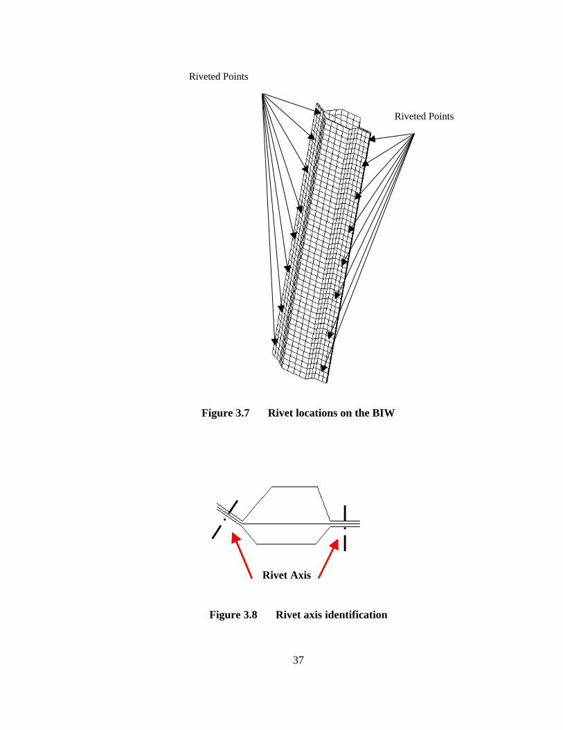
Modeling of the rivets that connect the BIW panels is based on defining the nodes

lying on the axis of the rivet (one each on inner, center, and outer) as a rigid body. This

option in LSDYNA is called as *CONSTRAINED_NODAL_RIGID_BODY and does

not consider failure of the rivets, if any, during the impact. Riveted locations on the

panels are as shown in Figure 3.7. Figure 3.8 shows a top view highlighting the axis of

the rivets through the three panels.

37

Figure 3.7 Rivet locations on the BIW

Figure 3.8 Rivet axis identification

Riveted Points

Riveted Points

Rivet Axis

38

3.3 TRIM

The term trim is used for a component that encloses the BIW. It is used to satisfy

both the aesthetic as well as impact protection requirements. The trim has a smooth outer

surface visible to the occupant while the inner surface has attachment features such as

clip housing and clip. The function of the clips is to enable fixing of the trim on to the

BIW components. The clip-housings provide the necessary clearance between the BIW

and the inner surface of the trim.

In this work, three different trim designs, namely Trim Design-1, Trim Design-2,

and Trim Design-3 are considered for evaluation under impact conditions. All three trim

designs are meshed using shell elements with default element formulation available in

LSDYNA.

Trim design-1 is a simple semi-circular cross section enclosing the BIW as shown

in Figure 3.9a with the center of the semi-circle being closer to the door area to aid more

stopping distance along the impact direction. A uniform thickness of 2 mm is used for the

trim, clip housing, and clip. In Trim Design-2 and Trim Design-3, the stopping distance

is increased relative to the inner as shown in Figure 3.9b and Figure 3.9c.

39

Figure 3.9a Trim Design-1

Figure 3.9b Trim Design-2

Figure 3.9c Trim Design-3

Windshield Area

Door Area

Impact Direction

Doghouse

Clip

Increased Clearance Compared

to Trim Design-1

Increased Clearance

Compared to Trim Design-2

40

Two clips, one on each end of the trim, are modeled in all three trim designs to

attach the trim to BIW. Figure 3.10 shows an isometric view of Trim Design-1

identifying the two clips and clip-housings. Attachment between the clips and inner is

modeled by rigidly attaching the clip to the slot provided on the inner panel using

CONSTRAINED_NODAL_RIGID_BODY card available in LSDYNA. The total length

of the trim cross section is 250 mm (half of BIW) and is centered along the cross

sectional length of BIW as shown in Figure 3.11.

41

Figure 3.10 Isometric view of trim design to show clips and clip housing

Figure 3.11 Side view of Trim Design-1 showing impact point on trim

Clip housingsClips

42

3.4 COUNTERMEASURE

Countermeasure is a general term used for components that work in conjunction

with interior trim to influence the HIC(d). In this work, ribs integrated on the inside of

the trim are evaluated as a countermeasure. Figure 3.12 shows Trim Design-1 with ribs

built on the inner surface of trim. The ribs were meshed with shell elements with a

minimum of three elements across the depth to capture appropriate bending during

impact. A uniform thickness of 1 mm (50% of trim thickness) is used for the ribs.

To study the influence of two design variables, namely rib thickness and rib

depth, on HIC(d), six models were generated to account for three rib thickness and three

rib depths. The three rib thickness used were 0.5 mm, 1.0 mm, and 1.5 mm. The three

rib depths used were 6 mm, 9 mm, and 12 mm as shown in Figures 3.13a, b, and c.

During impact, large forces are transmitted from the ribs to the inner panel over a

small area of the edge of the ribs. To improve the force distribution, a finer mesh is

preferred on the ribs. To avoid an overall increase in the number of elements in the

model by trying to match the mesh densities on both the ribs and trim, the feature

*CONTACT_TIED_SHELL_EDGE_TO_SURFACE in LSDYNA is used. This

interface ties all degrees of motion of the slave node to the master segment simulating a

tied interface. This enables to have finer mesh densities on the ribs while having a coarser

mesh density on the trim thereby improving computational efficiency.

43

Figure 3.12 Trim Design-1 with ribs as a countermeasure

Ribs

44

Figure 3.13a Rib depth of 6 mm

Figure 3.13b Rib depth of 9 mm

Figure 3.13c Rib depth of 12 mm

Rib Depth

Measurement

Trim

Surface

Increasing Rib

45

CHAPTER 4 ANALYSIS

4.1 MATERIAL DEFINITIONS

4.1.1 FREE MOTION HEADFORM (FMH)

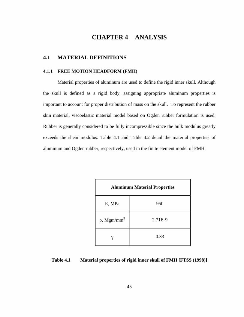
Material properties of aluminum are used to define the rigid inner skull. Although

the skull is defined as a rigid body, assigning appropriate aluminum properties is

important to account for proper distribution of mass on the skull. To represent the rubber

skin material, viscoelastic material model based on Ogden rubber formulation is used.

Rubber is generally considered to be fully incompressible since the bulk modulus greatly

exceeds the shear modulus. Table 4.1 and Table 4.2 detail the material properties of

aluminum and Ogden rubber, respectively, used in the finite element model of FMH.

Aluminum Material Properties

E, MPa 950

ρ, Mgm/mm3 2.71E-9

γ 0.33

Table 4.1 Material properties of rigid inner skull of FMH [FTSS (1998)]

46

Rubber Properties

ρ, Mgm/mm3 1.433E-9

Shear Modulus1, MPa -0.032

Shear Modulus 2, MPa 0.0838

Exponent 1 -8.384

Exponent 2 3.064

Shear Relaxation

Modulus, MPa

5.4

Table 4.2 Rubber skin material properties of FMH [FTSS (1998)]

47

4.1.2 BODY IN WHITE PANELS

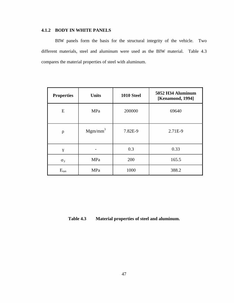
BIW panels form the basis for the structural integrity of the vehicle. Two

different materials, steel and aluminum were used as the BIW material. Table 4.3

compares the material properties of steel with aluminum.

Table 4.3 Material properties of steel and aluminum.

Properties Units 1010 Steel 5052 H34 Aluminum[Kenamond, 1994]

E MPa 200000 69640

ρ Mgm/mm3 7.82E-9 2.71E-9

γ - 0.3 0.33

σy MPa 200 165.5

Etan MPa 1000 388.2

48

4.1.3 TRIM AND RIBS

Trim material, PC/ABS, is modeled as being perfectly plastic using

*MAT_PIECEWISE_ELASTIC_PLASTIC (MAT 24) material model in LSDYNA. In

this material model, discrete points representing the plastic portion of the material are

defined using a load curve definition option such as *DEFINE_CURVE. To model a

perfectly plastic behavior, the slope between the yield point and the ultimate point is

given a very small number. Material model, *MAT_PIECEWISE_ELASTIC_PLASTIC,

allows user to specify a plastic strain based failure of the material. This option is used to

model the fracture of clip from clip housing during the impact and the fracture of the ribs.

A plastic failure strain of 50% is used. Table 4.4 shows the material properties of

PC/ABS used in this work.

PC/ABS properties

E, MPa 2350

ρ, Mgm/mm3 1.05E-9

γ 0.33

σy, MPa 70.3

σu, MPa 71.0

Table 4.4 Properties of PC/ABS [Sherman et al. (1995)]

49

4.2 IMPACT ANGLE SPECIFICATIONS

Before designing the trim to meet head impact protection, it is important to fully

understand the impact conditions specified by NHTSA. Several procedures outlined in

FMVSS 201 standards uniquely describe the targeting and impact methodology for each

specific target point. Knowledge of this procedure will help understand the significance

of design variables that can later be used in designing the interior components to provide

head impact protection. Some of the basic definitions and procedures are briefly

enumerated below.

4.2.1 HORIZONTAL APPROACH ANGLE

As an initial step in establishing the target points, the occupant head’s center of

gravity location in the vehicle coordinate system is determined based on the seating

reference point. This information needs to be identified for all the occupants in the

vehicle such as driver, passenger, and other occupants in the rear.

Determination of minimum and maximum horizontal approach angles for a given

trim design is shown in Figure 4.1. The figure shows the top view of the two occupants,

driver and passenger, and the cross section of the A-pillar. The line forming the shortest

distance between the driver head’s center of gravity point and the trim design is called as

the minimum horizontal angle measured from the negative x-axis in the counter

clockwise direction. The maximum horizontal approach angle is determined by

establishing the shortest distance to the A-pillar trim from the passenger head’s center of

gravity.

50

Figure 4.1 Determination of horizontal approach angles for an A-Pillar

x

-yDriver head’s

Center Of Gravity,

Passenger head’s

Center Of Gravity,

-x

Min Approach Angle

Max Approach Angle

Shortest Distance

A-Pillar

Front Of Vehicle

51

These angles are dependent on the interior trim design and on the occupant head’s

center of gravity relative to the trim. FMH is then launched along the horizontal angle

that may be in between the minimum and maximum values including the extreme angles.

In this work, the horizontal approach angle is referenced from the flange of the

inner panel rather than the negative x-axis as shown in Figure 4.1. This is done as a

matter of convenience so as to state the FMH impact angle off the flange of the inner

panel. Therefore a sum of 180° needs to be added to this angle to state the horizontal

approach angle as per NHTSA specifications. In this research, the analyses are

performed at two different horizontal approach angles measured from the flange of the

inner panel. These two angles are 30o (minimum) and 60o (maximum) (if stated as per

NHTSA definitions, these angles would be 210° and 240° respectively). The 30o

horizontal impact angle shown in Figure 4.2a, represents the impact vector passing

through the driver side occupant head’s center of gravity and forms a worst case since the

headform directly impacts the flange of the BIW. The 60o horizontal impact angle as

shown in Figure 4.2b, represents the impact vector passing through the passenger side

occupant head’s center of gravity. Figures 4.3a, 4.3b, and 4.3c, show the 30o horizontal

approach angle setup for the three different trim designs.

52

Figure4.2a Modified 300 Horizontal approach angle set up

Figure 4.2b Modified 60O Horizontal approach angle set up

30o

60o

x

y

Vehicle Front

Vehicle Rear

BIW flange

53

Figure4.3a 300 Horizontal approach angle set up for Trim Design-1

Figure4.3b 300 Horizontal approach angle set up for Trim Design-2

Figure4.3c 300 Horizontal Approach Angle Set Up for Trim Design-3

54

4.2.2 VERTICAL APPROACH ANGLE

Vertical approach angle is defined as the angle that the centerline of FMH makes

with x-y plane of the vehicle. Vertical approach angle is dependent on the target point

and a particular value of the horizontal approach angle. Figure 4.4 shows the three steps

needed to determine the vertical approach angle of the headform for a given target point

and horizontal angle for an A-Pillar. After identifying a particular target point on the

interior trim, the headform is first placed corresponding to any desired horizontal

approach angle as shown in step 1. The headform is then rotated about the xy-plane

towards the interior trim surface until the chin of the headform touches the trim as shown

in step 2. As a final step, the headform is rotated back 5o to achieve the vertical approach

angle.

In this research, a vertical approach angle of 15° is used for all the analyses as

shown in Figure 4.5.

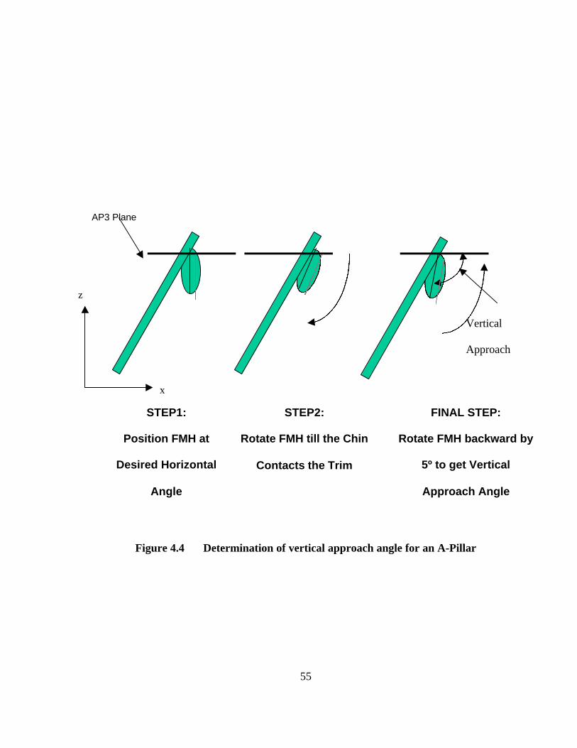
55

Figure 4.4 Determination of vertical approach angle for an A-Pillar

Vertical

Approach

AP3 Plane

STEP1:

Position FMH at

Desired Horizontal

Angle

STEP2:

Rotate FMH till the Chin

Contacts the Trim

FINAL STEP:

Rotate FMH backward by

5º to get Vertical

Approach Angle

x

z

56

Figure 4.5 Vertical approach angle of FMH

Vertical Approach

Angle = 15o

57

4.3 IMPACT POINT

Impact locations are determined based on NHTSA test procedures to identify

specific points in the vehicle and then determining the target planes on the pillars. These

measurements are unique to each vehicle model and require precise calculations relative

to the vehicle including the exact length and width of the interior roof area, height of the

pillars, and contour line measurements.

For an A-Pillar, there are three points (AP1, AP2, and AP3) that need to provide

head impact protection. The AP3 target point is a point on the AP3 cross-sectional plane

that gives the shortest distance between the driver side occupant head’ center of gravity

(in the forward most seating position) and the cross-section at AP3 as shown in Figure

4.6.

In this work the target point is measured at 45 mm from the edge of the flange

normal to the horizontal approach angle as shown in Figure 4.7.

58

Figure 4.6 Determination of target point for AP3 on the A-Pillar

AP2

Plane

AP3

Plane

Shortest

Distance

CG-F1-D

59

Figure 4.7 Target point used in current research

45 mm

Door Side Flange

60

4.4 IMPACT VELOCITY

Impact velocity is determined based on the presence of dynamic systems such as

air curtains embedded inside the side rail designed to deploy in an event of a side or roll-

over impact condition. Based on FMVSS 201 regulations, target points that fall with in

the deployed state of dynamic systems, should provide impact protection at a FMH

impact velocity of 12 mph while the remaining target points should be tested at 15 mph.

For vehicles without dynamic systems, all target locations should provide head impact

protection at 15 mph. In this work, all the analyses are performed at 15 mph as this forms

the worst case.

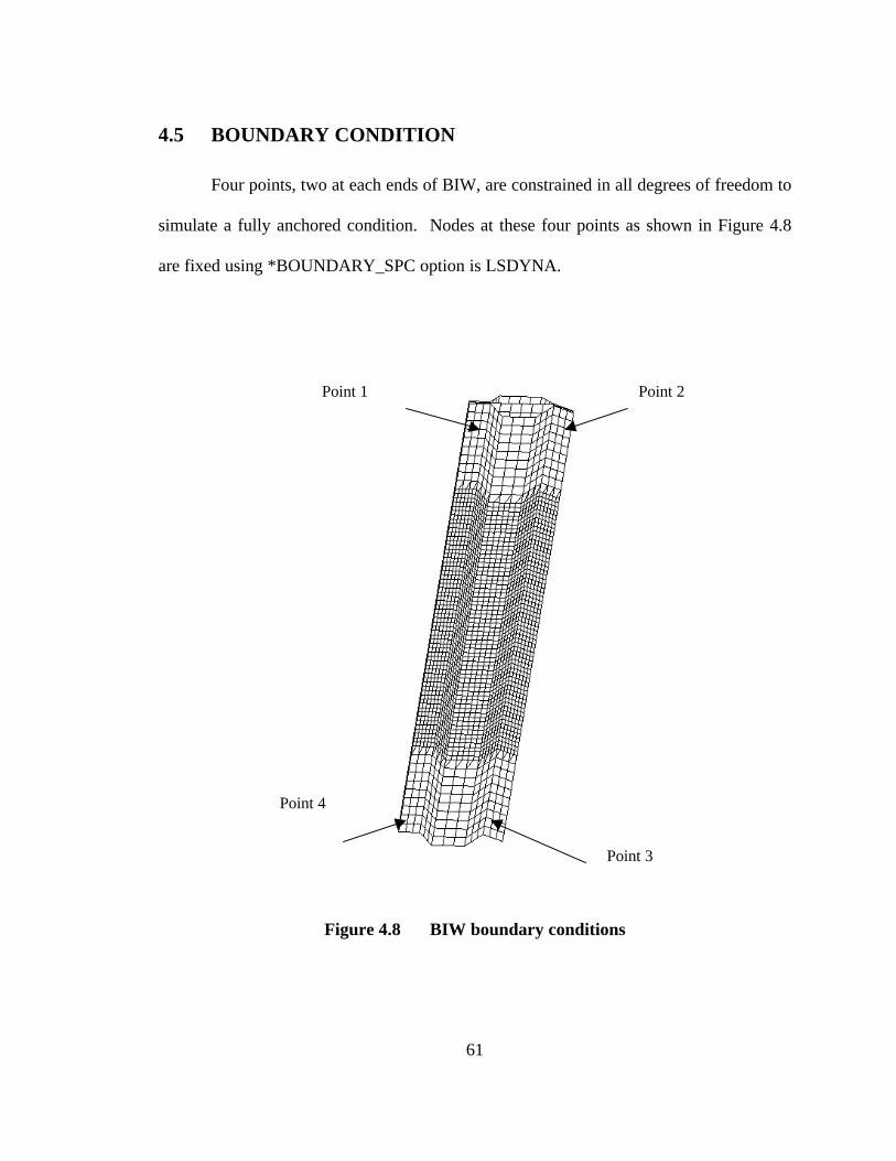
61

4.5 BOUNDARY CONDITION

Four points, two at each ends of BIW, are constrained in all degrees of freedom to

simulate a fully anchored condition. Nodes at these four points as shown in Figure 4.8

are fixed using *BOUNDARY_SPC option is LSDYNA.

Figure 4.8 BIW boundary conditions

Point 1 Point 2

Point 3

Point 4

62

4.6 TREATMENT OF CONTACT

Contact treatment between headform and the upper interior components during

impact is one of the most important factors influencing the acceleration response of the

headform. Choosing the appropriate contact algorithm and other contact parameters such

as friction can cause significant differences obtained in the acceleration pulse. In the

following sections, the treatment of contact between different components is discussed.

4.6.1 FMH AND PANELS

During impact, the exterior rubber skin of FMH undergoes compression upon

contact with the interior trim and/or BIW, absorbing a small magnitude of impact energy.

Numerical simulations of contact behavior involve application of spring elements

between the nodes of impacting bodies and calculating the forces needed to avoid

penetration between the two bodies. The stiffness of the spring elements is derived from

the material properties and element size information of the bodies coming in contact.

Large differences in material properties between the trim and the rubber skin, leads to

insufficient spring stiffness leading to penetration problems resulting in non-physical

behavior. This is overcome by modeling a null layer of shell elements with a small

thickness over the solid elements of rubber skin and assigning material properties of

impacting bodies such as trim and BIW. These elements are used only in contact

treatment of impacting bodies.

Selection and evaluation of different contact algorithms in any finite element code

is important to understand their influence of the resulting acceleration response of FMH.

In this work two different types of contact algorithms are investigated, viz.,

63

*CONTACT_SURFACE_2_SURFACE and *CONTACT_AUTOMATIC_GENERAL.

In *CONTACT_SURACE_2_SURFACE, only the nodes of each elements are checked

for penetration against the impact body. This interface type does not consider the shell

edges of the impacting body and becomes very important when a sharp edge of BIW such

as a flange comes in contact with the FMH. The

*CONTACT_AUTOMATIC_GENERAL was developed to account for contact between

nodes and elements as well as between shell edge and element. Since only the mid plane

is considered in representing thin structural members, such as BIW panels, it becomes

meaningful to study the effects of thickness consideration in contact algorithms on the

resulting peak acceleration of FMH. Therefore the above two contact algorithms were

analyzed with and without the consideration of thickness offsets.

4.6.2 BIW PANELS

To account for the interaction between the panels,

*CONTACT_SINGLE_SURFACE with a frictional value of 0.2 was defined. In this

interface type all the nodes defined in the contact are checked for penetration with the

elements and then appropriate force is applied to these nodes to account for load transfer.

By default, this interface type considers thickness of the elements included in the contact

definition and projects the mid plane surface to half its thickness.

64

4.7 SUMMARY OF ANALYSIS SET UP

A total of more than 40 analyses involving different material properties, angle of

impact, trim designs, and rib designs were performed in this research. Figure 4.9 shows

the flow chart of the different analysis performed for both steel and aluminum as BIW

material.

Figure 4.9 Flow chart of analysis setup for both steel and aluminum

No Ribs Ribs

DESIGN1

No Ribs Ribs

DESIGN2

No Ribs

0.5mm

6mm 9mm 12mm

Rib Depth

1.0 1.5mm

Thickness

Ribs

DESIGN 3

With Trim BASELINE(No Trim)

Minimum Horizontal Approach Angle30 degrees

Baseline(No Trim)

No Ribs

0.5mm

6mm 9mm 12mm

Rib Depth

1.0 1.5mm

Thickness

Ribs

DESIGN 3

With Trim

Maximum Horizontal Approach Angle60 degrees

65

CHAPTER 5 RESULTS AND DISCUSSIONS

5.1 FMH CALIBRATION DROP TEST

In the calibration drop test, the head form is dropped on its forehead

impact zone from a height of 14.8 inches in a free fall on to a rigid surface. To eliminate

the computational time during the free fall, the FMH is moved close to the rigid surface

in the vertical direction as shown in Figure 5.1 and an initial velocity equal to gh2 ,

where h = 14.8 inches, is applied to the headform. The current calibration drop test

corridor for FMH, recommended by NHTSA, is to be between 225 and 275 g’s.

Figure 5.1 FMH calibration drop test set-up

Rigid

Surface

66

Figure 5.2 shows the peak resultant acceleration of the finite element head form

and the upper and lower corridors as specified by NHTSA. Here, the upper and lower

corridors are obtained by simply scaling the finite element model FMH’s acceleration

response to achieve the minimum and maximum resultant values of 225 g’s and 275 g’s

respectively. It can be observed from the figure, that the peak resultant acceleration of

FMH lies between the upper and lower corridor and is approximately equal to 250 g’s. It

can therefore be concluded that the finite element model of the head form can be used to

evaluate the head impact protection of interior trim components.

67

Figure 5.2 Peak resultant acceleration of FMH for calibration drop test

The peak value of the resultant acceleration has a significant importance while

performing correlation between the finite element analysis results and the physical

testing. This is because, in finite element models, the peak resultant acceleration of the

FMH obtained in calibration drop test is fixed and does not vary for different simulations.

During physical testing, NHTSA recommends that the head form be calibrated before

every test. The peak resultant acceleration of the physical head form model could vary

between these tests and still meet the NHTSA recommendation. This leads to a basic

difference in peak value between the physical and finite element model of the head form.

Therefore it is recommended to take into account the peak resultant acceleration of the

head form in the calibration drop test, before every physical testing of interior trim

components.

68

5.2 EFFECTS OF INNER PANEL MESH DENSITY ON HIC(d)

In a 30° horizontal approach angle impact condition, the headform comes in direct

contact with the flange edge of the inner panel. Although the mesh density of the inner

panel could be sufficient to provide a smooth stress distribution, it was found important

to study the effects of mesh density on contact forces and resulting head acceleration.

The two different mesh densities of the inner panel, analyzed using steel as the

BIW material produced different acceleration response as shown in Figure 5.3. As it can

be observed from the figure, the initial slope of the two curves is quite similar during the

first 2 ms. But after 2 ms, the coarse mesh produces a sharp spike and then the

acceleration seems to drop with small oscillations. The fine mesh on the other hand

produces a smoother response and shows two peak values instead of one as seen in the

coarse mesh. The first peak is due to the initial contact of the FMH on the flange edge

and the second peak is due to the contact with the flat portion of the inner panel. As a

result of this, the coarse mesh and the fine mesh predicted a HIC(d) of 1258 and 1291,

respectively, resulting in a difference of 2.5%.

Closer examination of the animation showed that in the coarse mesh, only a few

nodes coming in contact with FMH exerted large impact forces on the rubber solid

element causing the solid element to deform non-physically. This phenomenon can be

seen in a side view of the model as shown in Figure 5.4a and 5.4b. In the fine mesh,

more number of elements near the impact zone helped to distribute the impact forces over

larger number of nodes providing a smoother acceleration response.

69

Figure 5.3 Coarse vs fine mesh of inner panel for 30°°horizontal angle

70

Figure 5.4a Deformation plot at 3.5 ms using coarse mesh on the inner panel

Figure 5.4b Deformation plot at 3.5 ms using fine mesh on the inner panel

71

Though the percentage difference was around 5%, missing the phenomenon of

predicting two peaks in the acceleration response of FMH and providing a smoother

response was found critical.

To fully understand the simulation sequence, a section plane A-A, normal to the

extruded length of the inner panel was cut at the impact point as shown in Figure 5.5.

Top view of the analysis sequence for the finer mesh and at section A-A can be seen at 0,

4, and 8 ms, in Figure 5.6. The first and second peak in the acceleration response is

identified in these sequences.

Based on these results, it was concluded to use the finer mesh density of the inner

panel for all the remaining analyses.

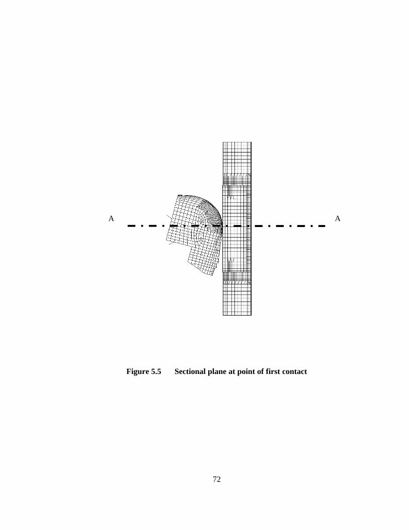
72

Figure 5.5 Sectional plane at point of first contact

A A

73

Figure 5.6 Baseline impact at 30°° horizontal approach angle

4 ms

0 ms

8 ms

Initial Peak

Second Peak

1ms

74

5.3 EVALUATION OF CONTACT ALGORITHMS

Using fine-mesh model of inner panel, the following three cases involving

different contact algorithms were analyzed at 30° horizontal approach angle.

1. *CONTACT_SURFACE_TO_SURFACE (without thickness offsets)

2. *CONTACT_SURFACE_TO_SURFACE (with thickness offsets)

3. *CONTACT_AUTOMATIC_GENERAL (with thickness offsets)

Figure 5.7 shows the resultant head acceleration obtained using

*CONTACT_SURFACE_TO_SURFACE contact type, with and without thickness

offsets. Although finer mesh density of the inner panel was used in both the analyses,

without considering thickness offsets in the treatment of contact produced oscillatory

response around peak acceleration levels. Also the phenomenon of two peaks were

missed without taking thickness offset into account resulting in a 5% decrease in HIC(d).

In Figure 5.8, the acceleration response using

*CONTACT_SURFACE_TO_SURFACE and *CONTACT_AUTOMATIC_GENERAL

is compared. Though *CONTACT_SURFACE_TO_SURFACE checks only the slave

nodes of the FMH for penetration and *CONTACT_AUTOMATIC_GENERAL checks

for both slave nodes and edges of elements for penetration, both contact algorithms

produced similar acceleration response. Smoother response of the acceleration pulse with

two peaks was observed in both the analyses. HIC(d) of 1291 and 1250 was predicted by

*CONTACT_SURFACE_TO_SURFACE and *CONTACT_AUTOMATIC_GENERAL

75

Figure 5.7 Effects of thickness consideration in contact algorithm

Figure 5.8 Comparison of contact algorithms

76

resulting in a 3.1% difference. This showed that having sufficient number of nodes on the

inner panel does not require treatment of element edges in contact algorithms. Based on

these results, it was concluded to use *CONTACT_SURFACE_TO_SURFACE with

thickness offsets in all the analyses.

77

5.4 BASELINE (NO TRIM) COMPARISON OF STEEL AND

ALUMINUM FOR 30°° AND 60°° HORIZONTAL APPROACH ANGLE

With the conclusions obtained from pervious results, performance between steel

and aluminum as a BIW material was investigated at 30° and 60° horizontal approach

angles and the results are presented in the following sections.

5.4.1 30°° HORIZONTAL APPROACH ANGLE

In this impact condition, both steel and aluminum showed unique energy

absorbing characteristics in the acceleration response of FMH as shown in Figure 5.9. As

discussed in previous section, the steel BIW showed two peaks in the acceleration pulse

and the difference between these two peaks was determined to be around 80 g’s. The

aluminum BIW, on the other had produced a more desirable acceleration response by

absorbing the impact energy at almost constant level of acceleration and having a

difference of only around 20 g’s between the two peaks. Also the time duration over

which the energy was absorbed in the case of aluminum was an additional 2 ms

compared to steel. Therefore using aluminum as a BIW material resulted in a smaller

HIC(d) of 967 while steel produced 1291.

5.4.2 60°° HORIZONTAL APPROACH ANGLE

For the 60° horizontal approach angle, the acceleration pulse using steel produced

an initial peak of around 180 g’s compared to 230 g’s in 30° impact angle as shown in

Figure 5.10. The second peak remained at around 160 g’s thereby indicating a difference

of only 20 g’s compared to 80 g’s between the first and second peak in 30° impact angle.

78

Figure 5.9 Steel vs aluminum for 30°°horizontal approach angle

Figure 5.10 Steel vs aluminum for 60°° horizontal approach angle

79

In the case of aluminum, a trend of increasing acceleration with an initial peak of

120 g’s at 2 ms and a maximum level of around 140 g’s at 4 ms is seen. The transient

plots, shown in Figure 5.11, indicate the initial contact of FMH to occur at point ‘B’ on

the inner panel rather than the flange edge as seen in 30° horizontal impact angle. This

resulted in a lesser initial peak and due to the deformation at point ‘B’ acceleration seems

to drop but increases quickly after contacting the flange edge. As in 30° impact angle,

the aluminum BIW produced a lesser HIC(d), 1051, as opposed to 1197 for steel BIW.

80

Figure 5.11 Transient plot for 60°° horizontal approach angle

0 ms

2 ms

4 ms

8 ms

Initial Contact at

Point ‘B’

Second Contact

with Flange

Deformation at

Point ‘B’

81


AND WITHOUT RIBS) AT 30°° HORIZONTAL APPROACH ANGLE

To compare the performance of steel and aluminum, Trim Design-1, with a semi-

circular cross section, was used, with and without ribs. Using the baseline model (no

trim), the trim was added and attached to the slot provided in the inner panel at the two

clip locations. The FMH was then moved along the impact vector to accommodate the

trim. As shown in Chapter 4, six layers of ribs with a constant thickness of 1mm and a

rib depth of 6 mm was used for the analysis involving Trim Design-1 with ribs. The rib

was attached to the trim by using *CONTACT_TIED_SHELL_EDGE-TO_SURFACE.

The results of Trim Design-1, with and without ribs, are discussed in the following

sections.

5.5.1 TRIM DESIGN-1 WITHOUT RIBS

In the cases of both steel and aluminum, using Trim Design-1 without ribs,

actually caused an increase in HIC(d) compared to baseline (no trim) analyses. By using

Trim Design-1 without ribs, steel and aluminum produced a HIC(d) of 1404 and 1139

respectively as shown in Figure 5.12. The baseline HIC(d) using steel and aluminum was

1291 and 967. Studying the acceleration pulse of steel, Trim Design-1 without ribs,

indeed eliminates the second peak in the acceleration pulse, but still resulted in an

increase in HIC(d). This was because more energy was absorbed by the inner panel at the

flange rather than by the trim, which seems to absorb energy only during initial 2 ms of

impact. Also less rotation of the FMH about the extruded length axis was observed

82

compared to the baseline analysis. The FMH then transfers the kinetic energy to the

BIW, starting at around 4 ms as shown in the transient plots in Figure 5.13.

Figure 5.12 Steel and aluminum using Trim Design-1 (without ribs) at 30°°horizontal Angle

83

Figure 5.13 Transient plots of steel using Trim Design-1 (without ribs) at 30°°horizontal approach angle

2 ms

0 ms

4 ms

6 ms

84

In the instance of aluminum, with Trim Design-1without ribs, the same

phenomenon is observed where the trim absorbs energy only during first couple of

milliseconds after contact. After the FMH impacts the flange, the peak acceleration

appears to be the same as seen in the baseline analysis at around 150 g’s. However a

higher second peak at 175 g’s is seen compared to 120 g’s in the baseline (no trim)

model.

5.5.2 TRIM DESIGN-1 WITH RIBS

Adding ribs to Trim Design-1 resulted in an increase in HIC(d) for both steel and

aluminum indicating a stiffer response. In the case of steel, the second peak in the

acceleration curves reappears as shown in Figure 5.14 due to the impact of ribs on the

BIW. Steel and aluminum using trim design, with ribs, produced a HIC(d) of 1416 and

1174, respectively, which is higher, compared to both the baseline and Trim Design-1

with ribs.

85

Figure 5.14 Steel and aluminum using Trim Design-1 (with Ribs) at 30°° horizontalapproach angle

86



In Trim Design-2, the clearance between the inner panel and the trim was

increased in an effort to reduce the HIC(d). And accordingly, the FMH was translated

back along the impact vector to accommodate the increase in the trim clearance with the

inner panel. As in Trim Design-1with ribs, 6 layers of ribs with 1 mm thickness and 6

mm of rib depth was attached to the inner surface of the trim. Results of Trim Design-2,

with and without ribs are presented in the following section.


By increasing the trim clearance in Trim Design-2, both steel and aluminum

produced HIC(d) values of 1318 and 1090, respectively, when compared with Trim

Design-1 value of 1404 and 1139, respectively as shown in Figure 5.15. This was

however, higher compared to the baseline (no trim) value of 1291 and 967.

In the case of steel, the peak value is slightly smaller compared to Trim Design-1

and the initial peak occurs at around 5 ms compared to 4 ms. In the transient plots shown

in Figure 5.16, the trims slips off the windshield flange at around 8 ms. However less

deformation of the inner panel is seen compared to Trim Design-1 at 8 ms indicating an

increase in the energy absorption by the trim.

Aluminum shows similar behavior as seen in Trim Design-1 except for the offsets

seen in the initial and second peaks of the acceleration pulse.

87

Figure 5.15 Steel and aluminum using Trim Design-2 (without ribs) at 30°°horizontal approach angle

88


0 ms

2 ms

4 ms

8 ms

89


Contrary to Trim Design-1, addition of ribs resulted in a reduction of HIC(d) for

both steel and aluminum as seen in Figure 5.17. Trim Design-2 with ribs produced

HIC(d) of 1233 and 974, respectively for steel and aluminum compared to 1318 and 1090

as seen in Trim Design-2 without ribs.

In the case of steel, there was a third level in the acceleration response at around 8

ms. This is because the ribs impact the inner panel at around 6 ms and absorbing energy

at constant acceleration until around 7 ms. Later, due to the buckling of the ribs the

acceleration starts to drop and finally the FMH bottoms out on the inner panel.

For the aluminum, the second peak in the acceleration pulse disappears and the

energy is absorbed at constant acceleration of around 150g’s indicating increased level of

energy absorption by the addition of ribs.

90

Figure 5.17 Steel and aluminum using Trim Design-2 (with ribs) at 30°° horizontalapproach angle

91



Trim Design-3 basically has a larger clearance with the inner panel, both along

the impact vector and along the clip axis. Also the trim edge on the windshield flange of

the inner panel was more curved to eliminate the edge slipping as seen in Trim Design-2.

Results of Trim Design-3, with and without ribs are discussed in the following sections.


Using Trim Design-3 without ribs, both steel and aluminum produced a lesser

HIC(d) values of 1270 and 902, respectively, which are the least among the analyses

considered. In the resultant acceleration plot for both steel and aluminum, shown in

Figure 5.18, a maximum time duration of around 4 ms was achieved before the FMH

impacted the flange of the inner panel. As a result of this, a lowest initial peak

acceleration of around 210 g’s was obtained in steel. And in the case of aluminum, even

without the addition of ribs, the second peak in the acceleration curve disappeared,

indicating increased level of energy absorption by the trim before the impact with the

flange of the inner panel. However, failure of the lower clip housing just before 8 ms

was seen in both steel and aluminum as shown in Figure 5.19. Failure criterion of the

clip housing was based on plastic strain and was set at 50% of strain in the material

model.

Modification to the trim edge on the windshield side of the inner flange resulted

in the trim staying on the flange longer than seen in Trim Design-2 resulting in increased

92

energy absorption of the trim. However, after 8 ms, slipping of the trim edge was seen in

the analysis.

Figure 5.18 Steel and aluminum using Trim Design-3 (without ribs) at 30°°horizontal approach Angle

93


Clip Housing

Impacting Inner

0 ms

2 ms

4 ms

8 ms

Trim Stays on

Windshield

flange

Failing of

Lower Clip

94


Addition of ribs with 1mm thickness and 6mm depth to Trim Design-3, resulted

in a further decrease in HIC(d) for the steel and aluminum. In both cases, failure of the

ribs was also seen. By adding ribs, the resultant acceleration in the case steel decreased

from 210g’s to 190g’s resulting in HIC(d) of 1163 as seen in Figure 5.20. There was

also a second peak due to the impact of ribs on the inner panel.

In the case of aluminum, the acceleration due to the impact of FMH with the inner

flange was further reduced to around 140g’s resulting in a HIC(d) of 829.

95

Figure 5.20 Steel and aluminum using Trim Design-3 (with ribs) at 30°° Horizontalapproach angle

96

Figure 5.21 and 5.22 show the resultant acceleration obtained from Trim Design-

1, Trim Design-2, and Trim Design-3, without ribs for steel and aluminum.

Figure 5.23 and 5.24 show the resultant acceleration obtained from Trim Design-

1, Trim Design-2, and Trim Design-3, with ribs for steel and aluminum.

97

Figure 5.21 Trim Design-1, 2, and 3 (without ribs) using aluminum at 30°°horizontal approach angle

Figure 5.22 Trim Design-1, 2, and 3 (without ribs) using steel at 30°° horizontalapproach angle

98

Figure 5.23 Trim Design-1, 2, and 3 (with ribs) using aluminum at 30°° horizontalapproach angle

Figure 5.24 Trim Design-1, 2, and 3 (with Ribs) using steel at 30°° horizontalapproach angle

99

5.8 TRIM DESIGN-3 WITH AND WITHOUT RIBS USING

ALUMINUM AT 60°° HORIZONTAL IMPACT ANGLE

Since Trim Design-3, with and without ribs, produced the best results compared

to all the previous analysis, it was then used to determine the effect of 60° horizontal

approach angle. Transient analysis results as seen in Figure 5.25 show that trim slips off

the inner flange on the door side at around 3 ms. This was followed by the trim edge

slipping from the windshield inner flange at 5 ms. Same phenomenon was observed in

both with and without ribs resulting in HIC(d) of 1119 and 970, respectively. Upon

investigation, it was later found that there would be weatherseal covering the inner flange

of the door side, which could prevent the trim slipping from the inner flange. On the

windshield flange, the windshield itself was not included in the analyses causing the trim

to slip off the flange. Inclusion of both these components could result in higher energy

absorption of the trim producing lesser HIC(d). However to establish a general

methodology in the design of A-Pillar trim cross-section, this was considered beyond the

scope of the project.

100

Figure 5.25 Transient plots of Trim Design-3 using aluminum at 60°° horizontalapproach angle

0 ms

3 ms

5 ms

7 ms

101

5.9 OPTIMUM TRIM OFFSET ESTIMATION

In the previous analyses involving different trim designs, it was seen that Trim

Design-3, with the integration of ribs provided the lowest HIC(d) of 829. Increasing the

offset helped to lower the HIC(d) level by enabling the trim to absorb more energy

before bottoming on the inner panel. However, to determine the optimum trim offset

distance, effects of trim clearance with corresponding values of HIC(d) need to be

established.

To achieve this the design of trim surface used in the present analyses is based on

three design parameters, viz., A, B, and C. These parameters are characterized relative to

BIW geometry and approach angles of the FMH. The definition of the three design

parameters based on the 30° impact angle is shown in Figure 5.26. Parameter ‘A’ is

defined to be the distance between the target point on the trim and the initial point of

contact between the trim and BIW measured along the impact vector. On the other hand,

‘B’ is defined to be the distance between the target point and the trim and the initial point

of contact between the trim and BIW measured normal to the inner flange surface.

Parameter ‘C’ is the distance between the inner panel and the trim surface along the clip

axis.

Tables 5.1 and 5.2 shows the values of the trim design variable ‘A’ for the three

trim designs and the corresponding HIC(d) values for both steel and aluminum.

102

Figure 5.26 Trim design variables definitions

Extreme point on the surface of the trim,measured normal to the inner panel surface

Impact Vector

A

BC

Fist Point Of Contact

103

STEEL

TRIM

DESIGN

DESIGN VARIABLE ‘A’

HIC(d),

Without Ribs

HIC(d),

With Ribs

1 -10.6 1404 1416

2 0.585 1318 1233

3 7.4 1270 1163

Table 5.1 Trim design variable ‘A’ and corresponding HIC(d) for steel at 30°°

horizontal approach angle

ALUMINUM

TRIM

DESIGN

DESIGN VARIABLE ‘A’

HIC(d),

Without Ribs

HIC(d),

With Ribs

1 -10.6 1139 1174

2 0.585 1090 974

3 7.4 902 830

Table 5.2 Trim design variable ‘A’ and corresponding HIC(d) for aluminum at

30°° horizontal approach angle

104

5.9.1 DEPENDENCE OF TRIM DESIGN VARIBLE ‘A’ ON HIC(d)

To establish the dependence of trim design variable ‘A’ on the HIC(d), results

obtained from analyzing the three trim designs, with and without ribs, are plotted against

the resulting HIC(d). Since the HIC(d) obtained in these component analyses could be

higher than that may actually be seen in the full vehicle analysis, percentage reduction in

HIC(d) for each trim design is plotted against the trim design variables. This can then be

used to estimate the trim offset depending on the desired percentage reduction in HIC(d)

obtained in the baseline (without trim) analysis of the full vehicle.

Figures 5.27 through 5.32 show the relationship between HIC(d) and the trim

design variable ‘A’, with and without ribs, at a 30° horizontal approach angle for both

steel and aluminum. Using these curves, an estimation of trim design variable, with and

without curves, can be achieved based on the desired percentage reduction in HIC(d).

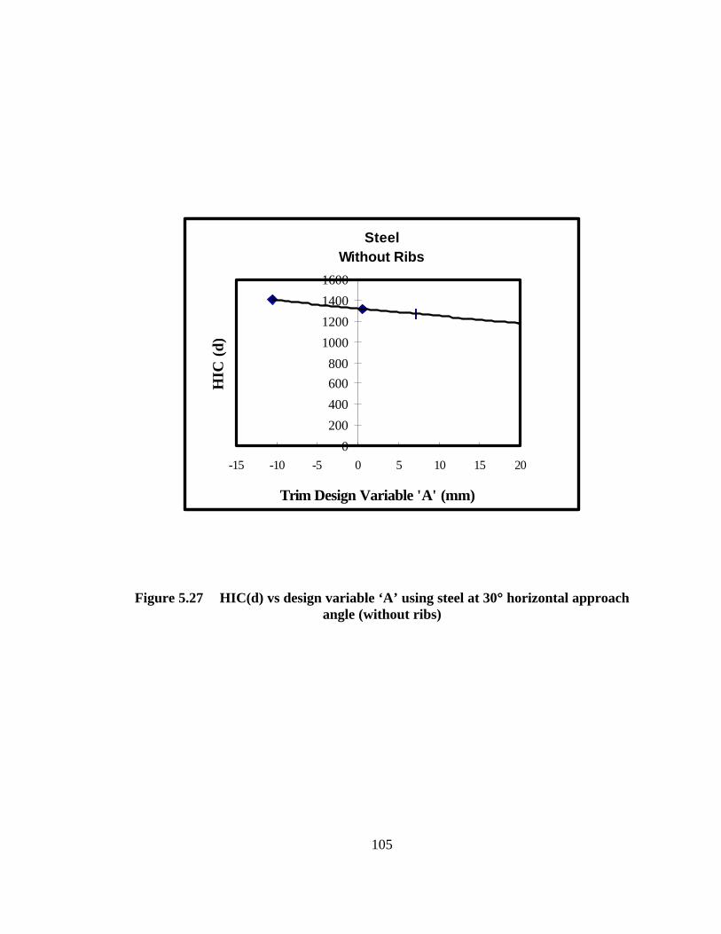
105

Figure 5.27 HIC(d) vs design variable ‘A’ using steel at 30°° horizontal approachangle (without ribs)

SteelWithout Ribs

0

200

400

600

800

1000

1200

1400

1600

-15 -10 -5 0 5 10 15 20

Trim Design Variable 'A' (mm)

HIC

(d)

106

Figure 5.28 HIC(d) vs design variable ‘A’ using aluminum at 30°° horizontalapproach angle (without ribs)

Figure 5.29 Percentage reduction in HIC(d) vs design variable ‘A’ using steel at30°° horizontal approach angle (without ribs)

AluminumWithout Ribs

0

200

400

600

800

1000

1200

1400

-15 -10 -5 0 5 10 15


HIC

(d)

SteelWithout Ribs

0

20

40

60

80

100

120

-15 -10 -5 0 5 10 15


% R

educ

tion

in H

IC(d

)

107

Figure 5.30 Percentage reduction in HIC(d) vs design variable ‘A’ usingaluminum at 30°° horizontal approach angle (without ribs)


0

20

40

60

80

100

120

-15 -10 -5 0 5 10 15Trim Design Variable 'A' (mm)

% R

educ

tion

in

HIC

(d)

108

Figure 5.31 Percentage reduction in HIC(d) vs design variable ‘A’ usingaluminum at 30°° horizontal approach angle (with ribs)

Figure 5.32 Percentage reduction in HIC(d) vs design variable ‘A’ usingaluminum at 30°° horizontal approach angle (with ribs)

AluminumWith Ribs

0

20

40

60

80

100

120

-15 -10 -5 0 5 10 15Trim Design Variable 'A' (mm)

% R

educ

tion

in

HIC

(d)

SteelWithRibs

0

20

40

60

80

100

120

-15 -10 -5 0 5 10 15


% R

educ

tion

in H

IC(d

)

109

5.9.2 DEPENDENCE OF TRIM DESIGN VARIABLE ‘B’ ON HIC(d)

In Table 5.3 and Table 5.4, the values of trim design variable ‘B’ for the three

trim designs and the corresponding HIC(d) values are tabulated for both steel and

aluminum, with and without ribs as the countermeasure.

Using these values, the trim design variable ‘B’ is plotted against percentage

reduction in HIC(d) in Figures 5.33 through 5. 36.

110

STEEL

TRIM

DESIGN

DESIGN VARIABLE ‘B’

HIC(d),

Without Ribs

HIC(d),

With Ribs

1 16 1404 1416

2 21 1318 1233

3 26 1270 1163

Table 5.3 Trim design variable ‘B’ and corresponding HIC(d) for steel at 30°°


ALUMINUM

TRIM

DESIGN

DESIGN VARIABLE ‘B’

HIC(d),

Without Ribs

HIC(d),

With Ribs

1 16 1139 1174

2 21 1090 974

3 26 902 830

Table 5.4 Trim design variable ‘B’ and corresponding HIC(d) for aluminum at


111

Figure 5.33 Percentage reduction in HIC(d) vs design variable ‘B’ using steel at30°° horizontal approach angle (without ribs)

Figure 5.34 Percentage reduction in HIC(d) vs design variable ‘B’ usingaluminum at 30°° horizontal approach angle (without ribs)

SteelWithout Ribs

70

78

86

94

102

110

15 20 25 30

Trim Design Variable 'B' (mm)

% R

educ

tion

in H

IC (

d)

Aluminum Without Ribs

0

20

40

60

80

100

120

15 20 25 30Trim Design Variable 'B' (mm)

% R

educ

tion

in H

IC

(d)

112

Figure 5.35 Percentage reduction in HIC(d) vs design variable ‘B’ using steel at30°° horizontal approach angle (with ribs)

Figure 5.36 Percentage reduction in HIC(d) vs design variable ‘B’ usingaluminum at 30°° horizontal approach angle (with ribs)

SteelWith Ribs

70

78

86

94

102

110

15 18 21 24 27

Trim Design Variable 'B' (mm)

% R

educ

tion

in H

IC (

d)

Aluminum With Ribs

0

20

40

60

80

100

120

15 20 25 30Trim Design Variable 'B' (mm)

% R

educ

tion

in H

IC (

d)

113

5.9.3 DEPENDENCE OF TRIM DESIGN VARIABLE ‘C’ ON HIC(d)

In Table 5.5 and 5.6, values of trim design variable ‘C’ for the three trim designs

and the corresponding HIC(d), with and without ribs, are tabulated for both steel and

aluminum as the BIW material.

Figures 5.37 though 5.39 shows the relationship between trim design variable ‘C’

and the corresponding percentage reduction in HIC(d).

114

STEEL

TRIM

DESIGN

DESIGN VARIABLE ‘C’

HIC(d),

Without Ribs

HIC(d),

With Ribs

1 33.8 1404 1416

2 37.5 1318 1233

3 42 1270 1163

Table 5.5 Trim design variable ‘C’ and corresponding HIC(d) for steel at 30°°


ALUMINUM

TRIM

DESIGN

DESIGN VARIABLE ‘C’

HIC(d),

Without Ribs

HIC(d),

With Ribs

1 33.8 1139 1174

2 37.5 1090 974

3 42 902 830

Table 5.6 Trim design variable ‘C’ and corresponding HIC(d) for aluminum at


115

Figure 5.37 Percentage reduction in HIC(d) vs design variable ‘C’ using steel at30°° horizontal approach angle (without ribs)

Figure 5.38 Percentage reduction in HIC(d) vs design variable ‘C’ using steel at30°° horizontal approach angle (with ribs)

SteelWithout Ribs

88

90

92

94

96

98

100

102

30 35 40 45Trim Design Variable 'C' (mm)

% R

educ

tion

in H

IC

(d)

SteelWith Ribs

0

20

40

60

80

100

120


% R

educ

tion

in H

IC

(d)

116

Figure 5.39 Percentage reduction in HIC(d) vs design variable ‘C’ usingaluminum at 30°° horizontal approach angle (without ribs)

Figure 5.40 Percentage reduction in HIC(d) vs design variable ‘C’ usingaluminum at 30°° horizontal approach angle (without ribs)

AluminumWith Ribs

0

20

40

60

80

100

120


% R

educ

tion

in H

IC

(d)


020406080

100120

30 35 40 45

Trim Design Variable 'C' (mm)

% R

educ

tion

in H

IC

(d)

117

5.10 DEPENDENCE OF RIB DESIGN VARIABLES ON HIC(d)

In all the previous analyses, a constant rib thickness of 1 mm and a constant rib

depth of 6 mm was used to compare the performance of rib as a countermeasure.

However, to optimize the rib structure by itself, it was important to study the effects of

different rib depths and rib thickness. To study these effects, Trim Design-3 was

considered as a basis for the analyses. In this research, three rib thickness of 0.5mm,

1.0mm, and 1.5mm were studied.

5.10.1 RIB THICKNESS

Figure 5.41 shows the HIC(d) obtained from this three rib thickness for Trim

Design-3 at 60° horizontal approach angle. As it can be seen in the figure, the HIC(d)

obtained decreases by increasing the thickness of the ribs. However, at around 1.5mm,

the HIC(d) seems to reach a plateau indicating no further reduction in HIC(d).

Figure 5.42 shows the HIC(d) plotted against the rib depth for a 30° horizontal

approach angle. In this angle of impact, the HIC(d) decreases initially from 0.5mm to

1mm and then starts to increase at 1.5mm indicating stiffening effect of the ribs. This

information would be very useful to prevent over stiffening of the rib structure and to

choose the right rib thickness that may result in a reduction in HIC(d) for any given angle

of impact.

118

Figure 5.41 Rib thickness vs HIC(d) for 60°° horizontal approach angle

Figure 5.42 Rib thickness vs HIC(d) for 30°° horizontal approach angle

863

829 839

500

600

700

800

900

1000

0 0.5 1 1.5 2

RIB THICKNESS, mm

HIC

(d)

953

898

871

800

900

1000

1100

0 0.5 1 1.5 2

RIB THICKNESS, mm

HIC

(d)

119

5.10.2 RIB DEPTH

To determine the effects of rib depth, three depths of 6 mm, 9 mm, and 12 mm

were analyzed using Trim Design-3 at 30° and 60° horizontal approach angles using

aluminum as BIW material.

Figure 4.43 and Figure 4.44 shows HIC(d) variation relative to the three rib

depths analyzed for both 60° and 30° horizontal approach angles respectively. As it can

be observed from the figures, for both cases, the HIC(d) decreases with increase in rib

depth and reaches a plateau beyond a depth of 12mm indication an optimum level.

120

Figure 5.43 Rib depth vs HIC(d) for 60°° horizontal approach angle

Figure 5.44 Rib depth vs HIC(d) for 30°° horizontal approach angle

898

776

721

500

600

700

800

900

1000

1100

1200

1300

0 2 4 6 8 10 12 14 16 18

RIB DEPTH, mm

HIC

(d)

829

776.1

744

500

600

700

800

900

1000

0 2 4 6 8 10 12 14 16 18

RIB DEPTH, mm

HIC

(d)

121

5.11 MODEL VALIDATION

In this research, a generic cross-section of an A-Pillar was used to determine the

effects of mesh density, contact algorithms and for determining the effects of HIC(d) for

various trim designs. Analysis performed on a similar approach for a particular program

(name of which cannot be furnished due to proprietary issues), excellent correlation was

achieved in acceleration response of the FMH and the HIC(d) was predicted within a

tolerance of 5%. By performing correlation with the physical test data, several contact

algorithms, material models, and other parameters were studied that affected the

correlation. This was conducted to identify factors that produced good agreement with

the experimental data and to use these correlated models to perform design iterations on

upper interior components.

122

CHAPTER 6 CONCLUSIONS, CONTRIBUTIONS, and

FUTURE WORK

6.1 CONCLUSIONS

The following conclusions are drawn from the various finite element analyses

performed in this research.

1. Analysis involving different contact algorithms showed a significant dependence of

the acceleration response on the type of contact algorithms employed in the

simulations. Even though a small change in HIC(d) was observed between different

contact algorithms, there was a considerable difference in the overall acceleration

response of the headform. Therefore, choosing the appropriate contact algorithm is

found to be very important in performing head impact simulations. In this work,

*CONTACT_SURFACE_2_SURFACE proved to be simple and reliable contact

algorithm in LSDYNA.

2. Inclusion and exclusion of thickness offsets in contact treatment produced significant

difference in the acceleration response for a particular contact algorithm while it

produced negligible difference for another contact algorithm. In comparing the time

event between the acceleration response and the animation sequence, consideration of

thickness offsets in contact algorithms was found to be crucial in achieving the

correct acceleration response of FMH.

3. In the comparison involving steel and aluminum as the BIW material, aluminum

showed good energy absorbing characteristics for the same A-Pillar cross-section. A

123

smoother deceleration history of FMH with reduced HIC(d) was observed in the case

of aluminum, which is beneficial. However, the performance of aluminum for a

given cross-section needs to be verified for other structural requirements such as side

and rollover impact conditions.

4. In analyzing three different trim designs, a greater trim offset was required for steel

compared with aluminum as the BIW material.

5. Failure of clips is found to be very crucial in the energy absorbing performance of the

trim. In this work, inclusion of failure of clips in the analysis resulted in higher

HIC(d) compared to clips that were modeled as a rigid connection. The inclusion of

clip failure in finite element modeling is important in predicting the correct energy

absorbing capacity.

6. For smaller trim offsets, addition of ribs produced an increase in HIC(d) while for

large trim offsets, ribs caused a decrease in HIC(d).

7. Rib thickness and rib depths for a particular trim can be effectively used to achieve

optimum reduction in HIC(d).

6.2 CONTRIBUTIONS

This research has established a direct comparison between steel and aluminum

under head impact conditions which is not found in earlier published work relating to

aluminum as a possible BIW material to meet head impact requirements. Further, this

work establishes a simple and efficient methodology, based on highly nonlinear resultant

acceleration response of the free motion headform, that can be applied to provide trim

offset recommendations.

124

6.3 FUTURE WORK

Future work that may be performed to continue the research conducted in this

work are listed below:

• Comparison of several types of energy absorbing foams with ribs as a

countermeasure.

• Study the effects of adhesive in addition to rivets for the attachment of BIW panels.

This can be useful to maintain the structural integrity of aluminum panels for other

impact conditions.

• Perform full vehicle analysis and determine the percentage reduction in HIC(d) for

different trim offsets to compare with the values obtained in this work.

• Evaluate different trim materials to determine the influence of material properties on

HIC(d).

• Establish similar methodologies for other impact locations on the upper interior

components of the vehicle.

125

CHAPTER 7 REFERENCES

1. Arimoto, H., Yasuki, T., Kawamura, K., Kondou, M., A Study on Energy

Absorbing Mechanism of Plastic Ribs, SAE Paper Number-982346, 1998.

2. Amori, T. R., Armitage, R. R., Chou, C. C., Lim, G. G., Patel R. N., Shahab S. A.,

Influence of System Variables on Interior Head Impact Testing, SAE Paper

Number-950882, 1995.

3. Bathe, K. J. and Wilson, E. L., Numerical Methods in Finite Element Analysis,

Prentice-Hall, 1976.

4. Burton D. E., Physics and Numerics of the TENSOR Code, Lawrence Livermore

National Laboratory, Internal Document, UCID-19428, 1982.

5. Chen, W. F. and Han, D. J., Plasticity or Structural Engineers, Springer-Verlag,

1988.

6. Chou, C. C. and Nyquist, G. W., Analytical Studies of the Head Injury Criterion

(HIC), SAE Paper Number-740082, 1974.

7. Chou, C. C., Zhao, Y., Lim, G. G., Patel, R. N. , Shahab, S. A. , and Patel, P. J. ,

Comparitive Analysis of Different Energy Absorbing Materials for Interior Head

Impact, SAE Paper Number-950332, 1995.

8. Collatz, L., The Numerical Treatment of Differential Equations, 1950.

9. Cook, R. D., Malkus, D S., Plesha, M E., Concepts and Applications of Finite

Element Analysis, 1989.

10. Crandall, R.W. and Graham, J. D., The effect of economy standards on automotive

safety, The Journal of Law and Economics, 1989.

126

11. First Technology Safety Systems (FTSS), Finite Element Model of FMH, 1998.

12. Gadd, C. W., Use of Weighted-Impulse Criterion for Estimating Injury Hazard,

Paper 660793-Proceedings of Tenth Stapp Car Crash Conference, P-12, New

York: Society of Automotive Engineer, Inc., 1966.

13. Gandhe, G. V., Lorenzo, L, and, Noritake, Y., Design Development of Energy

Absorbing Ribs for Meeting FMVSS 201 Extended Head Impact, Dow Chemicals

Co., Toyota Motor Corp., SAE Paper Number-970161, 1997.

14. John O. Hallquist, LSDYNA – Users Manual, 1998.

15. Hughes, T. J. R., Taylor, R. L., Sackman, J. L., Curnier, A. C., Kanoknukulchai,

W., A Finite Element Method for a Class of Contact-Impact Problems, 1976.

16. Kanianthra, J. N., Upper Head Impact Protection of Occupants in Real World

Crashes, 1995.

17. Kenamond, M., Evaluation of Aluminum Hexagonal Honeycomb Structures

Under Impact Loading, M. S. Thesis, West Virginia University, 1995.

18. Lim, G. G., Chou, C.C., Patel, R. N., Shahab, S. A., and Patel, P. J., Estimating

the Minimum Space to Meet Federal Interior Head Impact Protection, SAE Paper

Number-950333, 1995.

19. Lakshminarayan, V., Wang, H., Williams, W. J., Harajli, Y., and Chen, S.,

Application of CAE Nonlinear Crash Analysis to Aluminum Automotive

Crashworthiness Design, SAE Paper Number-951080, 1995.

20. National Highway Traffic Safety Administration, Standard No. 201: Head Impact

Protection: Final Rule’, 49 CFR, Parts 571, 572 and 589 [Docket No. 92098;

Notice 4], RIN 2127-AB85, Federal Motor Vehicle Safety Standards, Department

127

of Transportation, 1995.

21. Patrick, L. M., Lissner, H. R., and Gurdjian, E. S., Survival by Design-Head

Protection, Proceedings of Seventh Strapp Car Crash Conference, 1963.

22. Sawas , O., Brar, N. S., Dynamic Characterization of Compliant Materials using

All Polymeric Split Hopkinson Bar, SAE Paper Number-981138, 1998.

23. Sherman, K. C., Clark, C., Rawson J., Frost, C., Use of High Strain Rate Material

Data for Predicting Head Impact Performance of Thermoplastic, SAE Paper

Number-950331, 1995.

24. Traugott, T. and Maurer, M., New Ductile, Heat Resistant ABS Resin for Energy

Manangement Applications, SAE Paper Number-980969, 1998.

25. Walley, S. M. and Field, J. E., Strain Rate Sensitivity of Polymers, DYMAT

Journal, 1, No 3, 211, 1994.

26. Wilkins, M. L., Calculations of Elastic-Plastic Flow, 1964.

head impact characterization of generic a-pillar of an

Documents