have individual stocks become more volatile? an empirical...

Have Individual Stocks Become More Volatile? An Empirical Exploration ofIdiosyncratic Risk

John Y. Campbell; Martin Lettau; Burton G. Malkiel; Yexiao Xu

The Journal of Finance, Vol. 56, No. 1. (Feb., 2001), pp. 1-43.

Stable URL:

http://links.jstor.org/sici?sici=0022-1082%28200102%2956%3A1%3C1%3AHISBMV%3E2.0.CO%3B2-7

The Journal of Finance is currently published by American Finance Association.

Your use of the JSTOR archive indicates your acceptance of JSTOR's Terms and Conditions of Use, available athttp://www.jstor.org/about/terms.html. JSTOR's Terms and Conditions of Use provides, in part, that unless you have obtainedprior permission, you may not download an entire issue of a journal or multiple copies of articles, and you may use content inthe JSTOR archive only for your personal, non-commercial use.

Please contact the publisher regarding any further use of this work. Publisher contact information may be obtained athttp://www.jstor.org/journals/afina.html.

Each copy of any part of a JSTOR transmission must contain the same copyright notice that appears on the screen or printedpage of such transmission.

JSTOR is an independent not-for-profit organization dedicated to and preserving a digital archive of scholarly journals. Formore information regarding JSTOR, please contact [email protected].

http://www.jstor.orgMon Apr 2 13:42:13 2007

http://links.jstor.org/sici?sici=0022-1082%28200102%2956%3A1%3C1%3AHISBMV%3E2.0.CO%3B2-7

http://www.jstor.org/about/terms.html

http://www.jstor.org/journals/afina.html

THE JOURNAL OF FINANCE VOL. LVI, NO. 1 FEBRUARY 2001

Have Individual Stocks Become More Volatile? An Empirical Exploration of Idiosyncratic Risk

JOHN Y. CAMPBELL, MARTIN LETTAU, BURTON G. MALKIEL, and YEXIAO XU*

ABSTRACT

This paper uses a disaggregated approach to study the volatility of common stocks a t the market, industry, and firm levels. Over the period from 1962 to 1997 there has been a noticeable increase in firm-level volatility relative to market volatility. Accordingly, correlations among individual stocks and the explanatory power of the market model for a typical stock have declined, whereas the number of stocks needed to achieve a given level of diversification has increased. All the volatility measures move together countercyclically and help to predict GDP growth. Market volatility tends to lead the other volatility series. Factors that may be responsible for these findings are suggested.

IT IS BY NOW A COMMONPLACE OBSERVATION that the volatility of the aggregate stock market is not constant, but changes over time. Economists have built increasingly sophisticated statistical models to capture this time variation in volatility. Simple filters such as the rolling standard deviation used by Officer (1973) have given way to parametric ARCH or stochastic-volatility models. Partial surveys of the enormous literature on these models are given by Bollerslev, Chou, and Kroner (1992), Hentschel (1995), Ghysels, Harvey, and Renault (1996), and Campbell, Lo, and MacKinlay (1997, Chapter 12).

Aggregate volatility is, of course, important in almost any theory of risk and return, and it is the volatility experienced by holders of aggregate index funds. But the aggregate market return is only one component of the return to an individual stock. Industry-level and idiosyncratic firm-level shocks are also important components of individual stock returns. There are several reasons to be interested in the volatilities of these components.

* John Y. Campbell is a t Harvard University, Department of Economics and NBER; Lettau is a t the Federal Reserve Bank of New York and CEPR; Malkiel is a t Princeton University; and Xu is a t the University of Texas at Dallas. This paper merges two independent projects, Camp-bell and Lettau (1999) and Malkiel and Xu (1999). Campbell and Lettau are grateful to Sang-joon Kim for his contributions to the first version of their paper, Campbell, Kim, and Lettau (1994). We thank two anonymous referees and Ren6 Stulz for useful comments and Benjamin Zhang for pointing out an error in a previous draft. Jung-Wook Kim and Matt Van Vlack pro-vided able research assistance. The views are those of the authors and do not necessarily reflect those of the Federal Reserve Bank of New York or the Federal Reserve System. Any errors and omissions are the responsibility of the authors.

2 The Journal o f Finance

First, many investors have large holdings of individual stocks; they may fail to diversify in the manner recommended by financial theory, or their holdings may be restricted by corporate compensation policies. These investors are affected by shifts in industry-level and idiosyncratic volatility, just as much as by shifts in market volatility. Second, some investors who do try to diversify do so by holding a portfolio of 20 or 30 stocks. Conventional wisdom holds that such a portfolio closely approximates a well-diversified portfolio in which all idiosyncratic risk is eliminated. However, the adequacy of this approximation depends on the level of idiosyncratic volatility in the stocks making up the portfolio. Third, arbitrageurs who trade to exploit the mispricing of an individual stock (as opposed to a pattern of mispricing across many stocks) face risks that are related to idiosyncratic return volatility, not aggregate market volatility. Larger pricing errors are possible when idiosyncratic firm-level volatility is high (Ingersoll (1987), Chapter 7, Shleifer and Vishny (1997)). Fourth, firm-level volatility is important in event studies. Events affect individual stocks, and the statistical significance of abnormal event-related returns is determined by the volatility of individual stock returns relative to the market or industry (Campbell et al. (1997), Chapter 4). Finally, the price of an option on an individual stock depends on the total volatility of the stock return, including industry-level and idiosyncratic volatility as well as market volatility.

Disaggregated volatility measures also have important relations with aggregate output in some macroeconomic models. Models of sectoral reallocation, following Lilien (1982), imply that an increase in the industry-level volatility of productivity growth may reduce output as resources are di- verted from production to costly reallocation across sectors. Models of "cleansing recessions" (Caballero and Hammour (1994), Eden and Jovanovic (1994)) emphasize similar effects at the level of the firm. An exogenous increase in the arrival rate of information about management quality may temporarily reduce output as resources are reallocated from low-quality to high-quality firms; alternatively, a recession that occurs for some other reason may re- veal information about management quality and increase the pace of reallocation across firms.

There is surprisingly little empirical research on volatility at the level of the industry or firm. A few papers use disaggregated data to study the "leverage" effect, the tendency for volatility to rise following negative returns (Black (1976), Christie (1982), Duffee (1995)). Engle and Lee (1993) use a factor ARCH model to study the persistence properties of firm-level volatility for a few large stocks. Some researchers have used stock market data to test macroeconomic models of reallocation across industries or firms (Loun- gani, Rush, and Tave (1990), Bernard and Steigerwald (1993), Brainard and Cutler (1993)), or to explore the firm-level relation between volatility and investment (Leahy and Whited (1996)). Roll (1992) and Heston and Rouwen- horst (1994) decompose world market volatility into industry and country- specific effects and study the implications for international diversification. Bekaert and Harvey (1997) construct a measure of individual firm dispersion to study the volatility in emerging markets.

3 Have Individual Stocks Become More Volatile?

The purpose of this paper is to provide a simple summary of historical movements in market, industry, and firm-level volatility. We provide a decomposition of volatility that does not require the estimation of covariances or betas for industries or firms. In the interest of simplicity we follow Mer- ton (1980), Poterba and Summers (1986), French, Schwert, and Stambaugh (1987), Schwert (1989), and Schwert and Seguin (1990) and use daily data within each month to construct sample variances for that month, without imposing any parametric model to describe the evolution of variances over time. Multivariate volatility models are notoriously complicated and difficult to estimate. Furthermore, although the choice of a parametric model may be essential for volatility forecasting, it is less important for describing historical movements in volatility, because all models tend to produce historical fitted volatilities that move closely together. The reason for this was first given by Merton (1980) and was elaborated by Nelson (1992): with sufficiently high-frequency data, volatility can be estimated arbitrarily ac- curately over an arbitrarily short time interval. Recently Andersen et al. (1999) have used a similar approach to produce daily volatilities from intra- daily data on the prices of large individual stocks.

We first confirm and update Schwert's (1989) finding that market volatility has no significant trend using monthly data from 1926 to 1997. We next estimate market, industry, and firm-level variances using daily CRSP data ranging from 1962 to 1997. We find that market and industry variances have been fairly stable in that sample period also. However, firm-level variance displays a large and significant positive trend, more than doubling between 1962 and 1997. This finding is robust to plausible variations in our methodology, for example, downweighting the influence of the 1987 crash, fixing the number of firms in the sample, or using weekly or monthly returns instead of daily returns to estimate volatility. We conclude that, although the market as a whole has not become more volatile, uncertainty on the level of individual firms has increased substantially over a 35-year period. Consistent with this observation, we find declines over time in the correlations among individual stocks and in the explanatory power of the market model for a typical stock.

We also study the variations of the volatility measures around their long- term trends. The three volatility measures are positively correlated with each other as well as autocorrelated. Granger-causality tests suggest that market volatility tends to lead the other volatility series. All three volatility measures increase substantially in economic downturns and tend to lead recessions. The volatility measures-particularly industry-level volatility- help to forecast economic activity and reduce the significance of other com- monly used forecasting variables.

The paper is organized as follows. In Section I we present the basic decomposition of volatility into market, industry, and idiosyncratic components. Section I1 directly measures trends in volatility. In Section 111, we provide alternative indirect evidence of increased idiosyncratic volatility. Here we study correlations across individual stocks, the explanatory power of the market model for individual stocks, and the number of stocks needed to

4 The Journal o f Finance

achieve a given level of diversification. Section IV studies the lead-lag relations among our volatility measures as well as their cyclical properties. In Section V, we suggest some factors that may have influenced the apparent increase in idiosyncratic volatility. Section VI presents concluding comments.

I. Estimation of Volatility Components

A. Volatility Decomposition

We decompose the return on a "typical" stock into three components: the market-wide return, an industry-specific residual, and a firm-specific residual. Based on this return decomposition, we construct time series of volatility measures of the three components for a typical firm. Our goal is to define volatility measures that sum to the total return volatility of a typical firm, without having to keep track of covariances and without having to estimate betas for firms or industries. In this subsection, we discuss how we can achieve such a representation of volatility. The next subsection presents the estimation procedure and some details of the data sample.

Industries are denoted by an i subscript and individual firms are indexed by j. The simple excess return of firm j that belongs to industry i in period t is denoted as Rj,. This excess return, like all others in the paper, is measured as an excess return over the Treasury bill rate. Let wjitbe the weight of firm j in industry i . Our methodology is valid for any arbitrary weighting scheme provided that we compute the market return using the same weights; in this application we use market value weights. The excess return of industry i in period t is given by Rit = CjEi wjitRjit. Industries are aggregated correspondingly. The weight of industry i in the total market is denoted by wit,and the excess market return is Rmt = X i witRit.

The next step is the decomposition of firm and industry returns into the three components. We first write down a decomposition based on the CAPM, and we then modify it for empirical implementation. The CAPM implies that we can set intercepts to zero in the following equations:

for industry returns and

R.. = p..Rit+ 7.. J L ~ J l J l t

= Pji PimRmt + Pji zit qjit (2)

for individual firm returns.1 In equation (1) Pi, denotes the beta for industry i with respect to the market return, and E", is the industry-specific residual. Similarly, in equation (2) Pji is the beta of firm j in industry i with

'We could work with the market model, not imposing the mean restrictions of the CAPM, and allow free intercepts w i and wji in equations (1) and (2). However our goal is to avoid estimating firm-specific parameters; despite the well-known empirical deficiencies of the CAPM, we feel that the zero-intercept restriction is reasonable in this context.


respect to its industry, and ii,.,, is the firm-specific residual. qjq is orthogonal by construction to the industry return Rit;we assume that it is also orthogonal to the components Rmt and git. In other words, we assume that the beta of firm j with respect to the market, pjm, satisfies pjm = PjiPim. The weighted sums of the different betas equal unity:

2wit Pim = 1, 2wjit pji = 1.

The CAPM decomposition (1)and (2) guarantees that the different components of a firm's return are orthogonal to one another. Hence it permits a simple variance decomposition in which all covariance terms are zero:

The problem with this decomposition, however, is that it requires knowledge of firm-specific betas that are difficult to estimate and may well be unstable over time. Therefore we work with a simplified model that does not require any information about betas. We show that this model permits a variance decomposition similar to equations (4) and (5) on an appropriate aggregate level.

First, consider the following simplified industry return decomposition that drops the industry beta coefficient pi, from equation (1):

Equation (6) defines as the difference between the industry return Rit and the market return Rmt.Campbell et al. (1997, Chapter 4, p. 156) refer to equation (6) as a "market-adjusted-return model" in contrast to the market model of equation (1).

Comparing equations (1)and (6), we have

The market-adjusted-return residual equals the CAPM residual of equation (4) only if the industry beta pi, = l or the market return R,, = 0.

The apparent drawback of the decomposition (6) is that Rmtand eit are not orthogonal, and so one cannot ignore the covariance between them. Com- puting the variance of the industry return yields

6 The Journal of Finance

where taking account of the covariance term once again introduces the industry beta into the variance decomposition.

Note, however, that although the variance of an individual industry return contains covariance terms, the weighted average of variances across industries is free of the individual covariances:

xwit Var(Rit) = Var(Rmt)+ xwit Var(eit) i i

= sit + a;, (9)

where a;, = Var(R,,) and a; = Xi wit Var(eit). The terms involving betas aggregate out because from equation (3) Xi witpi, = 1.Therefore we can use the residual eit in equation (6) to construct a measure of average industry- level volatility that does not require any estimation of betas. The weighted average Xi w, Var(Rit) can be interpreted as the expected volatility of a randomly drawn industry (with the probability of drawing industry i equal to its weight wit).

We can proceed in the same fashion for individual firm returns. Consider a firm return decomposition that drops pji from equation (2):

where qj, is defined as

The variance of the firm return is

The weighted average of firm variances in industry i is therefore

where a;, = XjEiwjit Var(qjit) is the weighted average of firm-level volatility in industry i. Computing the weighted average across industries, using equation (9), yields again a beta-free variance decomposition:

witxwjit Var (Rjit) = xwit Var(Rit 1 + xwit 2Wjit Var(qjit i j € i i i j € i


where a$ = Xi wits$, = Xi witXjEiwjit Var(qjit) is the weighted average of firm-level volatility across all firms. As in the case of industry returns, the simplified decomposition of firm returns (10) yields a measure of average firm-level volatility that does not require estimation of betas.

We can gain further insight into the relation between our volatility decomposition and that based on the CAPM if we aggregate the latter (equations (4) and (5)) across industries and firms. When we do this we find that

where BE", = Xi wit Var(Cit) is the average variance of the CAPM industry shock Zit, and CSV, (Pi,) = Xi wit(Pi, - 1)' is the cross-sectional variance of industry betas across industries. Similarly,

where 5; = Xi witXjEiwjit Var(fjjit), CSVt(Pjm) = Xi witXj wjit(Pjm- 1)' is the cross-sectional variance of firm betas on the market across all firms in all industries, and CSVt(Pji) = Xi witXj wjit(Pji - 1)' is the cross-sectional variance of firm betas on industry shocks across all firms in all industries.

Equations (15) and (16) show that cross-sectional variation in betas can produce common movements in our variance components a:,, a;, and a;, even if the CAPM variance components 5; and 5;t do not move at all with the market variance a:,. We return to this issue in Section IV.A, where we show that realistic cross-sectional variation in betas has only small effects on the time-series movements of our volatility components.

B. Estimation

We use firm-level return data in the CRSP data set, including firms traded on the NYSE, the AMEX, and the Nasdaq, to estimate the volatility components in equation (14) based on the return decomposition (6) and (10). We aggregate individual firms into 49 industries according to the classification scheme in Fama and French (1997).2 We refer to their paper for the SIC classification. Our sample period runs from July 1962 to December 1997. Obviously, the composition of firms in individual industries has changed dramatically over the sample period. The total number of firms covered by the CRSP data set increased from 2,047 in July 1962 to 8,927 in December 1997. The industry with the most firms on average over the sample is Fi- nancial Services with 628 (increasing from 43 to 1,525 over the sample), and the industry with the fewest firms is Defense with 8 (increasing from 3 to 12 over the sample). Based on average market capitalization, the three largest

They actually use 48 industries, but we group the firms that are not covered in their scheme in an additional industry.


industries on average over the sample are Petroleum/Gas (11percent), Fi- nancial Services (7.8 percent) and Utilities (7.4 percent). Table 4 includes a list of the 10 largest industries. To get daily excess return, we subtract the 30-day T-bill return divided by the number of trading days in a month.

We use the following procedure to estimate the three volatility components in equation (14). Let s denote the interval at which returns are measured. We will use daily returns for most estimates but also consider weekly and monthly returns to check the sensitivity of our results with respect to the return interval. Using returns of interval s, we construct volatility estimates at intervals t. Unless otherwise noted, t refers to months. To estimate the variance components in equation (14) we use time-series variation of the individual return components within each period t. The sample volatility of the market return in period t, which we denote from now on as MKT,, is computed as

where ,urnis defined as the mean of the market return R,, over the sample.3 To be consistent with the methodology presented above, we construct the market returns as the weighted average using all firms in the sample in a given period. The weights are based on market capitalization. Although this market index differs slightly from the value-weighted index provided in the CRSP data set, the correlation is almost perfect at 0.997. For weights in period t we use the market capitalization of a firm in period t - 1and take the weights as constant within period t.

For volatility in industry i, we sum the squares of the industry-specific residual in equation (6) within a period t:

As shown above, we have to average over industries to ensure that the covariances of individual industries cancel out. This yields the following measure for average industry volatility IND,:

IND, = xwit$2,. (19) i

We also experimented with time-varying means but the results are almost identical. Foster and Nelson (1996)have recently provided a more comprehensive study of rolling regressions to estimate volatility. They show that under quite general conditions a two-sided rolling regression will be optimal. However, such a technique causes serious problems for the study of lead- lag relationships that is one focus of this paper.


Estimating firm-specific volatility is done in a similar way. First we sum the squares of the firm-specific residual in equation (10) for each firm in the sample:

Next, we compute the weighted average of the firm-specific volatilities within an industry:

And lastly we average over industries to obtain a measure of average firm- level volatility FIRM, as

FIRM, = t:wit$;,. (22) i

As with industry volatility, this procedure ensures that the firm-specific covariances cancel out.

11. Measuring Trends in Volatility

A. Graphical Analysis

Popular discussions of the stock market often suggest that the volatility of the market has increased over time. At the aggregate level, however, this is simply untrue. The percentage volatility of market index returns shows no systematic tendency to increase over time. To be sure, there have been epi- sodes of increased volatility, but they have not persisted. Schwert (1989) presented a particularly clear and forceful demonstration of this fact, and we begin by updating his analysis.

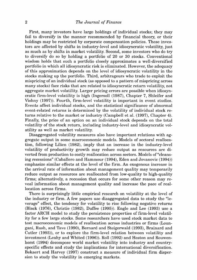
In Figure 1we plot the volatility of the value weighted NYSE/AMEX/ Nasdaq composite index for the period 1926 through 1997. For consistency with Schwert, we compute annual standard deviations based on monthly data. The figure shows the huge spikes in volatility during the late 1920s and 1930s as well as the higher levels of volatility during the oil and food shocks of the 1970s and the stock market crash of 1987. In general, however, there is no discernible trend in market volatility. The average annual standard deviation for the period from 1990 to 1997 is 11percent, which is actually lower than that for either the 1970s (14 percent) or the 1980s (16 percent).

These results raise the question of why the public has such a strong impres- sion of increased volatility. One possibility is that increased index levels have increased the volatility of absolute changes, measured in index points, and that the public does not understand the need to measure percentage returns. An-


0.0 1920 1930 1940 1950 1960 1970 1980 1990 2000

Date

Figure 1. Standard deviation of value-weighted stock index. The standard deviation of monthly returns within each year is shown for the period from 1926 to 1997.

other possibility is that public impressions are formed in part by the behavior of individual stocks rather than the market as a whole. Casual empiricism does suggest increasing volatility for individual stocks. On any specific day, the most volatile individual stocks move by extremely large percentages, often 25 percent or more. The question remains whether such impressions from casual empiricism can be documented rigorously and, if so, whether these patterns of volatility for individual stocks are different from those existing in earlier periods. With this motivation, we now present a graphical summary of the three volatility components described in the previous section.

Figures 2 to 4 plot the three variance components, estimated monthly, using daily data over the period from 1962 to 1997: market volatility MKT, industry-level volatility IND, and firm-level volatility FIRM. All three series are annualized (multiplied by 12). The top panels show the raw monthly time series and the bottom panels plot a lagged moving average of order 12. Note that the vertical scales differ in each figure and cannot be compared with Fig- ure 1(because we are now plotting variances rather than a standard deviation).

Market volatility shows the well-known patterns that have been studied in countless papers on the time variation of index return variances. Com- paring the monthly series with the smoothed version in the bottom panel suggests that market volatility has a slow-moving component along with a

Have Individual Stocks Become More Volatile?

Panel A. Market volatility

% % Z % e E R E R i % S Z % % 8 8 S

Panel B. Market volatility, MA(12)

Figure 2. Annualized market volatility MKT. The top panel shows the annualized variance within each month of daily market returns, calculated using equation (17), for the period July 1962 to December 1997. The bottom panel shows a backwards 12-month moving average of MKT. NBER-dated recessions are shaded in gray to illustrate cyclical movements in volatility.

fair amount of high-frequency noise. Market volatility was particularly high around 1970, in the mid-1970s, around 1980, and at the very end of the sample. The stock market crash in October 1987 caused an enormous spike in market volatility which is cut off in the plot. The value of MKT in October 1987 is 0.672, about six times as high as the second highest value. The plot also shows NBER-dated recessions shaded in gray. A casual look at the plot suggests that market volatility increases in recessions. We will study the cyclical behavior of MKT and the other volatility measures below.

Next, consider the behavior of industry volatility IND in Figure 3. Com-pared with market volatility, industry volatility is slightly lower on average. As for MKT, there is a slow-moving component and some high-frequency

8


Panel A. Industry volatility

5 2 $ 8 8 ? 2 R X i ? 8 % $ % 8 8 % g 8

Panel B. industry volatility, MA(12)

Figure 3. Annualized industry-level volatility IND. The top panel shows the annualized variance within each month of daily industry returns relative to the market, calculated using equations (18) and (19), for the period from July 1962 to December 1997. The bottom panel shows a backwards 12-month moving average of IND. NBER-dated recessions are shaded in gray to illustrate cyclical movements in volatility.

noise. IND was particularly high in the mid-1970s and around 1980. The effect of the crash in October 1987 is quite significant for IND, although not as much as for MKT. More generally, industry volatility seems to increase during macroeconomic downturns.

Figure 4 plots firm-level volatility FIRM. The first striking feature is that FIRM is on average much higher than MKT and IND. This implies that firm-specific volatility is the largest component of the total volatility of a n average firm. The second important characteristic of FIRM is that it trends up over the sample. The plots of MKT and IND do not exhibit any visible upward slope whereas for FIRM i t is clearly visible. This indicates that the


Panel A. Firm volatility

% % Z 8 E X t Z K R 8 % $ 5 % 8 % S

Panel B. Firm volatility, MA(12)

Figure 4. Annualized firm-level volatility FIRM. The top panel shows the annualized variance within each month of daily firm returns relative to the firm's industry, calculated using equations (20)-(22), for the period from July 1962 to December 1997. The bottom panel shows a backwards 12-month moving average of FIRM. NBER-dated recessions are shaded in gray to iIlustrate cyclicaI movements in volatility.

stock market has become more volatile over the sample but on a firm level instead of a market or industry level. Apart from the trend, the plot of FIRM looks similar to MKT and IND. Firm-level volatility seems to be higher in NBER-dated recessions and the crash also has a significant effect.

Looking at the three volatility plots together, it is clear that the different volatility measures tend to move together, particularly at lower frequencies. For example, all three volatility measures increase during the oil price shocks in the early to mid-1970s. However, there are also some periods in which the volatility measures move differently. For example, IND is very high compared to its long-term mean during the early 1980s while MKT and FIRM

8

The Journal of Finance

Table I Autocorrelation Structure

Raw Data Downweighted Crash

Autocorrelation MKT IND FIRM MKT IND FIRM

Note: This table reports the autocorrelation structure of monthly volatility measures con-structed from daily data. MKT is market volatility constructed from equation (17), IND is industry-level volatility constructed from equations (18) and (19), and FIRM is firm-level volatility constructed from equations (20)-(22). All measures are value-weighted variances. The columns denoted "downweighted c r a s h replace the observation in October 1987 with the second- largest observation in the respective series, pi denotes the i th monthly autocorrelation.

remain fairly low during this period. Another interesting episode is the last year of our sample. Market volatility increased significantly in 1997 while IND and FIRM did not.

It is evident from the plots that the stock market crash in October 1987 had a significant effect on all three volatility series. This raises the issue whether this one-time event might overshadow the rest of the sample and distort some of the results. To avoid this we report many results for both the raw data set and a modified version where we replace the October 1987 observation with the second largest observation in the data set. This admit- tedly ad hoc procedure decreases the influence of the crash but leaves it as an important event in the sample.

B. Stochastic versus Deterministic Trends

Figures 2 to 4 suggest the strong possibility of an upward trend in idiosyncratic firm-level volatility. A first important question is whether such a trend is stochastic or deterministic in nature. The possibility of a stochastic trend is suggested by the persistent fluctuations in volatility shown in the figures.

Table I reports autocorrelation coefficients for the three volatility measures using both the raw data and the data set that downweights the crash. Because the crash had an enormous but short-lived effect on market volatility, the autocorrelation of MKT is considerably larger when the crash is downweighted. The effect of the crash is much smaller for IND and FIRM. All these series exhibit fairly high serial correlation, which raises the possibility that they contain unit roots.

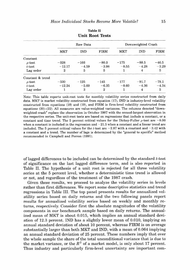
To check this, in Table I1 we employ augmented Dickey and Fuller (1979) p-tests and t-tests, based on regressions of time series on their lagged values and lagged difference terms that account for serial correlation. The number


Table I1 Unit Root Tests

Raw Data Downweighted Crash

MKT IND FIRM MKT IND FIRM

Constant p-test -328 -103 -80.3 -175 -88.5 -46.5 t-test -12.17 -4.59 -3.98 -8.55 -4.28 -3.29 Lag order 2 5 5 1 4 5

Constant & trend p-test -330 -125 -145 -177 -91.7 -79.1 t-test -12.24 -5.60 -6.35 -8.60 -4.36 -4.34 Lag order 1 3 2 1 4 5

Note: This table reports unit-root tests for monthly volatility series constructed from daily data. MKT is market volatility constructed from equation (17), IND is industry-level volatility constructed from equations (18) and (19), and FIRM is firm-level volatility constructed from equations (20)-(22). All measures are value-weighted variances. The columns denoted "downweighted crash" replace the observation in October 1987 with the second-largest observation in the respective series. The unit-root tests are based on regressions that include a constant, or a constant and time trend. The 5 percent critical values for the Dickey-Fuller p-test are -8.00 when a constant is included in the regression and -21.5 when a constant and a linear trend are included. The 5 percent critical values for the t-test are -2.87 with a constant and -3.42 with a constant and a trend. The number of lags is determined by the "general to specific" method recommended in Campbell and Perron (1991).

of lagged differences to be included can be determined by the standard t-test of significance on the last lagged difference term, and is also reported in Table 11. The hypothesis of a unit root is rejected for all three volatility series at the 5 percent level, whether a deterministic time trend is allowed or not, and regardless of the treatment of the 1987 crash.

Given these results, we proceed to analyze the volatility series in levels rather than first differences. We report some descriptive statistics and trend regressions in Table 111. The top panel presents results for annualized volatility series based on daily returns and the two following panels report results for annualized volatility series based on weekly and monthly returns, respectively. Consider first the absolute magnitudes of the volatility components in our benchmark sample based on daily returns. The annualized mean of MKT is about 0.015, which implies an annual standard deviation of 12.3 percent. IND has a slightly lower mean of 0.010, implying an annual standard deviation of about 10 percent, whereas FIRM is on average substantially larger than both MKT and IND, with a mean of 0.064 implying an annual standard deviation of 25 percent. These numbers imply that over the whole sample the share of the total unconditional variance that is due to the market variance, or the R 2 of a market model, is only about 17 percent. Thus industry and particularly firm-level uncertainty are important com-

Daily Mean * 10' Std. dev. * lo2 Std. dev. * 10' detrended Linear trend * lo5 PS-statistic Confidence interval

Weekly Mean * 10' Std. dev. * 10' Std. dev. * 10' detrended Linear trend * lo5 PS-statistic Confidence interval

Monthly mean * 10' Std. dev. * 10' Std. dev. * 10' detrended Linear trend * 10' PS-statistic Confidence interval

Table I11

Descriptive Statistics and Linear Trends

Raw Data

MKT IND FIRM MKT

1.542 1.032 6.436 1.409 3.500 0.663 2.912 1.469 3.488 0.663 2.536 1.463 0.156 0.062 0.965 0.090 0.261 0.086 1.005 0.144

(-0.07, 0.60) (-0.10, 0.27) (0.55, 1.47) (-0.12, 0.41)

1.897 1.218 5.842 1.858 2.522 0.727 2.210 2.158 2.522 0.724 1.923 2.158 0.003 0.053 0.737 -0.017 0.116 0.096 0.410 0.082

(-0.33, 0.56) (-0.13, 0.32) (0.13, 0.69) (-0.36, 0.52)

Downweighted Crash

IND

1.027 0.623 0.619 0.060 0.082

(-0.10, 0.27)

1.218 0.727 0.721 0.053 0.096

(-0.13, 0.32)

FIRM 2 %

6.383 2.446 f 2.013 h

0.939 %

(0.49, 1.42)0.958 ? 3 0

5.842 m 2.210 1.919 0.737 0.410

(0.13, 0.69)

Daily-large firms Mean * lo2 Std. dev. * lo2 Std. dev. * 10' detrended Linear trend * lo5 PS-statistic Confidence interval

Daily-EW Mean * lo2 Std. dev. * 10' Std. dev. * 10' detrended Linear trend * lo5 PS-statistic Confidence interval

1.599 1.090 5.877 1.145 1.086 3.675 0.744 2.671 1.507 0.675 3.464 0.693 2.557 1.498 0.658 0.185 0.087 0.524 0.116 0.085 0.296 0.111 0.590 0.172 0.107

(-0.06, 0.65) (-0.08, 0.31) (0.03, 1.15) (-0.10, 0.45) (-0.09, 0.30)

1.211 1.251 33.903 1.149 1.251 2.619 0.554 23.112 1.718 0.412 2.612 0.554 14.116 1.704 0.554

-0.114 0.022 12.386 -0.145 0.022 -0.076 -0.004 11.231 -0.132 -0.004

(-0.33, 0.17) (-0.15, 0.14) (5.29, 17.17) (-0.38, 0.11) (0.15, 0.14)

5.828 2.210 2.080 0.499 0.055

(-0.02, 1.11)

% 33.903 $ rn 23.112 14.116 2R

p..12.386 z.11.219 (5.30, 17.14)

h

Note: This table reports descriptive statistics and the results of a linear trend regression for monthly volatility measures. MKT is market C$volatility constructed from equation (17),IND is industry-level volatility constructed from equations (18)and (19),and FIRM is firm-level 8 volatility constructed from equations (20)-(22). All measures are value-weighted variances. The top panel uses daily data to construct monthly $ volatilities, the second panel uses weekly data, and the third panel uses monthly data. The panel denoted "large firms" uses only the 2,026firms with the largest capitalization in each month (2,026is the total number of firms at the start of the sample in July 1962).The bottom panel is 8 based on an equal-weighting scheme (denoted EW) as opposed to value weighting for all other results. The columns denoted "downweighted 0

crash" replace the observation in October 1987with the second-largest observation in the respective series. Monthly variances are annualized 2 (multiplied by 12). Means and standard deviations of the annualized variances are multiplied by 100 in this table. The table also reports estimates of a linear trend coefficient (multiplied by lo5),the PS-statistic developed by Yogelsang (1998)to test for the significance of the trend, $ and the implied 90percent confidence interval for the trend coefficient. 2

i2 8.h

",


ponents of the total volatility of an average firm. The means for the data downweighting the crash are, of course, somewhat lower because the crash is replaced by the second largest observation.

All three volatility measures exhibit substantial variation over time. The second row in each panel of Table I11 reports unconditional standard deviations of the variance series. Market and firm volatility are more variable over time than industry volatility, but a large portion of the time-series variation in market volatility is due to the crash in October 1987. Downweight- ing the crash reduces the standard deviation of market volatility by 60 percent. The crash has much smaller effects on industry and firm volatility.

Next we revisit the issue of trends. In Table I1 we rejected the unit root hypothesis for all three volatility series. An alternative hypothesis is the existence of a deterministic linear time trend. Since all volatility series are fairly persistent, standard trend tests are not valid. Hence we employ the procedure suggested in Vogelsang (1998), which is robust to various forms of serial correlation. Vogelsang suggests a Wald-type test based on the following model

where v E {MKT,IND,FIRM},p is an intercept, g is the linear trend coefficient, and p captures the dependence of v on its own first lag. The error term u itself depends on its own first lag through the coefficient a, and on an infinite moving average of the white-noise innovation e through coefficients d(L) = X E d d i L i ,where L is the lag operator. This test is robust to both I(0) and 1(1) errors. Because we rejected a unit root in all volatility series, we use Vogelsang's PS1 test to obtain the best power. Table I11 reports the trend coefficient from a simple OLS regression of volatility on time, the value of the Vogelsang test statistic, and the associated (two-sided) 90 percent confidence interval for the trend coefficient g in equation (23).

The top panel reports results for our benchmark case, the monthly volatility series estimated from daily data. Consider first the raw data. The trend regression for daily data confirms the visual evidence from the plots. MKT and IND have a small positive but insignificant trend coefficient whereas the trend in FIRM is much larger. The PS test statistic for FIRM is positive and significant. Note that the large trend coefficient does not depend on the treatment of the crash.

Our coefficient estimates for data downweighting the crash imply that the firm-level component of variance has more than doubled over the sample, whereas the market and industry components of variance have increased by only about one-third. The total return variance of a randomly selected firm (picking each firm with a probability equal to its market capitalization weight) has also roughly doubled over the sample; our estimates imply that this


increase is almost entirely due to the higher level of idiosyncratic firm-level volatility. Another way to make the same point, again using data that downweight the crash, is to note that, from 1962 to 1997, the share of FIRM volatility in total volatility has increased from 65 percent to 76 percent whereas the shares of MKT and IND have decreased from 20 percent to 14 percent and 15 percent to 10 percent, respectively.

Table I11 also reports standard deviations of the detrended volatility series. A time trend biases the unconditional time-series variation upwards. Because FIRM has the largest trend among the three measures, the standard deviation decreases the most when the data are detrended. The effects of detrending are modest for MKT and IND. Even for detrended data, however, FIRM exhibits the greatest time-series variation once the crash is downweighted.

It is well known that daily stock returns exhibit significant short-run serial correlation. This might affect our volatility series, in particular if the pattern of serial correlation is changing over time (Froot and Perold (1995) document that market-level serial correlation has declined in the postwar period). To check the robustness of the results based on daily returns, we construct volatility series based on weekly and monthly returns for which autocorrelation is much weaker. That is, we change the time interval s in equations (17), (18), and (19) from daily to weekly or monthly, while still keeping the time interval t equal to one month.4 The second and third panels in Table I11 show that the means of MKT and IND increase somewhat for longer horizon returns, confirming the fact that daily index and industry returns are positively autocorrelated. Firm-specific returns, by contrast, are negatively autocorrelated (French and Roll (1986)), so the mean of FIRM decreases when weekly and monthly returns are used. It is interesting to note that the treatment of the crash has little effect on IND and FIRM once weekly or monthly returns are used. This suggests that industry and firm returns took a few days to adjust, but within a week the effect of the crash died out at the industry and firm level.

The return horizon does affect our estimates of volatility trends. Trends are weaker in volatility series based on weekly and monthly data than in the series based on daily data. The point estimate of the trend coefficient for weekly market volatility is even negative (but insignificant) if the crash is downweighted. However, the Vogelsang PS test shows that the trend in FIRM is significantly positive for all three horizons; thus our key result on the upward trend in idiosyncratic volatility is robust to the use of daily, weekly, or monthly returns.

We perform two additional sensitivity checks. As noted above, the number of firms in the data set has more than quadrupled over the sample. Thus many smaller firms are now listed on stock markets. To see how this influ- ences our results, we compute the volatility series using only the 2,047 larg-

When s = t our volatility measures are just squared monthly returns. These are obviously noisy measures of volatility, but they still enable us to estimate long-run means and trends.


est firms (the minimum number of firms in a month of our sample). The results are shown in the Table I11 panel denoted "large firms." In contrast to MKT and IND, which are not much affected by the exclusion of smaller firms, the mean and trend of FIRM are somewhat lower for large firms. The trend of FIRM is still positive but the PS statistic is significant only at the 10 percent level.

The effect of firm size can also be seen in the last panel of Table 111, which reports results for equally weighted series. As in the large-firm case, MKT and IND are not affected much by the weighting scheme. However, the impact on FIRM is enormous. The mean is 5 times larger, the standard deviation is 8 times larger, and the trend coefficient is a startling 12 times larger than for the value-weighted series. The estimated trend implies that firm-level variance is about 30 times higher in 1997 than in 1962 for a typical firm, selected randomly from among all firms with equal probability. This demonstrates the significant effect on volatility of many small firms entering the market over our sample period.

C. Individual Industries

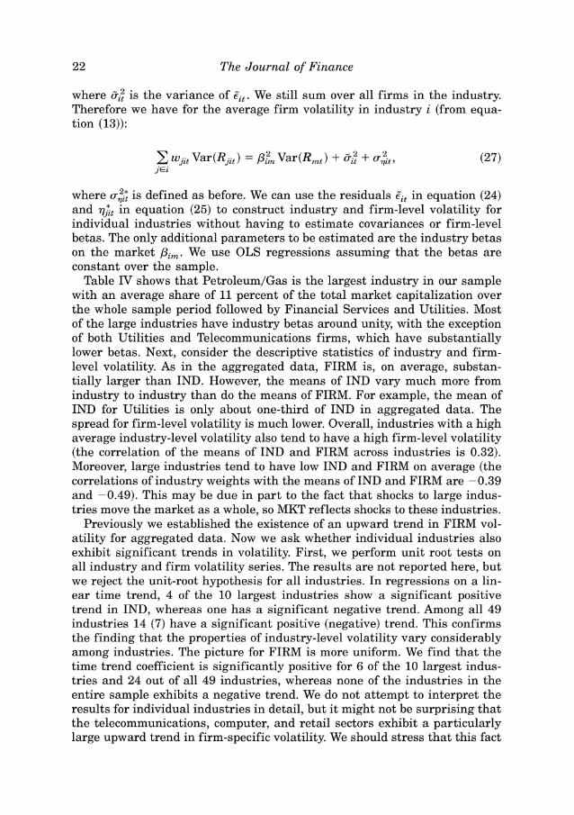
So far we have studied volatilities averaged over industries. Although such aggregated volatility measures contain information about an average industry, there is obviously a great deal of variation across industries. The nature and composition of the industries in our sample differ tremendously, and there is little reason to believe that industry and firm-level volatility in the agricultural sector behave in the same way as volatility in the computer industry. We now examine the 10 largest industries separately, selecting the industries according to their average market capitalization over the entire sample. Table IV lists the individual industries by weight.

Constructing volatility measures for individual industries requires an ad- justment in our estimation procedure. In Section I we showed that the three return components in equation (10) are orthogonal when we average over firms and industries. Once we study individual industries we no longer average over industries. Therefore, we have to alter the return composition in the following way. Consider a decomposition that includes a beta for each industry:

Note that R,, and Sit are by construction orthogonal and therefore the volatility of the industry return is

Table IV Individual Industries R

8 C

IND FIRM m

Industry Weight P Mean s.d. Trend PS-stat Mean s.d. Trend PS-stat 32 .-.

Petroleum/Gas 11.031 0.86 1.013 0.302 0.249 0.334 5.498 0.774 0.583 0.946 '. Fin. Services 7.833 0.97 0.362 0.102 -0.125 -0.158 6.361 0.871 0.224 0.484 3 Utilities 7.446 0.66 0.311 0.097 0.033 0.030 4.032 0.500 0.125 0.228 Consumer Goods 6.117 1.02 0.562 0.122 0.016 0.026 4.590 0.598 -0.006 0.157 3 Telecomm. 5.699 0.70 0.811 0.176 -0.065 -0.067 3.729 0.826 1.555 1.334 $ Computer 4.995 1.06 1.654 0.398 0.070 -0.001 6.123 1.536 2.867 2.311 Retail 4.596 1.09 0.586 0.132 0.049 0.028 7.332 0.919 1.367 1.465 Auto 4.295 1.02 1.115 0.231 0.138 0.117 4.862 0.695 0.754 0.922 3 Pharmaceutical 4.206 1.00 0.792 0.228 0.167 0.133 6.126 0.745 0.780 0.578 Chemical 3.812 1.05 0.517 0.103 0.077 0.064 5.281 0.618 0.448 0.655 m

-Note: This table reports descriptive statistics for industry and firm volatilities in the 10 industries with the largest average market capitaliza- 5 tion. Industry volatility IND is constructed using equation (26), and firm volatility FIRM is constructed using equation (27).All volatilities are m 1

measured monthly, on a value-weighted basis, using daily data. Weight is computed as the ratio of the average market value of firms in an industry to the average total market value of all firms. Beta is computed using a regression of monthly industry excess returns on the monthly excess return of the CRSP value-weighted index. Monthly variances are annualized (multiplied by 12). Means and standard deviations of the g. annualized variances are multiplied by 100 in this table. The table also reports estimates of a linear trend coefficient (multiplied by lo5), and the PS-statistic developed by Vogelsang (1998) to test for the significance of the trend. A bold statistic indicates that a zero trend is outside the 90 percent confidence interval.

2 2 The Journal of Finance

where ei:is the variance of Ci,. We still sum over all firms in the industry. Therefore we have for the average firm volatility in industry i (from equation (13)):

where is defined as before. We can use the residuals Zitin equation (24) and q;, in equation (25) to construct industry and firm-level volatility for individual industries without having to estimate covariances or firm-level betas. The only additional parameters to be estimated are the industry betas on the market pi,. We use OLS regressions assuming that the betas are constant over the sample.

Table IV shows that Petroleum/Gas is the largest industry in our sample with an average share of 11percent of the total market capitalization over the whole sample period followed by Financial Services and Utilities. Most of the large industries have industry betas around unity, with the exception of both Utilities and Telecommunications firms, which have substantially lower betas. Next, consider the descriptive statistics of industry and firm- level volatility. As in the aggregated data, FIRM is, on average, substantially larger than IND. However, the means of IND vary much more from industry to industry than do the means of FIRM. For example, the mean of IND for Utilities is only about one-third of IND in aggregated data. The spread for firm-level volatility is much lower. Overall, industries with a high average industry-level volatility also tend to have a high firm-level volatility (the correlation of the means of IND and FIRM across industries is 0.32). Moreover, large industries tend to have low IND and FIRM on average (the correlations of industry weights with the means of IND and FIRM are -0.39 and -0.49). This may be due in part to the fact that shocks to large industries move the market as a whole, so MKT reflects shocks to these industries.

Previously we established the existence of an upward trend in FIRM volatility for aggregated data. Now we ask whether individual industries also exhibit significant trends in volatility. First, we perform unit root tests on all industry and firm volatility series. The results are not reported here, but we reject the unit-root hypothesis for all industries. In regressions on a linear time trend, 4 of the 10 largest industries show a significant positive trend in IND, whereas one has a significant negative trend. Among all 49 industries 14 (7) have a significant positive (negative) trend. This confirms the finding that the properties of industry-level volatility vary considerably among industries. The picture for FIRM is more uniform. We find that the time trend coefficient is significantly positive for 6 of the 10 largest industries and 24 out of all 49 industries, whereas none of the industries in the entire sample exhibits a negative trend. We do not attempt to interpret the results for individual industries in detail, but it might not be surprising that the telecommunications, computer, and retail sectors exhibit a particularly large upward trend in firm-specific volatility. We should stress that this fact


is not the result of an unusual increase in the number of listed firms in these industries. The time trend in the sample that includes only large firms shows the same large trend in firm-level volatility for these industries.

111. Portfolio Implications of the Increase in Idiosyncratic Volatility

We have shown that aggregate stock market volatility has been quite stable over time, whereas firm-level volatility has trended upwards. An impli- cation of this finding is that there should be a declining trend in the correlations among individual stock returns. Declining correlations allow the volatility of the market portfolio to remain the same even if there is an increase in each individual stock's volatility.

We document the evolution of correlations among individual stocks by cal- culating all pairwise correlations among stocks traded on the NYSE, AMEX, and Nasdaq.5 We use both daily and monthly data. Correlations using daily data are calculated each month, using the previous 12 months of daily ob- servations (or as many months as are available at the beginning of the data set). The number of stocks in the sample at each month ranges from about 1,500 to about 8,000, so the number of pairwise correlations ranges from just over 1 million to 32 million. We calculate an equally weighted average of these correlations. Correlations using monthly data are again calculated each month, but they use the previous 60 months of monthly returns. Somewhat fewer stocks have a complete five-year history than have a one-year history, so the number of stocks in the sample ranges from 1,000 to 4,500, and the number of pairwise correlations from half a million to just over 10 million. Again we calculate an equally weighted average for the month. The results are reported in the top panel of Figure 5.

The figure shows a clear tendency for correlations among individual stock returns to decline over time. Correlations based on five years of monthly data decline from 0.28 in the early 1960s to 0.08 in 1997, and correlations based on one year of daily data decline from 0.12 in the early 1960s to between 0.02 and 0.04 in the 1990s. The former correlations are larger than the latter, both because daily stock returns contain negatively autocorrelated idiosyncratic components, and because correlations are lower in more recent data, which receive greater weight in the daily calculation.

The bottom panel of Figure 5 plots the average R2 statistic for the market model, using the same stocks as the top panel. For each stock, the market model is estimated using five years of monthly or one year of daily data, and using the NYSE/AMEX/Nasdaq composite index as the market index. The resulting R2 statistic is averaged across stocks. The two panels of the figure are almost indistinguishable from one another. This is not surprising; if all

ti We exclude stocks with daily returns exceeding 200 percent, or with zero returns on at least 75 percent of the days in the last 12 months. These filters exclude spurious returns resulting from missing data, and stocks that are traded very infrequently.


P a n e l A: Average c o r r e l a t i o n s a m o n g ind iv idua l s t o c k s

Date

Pane l B: Average R~ s t a t i s t i c s of m a r k e t m o d e l f o r ind iv idua l s t o c k s

Figure 5. Average correlations and Ra statistics of market model for individual stocks. The top panel reports the equally weighted average pairwise correlation across stocks traded on the NYSE, AMEX, and Nasdaq. The solid line is the average correlation over the past 60 months of monthly data, and the dotted line is the average correlation over the past 12 months of daily data. The bottom panel reports the equally weighted average R2 statistic of a market model, estimated using the past 60 months of monthly data (solid line) or the past 12 months of daily data (dotted line). Stocks included in the calculation a t each point in time are required to have a complete return history over the past 60 months (solid line) or 12 months (dotted line).


stocks were identical and had the same correlation p with each other, then the variance of the market portfolio would be p times the variance of any individual stock, and the R2 of the market model would be p. While stocks are not of course identical, this relationship remains a good approximation.

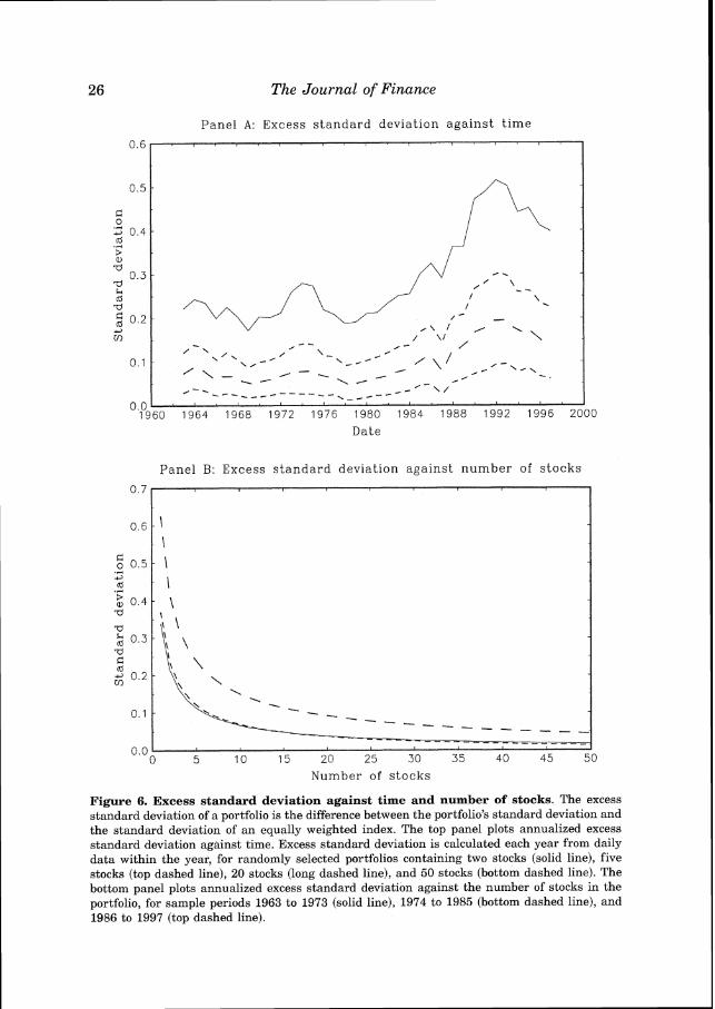
Declining correlations among stocks imply that the benefits of portfolio diversification have increased over time. An investor who holds only one stock bears the full risk of the individual stock, whereas an investor who holds a sufficient number of stocks bears only market risk. As individual stock volatility has increased relative to market volatility, the difference between these risks has increased. We illustrate this point in Figure 6, which shows the excess standard deviations of portfolios containing different numbers of randomly selected stocks-that is, the differences between the standard deviations of such portfolios and the standard deviation of an equally weighted index of all stocks.

The top panel of Figure 6 shows the annualized excess standard deviation each year, calculated from daily data during the year, of equally weighted portfolios containing 2, 5, 20, and 50 stocks over the standard deviation of an equally weighted index. We use the same universe of stocks as for Fig- ure 5, randomly grouping them into portfolios without replacement and cal- culating a simple average of portfolio standard deviations across portfolios. The figure shows a modest increase in the excess standard deviation of a typical 50-stock portfolio, but a much more dramatic increase in the excess standard deviation of a typical 2-stock portfolio, from about 25 percent in the early 1960s to a peak of 50 percent in the early 1990s.

The bottom panel of Figure 6 makes the same point in a different way. The full sample is broken into three subsamples, 1963 to 1973, 1974 to 1985, and 1986 to 1997. For each subsample the average annualized excess standard deviation of an equally weighted portfolio is plotted against the number of stocks in the portfolio. Diagrams of this sort are often used in textbooks to illustrate the benefits of portfolio diversification (see, e.g., Bodie, Kane, and Marcus (1999), p. 203). A conventional rule of thumb, supported by the results of Bloomfield, Leftwich, and Long (1977), is that a portfolio of 20 stocks attains a large fraction of the total benefits of diversification. Figure 6 shows, however, that the increase in idiosyncratic risk has increased the number of stocks needed to reduce excess standard deviation to any given level. In the first two subsamples a portfolio of 20 stocks reduced annualized excess standard deviation to about five percent, but in the 1986 to 1997 subsample, this level of excess standard deviation required almost 50 stock^.^ To put the result another way, the increase in idiosyncratic volatility over time has increased the number of randomly selected stocks needed to achieve relatively complete portfolio diversification.

Bloomfield et al. (1977) report lower standard deviations for small equally weighted portfolios. The difference is probably due to their 1965 to 1970 sample period and their use of stocks with continuous price histories. However our results for 1963 to 1973 confirm their conclusion that substantial diversification could be achieved in the late 1960s with portfolios of fewer than 20 stocks.


Date

Pane l B: Excess s t a n d a r d deviat ion aga ins t n u m b e r of s tocks

Number of s tocks

Figure 6. Excess standard deviation against time and number of stocks. The excess standard deviation of a portfolio is the difference between the portfolio's standard deviation and the standard deviation of an equally weighted index. The top panel plots annualized excess standard deviation against time. Excess standard deviation is calculated each year from daily data within the year, for randomly selected portfolios containing two stocks (solid line), five stocks (top dashed line), 20 stocks (long dashed line), and 50 stocks (bottom dashed line). The bottom panel plots annualized excess standard deviation against the number of stocks in the portfolio, for sample periods 1963 to 1973 (solid line), 1974 to 1985 (bottom dashed line), and 1986 to 1997 (top dashed line).


TableV

Correlation Structure

With Trend Detrended

MKT IND FIRM MKT IND FIRM

Note: This table reports the contemporaneous correlation structure of monthly volatility measures constructed from daily data, downweighting the crash of October 1987 by replacing it with the second largest observation in the time series. MKT is market volatility constructed from equation (17), IND is industry- level volatility constructed from equations (18) and (19), and FIRM is firm-level volatility constructed from equations (20)-(22). All measures are value- weighted variances. The left panel reports correlations of the series themselves, the right panel reports correlations of the detrended series.

IV. Short-Run Volatility Dynamics

A. Covariation and Lead-Lag Relationships

We have emphasized trends in volatility over time. But i t is clear from Figures 2 to 4 that there are many short-run movements around these trends, and these movements tend to be correlated across our three volatility measures. We examine this aspect of the data in Table V, both for raw and detrended data. Here and in all subsequent tables we downweight the crash of 1987 in the manner previously described. Table V shows contemporaneous correlations of volatility measures around 0.7, and even slightly higher for detrended data.

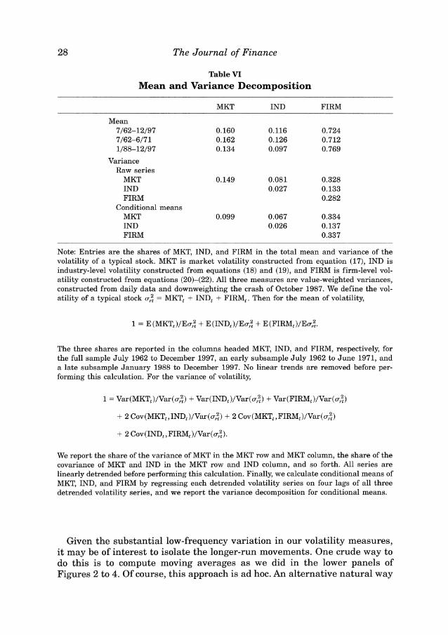
Table VI asks how important the three volatility components are relative to the total volatility of an average firm. First, consider the mean. Over the whole sample, market volatility accounts for about 16 percent of the unconditional mean of total volatility, whereas IND accounts for 12 percent. How- ever, by far the largest portion of total volatility is firm-level volatility, with about 72 percent. Consistent with the observation of trends in the three series, the share of firm-level volatility has increased from 71 percent in the first nine years of the sample to 77 percent in the last nine years.

A variance decomposition shows that most of the time-series variation in total volatility is due to variation in MKT and FIRM. Industry volatility is more stable over time. The two largest components are FIRM variance and the covariation of MKT and FIRM; together they account for about 60 percent of the total time-series variation in volatility. The market component by itself is much less important, only 15 percent of the total variation in volatility. Relative to its mean, however, MKT shows the greatest time-series variation.


TableVI Mean and Variance Decomposition

MKT IND FIRM

Mean 7/62-12/97 7/62-6/7 1 1/88-12/97

Variance Raw series

MKT IND FIRM

Conditional means MKT IND FIRM

Note: Entries are the shares of MKT, IND, and FIRM in the total mean and variance of the volatility of a typical stock. MKT is market volatility constructed from equation (17), IND is industry-level volatility constructed from equations (18) and (19), and FIRM is firm-level volatility constructed from equations (20)-(22). All three measures are value-weighted variances, constructed from daily data and downweighting the crash of October 1987. We define the volatility of a typical stock a; = MKT, + IND, + FIRM,. Then for the mean of volatility,

The three shares are reported in the columns headed MKT, IND, and FIRM, respectively, for the full sample July 1962 to December 1997, an early subsample July 1962 to June 1971, and a late subsample January 1988 to December 1997. No linear trends are removed before performing this calculation. For the variance of volatility,

We report the share of the variance of MKT in the MKT row and MKT column, the share of the covariance of MKT and IND in the MKT row and IND column, and so forth. All series are linearly detrended before performing this calculation. Finally, we calculate conditional means of MKT, IND, and FIRM by regressing each detrended volatility series on four lags of all three detrended volatility series, and we report the variance decomposition for conditional means.

Given the substantial low-frequency variation in our volatility measures, it may be of interest to isolate the longer-run movements. One crude way to do this is to compute moving averages as we did in the lower panels of Figures 2 to 4. Of course, this approach is ad hoc. An alternative natural way

Have Individual Stocks Become More Volatile? 29

to smooth the series is to decompose each volatility time series into an expected and an unexpected part:

where v E {MKT,IND,FIRM). We compute the conditional expectation of each volatility series by regressing it on its own lags and on the lags of the other series. Based on the significance of individual lags, we choose a lag length of four when forming the conditional expectations.

At the bottom of Table VI we report a variance decomposition for the conditional expectations of the volatility series. This puts even more weight on the terms involving FIRM; about 80 percent of the total variation is due to variance and covariance terms of FIRM. The contribution of MKT is below 10 percent. The industry-level terms for conditional expectations are more or less unchanged compared to the raw data.

One issue that arises in interpreting these results is whether the common variation in MKT, IND, and FIRM might be explained by cross-sectional variation in betas. In equation (15), we showed that movements in MKT might produce variation in IND if betas differ across industries and the volatility of industries' CAPM residuals is independent of MKT. Under this hypothesis, the coefficient in a regression of IND on MKT would equal the cross-sectional variance of betas across industries. Empirically, the regression coefficient is 0.27 in our full sample whereas a direct estimate of cross- sectional variance of industry betas is only 0.03; this calculation suggests that cross-sectional variation in betas cannot explain more than a small fraction of the common movement in MKT and IND. A similar calculation based on equation (16) gives the same result for covariation between FIRM and the other two volatility measures. In our full sample, a regression of FIRM on MKT and IND gives coefficients of 0.72 and 1.40, respectively, much too large to be explained by plausible cross-sectional variation in firms' beta coefficients.

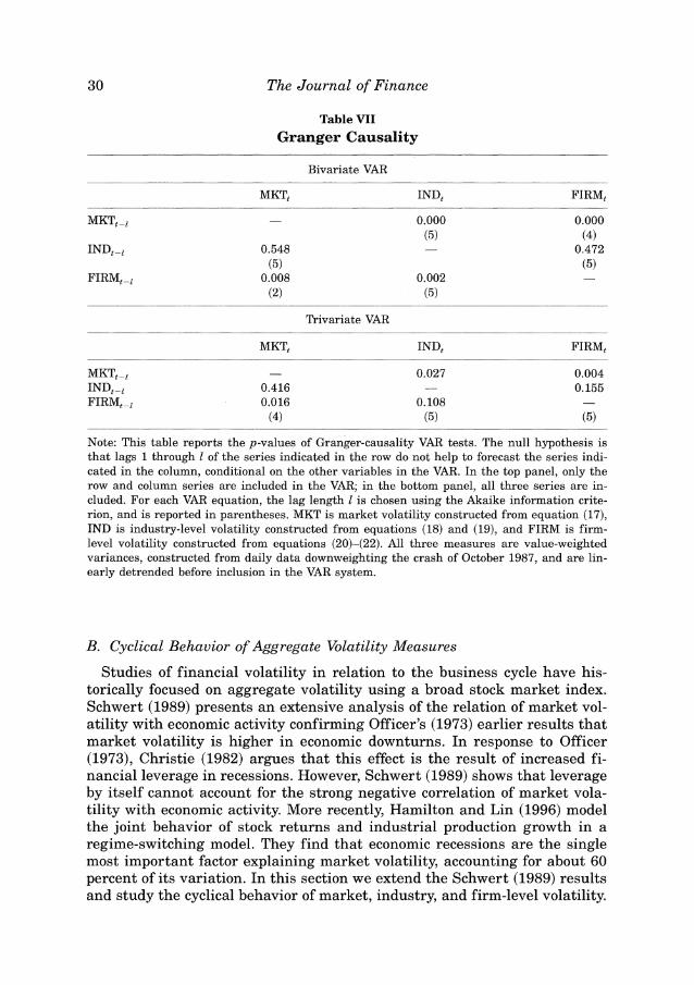
As a final exercise in this section, we ask whether the volatility measures help to forecast each other. Table VII investigates this question using Granger- causality tests. The top panel reports p-values for bivariate VARs and the bottom panel uses trivariate VARs including all three series. The data are detrended and downweight the crash. The VAR lag length was chosen using the Akaike information criterion. In bivariate VARs, MKT appears to Granger- cause both IND and FIRM at very high significance levels. IND does not help to predict MKT or FIRM, but FIRM helps significantly to forecast MKT and IND. Much of the causality survives in trivariate systems. MKT Granger- causes IND and FIRM (although at lower significance levels than in the bivariate case). FIRM Granger-causes MKT but the effect on IND is now insignificant. IND fails to Granger-cause the other series as in the bivariate case. Overall, market volatility appears to lead the other volatility mea-sures, whereas industry volatility tends to lag. Firm-level volatility helps to predict market volatility as well as the other way round.


Table VII Granger Causality

Bivariate VAR

MKT, IND, FIRM,

Trivariate VAR

MKT, IND, FIRM,

MKTt-, - 0.027 0.004 IND,-l 0.416 - 0.155 FIRMt-, 0.016 0.108 -

(4) (5) (5)

Note: This table reports the p-values of Granger-causality VAR tests. The null hypothesis is that lags 1through I of the series indicated in the row do not help to forecast the series indicated in the column, conditional on the other variables in the VAR. In the top panel, only the row and column series are included in the VAR; in the bottom panel, all three series are included. For each VAR equation, the lag length 1 is chosen using the Akaike information criterion, and is reported in parentheses. MKT is market volatility constructed from equation (17), IND is industry-level volatility constructed from equations (18) and (19), and FIRM is firm- level volatility constructed from equations (20)-(22). All three measures are value-weighted variances, constructed from daily data downweighting the crash of October 1987, and are linearly detrended before inclusion in the VAR system.

B. Cyclical Behavior of Aggregate Volatility Measures

Studies of financial volatility in relation to the business cycle have his- torically focused on aggregate volatility using a broad stock market index. Schwert (1989) presents an extensive analysis of the relation of market volatility with economic activity confirming Officer's (1973) earlier results that market volatility is higher in economic downturns. In response to Officer (1973), Christie (1982) argues that this effect is the result of increased financial leverage in recessions. However, Schwert (1989) shows that leverage by itself cannot account for the strong negative correlation of market volatility with economic activity. More recently, Hamilton and Lin (1996) model the joint behavior of stock returns and industrial production growth in a regime-switching model. They find that economic recessions are the single most important factor explaining market volatility, accounting for about 60 percent of its variation. In this section we extend the Schwert (1989) results and study the cyclical behavior of market, industry, and firm-level volatility.

Have Individual Stocks Become More Volatile? 3 1

Figures 2 to 4 suggest that all three volatility components tend to be higher in NBER-dated recessions (shaded in gray). We now characterize this relation more rigorously.

We start by reporting simple correlations of the volatility series with NBER business cycle dates in the top panel of Table VIII. The table reports correlations of the volatility series at various leads and lags with a variable that is set to one in NBER-dated expansions and zero in recessions. Hence a negative correlation implies that volatility tends to be higher in recessions. In addition to correlations for the raw series we also include results for conditional expectations and innovations of volatility (all series are detrended and downweight the crash).

Consider first the raw series. All lead and lag correlations up to a year are negative; hence stock market volatility at the market, industry, and firm level is higher in economic contractions. All three raw series have a strongly negative contemporaneous correlation between -0.420 for MKT and -0.508 for FIRM. The correlation is decreasing in absolute value when volatility is lagged or led (we highlight the most negative correlation in each column in bold). Among the three volatility measures, FIRM tends to have the most negative correlation with NBER dates.

The pattern for conditional expectations is more or less the same as for the raw data. The values tend to be slightly more negative than for the raw data, which is not surprising as the conditional expectations are less noisy. The innovations of volatility are also negatively correlated with NBER dates. But in contrast to the raw data and conditional expectations, the correlations peak (in absolute value) when innovations lead the NBER dates by three months. This pattern holds for all three volatility measures. These results are consistent with Whitelaw (1994), who analyzes the properties of conditional expectations and innovations of market volatility in more detail.

These results provide strong evidence that market, industry, and firm- level volatility are all higher in economic downturns. But how big are the magnitudes? For raw data, the level of market variance is about three times as high in NBER-dated recessions as in expansions. Although this ratio is surprisingly high, Schwert (1989) shows that it is even higher if the Great Depression is included in the sample. Industry-level and firm-level variances roughly double in recessions. Recessions have a somewhat smaller effect on the predictable component of volatility; for conditional expectations, MKT is about 1.9 times higher in recessions than in booms, IND about 1.6 times and FIRM about 1.5 times.

Although the NBER dates provide a benchmark case, some useful information is probably lost in the binary NBER classification scheme. Therefore, we next study the cyclical behavior of volatility using GDP data. GDP is measured on a quarterly frequency; hence we construct new volatility series on that frequency. We use daily returns within each quarter as before. The quarterly series behave very much like the monthly ones. The pattern of correlations of volatility with GDP growth, in the bottom panel of Table VIII, is almost identical to the pattern of correlations with NBER dates. All vol-

TableVIII Cyclical Behavior

Correlation with NBER Dates %3

Volatility Lead MKT IND FIRM

s-R2

(Months) Ut Et-1% <t Ut Et-1% 5t Ut Et- Iut 5t (D


atility series are negatively correlated with GDP growth up to a lead and lag of about one year. The absolute values of the correlations are somewhat lower than before; this is not surprising given the noisiness of GDP data. As before, innovations in volatility show the highest correlation (in absolute value) leading GDP growth by one quarter.

This countercyclical behavior of all volatility measures has important implications for diversification of risk at different stages of the business cycle. Because market volatility is substantially higher in recessions, even a well- diversified portfolio is exposed to more volatility when the economy turns down. The increase in volatility is stronger for an undiversified portfolio, because industry and firm-level volatility also increase in economic downturns. Thus diversification is more important, and requires more individual stock holdings to achieve, when the economy turns down.

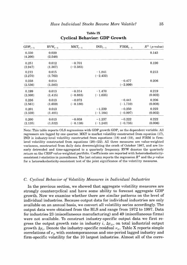
After establishing that all three volatility measures move countercyclically, we now ask whether they have any power to forecast GDP growth. In Table IX we present the results of OLS regressions with GDP growth as a dependent variable. As regressors, we use lagged GDP growth and the lagged return on the value-weighted CRSP index as well as combinations of lagged volatility series. All t-statistics are Newey-West corrected with the optimal lag length chosen according to Newey and West (1994). The volatility series are detrended and downweight the crash. Regressing GDP growth on its own lag and the lagged CRSP index return yields an R2 of 14 percent. Both variables are individually significant. Next, we add each of the lagged volatility measures in turn. Each is individually significant and the R2 increases to around 20 percent. Interestingly, each volatility variable drives out the return of the CRSP value-weighted portfolio, whereas lagged GDP growth remains significant.

Next, we include pairs of volatility variables as regressors. Because all three series are positively correlated, it is not surprising that the individual significance levels are lower when more than one volatility series is included. Although none of them is individually significant, they are strongly jointly significant. The p-values for F-tests that all coefficients of the volatility variables are zero are between 0.2 percent and 0.8 percent. Further- more, the R2s increase to up to 22.2 percent when IND and FIRM are included in the regression. The results are similar when all three volatility variables are included. None of them is individually significant but the joint significance level is 0.6 percent. There is no conclusive evidence indicating which of the three volatility measures has the most forecasting power, but the t-values of IND are slightly higher (in absolute value) than those of MKT and FIRM and the R2 is higher once IND is included in the regression.7

We have also checked whether GDP growth has any ability to forecast volatility, but found no significant results.


Table IX Cyclical Behavior: GDP Growth

GDPt- RV%-I MKTt-, IND,-l FIRMt-, R2 (p-value)

0.330 (4.200)

0.020 (2.548)

0.143

0.251 (2.947)

0.211 (2.270)

0.238 (2.536)

0.012 (1.367)

0.015 (1.762)

0.014 (1.583)

-0.701 (-2.383)

-1.841 (-2.432)

-0.477 (-2.999)

0.190

0.213

0.206

Note: This table reports OLS regressions with GDP growth GDP, as the dependent variable. All regressors are lagged by one quarter. MKT is market volatility constructed from equation (17), IND is industry-level volatility constructed from equations (18) and (19), and FIRM is firm- level volatility constructed from equations (20)-(22). All three measures are value-weighted variances, constructed from daily data downweighting the crash of October 1987, and are linearly detrended and time-aggregated to a quarterly frequency. R W denotes the quarterly return on the CRSP value-weighted portfolio. Coefficients are reported with heteroskedasticity- consistent t-statistics in parentheses. The last column reports the regression R 2 and the p-value for a heteroskedasticity-consistent test of the joint significance of the volatility measures.

C. Cyclical Behavior of Volatility Measures in Individual Industries

In the previous section, we showed that aggregate volatility measures are strongly countercyclical and have some ability to forecast aggregate GDP growth. Now we examine whether there are similar patterns on the level of individual industries. Because output data for individual industries are only available on an annual basis, we convert all volatility series accordingly. The output data were obtained from the BLS and range from 1972 to 1997. Data for industries 23 (miscellaneous manufacturing) and 49 (miscellaneous firms) were not available. To construct industry-specific output data we first re- gress the output growth rate in industry i, Ay,,, on total industrial output growth Ay,. Denote the industry-specific residual v,,. Table X reports simple correlations of vi,with contemporaneous and one-period lagged industry and firm-specific volatility for the 10 largest industries. Almost all of the corre-

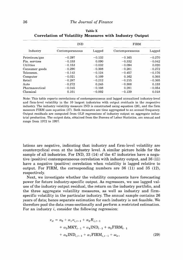
3 6 The Journal of Finance

Table X

Correlation of Volatility Measures with Industry Output

IND FIRM

Industry Contemporaneous Lagged Contemporaneous Lagged

Petroleum/gas Fin. services Utilities Consumer goods Telecomm. Computer Retail Auto Pharmaceutical Chemical

Note: This table reports correlations of contemporaneous and lagged annualized industry-level and firm-level volatility in the 10 largest industries with output residuals in the respective industry. The industry volatility measure IND is constructed using equation (26), and the firm measure FIRM uses equation (27). Both measures are time aggregated to an annual frequency. Output residuals are computed from OLS regressions of industry output on aggregate industrial production. The output data, obtained from the Bureau of Labor Statistics, are annual and range from 1972 to 1997.

lations are negative, indicating that industry and firm-level volatility are countercyclical even at the industry level. A similar picture holds for the sample of all industries. For IND, 33 (14) of the 47 industries have a negative (positive) contemporaneous correlation with industry output, and 36 (11) have a negative (positive) correlation when volatility is lagged relative to output. For FIRM, the corresponding numbers are 36 (11) and 35 (12), respectively.

Next, we investigate whether the volatility components have forecasting power for future industry-specific output. As regressors, we use lagged values of the industry output residual, the return on the industry portfolio, and the three aggregate volatility measures, as well as industry and firm- specific volatility in the particular industry. The annual sample contains 26 years of data; hence separate estimation for each industry is not feasible. We therefore pool the data cross-sectionally and perform a restricted estimation. For an industry i, consider the following regression:


where Ri,,-, is the return on the industry portfolio, and INDi,,-, and FIRM,,,-,are industry and firm-level volatilities computed from the decomposition (24) and (25). We stack all industries into a single system and estimate the model imposing the restriction that the coefficients are identical across all industries. Using Newey-West corrected standard errors, we find that the only significant variable is firm-specific volatility in the industry. The point estimate of a, is -0.158 with a t-statistic of -2.345. However, the R~ of the regression is only 1.2 percent, indicating that industry-specific output residuals are very noisy.

The forecasting power increases somewhat if we use raw industry output data instead of residuals. Although the above specification constructs pure industry effects net of aggregate output, it cannot be used to forecast industry output because aggregate output in period t is not known at time t - 1. We therefore use the following pooled regression:

As for the industry output residuals, the coefficient on industry-level FIRM is significantly negative. The point estimate is a, = -0.190 with a t-statistic of -2.559. The only other significant variable is lagged industry output growth: a , = 0.216 with a t-statistic of 3.996. The R~ is 6.3 percent. Although this forecasting power is still modest, it is interesting to note that firm-level volatility in a given industry is significantly negatively related to future output growth in that industry.

V. What Might Explain Increasing Idiosyncratic Volatility?

We have documented a dramatic increase over the past three decades in the idiosyncratic volatility of stock returns. It is natural to ask what forces might be responsible for this change in stock market behavior. Here we briefly discuss some possibilities, leaving a detailed investigation for future research.

It is helpful at the outset to make a clear distinction between shocks to expected future cash flows, discounted at a constant rate, and shocks to discount rates. Any model that rules out explosive "rational bubbles" in stock prices implies that stock returns must be driven by some combination of these shocks. Thus an increase in volatility can only result from an increase in the variance of cash-flow shocks, an increase in the variance of discount- rate shocks, or an increase in the covariance between the two types of shocks. Campbell (1991) provides an approximate loglinear accounting framework that can be used to break stock market volatility into these components, but the general point does not depend on the use of this approximation.


The strict random-walk model of stock prices implies that stock returns are unforecastable; equivalently, discount rates are constant, so that stock returns are driven entirely by expected future cash flows. Even modest pre- dictability of stock returns, however, can generate important volatility be- yond that arising from shocks to cash flows. Campbell (1991) argues that the bulk of aggregate market volatility arises from changing discount rates. Vuolteenaho (1999) applies a similar methodology to individual stock returns and estimates that shocks to individual firms' cash flow have a variance about twice that of shocks to individual firms' discount rates. The cash flow shocks are less highly correlated across firms than are the discount rate shocks, however, so cash flow news plays a smaller role at the aggregate level.

There is some evidence that the volatility of aggregate output fluctuations has diminished since the early 1980s. McConnell and Perez Quiros (1999) document this fact and attribute it to reduced volatility of production and inventory investment in the durable goods sector. However this phenomenon does not explain the trends reported in this paper because the increased importance of idiosyncratic stock market risk is due to an increase in idiosyncratic volatility, not a reduction in aggregate stock market volatility.

There are several possible reasons why the variance of idiosyncratic shocks to cash flows might have increased over the past several decades. In corporate governance, there has been a strong tendency to break up conglomer- ates and replace them with more focused companies specializing in a single industry or economic activity. This can be understood as a shift towards reliance on external as opposed to internal capital markets (Gertner, Scharf- stein, and Stein (1994), Stein (1997)). I t implies that firms are now separately listed, and their idiosyncratic risks separately measured, whereas previously they might have traded as a single conglomerate that was itself a diversified portfolio of activities.

A related trend is that companies have begun to issue stock earlier in their life cycles, often at a stage where profitability is not yet clearly established and there is considerable uncertainty about long-run prospects. This trend probably has only a small effect on our value-weighted results, but it is surely important for the dramatic increase in equally weighted idiosyncratic volatility reported in the bottom panel of Table 111, and for the equally weighted correlation results reported in Section 111.

Changes in executive compensation may also play a role in these develop- ments. Executives who are compensated through stock options have incen- tives to increase the risks of their firms' activities. Cohen, Hall, and Viceira (2000) study a panel of large firms and find that this effect is statistically detectable, albeit small in magnitude.

Morck, Yeung, and Yu (2000) provide further suggestive evidence for the importance of these factors. They study variation across countries in the explanatory power of the market model, using each country's own stock index as the market index. They find that the market model has much greater explanatory power in less-developed markets with weak legal protection for outside investors. They argue that such markets rely more heavily on inter-


nal finance, with cross-holdings and cross-subsidization that prevent individual firms' stock prices from reflecting information about the values of their core operations.

Leverage is another factor that can affect the volatility of cash flows to equity investors (Black (1976), Christie (1981)). When leverage increases, stockholders bear a greater share of the total cash-flow risk of the firm, and the volatility of the stock return increases accordingly. Leverage certainly accounts for some of the extreme volatility in the Great Depression, illus- trated in Figure 1. Unfortunately recent trends in leverage do not help to explain our findings; the bull market of the 1990s has decreased U.S. corporate leverage, measured in the theoretically appropriate manner using market values, even as idiosyncratic volatility has increased.

It is tempting to argue that idiosyncratic volatility might have increased not just because idiosyncratic cash flows are now separately traded, but also because information about these cash flows is now disseminated far more rapidly. Information technology has certainly helped to make firm-specific information available on a more timely basis. It is important to note, however, that within a framework of constant discount rates, improved information about future cash flows actually decreases volatility rather than increasing it. The reason was explained by West (1988), following Shiller (1981) and LeRoy and Porter (1981). Improved information about future cash flows increases the volatility of the stock-price level, but it reduces the volatility of the stock return because news arrives earlier, at a time when the cash flows in question are more heavily discounted.

Financial innovation-particularly the opening of new derivatives markets- may also have affected the availability of information about future cash flows. As argued by Ross (1976) and John (1984), options can complete an otherwise incomplete market and can have a significant impact on the price behavior of the underlying securities. Theoretically, the direction of this effect is ambiguous. The normal presumption is that derivatives markets increase information and hence reduce volatility (Grossman (1989)); but Stein (1987) points out that it is possible for new derivatives markets to change the pattern of trading by informed speculators in such a way that the information content of prices is reduced, and volatility is increased. Empirically, however, there is little evidence that this perverse effect is important. Kumar, Sarin, and Shastri (1998) and earlier studies cited there, notably Conrad (1989) and Skinner (1989), report that optioned stocks, on average, experi- ence a statistically significant decline in volatility relative to the market as a whole. Thus there is little scientific support for the popular belief that the proliferation of derivative instruments increases volatility.

Shocks to investors' discount rates can also affect idiosyncratic volatility. Within the framework of the CAPM, for example, changes in betas can move discount rates and, hence, prices. If betas are now more volatile, this would explain increased firm-level volatility. Braun, Nelson, and Sunier (1995) find little evidence that beta shocks are important for volatility of industry and size portfolios, but Cho and Engle (1999) obtain more encouraging results for a sample of nine large individual stocks.


An alternative paradigm emphasizes that discount rates are determined by the interactions of heterogeneous groups of investors. One of the most noticeable recent changes in the stock market is the increased share of institutional ownership, particularly in large stocks. Institutional investors-notably pen-sion funds and mutual funds-form a small, relatively homogeneous group whose sentiment may be influenced by a few common factors. This suggests that shocks to institutional sentiment might be important in explaining the increased idiosyncratic volatility of stock returns. Malkiel and Xu (1999) explore this effect in a sample of S&P 500 stocks and find that the proportion of institutional ownership is correlated with volatility. This could of course be due to reverse causality, because institutions prefer more liquid, heavily traded stocks, which may tend to be more volatile (Gompers and Metrick (1999)). However Malkiel and Xu (1999) show that institutional ownership helps to forecast volatility in industry portfolios formed from S&P500 stocks. Day trading by small individual investors may also be an influence on the idiosyncratic volatility of some stocks, particularly at the end of our sample period.

VI. Concluding Comments

In this paper we have characterized the behavior of stock market volatility- not only at the level of the market as a whole, but also at the industry and idiosyncratic firm levels. Our approach has two characteristic features.

First, we have used daily data to construct realized monthly volatility, which we then treat as observable. This allows us to use standard econo- metric methods to describe the time-series variation of realized volatility, rather than the more advanced methods that are necessary when volatility is treated as an unobserved latent variable. Second, we define volatility components in such a way that we can construct the total volatility of a typical firm by adding up components, without regard to covariance terms, and yet we avoid the estimation of industry or firm-level beta coefficients. Both these features can be modified in future research, but they help enormously in the initial exploration of the data.

Our main results are as follows. First, in our 1962 to 1997 sample period, there is strong evidence of a positive deterministic trend in idiosyncratic firm-level volatility. This trend is not due merely to an increase in the number of publicly traded companies or to changes in the serial correlation of daily data. There is no similar trend in industry or market volatility.

Second, the trend increase in idiosyncratic volatility relative to market volatility implies that the correlations among individual stock returns have declined over the past few decades. The R~ of the market model for a typical stock has also declined, while the number of stocks needed to obtain any given amount of portfolio diversification has increased.

Third, firm-level volatility both accounts for the greatest share of total firm volatility, on average, and for the greatest share of the movements over time in total firm volatility. Relative to its mean, however, market volatility displays the greatest variation over time and it tends to lead the other components of volatility.


Fourth, all the components of volatility are countercyclical and tend to lead variations in GDP. The volatility measures help to forecast GDP growth and greatly diminish the significance of stock index returns in forecasting GDP.

Finally, we obtain broadly similar results when we disaggregate to the level of individual industries, using estimates of industry betas on the aggregate market but still avoiding the estimation of firm-level betas.

Like most other papers on volatility, this paper has presented a statistical description rather than a structural economic model. A fascinating area for future research will be to explain the behavior of our disaggregated volatility measures, and particularly the observed upward trend in idiosyncratic volatility. We have speculated that the trend may result in part from changes in corporate governance and in part from the institutionalization of equity ownership, but at this stage any such explanation can only be highly tentative.

REFERENCES

Andersen, Torben G., Tim Bollerslev, Francis X. Diebold, and Paul Labys, 1999, The distribution of stock return volatility, Working paper, Northwestern University, Duke University, and University of Pennsylvania.

Bekaert, Geert, and Campbell R. Harvey, 1997, Emerging equity market volatility, Journal of Financial Economics 43, 29-77.

Bernard, Andrew B., and Douglas G. Steigerwald, 1993, Cleansing recessions: Evidence from stock prices, Working paper, MIT and University of California at Santa Barbara.

Black, Fischer, 1976, Studies of stock price volatility changes, Proceedings of the 1976 Meetings of the Business and Economic Statistics Section, 177-181, American Statistical Association.

Bloomfield, Ted, Richard Leftwich, and John B. Long, Jr., 1977, Portfolio strategies and per- formance, Journal of Financial Economics 5, 201-218.

Bodie, Zvi, Alex Kane, and Alan J. Marcus, 1999, Investments, fourth edition (Irwin McGraw- Hill, New York).

Bollerslev, Tim, Ray Chou, and Kenneth Kroner, 1992, ARCH modeling in finance: A review of the theory and empirical evidence, Journal of Econometrics 52, 5-59.

Brainard, S. Lael, and David M. Cutler, 1993, Sectoral shifts and cyclical unemployment re- considered, Quarterly Journal of Economics 108, 219-243.

Braun, Phillip A., Daniel B. Nelson, and Alain M. Sunier, 1995, Good news, bad news, volatility, and beta, Journal of Finance 50, 1575-1603.

Caballero, Ricardo J., and Mohammed Hammour, 1994, The cleansing effect of recessions, Amer-ican Economic Review 84, 1350-1368.

Campbell, John Y., 1991, A variance decomposition for stock returns, Economic Journal 101, 157-179.

Campbell, John Y., Sangjoon Kim, and Martin Lettau, 1994, Dispersion and volatility in stock returns: An empirical investigation, Working paper, Princeton University.

Campbell, John Y., and Martin Lettau, 1999, Dispersion and volatility in stock returns: An empirical investigation, NBER Working paper 7144.

Campbell, John Y., Andrew W. Lo, and A. Craig MacKinlay, 1997, The Econometrics of Financial Markets (Princeton University Press, Princeton, NJ).

Campbell, John Y., and Pierre Perron, 1991, Pitfalls and opportunities: What macroeconomists should know about unit roots, NBER Macroeconomics Annual 6, 141-201.

Cho, Young-Hye, and Robert F. Engle, 1999, Time-varying betas and asymmetric effects of news: Empirical analysis of blue chip stocks, NBER Working paper 7330.

Christie, Andrew, 1982, The stochastic behavior of common stock variances: Value, leverage, and interest rate effects, Journal of Financial Economics 10, 407-432.

Cohen, Randolph B., Brian J. Hall, and Luis M. Viceira, 2000, Do executive stock options en- courage risk-taking?, Working paper, Harvard Business School.


Conrad, Jennifer, 1989, The price effect of option introduction, Journal of Finance 44, 487-498. Dickey, David, and Wayne Fuller, 1979, Distribution of the estimators for autoregressive time

series with a unit root, Journal of the American Statistical Association 74, 427-431. Duffee, Gregory R., 1995, Stock returns and volatility: A firm-level analysis, Journal of Finan-

cial Economics 37, 399-420. Eden, Benjamin, and Boyan Jovanovic, 1994, Asymmetric information and the excess volatility

of stock prices, Economic Inquiry 32, 228-235. Engle, Robert F., and G.G.J. Lee, 1993, Long run volatility forecasting for individual stocks in

a one factor model, Working paper, University of California at San Diego. Fama, Eugene F., and Kenneth R. French, 1997, Industry costs of equity, Journal of Financial

Economics 43, 153-194. Foster, Dean P., and Daniel B. Nelson, 1996, Continuous record asymptotics for rolling sample

variance estimators, Econometrica 64, 139-174. French, Kenneth, and Richard Roll, 1986, Stock return variances: The arrival of information

and the reaction of traders, Journal of Financial Economics 19, 3-30. French, Kenneth, G. William Schwert, and Robert Stambaugh, 1987, Expected stock returns

and volatility, Journal of Financial Economics 19, 3-30. Froot, Kenneth, and Andre Perold, 1995, New trading practices and short-run market effi-

ciency, Journal of Futures Markets 15, 731-765. Gertner, Robert H., David S. Scharfstein, and Jeremy C. Stein, 1994, Internal versus external

capital markets, Quarterly Journal of Economics 109, 1211-1230. Ghysels, Eric, Andrew Harvey, and E. Renault, 1996, Stochastic volatility, in G.S. Maddala, ed.:

Handbook of Statistics, Vol. 14 (North-Holland, Amsterdam). Gompers, Paul A,, and Andrew Metrick, 1999, Institutional investors and equity prices, Work-

ing paper, Harvard University. Grossman, Sanford, 1989, An analysis of the implications for stock and futures price volatility

of program trading and dynamic hedging strategies, in S. Grossman, ed.: The Informa- tional Role of Praces, Wicksell Lectures (MIT Press, Cambridge, MA).

Hamilton, James D., and Gang Lin, 1996, Stock market volatility and the business cycle, Jour-nal of Applied Econometrics 11,573-593.

Hentschel, Ludger, 1995, All in the family: Nesting symmetric and asymmetric GARCH models, Journal of Financial Economics 39, 71-104.

Heston, Steven L., and K. Geert Rouwenhorst, 1994, Does industrial structure explain the benefits of international diversification?, Journal of Financial Economics 36, 3-27.

Ingersoll, Jonathan E., Jr., 1987, Theory of Financial Decision Making (Rowman and Littlefield, Totowa, NJ).

John, Kose, 1984, Market resolution and valuation in incomplete markets, Journal of Financial and Quantitative Analysis 19, 29-44.

Kumar, Raman, Atulya Sarin, and Kuldeep Shastri, 1998, The impact of options trading on the market quality of the underlying security: An empirical analysis, Journal of Finance 53, 717-732.

Leahy, John V., and Toni M. Whited, 1996, The effect of uncertainty on investment: Some stylized facts, Journal of Money, Credit, and Banking 28, 64-83.

LeRoy, Stephen F., and Richard D. Porter, 1981, The present-value relation: Tests based on implied variance bounds, Econometrica 49, 555-574.

Lilien, David M., 1982, Sectoral shifts and cyclical unemployment, Journal of Political Econ- omy 90, 777-793.

Loungani, Prakash, Mark Rush, and W. Tave, 1990, Stock market dispersion and unemployment, Journal of Monetary Economics 25, 367-388.

Malkiel, Burton G., and Yexiao Xu, 1999, The structure of stock market volatility, Working paper, Princeton University.

McConnell, Margaret M., and Gabriel Perez Quiros, 1999, Output fluctuations in the United States: What has changed since the early 1980s?, Working paper, Federal Reserve Bank of New York.

Merton, Robert C., 1980, On estimating the expected return on the market: An exploratory investigation, Journal of Financial Economics 8, 323-361.


Morck, Randall, Bernard Yeung, and Wayne Yu, 2000, The information content of stock markets: Why do emerging markets have synchronous stock price movements? Journal of Fi- nancial Economics 58, 215-260.

Nelson, Daniel, 1992, Filtering and forecasting with misspecified ARCH models I: Getting the right variance with the wrong model, Journal of Econometrics 52, 61-90.

Newey, Whitney, and Kenneth D. West, 1994, Automatic lag selection in covariance matrix estimation, Review of Economic Studies 61, 631-654.

Officer, Robert R., 1973, The variability of the market factor of the New York Stock Exchange, Journal of Business 46, 434-453.

Poterba, James, and Lawrence Summers, 1986, The persistence of volatility and stock market fluctuations, American Economic Review 76, 1142-1151.

Roll, Richard, 1992, Industrial structure and the comparative behavior of international stock market indices, Journal of Finance 47, 3-42.

Ross, Stephen, 1976, Options and efficiency, Quarterly Journal of Economics 90, 75-89. Schwert, G. William, 1989, Why does stock market volatility change over time?, Journal of

Finance 44, 1115-1153. Schwert, G. William, and Paul J. Seguin, 1990, Heteroskedasticity in stock returns, Journal of

Finance 45, 1129-1155. Shiller, Robert J., 1981, Do stock prices move too much to be justified by subsequent changes

in dividends?, American Economic Review 71, 421-436. Shleifer, Andrei, and Robert W. Vishny, 1997, The limits of arbitrage, Journal of Finance 52,

35-55. Skinner, Douglas J . , 1989, Options markets and stock return volatility, Journal of Financial

Economics 23, 61-78. Stein, Jeremy C., 1987, Informational externalities and welfare-reducing speculation, Journal

of Political Economy 95, 1123-1145. Stein, Jeremy C., 1997, Internal capital markets and the competition for corporate resources,

Journal of Finance 52, 111-133. Vogelsang, Timothy, 1998, Trend function hypothesis testing in the presence of serial correla-

tion, Econometrica 66, 123-148. Vuolteenaho, Tuomo, 1999, What drives firm-level stock returns?, Working paper, Graduate

School of Business, University of Chicago. West, Kenneth D., 1988, Dividend innovations and stock price volatility, Econometrica 56, 37-61. Whitelaw, Robert F., 1994, Time variations and covariations in the expectation and volatility of

stock market returns, Journal of Finance 49, 515-541.

have individual stocks become more volatile? an empirical...

Documents