Has ICT Polarized Skill Demand? Evidencefrom Eleven Countries over 25 years∗

Guy Michaels†, Ashwini Natraj‡and John Van Reenen§

January 18, 2013

Abstract

We test the hypothesis that information and communication tech-

nologies (ICT) “polarize” labor markets, by increasing demand for

the highly educated at the expense of the middle educated, with lit-

tle effect on low-educated workers. Using data on the US, Japan,

and nine European countries from 1980-2004, we find that industries

with faster ICT growth shifted demand from middle educated workers

∗Acknowledgements: We thank David Autor, Tim Brenahan, David Dorn,Liran Einav, Maarten Goos, Larry Katz, Paul Krugman, Alan Manning, DenisNekipelov, Stephen Redding, Anna Salomons, and seminar participants at theAEA, Imperial, LSE, NBER, SOLE-EALE meetings and Stanford for extremelyhelpful comments. David Autor kindly provided the data on routine tasks. Fi-nance was provided by the ESRC through the Centre for Economic Performance.†London School of Economics, Centre for Economic Performance, CEPR, and

BREAD‡Centre for Economic Performance and London School of Economics§Centre for Economic Performance, LSE, NBER and CEPR

1

to highly educated workers, consistent with ICT-based polarization.

Trade openness is also associated with polarization, but this is not ro-

bust to controlling for R&D. Technologies account for up to a quarter

of the growth in demand for highly educated workers.

JEL No. J23, J24, O33

Keywords: Technology, skill demand, polarization, wage inequal-

ity

2

1. Introduction

The demand for more highly educated workers has risen for many decades across

OECD countries. Despite a large increase in the supply of such workers, the return

to college education has not fallen. Instead, it has risen significantly since the early

1980s in the US, UK, and many other nations (e.g. Autor and Acemoglu, 2010).

The consensus view is that this increase in skill demand is linked to technological

progress (e.g. Goldin and Katz, 2008) rather than increased trade with low wage

countries (although see Krugman, 2008, for a more revisionist view)1.

Recent analyses of data through the 2000s, however, suggest a more nuanced

view of the change in demand for skills. Autor, Katz, and Kearney (2007, 2008)

use US data to show that although “upper tail”inequality (i.e. between the 90th

and 50th percentiles of the wage distribution) has continued to rise in an almost

secular way over the last thirty years, “lower tail” inequality (between the 50th

1Throughout the paper we follow the literature by referring to "education" and

"skills" interchangeably; thus "high-skilled" refers to "highly educated", "middle-

skilled" refers to those with intermediate levels of education, and "low-skilled"

refers to those with lower levels of education. For more details on how the variables

are constructed for each country, see below.

3

and 10th percentiles of the distribution) increased during the 1980s but has stayed

relatively flat from around 1990. They also show a related pattern for different

education groups, with the hourly wages of college graduates rising relative to

high school graduates since 1980, and high school graduates gaining relative to

high school dropouts during the 1980s but not since then. When considering

occupations, rather than education groups, Goos and Manning (2007) describe a

polarization of the workforce. In the UK middle-skilled occupations have declined

relative to both the highly skilled and low-skilled occupations. Spietz-Oener (2006)

finds related results for Germany and Goos, Manning and Salomons (2009) find

similar results for several OECD countries2.

What could account for these trends? One explanation is that new tech-

nologies, such as information and communication technologies (ICT), are comple-

mentary with human capital and rapid falls in quality-adjusted ICT prices have

therefore increased skill demand. There is a large body of literature broadly con-

sistent with this notion3. A more sophisticated view has been offered by Autor,

2See also Dustmann, Ludsteck and Schonberg (2009) and Smith (2008).3See Bond and Van Reenen (2007) for a survey. Industry level data are used

by Berman, Bound and Griliches (1994), Autor, Katz and Krueger (1998) and

Machin and Van Reenen (1998). Krueger (1993) and DiNardo and Pischke (1997)

4

Levy and Murnane (2003) who emphasize that ICT substitutes for routine tasks

but complements non-routine cognitive tasks.

Many routine tasks were traditionally performed by less educated workers,

such as assembly workers in a car factory, and many of the cognitive non-routine

tasks are performed by more educated workers such as consultants, advertising

executives and physicians. However, many routine tasks are also performed in

occupations employing middle educated workers, such as bank clerks, and these

groups have found demand for their services falling as a result of computerization.

Similarly many less educated workers are employed in non-routine manual tasks

such as janitors or cab drivers, and these tasks are much less affected by ICT.

Since the numbers of routine jobs in the traditional manufacturing sectors (like

car assembly) declined substantially in the 1970s, subsequent ICT growth may

have primarily increased demand for highly educated workers at the expense of

those in the middle of the educational distribution and left the least educated

(mainly working in non-routine manual jobs) largely unaffected.

Although this seems intuitive, we first corroborate the view that workers of dif-

ferent educational background cluster disproportionately into occupations along

the task-based view of the world. Using data from the US Census and the Dictio-

use individual data.

5

nary of Occupational Titles we show that the most educated workers do indeed

disproportionately move into occupations that require relatively little routine cog-

nitive or manual tasks. Middle educated workers, by contrast are over-represented

in occupations that require routine tasks, especially cognitive ones. The least ed-

ucated workers are in between when it comes to routine tasks; their work involves

less non-routine cognitive tasks than the others, but more non-routine manual

tasks. The task-based theory predicts that ICT improvements increase demand

for the most educated (complementing their non-routine cognitive tasks), reduce

demand for the middle educated (as it substitutes for routine tasks) and has am-

biguous effects for the least educated.

There is currently little direct international evidence that ICT causes a sub-

stitution from middle-skilled workers to high-skilled workers. Autor, Levy and

Murnane (2003) show some consistent trends and Autor and Dorn (2009) exploit

spatial variation across to show that the growth in low-skilled services has been

faster in areas where initially there were high proportions of routine jobs. But

these are solely within one country - the US4.

4The closest antecedent of our paper is perhaps Autor, Katz and Krueger (1998,

Table V) who found that in the US the industry level growth of demand for US

high school graduates between 1993 and 1979 was negatively correlated with the

6

In this paper we test the hypothesis that ICT may be behind the polarization

of the labor market by implementing a simple test using 25 years of international

cross-industry data. If the ICT-based explanation for polarization is correct, then

we would expect that industries and countries that had a faster growth in ICT also

experienced an increase in demand for college educated workers, relative to workers

with intermediate levels of education with no clear effect on the least educated. In

this paper we show that this is indeed a robust feature of the international data.

We exploit the new EUKLEMS database, which provides data on college grad-

uates and disaggregates non-college workers into two groups: those with low ed-

ucation and those with “middle level” education5. For example, in the US the

middle education group includes those with some college and high school grad-

uates, but excludes high school drop-outs and GEDs (see Timmer et al., 2007,

Table 5.3 for the country specific breakdown). The EUKLEMS database covers

growth of computer use between 1993 and 1984. We find this is a robust feature

of 11 OECD countries over a much longer time period. For other related work

see Black and Spitz-Oener (2010), Firpo, Fortin and Lemieux (2011), and work

surveyed by Acemoglu and Autor (2010).5In the paper we refer to the three skill groups as "high-skilled" (or sometimes

as the "college" group), "middle-skilled", and "low-skilled".

7

eleven developed economies (US, Japan, and nine countries in Western Europe)

from 1980-2004 and also contains data on ICT capital. In analyzing the data

we consider not only the potential role of ICT, but also several alternative ex-

planations. In particular, we examine whether the role of trade in changing skill

demand could have become more important in recent years (most of the early

studies pre-dated the growth of China and India as major exporters).

The idea behind our empirical strategy is that the rapid fall in quality-adjusted

ICT prices will have a greater effect in some country-industry pairs that are more

reliant on ICT. This is because some industries are for technological reasons inher-

ently more reliant on ICT than others. We have no compelling natural experiment,

however, so our results should be seen primarily as conditional correlations. We

do, however, implement some instrumental variable strategies using the industry-

specific initial levels of US ICT intensity and/or routine tasks as an instrument for

subsequent ICT increases in other countries (as these are the sectors who stood

most to gain from the rapid fall of ICT prices). These support the OLS results.

We conclude that technical change has raised relative demand for college educated

workers and, consistent with the ICT-based polarization hypothesis, this increase

has come mainly from reducing the relative demand for middle-skilled workers

rather than low-skilled workers.

8

Our approach of using industry and education is complementary to the alter-

native approach of using occupations and their associated tasks. Goos, Manning

and Salomons (2010), for example, use wage and employment changes in occupa-

tions based on task content, for example, to show that “routine”occupations are

in decline and that these are in the middle of the wage distribution. In order to ex-

amine ICT-based theories of polarization, however, we believe it is useful to have

direct measures of ICT capital. Such data is not generally available for individuals

consistently across countries and years, which is why using the EUKLEMS data

is so valuable. As noted above, however, we do use the occupational information

(i) to confirm that educational groups cluster into routine and non-routine tasks

in a systematic way and (ii) to construct instrumental variables for the growth of

ICT.

The paper is laid out as follows. Section II describes the empirical model,

Section III the data and Section IV the empirical results. Section V offers some

concluding comments.

2. Empirical Model

Consider the short-run variable cost function, CV (.):

9

CV (WH ,WM ,WL;C,K,Q) (2.1)

whereW indicates hourly wages and superscripts denote education/skill group

S (H = highly educated workers, M = middle educated workers and L = low

educated workers), K = non-ICT capital services, C = ICT capital services and

Q = value added. If we assume that the capital stocks are quasi-fixed, factor

prices are exogenous and that the cost function can be approximated by a second

order flexible functional form such as the translog, then cost minimization (using

Shephard’s Lemma) implies the following three skill share equations:

SHAREH = φHH ln(WH/WL)+φMH ln(WM/WL)+αCH ln(C/Q)+αKH ln(K/Q)+αQH lnQ

(2.2)

SHAREM = φHM ln(WH/WL)+φMM ln(WM/WL)+αCM ln(C/Q)+αKM ln(K/Q)+αQM lnQ

(2.3)

SHAREL = φHL ln(WH/WL)+φML ln(WM/WL)+αCL ln(C/Q)+αKL ln(K/Q)+αQM lnQ,

(2.4)

10

where SHARES= WSNS

WHNH+WSNM+WLNL is the wage bill share of skill group S =

{H,M,L} andNS is the number of hours worked by skill group S. Our hypothesis

of the ICT-based polarization theory is that αCH > 0 and αCM < 0 (with the sign

of αCL being ambiguous)6.

Our empirical specifications are based on these equations. We assume that

labor markets are national in scope and include country by time effects (φjt) to

capture the relative wage terms. We also check our results are robust to includ-

ing industry-specific relative wages directly on the right hand side of the share

regressions. We allow for unobserved heterogeneity between industry by country

pairs (ηij) and include fixed effects to account for these, giving the following three

equations:

SHARES = φjt + ηij + αCS ln(C/Q)ijt + αKS ln(K/Q)ijt + αQS lnQijt, (2.5)

where i = industry, j =country and t = year. We estimate in long (25 year)

differences, ∆, to look at the historical trends and smooth out measurement error.

We substitute levels rather than logarithms (i.e. ∆(C/Q) instead of ∆ ln(C/Q))6The exact correspondence between the coeffi cients on the capital inputs and

the Hicks-Allen elasticity of complementarity is more complex (see Brown and

Christensen, 1981).

11

because of the very large changes in ICT intensity over this time period. Some

industry by country pairs had close to zero IT intensity in 1980 so their change

is astronomical in logarithmic terms7. Consequently our three key estimating

equations are:

∆SHARESijt = cSj + βS1 ∆(C/Q)ijt + βS2 ∆(K/Q)ijt + βS3 ∆ lnQijt + uSijt. (2.6)

In the robustness tests we also consider augmenting equation (2.6) in various

ways. Since ICT is only one aspect of technical change we also consider using

Research and Development (R&D) expenditures. This is a more indirect measure

of task-based technical change, but it has been used in the prior literature, so it

could be an important omitted variable. Additionally, we consider trade variables

(such as imports plus exports over value added) to test whether industries that

were exposed to more trade upgraded the skills of their workforce at a more rapid

rate than those who did not. This is a pragmatic empirical approach to examining

trade effects. Under a strict Heckscher-Ohlin approach trade is a general equilib-

rium effect increasing wage inequality throughout the economy so looking at the

variation by industry would be uninformative. However, since trade costs have7The range of ∆ ln(C/Q) lies between -1 and 23.5. We report robustness checks

using ∆(C/Q)C/Q

as an approximation for ∆ ln(C/Q).

12

declined more rapidly in some sectors than others (e.g. due to trade liberalization)

we would expect the actual flows of trade to proxy this change and there to be

a larger effect on workers in these sectors than in others who were less affected

(Krugman, 2008, also makes this argument).

Appendix A considers a theoretical model with parameter restrictions over

equation (2.1) that implies that ICT is a substitute for middle-skilled labor and a

complement with highly skilled labor. Comparative static results from the model

suggest that as ICT increases (caused by a fall in the quality-adjusted price of

ICT) the wage bill share of skilled workers rises and the share of middle-skilled

workers falls. It also shows that all else equal an exogenous increase in the supply

of middle-skilled workers will cause their wage bill share to rise. Thus, although

ICT could reduce the demand for the middle-skilled group their share could still

rise because of the long-run increase in supply.

3. Data

3.1. Data Construction

The main source of data for this paper is the EUKLEMS dataset, which con-

tains data on value added, labor, capital, skills and ICT for various industries in

13

many developed countries (see Timmer et al., 2007). The EUKLEMS data are

constructed using data from each country’s National Statistical Offi ce (e.g. the

US Census Bureau) and harmonized with each country’s national accounts. EU-

KLEMS contains some data on most OECD countries. But since we require data

on skill composition, ICT and non-ICT capital and value added between 1980 and

2004, our sample of countries is restricted to eleven: Austria, Denmark, Finland,

France, Germany, Italy, Japan, the Netherlands, Spain, the UK and the USA8.

Another choice we had to make regards the set of industries we analyze. Since

our baseline year (1980) was close to the peak of the oil boom, we have dropped

energy-related sectors - mining and quarrying, coke manufactures and the supply

of natural gas - from the sample (we report results that are very robust to the

inclusion of these sectors). The remaining sample includes 27 industries in each

country (see Appendix Table A1). Wage data by skill category are only reported

separately by industry in some countries. We therefore aggregate industries to

8In order to increase the number of countries we would need to considerably

shorten the period we analyze. For example, limiting our analysis to 1992-2004

(12 years instead of 25) only adds Belgium. To further add Czech Republic,

Slovenia and Sweden we would need to restrict the sample to 1995-2004. In order

to preserve the longer time series we focused on the 11 core OECD countries.

14

the lowest possible level of aggregation for which all the variables we use could

be constructed with the precise level of disaggregation varied by country (see

Appendix Table A2)9. Our final sample has 208 observations on country-industry

cells for 1980 and 2004. We also have data for intervening years, which we use in

some of the robustness checks.

For each country-industry-year cell in our dataset we construct a number of

variables. Our main outcome is the wage bill share of workers of different edu-

cational groups, which is a standard indicator for skill demand. In 9 of the 11

countries, the high-skilled group indicates whether an employee has attained a

college degree10. A novel feature of our analysis is that we also consider the wage

bill of middle-skilled workers. The precise composition of this group varies across

countries, since educational systems differ considerably. But typically, this group

consists of high school graduates, people with some college education, and people

with non-academic professional degrees.

9Results are robust to throwing away information and harmonizing all countries

at the same level of industry aggregation.10In two countries the classification of high-skilled workers is different: in Den-

mark it includes people in “long cycle”higher education and in Finland it includes

people with tertiary education or higher.

15

Our main measure for use of new technology is Information and Communi-

cation Technology (ICT) capital divided by value added. Similarly, we also use

the measure of non-ICT capital divided by value added. EUKLEMS builds these

variables using the perpetual inventory method from the underlying investment

flow data for several types of capital. For the tradable industries (Agriculture and

Manufacturing) we construct measures of trade flows using UN COMTRADE

data11. Details are contained in the Data Appendix.

Finally, we construct measures of skill and task content by occupation. We

begin with US Census micro data for 1980 from IPUMS, which identify each per-

son’s education (which we aggregate to three skill levels using the EUKLEMS

concordance for the US) and occupation. We then use the “80-90” occupation

classification from Autor, Levy, and Murnane (2003) to add information on the

task measures they construct. These include routine cognitive tasks (measured

using Set limits, Tolerances, or Standards); routine manual tasks (measured using

Finger Dexterity); non-routine manual tasks (measured using Eye-Hand-Foot co-

11Using a crosswalk (available from the authors upon request) we calculate the

value of total trade, imports and exports with the rest of the world and separately

with OECD and non-OECD countries. We identify all 30 countries that were

OECD members in 2007 as part of the OECD.

16

ordination) and non-routine cognitive tasks measured using both (i) Quantitative

reasoning requirements and (ii) Direction, Control, and Planning. We standard-

ize each of these five task measures by subtracting the mean task score across

occupations, weighted by person weights, and dividing the result by the standard

deviation of the measure across occupations. For further details on the construc-

tion of these measures, see Data Appendix.

3.2. Descriptive statistics

3.2.1. The Routineness of Occupations by Skill Level

We begin the description of the data by examining the relationship between ed-

ucation and tasks. Table 1 reports the top 10 occupations for each of the three

education categories using US data for 1980. This table shows that the occu-

pations with the largest shares of highly-educated workers (such as physicians,

lawyers and teachers) and those with the highest shares of low-educated workers

(such as cleaners and farm workers) have low scores on routine cognitive tasks.

These groups also have typically low scores on routine manual tasks. By contrast,

occupations with high shares of middle-educated workers (mostly clerical occupa-

tions and bank tellers) typically score highly on both routine cognitive and routine

manual tasks. Therefore, if the only contribution of ICT was to automate (and

17

replace) routine tasks, it should benefit both high-skilled and low-skilled workers

at the expense of middle-skilled workers.

However, as argued by Autor, Levy and Murnane (2003) information technol-

ogy should also complement non-routine tasks, especially cognitive ones. Here the

picture is more nuanced: high-skilled occupations typically score highly on non-

routine cognitive tasks, though not on non-routine manual tasks. Middle-skilled

occupations tend to score around average in non-routine tasks, while low-skilled

workers score low on non-routine cognitive tasks but above average on non-routine

manual tasks. Therefore, to the extent that information technology both replaces

routine tasks and complements non-routine tasks, the overall picture suggests that

ICT should increase the relative demand for high-skilled workers at the expense

of middle-skilled workers, with no clear effect on low-skilled workers.

We further explore the relationship between education groups and tasks in

Table 2, which reports the average tasks content by skill group, again using 1980

US data. On average, high-skilled occupations rank lowest in terms of routine

tasks and non-routine manual tasks, but highest in terms of non-routine cognitive

tasks, so the Autor, Levy, and Murnane (2003) model suggests that they benefit

from ICT improvements. Middle-skilled occupations score above-average on rou-

tine tasks and a little below average on non-routine tasks, so ICT should probably

18

reduce the relative demand for their services. Lastly, the picture for low-skilled

workers is once again mixed, for both routine and non-routine tasks, so the theory

gives no clear prediction on how ICT improvements should affect the demand for

their services.

Having discussed the relationship between skills and tasks, we now move on

to describe the changes in skill demand using the EUKLEMS data.

3.2.2. Cross Country Trends

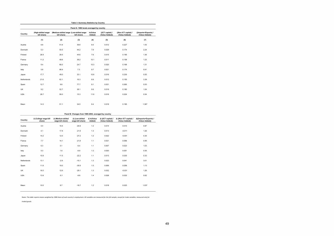
Panel A of Table 3 shows summary statistics for the levels of the key variables in

1980 across each country and Panel B presents the same for the changes through

2004. The levels have to be interpreted with care as exact comparison of qual-

ifications between countries is diffi cult, which is why wage bill shares are useful

summary measures as each qualification is weighted by its price (the wage)12.

The ranking of countries looks sensible with the US having the highest share of

high-skilled (29 percent), followed by Finland (27 percent). All countries have ex-

perienced significant skill upgrading as indicated by the growth in the high-skilled

wage bill share in column (1) of Panel B, on average the share increased form 14.3

12Estimating in differences also reduces the suspected bias from international

differences as the definitions are stable within country over time.

19

percent in 1980 to 24.3 in 2004.

The UK had the fastest absolute increase in the high-skilled wage bill share

(16.5 percentage points) and is also the country with the largest increase in ICT

intensity. The US had the second largest growth of ICT and the third largest

increase in the high-skilled wage bill share (13.9 percentage points), but all coun-

tries have experienced rapid increases in ICT intensity at the country level, which

doubled its 1980 share of value added. Figure 1 shows the correlation between

the growth of the wage bill share of each of the three education groups and ICT

intensity. There appears to be a positive relationship for the highly educated

(Figure 1A), a negative relationship for the middle educated (Figure 1B) and no

relationship for the least educated (Figure 1C). Although this is supportive of our

model’s predictions, there are many other unobservable influences at the country-

level for in our econometric results below will focus on the within country, across

industry variation.

Returning to Table 3, note that the change of the middle education share in

column (2) is more uneven. Although the mean growth is positive, it is relatively

small (8.7 percentage points on a base of 51.1 percent) compared to the highly

educated, with several countries experiencing no growth or a decrease (the US

and the Netherlands). The model in Appendix A shows how the wage bill share

20

of the middle-skilled could rise as the supply of this type of skill increases, so

this supply increase can offset the fall in relative demand caused by technical

change. Moreover, as Figure 2A shows, although the wage bill share of the middle

group rose more rapidly (in percentage point terms) between 1980 and 1986, it

subsequently decelerated. Indeed, in the last six year sub-period, 1998-2004, the

wage bill share of middle-skilled workers actually fell. At the same time, the wage

bill share of low-skilled workers continued to decline throughout the period 1980-

2004, but at an increasingly slower rate. Figure 2B shows the US, the technology

leader that is often a future indicator for other nations. From 1998-2004 the

wage bill share of the middle educated declined more rapidly than that of the

low-educated workers. Figure 2B is in line with the finding that while college

educated US workers continued to gain relative to high-school graduates, high-

school graduates gained relatively to college dropouts in the 1980s but not in the

1990s (see Autor, Katz and Kearney, 2008, Figure 5).

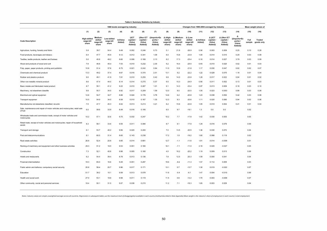
3.2.3. Cross Industry Trends

Table 4 breaks down the data by industry. In levels (column (1)) the highly

educated were disproportionately clustered into services both in the public sector

(especially education) and private sector (e.g. real estate and business services).

21

The industries that upgraded skills rapidly (column (8)) were also mainly services

(e.g. finance, telecoms and business services), but also in manufacturing (e.g.

chemicals and electrical equipment). At the other end of the skill distribution, the

textile industry, which initially had the lowest wage bill share of skilled workers,

upgraded somewhat more than other low-skill industries (transport and storage,

construction, hotels and restaurants, and agriculture). This raises the issue of

mean reversion, so we are careful to later show robustness tests to conditioning

on the initial levels of the skill shares in our regressions. In fact, the ranking

of industries in terms of skill intensity in 1980 and their skill upgrading over

the next 25 years was quite similar across countries. This is striking, because

the countries we analyze had different labor market institutions and different

institutional experiences over the period we analyze. This suggests something

fundamental is at play that cuts across different sets of institutions.

ICT grew dramatically from 1980-2004, accounting for more than 42 percent

of the average increase in capital services (see columns (12) and (13)). The in-

creased ICT diffusion was also quite uneven: financial intermediation and tele-

coms experienced rapid increases in ICT intensity, while in other industries, such

as agriculture, there was almost no increase.

Figures 3, 4, and 5 plot changes by industry in the wage bill shares of high,

22

medium, and low-skilled workers, respectively, against changes in ICT intensity.

The top panel (A) of each figure includes all industries with fitted regression

lines (solid line for all industry and dashed line for non-traded sectors only).

The bottom panel (B) restricts attention to the traded sectors. Figure 3A shows

that the industries with the fastest ICT upgrading had the largest increase in

the high-skilled wage bill share. One might be worried that two service sectors,

“Post & Telecommunications” and “Financial Intermediation”, are driving this

result, which is one reason Figure 3B drops all the non-traded sectors. In fact,

the relationship between high-skilled wage bill growth and ICT growth is actually

stronger in these “well measured”sectors.

Figure 4 repeats this analysis for the middle educated groups. We observe

the exact opposite relationship to Figure 3: the industries with the faster ICT

growth had the largest fall in the middle-skilled share whether we look at the

whole economy (Figure 4A) or just the traded sectors (Figure 4B). Finally, Figure

5 shows that there is essentially no relationship (Figure 5A) or a mildly positive

one (Figure 5B) between the change of the share of the least educated and ICT

growth.

These figures are highly suggestive of empirical support for the hypothesis that

ICT polarizes the skill structure: increasing demand at the top, reducing demand

23

in the middle and having little effect at the bottom. To examine this link more

rigorously, we now turn to the econometric analysis.

4. Econometric Results

4.1. Basic Results

Our first set of results for the skill share regressions are reported in Table 5. The

dependent variables are changes from 1980-2004 in the wage bill share of the high-

skilled in Panel A, the middle-skilled in Panel B and the low-skilled in Panel C.

The first four columns look across the entire economy and the last four columns

condition on the sub-sample of “tradable”sectors where we have information on

imports and exports.

Column (1) of Panel A reports the coeffi cient on the constant, which indicates

that on average there was a ten percentage point increase in the college wage bill

share. This is a very large increase, considering the average skill share in 1980

(across our sample of countries) was only 14%. Column (2) includes the growth in

ICT capital intensity. The technology variable has a large, positive and significant

coeffi cient and reduces the regression constant to 8.7. Column (3) includes the

growth of non-ICT capital intensity and value added. The coeffi cient on non-ICT

24

capital is negative and insignificant, suggesting that there is no sign of (non-ICT)

capital-skill complementarity. Some studies have found capital-skill complemen-

tarity (e.g. Griliches, 1969), but few of these studies have disaggregated capital

into its ICT and non-ICT components, so the evidence for capital-skill comple-

mentarity may be due to aggregating over high-tech capital that is complementary

with skills and lower tech capital that is not. The coeffi cient on value added growth

is positive and significant suggesting that skill upgrading has been occurring more

rapidly in the fastest growing sectors (as in Berman, Rohini and Tan, 2005). Col-

umn (4) includes country fixed effects. This is a demanding specification because

the specification is already in differences so this specification essentially allows for

country specific trends. The coeffi cient on ICT falls (from 65 to 47) but remains

significant at conventional levels13.

We re-estimate these specifications for the tradable industries in the next four

columns. Column (5) of Table 5 shows that the overall increase in the college

wage-bill share from 1980-2004 was 9 percentage points - similar to that in the

13Including the mineral extraction sectors caused the ICT coeffi cient to fall from

47 to 45. We also tried including a set of industry dummies in column (4). All

the variables became insignificant in this specification. This suggests that it is the

same industries that are upgrading across countries.

25

whole sample. Columns (6) - (8) add in our measure of ICT and other controls.

The coeffi cient on ICT in the tradable sector is positive, highly significant and

larger than in the overall sample (e.g. 129 in column (8)).

Panel B of Table 5 reports estimates for the same specifications as panel A,

but this time the dependent variable is the share of middle-educated workers.

The association between the change in middle-skilled workers and ICT is strongly

negative. In column (4), for example, a one percentage point increase in ICT

intensity is associated with a 0.8 percentage point fall in the proportion of middle-

skilled workers. The absolute magnitude of the coeffi cients for the sample that

includes all industries is quite similar to those for college educated workers. Panel

C shows that technology measures appear to be insignificant for the least educated

workers, illustrating the point that the main role of ICT appears to be in changing

demand between the high-skilled and middle-skilled groups14. Since the adding up

requirement means that the coeffi cients for the least skilled group can be deduced

from the other two skill groups we save space by omitting Panel C in the rest of

14The difference in the importance of ICT for the middle and lowest skill groups

implies that high school graduates are not perfect substitutes for college graduates

as Card (2009) argues in the US context. The majority of our data is from outside

the US, however, where there are relatively fewer high school graduates.

26

the Tables.

Overall, Table 5 shows a pattern of results consistent with ICT based polar-

ization. Industries where ICT grew most strongly where those with the largest

shifts towards the most skilled and the largest shifts away from the middle skilled,

with the least skilled largely unaffected.

4.2. Robustness and Extensions

4.2.1. Initial conditions

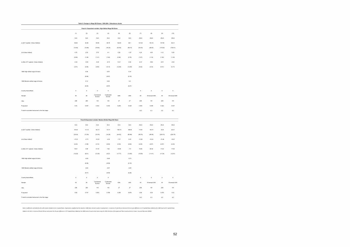
Table 6 examines some robustness checks using the results in our preferred speci-

fication of column (4) of Table 5 (reproduced in the first column). Since there may

be mean reversion we include the level of initial share of skills in 1980 in column

(2). This does not qualitatively alter the results, although coeffi cient on ICT for

the middle-skilled does fall somewhat15.15As we explain above our specifications assume that markets are national in

scope, so that country fixed effects capture changes in relative wages. To fur-

ther test this assumption we re-estimated columns (1) and (2) in Table 6 with

additional controls for the change in the difference in industry specific relative

ln(wages) between the high-skilled and middle-skilled and between the high-skilled

and low-skilled. The resulting coeffi cients (standard errors) on our measure of ICT

27

4.2.2. Timing of changes in skills and ICT

One limitation of the specifications that we discussed so far is that the changes

on the right-hand side and left hand-side are both concurrent. To mitigate po-

tential concerns about reverse causation, we re-estimate the baseline specification

of column (1) Table 6, where the right hand side variables are measured for the

first half of the period we consider (1980-1992) and the left hand side variable

is measured for the second half of the period (1992-2004). The estimated coeffi -

cients (and standard errors) on changes in our measure of ICT are 52.62 (23.53)

for high-skilled workers and -52.52 (28.97) for middle-skilled workers. These re-

sults are almost unchanged (51.31 (22.65) and -58.22 (22.99) respectively) when

we instead use the equivalent of the specification in column (2) of Table 6.

4.2.3. Heterogeneity in the coeffi cients across countries

Wage inequality rose less in Continental Europe than elsewhere, so it is interesting

to explore whether technological change induced polarization even there. Columns

(3) and (4) of Table 6 restrict the sample to the 8 Continental European countries

(Austria, Denmark, Finland, France, Germany, Italy, Netherlands and Spain),

are 41.43 (15.24) and 35.98 (14.82) for high-skilled workers, and -54.38 (20.96) and

-33.35 (13.87) for middle-skilled workers.

28

and the results are similar to those in the full sample of countries. In column

(5) we show that the correlation between ICT and polarization is larger for the

US than for the full sample, though column (6) shows that the estimates become

imprecise when we control for baseline levels of skill composition. The sample size

for most individual countries is rather small, but if we re-estimate the specification

of Table 5 column (2) separately country by country we obtain negative coeffi cients

on ICT for all 11 countries for medium skill shares and positive coeffi cients for 10

countries for the high skill shares (Japan is the single exception)16. The results

are also robust to dropping any single country17.

16The mean of the 11 country-specific coeffi cients on ICT is very similar to the

pooled results (-112 for the middle-skilled share and 71 for the high-skilled share).17For example, we had concerns about the quality of the education data in Italy

so we dropped it from the sample. In the specification of column (4) of Table 5, the

coeffi cient (standard error) on ICT capital was 55.2(1.04) for the high education

group and -68.54(22.82) for the middle educated.

29

4.2.4. Instrumental variables

One concern is that measurement error in the right hand side variables, especially

our measure of ICT, causes attenuation bias18. To mitigate this concern, we use

the industry-level measures of ICT in the US in 1980 as an instrument for ICT

upgrading over the whole sample. The intuition behind this instrument is that

the dramatic global fall in quality-adjusted ICT prices since 1980 (e.g. Jorgenson,

Ho and Stiroh, 2008) disproportionately affects industries that (for exogenous

technological reasons) have a greater potential for using ICT inputs. An indicator

of this potential is the initial ICT intensity in the technological leader, the US. As

column (7) of Table 6 shows, this instrument has a first-stage F-statistic of 10.5,

and the sign of the first stage regressions (not reported) is as we would expect,

namely that industries that were more ICT-intensive in 1980 upgraded their use

18Estimates of the ICT coeffi cient for the two 12-year sub-periods of our data are

typically about half of the absolute magnitude of those for the full period. In gen-

eral, our estimates for shorter time periods are smaller and less precise, consistent

with the importance of measurement error in the ICT data. For example, in the

specification of column (4) of Panel A in Table 5, the coeffi cient (standard error)

on ICT was 18.30 (10.30) in a pooled 12 year regression. We could not reject the

hypothesis that the ICT coeffi cient was stable over time (p-value=0.35).

30

of ICT more than others. In the 2SLS estimates of column (7) the coeffi cient

on ICT is roughly twice as large as the OLS coeffi cients for the college educated

group (and significant at the 5 percent level), and a little bigger for the middle-

skilled group. Column (8) report estimates the same specification but this time

excluding the US itself, and the results are very similar. While we acknowledge

that estimates using this instrument do not necessarily uncover the causal effect

of ICT, it is reassuring that these 2SLS estimates are somewhat larger than the

OLS estimates, as we would expect given the likely measurement error.

As a further check, we use the proportion of routine tasks in the industry (in

the US in the base year) as an instrument for future ICT growth as these industries

were most likely to be affected by falling ICT prices (see Autor and Dorn, 2009).

The results of using this instrument are shown in columns (9) and (10). Although

the first stages are weaker with this instrument19, and the 2SLS estimates are

not very precise, these columns again suggest that we are not over-estimating the

importance of ICT by just using OLS.

19The signs of the instruments in the first stage are correct. The F-test is 6.5 in

column (9) compared to 10.5 in column (7).

31

4.2.5. Disaggregating the wage bill into wages and hours

The wage bill share of each skill group reflects its hourly wage and hours worked,

and those of the other skill groups. We estimated specifications that are identical

to those in Table 5, except that they disaggregate the dependent variable into the

growth of relative skill prices and quantities. In the first two columns of Table 7

we reproduce the baseline specifications using the log relative wage bill (which can

be exactly decomposed) as the dependent variable20. Columns (1) - (4) confirm

what we have already seem using a slightly different functional form: ICT growth

is associated with a significant increase in the demand for high-skilled workers

relative to middle-skilled workers (first two columns) and with a significant (but

smaller) increase for low-skilled workers relative to middle-skilled workers (third

and fourth columns).

For the high vs. middle-skill group, ICT growth is significantly associated with

increases in relative wages and relative hours (columns (5), (6), (9) and (10)). In

20Another functional form check was using the growth rate of ICT intensity. For

the specification in column (3) of Panel A in Table 5 we replaced ∆(C/Q) with

∆(C/Q)C/Q

. The coeffi cient (standard error) on ICT growth was 2.586 (1.020). The

marginal effect of a one standard deviation increase (0.581) is 1.50 (=0.581*2.586),

almost identical to 1.55 (=0.024*64.6) in Table 5.

32

comparing the middle vs. low groups, the coeffi cients are also all correctly signed,

but not significant at conventional levels. Overall this suggests that our results

are robust to functional form and the shifting pattern of demand operates both

through wages and hours worked21.

4.3. Trade, R&D and skill upgrading

Having found that technology upgrading is associated with substitution of college-

educated workers for middle-educated workers, we now examine whether changes

in trade exhibit similar patterns. The first three columns of Table 8 suggest

that more trade openness (measured as the ratio of imports plus exports to value

added) is associated with increases in the wage bill share of college educated work-

ers and declines in the share for middle-skilled workers. However, the when we

control for initial R&D intensity the association between trade and skill upgrad-

ing becomes smaller and insignificant. Column (4) repeats the specification of

column (3) for the sub-sample where we have R&D data and shows that the trade

21In examining these results across countries there was some evidence that the

adjustment in wages was stronger in the US and the adjustment in hours was

stronger in Continental Europe. This is consistent with the idea of great wage

flexibility in the US than in Europe.

33

coeffi cient is robust. Column (5) includes R&D intensity in a simple specification

and shows that the coeffi cient on trade falls (e.g. from 0.50 to 0.24 in Panel A)

and is insignificant, whereas the coeffi cient on R&D is positive and significant. In

column (6) we include the changes in the ICT and non-ICT capital stocks and the

coeffi cient on trade is now very small. Column (7) drops the insignificant trade

variable and shows that ICT and R&D and individually (and jointly) significant.

We also used the Feenstra and Hansen (1999) method of constructing an off-

shoring variable and included it instead of (and alongside) trade in final goods.

The offshoring variable has a bit more explanatory power than final goods trade22.

Column (8) includes offshoring (“Imported Intermediate Inputs”) into the full

sample as it can be defined for all industries. The results suggest a significant

positive correlation between offshoring for high skilled workers and a negative but

insignificant correlation between ICT and demand for middle skilled workers. Col-

umn (9) produces a similar result on the sample of tradable sectors and column

(10) includes ICT and R&D. As with the trade measure in final goods, the off-

22For example, in the same specification of column (6) of Table 8 we replaced

the final goods trade variable with the offshoring measure. In the high skilled

equation the coeffi cient (standard error) was 4.27 (2.82) and in the middle skilled

equation the coeffi cient (standard error) was -11.6 (9.87).

34

shoring coeffi cient is insignificant in the final column for both education groups.

The ICT effects are robust to the inclusion of the offshoring measures.

These findings are broadly consistent with most of the literature that finds

that technology variables have more explanatory power than trade in these kinds

of skill demand equations23. Of course, trade could be influencing skill demand

through affecting the incentives to innovate and adopt new technologies, which is

why trade ceases to be important after we condition on technology (e.g. Draca,

Bloom and Van Reenen, 2011, argue in favor of this trade-induced technical change

hypothesis)24. Furthermore, there could be many general equilibrium effects of

trade that we have not accounted for (these are controlled for by the country time23These are simple industry-level correlations and not general equilibrium cal-

culations, so we may be missing out the role of trade through other routes.24We further test whether the association between trade and skill upgrading

remains similar when we examine different components of trade separately. Ap-

pendix Table A3 suggests that when we examine imports and exports separately,

the picture is quite similar. Greater trade is associated with an increase in the

college wage bill share until we control for initial R&D intensity, in which case the

coeffi cient on trade falls and becomes insignificant. Results are similar when we

analyze separately imports to (or exports from) OECD countries. For non-OECD

countries the results are again the same, except for exports to non-OECD coun-

35

effects).

4.4. Magnitudes

We perform some “back of the envelope”calculations (see Table A4) to gauge the

magnitude of the effect of technology on the demand for highly skilled workers.

Column (1) estimates that ICT accounts for 13.2 percent of the increase in the

college share in the whole sample without controls and column (2) reduces this to

8.5 percent with controls. Many authors (e.g. Jorgenson, Ho and Stiroh, 2008)

have argued that value added growth has been strongly affected by ICT growth,

especially in the later period, so column (2) probably underestimates the effect of

ICT. Column (3) reports equivalent calculations for the tradable sectors. Here,

ICT accounts for 16.5 percent of the change and R&D a further 16.1 percent,

suggesting that observable technology measures by account for almost a third of

the increase in demand for highly skilled workers. If we include controls in column

(4) this falls to 23.1 percent. Finally, columns (5) and (6) report results for the

IV specification for the whole sample, showing an ICT contribution of ICT of

tries, which remains positively associated with changes in the college wage-bill

share even after we add all the controls, including R&D. However, it should be

noted that the change in exports to developing countries is on average very small.

36

between 22.1 percent and 27.7 percent25.

We also note that while ICT upgrading alone should have led to decreased

demand for middle-skilled workers. While we do not see such a decrease overall,

Figure 2 shows a slowdown in the growth of demand for middle skilled over time,

and a reversal (in other words negative growth) for middle-skilled workers from

1998-2004.

We have no general equilibrium model, so these are only “back of the enve-

lope”calculations to give an idea of magnitudes. Furthermore, measurement error

probably means that we are probably underestimating the importance of the vari-

ables. Nevertheless, it seems that our measures of technology are important in

explaining a significant proportion of the increase in demand for college educated

workers at the expense of the middle-skilled.

25The IV specifications for tradeables show an even larger magnitude. For ex-

ample in a specification with full controls, R&D and ICT combined account for

over half of all the change in the college wage bill share. The first stage for the

IV is weak, however, with an F-statistic of 6, these cannot be relied on.

37

5. Conclusions

Recent investigations into the changing demand for skills in OECD countries have

found some evidence for “polarization” in the labour market in the sense that

workers in the middle of the wage and skills distribution appear to have fared

more poorly than those at the bottom and the top. One explanation that has

been advanced for this is that ICT has complemented non-routine analytic tasks

but substituted for routine tasks whilst not affecting non-routine manual tasks

(like cleaning, gardening, childcare, etc.). This implies that many middle-skilled

groups like bank clerks and paralegals performing routine tasks have suffered a

fall in demand. To test this we have estimated industry-level skill share equations

distinguishing three education groups and related this to ICT (and R&D) invest-

ments in eleven countries over 25 years using newly available data. Our findings

are supportive of the ICT-based polarization hypothesis as industries that experi-

enced the fastest growth in ICT also experienced the fastest growth in the demand

for the most educated workers and the fastest falls in demand for workers with

intermediate levels of education. The magnitudes are nontrivial: technical change

can account for up to a quarter of the growth of the college wage bill share in the

economy as a whole (and more in the tradable sectors).

38

Although our method is simple and transparent, there are many extensions

that need to be made. First, alternative instrumental variables for ICT would

help identify the causal impact of ICT. Second, although we find no direct role

for trade variables, there may be other ways in which globalization influences the

labour market, for example by causing firms to “defensively innovate”(Acemoglu,

2003). Third, there are alternative explanations for the improved performance of

the least skilled group through for example, greater demand from richer skilled

workers for the services they provide as market production substitutes for house-

hold production (e.g. childcare, eating out in restaurants, domestic work, etc.)26.

These explanations may complement the mechanism that we address here. Finally,

we have not used richer occupational data that would focus on the skill content of

tasks due to the need to have international comparability across countries. The

work of Autor and Dorn (2009) is an important contribution here.

26See Ngai and Pissarides (2007) and Mazzolari and Ragusa (2008).

39

References

Acemoglu, Daron (2003) “Patterns of Skill Premia”Review of Economic Stud-

ies, 70(2): 199—230.

Acemoglu, Daron and David Autor (2010) “Skills, Tasks and Technologies:

Implications for Employment and Earnings”Handbook of Labor Economics Vol-

ume IV edited by David Card and Orley Ashenfelter, Princeton: Princeton Uni-

versity Press

Autor, David, and Alan Krueger, (1998) “Computing Inequality: Have Com-

puters Changed the Labor Market?”Quarterly Journal of Economics, 113 (4),

1169-1214

Autor, David , Lawrence Katz and Melissa Kearney (2006) “The Polar-

ization Of The U.S. Labor Market”American Economic Review 96(2), 189-194,

Autor, David , Lawrence Katz andMelissa Kearney (2008) “Trends in U.S.

Wage Inequality: Revising the Revisionists”Review of Economics and Statistics

90(2), 300-323

Autor, David, Frank Levy and Richard Murnane (2003) “The Skill Content

Of Recent Technological Change: An Empirical Exploration”Quarterly Journal

40

of Economics, 118(4), 1279-1333

Autor, David and David Dorn (2009) “Inequality and Specialization: The

Growth of Low-Skill Service Jobs in the United States”NBER Working Paper

15150

Berman, Eli, John Bound and Zvi Griliches (1994) “Changes in the demand

for skilled labor within US manufacturing industries: Evidence from the Annual

Survey of Manufacturing”, Quarterly Journal of Economics, 109, 367-98.

Berman, Eli, Rohini Somanathan and Hong Tan. (2005). “Is skill-biased

technological change here yet? Evidence from Indian manufacturing in the 1990s”

Annales d’Economie et de Statistique, 79-80, 299-321.

Black, Sandra and Alexandra Spitz-Oener (2010). “Explaining Women’s

Success: Technological Change and the Skill Content of Women’s Work”Review

of Economics and Statistics 92(1), 187-194.

Bloom, Nick, Mirko Draca and John Van Reenen (2011) “Trade Induced

Technical Change? The impact of Chinese imports on technology, jobs and plant

survival”, NBER Working Paper No. 16717

Bond, Stephen and John Van Reenen (2007) “Micro-econometric models of

41

investment and employment”Chapter 65 in Heckman, J. and Leamer. E. (eds)

Handbook of Econometrics Volume 6A, 4417-4498

Brown, Randall and Laurits Christensen (1981), “Estimating elasticities

of substitution in a model of partial static equilibrium: an application to US

agriculture 1947-74”, in: C. Field and E. Berndt, eds., Modelling and Measuring

Natural Resource Substitution (MIT Press, Cambridge).

Card, David (2009) “Immigration and Inequality”, American Economic Review,

99(2), 1-21

Desjonqueres, Thibaut, Stephen Machin, and John Van Reenen (1999)

“Another Nail in the Coffi n? Or Can the Trade Based Explanation of Changing

Skill Structures Be Resurrected?”The Scandinavian Journal of Economics, 101

(4), 533-554.

DiNardo, John, Nicole Fortin and Thomas Lemieux (1996) “Labor Mar-

ket Institutions and the Distribution of Wages, 1973-1992: A Semiparametric

Approach”Econometrica 64(5), 1001-1044.

DiNardo, John and Jorn-Steffen Pischke (1997) “The Returns to Computer

Use Revisited: Have Pencils Changed the Wage Structure Too?”Quarterly Jour-

nal of Economics 112(1), 291-303

42

Dustmann, Christian, Johannes Ludsteck and Uta Schonberg (2009)

“Revisiting the GermanWage Structure.”Quarterly Journal of Economics, 124(2),

843-881.

Feenstra, Robert and Gordon Hanson. (1996) “Foreign Investment, Out-

sourcing and Relative Wages”in Robert Feenstra and Gene Grossman, eds., Polit-

ical Economy of Trade Policy: Essays in Honor of Jagdish Bhagwati, Cambridge

MA: MIT Press.

Firpo, Sergio, Nicole Fortin and Thomas Lemieux (2011) “Occupational

Tasks and Changes in the Wage Structure”IZA Discussion Paper 5542.

Goldin, Claudia and Lawrence Katz (2008) The Race between Education and

Technology. Cambridge, MA: Harvard University Press

Goos, Maarten, Alan Manning and Anna Salomons (2009) “Job Polariza-

tion in Europe”, American Economic Review, 99(2), 58-63.

Goos, Maarten, Alan Manning and Anna Salomons (2010) “Explaining

Job Polarization in Europe: The Roles of Technology and Globalization”, Univer-

sity of Maastricht, mimeo.

Goos, Maarten and Alan Manning (2007) “Lousy and Lovely Jobs: The

43

Rising Polarization of Work in Britain”Review of Economics and Statistics, 89(1),

118-133

Griliches, Zvi (1969) “Capital-Skill complementarity”Review of Economics and

Statistics 51:465-468.

Jorgenson, Dale, Mun Ho, and Kevin Stiroh (2008) “A Retrospective Look

at the US Productivity Growth Resurgence”, Journal of Economic Perspectives,

22(1), 3-24.

Krueger, Alan (1993) “How computers have changed the wage structure”, Quar-

terly Journal of Economics., 108, 33-60.

Krugman, Paul. (2008) “Trade and Wages reconsidered”, Brookings Papers on

Economic Activity, Spring, 103-154

Machin, Stephen and John Van Reenen (1998) “Technology and Changes

in Skill Structure: Evidence from Seven OECD Countries”Quarterly Journal of

Economics 113, 1215-44.

Matsuyama, Kiminori. (2007) “Beyond Icebergs: Towards a Theory of Biased

Globalization”Review of Economic Studies 74, 237—253

Mazzolari, Francesca and Giuseppe Ragusa (2008) “Spillovers from High-

44

Skill Consumption to Low-Skill Labor Markets.”Mimeograph, University of Cal-

ifornia at Irvine

Ngai, L. Rachel and Christopher Pissarides (2007) “Structural Change in

a Multisector Model of Growth.”American Economic Review, 97(1), 429-443.

O’Mahony, Mary and Marcel P. Timmer (2009) “Output, Input and Pro-

ductivity Measures at the Industry Level: the EU KLEMS Database”, Economic

Journal, 119(538), F374-F403

Spitz-Oener, Alexandra (2006) “Technical Change, Job Tasks, and Rising Ed-

ucational Demands: Looking Outside the Wage Structure,”Journal of Labor Eco-

nomics 24(2) 235—270.

Smith, Christopher L. (2008) “Implications of Adult Labor Market Polariza-

tion for Youth Employment Opportunities.”MIT working paper

Timmer, Marcel, Ton van Moergastel, Edwin Stuivenwold , Gerard

Ypma, Mary O’Mahony andMari Kangasniemi (2007) “EUKLEMSGrowth

and Productivity Accounts Version 1.0”, University of Groningen mimeo

Timmer, Marcel, Robert Inklaar, Mary O’Mahony and Bart van Ark

(2010) Economic Growth in Europe Cambridge: Cambridge University Press

45

Wood, Adrian. (1994) North-South Trade, Employment and Inequality, Chang-

ing Fortunes in a Skill-Driven World, Clarendon, Oxford.

46

Cognitive Manual Manual

occ8090 occupation description

Set limits, Tolerances, or

StandardsFinger

Dexterity

Quantitative reasoning

requirements

Direction, Control, and

PlanningEye-Hand-Foot

coordination

Top 10 occupations ranked by share of high-skilled workers

84 Physicians 460,260 0.97 0.03 0.00 -0.96 4.18 1.94 1.87 0.50

178 Lawyers 534,780 0.95 0.05 0.00 -0.96 -1.11 1.05 -0.51 -0.80

85 Dentists 135,620 0.94 0.06 0.00 1.47 4.73 1.99 -0.55 0.89

133 Medical science teachers 9,860 0.93 0.06 0.01 -1.05 -0.90 1.73 2.08 -0.80

126 Social science teachers, n.e.c. 2,480 0.93 0.04 0.03 -1.05 -1.12 2.01 2.33 -0.80

146 Social work teachers 1,060 0.92 0.06 0.02 -1.05 -1.12 2.01 2.33 -0.80

123 History teachers 6,380 0.92 0.06 0.02 -1.05 -1.12 1.73 2.17 -0.80

118 Sociology teachers;Psychology teachers 9,200 0.92 0.06 0.02 -1.05 -1.12 2.01 2.33 -0.80

147 Theology teachers 3,940 0.91 0.07 0.03 -1.05 -1.12 1.97 2.27 -0.80

86 Veterinarians 37,440 0.91 0.08 0.01 1.00 4.06 0.96 -0.52 -0.71

Top 10 occupations ranked by share of middle-skilled workers

314 Stenographers 106,360 0.07 0.88 0.05 1.40 1.13 -0.58 -0.64 -0.80

529 Telephone installers and repairers 273,980 0.03 0.87 0.10 1.45 1.38 0.47 -0.60 2.16

383 Bank tellers 639,180 0.07 0.86 0.07 1.48 2.53 0.29 -0.49 -0.80

313 Secretaries 5,020,140 0.08 0.86 0.07 -0.71 2.73 0.17 -0.61 -0.79

385 Data-entry keyers 472,880 0.05 0.85 0.10 1.31 0.23 0.08 0.16 -0.76

206 Radiologic technicians 110,060 0.10 0.85 0.04 1.51 0.98 1.13 -0.59 0.92

527 Telephone line installers and repairers 65,560 0.03 0.85 0.12 1.32 1.06 0.34 -0.37 1.80

315 Typists 969,040 0.05 0.84 0.11 -0.06 1.50 -0.12 -0.63 -0.76

338 Payroll and timekeeping clerks 200,940 0.06 0.83 0.11 1.47 0.79 0.05 -0.52 -0.80

525 Data processing equipment repairers 48,140 0.10 0.83 0.06 1.43 1.19 0.81 -0.34 -0.70

Top 10 occupations ranked by share of low-skilled workers

407 Private household cleaners and servants 569,980 0.02 0.27 0.71 -1.05 -1.12 -0.86 -0.58 0.54

488 Graders and sorters, agricultural products 40,100 0.01 0.30 0.69 -0.04 -0.42 -0.87 -0.49 0.78

404 Cooks, private household 18,460 0.03 0.30 0.67 -1.05 -1.12 -0.80 -0.38 -0.14

747 Pressing machine operators 145,740 0.01 0.33 0.67 -0.91 0.16 -1.47 -0.66 0.42

405 Housekeepers and butlers 101,220 0.02 0.32 0.65 -1.05 -1.12 -0.83 0.04 0.28

738 Winding and twisting machine operators 140,080 0.01 0.35 0.65 0.51 0.69 -1.46 -0.61 -0.11

403 Launderers and Ironers 3,160 0.02 0.34 0.65 -1.05 -1.12 -1.49 -0.66 0.25

479 Farm workers 1,337,020 0.03 0.33 0.64 -0.03 -0.39 -0.87 -0.49 0.78

443 Waiters'/waitresses' assistants 422,800 0.01 0.36 0.62 -1.01 -0.98 -1.34 -0.64 0.73

449 Maids and housemen 969,720 0.01 0.36 0.62 -0.98 -1.05 -1.33 -0.47 0.38

Table 1: Top occupations by share of workers of different skill levels, with task measures

Employment in 1980

Fraction high-skilled

Fraction middle-skilled

Fraction low-

skilled

Standardized skill measures

Routine tasks Non routine tasks

Cognitive

Note: This table reports the top 10 occupations for each of the three skill categories, along with mean standardized task measures, using 1980 US Census micro data and the occ8090 classification from Autor,

Levy, and Murnane (2003). For each task measure, the standardized measure is derived by subtracting from each occupation's task score the weighted mean task score across all occupations, and then dividing

the difference by the standard deviation of the task measure across the 453 occupations.

47

High-skilled Middle-skilled Low-skilled

Cognitive Set limits, Tolerances, or Standards -0.32 0.06 0.07

Manual Finger Dexterity -0.21 0.13 -0.14

Quantitative reasoning requirements 0.79 -0.02 -0.43

Direction, Control, and Planning 0.90 -0.11 -0.32

Manual Eye-Hand-Foot coordination -0.36 -0.04 0.29

Table 2: Mean Standardized Scores by skill group - 1980 US data

Routine tasks

Non routine tasks

Cognitive

Note: This table reports the mean standardized task measures by skill group, using 1980 US Census micro data and the occ8090 classification from

Autor, Levy, and Murnane (2003). For each task measure, the standardized measure is derived by subtracting from each occupation's task score the

weighted mean task score across all occupations, and then dividing the difference by the standard deviation of the task measure across the 453

occupations.

48

Country(High-skilled wage-

bill share)(Medium-skilled wage-

bill share)(Low-skilled wage-

bill share)ln(Value Added)

((ICT capital) / (Value Added))

((Non ICT capital) / (Value Added))

((Imports+Exports) / (Value Added))

(1) (2) (3) (4) (5) (6) (7)

Austria 8.8 51.6 39.6 8.0 0.012 0.227 1.43

Denmark 5.3 50.5 44.2 7.8 0.029 0.174 2.24

Finland 26.9 28.5 44.6 7.6 0.015 0.195 1.36

France 11.2 49.6 39.2 10.1 0.011 0.158 1.23

Germany 9.4 66.0 24.7 10.3 0.020 0.168 1.31

Italy 5.8 86.9 7.3 9.7 0.021 0.174 0.91

Japan 17.7 49.0 33.1 10.8 0.016 0.230 0.55

Netherlands 21.6 62.1 16.3 8.8 0.012 0.155 3.39

Spain 12.7 9.6 77.7 9.1 0.021 0.265 0.53

UK 9.2 52.7 38.1 9.8 0.019 0.180 1.54

USA 28.7 56.0 15.3 11.6 0.016 0.224 0.54

Mean 14.3 51.1 34.5 9.4 0.018 0.195 1.367

Country∆ (College wage-bill

share)∆ (Medium-skilled wage-bill share)

∆ (Low-skilled wage-bill share)

∆ ln(Value Added)

∆ ((ICT capital) / (Value Added))

∆ ((Non ICT capital) / (Value Added))

∆((Imports+Exports) / (Value Added))

Austria 5.4 15.5 -20.9 1.2 0.014 0.010 0.87

Denmark 4.1 17.8 -21.9 1.3 0.013 -0.011 1.26

Finland 15.2 12.0 -27.2 1.2 0.022 -0.001 0.35

France 7.7 14.1 -21.8 1.1 0.021 0.066 0.99

Germany 6.3 0.1 -6.4 1.1 0.007 0.023 1.03

Italy 5.3 1.6 -6.9 1.2 0.020 0.051 0.55

Japan 10.8 11.5 -22.2 1.1 0.013 0.035 0.33

Netherlands 13.1 -2.9 -10.1 1.3 0.023 0.041 3.01

Spain 11.9 19.0 -30.9 1.5 0.006 0.056 1.13

UK 16.5 12.6 -29.1 1.3 0.032 -0.031 1.26

USA 13.9 -5.1 -8.8 1.4 0.028 0.032 0.62

Mean 10.0 8.7 -18.7 1.2 0.018 0.025 1.037

Panel A: 1980 levels averaged by country

Table 3: Summary Statistics by Country

Panel B: Changes from 1980-2004, averaged by country

Notes: The table reports means weighted by 1980 share of each country's employment. All variables are measured for the full sample, except for trade variables, measured only for

traded goods.

49

(1) (2) (3) (4) (5) (6) (7) (8) (9) (10) (11) (12) (13) (14) (15) (16)

Code DescriptionHigh-skilled

wage-bill share

Medium-skilled

wage-bill share

Low-skilled wage-bill

share

ln(Value Added)

((ICT capital) / (Value

Added))

((Non ICT capital) / (Value

Added))

((Imports+Exports) / (Value

Added))

∆ (High-skilled

wage-bill share)

∆ (Medium-skilled

wage-bill share)

∆ (Low-skilled

wage-bill share)

∆ ln(Value Added)

∆ ((ICT capital) / (Value

Added))

∆ ((Non ICT capital) / (Value

Added))

∆ ((Imports+Ex

ports) / (Value

Added))

Full sample

Traded goods only

Agriculture, hunting, forestry and fishing 5.9 39.7 54.4 9.49 0.002 0.246 0.73 5.1 21.8 -26.9 0.56 0.003 0.009 0.25 0.10 0.28

Food products, beverages and tobacco 6.4 47.7 45.9 9.12 0.012 0.341 1.09 8.0 15.8 -23.9 1.00 0.014 0.010 0.29 0.03 0.09

Textiles, textile products, leather and footwea 5.0 45.8 49.2 8.60 0.006 0.168 2.13 8.2 17.3 -25.4 0.16 0.014 0.027 3.79 0.03 0.09

Wood and products of wood and cork 7.8 46.8 45.4 7.53 0.010 0.232 2.30 9.2 16.4 -25.5 0.93 0.010 0.020 0.02 0.01 0.03

Pulp, paper, paper products, printing and publishin 10.8 51.4 37.8 8.75 0.021 0.242 0.84 11.0 10.9 -21.8 1.17 0.030 0.047 0.02 0.02 0.07

Chemicals and chemical products 13.3 49.2 37.4 8.67 0.016 0.370 2.51 13.1 9.2 -22.2 1.22 0.028 0.070 1.18 0.01 0.04

Rubber and plastics products 9.0 49.1 41.9 7.81 0.010 0.255 0.42 9.8 14.0 -23.8 1.28 0.017 0.022 0.04 0.01 0.02

Other non-metallic mineral products 8.6 47.4 44.0 8.14 0.014 0.270 0.57 9.5 15.3 -24.9 0.90 0.011 0.052 0.13 0.01 0.03

Basic metals and fabricated metal products 8.7 50.1 41.2 9.22 0.010 0.267 1.01 9.1 14.3 -23.4 0.97 0.013 0.009 0.18 0.03 0.10

Machinery, not elsewhere classified 9.8 55.7 34.5 8.92 0.017 0.209 1.59 12.0 8.5 -20.5 1.05 0.023 -0.003 0.98 0.03 0.08

Electrical and optical equipmen 12.6 54.7 32.7 8.88 0.024 0.176 3.78 14.6 6.2 -20.8 1.23 0.038 0.052 5.42 0.03 0.08

Transport equipment 10.5 54.9 34.5 8.58 0.010 0.167 1.35 12.3 8.3 -20.6 1.11 0.020 0.080 0.94 0.02 0.06

Manufacturing not elsewhere classified; recyclin 7.0 47.7 45.3 8.02 0.013 0.213 3.21 8.2 15.6 -23.8 1.05 0.010 0.004 0.41 0.01 0.04

Sale, maintenance and repair of motor vehicles and motorcycles; retail sale of fuel 6.5 59.6 33.9 8.49 0.016 0.195 8.5 9.7 -18.1 1.3 0.0 0.0 0.02

Wholesale trade and commission trade, except of motor vehicles and motorcycles 10.2 57.1 32.6 9.70 0.032 0.247 10.2 7.7 -17.8 1.42 0.030 0.055 0.05

Retail trade, except of motor vehicles and motorcycles; repair of household goods 8.3 58.1 33.6 9.55 0.011 0.084 8.7 9.1 -17.8 1.29 0.016 0.079 0.09

Transport and storage 6.1 53.7 40.2 9.56 0.020 0.200 7.0 13.5 -20.5 1.36 0.030 0.072 0.04

Post and telecommunications 8.1 60.5 31.4 8.65 0.143 0.238 17.2 1.9 -19.2 1.60 0.088 0.119 0.02

Real estate activities 26.8 52.4 20.8 9.85 0.014 0.891 12.7 -1.1 -11.6 1.81 0.014 -0.008 0.01

Renting of machinery and equipment and other business activities 29.3 51.2 19.5 9.53 0.051 0.180 18.1 -7.1 -11.0 2.16 0.020 -0.027 0.05

Construction 7.3 52.1 40.6 9.98 0.005 0.180 4.0 16.2 -20.2 1.19 0.009 0.013 0.08

Hotels and restaurants 6.2 54.4 39.4 8.78 0.013 0.136 7.8 12.5 -20.3 1.59 0.000 0.041 0.04

Financial intermediation 18.3 65.0 16.6 9.49 0.051 0.297 19.6 -8.2 -11.3 1.57 0.112 0.009 0.03

Public admin and defence; compulsory social security 20.8 58.4 20.7 9.96 0.017 0.171 13.1 0.7 -13.7 1.30 0.019 -0.022 0.07

Education 51.7 38.2 10.1 9.58 0.013 0.078 11.6 -5.4 -6.1 1.47 0.004 -0.010 0.06

Health and social work 27.0 53.1 19.8 9.58 0.011 0.119 11.5 0.8 -12.2 1.70 0.003 -0.008 0.07

Other community, social and personal services 18.4 50.1 31.5 9.07 0.038 0.215 11.2 7.1 -18.3 1.65 0.003 0.029 0.04

1980 levels averaged by industry Mean weight (share of

Table 4: Summary Statistics by Industry

Changes from 1980-2004 averaged by industry

Notes: Industry values are simple unweighted averages across all countries. Regressions in subsequent tables use the maximum level of disaggregation available in each country (method described in Data Appendix).Mean weight is the industry’s share of employment in each country’s total employment

50

(1) (2) (3) (4) (5) (6) (7) (8)

∆ ((ICT capital) / (Value Added)) 72.29 64.56 46.92 163.94 139.6 128.71

(18.28) (17.31) (14.94) (45.48) (42.74) (32.19)

∆ ln(Value Added) 5.42 4.76 3.26 3.41

(1.24) (0.95) (2.25) (1.07)

∆ ((Non ICT capital) / (Value Added)) -7.64 -6.45 0.31 -0.47

(4.92) (3.51) (5.59) (2.45)

Intercept 10.02 8.69 2.22 9.12 6.42 4.04

(0.57) (0.63) (1.68) (0.86) (1.02) (2.19)

Country fixed effects X X

Sample: All industries X X X X

Sample: Traded industries X X X X

Obs. 208 208 208 208 84 84 84 84

R-squared 0.09 0.20 0.45 0.20 0.23 0.81

∆ ((ICT capital) / (Value Added)) -100.78 -77.76 -64.52 -163.98 -41.59 -288.01

(30.21) (25.44) (20.24) (115.78) (84.73) (83.94)

∆ ln(Value Added) -13.8 -15.33 -15.64 -7.96

(2.69) (2.23) (4.27) (3.14)

∆ ((Non ICT capital) / (Value Added)) 9.76 18.01 -10.79 1.57

(11.88) (10.25) (14.08) (10.98)

Intercept 8.73 10.59 27.24 15.5 18.20 29.75

(1.29) (1.49) (3.73) (1.90) (2.95) (4.67)

Country fixed effects X X

Sample: All industries X X X X

Sample: Traded industries X X X X

Obs. 208 208 208 208 84 84 84 84

R-squared 0.05 0.23 0.58 0.05 0.25 0.74

∆ ((ICT capital) / (Value Added)) 28.55 13.21 17.71 0.50 -97.91 159.65

(27.34) (25.66) (16.41) (113.51) (100.71) (79.30)

∆ ln(Value Added) 8.43 10.62 12.45 4.61

(2.40) (1.95) (4.24) (3.30)

∆ ((Non ICT capital) / (Value Added)) -2.21 -11.68 10.32 -1.28

(9.63) (9.07) (11.91) (11.73)

Intercept -18.74 -19.26 -29.5 -24.61 -24.62 -33.84

(1.12) (1.31) (3.27) (1.68) (2.56) (3.95)

Country fixed effects X X

Sample: All industries X X X X

Sample: Traded industries X X X X

Obs. 208 208 208 208 84 84 84 84

R-squared 0.01 0.10 0.65 0.00 0.16 0.70

Table 5: Changes in Wage Bill Shares: 1980-2004

Panel B:Dependent variable: Medium-skilled Wage Bill Share

Panel A:Dependent variable: High-Skilled Wage Bill Share

Panel C:Dependent variable: Low-skilled Wage Bill Share

Notes: Coefficients estimated by OLS with robust standard errors in parentheses. Regressions in columns (1)-(4) weighted by each industry's 1980

share of each country's employment, and regressions in columns (5)-(8) weighted by each industry's 1980 share of each country's employment in

traded industries. Columns (1)-(4) are estimated on all industries and columns (5)-(8) are on the tradable sectors.

51

(1) (2) (3) (4) (5) (6) (7) (8) (9) (10)

OLS OLS OLS OLS OLS OLS 2SLS 2SLS 2SLS 2SLS

∆ ((ICT capital) / (Value Added)) 46.92 42.09 50.98 48.79 132.84 66.1 121.63 103.16 137.99 65.31

(14.94) (14.66) (16.64) (16.20) (52.59) (58.15) (53.43) (48.82) (119.44) (104.61)

∆ ln(Value Added) 4.76 2.93 5.79 4.4 0.26 -1.97 4.24 4.85 4.12 5.09

(0.95) (1.39) (1.31) (1.93) (2.94) (3.79) (1.07) (1.10) (1.30) (1.20)

∆ ((Non ICT capital) / (Value Added)) -6.45 -5.06 -9.25 -8.19 15.41 2.56 -8.47 -9.85 -8.91 -8.54

(3.51) (3.99) (4.56) (5.13) (12.99) (12.95) (4.02) (4.33) (5.01) (5.17)

1980 High-skilled wage bill share 0.06 0.04 0.34

(0.06) (0.07) (0.19)

1980 Medium-skilled wage bill share 0.12 0.08 0.6

(0.05) (0.07) (0.27)

Country fixed effects X X X X X X X X

Sample All All Continental Europe

Continental Europe USA USA All All except USA All All except USA

Obs. 208 208 143 143 27 27 208 181 208 181

R-squared 0.45 0.467 0.442 0.453 0.209 0.429 0.363 0.409 0.322 0.457

F-stat for excluded instrument in the first stage 10.5 9.3 6.5 8.0

OLS OLS OLS OLS OLS OLS 2SLS 2SLS 2SLS 2SLS

∆ ((ICT capital) / (Value Added)) -64.52 -41.72 -62.13 -51.41 -160.15 -80.06 -73.81 -46.74 -42.8 22.21

(20.24) (13.35) (18.79) (14.28) (44.52) (60.98) (56.75) (49.05) (235.73) (224.75)

∆ ln(Value Added) -15.33 -2.73 -16.33 -4.36 -7.57 0.45 -15.26 -16.24 -15.48 -16.67

(2.23) (1.99) (3.13) (2.83) (3.33) (3.64) (2.30) (2.47) (2.27) (2.34)

∆ ((Non ICT capital) / (Value Added)) 18.01 3.89 21.33 7.82 -16.58 -7.9 18.26 20.02 17.42 17.62

(10.25) (6.61) (13.38) (9.27) (17.77) (13.85) (10.59) (11.41) (11.34) (12.81)

1980 High-skilled wage bill share -0.55 -0.48 -0.72

(0.08) (0.08) (0.19)

1980 Medium-skilled wage bill share -0.64 -0.57 -0.95

(0.07) (0.09) (0.28)

Country fixed effects X X X X X X X X

Sample All All Continental Europe

Continental Europe USA USA All All except USA All All except USA

Obs. 208 208 143 143 27 27 208 181 208 181

R-squared 0.58 0.791 0.593 0.769 0.356 0.676 0.58 0.55 0.578 0.52

F-stat for excluded instrument in the first stage 10.5 9.3 6.5 8.0

Table 6: Changes in Wage Bill Shares: 1980-2004 - Robustness checks

Panel A: Dependent variable: High-Skilled Wage Bill Share

Panel B:Dependent variable: Medium-Skilled Wage Bill Share

Notes: Coefficients estimated by OLS with robust standard errors in parentheses. Regressions weighted by the industry's 1980 share of each country's employment. In columns (7) and (8) we instrument the 25-year difference in ICT Capital/Value Added by the 1980 levels of ICT capital/Value

Added in the USA. In columns (9) and (10) we instrument the 25-year difference in ICT Capital/Value Added by the 1980 levels of routine task input using the 1991 Directory of Occupational Titles (constructed as in Autor, Levy and Murnane (2003)).

52

Dependent variable

(1) (2) (3) (4) (5) (6) (7) (8) (9) (10) (11) (12)

∆ ((ICT capital) / (Value Added)) 4.72 4.00 -2.47 -2.04 1.28 0.93 -0.62 -0.77 3.44 3.07 -1.85 -1.28

(1.36) (1.26) (1.07) (0.99) (0.48) (0.43) (0.60) (0.68) (1.33) (1.26) (1.14) (1.12)

∆ ln(Value Added) 0.18 -0.28 0.10 0.04 0.08 -0.32

(0.10) (0.08) (0.06) (0.07) (0.09) (0.10)

∆ ((Non ICT capital) / (Value Added)) 0.98 0.14 0.41 0.18 0.57 -0.03

(0.51) (0.38) (0.21) (0.17) (0.51) (0.34)

Country fixed effects X X X X X X X X X X X X

Sample: All industries X X X X X X X X X X X X

Obs. 208 208 208 208 208 208 208 208 208 208 208 208

R-squared 0.324 0.376 0.724 0.752 0.283 0.335 0.431 0.436 0.319 0.334 0.517 0.56

Table 7: Decomposing Changes in Relative Wage Bills into Wages and Hours

Ln(Relative Wage Bill) Ln(Relative Wages) Ln(Relative Hours Worked)

(High-skilled/Medium-

skilled)

(Medium-skilled/Low-

skilled )

(High-skilled/Medium-

skilled)

(Medium-skilled/Low-

skilled )

(High-skilled/Medium-

skilled)

(Medium-skilled/Low-

skilled )

Notes: Dependent variable in columns (1)-(4) is the 1980-2004 change in the Ln(relative wage bill), e.g. in column (1) this is ln(wage bill of highly skilled

workers) - ln(wage bill of medium skilled workers). The dependent variable in columns (5)-(8) is the change in Ln(relative hourly wage), e.g. in column (5) it is

the ln(hourly wage of highly skilled) - ln(hourly wage of medium skilled). In columns (9)-(12) the dependent variable is the change in Ln(relative hours worked),

e.g. in column (9) this is ln(annual hours of highly skilled) - ln(annual hours of medium skilled) . Coefficients estimated by OLS with robust standard errors in

parentheses. Regressions weighted by the industry's 1980 share of each country's employment.

53

(1) (2) (3) (4) (5) (6) (7) (8) (9) (10)

∆ ((Imports+ Exports) / (Value Added)) 0.59 0.71 0.59 0.50 0.24 0.11

(0.37) (0.25) (0.15) (0.19) (0.30) (0.25)

∆ (Imported Intermediate Inputs) 16.40 8.78 4.27

(7.00) (3.47) (2.82)

∆ ((ICT capital) / (Value Added)) 107.61 94.25 73.59 75.49 47.21 96.63 72.37

(31.70) (34.07) (31.41) (31.10) (15.20) (33.05) (30.80)

∆ ln(Value Added) 4.09 3.84 4.03 2.57 2.36 5.61 4.16 2.98

(1.09) (1.26) (1.38) (1.52) (1.35) (1.05) (1.30) (1.52)

∆ ((Non ICT capital) / (Value Added)) -0.63 0.16 0.97 1.03 -6.23 0.06 0.85

(2.41) (3.41) (3.12) (3.03) (3.51) (3.46) (3.18)

1980 (Research and Development Expenditure/ Value Added) 34.18 28.04 30.08 25.76

(18.23) (17.59) (14.91) (16.00)

Intercept 8.60

(0.98)

Country fixed effects X X X X X X X X X

Sample: Traded goods (all countries) X X X

Sample: Traded goods (except Austria and Spain) X X X X X X

Sample: All goods (all countries) X

Obs. 84 84 84 65 65 65 65 208 65 65

R-squared 0.019 0.666 0.821 0.80 0.80 0.82 0.82 0.458 0.80 0.82

(1) (2) (3) (4) (5) (6) (7) (8) (9) (10)

∆ ((Imports+ Exports) / (Value Added)) -1.18 -1.26 -0.95 -0.95 -0.77 -0.49

(0.91) (0.75) (0.57) (0.52) (0.63) (0.52)

∆ (Imported Intermediate Inputs) -14.49 -11.58 -5.02

(13.56) (9.87) (7.94)

∆ ((ICT capital) / (Value Added)) -253.80 -294.15 -269.46 -277.86 -64.78 -309.49 -274.20

(83.12) (69.28) (69.36) (69.49) (20.44) (69.40) (69.54)

∆ ln(Value Added) -9.07 -7.07 -9.34 -5.55 -4.61 -16.08 -7.06 -5.34

(3.42) (2.92) (3.18) (3.18) (2.65) (2.56) (3.12) (3.31)

∆ ((Non ICT capital) / (Value Added)) 1.84 24.10 23.14 22.86 17.81 24.22 23.07

(10.75) (10.03) (10.59) (10.62) (10.16) (10.25) (10.72)

1980 (Research and Development Expenditure/ Value Added) -60.72 -33.51 -42.55 -37.47

(25.89) (19.25) (17.22) (18.20)

Intercept 16.52

(2.21)

Country fixed effects X X X X X X X X X

Sample: Traded goods (all countries) X X X

Sample: Traded goods (except Austria and Spain) X X X X X X

Sample: All goods (all countries) X

Obs. 84 84 84 65 65 65 65 208 65 65

R-squared 0.019 0.554 0.749 0.81 0.73 0.82 0.815 0.582 0.81 0.82

Table 8: Trade and Technology

Panel B: Dependent variable: Medium-Skilled Wage Bill Share

Panel A: Dependent variable: High-Skilled Wage Bill Share

Notes: Coefficients estimated by OLS with robust standard errors in parentheses. Regressions weighted by the industry's 1980 share of each country's employment,

for traded goods (columns 1-7) and for all goods (column 8). The OECD ANBERD dataset does not have R&D data for Austria and Spain, which are dropped from

the sample (columns (4)-(7)). In column 8, we construct the imported intermediate inputs measure by using the 1987 Input/Output Tables for USA, and taking the

product of the relative use by each industry of all commodities and the ratio of Total Imports to Apparent Consumption (Output+Imports-Exports) of each industry.

54

Code Code Description Code Code Description

AtB Agriculture, hunting, forestry and fishing 50

Sale, maintenance and repair of motor vehicles and motorcycles; retail sale of fuel

C Mining and quarrying 51Wholesale trade and commission trade, except of motor vehicles and motorcycles

15t16 Food products, beverages and tobacco 52Retail trade, except of motor vehicles and motorcycles; repair of household goods

17t19 Textiles, textile products, leather and footwear 60t63 Transport and storage

20 Wood and products of wood and cork 64 Post and telecommunications

21t22 Pulp, paper, paper products, printing and publishing 70 Real estate activities

23 Coke, refined petroleum products and nuclear fuel 71t74 Renting of machinery and equipment

and other business activities24 Chemicals and chemical products E Electricity, gas and water supply25 Rubber and plastics products F Construction26 Other non-metallic mineral products H Hotels and restaurants

27t28 Basic metals and fabricated metal products J Financial intermediation

29 Machinery, not elsewhere classified L Public administration, defence, and compulsory social security

30t33 Electrical and optical equipment M Education34t35 Transport equipment N Health and social work

36t37 Manufacturing not elsewhere classified; recycling O Other community, social and personal

services

Appendix Table A1: List of all EUKLEMS Industries:Manufacturing Services

55

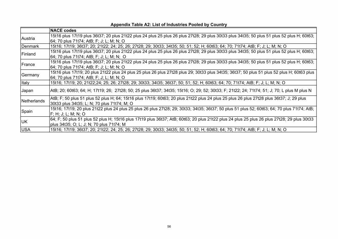
NACE codes

Austria 15t16 plus 17t19 plus 36t37; 20 plus 21t22 plus 24 plus 25 plus 26 plus 27t28; 29 plus 30t33 plus 34t35; 50 plus 51 plus 52 plus H; 60t63; 64; 70 plus 71t74; AtB; F; J; L; M; N; O

Denmark 15t16; 17t19; 36t37; 20; 21t22; 24; 25; 26; 27t28; 29; 30t33; 34t35; 50; 51; 52; H; 60t63; 64; 70; 71t74; AtB; F; J; L; M; N; O

Finland 15t16 plus 17t19 plus 36t37; 20 plus 21t22 plus 24 plus 25 plus 26 plus 27t28; 29 plus 30t33 plus 34t35; 50 plus 51 plus 52 plus H; 60t63; 64; 70 plus 71t74; AtB; F; J; L; M; N; O

France 15t16 plus 17t19 plus 36t37; 20 plus 21t22 plus 24 plus 25 plus 26 plus 27t28; 29 plus 30t33 plus 34t35; 50 plus 51 plus 52 plus H; 60t63; 64; 70 plus 71t74; AtB; F; J; L; M; N; O

Germany 15t16 plus 17t19; 20 plus 21t22 plus 24 plus 25 plus 26 plus 27t28 plus 29; 30t33 plus 34t35; 36t37; 50 plus 51 plus 52 plus H; 60t63 plus 64; 70 plus 71t74; AtB; F; J; L; M; N; O

Italy 15t16; 17t19; 20; 21t22;24; 25; 26; 27t28; 29; 30t33; 34t35; 36t37; 50; 51; 52; H; 60t63; 64; 70; 71t74; AtB; F; J; L; M; N; O

Japan AtB; 20; 60t63; 64; H; 17t19; 26; 27t28; 50; 25 plus 36t37; 34t35; 15t16; O; 29; 52; 30t33; F; 21t22; 24; 71t74; 51; J; 70; L plus M plus N

Netherlands AtB; F; 50 plus 51 plus 52 plus H; 64; 15t16 plus 17t19; 60t63; 20 plus 21t22 plus 24 plus 25 plus 26 plus 27t28 plus 36t37; J; 29 plus 30t33 plus 34t35; L; N; 70 plus 71t74; M; O

Spain 15t16; 17t19; 20 plus 21t22 plus 24 plus 25 plus 26 plus 27t28; 29; 30t33; 34t35; 36t37; 50 plus 51 plus 52; 60t63; 64; 70 plus 71t74; AtB; F; H; J; L; M; N; O

UK 64; F; 50 plus 51 plus 52 plus H; 15t16 plus 17t19 plus 36t37; AtB; 60t63; 20 plus 21t22 plus 24 plus 25 plus 26 plus 27t28; 29 plus 30t33 plus 34t35; O; L; J; N; 70 plus 71t74; M

USA 15t16; 17t19; 36t37; 20; 21t22; 24; 25; 26; 27t28; 29; 30t33; 34t35; 50; 51; 52; H; 60t63; 64; 70; 71t74; AtB; F; J; L; M; N; O

Appendix Table A2: List of Industries Pooled by Country

56

(1) (2) (3) (4) (5) (6) (7) (8) (9) (10) (11) (12) (13) (14) (15) (16) (17) (18)

∆ ((Imports+ Exports) / (Value Added)) 0.59 0.11

(0.15) (0.25)

∆ ((Imports) / (Value Added)) 1.07 0.21

(0.30) (0.45)

∆ ((Exports) / (Value Added)) 1.16 0.21

(0.30) (0.54)

∆ ((Imports OECD+ Exports OECD) / (Value Added)) 0.68 -0.05

(0.18) (0.37)

∆ ((Imports OECD) / (Value Added)) 1.44 -0.43

(0.52) (0.91)

∆ ((Exports OECD) / (Value Added)) 1.10 0.03

(0.30) (0.61)

∆ ((Imports+Exports nonOECD) / (Value Added)) 2.21 1.38

(0.58) (0.74)

∆ ((Imports nonOECD) / (Value Added)) 2.09 1.13

(0.63) (0.84)

∆ ((Exports nonOECD) / (Value Added)) 10.97 9.30

(3.38) (3.41)

∆ ((ICT capital) / (Value Added)) 107.61 73.59 107.29 73.22 110.10 74.17 109.89 76.18 110.56 78.66 112.20 75.32 110.15 69.78 113.49 71.75 116.71 67.65

(31.70) (31.41) (31.52) (31.32) (32.04) (31.41) (31.93) (31.56) (31.53) (31.36) (32.52) (31.53) (31.15) (30.48) (32.09) (30.78) (29.66) (29.74)

∆ ln(Value Added) 4.09 2.57 4.30 2.62 3.80 2.50 3.94 2.29 4.08 2.01 3.74 2.38 4.28 3.07 4.16 2.86 3.76 3.04

(1.09) (1.52) (1.13) (1.52) (1.06) (1.49) (1.09) (1.50) (1.11) (1.41) (1.07) (1.48) (1.12) (1.47) (1.16) (1.50) (0.97) (1.18)

∆ ((Non ICT capital) / (Value Added)) -0.63 0.97 -0.50 0.99 -0.76 0.95 -0.47 1.04 -0.01 0.91 -0.82 1.01 -1.09 0.62 -1.19 0.48 0.24 2.77

(2.41) (3.12) (2.38) (3.11) (2.45) (3.13) (2.39) (3.05) (2.33) (2.98) (2.46) (3.13) (2.50) (3.22) (2.51) (3.24) (2.42) (2.97)

1980 ( Research and Development Expenditure/ Value Added) 28.04 28.05 28.27 30.88 32.93 29.83 25.37 26.73 25.85

(17.59) (16.88) (18.06) (18.25) (17.32) (18.33) (15.55) (15.90) (13.84)

Country fixed effects X X X X X X X X X X X X X X X X X X

Obs. 84 65 84 65 84 65 84 65 84 65 84 65 84 65 84 65 84 65

R-squared 0.821 0.82 0.821 0.82 0.82 0.82 0.819 0.82 0.819 0.82 0.817 0.82 0.822 0.826 0.817 0.823 0.826 0.834

Appendix Table A3: Trade, ICT, and Research and Development

Dependent variable: High-Skilled Wage Bill Share

Notes: Coefficients estimated by OLS with robust standard errors in parentheses. Regressions weighted by the industry's 1980 share of each country's employment, for traded goods. The OECD ANBERD dataset does not have R&D data for

Austria and Spain, which are dropped from the sample (columns 2,4,6,8,10,12,14,16 and 18).

57

(1) (2) (3) (4) (5) (6)

Sectors All All Traded Traded All All

Method No Controls, OLS Full Controls, OLS No Controls, OLS Full Controls, OLS No controls, IV Full controls, IV

∆ (High-skilled wage-bill share) 10.02 10.02 9.37 9.37 10.02 10.02

∆ ((ICT capital) / (Value Added)) 0.018 0.018 0.017 0.017 0.018 0.018

Coefficient on ICT 72.3 46.9 83.1 75.5 152.3 121.6

Mean*Coefficient of ICT 1.32 0.86 1.45 1.31 2.78 2.22

Mean contribution % of ICT 13.16 8.54 15.43 14.03 27.72 22.14

Table and columns used Table 5 column (2) Table 5 column (4) Table 8 column (7) Table 6 column (6)

Research and Development/Value Added 0.028 0.028

Coefficient on R&D 52.79 30.08

Mean*Coefficient on R&D 1.49 0.84

Mean contribution of R&D 15.90 8.99

Appendix Table A4: Contribution of Changes in ICT and R&D to Changes in the High-Skilled Wage Bill Share

Notes: This table contains a "back of the envelope" calculation of the contribution of technology to accounting for the changes in the high-skilled wage bill share.

58

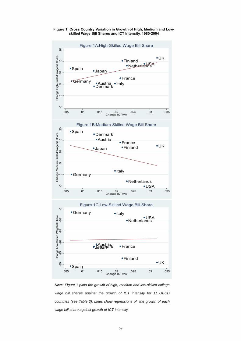
Figure 1: Cross Country Variation in Growth of High, Medium and Low-skilled Wage Bill Shares and ICT Intensity, 1980-2004

AustriaDenmark

Finland

FranceGermany Italy

JapanNetherlands

Spain

UKUSA

-50

510

1520

Cha

nge

Hig

h-S

kille

d W

ageb

ill S

hare

.005 .01 .015 .02 .025 .03 .035Change ICT/VA

Figure 1A:High-Skilled Wage Bill Share

AustriaDenmark

FinlandFrance

GermanyItaly

Japan

Netherlands

Spain

UK

USA-50

510

1520

Cha

nge

Med

ium

-Ski

lled

Wag

ebill

Sha

re

.005 .01 .015 .02 .025 .03 .035Change ICT/VA

Figure 1B:Medium-Skilled Wage Bill Share

AustriaDenmark

Finland

France

Germany Italy

Japan

Netherlands

SpainUK

USA

-30

-25

-20

-15

-10

-5C

hang

e Lo

w-S

kille

d W

ageb

ill S

hare

.005 .01 .015 .02 .025 .03 .035Change ICT/VA

Figure 1C:Low-Skilled Wage Bill Share

Note: Figure 1 plots the growth of high, medium and low-skilled college

wage bill shares against the growth of ICT intensity for 11 OECD

countries (see Table 3). Lines show regressions of the growth of each

wage bill share against growth of ICT intensity.

59

Figure 2: Average Annual Percentage Point Changes in High, Medium and Low-Skilled Wage Bill Shares over Six-Year Intervals from 1980-

2004 (Eleven Country Average and US)

-1-.5

0.5

1

Ave

rage

Ann

ualis

ed S

ix-Y

ear D

iffer

ence

in W

ageb

ill S

hare

1986 1992 1998 2004End Year of Six Year Interval

High MediumLow

Figure 2A: 11 Country Average-1

-.50

.51

Aver

age

Ann

ualis

ed S

ix-Y

ear D

iffer

ence

in W

ageb

ill S

hare

1986 1992 1998 2004End Year of Six Year Interval

High MediumLow

Figure 2B: USA Average

Note: Figure 2 shows annualised six-year average growth rates of high,

medium and low-skilled wage bill shares from 1980-2004, weighted by

employment share in the starting year of the six-year interval (e.g. The

1980-1986 annualised difference is weighted by each industry’s share in

the 1980 employment of the country).

60

Figure 3: Cross-Industry Variation in Growth of High-Skilled Wage-Bill Share and ICT Intensity, 1980-2004 (11 Country Means)

Agri

FoodTextilesWoodPaper

Chemicals

RubberMineralsMetals

MachineryElectrical

Transport

ManufacturingSale_motorWholesale

RetailTransport

Post

Real estate

Renting

Construction

Hotels

Financial

PublicEduHealthCommunity

05

1015

2025

3035

Cha

nge

Hig

h-Sk

illed

Wag

ebill

Sha

re

0 .05 .1Change ICT/VA

Figure 3A:Growth of High-Skilled ShareWhole Economy and Nontraded Industries

Agri

FoodTextilesWood

Paper

Chemicals

RubberMineralsMetals

Machinery

Electrical

Transport

Manufacturing

05

1015

20C

hang

e H

igh-

Ski

lled

Wag

ebill

Sha

re

0 .01 .02 .03 .04Change ICT/VA

Figure 3B: Growth of High-Skilled ShareTraded Industries Only

Note: Figure 3A plots the growth from 1980-2004 of high-skilled wage bill

shares against the growth of ICT intensity (ICT/VA), by industry, averaged

across countries. Lines show fitted values from regressions weighted by the

cross-country average of each industry’s share in 1980 employment (solid

line for entire economy, dashed line for non-traded industries only). Figure 3B

restricts the sample to traded industries.

61

Figure 4: Cross-Industry Variation in Growth of Medium-Skilled Wage-Bill Share and ICT Intensity, 1980-2004 (11 Country Means)

Note: Figure 4A plots the growth from 1980-2004 of medium-skilled wage bill

shares against the growth of ICT intensity (ICT/VA), by industry, averaged

across countries. Lines show fitted values from regressions weighted by the

cross-country average of each industry’s share in 1980 employment (solid

line for entire economy, dashed line for non-traded industries only). Figure 4B

restricts the sample to traded industries.

Agri

FoodTextilesWood

PaperChemicals

RubberMinerals

Metals

MachineryElectrical

Transport

Manufacturing

Sale_motorWholesale

Retail

Transport

Post

Real estate

Renting

Construction

Hotels

Financial

Public

Edu

Health

Community

-10

-50

510

1520

25C

hang

e M

ediu

m-S

kille

d W

ageb

ill S

hare

0 .05 .1Change ICT/VA

Figure 4A:Growth of Medium-Skilled ShareWhole Economy and Nontraded Industries

Agri

FoodTextiles

Wood

Paper

Chemicals

RubberMinerals

Metals

Machinery

Electrical

Transport

Manufacturing

510

1520

25C

hang

e M

ediu

m-S

kille

d W

ageb

ill S

hare

0 .01 .02 .03 .04Change ICT/VA

Figure 4B:Growth of Medium-Skilled ShareTraded Industries Only

62

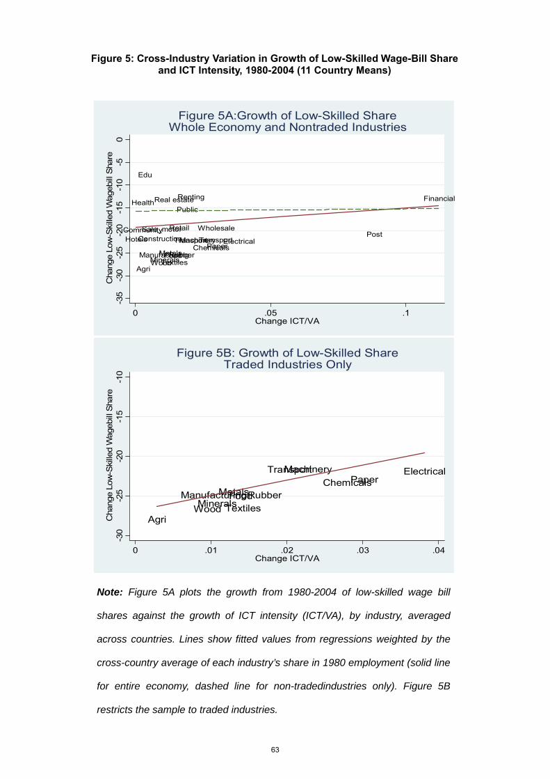
Figure 5: Cross-Industry Variation in Growth of Low-Skilled Wage-Bill Share and ICT Intensity, 1980-2004 (11 Country Means)

Agri

FoodTextilesWood

PaperChemicalsRubber

MineralsMetals

Machinery ElectricalTransport

Manufacturing

Sale_motor WholesaleRetail

TransportPost

Real estateRenting

ConstructionHotels

FinancialPublic

Edu

Health

Community

-35

-30

-25

-20

-15

-10

-50

Cha

nge

Low

-Ski

lled

Wag

ebill

Sha

re

0 .05 .1Change ICT/VA

Figure 5A:Growth of Low-Skilled ShareWhole Economy and Nontraded Industries

Agri

FoodTextilesWood

PaperChemicalsRubber

MineralsMetals

Machinery ElectricalTransport

Manufacturing

-30

-25

-20

-15

-10

Cha

nge

Low

-Ski

lled

Wag

ebill

Sha

re

0 .01 .02 .03 .04Change ICT/VA

Figure 5B: Growth of Low-Skilled ShareTraded Industries Only

Note: Figure 5A plots the growth from 1980-2004 of low-skilled wage bill

shares against the growth of ICT intensity (ICT/VA), by industry, averaged

across countries. Lines show fitted values from regressions weighted by the

cross-country average of each industry’s share in 1980 employment (solid line

for entire economy, dashed line for non-tradedindustries only). Figure 5B

restricts the sample to traded industries.

63