DEVELOPMENT OF A SOLAR SMOLENIEC/STIRLING HYBRID THERMO-MECHANICAL GENERATOR

FINAL TECHNICAL REPORT

Principal Investigator: Louise F. Goldberg, Ph.D (Eng)

Energy Systems Design Program Dept. of Biobased and Bioproducts Engineering University of Minnesota.

Sponsor: Initiative for Renewable Energy and the Environment

Institute on the Environment, University of Minnesota.

Project No.: RS-0014-11 Date: September 29, 2011 Revision: A.1

ACKNOWLEDGEMENT AND CERTIFICATION The research described herein has been performed with funding provided by the Initiative for Renewable Energy and the Environment. While this financial support is gratefully acknowledged, the Principal Investigator assumes complete responsibility for the contents herein.

STATEMENT OF CONFIDENTIALITY THIS REPORT HAS BEEN REDACTED SO AS NOT TO DISCLOSE CONFIDENTIAL UNIVERSITY OF MINNESOTA INTELLECTUAL PROPERTY REPORTED TO THE OFFICE OF TECHNOLOGY COMMERCIALIZATION UNDER DOCKET NO. ROI20100120. PLEASE CONTACT THE OFFICE OF TECHNOLOGY COMMERCIALIZATION (umotc@umn.edu) FOR FURTHER INFORMATION.

ii

ABSTRACT1 A closed-form state space analysis and a continuum mechanics simulation of the Solar Smoleniec/Stirling Hybrid Thermo-Mechanical Generator (SSH-TMG) invented at the University of Minnesota have been performed. These analyses produced an optimized functional prototype engine design with an electrical output power of 240 W at a net efficiency of 30% with a solar radiation heat input of 800 W. There is ample scope to scale-up the prototype design two- or three-fold to realize a target electrical output of about 1800 W. The achieved performance is competitive with a recently announced commercial high performance photovoltaic panel rated at 225 W at a module efficiency of 17.8 %.

1 The abstract has been written so that it is suitable for public dissemination.

iii

TABLE OF CONTENTS

ABSTRACT ................................................................................................................................ II

LIST OF TABLES ..................................................................................................................... IV

LIST OF FIGURES .................................................................................................................... V

NOMENCLATURE ................................................................................................................... VI

1. INTRODUCTION ................................................................................................................ 1

2. STATE SPACE ANALYSIS ............................................................................................... 2

2.1 BASELINE ENGINE DESCRIPTION ......................................................................... 2

2.2 BASELINE ENGINE OPERATION ............................................................................. 4

2.3 STATE SPACE ANALYSIS ........................................................................................ 6

2.4 STATE SPACE ANALYSIS SOLUTION ALGORITHM ............................................. 21

2.5 STATE SPACE ANALYSIS RESULTS .................................................................... 22

2.6 CLOSURE ............................................................................................................... 38

3. SIMULATION ANALYSIS ................................................................................................ 38

3.1 SIMULATION EQUATIONS ..................................................................................... 39

3.2 NUMERICAL SOLUTION METHODOLOGY ............................................................ 42

3.3 SIMULATION ANALYSIS RESULTS ....................................................................... 45

4 SIMULATION PROTOTYPE DESIGN .............................................................................. 52

5. CONCLUSION ................................................................................................................. 55

6 PROGNOSIS ................................................................................................................... 56

REFERENCES ......................................................................................................................... 56

iv

LIST OF TABLES Table 2.1 Baseline optimized SSH-TMG design ....................................................................... 24

Table 2.2 Results of optimization procedure ............................................................................ 25

Table 3.1 Simulation results for optimized SSH-TMG parameter set ........................................ 46

Table 3.2 Solar power variation for optimized SSH-TMG parameter set................................... 46

v

LIST OF FIGURES Figure 1.1 Thermo-Mechanical Generator ............................................................................... 1

Figure 2.1 Baseline SSH-TMG ................................................................................................ 3

Figure 2.2 Mounting frame ....................................................................................................... 5

Figure 2.3 State space analysis symbolic references ............................................................... 7

Figure 2.4 Alternator circuit .................................................................................................... 13

Figure 2.5 Cooler temperature optimization: parametric variation .......................................... 25

Figure 2.6 Cooler temperature optimization: performance at maximum power ....................... 26

Figure 2.7 Heater temperature optimization: parametric variation .......................................... 27

Figure 2.8 Heater temperature optimization: performance at maximum power ...................... 28

Figure 2.9 Displacer mass optimization: parametric variation ................................................ 29

Figure 2.10 Displacer mass optimization: performance at maximum power ............................. 30

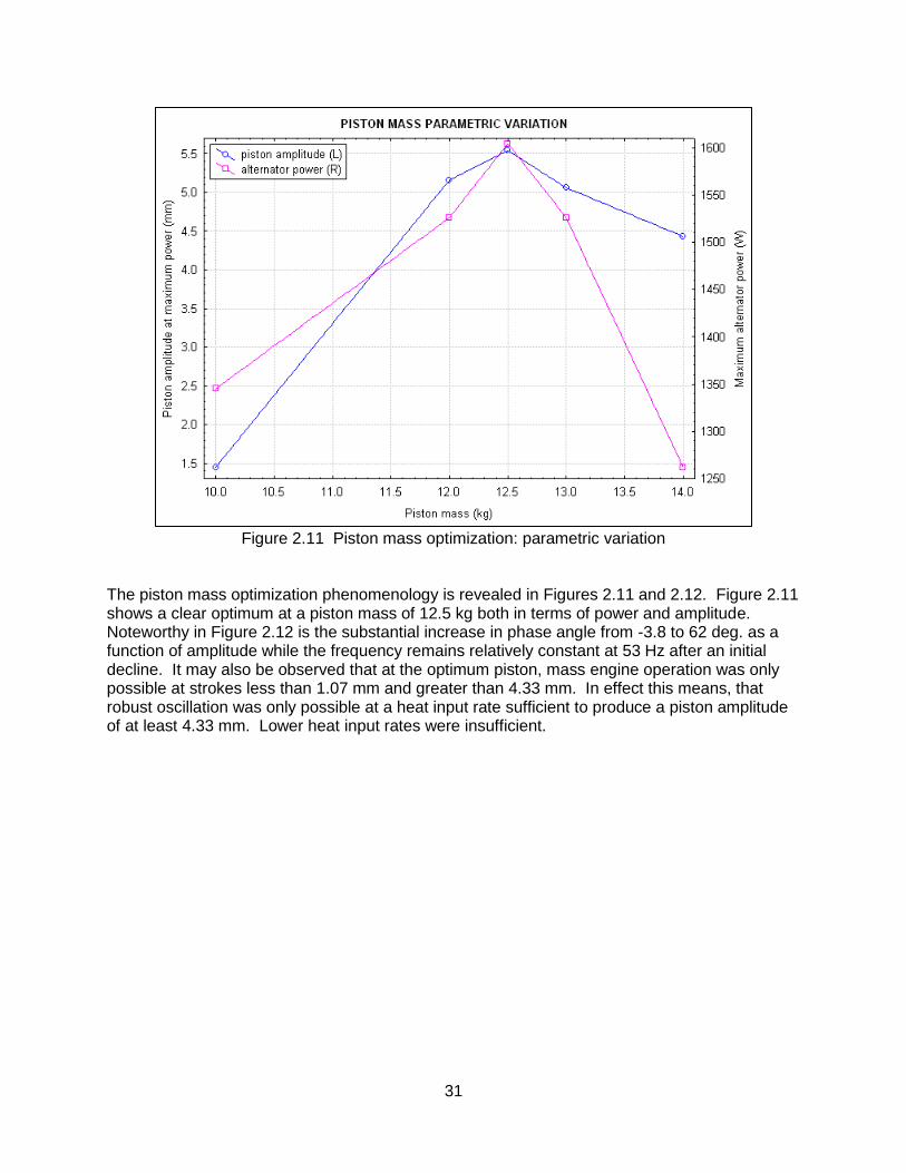
Figure 2.11 Piston mass optimization: parametric variation ..................................................... 31

Figure 2.12 Piston mass optimization: performance at maximum power .................................. 32

Figure 2.13 Casing mass optimization: parametric variation .................................................... 33

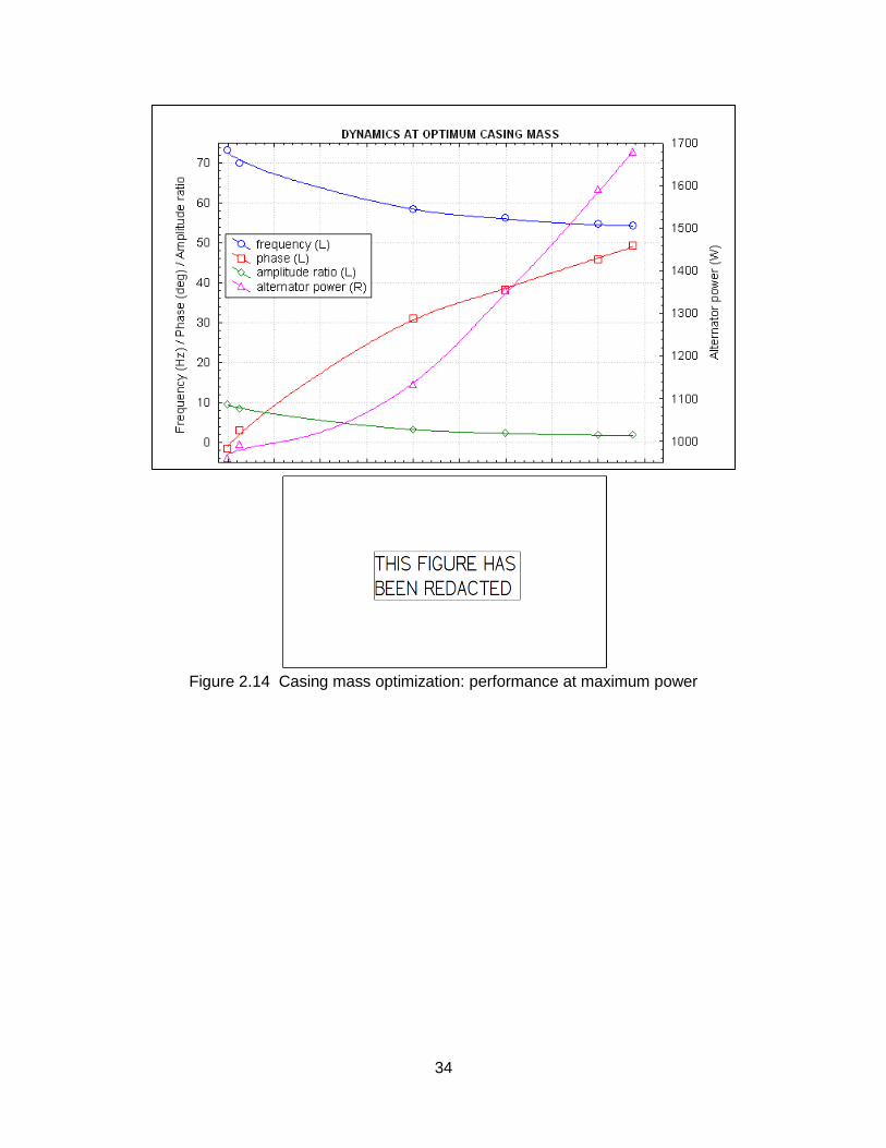
Figure 2.14 Casing mass optimization: performance at maximum power................................. 34

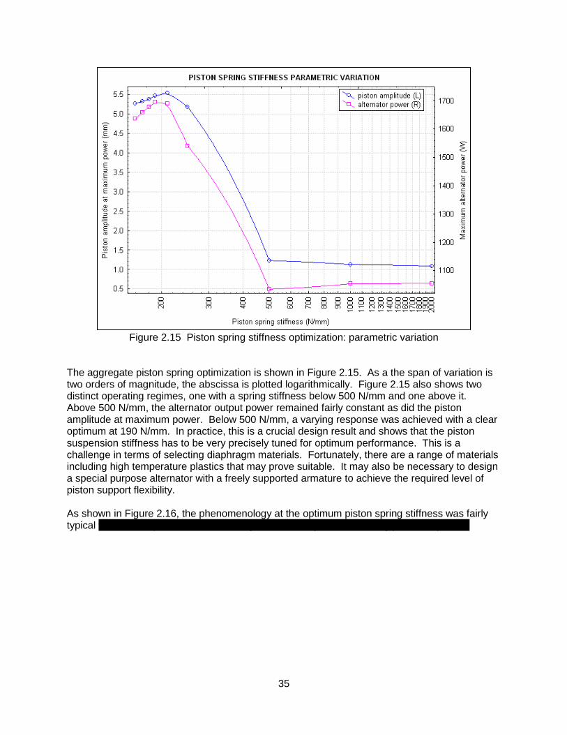
Figure 2.15 Piston spring stiffness optimization: parametric variation ...................................... 35

Figure 2.16 Piston spring stiffness optimization: performance at maximum power ................... 36

Figure 2.17 Compression space displacer clearance optimization: parametric variation .......... 37

Figure 2.18 Compression space displacer clearance optimization: performance at maximum

power .................................................................................................................... 38

Figure 3.1 Implementation of discretized equations ................................................................. 43

Figure 3.2 Aggregate piston spring stiffness variation phemonenology .................................... 47

Figure 3.3 Displacement temporal profiles at maximum efficiency ........................................... 49

Figure 3.4 Velocity temporal profiles at maximum efficiency .................................................... 50

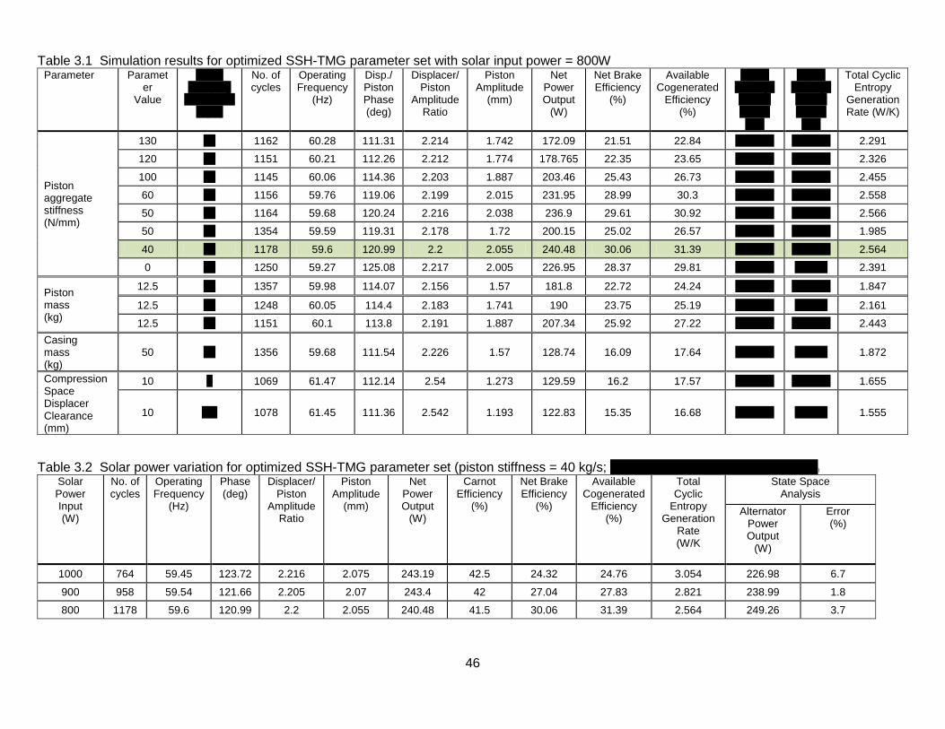
Figure 3.5 Pressure temporal profiles at maximum efficiency ................................................... 51

Figure 3.6 SSH-TMG overall final design ................................................................................. 53

Figure 3.7 SSH-TMG overall final design working space detail ................................................ 54

vi

NOMENCLATURE Bold Roman B state space coefficient matrix (components represented as and combined as )

E state space constant matrix (components represented as ) f external and mutual force vector g mass flux vector n unit normal vector q contact heat flux vector T extra stress tensor v velocity vector z state space vector (components represented as ) Italicized Roman A area (m2)

a real part of complex number b imaginary part of complex number

C heat capacity (J/kg.K) D diameter (m)

E external and mutual energy (J) volumetric flow rate (m3/s)

F Force (N) f frequency (Hz) K general constant

k stiffness (N/m) L length (m)

M mass (kg) P pressure (Pa)

Q heat (J) R gas constant (J/kg.K)

r displacer/piston amplitude ratio S entropy (J/K)

T temperature (K) t time (s)

V volume (m3) W work (J)

power (W) v velocity X amplitude (m)

x displacement (m) velocity (m/s)

acceleration (m/s2) Roman (used for electrical/magnetic symbols only)

B magnetic field strength (T) C capacitance (F) E potential (V)

I current (A)

current rate (A/s)

vii

L inductance (H) N no. of winding turns(

R resistance (ohm) Greek α mass ratio γ polytropic constant

θ phase angle (rad) κ engine thermodynamic constant (m3/K)

Λ pressure coefficient (kg/m2.s2) friction factor

density (kg/m3) magnetic flux (Wb)

angle (rad) general constant

ω angular velocity (rad/s) Subscripts a alternator ad alternator displacement

av alternator velocity ai alternator inner winding

ao alternator outer winding B bounce space

C compression space Cd compression space displacer clearance

E expansion space H heater

h hydraulic K cooler R regenerator d displacer

L load m displacer motor md motor displacement

mo motor offset mv motor velocity

n natural (0) previous time step

P at constant pressure p piston

ps piston support s casing

(s) system of particles ¨ second temporal derivative

T total (aggregate of expansion space, compression space, heater, regenerator and cooler) V at constant volume W working space

viii

generic Superscripts and Diacritical Marks

(t) turbulent ˙ first temporal derivative ^ per unit mass Operators d total derivative

partial derivative

inverse Laplace transform

time average of

volume average of

time average of volume average of

1

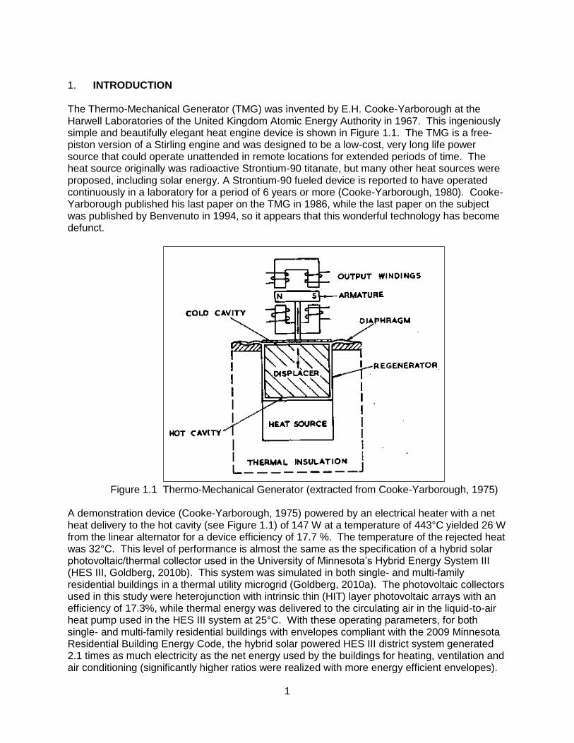
1. INTRODUCTION The Thermo-Mechanical Generator (TMG) was invented by E.H. Cooke-Yarborough at the Harwell Laboratories of the United Kingdom Atomic Energy Authority in 1967. This ingeniously simple and beautifully elegant heat engine device is shown in Figure 1.1. The TMG is a free-piston version of a Stirling engine and was designed to be a low-cost, very long life power source that could operate unattended in remote locations for extended periods of time. The heat source originally was radioactive Strontium-90 titanate, but many other heat sources were proposed, including solar energy. A Strontium-90 fueled device is reported to have operated continuously in a laboratory for a period of 6 years or more (Cooke-Yarborough, 1980). Cooke-Yarborough published his last paper on the TMG in 1986, while the last paper on the subject was published by Benvenuto in 1994, so it appears that this wonderful technology has become defunct.

Figure 1.1 Thermo-Mechanical Generator (extracted from Cooke-Yarborough, 1975)

A demonstration device (Cooke-Yarborough, 1975) powered by an electrical heater with a net heat delivery to the hot cavity (see Figure 1.1) of 147 W at a temperature of 443°C yielded 26 W from the linear alternator for a device efficiency of 17.7 %. The temperature of the rejected heat was 32°C. This level of performance is almost the same as the specification of a hybrid solar photovoltaic/thermal collector used in the University of Minnesota’s Hybrid Energy System III (HES III, Goldberg, 2010b). This system was simulated in both single- and multi-family residential buildings in a thermal utility microgrid (Goldberg, 2010a). The photovoltaic collectors used in this study were heterojunction with intrinsic thin (HIT) layer photovoltaic arrays with an efficiency of 17.3%, while thermal energy was delivered to the circulating air in the liquid-to-air heat pump used in the HES III system at 25°C. With these operating parameters, for both single- and multi-family residential buildings with envelopes compliant with the 2009 Minnesota Residential Building Energy Code, the hybrid solar powered HES III district system generated 2.1 times as much electricity as the net energy used by the buildings for heating, ventilation and air conditioning (significantly higher ratios were realized with more energy efficient envelopes).

2

The problem with realizing this level of net-zero energy performance in practice is the extremely high capital cost of a conventional hybrid solar collector with the described performance thus making its commercial deployment very difficult. Currently HIT PV arrays cost about $5000/kW while the thermal component adds $1000-2000 per thermal kW, for an aggregated cost of about $6500/kW for a commercially available system (Sundrum, 2010). This cost problem can be very neatly solved by deployment of a solar powered TMG as an alternative to the hybrid solar collector. Because of its extreme simplicity, absence of complex parts or fabrication techniques and use of standard engineering materials, it is expected that the device can be built on a mass-production basis for a cost of $1000 to 2000 / cogenerated kW, at least a three-fold reduction in cost of current hybrid PV/thermal collectors, so meeting current US Department of Energy goals. However, the TMG as shown in Figure 1.1 is very far from optimized and is not directly suitable for solar powered applications. The Principle Investigator (PI) has invented a completely revised version of the TMG based on extensive previous research with resonant-mode free-piston Stirling engines with both solid and liquid displacers (Goldberg, 1979, 1980, 1983, 1987a). While the original TMG operated on a nominal Stirling heat engine cycle, the revised engine operates on a generalized digital thermodynamic cycle named in honor of the late Prof. S. Smoleniec2. Thus when applied to a conventional Stirling cycle, the modified cycle may be referred to as a Smoleniec/Stirling cycle. The revised engine also addresses problems with the original TMG such as large conduction losses, poor heat transfer and regeneration and low working pressure while retaining the advantages of an intrinsically sealed containment pressure vessel and no dynamic seals. Hence the revised engine will be referred to henceforward as the SSH-TMG, or Smoleniec/Stirling Hybrid Thermo-Mechanical Generator. This project thus had the objective of developing, evaluating and optimizing the performance by closed form analysis and computer simulation of the SSH-TMG. The report is presented in three thematic sections. The first section describes an idealized closed-form analysis of the engine that was used to establish its basic operating parameters and, indeed, to determine whether it would operate at all. The second section discusses the development of a continuum mechanics analysis of the engine and its translation into a computer simulation that enabled a virtual engine to be tested experimentally. The final section reports some of the results and insights obtained from the simulation tests. 2. STATE SPACE ANALYSIS 2.1 BASELINE ENGINE DESCRIPTION The baseline engine is described with reference to Figure 2.1. A lower metal and upper ceramic casing are mechanically fastened together to create working and bounce spaces separated by the piston diaphragm. The bounce space contains the power linear alternator that is supported on a spring to balance its weight. The linear alternator has a fixed armature coil attached to the lower plate of the bounce space and a moving permanent magnet attached to the central section of the piston diaphragm. The mass of the permanent magnet is adjusted to tune the resonant oscillating frequency of the piston assembly.

2 Prof. Smoleniec was a beloved teacher and later friend of the PI during her years as an undergraduate

and graduate student at the University of the Witwatersrand. He suggested the outline of the basic concept behind the Smoleniec cycle to the PI during a coffee break during one of our joint consulting projects.

3

The working space consists of the thermodynamically active region (termed the working space) containing, from the top of the engine: the expansion space; heater; regenerator; cooler; and, compression space. As the average cyclic pressures in the working and bounce spaces are constrained to be equal, the net pressure difference across the piston diaphragm is small and thus its flexible elements can be manufactured from a flexible high-temperature polymer to obtain an optimum low stiffness.

Figure 2.1 Baseline SSH-TMG

The displacer is attached to the casing by upper and lower support diaphragms whose flexible elements are metallic so they can withstand elevated gas temperatures as well as achieve the higher degrees of stiffness desirable for the net displacer spring constant. The casing is sprung to ground so that it can oscillate freely in the vertical plane. In the baseline configuration, the heater is represented as an annulus between a spirally grooved solid core and the wall of the displacer assembly tube. The solid core is mounted into the top ceramic plate at the focus of a Fresnel lens (see Figure 2.2). The cooler also is represented as an annulus between the wall of the displacer assembly tube and the coolant chamber. The coolant chamber is formed from a capped hollow tube with a central plug around which cooling water is circulated. The coolant chamber is supported by a four-legged spyder fabricated from small-diameter tubes (approximately 0.25 in. external diameter) that penetrate the lower casing wall. Two of the tubes provide the cooling water intake and two the cooling water exhaust. The regenerator is formed by a stack of woven mesh screens sandwiched between the heater and cooler. A minimal gap is maintained between the edge of the regenerator screen stack and the displacer tube inner wall to permit the displacer to oscillate freely. This gap also is considered as part of the regenerator. The metallic displacer tube itself is split into upper and lower sections that are joined by a ceramic sleeve with an internal spacer ring that thermally and electrically isolates the upper and lower sections. A metal annulus is attached to the upper section of the displacer tube and is sized to tune the resonant frequency of the displacer. The lower section supports a coil that forms the moving armature of a linear motor/alternator (depending on whether, effectively, power is supplied to the coil or a load is placed across it). The coil winding is insulated from the lower displacer tube by an appropriate insulator such as a sheet of mica. One end of the coil is attached to the upper displacer tube and the other to the lower displacer tube. The upper and lower displacer tubes are each connected to the upper and lower displacer metallic support diaphragms that in turn are attached to metallic elements of the upper and lower casing. Since

4

the upper and lower casings are separated by an electrically insulating ceramic tube, power to the displacer moving armature may be supplied by attaching wires to the metallic portions of the upper and lower casings. The displacer motor stator is formed by a toroidal permanent magnet mounted on the upper plate of the lower casing. This upper plate is penetrated by a series of holes that serve to equalize the pressure between the compression space and the displacer cavity. Note that the upper and lower displacer support diaphragms seal the displacer cavity from the expansion and compression spaces. Further, as the upper and lower displacer diaphragms are structurally identical and oscillate in phase, the volume of the displacer cavity is constant and thus, at engine equilibrium operating temperature, its pressure will be constant as well. As the pressure of the displacer cavity is initialized to be equal to the mean working space pressure, the pressure difference across the upper and lower displacer diaphragms will be constrained to be relatively small (compared with the initial engine pressurization) and equal to half the pressure drop between the expansion and compression spaces generated by the working fluid flow through the displacer tube (combined heater, regenerator and cooler pressure drops). Finally, an electronic controller generates a driving potential (voltage) across the displacer armature coil that produces either a motor or an alternator function. This voltage may have an arbitrary profile combining sinusoidal and/or square wave components generally represented by Fourier and Walsh series. The SSH-TMG is mounted in dual-axis solar tracking frame as shown in Figure 2.2. The frame consists of a top structure fabricated from welded H-section beams that generate a square mesh. Each cell of the mesh contains a single cell mounting shell attached to the supporting frame by damping blocks that absorb the oscillatory motion transferred from the SSH-TMG support springs. A square acrylic Fresnel lens is attached to the top of the mounting shell. As shown, the engine is positioned so that the optical focus of the Fresnel lens coincides with the top of the heater core. 2.2 BASELINE ENGINE OPERATION With reference to Figure 2.1, the displacer assembly, piston assembly and casing form a coupled spring/mass system whose natural resonant frequencies are given respectively by Equations 2.1.

√

√

√

5

Figure 2.2 Mounting frame (redacted)

Generally, the displacer mass Md is chosen to yield the basic engine operating frequency for a

given displacer spring stiffness kd. The piston and casing masses and spring stiffness are then set so that they are both slightly detuned from having the same natural frequency as the

displacer with the frequency differences fs – fd and fp – fd determining the critical phase difference between the displacer and piston oscillation that is necessary for the engine to produce positive power. As the displacer oscillates out of phase with the piston, the working fluid (gas) in the working space experiences a pseudo-Stirling cycle with the following four steps beginning with the displacer at top dead center and the piston moving upwards from its equilibrium position (the piston is assumed to be at the ideal 90° in phase behind the displacer for explanatory purposes):

As the displacer moves downwards, gas is transferred from the compression space progressively through the cooler, regenerator and heater. As the gas moves upwards, it is first cooled by the cooler releasing the heat of compression. Then it is progressively heated by heat stored in the regenerator followed by the heat transferred in the heater derived from the solar insolation impinging on the heater cap. As the gas is heated it increases in pressure, so increasing the overall engine working space pressure. In an ideal Stirling engine, this gas transfer occurs with the piston fixed and is thus isochoric (occurs at constant volume). In the actual engine the gas heating process is only approximately isochoric owing to the decelerating upwards motion of the piston.

When the displacer reaches its equilibrium position on its downwards travel, the piston reaches top dead center just as the working space pressure begins to exceed the cycle average pressure. Thus the piston is accelerated downwards by the increasing working space pressure until the displacer reaches its bottom dead center position. This constitutes the expansion stage of the cycle that, in an ideal Stirling cycle, is regarded as being isothermal. In the SSH-TMG, the expansion and compression

6

spaces are polytropic, that is, compression and expansion essentially occurs adiabatically with a small amount of forced convection heat transfer from their bounding walls.

As the piston passes the equilibrium position on its downward stroke, the displacer begins to move upwards, transferring the gas from the expansion space to the compression space through the heater, regenerator and cooler. As it passes through the heater, the gas is reheated so offsetting the decrease in temperature produced from the prior expansion phase. Thereafter, as the gas passes through the regenerator, it progressively transfers heat to the regenerator matrix which stores the heat for use in reheating the gas during the next cycle. The gas then passes through the cooler where it is further cooled to its minimum cycle temperature. As the gas is cooled, it decreases in pressure, so decreasing the overall engine pressure. Again in an ideal engine, this gas transfer occurs with the piston fixed producing an isochoric heat transfer. In reality, the gas cooling process is only approximately isochoric owing to the decelerating downwards motion of the piston.

When the displacer reaches its equilibrium position on its upwards stroke, the piston reaches bottom dead center just as the working space pressure decreases below the cycle mean pressure. As the piston moves upwards (driven by the stored energy in the springs as well as the compressed gas in the bounce space), it compresses the gas constituting the compression phase of the cycle. In an ideal Stirling cycle, the compression is isothermal, however, in the SSH-TMG, as noted above, it is polytropic. At the end of the compression phase, the piston is moving upwards at its equilibrium position and the displacer is at top dead center, center, so closing the cycle.

In the Smoleniec version of the pseudo-Stirling cycle, the displacer motion is dynamically retarded or accelerated by the displacer linear alternator/motor so that the displacer/piston phase is controlled throughout the cycle to optimize the performance. Many control strategies are possible such as optimum phase control (that tends to optimize the efficiency) in which the displacer is controlled to yield an average phase angle of 90°. Alternatively, the displacer can be controlled to maximize the alternator power output which generally yields an average displacer/piston phase angle in the 110 – 140° range. A more sophisticated control using an embedded algorithm to calculate the cyclic entropy generation rate as a function of displacer, piston and casing motion also is possible and this control generally yields the best compromise between power output and thermal efficiency. 2.3 STATE SPACE ANALYSIS The basic functionality of the SSH-TMG was determined by a closed-form solution of the governing dynamic equations using a state-space analysis technique developed by the author (Goldberg, 1987a). Variants of this technique developed by others also have informed the analysis particularly as applied to a traditional TMG (Benvenuto and de Monte, 1995a, 1995b). The analysis is performed with reference to the symbolic dimensions and motion referential positions and sign conventions shown in Figure 2.3.

7

Figure 2.3 State space analysis symbolic references

The dynamics of the displacer, piston and casing are given by:

( )( )

( )( )

Since is a function of the alternator current and rate of change of alternator current while , and are functions of , , , and , (2.2) through (2.4) yield 8 variables for

which the equations need to be solved. This will produce an 8th order characteristic equation that by the Abel-Ruffini3 theorem has no general algebraic solution. Thus it is necessary to reduce the number of variables to at most four for which a general closed-from solution can be obtained. In the first instance, it is possible to reduce the number of variables to 6 by eliminating the casing motion. Summing (2.2) through (2.4) yields:

Following Redlich and Berchowitz, 1985, the LHS inertial terms are much greater than the casing spring force (or the casing oscillation amplitude is much smaller than those of the piston and displacer) so the engine can be treated as a free body. Thus (2.5) yields:

( )

Thus the momentum of the entire engine is constant and since it is initially at rest, equal to zero. Thus (2.5) can be solved to yield a relationship between the displacements expressed in terms of mass ratios as:

where:

3 The Abel-Ruffini states that there is no general algebraic solution (that is, a solution in terms of radicals)

for polynomial equations of fifth or higher order.

8

⁄⁄

It should be noted that (as will be shown in Section 3) that (2.6) is has its limitations since although the casing motion is less than those of the displacer and piston, it is not relatively negligible, particularly at lower engine operating frequencies at which the optimum performance is obtained. Expressed differently, (2.6) necessarily yields a high frequency engine motion. (2.7) eliminates (2.4) and after substitution into (2.2) and (2.3) yields:

{ }

( ){ ( ) }

Before equations (2.9) and (2.10) can be solved, all the terms must be expressed in terms of

and and their temporal derivatives. Beginning with the thermodynamic terms, the pressure

difference represents the pressure drop across the displacer tube produced by friction as the gas flows through the heater, cooler and regenerator. Thus representing this pressure

difference as , following Benvenuto and de Monte, 1995b, it is assumed that: ⁄ ⁄ that yields the stipulated equality in (2.11) can be determined from the engine thermodynamics. In this analysis, it is assumed that the expansion, compression and bounce spaces are polytropic and that the heater, cooler and regenerator are isothermal. This is a more generalized approach than that adopted previously (Goldberg, 1983) in which the variable volume (or working) spaces were treated as adiabatic. In this case, heat transfer is allowed in the working spaces as well as required by the characteristics of the SSH-TMG. By substituting the perfect gas equation of state into the time differential of the

polytropic process equation (

)

, it can be shown that for the expansion, compression

and bounce spaces:

where the subscript takes on the values E, C or B. Noting that the volume of the heater and cooler (annulus between the core and the displacer tube ) have variable volumes, differentiating the perfect gas equation of state and noting that the temperature is isothermal yields:

(

)

where the subscript takes on the values H or K. Finally for the regenerator that is also isochoric:

9

where the regenerator temperature is represented by a log mean temperature (Creswick, 1965):

(

)

Assuming that the working and heat transfer spaces are hermetic (that is, no gas leakage occurs), the total mass of gas is constant, or: Differentiating, substituting (2.12), (2.13), (2.14) and rearranging yields the following

expression for :

κ(

)

where:

κ (

)

After substitution of (2.7), the volumes in (2.17) may be expressed as:

{ }

{ }

{ }

where represents the volumes at and while represents the gas flow

areas in the components referred to. Taking the time derivative of (2.19), substituting into (2.17) and collecting terms produces:

κ(

)

where:

κ

Substituting the time derivative of (2.19) into (2.20) and collecting terms:

10

κ[ { (

)

}

{ (

)

}]

Invoking a MacLaurin series to linearize yields:

and differentiating with respect to time:

Hence equating terms in (2.22) and (2.24) yields:

κ [ (

)

]

κ [ (

)

]

Thus (2.25) allow to be expressed entirely in terms of displacer and piston motions. Assuming that the bounce space also is polytropic and that it is hermetic (no gas leakage), a derivation similar to that for (2.12) yields:

Similar to (2.19), is given by:

( )

Substituting the time derivative of (2.27) into (2.26) and collecting terms:

[ ( )]

Linearizing using the same procedure as in (2.23) through (2.25) gives:

11

( )

Note that at rest, the SSH-TMG is uniformly pressurized so that . Thus (2.30) allow to be expressed entirely in terms of displacer and piston motions as well. The pressure drop across the displacer may be expressed as a function of the average volumetric flowrate through the displacer tube that may be expressed in terms of the expansion and compression space volumetric change rates by:

(

)

Substituting the derivatives of (2.19a,d) and collecting terms produces:

[ ( ) { }]

whence it follows that the flow velocities in the heater, regenerator and cooler are given by:

In this analysis, the following model for calculating the linearized displacer pressure drop

is adopted from purely physical arguments:

[

| |

|( )

|]

The first term on the RHS of (2.33a) is zero (since there is no pressure drop when the flow is zero), while the multiplicand of in the second term represents the maximum possible pressure drop per unit flow rate when the displacer and piston motions are sinusoidal as is the case in the SSH-TMG. Thus (2.33) yields the correct

phenomenology in that when is non-zero, the pressure drop experienced is linearly proportional to the maximum possible pressure drop, and when is zero, the pressure drop is zero as well. Define a friction factor in terms of the flow kinetic energy in the usual manner as (Bird, et al, 1960):

where denotes H,R or K. Noting that is the sum of the individual pressure drops in the heater, regenerator and cooler, substituting (2.31), (2.32) and (2.34) into (2.33), rearranging and collecting terms yields:

[( ) |( )

| { }| |] ∑(

)

[ ( ) { }]

12

Thus given that can be determined from standard friction factor correlations (Kays and London, 1964), (2.35) allows to be expressed in terms of

and . For convenience define:

[( ) |( )

|

{ }| |] ∑(

)

So that:

[ ( ) { }]

The force applied by the displacer linear motor/alternator can be expressed simply as the sum of offset, spring and damping forces as follows: The three constants and are used in the engine control system to optimize the engine performance Substituting (2.7) and collecting terms:

{ } { }

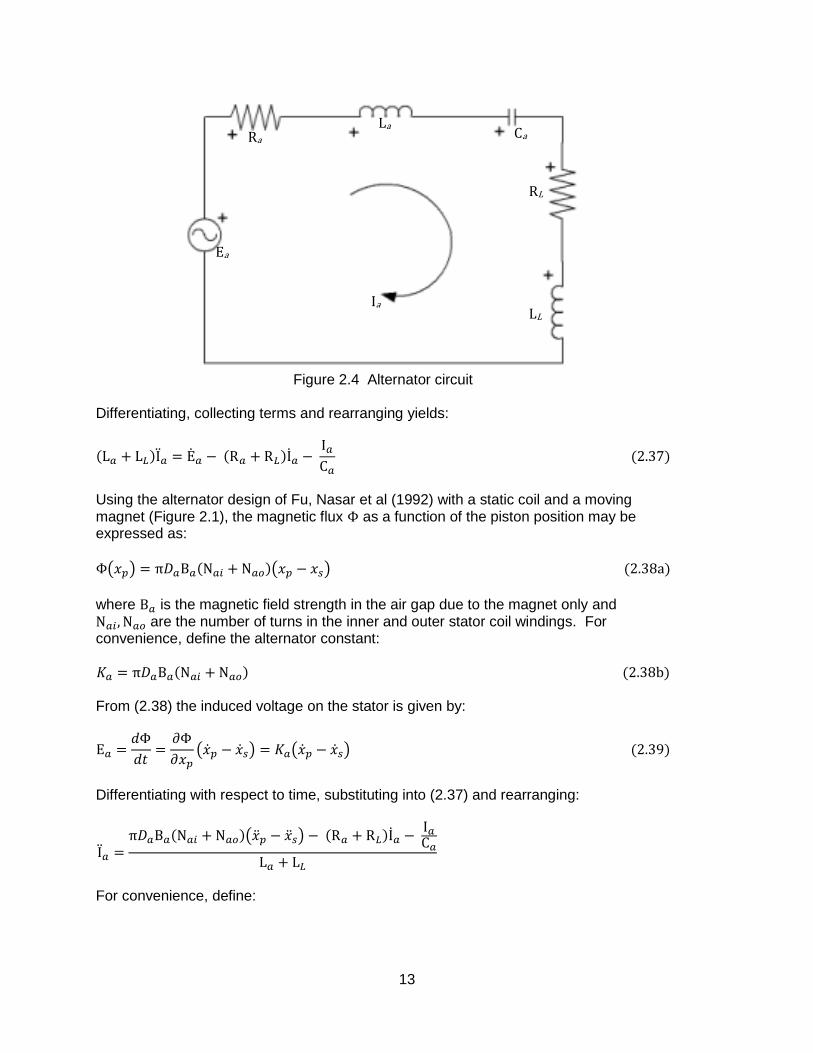
The force applied by the alternator can be resolved with respect to the circuit diagram shown in Figure 2.4. The alternator is depicted as an alternating voltage source, resistor

and inductor connected in series (with subscripts a) while the load is represented as a resistor and inductor in series (with subscripts L). In general, there are two approaches to depicting an alternator/load circuit. The series approach shown places the tuning capacitor Ca in series with the load, while in the alternate parallel approach, the tuning capacitor is placed in parallel with the load. For the sake of analytical simplicity, the series approach is adopted as it simplifies the analysis without any loss of generality. Applying Kirchoff’s law to Figure 2.4 (noting the sign convention depicted by the ‘+’ signs):

∫

13

Figure 2.4 Alternator circuit

Differentiating, collecting terms and rearranging yields:

Using the alternator design of Fu, Nasar et al (1992) with a static coil and a moving magnet (Figure 2.1), the magnetic flux as a function of the piston position may be expressed as:

( ) ( )

where is the magnetic field strength in the air gap due to the magnet only and are the number of turns in the inner and outer stator coil windings. For convenience, define the alternator constant: From (2.38) the induced voltage on the stator is given by:

( ) ( )

Differentiating with respect to time, substituting into (2.37) and rearranging:

( )

For convenience, define:

Ia

Ea

Ra

La Ca

RL

LL

14

Then substituting these constants as well as (2.7) yields:

{( ) }

Noting that by the conservation of energy, the rate of work done on the alternator by the piston is equal to the electrical energy generated, or:

( )

Substituting (2.39) and cancelling terms: Equation (2.40) is the third fundamental equation that together with (2.9) and (2.10) completely describe the SSH-TMG. However, as discussed previously, while these

three equations can be solved for the six variables , , , , and , a general

closed-form solution is not possible. Thus it is still necessary to eliminate at least two more variables. This can be accomplished by assuming that the current generated by the alternator is a function of the piston velocity and displacement only (Benvenuto et al, 1995a) which is reasonable when the engine is operating at steady state and the alternator loads are assumed to be linear. Further, previous analysis (Goldberg, 1987a), has rigorously demonstrated that any 4th order characteristic equation will only yield stable, steady-state free displacer and piston oscillations if the characteristic equation has one pair of complex conjugate eigenvalues with zero real parts and two negative real eigenvalues. In these circumstances, the oscillation of the piston and displacer and, from (2.7), the casing as well, will be sinusoidal4. Thus, define the steady-state displacer and piston displacements as follows:

For later convenience, define an amplitude ratio ⁄ , substituting and

differentiating twice with respect to time yields the following expressions for displacement, velocity and acceleration:

Thus per the above argument, noting that the absolute piston motions must be expressed relative to the displacer motions, define:

4 The validity of this reasoning is confirmed in Section 3 where the full set of equations are solved

numerically and the solution yields sinusoidally varying displacer, piston and casing motions.

15

( ) ( )

Substituting (2.7), then (2.42a,b) and rearranging:

{( ) }

{( ) }

Differentiating (2.44a) successively twice with respect to time yields:

{( ) }

{( ) }

{( ) }

{( ) }

Substituting (2.44) into (2.40b) and then equating the sine expression

{( ) } terms on the LH and RH sides yields:

Similarly, equating LHS and RHS terms for the cosine expression

{( ) } gives:

Finally, solving (2.45) simultaneously yields:

Substituting (2.7), (2.46) into (2.43) and substituting the result into (2.41b) yields the final result:

[ { ( ) } { ( ) }]

that expresses the alternator force on the piston entirely in terms of the piston and displacer motions. Substituting (2.36a), (2.35) and (2.11) into (2.9), simplifying and collecting terms yields:

16

{ ( )}

{ } (2.25), (2.23), (2.30) and (2.29) allow the pressure difference to be expressed as: Λ Λ

where:

Λ

[ (

)

]

Λ

κ [ (

)

]

( )

Then, from (2.11), the pressure difference across the piston diaphragm can be expressed as:

Λ Λ [ ( ) { }]

Substituting (2.50) and (2.47) into (2.10), simplifying and collecting terms:

{( )( ) Λ }

{ ( ) ( )}

{ ( ) Λ }

[ { }]

Define the state space vector as follows:

[

] [

]

(2.52), (2.51) and (2.48) can be expressed as the linear equation: where:

where the constants , and are derived from (2.51) and (2.48) so that (2.53) can be expressed as:

17

[

] [

] [

] [

]

By Laplace transformation, (2.53) has the solution:

{ }{ } The eigenvalues are determined from the characteristic equation: | | or:

|

|

After successive cofactor expansions, this yields the desired 4th order characteristic equation:

where:

As noted above, in order for the SSH-TMG to display stable oscillation, two of the roots of (2.57) must be complex conjugates. Thus choosing , substituting into (2.57) and equating real and imaginary parts with zero:

But, for stability, the real part must be zero (again noted previously), that is . Hence (2.58) gives:

whence from the imaginary part:

substituting into the real part and rearranging:

18

(2.59b) represents the “design” equation of the SSH-TMH, that is, the equality that must be satisfied by the engine parameters in order for stable oscillation to be achieved. Under these conditions, the operating angular velocity is given by the imaginary root , or:

√

Examining (2.42) shows that a solution for 4 variables is required, namely, and .

However, there are only 3 independent equations for the solution, namely, (2.48), (2.51) and (2.59b). The fourth equation is provided by the requirement for closing the overall engine energy balance as expressed by the first law of thermodynamics under steady-state conditions, or:

∮ ∮

However, as the heater and cooler are assumed to be isothermal, cannot be calculated

directly, or alternately, if is specified as a boundary condition (such as the insolation provided by the Fresnel lens), then the heater and cooler working fluid temperatures are indeterminate. However, following Goldberg (1987), it is self-evident that is solely dependent on the heat

added to and removed from the engine, thus treating as a parameter is equivalent to setting

the thermal energy supply boundary condition. Thus in this analysis, is treated as a

parameter. In order to make the solution of (2.59b) tractable, it was determined that the optimum approach was to treat all the parameters appearing in equations (2.48) and (2.51) as parameters with the

exception of the displacer motor damping coefficient that is treated as a variable that can be determined by satisfying (2.59b). Noting that from (2.54) and (2.48) appears in the coefficients and while from (2.57b)

these coefficients only appear in the constants and . Thus (2.59b) shows that the solution for can be expressed as a cubic polynomial that can be solved analytically using Cardano’s method (Nickalls, 1993, the algebraic manipulations are not material to the analysis and are thus omitted). For a given set of parameters, the motor stiffness coefficient is varied about a value of zero to establish the range of possible engine performance and the

maximum power output for that parameter set. In practice, would be used to tune the stiffness of the displacer suspension diaphragms, that is:

Thus given as a parameter and that the solution of (2.59b) for allows the determination

of from (2.59c), and can be determined by substituting (2.42) into (2.51). Thus in terms of the coefficients, this yields:

19

Equating the sine and cosine components separately with zero yields two equations that can be solved simultaneously to yield:

[

]

√

where:

Remaining to be determined are the mean expansion and compression space temperatures and in (2.25). Substituting the time differential of the perfect gas equation of

state ⁄ into the LHS of (2.12) and simplifying yields:

where takes on the values E, or C. Since the displacer and piston motions are sinusoidal, it follows that the maximum pressure and temperature differences and are likewise related to the correlated mean cyclic values at by

(2.64) so that:

Following Finkelstein (1960), the mean expansion and compression space temperatures may be expressed as: Substituting (2.66) into (2.65) and rearranging:

(

)

(

)

From (2.25) define:

[ (

)

]

20

[ (

)

]

Then substituting (2.25), (2.42b) and (2.68) into (2.24) and simplifying:

κ [ ]

where The maximum pressure occurs at when

. Hence

(2.69) yields:

[

]

and, because the displacer and piston motions are periodic with a periodicity of radians: Substituting (2.25), (2.42a) and (2.68) into (2.23) and simplifying:

κ [ ]

Now: Substituting (2.71) and a trigonometrical representation of (2.70), simplifying and rearranging yields:

κ √[( )

( )

]

Finally, substituting (2.72) into (2.67):

κ √[( )

( )

]

κ √[( )

( )

]

It can be observed that (2.73) are non-linear and transcendental because from (2.68) and (2.21) κ , and are all functions of and that in turn include trigonometric

functions. Thus, the equations need to be solved iteratively using the algorithm discussed in the next section. As the heater, regenerator and cooler are assumed to be isothermal, closed-form solutions for the external heat transfers are not tractable. Thus the calculation of the overall engine heat balance is postponed to the full gas dynamics simulation of the engine described in Section 3.

21

Thus the performance metric used is the alternator output power . From the derivation of (2.41), the cyclic net work done on the alternator by the piston is given by:

∮ ( )

Substituting (2.7) and (2.47):

∮{ ( ) }[ { ( ) } { ( ) }]

Substituting (2.42b), performing the necessary cyclic integrals, simplifying and rearranging yields:

[( )

( )

]

Hence the alternator output power is given by or:

[( )

( )

]

2.4 STATE SPACE ANALYSIS SOLUTION ALGORITHM The basic solution algorithm may be expressed using a prototypical programming language as: Basic Algorithm: Initialize { ;

;

( )

;

}

while ( | | ) {

find from appropriate friction factor correlations where is determined

by (2.31) and (2.32)

solve (2.59b) for ;

solve (2.59c) for ;

solve (2.62) for and ;

solve (2.73) for and ;

from (2.42b):

( )

;

22

;

}

solve for engine performance (2.77).

The phase angle is used as the metric of algorithm convergence. The engine performance can thus be optimized in terms of the Basic Algorithm as follows: Optimization Algorithm: Input engine parameters;

set ; find

and from (2.59b) by requiring that the solution yield a real root for

invoke the Basic Algorithm to find the maximum on the interval [ ] by

parabolic interpolation. These algorithms have been implemented in a computer program that allows the engine parameters to be tuned for maximum power output. The results of the analysis are discussed in section 2.5. 2.5 STATE SPACE ANALYSIS RESULTS During the course of the project, hundreds of different parameter combinations describing several different design configurations were investigated. For example, during the course of the simulation analysis, it was discovered that the pressure drop across the displacer tube was critical to achieving stable operation. Thus the original concept of a wire mesh regenerator screen stack proved unacceptable since it generated an excessive pressure drop. Hence it became necessary to replace the wire mesh regenerator with a tubular regenerator in order to significantly lower the pressure drop at the expense of regenerator effectiveness. Hence the base parameter set reported in Table 2.1 more or less represents the final design parameter set realized at the end of the simulation analysis. The alternator dimensional design is based on a commercial 5 kW unit manufactured by Q-Drive (Q-Drive, 2010, model no. 1S297M/A), while the magnetic and electrical properties are based on data presented by Kankam, et al (1992) and Fu and Rosswurm (1992) that were developed for conventional free piston Stirling engine linear alternators. The annular heater and cooler use fluted inner cores to promote increased heat exchange as described by Garimella and Christenson (1995a and b). As discussed in Section 2.4, all the results are presented parametrically as a function of piston amplitude. During the simulation, the maximum achievable piston amplitude with a solar input of 1kW is less than 5 mm. A practical limit on achievable piston amplitude is a function of the piston diaphragm and alternator rotor suspension stiffness that likely would not exceed 3 mm. Thus, for the purpose of the parametric performance investigation, each permutation is run up to a piston amplitude at which the displacer stroke is limited by the displacer clearance height in the expansion space. In this context, the baseline aggregate piston stiffness (diaphragm and alternator rotor suspension) reported in Table 2.1 is 179.69 N/mm which is the minimum (from

23

an early revision of the simulation5) that will permit a real solution to the engine design equation (2.59b). From Table 2.1, it is evident that in terms of the solution algorithm there are at least 56 parameters assuming that the regenerator, cooler and heater configurations are not changed and only helium is used as the working fluid. This would yield a parametric performance map requiring 8 x 1037 permutations that clearly is not tractable. During the course of the project during which multiple combinations of parameters were evaluated as well as from the experimental performance of the conventional TMG (Cooke-Yarborough 1975, 1980, 1985, 1986) the following reduced list of parameters was found to be critical

aggregate piston spring stiffness

heater temperature

cooler temperature

compression space displacer clearance height

displacer mass

piston mass

casing mass Thus the data presented below focus on the parametric variation of these 7 parameters. Each variation is parametric in the piston displacement as previously discussed while the displacer motor control variables (stiffness and damping coefficients) are the dependent variables. In this

context, the displacer motor offset constant was held constant at zero since it is not necessary to vary the displacer mean position in order to optimize the performance. For each parametric permutation, the results presented are the maximum alternator power output and the operating frequency, displacer phase angle and displacer/piston stroke ratio at the maximum power output. The optimization technique used is a variation of the “successive incremental optimization” approach (Wetter, 2001) in which parameters are varied in sequence based on the optimum achieved by the previous parameter variation. The results of this process for the 7 optimization parameters are shown in Table 2.2. Over the course of the optimization, the alternator output power was increased from 901.52 W for the baseline case (Table 2.1) to 2718.12 W, a 3-fold improvement. The compression space displacer clearance (from Figure 2.3, the gap between the lower displacer diaphragm and the cooler support spyder) yielded the greatest improvement in performance followed by the heater and cooler temperatures. The remaining parameters all yielded performance improvements of less than 10%. The heater temperature and displacer clearance parameters are not surprising and are in agreement with general Stirling engine performance trends.

5 After subsequent revisions to the simulation program implemented after the state space analysis

optimization was completed, this limit was revised to 130 N/mm as the maximum piston aggregate spring stiffness that would permit stable oscillation. However, starting at 179.69 N/mm did not affect the state space analysis optimization process.

24

Table 2.1 Baseline optimized SSH-TMG design Parameter Value

DISPLACER

displacer diaphragm diameter (mm) 134

displacer tube internal diameter (mm) 25.4

displacer mass (kg) 4.85

displacer diaphragm total stiffness (N/mm) 700

PISTON

piston mass (kg) 13

piston diaphragm stiffness (N/mm) 179.69

alternator rotor suspension spring stiffness (N/mm) 0

piston diameter (mm) 134

CASING casing mass (kg) 46

casing suspension spring stiffness (N/mm) 2700

ALTERNATOR

overall diameter (mm) [Q-drive 5 kW] 386

overall height (mm) [Q-drive 5 kW] 130

coupling shaft diameter (mm) [Q-drive 5 kW approx.] 61

coupling shaft height (mm) [Q-drive 5 kW approx.] 33

alternator magnet diameter (mm) (Fu, 1992) 366

alternator magnetic flux density (T) (Fu,1992) 0.875

alternator total turns (Fu, 1992) 52

alternator inductancer (mH) (Fu, 1992) 9.422

alternator resistance (ohm) (Fu, 1992) 0.04239

load inductance (mH) (Kankam,1992) 0.121

load resistance (ohm) (Kankam,1992) 1.6655

tuning capacitance (microFarad) (Fu,1992) 512

WORKING FLUID

Gas helium

working and bounce space charge pressurization (MPa) 0.9

working and bounce space charge temperature (C) 20

EXPANSION SPACE displacer clearance height(mm) 10

polytropic index 1.67

HEATER

immersion length (mm) 40

flute pitch (mm) 13.25

flute envelope diameter (mm) 21.08

flute base diameter (mm) 13.97

flute core volume diameter (mm) 14.75

no. of flutes per cross-section 3

heater temperature (C) 500

REGENERATOR

length (mm) 64

configuration tubular

tube diameter (mm) 4

tube edge spacing (mm) 1.5

COOLER

immersion length (mm) 40

flute pitch (mm) 13.25

flute envelope diameter (mm) 21.08

flute base diameter (mm) 13.97

flute core volume diameter (mm) 14.75

no. of flutes per cross-section 3

cooler temperature (C) 20

coolant chamber internal height (mm) 20

coolant chamber diameter (mm) 45

coolant chamber body thickness (mm) 1.5

spyder tube external diameter (mm) 6.35

no. of spyder tubes 4

COMPRESSION SPACE

displacer clearance height(mm) 23

piston clearance height (mm) 6

polytropic index 1.67

BOUNCE SPACE alternator diameter clearance (mm) 80

polytropic index 1.67

25

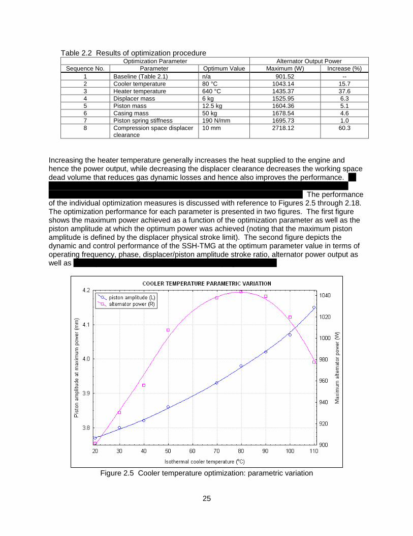
Table 2.2 Results of optimization procedure Optimization Parameter Alternator Output Power

Sequence No. Parameter Optimum Value Maximum (W) Increase (%)

1 Baseline (Table 2.1) n/a 901.52 --

2 Cooler temperature 80 °C 1043.14 15.7

3 Heater temperature 640 °C 1435.37 37.6

4 Displacer mass 6 kg 1525.95 6.3

5 Piston mass 12.5 kg 1604.36 5.1

6 Casing mass 50 kg 1678.54 4.6

7 Piston spring stiffness 190 N/mm 1695.73 1.0

8 Compression space displacer clearance

10 mm 2718.12 60.3

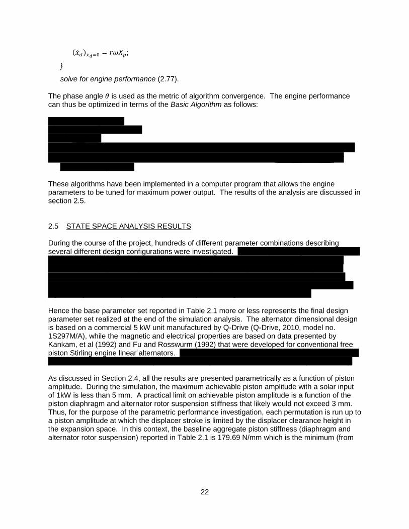
Increasing the heater temperature generally increases the heat supplied to the engine and hence the power output, while decreasing the displacer clearance decreases the working space dead volume that reduces gas dynamic losses and hence also improves the performance. Of interest is that the performance increases with increased cooler temperature (relative to the baseline) which is contradictory, at least from a Carnot efficiency perspective. The performance of the individual optimization measures is discussed with reference to Figures 2.5 through 2.18. The optimization performance for each parameter is presented in two figures. The first figure shows the maximum power achieved as a function of the optimization parameter as well as the piston amplitude at which the optimum power was achieved (noting that the maximum piston amplitude is defined by the displacer physical stroke limit). The second figure depicts the dynamic and control performance of the SSH-TMG at the optimum parameter value in terms of operating frequency, phase, displacer/piston amplitude stroke ratio, alternator power output as well as the displacer motor control stiffness and damping coefficients.

Figure 2.5 Cooler temperature optimization: parametric variation

26

Figure 2.6 Cooler temperature optimization: performance at maximum power

The isothermal cooler temperature performance variation is given in Figures 2.5 and 2.6. Figure 2.5 shows that the piston amplitude increases monotonically with cooler temperature while the alternator power output shows a distinct maximum at 80 °C.

27

Figure 2.7 Heater temperature optimization: parametric variation

Figure 2.6 shows the geometrical increase of alternator power with amplitude while both the amplitude ratio and phase decrease with stroke. The phase between the displacer and piston is positive (that is, displacer leads the piston) and increases with piston stroke. In terms of the control parameters, the damping coefficient increases geometrically and the stiffness linearly with stroke. Note that the stiffness is initially negative (displacer diaphragm stiffness too small, equation (2.61)) becoming positive at a piston stroke of 2 mm (displacer diaphragm stiffness too large). The heater temperature optimization is shown in Figures 2.7 and 2.8. Of interest in Figure 2.7 is the approximately linear increase in alternator power output with temperature corresponding with a highly non-linear relationship between the piston amplitude and the heater temperature between 300 and 400 °C. This arises because at 300 °C, the maximum attainable piston amplitude was 0.5 mm, in other words, the heat input to the engine was too low to sustain robust oscillation. Above 400 °C, the heat input was sufficient to attain a robust oscillation and hence the subsequent amplitude response was monotonic with temperature. From Figure 2.8, again the frequency and phase decline while the phase angle and power increase with piston amplitude. However, in this case, the increase in power is not geometrically dependent on the stroke because of the more significant countervailing effects of decreasing frequency and increasing phase angle (equation (2.77)). Both control parameters show a geometrical increase with amplitude with the damping coefficient reaching a significantly high value in excess of 10,000 kg/s at the maximum piston amplitude.

28

Figure 2.8 Heater temperature optimization: performance at maximum power

29

Figure 2.9 Displacer mass optimization: parametric variation

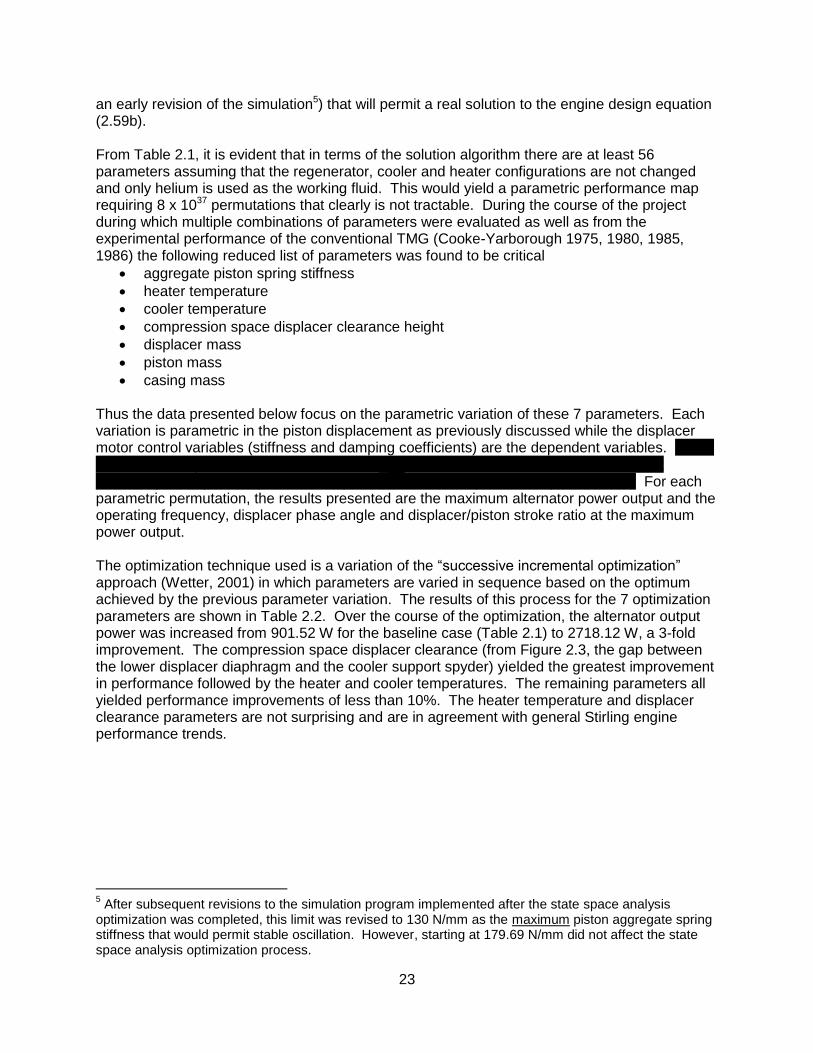
The optimization results for the displacer mass variation are shown on Figures 2.9 and 2.10. Figure 2.9 reveal a distinctly bifurcated engine response in which robust piston oscillation only is possible at displacer masses less than 7 kg. Above 7 kg, the piston amplitude is less than 1 mm and the increase in power with displacer mass is resultant entirely from an increase in frequency (that is low alternator work per engine cycle produced by the small piston stroke being offset by the increasing number of cycles per unit time). Hence the displacer mass necessary for robust oscillation is limited to less than 7 kg and therefore the right-hand half of the optimization is ignored. This yields an optimum displacer mass of 6 kg. At this optimum mass, the engine dynamics conform to the expected patterns as functions of the piston stroke (geometrically increasing power output, decreasing frequency and amplitude ratio and increasing phase angle). The control parameters also conform to the expected pattern with both the stiffness and damping coefficient increasing with amplitude.

30

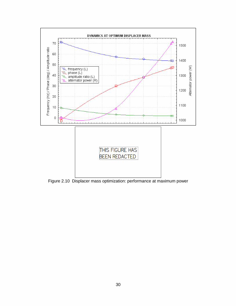
Figure 2.10 Displacer mass optimization: performance at maximum power

31

Figure 2.11 Piston mass optimization: parametric variation

The piston mass optimization phenomenology is revealed in Figures 2.11 and 2.12. Figure 2.11 shows a clear optimum at a piston mass of 12.5 kg both in terms of power and amplitude. Noteworthy in Figure 2.12 is the substantial increase in phase angle from -3.8 to 62 deg. as a function of amplitude while the frequency remains relatively constant at 53 Hz after an initial decline. It may also be observed that at the optimum piston, mass engine operation was only possible at strokes less than 1.07 mm and greater than 4.33 mm. In effect this means, that robust oscillation was only possible at a heat input rate sufficient to produce a piston amplitude of at least 4.33 mm. Lower heat input rates were insufficient.

32

Figure 2.12 Piston mass optimization: performance at maximum power

33

Figure 2.13 Casing mass optimization: parametric variation

The parametric variation of the casing amplitude is depicted in Figures 2.13 and 2.14. Figure 2.14 reveals two distinct operating modes, a low piston amplitude mode below 40kg and a high amplitude mode above 40 kg. In terms of oscillation robustness, the low amplitude mode with a casing mass less than 40 kg is ignored even though it nominally yields the highest power output in terms of the state space analysis6. At the optimum casing mass of 50 kg, Figure 2.14 shows ”typical” SSH-TMG phenomenology as the piston amplitude was increased, specifically increasing phase angle and alternator output power and decreasing frequency and amplitude ratio. Both control parameters increased monotonically with amplitude, with a significant amount of damping required at larger piston amplitudes.

6 Subsequent simulation analysis showed that operation at too low a casing mass eventually caused the

oscillation to cease (over damped condition resulting from insufficient phase difference between the displacer and piston).

34

Figure 2.14 Casing mass optimization: performance at maximum power

35

Figure 2.15 Piston spring stiffness optimization: parametric variation

The aggregate piston spring optimization is shown in Figure 2.15. As a the span of variation is two orders of magnitude, the abscissa is plotted logarithmically. Figure 2.15 also shows two distinct operating regimes, one with a spring stiffness below 500 N/mm and one above it. Above 500 N/mm, the alternator output power remained fairly constant as did the piston amplitude at maximum power. Below 500 N/mm, a varying response was achieved with a clear optimum at 190 N/mm. In practice, this is a crucial design result and shows that the piston suspension stiffness has to be very precisely tuned for optimum performance. This is a challenge in terms of selecting diaphragm materials. Fortunately, there are a range of materials including high temperature plastics that may prove suitable. It may also be necessary to design a special purpose alternator with a freely supported armature to achieve the required level of piston support flexibility. As shown in Figure 2.16, the phenomenology at the optimum piston spring stiffness was fairly typical with control parameters increasing monotonically with increasing piston amplitude.

36

Figure 2.16 Piston spring stiffness optimization: performance at maximum power

37

Figure 2.17 Compression space displacer clearance optimization: parametric variation

Figures 2.17 and 2.18 depict the optimization of the compression space displacer clearance (LCd in figure 2.3). This is a proxy for the “dead” volume of the working space, that is, the volume that remains constant throughout the engine cycle (in this case, it is the clearance between the displacer at bottom dead center and the cooler support spyder that constitutes the dead volume). Generally, Stirling engine theory and experimental results show that the engine performance decreases with increasing dead volume as was the case beyond a clearance of 10 mm. However, the SSH-TMG shows an optimum dead volume because the dead volume is related to the stiffness of the gas spring that also acts on the piston (at a given engine pressurization, decreasing the dead volume increases the gas spring stiffness). Hence, the as the total piston spring stiffness includes both the gas and the mechanical springs, a clear optimum gas spring stiffness is consistent with results of Figure 2.15. The performance at the optimum displacer clearance is revealed in Figure 2.18. Once again, the phenomenology is typical although the damping coefficient shows a clear parabolic trend at higher piston amplitudes.

38

Figure 2.18 Compression space displacer clearance optimization: performance

at maximum power 2.6 CLOSURE

The state space analysis of the SSH-TMG shows that the SSH-TMG does operate successfully and is controllable over a full range of physically reasonable piston amplitudes within the confines of what may be achieved with the fatigue strength of available common materials (metals and plastics). The analysis also reveals that there is a fairly narrow band of parameters in which robust engine oscillation can be achieved, however, this band is well defined. An optimum maximum output power of 2.7kW between isothermal hot and cold temperature limits of 640 and 80 °C respectively (corresponding to a Carnot efficiency of 61%) is possible in terms of the limitations and assumptions of the state space analysis. Further, the control system will support the full range of piston amplitudes so the engine can operate successfully under the actual partial insolation conditions experienced during a diurnal cycle, episodes of cloud cover, etc. 3. SIMULATION ANALYSIS

39

The primary purpose of the simulation analysis was to eliminate the following assumptions and/or limitations included in the state space analysis: a. The isothermal heater was replaced with a full energy balance of the heater including

insolation and the actual heater-to-gas heat transfer using empirical heat transfer coefficients for the fluted heater surface.

b. The isothermal cooler was replaced with a full energy balance of the cooler including the heat removed by the cooling water and the actual heater-to-gas heat transfer using empirical heat transfer coefficients for the fluted cooler surface.

c. Elimination of the assumption of equation (2.6) by independently solving for the transient motion of the casing.

d. Calculating the exact working space dynamic pressure profile and, specifically, the transient pressure profiles in the expansion and compression spaces acting on the piston and displacer. This eliminated the assumption of equation (2.11).

e. Inclusion of the higher order terms in all the linearized equations ((2.23) and (2.33a)). This in turn eliminated the requirement that the piston, displacer and casing motions were sinusoidal (equations (2.42)).

f. The transient alternator current was determined independently so eliminating the assumed dependence on the piston motion expressed by equation (2.43).

g. Improvement of the accuracy of the pressure drop across the displacer tube by calculating the friction factors in the heater, cooler and regenerator on a transient basis as a function of the local Reynolds number. This eliminated the assumption of the friction factors being calculated on a cyclic maximum Reynolds number in equation (2.35).

In addition, the simulation analysis included an entropy transport equation allowing the entropy generation rate in the working space to be determined as part of the engine control system. However, it needs to be noted that the simulation analysis is not a replacement for the state-space analysis in that it does permit the engine optimization process discussed in Section 2.5 to be tractably implemented. Its basic purpose is thus to refine the state-space analysis and provide deeper insight to the operating details of the engine so that a viable prototype eventually may be built. 3.1 SIMULATION EQUATIONS

The dynamic equations are determined from Section 2.3. Substituting (2.36a) into (2.2) and simplifying yields the non-linearized dynamic equation for the displacer:

Substituting (2.41b) into (2.3) and rearranging gives the piston dynamics:

( ) ( )

Lastly for the casing, substituting (2.36a) and (2.41b) into (2.4) and simplifying yields:

( ) ( )

40

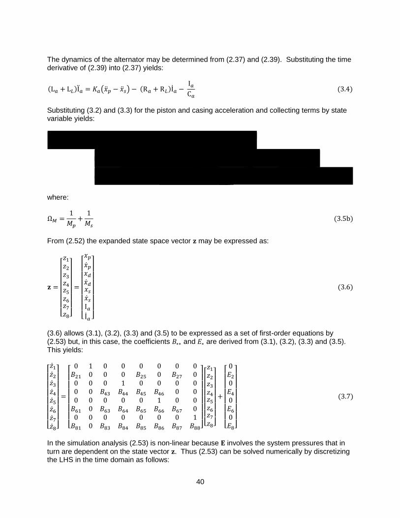
The dynamics of the alternator may be determined from (2.37) and (2.39). Substituting the time derivative of (2.39) into (2.37) yields:

( )

Substituting (3.2) and (3.3) for the piston and casing acceleration and collecting terms by state variable yields:

( )

[ ( )

]

(

)

[

]

where:

From (2.52) the expanded state space vector may be expressed as:

[

]

[

]

(3.6) allows (3.1), (3.2), (3.3) and (3.5) to be expressed as a set of first-order equations by (2.53) but, in this case, the coefficients and are derived from (3.1), (3.2), (3.3) and (3.5). This yields:

[

]

[

]

[

]

[

]

In the simulation analysis (2.53) is non-linear because involves the system pressures that in

turn are dependent on the state vector . Thus (2.53) can be solved numerically by discretizing the LHS in the time domain as follows:

41

which yields:

(

)

From (3.7) this yields:

[

]

[

]

[

]

Owing to its sparseness, (3.9) can be solved efficiently by Gaussian elimination (Gerald, 1973)

yielding an advanced time implicit solution for that is numerically stable. In essence, the purpose of the continuum mechanics numerical simulation of the working

spaces is to provide the pressure terms in the constant . This yields a numerical non-linear solution to (2.53) rather than the approximate analytic linearized solution of (2.55). The details of the continuum mechanics equations used in the simulation analysis are not described here and the reader is referred to Goldberg, 1987a for a detailed and rigorous derivation. The final equation set for the mass, momentum and energy transport in the working spaces as applied to the SSH-TMG may be described in generalized tensor notation for the combined Eulerian-Lagrangian coordinate system needed to describe the engine geometry as follows: Mass transport:

∫ {( ) }

Momentum transport:

42

( )

∫ {( ) }

∫

∫ {( ) }

∫

Energy transport:

( )

∫ {

}

∫ {( ) }

∫ ( )

∫ { ( ) }

The entropy transport equation was derived and experimentally validated in Goldberg, 1992 as a hybrid development of approaches suggested by Slattery (Slattery, 1981) and Truesdell and Toupin (Truesdell and Toupin, 1960) and may be expressed as:

( )

∫

{

}

∫ (

)

∫ { ( ) }

Thus (3.9) through (3.13) provide a complete description of the dynamics and continuum mechanics of SSH-TMG including the heat flows in the solid cooler and heater cores as well as in the solid elements of the regenerator. 3.2 NUMERICAL SOLUTION METHODOLOGY

Equations (3.9) through (3.13) are solved numerically together with an equation of state for the working fluid and experimental heat transfer coefficient and friction factor correlations for the heater, regenerator and cooler.

43

Figure 3.1 Implementation of discretized equations

44

With reference to Figure 3.1, the system is discretized in one-dimension only which is adequate for this level of analysis. Two and three-dimensional effects particularly as they apply to pressure drops and heat transfer are captured by the empirical correlations used. All four continuum mechanics transport equations are applied to the working fluid in the expansion, compression and bounce spaces as well as the heater, cooler and regenerator. The energy transport equation is applied to the heater and cooler cores while the energy and mass transport equations are applied to the coolant in the cooler heat removal chamber. Owing to the movement of the displacer, a combined Eulerian/Lagrangian reference frame is required in order to accurately model the working fluid flow through the displacer tube. As the regenerator is fixed with reference to the SSH-TMG casing (it is sandwiched between the heater and cooler cores) a conventional Eulerian frame of reference is adequate for all the discrete volumes in the regenerator (the displacer tube is separated from the regenerator tube bundle by a clearance gap). All the discrete volumes in the heater and cooler are bounded by combined Eulerian/Lagrangian boundaries. The discrete volumes in the portions of the heater and cooler cores in the expansion and compression spaces respectively utilize Lagrangian boundaries (no fluid flow), while the boundaries within the compression space are Eulerian as the coolant chamber is fixed relative to the casing. The details of the development of the solution algorithm may be found in Goldberg, 1987a. The algorithm is fully implicit and is based on the Semi-Implicit Method for Pressure Linked Equations, Revised (SIMPLER) developed by Patankar (Patankar, 1980) and may be described in prototypical programming language for a single time step as follows: Initialize mass fluxes to current values {

; }

while ( |

| ) {

solve engine dynamics from (3.9); calculate working space geometry as a function of ;

explicitly calculate discrete volume working fluid mass from (3.10) calculate the dependent discrete volume variables (density, viscosity, thermal conductivity,

velocity and pressure gradients, etc.); calculate the friction factors and heat transfer coefficients; solve (3.12) implicitly for the discrete volume temperatures; solve (3.12) for the heater, regenerator and cooler core temperatures and for the coolant

liquid temperature; calculate the coefficients of in (3.11) solve the pressure-linked mass balance implicitly for the discrete volume pressures solve (3.11) implicitly using the pressure field and coefficients for the discrete volume

mass fluxes;

;

;

} time step closure { solve (3.13) implicitly for the discrete volume specific entropy;

45

calculate time step engine performance (heat transfer, indicated and brake work done); } The number of time steps in a cycle is determined by the piston dynamics so that a single cycle is deemed to have been completed when the piston reaches its equilibrium position and has a positive (upwards) velocity, that is, . This allows the engine frequency based on

the piston oscillation to be determined as a dependent function of the engine dynamics. The phase relationships between the engine components are determined from the times during the cycle when they each reach the top dead center of their oscillations. An existing computer program developed by the author was modified to include the engine dynamics and the specific geometry of the SSH-TMG. The salient results of the simulation analysis derived from exercising this program are discussed in the following section. 3.3 SIMULATION ANALYSIS RESULTS

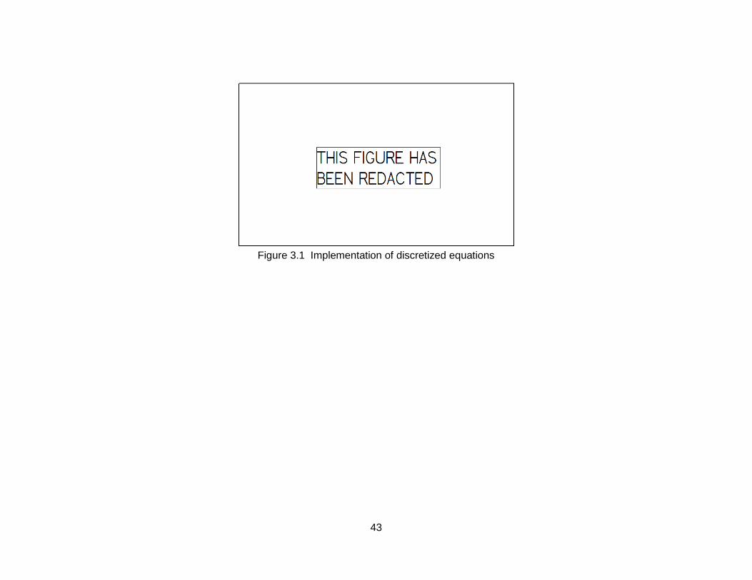
As discussed in Section 2.5, the simulation results are presented for the optimized engine configuration reported in Table 2.1. Table 3.1 shows a compilation of the sensitivity analyses about the optimum verifying that in terms of the seven critical parameters discussed in Section 2.5 (aggregate piston spring stiffness; heater temperature; cooler temperature; compression space displacer clearance height; displacer, piston and casing mass), the engine parameter set is optimized. Clearly in the simulation analysis, the isothermal heater and cooler working fluid temperatures are no longer parameters but are calculated by the simulation. The cooler temperature is replaced as a parameter with the coolant flow rate and supply temperature, while the heater temperature is replaced with the solar power input (insolation). In all the simulations, the coolant supply flow rate and temperature were held constant at 1.5 gpm and 20 °C respectively. The overall size of the engine determines the amount of input power that can be accommodated prior to thermal saturation which occurs when the thermal input is much larger than the mechanical work plus heat rejection. When thermal saturation occurs, the oscillation gradually fades away as the cooler and heater temperatures equilibrate. This is governed strongly by the convective heat transfer in the heater and cooler that, in turn, are dependent on the heat transfer area and flow velocities, both functions of engine size. It was determined that the optimum solar input power handling capacity for the simulation prototype’s size was 800W and so this was the baseline evaluation insolation. The results for the remaining critical parameters (with the exception of the displacer mass) are shown in Table 3.1. The displacer mass was excluded because varying the optimized value of 4.85 kg to any significant extent did not enable a simulated stable oscillation. Each simulation was run until the heater core reached thermal equilibrium, that is, until the cyclic solar thermal heat energy was exactly equal to the cyclic heat transferred to the working fluid. It should be noted, that the number of cycles required for heater equilibrium (reported in Table 3.1) does not represent the number of cycles that would be required by a real prototype, as thermal equilibrium acceleration algorithms are deployed in the simulation to accelerate the process significantly. At heater equilibrium, the coolant chamber had not reached equilibrium because of its very large thermal inertia that requires hours of real-time operation to achieve (days of simulation for each case). Time constraints did not permit this issue to be fully addressed in terms of a more robust acceleration equilibrium for the coolant chamber.

46

Table 3.1 Simulation results for optimized SSH-TMG parameter set with solar input power = 800W

Parameter Parameter

Value

Motor Damping

Coefficient (kg/s)

No. of cycles

Operating Frequency

(Hz)

Disp./ Piston Phase (deg)

Displacer/ Piston

Amplitude Ratio

Piston Amplitude

(mm)

Net Power Output

(W)

Net Brake Efficiency

(%)

Available Cogenerated

Efficiency (%)

Cyclic Average Heater Temp. (°C)

Cyclic Average Cooler Temp. (°C)

Total Cyclic Entropy

Generation Rate (W/K)

Piston aggregate stiffness (N/mm)

130 50 1162 60.28 111.31 2.214 1.742 172.09 21.51 22.84 157.184 145.988 2.291

120 50 1151 60.21 112.26 2.212 1.774 178.765 22.35 23.65 157.414 146.331 2.326

100 50 1145 60.06 114.36 2.203 1.887 203.46 25.43 26.73 158.341 147.695 2.455

60 50 1156 59.76 119.06 2.199 2.015 231.95 28.99 30.3 158.956 148.694 2.558

50 50 1164 59.68 120.24 2.216 2.038 236.9 29.61 30.92 158.953 148.753 2.566

50 25 1354 59.59 119.31 2.178 1.72 200.15 25.02 26.57 154.418 146.629 1.985

40 50 1178 59.6 120.99 2.2 2.055 240.48 30.06 31.39 158.923 148.777 2.564

0 50 1250 59.27 125.08 2.217 2.005 226.95 28.37 29.81 157.791 147.39 2.391

Piston mass (kg)

12.5 25 1357 59.98 114.07 2.156 1.57 181.8 22.72 24.24 152.607 139.936 1.847

12.5 50 1248 60.05 114.4 2.183 1.741 190 23.75 25.19 155.921 144.55 2.161

12.5 60 1151 60.1 113.8 2.191 1.887 207.34 25.92 27.22 158.227 147.601 2.443

Casing mass (kg)

50 50 1356 59.68 111.54 2.226 1.57 128.74 16.09 17.64 152.863 135.75 1.872

Compression Space Displacer Clearance (mm)

10 0 1069 61.47 112.14 2.54 1.273 129.59 16.2 17.57 155.302 143.132 1.655

10 -10 1078 61.45 111.36 2.542 1.193 122.83 15.35 16.68 153.575 140.39 1.555

Table 3.2 Solar power variation for optimized SSH-TMG parameter set (piston stiffness = 40 kg/s; motor damping coefficient = 50 kg/s)

Solar Power Input (W)

No. of cycles

Operating Frequency

(Hz)

Phase (deg)

Displacer/ Piston

Amplitude Ratio

Piston Amplitude

(mm)

Net Power Output

(W)

Carnot Efficiency

(%)

Net Brake Efficiency

(%)

Available Cogenerated

Efficiency (%)

Total Cyclic

Entropy Generation

Rate (W/K

State Space Analysis

Alternator Power Output

(W)

Error (%)

1000 764 59.45 123.72 2.216 2.075 243.19 42.5 24.32 24.76 3.054 226.98 6.7

900 958 59.54 121.66 2.205 2.07 243.4 42 27.04 27.83 2.821 238.99 1.8

800 1178 59.6 120.99 2.2 2.055 240.48 41.5 30.06 31.39 2.564 249.26 3.7

47

Figure 3.2 Aggregate piston spring stiffness variation phemonenology

The acceleration algorithm that was deployed, in any case, increased the rate of coolant chamber equilibration by several orders of magnitude, but was insufficient for the achievement of full thermal equilibrium. Thus the amount of heat rejected to the coolant at heater core thermal equilibrium is too low resulting in an underestimate of the cogenerated efficiency. The salient performance issue revealed in Table 3.1, are the low heater and high cooler gas temperatures relative to the optima found in Section 2.5 from the state space analysis. The

48

optimum isothermal gas temperature of 640 °C is 482 °C higher than the 158.2 °C cyclic average of the simulation prototype, while the optimum isothermal cooler gas temperature of 80 °C is 68 °C greater than 147.7 °C cyclic average of the simulation prototype. This arises because the insolation required to achieve such a high heater temperature is a multiple of the 800 W power capacity of the prototype and is far too large for it size. This scaling issue cannot be resolved by an isothermal analysis as alluded to previously. The higher cooler temperature, on the other hand, is an indication that the cooling capacity of the simulation prototype is inadequate and is likely the largest issue with the current design. The specific issue is the thermal coupling of the coolant to the working fluid that is far too small in the current design. The coupling is limited by the conductivity of the solid cooler core, and more significantly, the low heat transfer area between the cooler core and the coolant in the coolant chamber (see Figures 3.6 and 3.7). Thus improving the cooler design is be a key priority for future work. The other key thermal issue is the small temperature drop across the regenerator averaging just 10.6 °C in the simulation prototype compared with 560 °C in the isothermal prototype. This is a function of the regenerator thermal effectiveness. As discussed previously, it transpired that the pressure drop of the originally proposed stacked wire gauze regenerator that has a relatively high effectiveness was way too large for the simulation prototype and choked off oscillation. Replacing this with a tube bundle regenerator decreased the pressure drop to a reasonable level, but at the expense of regenerator effectiveness as shown by the results. This is a classic dilemma in Stirling engine design in which the overall thermal performance is strongly dependent on the regenerator effectiveness. However, as a resonant system, the SSH-TMG is equally sensitive to the regenerator pressure drop, hence balancing these competing requirements is challenging. Thus improving the regenerator to achieve a greater thermal effectiveness without a significant increase in pressure drop also would be a priority for future work. In additional to the basic dynamics variables (frequency, displacer/piston phase and amplitude ratio), the net power output, net brake efficiency, available cogenerated efficiency and the total cyclic entropy generation rate also are reported in Table 3.1. The net power output is the sum of the power output of the alternator plus/minus the power required to operate the displacer tuning linear alternator/motor7. Thus the brake efficiency represents the electrical power at the engine output terminals divided by the solar input power. The available cogenerated efficiency is the heat rejected by the coolant plus the net electrical power output divided by the solar input power. As discussed above, these results are an underestimate of the expected performance at full engine equilibrium. The total cyclic entropy generation rate is a measure of the irreversibility in the working spaces and quantifies the impacts of pressure and temperature gradients as well as turbulence on the engine performance. The optimum displacer tuner control parameters for the simulation prototype were a damping coefficient of 50 kg/s with both the stiffness and offset coefficients set to 0. Table 3.1 shows some variations of the damping coefficient to indicate their effect in particular cases. The aggregate piston spring stiffness proved to be the most sensitive parameter. The initial spring stiffness of 179.69 N/mm was based on a fairly early revision of the simulation program.

7 If the displacer tuner acts as a motor, the net power output of the SSH-TMG is the alternator power

output minus the tuner power input. If the tuner acts as an alternator, the net power output is the alternator output plus the tuner power output.

49

Figure 3.3 Displacement temporal profiles at maximum efficiency

Subsequent modifications, bug fixes and corrections to the simulation program performed after the state space optimization exercise had been completed resulted in this value being too large. Stable oscillation with the final revision of the program would only commence at a much lower value of maximum spring stiffness of about 130 N/mm. The variation of the spring stiffness for the simulation prototype is shown in Figure 3.2. The maximum net power output of 240.48 W was achieved at a stiffness of 40 N/mm that also corresponded to the maximum brake efficiency of 30% and a cogenerated efficiency of 31%. Based on the degree of coolant chamber convergence, the ultimate cogenerated efficiency at full convergence may be expected to be greater than 60%. It is unlikely that a stiffness of 40 N/mm can be achieved by a metal piston diaphragm, and thus a polymer diaphragm would be more appropriate. A suitable candidate polymer material is polyetheretherketone (PEEK) that has a maximum service temperature range of 230 to 315 °C (MatWeb, 2011), that is at least 80 °C greater than the average cyclic cooler working fluid temperature (the compression space temperature at the diaphragm face is lower still). The engine dynamics (lower panel in Figure 3.2) showed a fairly uniform operating frequency of 60 Hz (standard US electrical grid frequency).

50

Figure 3.4 Velocity temporal profiles at maximum efficiency

The displacer leads the piston by between 111 and 125 deg. with the phase angle decreasing with spring stiffness. The piston amplitude profile tracked that of the net power output with a maximum value of 2.06 mm. This level of amplitude is physically reasonable for the optimum level of spring stiffness and is within the fatigue limits of suitable diaphragm materials such as PEEK8. The amplitude ratio remained very uniform with a value of 2.2. The parametric variations in Table 3.1 were applied separately, not sequentially as in Section 2.5. This is intended as a sensitivity analysis, not to refine the optimization already realized in Table 2.1. Any significant variation of the piston mass, similar to the displacer mass variation, failed to produce a stable oscillation.

8 Wolf Kunststoff ZEDEX® ZX-324 A3A PEEK has a fatigue strength of 60MPa (MatWeb, 2011) while the

imposed pressure load (maximum bounce space / compression space pressure differential) at maximum power is about 0.12 MPa (see Figure 3.5). Maximum continuous service temperature for this material is 250 °C.

51

Figure 3.5 Pressure temporal profiles at maximum efficiency

Thus keeping the piston mass at the optimum value and varying the displacer tuning motor damping coefficient, did produce an increase in net output power as the damping coefficient was increased. However, the maximum power of 207 W was significantly less than the overall maximum of 240 W. Increasing the casing mass to 50 kg from the optimum value of 46 kg (Table 2.1) significantly lowered the net output power from 237 W to 139 W, confirming the optimality of the casing mass. A smaller casing mass failed to produce a stable oscillation. Similarly, decreasing the compression space displacer clearance from the optimum value of 23 mm (Table 2.1) to the state space analysis optimum of 10 mm decreased the net power output from 237 W to 130 W that could only be achieved when the displacer control motor damping coefficient was reduced to 0 kg/s. Decreasing the damping coefficient to -10 kg/s, further decreased the power to 123 W. The cyclic SSH-TMG dynamics at the maximum simulated brake efficiency of 30% are shown in Figures 3.3 to 3.5. Figure 3.3 confirms that all the piston, displacer and casing oscillations were perfectly sinusoidal confirming the validity of the argument yielding equations (2.42). Figure 3.4 likewise shows that the piston, displacer and casing velocities were also perfectly sinusoidal as

52

must necessarily be the case. However, Figure 3.5 demonstrates that the expansion and compression space pressure profiles were not sinusoidal, most notably the expansion space profile around the cyclic maximum pressure. This is evidence of the non-linearities resultant from the dissipation in the heater, cooler and regenerator. Finally, the all-important impact of varying the insolation is shown in Table 3.2. As the solar power input is increased beyond the saturation limit of 800 W, the net power output increases slightly (about 2.5 W at 1000 W) but the brake efficiency drops significantly by about 6 % at 1000 W. This appears to be a key characteristic of the SSH-TMG, namely a power output that is fairly stable with varying input power, but an efficiency that is very sensitive to input power. This is also an aspect of the engine that needs to be investigated more thoroughly in future work. Table 3.2 also compares the results produced by the state space and simulation analyses in terms of the net electrical power output. When the state space analysis is applied using the simulated average cyclic heater and cooler temperatures and the simulated piston displacement, the state space analyis and simulation agree within 7%, which, given the isothermal assumption inherent in the state space analysis, is perhaps better than expected. However, the fact that the prototype engine can achieve an efficiency of 30% at an input power of just 800 W is very promising, since the data show that achieving a higher power handling capacity can be readily realized by increasing the size of the engine that likely would not have a major detrimental effect on the efficiency. Bearing in mind that the project target, as expressed in the project proposal, was an output power level of 1-2 kW with an electrical efficiency greater than 20% and a cogenerated efficiency greater than 60%, Table 3.2 shows an electrical efficiency (equivalent to the technically more accurate brake efficiency) of 30% at 240W. Thus scaling the engine up to 1 kW, a factor of about 4, would require doubling the size of the engine in terms of the piston diameter, as the force applied to the alternator (and hence the rate of work transfer) is proportional to the area. Thus, from Figure 3.7, a 1 kW engine can be expected to have a piston diameter of 268 mm (about 11 in.) which is physically reasonable. Unfortunately, there was insufficient time in the project to develop and optimize a larger simulation prototype. However, the level of performance achieved is very competitive with a “state-of-the-art” commercial photovoltaic panel, such as the recently announced SANYO HIT-N225A019 with a rated output power of 225 W at a module efficiency of 17.8% (Sanyo, 2011). 4. SIMULATION PROTOTYPE DESIGN The design of the simulation prototype SSH-TMG is shown in Figures 3.6 and 3.7. Figure 3.6 shows the overall engine dimensions based on a commercially available linear alternator as a reference.

9 Current cost range from the WWW is $599 to $891 for a single panel

(http://www.google.com/products/catalog?q=SANYO+HIT-N225A01&rls=com.microsoft:en-us:IE-Address&oe=&um=1&ie=UTF-8&tbm=shop&cid=1111976078355401415&os=sellers&sa=X&ei=jnZNTrK_J8aHsgKc1rjyBg&ved=0CCUQ_QgwAQ#).

53

Figure 3.6 SSH-TMG overall final design

54

Figure 3.7 SSH-TMG overall final design working space detail

55

As the overall size of the engine of 534 mm (21 in.) is governed by the diameter of the linear alternator, with the example shown having a diameter of about 366 mm (14.4 in.), there is plenty of scope to double and even treble the maximum diameter of the SSH-TMG module itself (Figure 3.7) to achieve a maximum electrical power output of 1800 W or more. The overall engine dimensions reflect those of Table 2.1. The heater, regenerator and cooler reflect the outcome of the engine optimization process as discussed in Section 3.3. The design of the heater as a solid core with a fluted surface to promote convective heat transfer to the working fluid was shown to be acceptable. A similar design for the cooler in which the solid cooler core fin projects into the coolant stream was demonstrated to yield insufficient heat rejection. An alternate cooler design, perhaps consisting of an annular plate heat exchanger, will likely prove far more effective and easier to implement physically on a larger scale engine. The bundled tube regenerator was effective in yielding an adequately low pressure drop, however, at the expense of too low a thermal effectiveness. Improving the effectiveness without too large a pressure drop penalty is a design challenge for the future that also should be easier to realize at a bigger engine scale. The balance of the design closely follows that of the conceptual design discussed in Section 2.1. 5. CONCLUSION The project has successfully demonstrated that the SSH-TMG does operate and exceeds its performance target in terms of net electrical efficiency. The maximum electrical power output of 240 W realized by the optimized prototype engine simulated was achieved at an efficiency of 30% compared with a target of 1-2 kW electrical output at greater than 20% efficiency. However, the prototype design can be readily scaled up by a factor of 2 or 3 to realize the target output power range. The results achieved with the simulation prototype compare favorably with that of a recently announced high performance commercial photovoltaic panel producing 225 W at a module efficiency of 17.8%. The full cogenerated performance of the engine was not fully demonstrated owing to an insufficiency of time to address the algorithmic issues involved. The state space and simulation analyses used to develop the SSH-TMG were shown to agree within 7% indicating that the state space analysis is an effective design and optimization tool provided that the isothermal heater and cooler working fluid temperatures are consistent with those that can be achieved for a given level of insolation and achievable heat rejection using a practical heat removal system. The results also demonstrate that the key components of the engine requiring further improvement are the regenerator and the cooler. The regenerator needs to be optimized to achieve a higher thermal effectiveness without a substantial increase in pressure drop. The cooler design proved to be inadequate and needs to be redesigned to significantly increase the thermal coupling between the working fluid and the coolant. The design and optimization exercise did not reveal the need for any exotic materials or unusual fabrication processes, so there is no reason to suppose that a scaled-up engine with an output power of about 1800 W would not be cost competitive with the reference photovoltaic panel (225 W Sanyo HIT) that would have a minimum equivalent cost of about $4,800.

56

6. PROGNOSIS As the SSH-TMG is University intellectual property (IP), it would be difficult to proceed with externally funded further development work unless the IP is provided with suitable patent protection. The research completed in this project provides ample justification for seeking such patent protection and that is suggested as a reasonable next step. In terms of further development of the engine, it would be necessary to continue with further analysis prior to undertaking the expensive exercise of developing and testing a physical prototype. This further analysis should focus on the following:

Scale the simulation prototype up in terms of diameter by a factor of 3 with the objective of achieving an electrical output power of 1800 W.

Optimize the regenerator to increase its effectiveness without increasing the flow pressure drop significantly.

Redesign the cooler to significantly increase its ability to remove heat from the engine.

Refine the cooler convergence acceleration algorithm to allow full thermal convergence of the cooler concomitant with full thermal convergence of the heater.

REFERENCES 3d Lens Corporation, 2010. WWW: www.3dlens.com Benvenuto, G., 1994. Electrodynamic analysis of the HARWELL Thermo-mechanical Generator: Comparison of theoretical and experimental results, Proc. 29th Intersoc. Energy Conversion Eng. Conf., vol. 4, pp. 1866-1872. Benvenuto, G. and F. de Monte, 1995a. Analysis of Free-Piston Stirling/Linear Alternator Systems Part I: Theory, J. Propulsion and Power, vol. 11, no. 5, pp. 1036-1046. Benvenuto, G. and F. de Monte, 1995b. Analysis of Free-Piston Stirling/Linear Alternator Systems Part 2: Results, J. Propulsion and Power, vol. 11, no. 5, pp. 1047-1055. Bird R.B., W.E. Stewart and E.N. Lightfoot, 1960. Transport Phenomena, John Wiley & Sons, New York. Cooke-Yarborough, E.H., 1975. Efficient Thermo-Mechanical Generation of Electricity from the Heat of Isotopes, Proc. 10th Intersoc. Energy Conversion Eng. Conf, no. 759150, pp1003-1011. Cooke-Yarborough, E.H., 1980. Small Stirling-cycle Power Sources in Marine Applications, OCEANS 1984, vol. 12, pp. 457-462. Cooke-Yarborough, E.H., 1985. Articulated Diaphragms for Thermo-Mechanical Generators, Proc. 20th Intersoc. Energy Conversion Eng. Conf. ,paper no. 859426, vol. 3, pp. 338-343. Cooke-Yarborough, E.H., 1986. Use of an Analogue Modelling Program to Study the Dynamics of a Thermo-Mechanical Generator, Assoc Termotecnica Italiana, vol. 2, pp. 539-556. Creswick, F.A. Thermal Design of Stirling Cycle Machines, Trans. SAE, paper no. 650079.

57

Fu, Z.X. and M.Rosswurm, 1992. Tradeoff Between Magnet Volume and Tuning Capacitor in a Free Piston Stirling Engine Power Generation System, Proc. 27th IECC, vol. 5, pp. 5.295-5.302. Finkelstein, T., 1960. Generalized Thermodynamic Analysis of Stirling Engines, SAE, paper no, 118B. Garimella, S. and R.N. Christenson, 1995a. Heat Transfer and Pressure Drop Characteristics of Spirally Fluted Annuli: Part II – Hydrodynamics, J. Heat Transfer, vol. 117, pp. 54-60. Garimella, S. and R.N. Christenson, 1995b. Heat Transfer and Pressure Drop Characteristics of Spirally Fluted Annuli: Part II – Heat Transfer, J. Heat Transfer, vol. 117, pp. 61-68. Gerald, C.F., 1973. Applied Numerical Analysis, Addison-Wesley, Reading, MA. Goldberg, L.F. 1992. An Investigation of the Information Propagation and Entropy Transport Aspects of Stirling Machine Numerical Simulation, NASA Contractor Report 189143, Lewis Reseach Center. Goldberg, L.F. 2010a. Net-zero energy systems quantitative scoping analysis (in Performance-based research on housing and infrastructure development at UMore Park), Final Report, Energy Systems Design Program, College of Design, University of Minnesota. Goldberg, L.F. 2010b. Hybrid Energy System Revision III (HES III), Office of Technology Commercialization, Docket no. ROI201000111, University of Minnesota. Goldberg, L.F., 1987a. A State Space and Continuum Mechanics Analysis of Stirling Cycle Machines, Ph.D Thesis, University of the Witwatersrand, South Africa. Goldberg, L.F., 1987b. Simulated Systems Impact of Two-Dimensional Oscillating Flows in a Stirling Machine Heat Exchanger, ASME, Fluids Engineering Div., vol. 62, pp. 63-68. Goldberg, L.F. and K.P. Lee, 1985. 'The Design and Simulation Investigation of a Linear Alternator Dynamometer Coupled to a Free Piston Stirling Engine, Proc. 20th Intersoc. Energy Conversion Eng. Conf., paper no. 859073, vol. 3, pp. 218-223. Goldberg, L.F., 1983 The Application of Non-Linear, State Space Stability Analyses to Free Piston Stirling Engine Design, Proc. 18th Intersoc. Energy Conversion Eng. Conf., paper no. 839123, vol. 2, pp. 761-765. Goldberg, L.F., 1980 A State Space Analysis of a Symmeterical Compounded Free Piston Stirling Engine, Proc. 15th Intersoc. Energy Conversion Eng. Conf., pp. 2251-2257. Goldberg, L.F. and C.J. Rallis, 1979 A Prototype Liquid-Piston Free-Displacer Stirling Engine, Proc. 14th Intersoc. Energy Conversion Eng. Conf., pp. 1103-1108. Kankam, M.D., J.S.Rauch and W. Santiago, 1992. Dynamic Analysis of Free-Piston Stirling Engine/Linear Alternator-Load System – Experimentally Validated, Proc. 27th IECC, vol. 5, pp. 5.315-5.323. Kays, W.M. and , A.L. London, 1964. Compact Heat Exchangers, McGraw Hill, New York.

58

MatWeb, 2011. URL: www.matweb.com. Nickalls, R.W.D., 1993. Cardan’s solution revealed, The Mathematical Gazette, vol. 77, no. 480, pp. 354–359. Patankar, S.V., 1980. Numerical Heat Transfer and Fluid Flow, Hemisphere, Washington D.C. Q-Drive, 2010. www.qdrive.com. Redlich, R.N. and D.M. Berchowitz, 1985. Linear Dynamics of Free-Piston Stirling Engines, Proc. I. Mech. Eng., vol. 199, A3, pp. 203-213. Sanyo, 2011. URL: http://us.sanyo.com/News/SANYO-HIT-POWER-Solar-Panels-Produce-More-Power-with-New-225A-for-US-Market Slattery, J.C., 1981. Momentum, Energy, and Mass Transfer in Continua, Robert E. Krieger, New York. Sundrum Solar, 2010. URL: www.sundrumsolar.com Truesdell, C. and R.A. Toupin, 1960. In “Handbuch der Physik”, Flugge, S. (editor), vol. 3/1, Springer-Verlag, Berlin. Wetter, M. 2001. GenOpt®, Generic Optimization Program. Seventh International IBPSA Conference, Rio de Janeiro, Brazil.