HARNESSING TUNNELS FOR DIRTY-SLATE NETWORK SOLUTIONS

Hitesh Ballani, Ph.D.

Cornell University 2009

The tremendous success of the Internet has been both a boon and bane for net-

working research. On one hand, Internet growth has led to a plethora of prob-

lems and has prompted work towards next-generation network architectures.

While very important, the success of the Internet has also meant that such clean-

slate proposals are difficult to deploy. Thus, it is imperative that we find prac-

tically deployable dirty-slate solutions. In this thesis, we explore the possibility

of tackling network problems in the existing framework through the use of tun-

nels. Tunneling involves encapsulating protocols in each other and we argue

that this can serve as an enabler to the use of existing protocols in novel ways.

We have found that, in many cases, such an approach can be used to address

the root cause of a problem afflicting the network without necessitating protocol

changes. Further, the increasing adoption of tunnels in mainstream networks

augurs well for the deployability of such tunnels-based solutions.

In this thesis, we focus on two important network problems and present

tunnel-driven, dirty-slate solutions to address them. The first problem is rout-

ing scalability and includes the growing size of the Internet routing table. We

note that routing table size is problematic since every router is required to main-

tain the entire table. Consequently, we propose ViAggre (Virtual Aggregation), a

scalability technique that uses tunnels to ensure that individual routers only

maintain a fraction of the global routing table. ViAggre is a “configuration-

only” approach to shrinking the routing table on routers – it does not require

any changes to router software and routing protocols and can be deployed in-

dependently and autonomously by any ISP. We present the design, evaluation,

implementation and deployment of ViAggre to show that it can offer substantial

reduction in routing table size with negligible overhead.

The second part of the thesis delves into IP Anycast. The route-to-closest-

server abstraction offered by IP Anycast makes it an attractive primitive for

service discovery. Further, the growth of P2P, overlay and multimedia appli-

cations presents new uses for IP Anycast. Unfortunately, IP Anycast suffers

from serious limitations – it is difficult to deploy, scales poorly and lacks im-

portant features like load balancing. As a result, its use has been limited to a

few critical infrastructure services like DNS root servers. Further, despite such

deployments, the performance of IP Anycast and its interaction with IP routing

practices is not well understood.

While these are valid concerns, we also believe that IP Anycast has com-

pelling advantages. Motivated by these, we first conduct a detailed study of IP

Anycast that equips us with the knowledge of how to maximize its potential.

Building upon this, we present PIAS (Proxy IP Anycast Service), an anycast ar-

chitecture that uses tunnels and proxies to decouple the anycast service from

Internet routing. This allows PIAS to overcome IP Anycast’s limitations while

largely maintaining its strengths. We present simulations, measurement results,

implementation and wide-area deployment details and describe how PIAS sup-

ports two important P2P and overlay applications.

BIOGRAPHICAL SKETCH

The author of this thesis hails from New Delhi, India where he spent his forma-

tive years trying to get ready the face the real world. Almost as a rite of passage,

he went to an engineering school in Roorkee, a sleepy little town in Northern In-

dia. Feeling that he was not equipped to brave the rigors of the big bad world,

he chose to extend his cloistered life by enrolling in Cornell’s Ph.D. program.

At Cornell, he spent six wonderful years relishing the myriad joys of Ithaca, a

sleepy little town in Upstate New York. He also dabbled in some research on

the side. While the completion of this document suggests that the author has

worn out his welcome at Cornell, he still does not feel up to the challenge posed

by what is “out there” and is in the midst of planning his next (possibly sleepy

little town) venture.

iii

This document is dedicated to Ma, Papa, Neha and Erin.

iv

ACKNOWLEDGEMENTS

Paul Francis has been the perfect advisor for me. Despite the popular perception

about his laissez-faire attitude towards student development, my graduate life

suggests that he always had a plan for me. He nurtured me patiently while I

learned the ropes of research. Then, he encouraged me to think independently,

but was available if I got stuck (which I did). And when I was finally able to do

research on my own, he gave me the space to do so. All this while, he has been

very patient regarding all my follies.

While Paul has had a profound influence on the way I perceive networking

research and think about what lies ahead, his biggest gift to me is a sense of

equanimity about research and life in general. As a researcher, it is important

to be able to maintain a healthy dose of skepticism, but not to cross over to

cynicism. I believe that Paul has struck a good balance in this regard and I can

only hope to do the same. The past six years have been very fulfilling and truly

amazing, and I owe Paul a lot for that.

AndrewC.Myers andMartin T.Wells were kind enough to agree to bemem-

bers of my thesis committee. I have often relied on Andrew for advice on mat-

ters outside Paul’s expertise. He painstakingly read this entire thesis and his

comments have contributed significantly to the quality of my writing. I have

been fortunate to have had two excellent mentors, Sylvia Ratnasamy and Pablo

Rodriguez, over the course of my internships. Sylvia’s unbridled enthusiasm

has influenced my outlook on research and I am grateful for that.

My graduate work, some of which is discussed in this thesis, includes contri-

butions from many people. Jia Wang and Nikolaos Laoutaris were very helpful

collaborators. Tuan Cao did most of the heavy lifting on the ViAggre imple-

mentation; he was a pleasure to work with. I am proud of the fact that I de-

v

ployed an IP Anycast testbed, and have been maintaining it for the past few

years. This was made possible through the gracious help and support of the

following: Eric Cronise, Dan Eckstrom and Larry Parmelee at Cornell Univer-

sity, James Gurganus, Phil Buonadonna, Timothy Roscoe and Sylvia Ratnasamy

at Intel-Research, Kaoru Yoshida, Akira Kato and Yuji Sekiya at WIDE, and JJ

Jamison and Tony Talerico at Cisco.

A lot of credit goes to people who have borne my antics and humored me

during my stay at Cornell. This includes the Systems Lab crowd: Mahesh Bal-

akrishnan, Tuan Cao, Oliver Kennedy, Jed Liu, Tudor Marian, Rohan Murty,

Amar Phanishayee, Alan Shieh, Dan Williams and Xinyang Zhang. Outside the

lab, Lucian Leahu, Jonathan Petrie, Radu Popovici, Vidhyashankar Venkatara-

man and Jonathan Winter helped me keep my mind off work. A special word

of thanks to Jed, Mahesh and Vidhya for all the spots at Teagle. Finally, my life

at Cornell was made much easier due to the physical proximity to Saikat Guha.

His desk was next to mine, and I cannot recall the number of times he saved my

skin. Kudos to him for being an amazingly smart and helpful colleague.

Graduate school would not have been possible without the support of my

parents. They have worked very hard and sacrificed too much to make sure that

I was able to pursue all my dalliances. I can never thank them enough. Neha

and Nana kept me on my toes with their persistent yet well-meaning queries

about the progress of my thesis. Hazel-cat provided much needed entertain-

ment during the writing of this thesis. Her walks across my keyboard con-

tributed immensely to the thesis; though I hope most of her contributions have

been edited out. And last but not the least, Erin, with her love, affection, amaz-

ing culinary skills and enlightened taste in music, has added oodles of joy to my

existence. Thank you all.

vi

TABLE OF CONTENTS

Biographical Sketch . . . . . . . . . . . . . . . . . . . . . . . . . . . . . . iiiDedication . . . . . . . . . . . . . . . . . . . . . . . . . . . . . . . . . . . ivAcknowledgements . . . . . . . . . . . . . . . . . . . . . . . . . . . . . . vTable of Contents . . . . . . . . . . . . . . . . . . . . . . . . . . . . . . . viiList of Figures . . . . . . . . . . . . . . . . . . . . . . . . . . . . . . . . . ixList of Tables . . . . . . . . . . . . . . . . . . . . . . . . . . . . . . . . . . xii

1 Introduction 11.1 Routing Scalability . . . . . . . . . . . . . . . . . . . . . . . . . . . 41.2 IP Anycast Scalability . . . . . . . . . . . . . . . . . . . . . . . . . . 61.3 Outline . . . . . . . . . . . . . . . . . . . . . . . . . . . . . . . . . . 11

2 All About Tunnels 13

3 Virtual Aggregation (ViAggre) 173.1 Background and Contributions . . . . . . . . . . . . . . . . . . . . 173.2 ViAggre design . . . . . . . . . . . . . . . . . . . . . . . . . . . . . 21

3.2.1 Design Goals . . . . . . . . . . . . . . . . . . . . . . . . . . 223.2.2 Design-I: FIB Suppression . . . . . . . . . . . . . . . . . . . 243.2.3 Design-II: Route Reflectors . . . . . . . . . . . . . . . . . . 283.2.4 Design Comparison . . . . . . . . . . . . . . . . . . . . . . 293.2.5 Network Robustness . . . . . . . . . . . . . . . . . . . . . . 303.2.6 Routing popular prefixes natively . . . . . . . . . . . . . . 30

3.3 Allocating aggregation points . . . . . . . . . . . . . . . . . . . . . 313.3.1 Problem Formulation . . . . . . . . . . . . . . . . . . . . . 323.3.2 A Greedy Solution . . . . . . . . . . . . . . . . . . . . . . . 35

3.4 Evaluation . . . . . . . . . . . . . . . . . . . . . . . . . . . . . . . . 373.4.1 Metrics of Interest . . . . . . . . . . . . . . . . . . . . . . . 383.4.2 Tier-1 ISP Study . . . . . . . . . . . . . . . . . . . . . . . . . 393.4.3 Rocketfuel Study . . . . . . . . . . . . . . . . . . . . . . . . 493.4.4 Discussion . . . . . . . . . . . . . . . . . . . . . . . . . . . . 50

3.5 Deployment . . . . . . . . . . . . . . . . . . . . . . . . . . . . . . . 513.5.1 Configuration Overhead . . . . . . . . . . . . . . . . . . . . 543.5.2 Control Plane Overhead . . . . . . . . . . . . . . . . . . . . 553.5.3 Failover . . . . . . . . . . . . . . . . . . . . . . . . . . . . . 58

3.6 Discussion . . . . . . . . . . . . . . . . . . . . . . . . . . . . . . . . 593.7 Related Work . . . . . . . . . . . . . . . . . . . . . . . . . . . . . . 623.8 Summary . . . . . . . . . . . . . . . . . . . . . . . . . . . . . . . . . 64

vii

4 IP Anycast Measurement Study 664.1 Overview . . . . . . . . . . . . . . . . . . . . . . . . . . . . . . . . . 664.2 Related Measurement Studies . . . . . . . . . . . . . . . . . . . . . 704.3 Deployments Measured . . . . . . . . . . . . . . . . . . . . . . . . 714.4 Methodology . . . . . . . . . . . . . . . . . . . . . . . . . . . . . . 764.5 Proximity . . . . . . . . . . . . . . . . . . . . . . . . . . . . . . . . . 794.6 Failover time . . . . . . . . . . . . . . . . . . . . . . . . . . . . . . . 884.7 Affinity . . . . . . . . . . . . . . . . . . . . . . . . . . . . . . . . . . 944.8 Client Load Distribution . . . . . . . . . . . . . . . . . . . . . . . . 994.9 Discussion . . . . . . . . . . . . . . . . . . . . . . . . . . . . . . . . 1044.10 Summary . . . . . . . . . . . . . . . . . . . . . . . . . . . . . . . . . 107

5 Proxy IP Anycast Service 1095.1 Overview . . . . . . . . . . . . . . . . . . . . . . . . . . . . . . . . . 1095.2 Design Goals . . . . . . . . . . . . . . . . . . . . . . . . . . . . . . . 1115.3 Design Description . . . . . . . . . . . . . . . . . . . . . . . . . . . 113

5.3.1 The Join Anycast Proxy (JAP) . . . . . . . . . . . . . . . . . 1165.3.2 Scale by the number of groups . . . . . . . . . . . . . . . . 1185.3.3 Scale by group size and dynamics . . . . . . . . . . . . . . 1215.3.4 Scale by number of proxies . . . . . . . . . . . . . . . . . . 1225.3.5 Proximity . . . . . . . . . . . . . . . . . . . . . . . . . . . . 1255.3.6 Robustness and fast failover . . . . . . . . . . . . . . . . . . 1265.3.7 Target selection criteria . . . . . . . . . . . . . . . . . . . . . 128

5.4 Evaluation . . . . . . . . . . . . . . . . . . . . . . . . . . . . . . . . 1325.4.1 Scalability by group size and dynamics . . . . . . . . . . . 1325.4.2 Stretch . . . . . . . . . . . . . . . . . . . . . . . . . . . . . . 1365.4.3 Implementation . . . . . . . . . . . . . . . . . . . . . . . . . 138

5.5 Related work . . . . . . . . . . . . . . . . . . . . . . . . . . . . . . . 1385.6 Anycast applications . . . . . . . . . . . . . . . . . . . . . . . . . . 141

5.6.1 Peer Discovery . . . . . . . . . . . . . . . . . . . . . . . . . 1415.6.2 Reaching an Overlay network . . . . . . . . . . . . . . . . . 142

5.7 Discussion . . . . . . . . . . . . . . . . . . . . . . . . . . . . . . . . 1435.8 Summary . . . . . . . . . . . . . . . . . . . . . . . . . . . . . . . . . 145

6 Concluding Remarks 146

Bibliography 148

viii

LIST OF FIGURES

3.1 Router Innards: A router exchanging routing information withtwo neighboring routers. . . . . . . . . . . . . . . . . . . . . . . . 18

3.2 A ViAggre ISP with four virtual prefixes (0/2, 64/2, 128/2,192/2). The virtual prefixes are color-coded with each routerserving as an aggregation point for the corresponding color. Thered routers are aggregation points for the 0/2 virtual prefix andadvertise it into the ISP’s internal routing. . . . . . . . . . . . . . 25

3.3 Path of packets destined to prefix 4.0.0.0/24 (or, 4/24) betweenexternal routers A and E through an ISP with ViAggre. Router Cis an aggregation point for virtual prefix 4.0.0.0/7 (or, 4/7). . . . 27

3.4 FIB composition for the router with the largest FIB, C=4ms andno popular prefixes. . . . . . . . . . . . . . . . . . . . . . . . . . . 41

3.5 Variation of FIB Size and Stretch with Worst Stretch constraintand no popular prefixes. . . . . . . . . . . . . . . . . . . . . . . . . 43

3.6 Variation of the percentage of traffic stretched/impacted andload increase across routers with Worst Stretch Constraint (Uni-form Allocation) and no popular prefixes. . . . . . . . . . . . . . 45

3.7 Popular prefixes carry a large fraction of the ISP’s traffic. . . . . . 473.8 Variation of Traffic Impacted and Load Increase (0-25-50-75-100

percentile) with percentage of popular prefixes, C=4ms. . . . . . 483.9 FIB size for various ISPs using ViAggre. . . . . . . . . . . . . . . . 493.10 WAIL topology used for our deployment. All routers in the fig-

ure are Cisco 7300s. RR1 and RR2 are route reflectors and are noton the data path. Routers R1 and R3 aggregate virtual prefix VP1while routers R2 and R4 aggregate VP2. . . . . . . . . . . . . . . . 51

3.11 Installation time with different approaches and varying fractionof Popular Prefixes (PP). . . . . . . . . . . . . . . . . . . . . . . . . 56

3.12 CPUUtilization quartiles (0-25-50-75-100 percentile) for the threeapproaches and different fraction of Popular Prefixes (PP). . . . . 57

4.1 Measurement Host M uses DNS queries to direct client X tosend packets to the anycast address associated with the F rootserver deployment. In the scenario depicted here, packetsfrom X are routed to the anycasted F root server located atAuckland, Australia. Note that we use a domain under ourcontrol (anycast.guha.cc) to trick client X into assumingthat 192.5.5.241 is the authoritative nameserver for the domainf-root.anycast.guha.cc. . . . . . . . . . . . . . . . . . . . . 75

4.2 CDF for the difference between the anycast and minimum uni-cast latency for the external and the internal deployments. . . . . 80

ix

4.3 The relevant AS-level connectivity (with corresponding AS num-bers in parenthesis) between the client (net.berkeley.edu)in UC-Berkeley and the internal anycast deployment servers atCornell and Berkeley. Level3 receives at least two different ad-vertisements for the internal deployment anycast prefix with thefollowing AS-PATHs: [7911, 26, 33207] and [7018, 2386, 33207]. . 82

4.4 AS-level connectivity for the anycasted internal deployment –from the point of inter-domain routing, AS# 33207 is a multi-homed stub AS. . . . . . . . . . . . . . . . . . . . . . . . . . . . . . 82

4.5 Shown here is a deployment with ATT as the common upstreamprovider – ASs beyond ATT route the anycast packets to ATT’snetwork. Here, Level3’s routers route anycast packets to a close-by ATT POP which then routes the packets to the closest anycastserver. . . . . . . . . . . . . . . . . . . . . . . . . . . . . . . . . . . 84

4.6 CDF for the difference between the anycast and minimum uni-cast latency for various subsets of the internal deployment. Here,All - x implies measurements with server x switched off. . . . . . 86

4.7 TXT-type DNS queries from client X to the internal deploymentanycast address (204.9.168.1) are routed to the server at Cornellwhich responds with a location-specific string (“cornell”) . . . . 89

4.8 The failover and recovery times for the servers in the internaldeployment. . . . . . . . . . . . . . . . . . . . . . . . . . . . . . . 91

4.9 As a server fails, clients that were being routed to the server arenow routed to other operational servers. The Y-axis shows thefraction of clients that failover to each other operational serverwhen the particular server on the X-axis fails. . . . . . . . . . . . 94

4.10 Affinity measurements for our anycast deployment. The mea-surements involve 5277 nameservers as vantage points and spana period of 17 days. . . . . . . . . . . . . . . . . . . . . . . . . . . . 96

4.11 Clustered flaps and their contribution towards the total numberof flaps – there are a small number of large clusters but a majorityof the flaps belong to very small sized clusters. . . . . . . . . . . . 96

4.12 Probes at a rate of once per second from an unstable client. Eachplotted point in the figure represents a probe and shows theserver it is routed to – as can be seen, the client flaps very fre-quently between the anycast servers at Cornell and Cambridge. . 98

4.13 Load on the anycast sites of anycast deployment in the defaultcase and with various kinds of AS path prepending at the sites.Here, Load Fraction for a site is the ratio of the number of clientsusing the site to the total number of clients (≈20000). . . . . . . . 101

5.1 Proxy Architecture: the client packets reaching the proxiesthrough native IP Anycast are tunneled to the targets . . . . . . . 113

x

5.2 Initial (left) and subsequent (right) packet path. The table showsthe various packet headers. Symbols in block letters represent IPaddresses, small letters represent ports. AA(Anycast Address) isone address in the address block being advertised by PIAS, AA:gis the transport address assigned to the group the target belongsto, while AT:r is the transport address at which the target wantsto accept packets. Here, the target joined the group by invokingjoin(AA:g,AT:r,options) . . . . . . . . . . . . . . . . . . . . . . . . 117

5.3 2-tier membership management: the JAPs keep the aliveness sta-tus for the associated targets; the RAP for a group tracks the JAPsand an approximate number of targets associated with each JAP 124

5.4 Lack of native IP Anycast affinity can cause flaps in the PIASmodel1305.5 System-wide messages from the all the JAPs to the 4 RAPs dur-

ing the event for varying degrees of inaccuracy . . . . . . . . . . 1335.6 Average system-wide messages (per second) versus the percent-

age of inaccuracy with varying number of proxies and varyingmaximum group size. . . . . . . . . . . . . . . . . . . . . . . . . . 135

5.7 Percentiles for the stretch with varying number of proxies . . . . 137

xi

LIST OF TABLES

3.1 Estimates for router life with ViAggre . . . . . . . . . . . . . . . . 44

4.1 The three external IP Anycast deployments that we evaluate. . . 724.2 The internal IP Anycast deployment comprising of five servers.

Each of these advertise the anycast prefix (204.9.168.0/22)through a BGP peering with their host-site onto the upstreamprovider. Note that IR stands for “Intel-Research”. . . . . . . . . 72

4.3 Geographic distribution of the clients used in our study. . . . . . 75

5.1 Failover along the PIAS forward path (AC⇒IAP⇒JAP⇒AT) andreverse path (AT⇒JAP⇒AC) . . . . . . . . . . . . . . . . . . . . . 126

5.2 The Anycast Design Space . . . . . . . . . . . . . . . . . . . . . . 139

xii

CHAPTER 1

INTRODUCTION

The explosive growth in the size of the Internet over the past couple of decades

has meant that many of the assumptions that the Internet design is based on

no longer hold true. This has led to a plethora of problems and has made it

imperative that we rethink such assumptions and the concomitant design deci-

sions. This, in turn, has driven work towards next-generation network architec-

tures that are designed to cope with today’s needs and challenges. Such “blue-

sky” or “clean-slate” proposals have dominated the networking research arena

and have focused on all aspects of network design, including but not limited

to scalability [43,124,138], performance [39,74,130], security [11,27,58], manage-

ment [16,56] and user control [135,136].

Clean-slate solutions tackle problems afflicting the network by addressing

the underlying root cause through novel protocols and/or architectures. Ex-

amples of these root causes include improper or missing goals (for instance,

network management problems resulting from manageability not being a first-

class design goal [16]), invalid assumptions (for instance, security problems re-

sulting from the Internet’s outdated security model [58]) and improper coupling

between entities (for instance, difficulty of traffic engineering resulting from

the tight coupling between routing and traffic engineering mechanisms [46]

and control plane problems resulting from intertwined decision-logic and dis-

tributed systems issues [134]).

However, the tremendous success of the Internet has also been a bane for

Internet research. It is difficult, if not impossible, to expect wholesale change

in Internet infrastructure. This does not reduce the relevance of architectural

1

research. We are convinced of the importance of such clean-slate efforts since

they, apart from distilling the root cause of network problems, give us a sense of

the ultimate goal for the future Internet. However, we do believe that such solu-

tions are unlikely to ever be deployed and hence, it is equally important to find

solutions that are economically viable. Keeping in line with the terminology

above, we refer to such solutions as “dirty-slate”.

While it is well accepted that it is difficult to address the Internet’s problems

without changing the protocols involved, we argue that in many instances, sim-

ply by focusing on a subset of the given problem space, it is possible to devise a

solution that does not require architectural change. In other words, it is possible

to use existing protocols in novel ways to address some of the problems. The

resulting incremental solutions have a couple of important benefits. First, they

offer a better alignment of cost versus benefits and hence, have a good chance of

real-world adoption. Second, if the subset of problems solved happen to be the

most pressing of the lot, such solutions buy the time needed for architectural

proposals to mature and be deployed.

In this thesis, we explore the possibility of tackling network problems in the

existing framework through dirty-slate solutions. To this effect, we recognize

the potential of tunnels to drive dirty-slate solutions. Tunneling involves encap-

sulating a protocol within another protocol. Traditionally, tunnels have been

used to carry packets over an incompatible underlying network. For instance,

tunneling IPv6 packets over IPv4 to connect IPv6 end-sites across the IPv4 In-

ternet [26]. Extending this, encapsulation of protocols provides a fundamental

tool that can allow existing protocols to be used in new ways. For instance, tun-

neling of a protocol could be used to do away with an underlying assumption

2

that no longer holds. Similarly, tunneling could be used to separate intertwined

goals that can then be addressed separately. More precisely, we argue that tun-

nels can be used to tackle many network problems by using the decoupling they

provide to address the underlying root cause.

Recent years have seen the emergence of the use of tunnels in infrastructure

networks for security (IPSec, VPNs) and performance (MPLS). Tunnels are also

used in overlay networks to provide features not supported by the underlying

infrastructure. Examples of such use of tunnels include Akamai [139], ESM [30],

RON [8] and OverQoS [125]. Further, the increasing use of tunnels has meant

that routers today ship with line-cards that can tunnel and detunnel packets at

line-rates [50]. This adoption of tunneling technologies in mainstream networks

means that network solutions utilizing tunnels can easily and practically be de-

ployed on existing networks which, in turn, makes them dirty-slate solutions.

In this thesis, we focus on two specific problems afflicting the Internet: Rout-

ing Scalability and IP Anycast Scalability. For each problem, we propose a

tunnel-based solution that does not require any change to existing network

hardware and software.

• In the case of routing scalability, we use tunnels to do away with the im-

plicit requirement that every Internet router maintain the entire global

routing table and propose a technique wherein individual routers only

maintain a fraction of the routing table. This shrinks the routing table size

on Internet routers.

• For IP Anycast, tunnels allow separation of the anycast functionality from

the underlying routing infrastructure which, in turn, is the root cause of

the anycast scalability concerns.

3

1.1 Routing Scalability

The Internet default-free zone (DFZ) routing table has been growing rapidly

for the past few years [68]. Looking ahead, there are concerns that as the IPv4

address space runs out, hierarchical aggregation of network prefixes will fur-

ther deteriorate resulting in a substantial acceleration in the growth of the rout-

ing table [97]. A growing IPv6 deployment would worsen the situation even

more [92].

The increase in the size of the DFZ routing table has several harmful impli-

cations for inter-domain routing, discussed in detail by Narten et al. [97].1 At a

technical level, increasing routing table size may drive high-end router design

into various engineering limits. For instance, while memory and processing

speeds might just scale with a growing routing system, power and heat dissipa-

tion capabilities may not [94]. A large routing table also causes routers to take

longer to boot and exposes the core of the Internet to the dynamics of edge net-

works, thereby afflicting routing convergence. Further, routers need to forward

packets at higher and higher rates while being able to access the routing table.

Thus, on the business side, a rapidly growing routing table increases the cost of

forwarding packets and reduces the cost-effectiveness of networks [87]. Routing

table growth also makes provisioning of networks harder since it is difficult to

estimate the usable lifetime of routers, not to mention the cost of the actual up-

grades. Instead of upgrading their routers, a few ISPs have resorted to filtering

out some small prefixes (mostly /24s) which implies that parts of the Internet

may not have reachability to each other [66]. A recent private conversation with

1Hereon, we follow the terminology used by Rekhter et al. [107] and use the term “routingtable” to refer to the Forwarding Information Base or FIB, commonly also known as the for-warding table. The Routing Information Base is explicitly referred to as the RIB. Both FIB andRIB are defined in detail later in the thesis.

4

a major Internet ISP revealed that in order to avoid router memory upgrades,

the ISP is using a trick that reduces memory requirements but breaks BGP loop-

detection and hence, would wreak havoc if adopted by other ISPs too. These

anecdotes suggest that ISPs are willing to undergo some pain to avoid the cost

of router upgrades.

Such concerns regarding FIB size growth, along with problems arising from

a large RIB and the concomitant convergence issues, were part of the reasons

that led a recent Internet Architecture Board workshop to conclude that scaling

the routing system is one of the most critical challenges of near-term Internet

design [94]. The severity of these problems has also prompted a slew of rout-

ing proposals [37,38,43,51,61,92,100,138]. All these proposals require changes in

the routing and addressing architecture of the Internet. This, we believe, is the

nature of the beast since some of the fundamental Internet design choices limit

routing scalability; the overloading of IP addresses with “who” and “where”

semantics represents a good example [94]. Hence the need for an architectural

overhaul. However, the very fact that they require architectural change has con-

tributed to the non-deployment of these proposals.

As mentioned earlier, we take the position that a major architectural change

is unlikely and it may be more pragmatic to approach the problem through a se-

ries of incremental, individually cost-effective upgrades. Guided by this and the

aforementioned implications of a rapidly growing DFZ FIB, we propose Virtual

Aggregation or ViAggre [17,18], a scalability technique that focuses primarily

on shrinking the FIB size on routers. ViAggre is a “configuration-only” solution

that applies to legacy routers. Further, ViAggre can be adopted independently and

autonomously by any ISP and hence the bar for its deployment is much lower.

5

The key idea behind ViAggre is very simple: an ISP adopting ViAggre essen-

tially divides the responsibility of maintaining the global routing table amongst

its routers such that individual routers only maintain a part of the routing table.

ViAggre uses tunnels to ensure that packets can flow through the ISP’s network

in spite of the fact that routers only hold partial routing information. Thus, tun-

nels allow ViAggre to work around the (implicit) requirement that all routers

need to maintain the complete global routing table.

1.2 IP Anycast Scalability

IP Anycast [102] is an addressing mode in which the same IP address is as-

signed to multiple hosts. Together, these hosts form an IP Anycast group and

each host is referred to as an anycast server. Packets from a client destined to

the group address are automatically routed to the anycast server closest to the

client, where “closest” is in terms of the metrics used by the underlying routing

protocol. Since Internet routing does not differentiate between multiple routes

to multiple hosts (as in IP Anycast) and multiple routes to the same host (as

in multihoming), IP Anycast is completely backward compatible requiring no

changes to (IPv4 or IPv6) routers and routing protocols.

Ever since it was proposed in 1993, IP Anycast has been viewed as a power-

ful IP packet addressing and delivery mode. Because IP anycast typically routes

packets to the nearest of a group of hosts, it has been seen as a way to obtain

efficient, transparent and robust service discovery. In cases where the service

itself is a connectionless query/reply service, IP Anycast supports the complete

service, not just discovery of the service. The best working example of the latter

6

is the use of IP Anycast to replicate root DNS servers [1,63] without modifying

DNS clients. Other proposed uses include host auto-configuration [102] and

using anycast to reach a routing substrate, such as rendezvous points for a mul-

ticast tree [73,81] or a IPv6 to IPv4 (6to4) transition device [67].

In spite of its benefits, there has been very little IP Anycast deployment to

date, especially on a global scale. The only global scale use of IP Anycast in

a production environment that we are aware of is the anycasting of DNS root

servers and AS112 servers [140].2

We believe there are twomain contributors to this limited deployment. First,

despite its use in critical infrastructure services, IP Anycast and its interaction

with IP routing practices is not well understood. For example, in the context of

the anycasted DNS root servers, the impact of anycasting of the root servers on

clients that should, in theory, access the closest server has not been analyzed in

any detail. Similarly, there has been no exploration of whether root server oper-

ators can control the load on individual servers by manipulating their routing

advertisements, nor of the behavior of IP Anycast under server failure. More-

over, the use of IP Anycast in different settings may rely on different assump-

tions about the underlying service. For example, the use of IP Anycast in Con-

tent Distribution Networks (CDNs) would require that client packets are routed

to a proximal CDN server and that the impact of a server failure on clients is

shortlived (i.e., clients are quickly routed to a different server). To gauge the ef-

fectiveness of IP Anycast in existing deployments as also the feasibility of future

usage scenarios, it is imperative to evaluate the performance of IP Anycast.

Second, IP Anycast has serious limitations. Foremost among these is IP Any-

2AS112 servers are anycasted servers that answer PTR queries for the RFC 1918 private ad-dresses.

7

cast’s poor scalability. As with IP multicast, routes for IP Anycast groups cannot

be aggregated—the routing infrastructure must support one route per IP Any-

cast group. It is also very hard to deploy IP Anycast globally. The network

administrator must obtain an address block of adequate size (i.e. a /24 or big-

ger), and arrange to advertise it into the BGP substrate of its upstream ISPs.

Finally, the use of IP routing as the host selection mechanism means that it is

not clear whether important selection metrics such as server load can be used.

It is important to note that while IPv6 has defined anycast as part of its address-

ing architecture [64], it is also afflicted by the same set of problems.

By contrast, application layer anycast provides a one-to-any service by

mapping a higher-level name, such as a DNS name, into one of a group of

hosts, and then informing the client of the selected host’s IP address, for in-

stance through DNS or some redirect mechanism. This approach is much easier

to deploy globally, and is in some ways superior in functionality to IP Anycast.

For example, the fine grained control over the load across group members and

the ability to incorporate other selection criteria makes DNS-based anycast the

method of choice for CDNs today.

In spite of these valid concerns, we believe that IP Anycast has compelling

advantages, and its appeal increases as overlay and P2P applications increase.

First, IP Anycast operates at a low level. This makes it potentially useable by,

and transparent to, any application that runs over IP. It also makes IP Anycast

the only form of anycast suitable for low-level protocols, such as DNS. Second,

it automatically discovers nearby resources, eliminating the need for complex

proximity discovery mechanisms [4]. Finally, packets are delivered directly to

the target destination without the need for a redirect (frequently required by

8

application-layer anycast approaches). This saves at least one packet round trip,

which can be important for short lived exchanges. It is these advantages that

have led to increased use of IP Anycast within the operational community, both

for providing useful services (DNS root servers), and increasingly for protecting

services from unwanted packets (AS112 andDDoS sinkholes [57]). Further, they

have forced a re-look at the feasibility of IP Anycast based CDNs [7].

Motivated by its potential, in the second part of this thesis we study IP Any-

cast and how to make it more practical. Specifically, we make two main contri-

butions: First, we present a detailed study of inter-domain IP Anycast as mea-

sured from a large number of vantage points [19]. To this effect, we focus on four

properties of native IPAnycast deployments – failover, load distribution, proximity

and affinity.3 Our study uses a two-pronged approach:

1. Using a variant of known latency estimation techniques, we measure the

performance of current commercially operational IP Anycast deployments

from a large number (>20,000) of vantage points.

2. We deploy our own small-scale anycast service that allows us to perform

controlled tests under different deployment and failure scenarios.

To the best of our knowledge, our study represents the first large-scale evalu-

ation of existing anycast services and the first evaluation of the behavior of IP

Anycast under failure.

We find that – (1) IP Anycast, if deployed in an ad hoc manner, does not

offer good latency-based proximity, (2) IP Anycast, if deployed in an ad hoc

3Affinity measures the extent to which consecutive anycast packets from a client are deliv-ered to the same anycast server. This and the other properties are defined in detail later.

9

manner, does not provide fast failover to clients, (3) IP Anycast typically offers

good affinity to all clients with the exception of those that explicitly load balance

traffic across multiple providers, (4) IP Anycast, by itself, is not effective in bal-

ancing client load across multiple sites. We thus propose and evaluate practical

means by which anycast deployments can achieve good proximity, fast failover

and control over the distribution of client load. Overall, our results suggest

that an IP Anycast service, if deployed carefully, can offer good proximity, load

balance, and failover behavior.

The aforementioned study equips us with the knowledge of how to maxi-

mize the potential of IP Anycast deployments. Building upon this, we note that

most of the inherent limitations of IPAnycast arise from the tight coupling of the

anycast functionality to the routing infrastructure. Guided by this observation,

the second main contribution of our anycast work is the detailed proposal of

a deployment architecture for an IP Anycast service that overcomes the limita-

tions of today’s “native” IP Anycast while adding new features, some typically

associated with application-level anycast, and some completely new. This archi-

tecture, called PIAS (Proxy IP Anycast Service) [13,14], uses tunnels to decou-

ple the anycast functionality offered to its clients from the anycast functionality

provided by the Internet’s routing infrastructure, i.e. “native” IP Anycast.

PIAS is composed as an overlay, and utilizes but does not impact the IP rout-

ing infrastructure. More specifically, PIAS comprises of an overlay network of

proxies that advertise IP Anycast addresses on behalf of the group members

and tunnels anycast packets to those members. The fact that PIAS is an IP Any-

cast service means that clients use the service completely transparently—that is,

with their existing IP stacks and applications. Further, the use of IP Anycast also

10

entails that PIAS does not require any changes to routing infrastructure and can

be (and is) deployed on the Internet today.

1.3 Outline

The rest of this thesis is organized as follows –

Chapter 2 presents background information about the use of tunnels in the

Internet.

Chapter 3 presents ViAggre. Section 3.2 details the ViAggre design while

section 3.3 discusses a mathematical framework capturing the trade-offs intro-

duced by ViAggre. Section 3.4 presents evaluation results, section 3.5 details

the ViAggre deployment, sections 3.6, 3.7 discuss ViAggre concerns and related

work and we summarize the ViAggre proposal in section 3.8.

Chapter 4 presents a IP Anycast measurement study. Section 4.2 reviews

related measurement studies, section 4.3 details the IP Anycast deployments

we measure while Section 4.4 describes our measurement methodology. We

describe our proximity measurements in Section 4.5, failover measurements in

Section 4.6, affinity measurements in Section 4.7 and load distribution measure-

ments in Section 4.8. Finally, we discuss related issues in Section 4.9, and sum-

marize the study in Section 4.10.

Chapter 5 presents the PIAS architecture. Section 5.2 identifies the features

of an ideal anycast service. Section 5.3 spells out the system design together

with the goals satisfied by each design feature. Section 5.4 presents simulations

and measurements meant to evaluate various features of the PIAS design. Sec-

11

tion 5.5 discusses related work. Section 5.6 describes a few applications made

possible by PIAS, and we summarize the PIAS proposal in Section 5.8.

Chapter 6 presents concluding remarks.

12

CHAPTER 2

ALL ABOUT TUNNELS

A prime contributor to the success of the Internet in the face of its massive

growth has been the principle of “layering”. Internet Protocols are layered,

with each layer responsible for certain services while having a fixed interface

to layers above and below it. Consequently, as packets are transferred from a

higher-layer protocol to a lower one, they are encapsulated in a header corre-

sponding to the lower-layer protocol. Similarly, when packets traverse from

a lower-layer to a higher-layer protocol, the packets are decapsulated, i.e. the

relevant headers are stripped off. Such layering of protocols leads to protocol

modularity and helps with network scalability. For instance, Subnet or layer-2

scalability is helped by the presence of IP or layer-3 protocols.

An extension of such layer-based encapsulation is the possibility of encapsu-

lating peer protocols, i.e. protocols that operate at the same layer, in each other.

This is known as Mutual Encapsulation and was first introduced by Cohen and

Taft [32] to support the coexistence of the Pup protocols and IP protocols. More

generally, mutual encapsulation was proposed as a means for diverse network

technologies to interoperate, an important goal given the relative abundance of

(competing) network technologies at that point of time.

A specific instance of mutual encapsulation is tunneling, which involves the

encapsulation of a network protocol inside another network protocol.1,2 The

protocol being encapsulated is known as the payload protocolwhile the encapsu-

lating protocol is the delivery protocol or the tunnel protocol. For instance, encap-

1Network protocol refers to a layer-3 protocol providing end-to-end connectivity.2Over the years, the term “tunnel” has been generalized to describe any irregular layering of

protocols.

13

sulating IPv4 packets inside an IPv4 header was one of the earliest instances of

tunnels [133]. The primary motivation for the use of such tunnels was to bypass

routing failures and avoid broken gateways and routing domains [133]. How-

ever, the standardization and adoption of dynamic routing protocols like OSPF

and BGP has meant that tunnels are no longer needed for this purpose.

Over the years, there has been a significant proliferation in tunneling tech-

nologies. This includes IP-IP [116], PPTP [62], L2TP [128], mobile-IP [41],

IPSec [76], IPv6-IPv4 [26], IPmcast-IP [101], EtherIP [65], etc. While most of

these tunneling technologies are geared towards a specific use scenario involv-

ing a specific payload protocol, GRE (Generic Routing Encapsulation) [44] is the

only tunneling protocol standardized outside a specific context. As the name

suggests, it was designed to satisfy several tunnel requirements. GRE can en-

capsulate different kinds of network protocols and thus, can be used to create

virtual point-to-point links across the Internet. Example GRE usage scenarios

include its use with PPTP to create Virtual Private Networks (VPNs), to pro-

vide routing functionality in IPsec-based VPNs and in mobility protocols. Fi-

nally, one of the most popular tunneling protocols in use today is MPLS [110].3

MPLS allows creation of tunnels, known as MPLS Label Switched Paths (LSPs),

between wide-area nodes in a scalable fashion. MPLS tunnels are agnostic to

the protocol being encapsulated and offer high forwarding performance. This,

in turn, has led to extensive MPLS deployment in Internet ISPs where its use

ranges from building a BGP-less core to MPLS-based VPNs.

The diverse set of tunneling technologies mentioned above serve in a lot of

different settings. However, their use can be broadly classified into three main

3Strictly speaking, MPLS is a layer-2 protocol and hence, IP-inside-MPLS is just normal en-capsulation. However, MPLS Label Switched Paths (LSPs) are considered as tunnels becauseMPLS is often seen as a network protocol.

14

categories [103]:

1. Feature support: Tunnels can be used to create a virtual network that pro-

vides features or serves goals not satisfied by the underlying network.

Examples of such goals include security properties, isolation properties,

performance guarantees, etc. For instance, tunneling technologies such as

IPsec create a point-to-point virtual link that provides security guarantees

across the underlying (insecure) network. Similarly, PPTP and L2TP tun-

nels allow for a virtual PPP link to be extended across the Internet and are

mainly used for the creation of VPNs.

2. Protocol Evolution: Packets can be tunneled to make them traverse an

incompatible network and thus, tunneling presents an ideal vehicle for in-

cremental deployment of new network protocols. For instance, IPv6 pack-

ets are tunneled over IPv4 to connect IPv6 end-sites across the IPv4 Inter-

net [26]. Similarly, multicast IPv4 packets are tunneled over IPv4 to reach

the mbone network, thus allowing for an incrementally growing IP Mul-

ticast deployment. On the research side, VINI [23] aims to create a virtual

network infrastructure for experimental research and is a good example

of such use of tunnels.

3. Interface Preservation: Protocols can be tunneled so as to retain backwards

compatibility with existing systems. This generally involves a lower-layer

protocol serving as the payload and a higher-layer protocol serving as the

delivery protocol. For instance, EtherIP involves tunneling Ethernet over

IP and is used to provide layer-2 connectivity between geographically dis-

tributed end-sites.

15

We note that a theme common across the three categories of tunnel usage

mentioned above is the creation of virtual networks over the existing network

through the application of tunnels. Such a virtual network can then be used to

provide new features, support new protocols or even retain backwards compat-

ibility. In this thesis, we extend the application of tunnels and hypothesize that

it is possible to design virtual networks to alleviate specific problems afflicting

the Internet. This involves using the decoupling abilities of tunnels to address

the root cause of the network problem. In the rest of this thesis, we illustrate

this by using tunnels to tackle two very different yet important problems facing

the Internet.

16

CHAPTER 3

VIRTUAL AGGREGATION (VIAGGRE)

3.1 Background and Contributions

Internet routers participate in routing protocols to establish routes to network

destinations. The domain-based structure of the Internet has led to a two-

tiered routing architecture wherein intra-domain routing protocols establish routes

within a domain while inter-domain routing protocols establish routes between

domains. Examples of intra-domain routing protocols include OSPF, RIP, IS-IS

while examples of inter-domain routing protocols include BGP, IDRP. In the In-

ternet, BGP (BGPv4 for IPv4 routes and BGPv6 for IPv6 routes) serves as the

de-facto inter-domain routing protocol and allows routers in a domain to deter-

mine routes to publicly-reachable destinations in other domains. Such destina-

tions are represented by their network prefix, i.e. the block of addresses assigned

to them. The set of publicly-reachable prefixes on the Internet is referred to as

the global routing table.

The routing information learned by a router through its participation in rout-

ing protocols is stored in what is effectively a database of routes and is referred

to as the Routing Information Base (RIB). As shown in figure 3.1, the RIB is part

of the router’s control plane and is optimized for efficient updating by routing

protocols. Note that the RIB can and often does contain multiple routes to the

same destination. The router then uses a decision algorithm to select the best

path to each destination that is installed on the router’s forwarding plane (data

plane). This set of routes is referred to as the routing table or the forwarding

table or the Forwarding Information Base (FIB). Since the FIB is used to forward

17

Route Processor

Line Card

ASIC FIB

Line Card

Line Card

Line Card

RIB

Router

Routing Protocol

(RP)

Switch Fabric

RP

Router

RP

Router

Routing Information Base (DRAM $)

Forwarding Information Base

(SRAM $$$)

Control

Plane

Data

Plane

Figure 3.1: Router Innards: A router exchanging routing information withtwo neighboring routers.

data packets, it needs to be accessible at lines rates and thus, resides on fast (and

expensive) memory.

Internet growth has caused more and more prefixes to be advertised into the

Internet, resulting in a larger routing table. This entails a larger FIB and RIB for

Internet routers. From a historical perspective, the scalability of the Internet’s

routing system in the face of such growth has relied on topological hierarchy

which, in turn, requires that the addressing of domains in the Internet be in line

with the actual physical topology. Such alignment of addressing and topology

leads to a routing hierarchy wherein destination addresses or network prefixes

can be aggregated as they propagate up the hierarchy.

However, Internet growth has also meant that Internet addressing is no

longer aligned with the actual physical topology. For instance, “site multihom-

ing” wherein an end-site connects to multiple upstream providers, leads to an

18

address-topology mismatch and makes it impossible for the site’s providers

to aggregate the site’s prefixes. Other factors that can cause such a mismatch

between addressing and topology include traffic engineering by ISPs, address

fragmentation and bad operational practices, including operator laziness. Fur-

ther, studies have shown that this mismatch between addressing and topology

is the root cause for the rapid growth in the Internet’s routing table [94,138].

Most past proposals to improve routing scalability recognize this mismatch

and propose architectural changes to ensure that topology follows addressing

or vice versa. However, the need for change has proven to be a significant obsta-

cle to deployment. Instead of focusing on the address-topology mismatch and

reducing the size of the global routing table, we argue that an alternative way to

approach the problem is to reduce the amount of routing state that individual

routers are required to maintain. Today, every router in the default-free zone

(DFZ) of the Internet maintains the entire global routing table. In this thesis, we

engineer a routing design that obviates this (implicit) requirement.

To this effect, we propose Virtual Aggregation (ViAggre), a scalability tech-

nique that allows an ISP to modify its internal routing such that individual

routers in the ISP’s network only maintain a part of the global routing table.

ViAggre is a “configuration-only” approach to shrinking the routing table on

routers. Consequently, ViAggre does not require any changes to router software

and routing protocols and can be deployed independently and autonomously

by any ISP. Hence, the ViAggre part of this thesis makes the following contribu-

tions:

• We discuss two deployment options through which an ISP can adopt Vi-

Aggre. The first one uses FIB suppression to shrink the FIB of all the ISP’s

19

routers while the second uses route filtering to shrink both the FIB and RIB

on all data-path routers.

• We analyze the application of ViAggre to an actual tier-1 ISP and several

inferred (Rocketfuel [118]) ISP topologies. We find that ViAggre can re-

duce FIB size by more than an order of magnitude with negligible stretch

on the ISP’s traffic and very little increase in load across the ISP’s routers.

Based on predictions of future routing table growth, we estimate that Vi-

Aggre can be used to extend the life of already outdated routers by more

than 10 years.

• We propose utilizing the notion of prefix popularity to reduce the impact

of ViAggre on the ISP’s traffic and use a two-month study of a tier-1 ISP’s

traffic to show the feasibility of such an approach.

• As a proof-of-concept, we configure test topologies comprising of Cisco

routers (on WAIL [21]) according to the ViAggre proposal. We use the

deployment to benchmark the control plane processing overhead that Vi-

Aggre entails. One of the presented designs actually reduces the amount

of processing done by routers and preliminary results show that it can re-

duce convergence time too. The other design has high overhead due to

implementation issues and needs more experimentation.

• ViAggre involves the ISP reconfiguring its routers which can be a deterrent

to adoption. We quantify this configuration overhead. We also implement

a configuration tool that, given the ISPs existing configuration files, can

automatically generate the configuration files needed for ViAggre deploy-

ment. We discuss the use of this tool on our testbed.

Overall, the incremental version of ViAggre presented in this chapter can be

20

seen as little more than a simple and structured hack that assimilates ideas from

existing work including, but not limited to, VPN tunnels and CRIO [138]. We

believe that its very simplicity makes ViAggre an attractive short-term solution

that provides ISPs with an alternative to upgrading routers in order to cope with

routing table growth till more fundamental, long-term architectural changes can

be agreed upon and deployed in the Internet. However, the basic ViAggre idea

can also be applied in a clean-slate fashion to address routing concerns beyond

FIB growth. While we defer the design and the implications of such a non-

incremental ViAggre architecture for future work, the notion that ViAggre can

serve both as an immediate alleviative and as the basis for a next-generation

routing architecture seems interesting and worth exploring.

3.2 ViAggre design

ViAggre applies to both the IPv4 and IPv6 routing tables. However, in the rest

of this chapter, we focus on the reduction of the IPv4 routing table which is

referred to as the global routing table.

ViAggre allows individual ISPs in the Internet’s DFZ to do away with the

need for their routers to maintain routes for all prefixes in the global routing

table. An ISP adopting ViAggre divides the global address space into a set of

virtual prefixes such that the virtual prefixes are larger than any aggregatable

(real) prefix in use today. So, for instance, an ISP could divide the IPv4 address

space into 128 parts with a /7 virtual prefix representing each part (0.0.0.0/7 to

254.0.0.0/7). Note that such a naıve allocation would yield an uneven distri-

bution of real prefixes across the virtual prefixes. However, the virtual prefixes

21

need not be of the same length and hence, the ISP can choose them such that

they contain a comparable number of real prefixes.

The virtual prefixes are not topologically valid aggregates, i.e. there is not

a single point in the Internet topology that can hierarchically aggregate the en-

compassed prefixes. ViAggre makes the virtual prefixes aggregatable by orga-

nizing virtual networks, one for each virtual prefix. In other words, a virtual

topology is configured that causes the virtual prefixes to be aggregatable, thus

allowing for routing hierarchy that shrinks the routing table. To create such a

virtual network, some of the ISP’s routers are assigned to be within the virtual

network. These routers maintain routes for all prefixes in the virtual prefix cor-

responding to the virtual network and hence, are said to be aggregation points for

the virtual prefix. A router can be an aggregation point for multiple virtual pre-

fixes and is required to only maintain routes for prefixes in the virtual prefixes

it is aggregating.

Given this, a packet entering the ISP’s network is routed to a close-by aggre-

gation point for the virtual prefix encompassing the actual destination prefix.

This aggregation point has a route for the destination prefix and forwards the

packet out of the ISP’s network in a tunnel. In figure 3.3 (figure details explained

later), router C is an aggregation point for the virtual prefix encompassing the

destination prefix and B→ C→ D is one such path through the ISP’s network.

3.2.1 Design Goals

The discussion above describes ViAggre at a conceptual level. While the de-

sign space for organizing an ISP’s network into virtual networks has several

22

dimensions, this thesis aims for deployability and hence is guided by two major

design goals:

1. No changes to router software and routing protocols: The ISP should not need

to deploy new data-plane or control plane mechanisms.

2. Transparent to external networks: An ISP’s decision to adopt the ViAggre

proposal should not impact its interaction with its neighbors (customers,

peers and providers).

These goals, in turn, limit what can be achieved through the ViAggre designs

presented here. As explained earlier, routers today have a Routing Information

Base (RIB) generated by the routing protocols and a Forwarding Information

Base (FIB) that is used for forwarding the packets. Consequently, the FIB is

optimized for looking up destination addresses and is maintained on fast(er)

memory, generally on the line cards themselves [97]. All things being equal, it

would be nice to shrink both the RIB and the FIB for all ISP devices, as well as

make other improvements such as shorter convergence time.

While the basic ViAggre idea can be used to achieve these benefits (sec-

tion 3.6), we have not been able to reconcile them with the aforementioned

design goals. Instead, our work is based on the hypothesis that given the per-

formance and monetary implications of the FIB size for routers, an immediately

deployable solution that reduces FIB size is useful. Actually, one of the pre-

sented designs also shrinks the RIB on routers; only components that are off

the data path (i.e., route reflectors) need to maintain the full RIB. Further, this

design is shown to help with route convergence time too.

23

3.2.2 Design-I: FIB Suppression

This section details oneway an ISP can deploy virtual prefix based routing while

satisfying the goals specified in the previous section. The discussion below ap-

plies to IPv4 (and BGPv4) although the techniques detailed here work equally

well for IPv6. The key concept behind this design is to operate the ISP’s inter-

nal distribution of BGP routes untouched and in particular, to populate the RIB

on routers with the full routing table but to suppress most prefixes from being

loaded in the FIB of routers. A standard feature on routers today is FIB Suppres-

sion, which can be used to prevent routes for individual prefixes in the RIB from

being loaded into the FIB. We have verified support for FIB suppression as part

of our ViAggre deployment on Cisco 7300 and 12000 routers. Documentation

for Juniper [153] and Foundry [152] routers specify this feature too. We use this

as described below.

The ISP does not modify its routing setup — the ISP’s routers participate in

an intra-domain routing protocol that establishes internal routes through which

the routers can reach each other, while BGP is used for inter-domain routing just

as today. For each virtual prefix, the ISP designates some number of routers to

serve as aggregation points for the prefix and hence, to form a virtual network.

Each router is configured to only load prefixes belonging to the virtual prefixes

it is aggregating into its FIB, while suppressing all other prefixes.

Given such assignment of aggregation points to routers, the ISP needs to

ensure that packets to any prefix can flow through the network in spite of the

fact that only a few routers have a route to the prefix. This goal is achieved as

follows:

24

0.0.0.0

255.255.255.255

External Router

External Router

0/2

64/2

128/2

192/2

I

A

E X

A2

Advertise

Red VP

Prefix Next-HopP1P2

........

0/2 A128/2192/2 ....

....

Figure 3.2: A ViAggre ISP with four virtual prefixes (0/2, 64/2, 128/2,192/2). The virtual prefixes are color-coded with each routerserving as an aggregation point for the corresponding color.The red routers are aggregation points for the 0/2 virtual pre-fix and advertise it into the ISP’s internal routing.

– Connecting Virtual Networks. Aggregation points for a virtual prefix originate

a route to the virtual prefix that is distributed throughout the ISP’s network but

not outside. Specifically, an aggregation point advertises the virtual prefix to

its iBGP peers. For instance, in figure 3.2, the two red routers aggregate the

0.0.0.0/2 virtual prefix (denoted by the red part of the IPv4 address space and

labeled as 0/2) and hence, advertise 0/2 to their iBGP peers. A router that is not

an aggregation point for the virtual prefix would choose the route advertised

by the aggregation point closest to it and hence, forward packets destined to

any prefix in the virtual prefix to this aggregation point.1 In figure 3.2, router I

forwards packets destined to a prefix in 0/2 to red aggregation point A.

1All other attributes for the routes to a virtual prefix are the same and hence, the decision isbased on the IGP metric to the aggregation points. Hence, “closest” means closest in terms ofIGP metric.

25

– Sending packets to external routers. When a router receives a packet destined to

a prefix in a virtual prefix it is aggregating, it can look up its FIB to determine

the route for the packet. However, such a packet cannot be forwarded in the

normal hop-by-hop fashion since a router that is not an aggregation point for

the virtual prefix in question might forward the packet back to the aggregation

point, resulting in a loop. Hence, the packet must be tunneled from the aggrega-

tion point to the external router that was selected as the BGPNEXT HOP. While

the ISP can probably choose from many tunneling technologies, we use MPLS

Label Switched Paths (LSPs) for such tunnels. This choice was influenced by the

fact that MPLS is widely supported in routers, is used by ISPs, and operates at

wire speed. Further, protocols like LDP [9] automate the establishment of MPLS

tunnels and hence, reduce the configuration overhead.

However, a LSP from the aggregation point to an external router would re-

quire cooperation from the neighboring ISP. To avoid this, every edge router

of the ISP initiates a LSP for every external router it is connected to. Thus, all

the ISP routers need to maintain LSP mappings equal to the number of external

routers connected to the ISP, a number much smaller than the routes in the DFZ

routing table (we relax this constraint in Section 3.4.2). Note that even though

the tunnel endpoint is the external router, the edge router can be configured to

strip the MPLS label from the data packets before forwarding them onto the ex-

ternal router. This, in turn, has two implications. First, external routers don’t

need to be aware of the adoption of ViAggre by the ISP. Second, even the edge

router does not need a FIB entry for the destination prefix. Instead, it chooses

the external router to forward the packets to based on the MPLS label of the

packet. The behavior of the edge router here is similar to the penultimate hop

26

A EC

B D 1

2 3

ISP(Ingress) (Egress)

(External) (External)

B’s FIB

Prefix Next-Hop

4/7 C

C’s FIB

Prefix

4/24 E

Next-Hop

4/7 Null

E/32 LSP withlabel l

D’s LSP Map

l E

Label Next-Hop

Figure 3.3: Path of packets destined to prefix 4.0.0.0/24 (or, 4/24) betweenexternal routers A and E through an ISP with ViAggre. RouterC is an aggregation point for virtual prefix 4.0.0.0/7 (or, 4/7).

in a VPN scenario and is achieved through standard configuration.

We now use a concrete example to illustrate the flow of packets through an ISP

network that is using ViAggre. Figure 3.3 shows the relevant routers. The ISP is

using /7s as virtual prefixes and router C is an aggregation point for one such

virtual prefix 4.0.0.0/7. Edge router D initiates a LSP to external router E with

label l and hence, the ISP’s routers can get to E through MPLS tunneling. The

figure shows the path of a packet destined to prefix 4.0.0.0/24, which is encom-

passed by 4.0.0.0/7, through the ISP’s network. The path from the ingress router

B to the external router E comprises three segments:

1. VP-routed: Ingress router B is not an aggregation point for 4.0.0.0/7 and

hence, forwards the packet to aggregation point C.

2. MPLS-LSP: Router C, being an aggregation point for 4.0.0.0/7, has a route

27

for 4.0.0.0/24 with BGP NEXT HOP set to E. Further, the path to router E

involves tunneling the packet with MPLS label l.

3. Map-routed: On receiving the tunneled packet from router C, egress

router D looks up its MPLS label map, strips the MPLS header and for-

wards the packet to external router E.

3.2.3 Design-II: Route Reflectors

The second design offloads the task of maintaining the full RIB to devices that

are off the data path. Many ISPs use route reflectors for scalable internal distri-

bution of BGP prefixes, and we require only these route reflectors to maintain

the full RIB.

ISP networks are composed of points of presence or PoPs that are connected

via a backbone network. Each PoP is a physical location that houses the ISP’s

equipment. For ease of exposition, we assume that the ISP is already using per-

PoP route reflectors that are off the data path, a common deployment model for

ISPs using route reflectors.

In the proposed design, the external routers connected to a PoP are made to

peer with the PoP’s route reflector. This is necessary since the external peer may

be advertising the entire DFZ routing table and we don’t want all these routes to

reside on any given data-plane router. The route reflector also has iBGP peerings

with other route reflectors and with the routers in its PoP. Egress filters are used

on the route reflector’s peerings with the PoP’s routers to ensure that a router

only gets routes for the prefixes it is aggregating. This shrinks both the RIB and

28

the FIB on the routers. The data-plane operation and hence, the path of packets

through the ISP’s network, remains the same as with the previous design.

With this design, a PoP’s route reflector peers with all the external routers

connected to the PoP. The RIB size on a BGP router depends on the number

of peers it has and hence, the RIB for the route reflectors can potentially be

very large. If needed, the RIB requirements can be scaled by using multiple

route reflectors. Note that the RIB scaling properties here are better than in the

status quo. Today, edge routers have no choice but to peer with the directly

connected external routers and maintain the resulting RIB. Replicating these

routers is prohibitive because of their cost but the same does not apply to off-

path route reflectors, which could even be BGP software routers.

3.2.4 Design Comparison

As far as the configuration is concerned, configuring suppression of routes on

individual routers in design-I is comparable, at least in terms of complexity, to

configuring egress filters on the route reflectors. In both cases, the configuration

can be achieved through BGP route-filtering mechanisms (access lists, prefix

lists, etc.).

Design-II, apart from shrinking the RIB on the routers, does not require the

route suppression feature on routers. Further, as we detail in Section 3.5.2,

design-II reduces the ISP’s route propagation time while the specific filtering

mechanism used in design-I increases it. However, design-II does require the

ISP’s eBGP peerings to be reconfigured which, while straightforward, violates

our goal of not impacting neighboring ISPs.

29

3.2.5 Network Robustness

ViAggre causes packets to be routed through an aggregation point, which leads

to robustness concerns. When an aggregation point for a virtual prefix fails,

routers using that aggregation point are rerouted to another aggregation point

through existing mechanisms without any explicit configuration by the ISP. In

case of design-I, a router has routes to all aggregation points for a given virtual

prefix in its RIB and hence, when the aggregation point being used fails, the

router installs the second closest aggregation point into its FIB and packets are

rerouted almost instantly. With design-II, it is the route reflector that chooses the

alternate aggregation point and advertises this to the routers in its PoP. Hence,

as long as another aggregation point exists, failover happens automatically and

quickly.

3.2.6 Routing popular prefixes natively

The use of aggregation points implies that packets in ViAggre may take paths

that are longer than native paths. Apart from the increased path length, the

packets may incur queuing delay at the extra hops. In Section 3.3, we discuss

how the ISP can assign aggregation points to its routers so as to minimize the

extra delay imposed on packets.

The extra hops also result in an increase in load on the ISP’s routers and

links and a modification in the distribution of traffic across them. We tackle this

as follows. Past studies have shown that a large majority of Internet traffic is

destined to a very small fraction of prefixes [42,48,108,127]. The fact that routers

today have no choice but to maintain the complete DFZ routing table implies

30

that this observation wasn’t very useful for routing configuration. However,

with ViAggre, individual routers only need to maintain routes for a fraction

of prefixes. The ISP can thus configure its ViAggre setup such that the small

fraction of popular prefixes are in the FIB of every router. This ensures that a

vast majority of the ISP’s traffic is routed natively and follows the shortest path.

Only a very small fraction of traffic is routed through the aggregation points

and hence, there is limited increase in load across the ISP’s routers and links.

For design-I, the use of popular prefixes involves configuring each router

with a set of prefixes that should not be suppressed from the FIB. For design-II,

each PoP’s route reflector is configured to not filter advertisements for popular

prefixes from the PoP’s routers. Beyond this, the ISP may also choose to install

customer prefixes into its routers such that they don’t incur any stretch. The rest

of the proposal involving virtual prefixes remains the same and ensures that

individual routers only maintain routes for a fraction of the unpopular prefixes.

In section 3.4.2, we analyze Netflow data from a tier-1 ISP network to show that

not only is such an approach feasible, it ensures that the extra router load is

negligible.

3.3 Allocating aggregation points

An ISP adopting ViAggre would obviously like to minimize the stretch imposed

on its traffic. Ideally, the ISP would deploy an aggregation point for all virtual

prefixes in each of its PoPs. This would ensure that for every virtual prefix,

a router chooses the aggregation point in the same PoP and hence, the traffic

stretch is minimal. However, this may not be possible in practice. This is be-

31

cause ISPs, including tier-1 ISPs, often have some small PoPs with just a few

routers. Therefore, there may not be enough cumulative FIB space in the PoP to

hold all the actual prefixes. For instance, an analysis of the Rocketfuel topolo-

gies [118] of 10 tier-1 and tier-2 ISPs shows that 6 ISPs have at least one PoP of

size 2 while 3 have at least one PoP of size 3. Note that assigning all virtual

prefixes to a PoP with two routers would imply that even in the best case sce-

nario, each of the routers would have to maintain half of the Internet routing

table. More generally, ISPs may be willing to bear some stretch for substantial

reductions in FIB size. To achieve this, the ISP needs to be smart about the way

it designates routers to aggregate virtual prefixes. In this section we explore this

choice.

3.3.1 Problem Formulation

We first introduce the notation used in the rest of this section. Let T represent

the set of prefixes in the Internet routing table, R be the set of ISP’s routers and

X is the set of external routers directly connected to the ISP. For each r ∈ R, Pr

represents the set of popular prefixes for router r. V is the set of virtual prefixes

chosen by the ISP and for each v ∈ V, nv is the number of prefixes in v. We use

two matrices, D = (di, j) that gives the distance between routers i and j and W

= (wi, j) that gives the IGP metric for the IGP-established path between routers i

and j. We also define two relations:

– “BelongsTo” relation B: T → V such that B(p)=v if prefix p belongs to or is

encompassed by virtual prefix v.

– “Egress” relation E: R x T→ R such that E(i, p)= j if traffic to prefix p from

32

router i egresses at router j.

The mapping relation A: R → 2V captures how the ISP assigns aggregation

points; i.e. A(r) = {v1 . . . vn} implies that router r aggregates virtual prefixes

{v1 . . . vn}. Given this assignment, we can determine the aggregation point any

router uses for its traffic to each virtual prefix. This is captured by the “Use”

relation U: R x V → R where U(i, v) = j or router i uses aggregation point j for

virtual prefix v if the following conditions are satisfied:

1) v ∈ A( j)

2) wi, j ≤ wi,k ∀k ∈ R, v ∈ A(k)

Here, condition 1) ensures that router j is an aggregation point for virtual prefix

v. Condition 2) captures the operation of BGP with design-I and ensures that a

router chooses the aggregation point that is closest in terms of IGP metrics.2

Using this notation, we can express the FIB size on routers and the stretch

imposed on traffic.

Routing State

In ViAggre, a router needs to maintain routes to the (real) prefixes in the virtual

prefixes it is aggregating, routes to all the virtual prefixes themselves and routes

to the popular prefixes. Further, the router needs to maintain LSP mappings for

LSPs originated by the ISP’s edge routers with one entry for each external router

connected to the ISP. Hence, the “routing state” for the router r, simply referred

to as the FIB size (Fr), is given by:

2With design-II, a router chooses the aggregation point closest to the router’s route reflectorin terms of IGP metrics and so a similar formulation works for the second design too.

33

Fr =

∑

v∈A(r)

nv + |V | + |Pr | + |X|

The Worst FIB size and the Average FIB size are defined as follows:

Worst FIB size = maxr∈R(Fr)

Average FIB size =∑

r∈R

(Fr)/|R|

Traffic Stretch

If router i uses router k as an aggregation point for virtual prefix v, packets from

router i to a prefix p belonging to v are routed through router k. Hence, the

stretch (S) imposed on traffic to prefix p from router i is given by:

S i,p = 0, p ∈ Pi

= (di,k + dk, j − di, j), p ∈ (T − Pi), v = B(p)

k = U(i, v) & j = E(k, p)

The Worst Stretch and Average Stretch are defined as follows:

Worst Stretch = maxi∈R,p∈T (S i,p)

Average Stretch =

∑

i∈R,p∈T

(S i,p)/(|R| ∗ |T |)

Problem: ViAggre shrinks the routing table on routers by ensuring that indi-

vidual routers only maintain routes to a fraction of the prefixes and forward

packets to an aggregation point for the rest. Thus, through the use of aggre-

gation points, ViAggre trades off an increase in path length for a reduction in

routing state. The ISP can use the assignment of aggregation points as a knob

to tune this trade-off. Here we consider the simple goal of minimizing the FIB

34

Size on the ISP’s routers while bounding the stretch. Specifically, the ISP needs

to assign aggregation points by determining a mapping A that

min Worst FIB Size

s.t. Worst Stretch ≤ C

where C is the specified constraint on Worst Stretch. Note that much more com-

plex formulations are possible. Our focus on worst-case metrics is guided by

practical concerns – the Worst FIB Size dictates how the ISP’s routers need to be

provisioned, while the Worst Stretch characterizes the most unfavorable impact

of the use of ViAggre. Specifically, bounding the Worst Stretch allows the ISP

to ensure that its existing SLAs are not breached and applications sensitive to

increase in latency (example, VOIP) are not adversely affected. A dual version

of the assignment problem is to minimize the Worst Stretch while constraining

the Worst FIB Size. The solution for this formulation is analogous to the one

described in the next section.

3.3.2 A Greedy Solution

The problem of assigning aggregation points is similar to the facility location

problem studied in the theory community. As a matter of fact, the MultiCom-

modity Facility Location (MCL) problem [106] can be mapped to the problem of

assigning aggregation points while satisfying the conditions above. Using the

MCL terminology, this involves routers representing facilities, virtual prefixes

being commodities and each router’s traffic to virtual prefixes serving as clients.

MCL is NP-hard and hence, so is the assignment of aggregation points. Ravi

et al. [106] present a logarithmic approximation algorithm for MCL. Here we

35

discuss a greedy approximation solution for assignment of aggregation points,

similar to the algorithm in [80].

The first solution step is to determine that if router iwere to aggregate virtual

prefix v, which routers can it serve without violating the stretch constraint. This

is the can servei,v set and is defined as follows:

can servei,v = { j | j ∈ R, (∀p ∈ T, B(p) = v, E(i, p)

= k, (d j,i + di,k − d j,k) ≤ C)}

Given this, the key idea behind the solution is that any assignment based on

the can serve relation will have Worst Stretch less than C. Hence, our algorithm

designates routers to aggregate virtual prefixes in accordance with the can serve

relation while greedily trying to minimize the Worst FIB Size. The algorithm,

shown below, stops when each router can be served by at least one aggregation

point for each virtual prefix.

1: Worst FIB S ize=0

2: for all r in R do

3: for all v in V do

4: Calculate can server,v

5: end for

6: end for

7: Sort V in decreasing order of nv

8: for all v in V do

9: Sort R in decreasing order of |can server,v|

10: repeat


12: if (Fr + nv) ≤ Worst FIB S ize then

13: A[r]=A[r] ∪ v {Assign v to r}

36

14: Fr = Fr + nv {r’s FIB size increases}

15: Mark all routers in can server,v as served

16: end if

17: if All routers are served for v then

18: break {Break from the for loop around R}

19: end if

20: end for

21: if All routers are not served for v then

22: {Worst FIB S ize needs to be raised}


24: if v < A[r] then

25: {r is not an aggregation point for v}

26: A[r]=A[r] ∪ v

27: Fr = Fr + nv

28: Worst FIB S ize = Fr

29: break

30: end if

31: end for

32: end if

33: until All Routers are served for virtual prefix v

34: end for

3.4 Evaluation

In this section we evaluate the application of ViAggre to a few Internet ISPs.

The main results presented here are:

37

– Using data from a tier-1 ISP, we show that ViAggre can reduce the FIB size by

a factor of more than 10 with negligible stretch on the ISP’s traffic and a very

small increase in router load. Given predictions of future routing table growth,

we find that ViAggre would allow ISPs to extend the life of outdated routers by

more than 10 years.

– Based on a two-month-long study of the ISP’s traffic, we conclude that prefix

popularity can indeed be used to minimize the impact of ViAggre on the ISP’s

traffic.

– We analyze the application of ViAggre to the Rocketfuel topologies of 10 ISPs,

and conservative estimates show that in the worst case, the FIB size on the ISP’s

routers is reduced to less than 15% of the DFZ routing table.

3.4.1 Metrics of Interest

We defined (Average and Worst) FIB Size and Stretch metrics in section 3.3.1.

The use of ViAggre also affects the flow of the ISP’s traffic and the load on its

routers. Here we define the metrics concerning these that we then use for ViAg-

gre evaluation.

Impact on Traffic

Apart from the stretch imposed, another aspect of ViAggre’s impact is the

amount of traffic affected. To account for this, we define traffic impacted as

the fraction of the ISP’s traffic that uses a different router-level path than the

native path. Note that in many cases, a router will use an aggregation point for

38

the destination virtual prefix in the same PoP and hence, the packets will follow

the same PoP-level path as before. Thus, another metric of interest is the traf-

fic stretched, the fraction of traffic that is forwarded along a different PoP-level

path than before. In effect, this represents the change in the distribution of traf-

fic across the ISP’s inter-PoP links and hence, captures how ViAggre interferes

with the ISP’s inter-PoP traffic engineering.

Impact on Router Load

The extra hops traversed by traffic increases the traffic load on the ISP’s routers.

We define the load increase across a router as the extra traffic it needs to forward

due to ViAggre, as a fraction of the traffic it forwards natively.

3.4.2 Tier-1 ISP Study

We analyzed the application of ViAggre to a large tier-1 ISP in the Internet. For

our study, we obtained the ISP’s router-level topology (to determine router set

R) and the routing tables of routers (to determine prefix set T and the Egress

E and BelongsTo B relations). We used information about the geographical lo-

cations of the routers to determine the distance matrix D such that di, j is 0 if

routers i and j belong to the same PoP (and hence, are in the same city); oth-

erwise di, j is set to the propagation latency corresponding to the great circle

distance between i and j. Further, we did not have information about the ISP’s

link weights. However, guided by the fact that intra-domain traffic engineering

is typically latency-driven [117], we use the Distance matrix D as the weight

matrix W. We also obtained the ISP’s traffic matrix; however, in order to char-

39

acterize the impact of vanilla ViAggre, the first part of this section assumes that

the ISP does not consider any prefixes as popular.

Deployment decisions

The ISP, in order to adopt ViAggre, needs to decide what virtual prefixes to use

and which routers aggregate these virtual prefixes. We describe the approaches

we evaluated.

– Determining set V. The most straightforward way to select virtual prefixes

while satisfying the two conditions specified in section 3.2 is to choose large

prefixes (/6s, /7s, etc.) as virtual prefixes. We assume that the ISP uses /7s as

its virtual prefixes and refer to this as the “/7 allocation”.

However, such selection of virtual prefixes could lead to a skewed distribu-

tion of (real) prefixes across them with some virtual prefixes containing a large

number of prefixes. For instance, using /7s as virtual prefixes implies that the

largest virtual prefix (202.0.0.0/7) contains 22,772 of the prefixes in today’s BGP

routing table or 8.9% of the routing table. Since at least one ISP router needs to

aggregate each virtual prefix, such large virtual prefixes would inhibit the ISP’s

ability to reduce the Worst FIB size on its routers. However, as we mentioned

earlier, the virtual prefixes need not be of the same length and so large virtual

prefixes can be split to yield smaller virtual prefixes. To study the effectiveness

of this approach, we started with /7s as virtual prefixes and split each of them

such that the resulting virtual prefixes were still larger than any prefix in the

Internet routing table. This yielded 1024 virtual prefixes with the largest con-

taining 4,551 prefixes or 1.78% of the BGP routing table. We also use this virtual

40

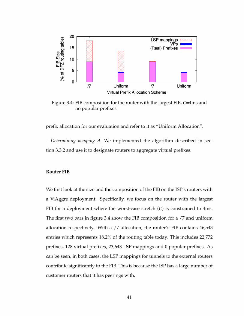
0

5

10

15

20

Uniform/7Uniform/7

FIB

Siz

e(%

of

DF

Z r

ou

tin

g t

ab

le)

Virtual Prefix Allocation Scheme

LSP mappingsVPs

(Real) Prefixes

0

5

10

15

20

Uniform/7Uniform/7

FIB

Siz

e(%

of

DF

Z r

ou

tin

g t

ab

le)

Virtual Prefix Allocation Scheme

LSP mappingsVPs

(Real) Prefixes

Figure 3.4: FIB composition for the router with the largest FIB, C=4ms andno popular prefixes.

prefix allocation for our evaluation and refer to it as “Uniform Allocation”.

– Determining mapping A. We implemented the algorithm described in sec-

tion 3.3.2 and use it to designate routers to aggregate virtual prefixes.

Router FIB

We first look at the size and the composition of the FIB on the ISP’s routers with

a ViAggre deployment. Specifically, we focus on the router with the largest

FIB for a deployment where the worst-case stretch (C) is constrained to 4ms.

The first two bars in figure 3.4 show the FIB composition for a /7 and uniform

allocation respectively. With a /7 allocation, the router’s FIB contains 46,543

entries which represents 18.2% of the routing table today. This includes 22,772

prefixes, 128 virtual prefixes, 23,643 LSP mappings and 0 popular prefixes. As

can be seen, in both cases, the LSP mappings for tunnels to the external routers

contribute significantly to the FIB. This is because the ISP has a large number of

customer routers that it has peerings with.

41

However, we also note that customer ISPs do not advertise the full routing

table to their provider. Hence, edge routers of the ISP could maintain routes

advertised by customer routers in their FIB, advertise these routes onwardswith

themselves as the BGP NEXT HOP and only initiate LSP advertisements for

themselves and for peer and provider routers connected to them. With such a

scheme, the number of LSP mappings that the ISP’s routers need to maintain

and the MPLS overhead in general reduces significantly. The latter set of bars

in Figure 3.4 shows the FIB composition with such a deployment for the router

with the largest FIB. For the /7 allocation, the Worst FIB size is 23,101 entries

(9.02% of today’s routing table), while for the Uniform allocation, it is 10,226

entries (4.47%). In the rest of this section, we assume this model of deployment.

Stretch Vs. FIB Size

We ran the assignment algorithm with Worst Stretch Constraint (C) ranging

from 0 to 10 ms and determined the (Average andWorst) Stretch and FIB Size of

the resulting ViAggre deployment. Figure 3.5(a) plots these metrics for the /7

allocation. The Worst FIB size, shown as a fraction of the DFZ routing table size

today, expectedly reduces as the constraint on Worst Stretch is relaxed. How-

ever, beyond C=4ms, the Worst FIB Size remains constant. This is because the

largest virtual prefix with a /7 allocation encompasses 8.9% of the DFZ routing

table and the Worst FIB Size cannot be any less than 9.02% (0.12% overhead is

due to virtual prefixes and LSP mappings). Figure 3.5(b) plots the same metrics

for the Uniform allocation and shows that the FIB can be shrunk even more.

The figure also shows that the Average FIB Size and the Average stretch are ex-

pectedly small throughout. The anomaly beyond C=8 ms in figure 3.5(b) results

42

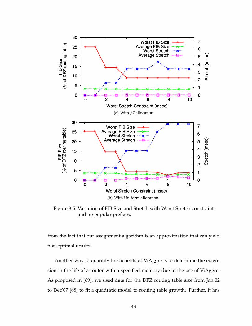
0

5

10

15

20

25

30

0 2 4 6 8 10 0

1

2

3

4

5

6

7

FIB

Siz

e

(%

of

DF

Z r

ou

tin

g t

ab

le)

Str

etc

h (

mse

c)

Worst Stretch Constraint (msec)

Worst FIB SizeAverage FIB Size

Worst StretchAverage Stretch

0

5

10

15

20

25

30

0 2 4 6 8 10 0

1

2

3

4

5

6

7

FIB

Siz

e

(%

of

DF

Z r

ou

tin

g t

ab

le)

Str

etc

h (

mse

c)




(a) With /7 allocation

0

5

10

15

20

25

30

0 2 4 6 8 10 0

1

2

3

4

5

6

7

FIB

Siz

e

(%

of

DF

Z r

ou

tin

g t

ab

le)

Str

etc

h (

mse

c)




0

5

10

15

20

25

30

0 2 4 6 8 10 0

1

2

3

4

5

6

7

FIB

Siz

e

(%

of

DF

Z r

ou

tin

g t

ab

le)

Str

etc

h (

mse

c)




(b) With Uniform allocation

Figure 3.5: Variation of FIB Size and Stretch with Worst Stretch constraintand no popular prefixes.

from the fact that our assignment algorithm is an approximation that can yield

non-optimal results.

Another way to quantify the benefits of ViAggre is to determine the exten-

sion in the life of a router with a specified memory due to the use of ViAggre.

As proposed in [69], we used data for the DFZ routing table size from Jan’02

to Dec’07 [68] to fit a quadratic model to routing table growth. Further, it has

43

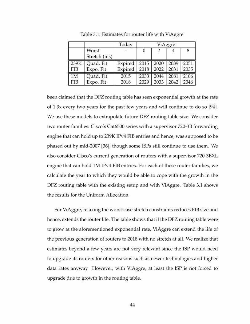
Table 3.1: Estimates for router life with ViAggre

Today ViAggreWorst – 0 2 4 8Stretch (ms)

239K Quad. Fit Expired 2015 2020 2039 2051FIB Expo. Fit Expired 2018 2022 2031 2035

1M Quad. Fit 2015 2033 2044 2081 2106FIB Expo. Fit 2018 2029 2033 2042 2046

been claimed that the DFZ routing table has seen exponential growth at the rate

of 1.3x every two years for the past few years and will continue to do so [94].

We use these models to extrapolate future DFZ routing table size. We consider

two router families: Cisco’s Cat6500 series with a supervisor 720-3B forwarding

engine that can hold up to 239K IPv4 FIB entries and hence, was supposed to be

phased out by mid-2007 [36], though some ISPs still continue to use them. We

also consider Cisco’s current generation of routers with a supervisor 720-3BXL

engine that can hold 1M IPv4 FIB entries. For each of these router families, we

calculate the year to which they would be able to cope with the growth in the

DFZ routing table with the existing setup and with ViAggre. Table 3.1 shows

the results for the Uniform Allocation.

For ViAggre, relaxing the worst-case stretch constraints reduces FIB size and

hence, extends the router life. The table shows that if the DFZ routing table were

to grow at the aforementioned exponential rate, ViAggre can extend the life of

the previous generation of routers to 2018 with no stretch at all. We realize that

estimates beyond a few years are not very relevant since the ISP would need

to upgrade its routers for other reasons such as newer technologies and higher

data rates anyway. However, with ViAggre, at least the ISP is not forced to

upgrade due to growth in the routing table.

44

0.001

0.01

0.1

1

10

100

0 2 4 6 8 10 0

10

20

30

40

50

% o

f T

raff

ic S

tre

tch

ed

a

nd

Im

pa

cte

d

Lo

ad

In

cre

ase

(%

)

Worst Stretch Constraint C (msec)

Traffic StretchedTraffic Impacted

Median Load Increase 0.001

0.01

0.1

1

10

100

0 2 4 6 8 10 0

10

20

30

40

50

% o

f T

raff

ic S

tre

tch

ed

a

nd

Im

pa

cte

d

Lo

ad

In

cre

ase

(%

)

Worst Stretch Constraint C (msec)

Traffic StretchedTraffic Impacted

Median Load Increase

Figure 3.6: Variation of the percentage of traffic stretched/impacted andload increase across routers with Worst Stretch Constraint(Uniform Allocation) and no popular prefixes.

Figure 3.6 plots the impact of ViAggre on the ISP’s traffic and router load.

The percentage of traffic stretched is small, less than 1% for C ≤ 6 ms. This

shows that almost all the traffic is routed through an aggregation point in the

same PoP as the ingress. However, the fact that no prefixes are considered pop-

ular implies that almost all the traffic follows a different router-level path as

compared to the status quo. This shows up in figure 3.6 since the traffic im-

pacted is ≈100% throughout. This, in turn, results in a median increase in load

across the routers by ≈39%. In the next section we discuss how an ISP can use

the skewed distribution of traffic to address the load concern while maintaining

a small FIB on its routers.

Popular Prefixes

Past studies of ISP traffic patterns from as early as 1999 have observed

that a small fraction of Internet prefixes carry a large majority of ISP traf-

fic [42,48,108,127]. We used Netflow records collected across the routers of the

same tier-1 ISP as in the last section for a period of two months (20th Nov’07

45

to 20th Jan’07) to generate per-prefix traffic statistics and observed that this pat-

tern continues to the present day. The line labeled “Day-based, ISP-wide” in

figure 3.7 plots the average fraction of the ISP’s traffic destined to a given frac-

tion of popular prefixes when the set of popular prefixes is calculated across the

ISP on a daily basis. The figure shows that 1.5% of most popular prefixes carry

75.5% of the traffic while 5% of the prefixes carry 90.2% of the traffic.

ViAggre exploits the notion of prefix popularity to reduce its impact on the

ISP’s traffic. However, the ISP’s routers need not consider the same set of pre-

fixes as popular; instead the popular prefixes can be chosen per-PoP or even per-

router. We calculated the fraction of traffic carried by popular prefixes, when

popularity is calculated separately for each PoP on a daily basis. This is plotted

in the figure as “Day-based, per-PoP” and the fractions are even higher. 3

When using prefix popularity for router configuration, it would be prefer-

able to be able to calculate the popular prefixes over a week, month, or even

longer durations. The line labeled “Estimate, per-PoP” in the figure shows the

amount of traffic carried to prefixes that are popular on a given day over the pe-

riod of the next month, averaged over each day in the first month of our study.

As can be seen, the estimate based on prefixes popular on any given day car-

ries just a little less traffic as when the prefix popularity is calculated daily. This

suggests that prefix popularity is stable enough for ViAggre configuration and

the ISP can use the prefixes that are popular on a given day for a month or so.

However, we admit that that these results are very preliminary and we need to

study ISP traffic patterns over a longer period to substantiate the claims made

above.

3We did not have Netflow records for individual routers and hence, were unable to generaterouter-specific popular prefixes.

46

60 65 70 75 80 85 90 95

100

2015105321

% o

f T

raffic

Carr

ied

% of Popular Prefixes

Day-based, ISP-wideDay-based, per-PoP

Estimate, per-PoP

60 65 70 75 80 85 90 95

100

2015105321

% o

f T

raffic

Carr

ied


Day-based, ISP-wideDay-based, per-PoP

Estimate, per-PoP

Figure 3.7: Popular prefixes carry a large fraction of the ISP’s traffic.

Load Analysis

We now consider the impact of a ViAggre deployment involving popular pre-

fixes, i.e. the ISP populates the FIB on its routers with popular prefixes. Specif-

ically, we focus on a deployment wherein the aggregation points are assigned

to constrain Worst Stretch to 4ms, i.e. C = 4ms. Figure 3.8 shows how the traf-

fic impacted and the quartiles for the load increase vary with the percentage of

popular prefixes for both allocations. Note that using popular prefixes increases

the router FIB size by the number of prefixes considered popular and thus, the

upper X-axis in the figure shows the Worst FIB size. The large fraction of traf-

fic carried by popular prefixes implies that both the traffic impacted and the

load increase drops sharply even when a small fraction of prefixes is considered

popular. For instance, with 2% popular prefixes in case of the uniform alloca-

tion (figure 3.8(b)), 7% of the traffic follows a different router-level path than

before while the largest load increase is 3.1% of the original router load. With

5% popular prefixes, the largest load increase is 1.38%. Note that the more even

47

100

10

1

0.1

20151053210

100

31.3

10

1

0.1

2924191412109

% o

f T

raffic

Im

pacte

d

Load Incre

ase

(% o

f native load)


Worst FIB size (% of DFZ routing table)

Traffic ImpactedIncreased Load Quartiles

100

10

1

0.1

20151053210

100

31.3

10

1

0.1

2924191412109

% o

f T

raffic

Im

pacte

d

Load Incre

ase

(% o

f native load)




(a) With /7 allocation

100

10

1

0.1

20151053210

100 39

10

1

0.1

24.519.514.59.56.54.5

% o

f T

raffic

Im

pacte

d

Load Incre

ase

(% o

f native load)




100

10

1

0.1

20151053210

100 39

10

1

0.1

24.519.514.59.56.54.5

% o

f T

raffic

Im

pacte

d

Load Incre

ase

(% o

f native load)




(b) With Uniform allocation

Figure 3.8: Variation of Traffic Impacted and Load Increase (0-25-50-75-100percentile) with percentage of popular prefixes, C=4ms.

distribution of prefixes across virtual prefixes in the uniform allocation results in

a more even distribution of the excess traffic load across the ISP’s routers – this

shows up in the load quartiles being much smaller in figure 3.8(b) as compared

to the ones in figure 3.8(a).

48

2 4 6 8

10 12 14 16 18 20

ATTAbove--net

VSNLExodusGXTiscaliNTTEboneSprintTelstra

FIB

Siz

e(%

of D

FZ

routing table

)

ISP

AverageWorst

2 4 6 8

10 12 14 16 18 20

ATTAbove--net

VSNLExodusGXTiscaliNTTEboneSprintTelstra

FIB

Siz

e(%

of D

FZ

routing table

)

ISP

AverageWorst

Figure 3.9: FIB size for various ISPs using ViAggre.

3.4.3 Rocketfuel Study

We studied the topologies of 10 ISPs collected as part of the Rocketfuel

project [118] to determine the FIB size savings that ViAggre would yield. Note

that the fact we don’t have traffic matrices for these ISPs implies that we can-

not analyze the load increase across their routers. For each ISP, we used the

assignment algorithm to determine the worst FIB size resulting from a ViAggre

deployment where the worst stretch is limited to 5ms. Figure 3.9 shows that the

worst FIB size is always less than 15% of the DFZ routing table. The FIB size is

relatively higher for NTT and Sprint because they have a global footprint with

a few small PoPs outside their main area of influence. For instance, Sprint has

a few small PoPs in the Asia-Pacific region. The constraint on the worst stretch

implies that in many cases, the traffic from these PoPs cannot be routed to an ag-

gregation point in another PoP and so these PoPs must have aggregation points

for all virtual prefixes. Consequently, the routers in these PoPs end up with a

relatively large FIB. However, the Rocketfuel topologies are not complete and

are missing routers. Hence, while the results presented here are encouraging,

they should be treated as conservative estimates of the savings that ViAggre

49

would yield for these ISPs.

3.4.4 Discussion

The analysis above shows that ViAggre can significantly reduce FIB size. Most

of the ISPs we studied are large tier-1 and tier-2 ISPs. However, smaller tier-2

and tier-3 ISPs are also part of the Internet DFZ. Actually, it is probably more

important for such ISPs to be able to operate without needing to upgrade to the

latest generation of routers. The fact that these ISPs have small PoPs might sug-

gest that ViAggre would not be very beneficial. However, given their small size,

the PoPs of these ISPs are typically geographically close to each other. Hence,

it is possible to use the cumulative FIB space across routers of close-by PoPs

to shrink the FIB substantially. And the use of popular prefixes ensures that

the load increase and the traffic impact is still small. For instance, we analyzed

router topology and routing table data from a regional tier-2 ISP (AS2497) and

found that a ViAggre deployment with worst stretch less than 5ms can shrink

the Worst FIB size to 14.2% of the routing table today.

Further, the fact that such ISPs are not tier-1 ISPs implies they are a customer

of at least one other ISP. Hence, inmany cases, the ISP could substantially shrink

the FIB size on its routers by applying ViAggre to the small number of prefixes

advertised by their customers and peers while using default routes for the rest

of the prefixes.

50

PoP1 PoP2

RR1 RR2

R1(VP1)

R4(VP2)

R2(VP2)

R3(VP1)

AS2 AS3

R5 R6

Figure 3.10: WAIL topology used for our deployment. All routers in thefigure are Cisco 7300s. RR1 and RR2 are route reflectors andare not on the data path. Routers R1 and R3 aggregate virtualprefix VP1 while routers R2 and R4 aggregate VP2.

3.5 Deployment

To verify the claim that ViAggre is a configuration-only solution, we deployed

both ViAggre designs on a small network built on the WAIL testbed [21]. The

test network is shown in figure 3.10 and represents an ISP with two PoPs. Each

PoP has two Cisco 7301 routers and a route reflector.4 For the ViAggre deploy-

ment, we use two virtual prefixes: 0.0.0.0/1 (VP1) and 128.0.0.0/1 (VP2) with

one router in each PoP serving as an aggregation point for each virtual prefix.

Routers R1 and R4 have an external router connected to them and exchange

routes using an eBGP peering. Specifically, router R5 advertises the entire DFZ

routing table and this is, in turn, advertised through the ISP to router R6. We

use OSPF for intra-domain routing. Beyond this, we configure the internal dis-

tribution of BGP routes according to the following three approaches:

1). Status Quo. The routers use a mesh of iBGP peerings to exchange the routes

and hence, each router maintains the entire routing table.

4These are used only for the design-II deployment. We used both a Cisco 7301 and a LinuxPC as a route reflector.

51

2). Design-I. The routers still use a mesh of iBGP peerings to exchange routes.

Beyond this, the routers are configured as follows:

– Virtual Prefixes. Routers advertise the virtual prefix they are aggregating to

their iBGP peers.

– FIB Suppression. Each router only loads the routes that it is aggregating

into its FIB. For instance, router R1 uses an access list to specify that only

routes belonging to VP1, the virtual prefix VP2 itself and any popular prefixes

are loaded into the FIB. A snippet of this access list is shown below.

Snippet 1: Access List Configuration

1: . . .

! R5’s IP address is 198.18.1.200

2: distance 255 198.18.1.200 0.0.0.0 1

! Don’t mark anything inside 0.0.0.0/1

3: access-list 1 deny 0.0.0.0 128.255.255.255

! Don’t mark virtual prefix 128.0.0.0/1

4: access-list 1 deny 0.0.0.0 128.0.0.0

! Don’t mark popular prefix 122.1.1.0/24

5: access-list 1 deny 122.1.1.0 0.0.0.255

! . . . other popular prefixes follow . . .

! Mark the rest with admin distance 255

6: access-list 1 permit any

Here, the distance command on line 2 sets the administrative distance of

all prefixes that are accepted by access list 1 to “255” and these routes are

not loaded by the router into its FIB.

52

– LSPs to external routers. We use MPLS for the tunnels between routers. To

this effect, LDP [9] is enabled on the interfaces of all routers and establishes

LSPs between the routers. Further, each edge router (R1 and R4) initiates a

Downstream Unsolicited tunnel [9] for each external router connected to them

to all their IGP neighbors using LDP. This ensures that packets to an external

router are forwarded using MPLS to the edge router which strips the MPLS

header before forwarding them onwards.

Given this setup and assuming no popular prefixes, routers R1 and R3 store

40.9% of today’s routing table (107,943 prefixes that are in VP1) while R2 and R4

store 59.1%.

3). Design-II. The routers in a PoP peer with the route reflector of the PoP

and the route reflectors peer with each other. External routers R1 and R6 are

reconfigured to have eBGP peerings with RR1 and RR2 respectively. The adver-

tisement of virtual prefixes and the MPLS configuration is the same as above.

Beyond this, the route reflectors are configured to ensure that they only adver-

tise the prefixes being aggregated by a router to it. For instance, RR1 uses a

prefix list to ensure that only prefixes belonging to VP1, virtual prefix VP2

itself and popular prefixes are advertised to router R1. The structure of this

prefix list is similar to the access list shown above. Finally, route reflectors use

a route-map on their eBGP peerings to change the BGP NEXT HOP of the ad-

vertised routes to the edge router that the external peer is connected too. This

ensures that the packets don’t actually flow through the route reflectors.

53

3.5.1 Configuration Overhead

A drawback of ViAggre being a “configuration-only” approach is the overhead

that the extra configuration entails. The discussion above details the extra con-

figuration that routers need to participate in ViAggre. Based on our deploy-

ment, the number of extra configuration lines needed for a router r to be config-

ured according to design-I is given by (rint + rext + 2|A(r)| + |Pr | + 6) where rint is

the number of router interfaces, rext is the number of external routers r is peer-

ing with, |A(r)| is the number of virtual prefixes r is aggregating and |Pr| is the

number of popular prefixes in r. Given the size of the routing table today, con-

sidering even a small fraction of prefixes as popular would cause the expression

to be dominated by |Pr | and can represent a large number of configuration lines.

However, quantifying the extra configuration lines does not paint the com-

plete picture since given a list of popular prefixes, it is trivial to generate an

access or prefix list that would allow them. To illustrate this, we developed a

configuration tool as part of our deployment effort. The tool is 334 line Python

script which takes as input a router’s existing configuration file, the list of vir-

tual prefixes, the router’s (or representative) Netflow records and the percent-

age of prefixes to be considered popular. The tool extracts relevant information,

such as information about the router’s interfaces and peerings, from the con-

figuration file. It also uses the Netflow records to determine the list of prefixes

to be considered popular. Based on these extracted details, the script generates

a configuration file that allows the router to operate as a ViAggre router. We

have been using this tool for experiments with our deployment. Further, we

use clogin [151] to automatically load the generated ViAggre configuration file

onto the router. Thus, we can reconfigure our testbed from status quo operation

54

to ViAggre operation (design-I and design II) in an automated fashion. While

our tool is specific to the router vendor and other technologies in our deploy-

ment, its simplicity and our experience with it lends evidence to the argument

that ViAggre offers a good trade-off between the configuration overhead and

increased routing scalability.

3.5.2 Control Plane Overhead

Section 3.4 evaluated the impact of ViAggre on the ISP’s data plane – the impact

on the ISP’s traffic and the routers forwarding this traffic. Beyond this, ViAggre

uses control plane mechanisms to divide the routing table amongst the ISP’s

routers. Design-I uses access lists on routers to suppress routes from be-

ing loaded into the FIB and Design-II uses prefix lists on route reflectors

to prevent the routes from being advertised to their clients, i.e., the routers in

the PoP. We quantify the performance overhead imposed by these mechanisms

using our deployment. Specifically, we look at the impact of our designs on the

propagation of routes through the ISP.

To this effect, we configured the internal distribution of BGP routes in our

testbed according to the three approaches described above. External router R5

is configured to advertise a variable number of prefixes through its eBGP peer-

ing. We restart this peering on router R5 and measure the time it takes for the

routes to be installed into the FIB of the ISP’s routers and then advertised on-

wards; hereon we refer to this as the installation time. During this time, we also

measure the CPU utilization on the routers. We achieve this by using a clogin

script to execute the “show process cpu” command on each router every 5 sec-

55

100

1000

0 50 100 150 200 250

Insta

llatio

n T

ime

(se

c)

Number of Prefixes Advertised (thousands)

Design-I, 2% PPDesign-I, 5% PPDesign-II, 2% PPDesign-II, 5% PP

Status Quo

Figure 3.11: Installation time with different approaches and varying frac-tion of Popular Prefixes (PP).

onds. The command gives the average CPU utilization of individual processes

on the router over the past 5 seconds and we extract the CPU utilization of the

“BGP router” process.

We measured the installation time and the CPU utilization for the three ap-

proaches. For status quo and design-I, we focus on the measurements for router

R1 while for design-II, we focus on the measurements for route reflector RR1.

We also varied the number of popular prefixes. Here we present results with

2% and 5% popular prefixes. Figures 3.11 and 3.12 plot the installation time and

the quartiles for the CPU utilization respectively.

Design-I versus Status Quo. Figure 3.11 shows that the installation time with

design-I is much higher than that with status quo. For instance, with status quo,

the complete routing table is transferred and installed on router R1 in 273 sec-

onds while with design-I and 2% popular prefixes, it takes 487 seconds. Further,

the design-I installation time increases significantly as the number of popular

prefixes increases. Finally, figures 3.12(b) and 3.12(c) show that design-I leads

to a very high CPU load during the transfer, which increases as more prefixes

56

0

20

40

60

80

100

0 50 100 150 200 250C

PU

Utiliz

ation (

%)

Number of Prefixes (thousands)

(a) Status Quo, Measured on R1

0

20

40

60

80

100

0 50 100 150 200 250

CP

U U

tiliz

ation (

%)


(b) Design-I, 2% PP, Measured on R1

0

20

40

60

80

100

0 50 100 150 200 250

CP

U U

tiliz

ation (

%)


(c) Design-I, 5% PP, Measured on R1

0

20

40

60

80

100

0 50 100 150 200 250

CP

U U

tiliz

ation (

%)


(d) Design-II, 2% PP, Measured on RR1

0

20

40

60

80

100

0 50 100 150 200 250

CP

U U

tiliz

ation (

%)


(e) Design-II, 5% PP, Measured on RR1

Figure 3.12: CPU Utilization quartiles (0-25-50-75-100 percentile) for thethree approaches and different fraction of Popular Prefixes(PP).

57

are considered popular. This results from the fact that access lists with a large

number of rules are very inefficient and would obviously be unacceptable for

an ISP deploying ViAggre. We are currently exploring ways to achieve FIB sup-

pression without the use of access list.

Design-II versus Status Quo. Figure 3.11 shows that the time to transfer, in-

stall and propagate routes with design-II is lesser than status quo. For instance,

design-II with 2% popular prefixes leads to an installation time of 124 seconds

for the entire routing table as compared to 273 seconds for status quo. Fur-

ther, the installation time does not change much as the fraction of popular pre-

fixes increases. Figures 3.12(d) and 3.12(e) show that the CPU utilization is low

with median utilization being less than 20%. Note that the utilization shown for

design-II was measured on route reflector RR1 which has fewer peerings than

router R1 in status quo. This explains the fact that the utilization with design-II

is less than status quo. While preliminary, this experiment suggests that design-

II can also help with route convergence within the ISP.

3.5.3 Failover

As detailed in section 3.2.5, as long as alternate aggregation points exist, traffic

in a ViAggre network is automatically rerouted upon failure of the aggregation

point being used. We measured this failover time using our testbed. In the in-

terest of space, we very briefly summarize the experiment here. We generated

UDP traffic between PCs connected to routers R5 and R6 (figure 3.10) and then

crashed the router being used as the aggregation point for the traffic. We mea-

sured the time it takes for traffic to be rerouted over 10 runs with each design.

58

In both cases, the maximum observed failover time was 200 us. This shows that

our designs ensure fast failover between aggregation points.

3.6 Discussion

Pros. ViAggre can be incrementally deployed by an ISP since it does not require the

cooperation of other ISPs and router vendors. The ISP does not need to change

the structure of its PoPs or its topology. What’s more, an ISP could experiment

with ViAggre on a limited scale (a few virtual prefixes or a limited number of

PoPs) to gain experience and comfort before expanding its deployment. None

of the attributes in the BGP routes advertised by the ISP to its neighbors are

changed due to the adoption of ViAggre. Also, the use of ViAggre by the ISP

does not restrict its routing policies and route selection. Further, at least for

design-II, control plane processing is reduced. Finally, there is incentive for de-

ployment since the ISP improves its own capability to deal with routing table

growth.

Management Overhead. As detailed in section 3.5.1, ViAggre requires extra

configuration on the ISP’s routers. Beyond this, the ISP needs to make a number

of deployment decisions such as choosing the virtual prefixes to use, deciding

where to keep aggregation points for each virtual prefix, and so on. Apart from

such one-time or infrequent decisions, ViAggre may also influence very impor-

tant aspects of the ISP’s day-to-day operation such as maintenance, debugging,

etc. All this leads to increased complexity and there is a cost associated with the

extra management.

In section 3.5.1 we discussed a configuration tool that automates ViAggre

59

configuration. We are also implementing a planning tool that takes as input

high-level constraints specified by the human ISP manager such as constraints

on the traffic stretch, router load, router memory used and the robustness of the

resulting design. It then uses ILP to solve a multiple-constraint optimization

problem to generate VA-specific deployment details such as the assignment of

aggregation points. These two tools combined would provide human ISP man-

agers an automated means to adopt ViAggre without needing to delve into Vi-

Aggre and configuration-specific details.

It is difficult to speculate about actual costs, so we do not compare the in-

crease in management costs against the cost of upgrading routers, which apart

from capital costs requires reconfiguring every customer on every router twice.

While we hope that our tools will actually lead to cost savings for a ViAggre

network, an ISP might be inclined to adopt ViAggre just because it breaks the

dependency of various aspects of its operation on the size of the routing table.

These aspects include its upgrade cycle, the per-byte forwarding cost, and the

per-byte forwarding power.

Tunneling Overhead. An important concern arising out of the use of ViAggre

is the tunneling overhead. However, the extensive use of tunnels (MPLS, GRE-

IP, IPSec, VLAN tunneling) in ISP networks has meant that most routers are

already equippedwith interfaces that have extensive tunneling and detunneling

capabilities at line rates [50].

Popular Prefixes. As mentioned earlier, ViAggre represents a trade-off between

FIB shrinkage on one hand and increased router load and traffic stretch on the

other. The fact that Internet traffic follows a power-law distribution makes this

a very beneficial trade-off. This power-law observation has held up in measure-

60

ment studies from 1999 [42] to 2008 (in this thesis) and hence, Internet traffic has

followed this distribution for at least the past nine years in spite of the rise in

popularity of P2P and video streaming. We believe that, more likely than not,

future Internet traffic will be power-law distributed and hence, ViAggre will

represent a good trade-off for ISPs.

Other design points. The ViAggre proposal presented here represents one point

in the design space that we focused on for the sake of concreteness. The ba-

sic idea of dividing the routing table such that individual routers only need to

maintain part of the routes can be achieved using a few alternative approaches.

– Adding routers. We have presented a couple of techniques that ensure that

only a subset of the routing table is loaded into the FIB. Given this, an ISP could

install “slow-fat routers”, low-end devices (or maybe even a stack of software

routers [55]) in each PoP that are only responsible for routing traffic destined to

unpopular prefixes. These devices forward a low volume of traffic, so it would

be easier and cheaper to hold the entire routing table. The popular prefixes are

loaded into existing routers. This approach can be seen as a variant of route

caching and does away with a lot of deployment complexity. In fact, ViAggre

may allow us to revisit route caching [79].

– Router changes. Routers can be changed to be ViAggre-aware and hence, make

virtual prefixes first-class network objects. This would do away with a lot of

the configuration complexity that ViAggre entails, ensure that ISPs get vendor

support and hence, make it more palatable for ISPs. We, in cooperation with a

router vendor, are exploring this option [52].

Routers today tend to have multiple blades with each blade maintaining its

61

own copy of the entire routing table. Another approach involving vendor sup-

port is to split the routing table amongst router blades using ViAggre and hence,

achieve FIB shrinkage with less burden on the ISP itself.

– Clean-slate ViAggre. The basic concept of virtual networks can be applied in an

inter-domain fashion. The idea here is to use cooperation amongst ISPs to in-

duce a routing hierarchy that is more aggregatable and hence, can accrue bene-

fits beyond shrinking the router FIB. This involves virtual networks for individ-

ual virtual prefixes spanning domains such that even the RIB on a router only

contains the prefixes it is responsible for. This would reduce both the router FIB

and RIB and in general, improve routing scalability.

3.7 Related Work

A number of efforts have tried to directly tackle the routing scalability prob-

lem through clean-slate designs. One set of approaches try to reduce rout-

ing table size by dividing edge networks and ISPs into separate address

spaces [38,43,92,100,138]. Our work resembles some aspects of CRIO [138],

which uses virtual prefixes and tunneling to decouple network topology from

addressing. However, CRIO requires adoption by all provider networks and

like other proposals [38,43,92,100], requires a newmapping service to determine

tunnel endpoints. APT [70] presents such a mapping service. Similar to CRIO,

Verkaik et. al. [129] group prefixes with similar behavior into policy atoms and

use these atoms and tunneling of packets to reduce routing table size. Alterna-

tively, it is possible to encode location information into IP addresses [37,51,61]

and hence, reduce routing table size. Finally, an interesting set of approaches

62

that trade-off stretch for routing table size are Compact Routing algorithms; the

key idea behind such algorithms is the adoption of a more flexible notion of

best path. Krioukov et. al. [83] analyze the performance of such an algorithm

for Internet-like graphs; see [84] for a survey of the area.

The use of tunnels has long been proposed as a routing scaling mechanism.

VPN technologies such as BGP-MPLS VPNs [40] use tunnels to ensure that only

PE routers directly connected to the VPN’ed customers need to keep the VPN

routes. As a matter of fact, ISPs can and probably do use tunneling protocols

such as MPLS and RSVP-TE to engineer a BGP-free core [113]. However, edge

routers still need to keep the full FIB. With ViAggre, none of the routers on

the data-path need to maintain the full FIB. Forgetful routing [72] selectively

discards alternative routes to reduce RIB size.

Router vendors, if willing, can use a number of techniques to reduce the

FIB size. This includes FIB compression [113], in which routers don’t install

redundant more-specific prefixes in the FIB. Another technique is route caching

but it seems to have lost favor with both router vendors and ISPs [113].

Another major problem for ISPs with regards to routing scalability is VPN

routing tables. While these tables are only kept by the Provider-Equipment (PE)

routers directly connected to customers need to keep them, they can be several

times larger. In recent work, Kim et. al. [80] use relaying, similar to ViAggre’s

use of aggregation points, to address the VPN routing scalability problem. The

VPN setting involves VPN-specific routing tables and the task of maintaining

these can be split amongst PE routers; in our setting there is just the Internet

routing table and we use the concept of virtual prefixes to make it divisible.

We also have the additional challenge of dealing with networks other than cus-

63

tomers since these networks might be advertising the full routing table, which

is solved by not installing some routes in the FIB (design-I) or through the use

filters on route reflectors (design-II).

Over the years, several articles have documented the existing state of inter-

domain routing and delineated requirements for the future [35,45,89]; see [45]

for other routing related proposals. While scalability might be the most impor-

tant problem afflicting inter-domain routing, several aspects of routing, such

as improving BGP convergence time [124,126], enabling host control over rout-

ing [135], and improving routing security [77,122] have also received a lot of

attention. Mao et al. [89] discuss other such challenges facing the routing sys-

tem.

RCP [25] and 4D [56] argue for logical centralization of routing in ISPs to

provide scalable internal route distribution and a simplified control plane re-

spectively. We note that ViAggre fits well into these alternative routing models

since the centralized control plane can be used to ensure that routers only obtain

the relevant part of the routing table while the data-plane design is the same as

proposed here. As a matter of fact, the use of route reflectors in design-II is

similar in spirit to RCSs in [25] and DEs in [56].

3.8 Summary

In this chapter we presented ViAggre, a technique that can be used by an ISP

to substantially shrink the FIB on its routers and hence, extend the lifetime of

its installed router base. The ISP may have to upgrade the routers for other

reasons but at least it is not driven by DFZ growth over which it has no control.

64

While it remains to be seen whether the use of automated tools to configure

and manage large ViAggre deployments can offset the complexity concerns, we

believe that the simplicity of the proposal and its possible short-term impact on

routing scalability suggest that is an alternative worth considering.

65

CHAPTER 4

IP ANYCASTMEASUREMENT STUDY

4.1 Overview

IP Anycast [102] is an IP addressing and delivery mode whereby an IP packet

is sent to one of a group of hosts identified by the IP Anycast address, typically

the closest one. While IP unicast is one-to-one, and IP Multicast is one-to-many,

IP Anycast is one-to-any.

IP Anycast offers an attractive primitive for service discovery – the route-

to-closest-server abstraction offers reduced access latency for clients, load bal-

ancing across servers, and network-level resilience to DDoS attacks while its

implementation at the network layer allows these advantages to be realized

with no special configuration at clients or servers and with no dependence on

higher-layer services such as the DNS. While this potential has long been rec-

ognized [22,93,102], it is mostly in recent years that IP Anycast has gained in

importance. This is in large part due to its use in the critical DNS root server de-

ployment – six of the thirteen DNS root servers have been transparently repli-

cated using IP Anycast and this deployment continues to grow [63]. In ad-

dition IP Anycast is being used in a variety of other infrastructure services.

For example, IP Anycast is used to improve the performance of caching DNS

servers [95], for drawing in private address space DNS queries as part of the

AS-112 project [140], to discover rendezvous points for multicast groups [81], as

a transition mechanism from IPv4 to IPv6 [67], for sinkholing DoS attacks [57]

and for redirection in commercial CDNs [141]. Finally, recent research efforts

include renewed interest in the use of IP Anycast for CDNs [7] and a proposal

66

for its use as a vehicle for next-generation architecture deployment [12,105].

However, despite its growing use in critical infrastructure services, IP Any-

cast and its interaction with IP routing practices is not well understood. A cou-

ple of root server operators [20,33] have offered valuable reports on the perfor-

mance of their anycast deployments. These are probably the first reports on the

performance of IP Anycast and represent the best source of data on operational

IP Anycast deployments from the point of view of the anycast servers. How-

ever, the analysis is preliminary (as the authors themselves state) and details of

the study are not published, nor is the data publicly available. Drawing from

these, in this chapter we present a detailed study of inter-domain IP Anycast as

measured from a large number of vantage points. Specifically, our study seeks

to answer the following questions:

1. What kind failover properties does a typical IP Anycast deployment offer?

2. What kind of load distribution do existing IP Anycast deployments see?

Also, can the operator of an anycast deployment control this distribution

of client load?

3. Past studies [112] have reported that existing IP Anycast deployments

may offer poor latency-based proximity; i.e., many clients may not be

routed to the server closest in terms of latency. Using a larger number of

clients and anycast groups, we aim to confirm and understand the reasons

for this poor latency as well as explore possible remedial measures.

4. Past studies [20,24,33,111] have presented conflicting reports regarding the

affinity offered by IP Anycast and consequently, the ability to run stateful

67

services of top of anycast.1 We seek to measure, at scale, the affinity offered

by IP Anycast.

To explore these questions, we study four existing IP Anycast deployments in-

cluding two anycasted DNS root servers. In terms of methodology, our study

differs from previous efforts on two fronts:

1. We use a variant of the King [59] measurement technique to observe and

evaluate IP Anycast deployments from a very large number (>20,000) of

vantage points. To the best of our knowledge, this represents a two or-

der of magnitude increase in the number of vantage points from which IP

Anycast deployments have been actively probed for evaluation.

2. We deploy our own small scale IP Anycast service for controlled evalu-

ation of anycast under different deployment and failure scenarios. Per-

forming such experiments would be difficult using commercial IP Anycast

deployments such as the DNS root servers.

The main results of this study are as follows:

• We corroborate evidence from past studies indicating that IP Anycast, by

itself, does not offer good latency-based proximity. For example, for the 13

server J-root deployment, we find that 8903 (≈40%) of the 22,281measured

clients are directed to a root server that is more than 100 ms farther away

than the closest server. While the impact of inter-domain routing on end-

to-end path length has been well documented [117], we find that inter-

1Affinity measures the extent to which consecutive anycast packets from a client are deliv-ered to the same anycast server.

68

domain routing metrics have an even more severe impact on the selection

of paths to anycast destinations.

• We propose and evaluate a practical deployment scheme designed to al-

leviate the proximity concerns surrounding IP Anycast. Specifically, en-

suring that an ISP that provides transit to an anycast server has global

presence and is (geographically) well covered by such servers improves

the latency-based proximity offered by the anycast deployment.

• We find that IP Anycast is affected by delayed routing convergence and

hence, clients using anycast services may experience slow failover. How-

ever, our proposed deployment scheme addresses this by reducing the

scope of routing convergence that follows a server failure and hence, can

ensure that clients failover at a fast rate. For instance, we find that in case

of a server failure in an IP Anycast deployment conforming to our pro-

posal, a vast majority (>95%) of clients can be rerouted to other operational

servers in less than 20 seconds.

• Ours is a much larger scale study than past efforts. Through this, we find

that the anycasting of an IP prefix does not have any unfavorable interac-

tions with inter-domain routing. Hence, IP Anycast offers very good affin-

ity for all but a very small fraction of clients. Using temporal clustering,

we show that the poor affinity observed by this small fraction of clients

can be attributed to dynamic load balancing mechanisms near them.

• We find that a naive IP Anycast deployment does not lead to an even dis-

tribution of client load across servers. However, we also propose and eval-

uate the impact of operators manipulating BGP advertisements at individ-

ual anycast servers to control their load. Our results show that such mech-

anisms can achieve coarse-grained load balancing across anycast servers.

69

Overall, our measurements show that an IP Anycast service can be deployed so

as to provide a robust substrate offering good proximity and fast failover while

allowing for coarse-grained control over server load. In the rest of this chapter,

we detail our measurement methodology and results. In the next chapter, we

use our insights into how to deploy a native IP Anycast service to guide a new

Anycast architecture that addresses the limitations of native IP Anycast.

4.2 Related Measurement Studies

An invaluable vantage point for measuring anycast deployments is at the any-

cast servers themselves. In recent presentations [20,33], the operators of the J

and K root servers report on their analysis of client logs collected at their any-

cast servers. They present the observed distribution of client load and affinity.

In terms of load distribution, both studies report a skewed distribution of client

load across their respective deployments. With regard to affinity, the J-root op-

erators report instances of clients that exhibit poor affinity and conjecture that

anycast may not be suitable for stateful services. By contrast, the K-root opera-

tors find that most of their clients experience very high affinity.

Our study builds on these earlier reports. Using active measurements from

over 20,000 clients, we measure the affinity and load distribution for our own

small-scale anycast deployment, explore the reasons behind the observed load

and affinity, and evaluate techniques to control server load. In addition to load

and affinity, we use active measurements to evaluate the (latency) proximity

seen at clients to four different anycast deployments. Finally, using our own

deployment, we study the behavior of IP Anycast under server failure. As we

70

describe in Section 4.6, our desire to use a large number of client vantage points

prevents us frommeasuring the affinity and load to the DNS root server deploy-

ments. However, for completeness, we did perform such measurements from

a smaller set of clients that we have direct access to (i.e., PlanetLab nodes [31]

and approximately 200 publicly-available traceroute servers). Since the results

were consistent with the larger-scale measurements over our own deployment,

we only present the latter here. The details of the PlanetLab-based study can be

found in [15].

We are aware of two recent efforts that measure the performance of IP Any-

cast using active probing from clients. Sarat et al. [111,112] use PlanetLab nodes

as vantage points for evaluating the K-root, F-root and .ORG TLD deployments.

They measure proximity and affinity and report poor proximity and moderate-

to-poor affinity. Similarly, using PlanetLab and approximately 200 volunteer

nodes, Boothe et al. [24] measure the affinity offered by the anycasted DNS root

servers and report poor affinity.

4.3 Deployments Measured

An IP Anycast group is associated with an IP address (referred to as the any-

cast address for the group) and servers join the group by just advertising this

address into the routing infrastructure. For an intra-domain anycast group with

servers restricted to a single administrative domain, this advertisement is into

the intra-domain routing protocol for the domain in question. For inter-domain

anycast groups, each server advertises the anycast address into BGP. 2 Despite the

2In practice, each server must advertise a prefix for a block of addresses into BGP. This is theanycast prefix for the group and servers are accessible through all addresses in the prefix.

71

Table 4.1: The three external IP Anycast deployments that we evaluate.

Name Anycast AS# No. ofprefix servers

F root server [145] 192.5.5.0/24 3557 27J root server [148] 192.58.128.0/24 26415 13AS 112 [140] 192.175.48.0/24 112 20

Table 4.2: The internal IP Anycast deployment comprising of five servers. Eachof these advertise the anycast prefix (204.9.168.0/22) through a BGP peeringwith their host-site onto the upstream provider. Note that IR stands for “Intel-Research”.

Server Host-Site Host-site UpstreamUnicast address AS# provider

128.84.154.99 Cornell University 26 WCG12.155.161.153 IR Berkeley 2386 ATT195.212.206.142 IR Cambridge 65476 ATT-World12.108.127.148 IR Pittsburgh 2386 ATT12.17.136.150 IR Seattle 2386 ATT

simplicity of the basic idea, the interaction with BGP, the involvement of mul-

tiple administrative domains etc. raise several interesting questions regarding

the behavior of inter-domain IP Anycast. We restrict ourselves to studying is-

sues related to inter-domain IP Anycast. Also, while we focus on IPv4 Anycast,

our results should apply equally to IPv6 Anycast deployments.

Since clients can access an anycast group simply by sending packets to the

IP address associated with the group, IP Anycast has been used for transparent

replication of many services including the DNS root servers. For example, the

F root server deployment is currently comprised of 37 servers that form an IP

Anycast group and each server advertises the F root server anycast prefix. The

deployment is also associated with its own AS number (AS#) which serves as

the origin AS for the anycast prefix. Thus, clients can access a F root server

by sending packets to an address in the prefix. Here we evaluate three such

72

currently operational deployments - two anycasted DNS root servers and the

AS112 anycast deployment.3 The anycasted AS112 servers are used to draw in

reverse DNS queries to and for the link local address space (RFC1918 addresses–

10.0.0.0/8, 172.16.0.0/12 and 192.168.0.0/16). Since we have no control over

these deployments, we refer to these as external deployments. Table 4.1 gives

details for the external deployments including the number of the servers in each

deployment at the time of our experiments.4

In practice, each “server” in these deployments is a cluster of hosts located

behind some form of load balancing device. For example, for the F root server,

hosts in each cluster form an intra-domain anycast group and it is the server

site’s gateway routers that balance incoming traffic between them [2]. However,

our focus on inter-domain anycast makes our measurements oblivious to this

cluster-based deployment. Thus, for the purpose of our study, each server site

can be thought of as a single host.

The production-mode nature of these external deployments makes it dif-

ficult, if not impossible, to conduct controlled experiments such as injecting

server failure, or manipulating the advertisements at individual servers. For

such experiments we deployed our own IP Anycast service that we call the in-

ternal deployment. For this, we obtained a /22 prefix (204.9.168.0/22) and an

AS# (33207) from ARIN and deployed anycast servers at the five sites listed in

table 4.2. Each server advertises this prefix and AS# into BGP through their

host site and on to their upstream provider and hence they form an IP Anycast

group.

3The choice of the anycast deployment to measure was limited by the need to know theunicast addresses of the individual anycast servers for our experiments.

4All three deployments have since grown substantially.

73

Note that an anycast server’s “host-site” refers to the server’s immediately

upstream ASwhile the “upstream provider” refers to the closest major ISP (tier-

1 or tier-2) that provides transit for the server’s traffic. For example, the internal

deployment anycast server at Cornell has Cornell (AS# 26) as its host-site and

Williams Communication (WCG – AS#7911) as its upstream provider. This dif-

ference between the host-site and upstream provider is a quirk of the internal

deployment; for most commercial IP Anycast deployments, the host-site is also

the upstream provider.

The internal deployment is as yet very small in scale. The biggest hurdle

in growing the deployment has been the site-by-site negotiation with upstream

providers (ATT, WCG) to clear the advertisement of our anycast prefix. Note

that we do not require these upstream providers to actively inject our prefix

in the BGP but only propagate the advertisement from the anycast servers on-

wards. Instead, the approval from the ISPs is only due to the access control ISPs

often enforce on the AS numbers and network prefixes they expect to see adver-

tised from their customers. To accelerate this site-by-site deployment, we are

currently in the process of deploying anycast servers over NLR [146]. Further

details about the internal deployment as well as the requirements for much wel-

come volunteer sites are available at [10]. While the small size of the internal de-

ployment certainly raises questions regarding the generality of our results, the

fact that (in retrospect) most of our results follow intuitive reasoning supports

the applicability of our study.

74

Table 4.3: Geographic distribution of the clients used in our study.

Region No. of clients % of Total

North America 12931 54.827Central America 317 1.344South America 461 1.954

Europe 5585 23.680Asia 2402 10.184

S.E. Asia 566 2.400Oceania 1196 5.071Africa 187 0.792

Arctic Region 9 0.038Unknown 204 0.864

Total 23858 100.000

1

Auckland

Amsterdam

Barcelona

Toronto

Client X

3

2(Recursive

4

1 A? random_no.f-root.anycast.guha.cc

2 NS? f-root.anycast.guha.cc

3 NS(f-root.anycast.guha.cc)

A(f.root-servers.net)=192.5.5.241

4 A? random_no.f-root.anycast.guha.cc

5

5 NXDOMAIN6

6 --same as (5)--

Measurement Host (M)

=f.root-servers.net

(or a pointer to the root-servers)

Nameserver)

F root-server

F root-server

F root-server

F root-server

Figure 4.1: Measurement Host M uses DNS queries to direct client X tosend packets to the anycast address associated with the F rootserver deployment. In the scenario depicted here, packetsfrom X are routed to the anycasted F root server located atAuckland, Australia. Note that we use a domain under ourcontrol (anycast.guha.cc) to trick client X into assumingthat 192.5.5.241 is the authoritative nameserver for the domainf-root.anycast.guha.cc.

75

4.4 Methodology

A key observation guiding our measurement methodology is that all three ex-

ternal deployments are DNS services. Hence, the anycast servers that are part

of these deployments are all DNS nameservers, and we can probe them using

DNS queries. However, since packets from a client to the anycast address of any

given anycast deployment are delivered to one of the servers, a large number

of clients are needed to ensure that we are able to reach all the anycast servers.

To achieve this we used the King measurement technique [59]. King allows for

measurement of latency between any two arbitrary hosts on the Internet by uti-

lizing recursive nameservers near the hosts in question.

Using the same basic idea, we used recursive DNS nameservers in the Inter-

net as clients in our study. To this effect, we took an address in each routable

prefix in a BGP routing table obtained from Route-Views [149] and deter-

mined if any of the nameservers authoritative for the in-addr.arpa name

associated with the address had recursion enabled. For example, for the pre-

fix 128.84.223.0/24, we determined if any of the nameservers authoritative for

the name 1.223.84.128.in-addr.arpa. had recursion enabled. This ap-

proach yielded a list of 23,858 unique recursive nameservers. Table 4.3 details

the geographic distribution of these nameservers. The nameservers belong to

7,566 different ASs. Hence, they provide us a view of the anycast deployments

from 7,566 of the 18,391 routeable ASs on the Internet (based on a BGP routing

table obtained from Route-Views). The quantity and the spread of these name-

servers makes us confident that our measurements closely reflect the behavior

of IP Anycast as seen from hosts in the Internet in general.

76

Note that using a large number of clients yields a more representative pic-

ture for all the metrics we measure here. For example, the scale of our study

makes our arguments regarding client load distribution across the anycast de-

ployment significantly more representative than (say) just using PlanetLab for

measurements. Moreover, our use of widely-dispersed Internet nameservers as

clients avoids the bias that would be introduced were we to use PlanetLab hosts

as clients. This bias could severely impact the affinity, proximity and load mea-

surements. For example, one of the J-root servers is connected to the GEANT

network and hence, can be accessed through Internet2. Consequently, a large

fraction of PlanetLab nodes are routed to this server when they probe the J-root

anycast address.

Evaluating an IP Anycast deployment from the perspective of any client

(say X) in the list requires that we be able to direct X to send packets to the

anycast address of the deployment. As suggested by [59], we leveraged the

fact that X is a recursive nameserver and hence, is willing to resolve DNS

queries on behalf of other hosts. We can thus “trick” client X into sending

DNS queries to an anycast address by making the NS record for a domain point

to the address in question and querying X for any record in that domain. We

used anycast.guha.cc, a domain we own, for this purpose. For example,

in case of the F root server deployment with anycast address 192.5.5.241, we

created a domain f-root.anycast.guha.ccwith its NS record pointing to

192.5.5.241. As illustrated in figure 4.1, querying client X for any record in this

domain (for example, random no.f-root.anycast.guha.cc) causes X to

resolve the NS record for f-root.anycast.guha.cc (packets (2) and (3)),

and then send a query to the anycast address for the F root server deployment

(packet (4)). Aminor practical problemwith this approach is that a client may be

77

configured to resend query (4) a number of times on seeing that the response (5)

is an error. As suggested by [59], we weeded out clients that may resend queries

on receiving an error as follows: we directed each client to the anycast address

of the internal anycast deployment and logged the DNS queries at each of the

servers of the internal deployment to determine the number of times query (4)

is sent.

The experiments presented here use this basic technique for various tasks

such as determining the particular anycast server accessed by each client and

the latency of doing so. For example, to determine the latency from a client X to

the anycast address of the F root server, we:

• Send a recursive DNS query to client X for the NS record for

f-root.anycast.guha.cc: this primes client X’s cache with the fact

that the F root server anycast address corresponds to the authoritative

nameserver for the domain f-root.anycast.guha.cc

• Send an iterative DNS query to client X: since an iterative query is an-

swered by client X based on local information, this provides us with an

estimate of the latency for packets {(1),(6)} in figure 4.1.

• Send a recursive DNS query to client X for the A record for

random no.f-root.anycast.guha.cc: as shown in figure 4.1, this

causes client X to send packets to the F root server anycast address and

provides us with an estimate of the latency for packets {(1), (4), (5), (6)}.

This process is repeated eight times and the difference between the minimum

measured latency for packets {(1), (4), (5), (6)} and {(1), (6)} is used as an esti-

mate of the round-trip anycast latency from client X to the F root server.

78

4.5 Proximity

The value of anycast as a server selection primitive is in part due to its ability

to find close servers. With IP Anycast, packets destined to an anycast address

are routed to the server closest to the client in terms of the metrics used by the

underlying routing protocol. For inter-domain IP Anycast, it is the BGP decision

process (including routing policies) at the various ASs that governs the anycast

server accessed by each client. This implies that anycast packets from clients

may not be delivered to servers that are close in terms of latency and recent

studies [112] have, in fact, indicated that IP Anycast offers poor latency-based

proximity. In this section we use latency measurements from our ≈ 20,000 clients

to show that this is indeed the case for existing anycast deployments. However,

we also argue that poor latency can be avoided through a planned deployment.

Methodology: To determine the quality of proximity offered by an IP Any-

cast deployment to a given client, we need to determine the following latencies:

• Unicast Latency to all anycast servers - here, unicast latency to an anycast

server is the latency from the client to the unicast address of the server.

Given that each client is a recursive nameserver, the King approach for

determining latencies between two hosts applies here directly.

• Anycast Latency for the client or the latency from the client to the anycast

address of the deployment. The procedure for determining the anycast

latency for a client was described in the previous section.

We define stretch-factor as the difference between the anycast latency and

the minimum unicast latency for a client. The stretch factor thus represents

79

0

0.2

0.4

0.6

0.8

1

-50 0 50 100 150 200

CD

F

Difference of Anycast and Minimum Unicast latency (msec)

F RootJ RootAS112

InternalDiff=30msec

0

0.2

0.4

0.6

0.8

1

-50 0 50 100 150 200

CD

F


F RootJ RootAS112

InternalDiff=30msec

Figure 4.2: CDF for the difference between the anycast and minimum uni-cast latency for the external and the internal deployments.

the quality of latency-based proximity an anycast deployment offers a client.

We determined the stretch factor for each client in our list for the external and

internal anycast deployments.

Results: Figure 4.2 shows the CDF for the stretch factor for all the clients.

The stretch factor can be negative because anycast packets may be routed to the

closest server, yet take a path shorter than the unicast path to the closest server.

We see that for all four anycast deployments, a fair fraction of clients are not

routed to the server closest to them.5 For example, the number of clients that

are routed to a server that is more than 30 ms farther away from the closest

server ranges from 31% (for the internal deployment) to 61% (for the AS112 de-

ployment). Similarly, in case of the J root server deployment, 40% of the clients

incur a stretch-factor of more than 100 ms.

5The poor selection in case of F root server deployment can be attributed to their use ofhierarchical anycast [1,145]. In effect, only 2 of the 27 F root servers advertise the F-root anycastprefix globally. So it is not fair to compare the anycast latency to the minimum unicast latencyacross all the 27 servers. However, this is not the case for the other deployments we measured.

80

IP Anycast deployments, by their very nature, are vulnerable to the fact that

Internet routing is not based on latency. This is because the anycast servers

are geographically distributed and hence, there is greater margin for error in

selecting which server to route to. This, in turn, results in the inefficacy of IP

Anycast in selecting closeby anycast servers. The issue is exacerbated by the fact

that anycast servers tend to have different upstream providers, which is true for

both the internal and the external anycast deployments. For example, in case

of the internal deployment, the anycast servers have three different upstream

providers.

The following anecdotal scenario serves to illustrate the causes of poor prox-

imity. We use the example of a publicly available traceroute-server at UC-

Berkeley (net.berkeley.edu) acting as a client trying to access the inter-

nal anycast deployment. Anycast packets from this client are routed to the

server at Cornell (latency=87msec) instead of the close-by server at Berkeley (la-

tency=9msec). Figure 4.3 shows the relevant AS-level connectivity with the rele-

vant POPs of ATT (upstream provider for the server at Berkeley) andWCG (up-

stream provider for the server at Cornell). We used BGP looking-glass servers

to determine that Level3 has at least two paths for the internal deployment’s

anycast prefix: one through WCG’s Santa Clara POP with AS-PATH=[7911, 26,

33207] and the other through ATT’s San Francisco POP with AS-PATH=[7018,

2386, 33207]. The Level3 routers in the area choose the first path as the best path

and hence, anycast packets from the client are delivered to the anycast server at

Cornell. This path is labeled as “Actual Path” in the figure.

This example points to the crux of why Internet routing yields poor prox-

imity for the measured anycast deployments. From the point of view of inter-

81

WCG (7911)

ATT (7018)

UCB

CSUNET

Cornell

(25)

Level3

IR Berk

(2386) Berk

Server

(2152)

(26)

Cornell Server(33207)

(3356)

4

1 2

3

(33207) 1 WCG (SantaClara POP) 2 WCG (NY POP)

3 ATT (SF, CA POP) 4 ATT (NY POP)

X Client

(net.berkeley.edu)

Actual Path Ideal Path

Figure 4.3: The relevant AS-level connectivity (with correspond-ing AS numbers in parenthesis) between the client(net.berkeley.edu) in UC-Berkeley and the internalanycast deployment servers at Cornell and Berkeley. Level3receives at least two different advertisements for the internaldeployment anycast prefix with the following AS-PATHs:[7911, 26, 33207] and [7018, 2386, 33207].

Internal Deployment(AS# 33207)

Cornell Seattle

PittsburghBerkeley

Cambridge

WCG (AS# 7911)

ATT (AS# 7018) ATT -World

(AS# 2686)

Figure 4.4: AS-level connectivity for the anycasted internal deployment –from the point of inter-domain routing, AS# 33207 is a multi-homed stub AS.

82

domain routing, an anycasted AS is equivalent to a multi-homed stub AS (see

figure 4.4). However, anycasting introduces multi-homing scenarios which dif-

fer significantly from normal multi-homing scenarios. In typical multihoming,

multiple peerings of the multihomed stub AS are in the same geographical area.

As a consequence, selection of paths from clients to the multihomed AS based

on ISP policies and AS-PATH length leads to acceptable performance. On the

other hand, for an anycasted AS, the multiple peerings are geographically dis-

persed, but this is not accounted for in the existing inter-domain routing set-up.

In the example above, Level3 receives two paths to the anycasted internal de-

ployment of equal AS-PATH length and is not aware of the actual physical dif-

ference between the length of these paths. Consequently, there is a good chance

that Level3 may choose a route that causes the anycast packets to be routed to a

distant anycast server. In other words, current route selection mechanisms have

a much higher chance of making an unsuitable choice when selecting paths to

an anycasted AS.

Although negative, the importance of this observation cannot be overem-

phasized. It brings to light that while the routing protocols used to choose paths

to unicast destinations work naturally for anycast destinations too, the metrics

used for routing decisions can lead to a poor choice of anycast server in terms

of latency. While changing routing protocols to differentiate between anycast

and unicast prefixes would be one possible approach to address this problem, a

more practical approach would be to plan the deployment of the anycast servers

to account for inter-domain route selection.

We hypothesize that deploying the anycast servers such that all of them have

the same upstream provider and the servers are spread across the provider is

83

Internal Deployment(AS# 33207)

SeattlePittsburgh

Berkeley

ATT

(AS# 7018)

Level3

(AS# 3356) Level3 routers route

anycast packets to an

ATT POP based on

ATT MEDs (’’’late-exit’)

or Level3’s intra-domain

metrics (’’early exit’’)

ATT routers route

anycast packets to the

anycast server closest

in terms on ATT’s

intra-domain metrics

Figure 4.5: Shown here is a deployment with ATT as the common up-stream provider – ASs beyond ATT route the anycast packetsto ATT’s network. Here, Level3’s routers route anycast pack-ets to a close-by ATT POP which then routes the packets to theclosest anycast server.

one such deployment approach. This approach is based on two key observa-

tions. First, an ISP that is an upstream provider for some of the anycast servers

routes incoming anycast traffic to the server closest among them; this is a con-

sequence of the fact intra-domain traffic engineering is mostly consistent with

latency sensitive routing [117]. For example, in case of the internal deployment,

ATT is an upstream provider for three of the five anycast servers. Routers in

ATT’s network receive routes of equal AS-PATH length and equal preference

from each of these anycast servers. Hence, the BGP decision process causes in-

coming anycast packets at any ATT POP to be routed to the server that is closest

in terms of the intra-domain metrics used by ATT. As the measurements pre-

sented next show, this server is also closest in terms of latency in a largemajority

of cases.

Second, such a deployment decouples route selection at the common up-

stream provider from the selection at ASs beyond it. Due to reasons detailed

above, the common upstream provider delivers incoming anycast packets to

84

the closest server. Any ASs farther away from the anycast server sites than

the upstream provider only need to select among the possible routes to the up-

stream provider. Figure 4.5 illustrates this. Of these ASs, the ones that use an

“early-exit” (or hot-potato routing) routing policy would route anycast packets

to the closest POP of the common upstream provider. Alternatively, ASs that

use a “late-exit” (or cold-potato routing) routing policy would honor the MEDs

of the upstream provider and route anycast packets to the upstream provider

POP that is most suitable for delivery to the closest of the deployed anycast

servers. While it is possible that an AS may choose overly long paths to the

upstream provider, the prevalence of the two aforementioned policies amongst

ASs leads us to believe that this would not be the norm and our measurements

confirm this. Its also important to note that any overhead arising due to the

choices made at this step of the selection process also apply to the inter-domain

routing in general and are not specific to anycast per se.

Hence, in case of the internal deployment, we would like to ensure that in-

stead of five servers with three different upstream providers, all the servers

should have the same provider. As a matter of fact, the subset of the internal

deployment comprising of the three servers at Berkeley, Pittsburgh and Seattle

conforms to our deployment proposal. These servers have the same upstream

provider (ATT) and are geographically spread out. With this three server de-

ployment, all anycast packets would be routed to the ATT network and then

delivered byATT to the (closest) anycast server. For instance, if the sample client

(net.berkeley.edu) presented above accessed this deployment, it would be

routed to the server at Berkeley. This is because, in figure 4.3, Level3 would not

receive an advertisement for the anycast prefix from WCG. Instead, Level3’s

routers would route the client’s packets to the ATT POP at San Francisco. The

85

0

0.2

0.4

0.6

0.8

1

-50 0 50 100 150 200

CD

F


AllAll - Cam

All - Cam - CorAll - Pit - BerkDiff.=30msec

0

0.2

0.4

0.6

0.8

1

-50 0 50 100 150 200

CD

F


AllAll - Cam

All - Cam - CorAll - Pit - BerkDiff.=30msec

Figure 4.6: CDF for the difference between the anycast and minimum uni-cast latency for various subsets of the internal deployment.Here, All - x implies measurements with server x switched off.

routers in ATT’s San Francisco POP would in turn route these packets to the

nearest anycast server. Thus, the anycast packets would be routed to the server

at Berkeley and not at Seattle or Pittsburgh. We validated this by stopping the

advertisement of the anycast prefix from the Cornell and the Cambridge server

to remove them from the anycast deployment and observing that the anycasted

packets from the sample client were delivered to the anycast server at Berkeley.

This path is labeled “Ideal Path” in Figure 4.3.

To validate this hypothesis, we repeated the stretch factor measurements for

our list of clients with only subsets of the internal deployment operational. Fig-

ure 4.6 shows the results from these measurements. As can be seen, an any-

cast deployment comprising of just the three servers at Berkeley, Pittsburgh and

Seattle (labeled as “All - Cam - Cor” in the figure) yields good proximity with

just 5% of the clients incurring a stretch factor of more than 30msec. Note that

it may seem that this improvement in the stretch factor for clients is due to the

86

fact that the choice of servers has reduced from five to three. To account for this

we also measured the proximity offered by a deployment with the three servers

at Seattle, Cornell and Cambridge. All these servers have a different upstream

provider and as can be seen from the figure (curve labeled as “All - Pit - Berk”),

this yields poor proximity too. These results show that an anycast deployment

with all servers having the same upstream provider does provide good latency-

based proximity to clients.

As a matter of fact, this result can be generalized. It is possible to have

anycast deployments with multiple upstream providers for the anycast servers.

However, all the upstream providers should have reasonable global geographic

spread (in essence, tier-1 ISPs with a global network) and for each upstream

provider, there must be a sufficient number of servers to cover the geograph-

ical spread of the provider. In such a set-up, whenever any of the upstream

providers receives an anycast packet, there is a close-by anycast server that the

packet can be routed to. ASs beyond these upstream providers would choose

to route the anycast packets to one of the upstream providers and since all the

providers are well covered by the anycast servers, this choice does not have a lot

of bearing on the anycast path length. Due to reasons described earlier, each AS

beyond the upstream providers for the anycast deployment would most likely

route the packets to a suitable POP of the upstream provider it chooses. Thus,

a deployment according to this model would offer good latency based proxim-

ity to clients. The small size of the existing internal deployment does not allow

us to validate this claim; however, this is something that we aim to address in

future work.

87

4.6 Failover time

Inter-domain IP Anycast involves each site advertising the anycast prefix into

BGP. Consequently, when an anycast server fails, the process by which clients

using the failed server are rerouted to other operational servers is tied to BGP

convergence. Past studies have shown that failures at multi-homed end sites

can lead to a convergence process that may last for minutes [86]. Such a slow

failover, if it applies to IP Anycast to, would not bode well for a number of

proposed uses of IP Anycast. Hence we decided to measure the failover rate for

the internal anycast deployment. To the best of our knowledge, this represents

the first attempt to study the failure-mode behavior of IP Anycast.

Methodology: In order to determine the rate at which clients failover when

an anycast server fails, we need to be able to determine the specific anycast

server that each client is routed to. To this effect, we configured the anycast

servers in the internal deployment to act as authoritative nameservers for a

domain under our control (internal.anycast.guha.cc) and to respond to

TXT-type DNS queries for this domain with a location-specific string. For exam-

ple, a TXT-type DNS query for this domain from a client whose anycast packets

are routed to the anycast server at Cornell will receive “Cornell” as the response.

This, when combined with the ability to direct clients to send DNS queries to the

anycast address of the internal deployment, allows us to determine the anycast

server being accessed by all clients in our list. Figure 4.7 illustrates this process

for one client.

The internal deployment servers have been configured to respond to TXT-

type queries with a TTL value of 0. This implies that clients cannot cache the

88

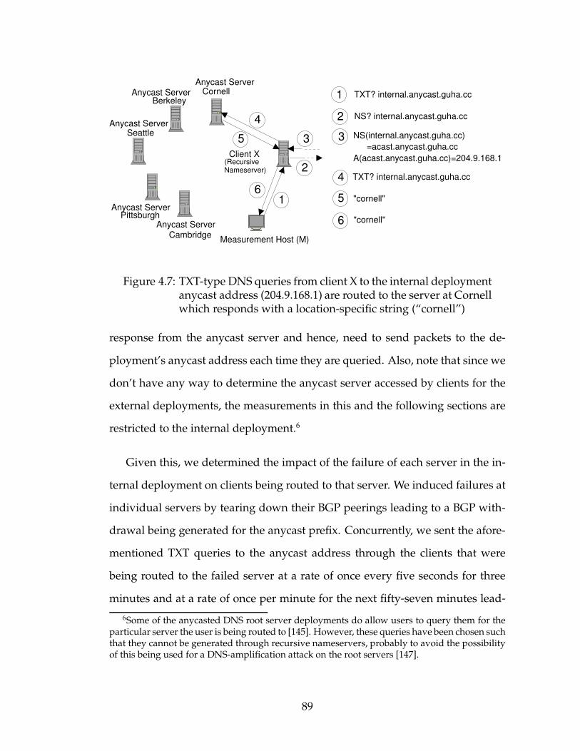
1

CornellBerkeley

Seattle

Cambridge

Client X

3

2(Recursive

4

1 TXT? internal.anycast.guha.cc

2 NS? internal.anycast.guha.cc

3 NS(internal.anycast.guha.cc)

A(acast.anycast.guha.cc)=204.9.168.1

4 TXT? internal.anycast.guha.cc

5

5 "cornell"6

6

Measurement Host (M)

=acast.anycast.guha.cc

Nameserver)

Anycast ServerAnycast Server

Anycast Server

Anycast Server

Anycast ServerPittsburgh

"cornell"

Figure 4.7: TXT-type DNS queries from client X to the internal deploymentanycast address (204.9.168.1) are routed to the server at Cornellwhich responds with a location-specific string (“cornell”)

response from the anycast server and hence, need to send packets to the de-

ployment’s anycast address each time they are queried. Also, note that since we

don’t have any way to determine the anycast server accessed by clients for the

external deployments, the measurements in this and the following sections are

restricted to the internal deployment.6

Given this, we determined the impact of the failure of each server in the in-

ternal deployment on clients being routed to that server. We induced failures at

individual servers by tearing down their BGP peerings leading to a BGP with-

drawal being generated for the anycast prefix. Concurrently, we sent the afore-

mentioned TXT queries to the anycast address through the clients that were

being routed to the failed server at a rate of once every five seconds for three

minutes and at a rate of once per minute for the next fifty-seven minutes lead-

6Some of the anycasted DNS root server deployments do allow users to query them for theparticular server the user is being routed to [145]. However, these queries have been chosen suchthat they cannot be generated through recursive nameservers, probably to avoid the possibilityof this being used for a DNS-amplification attack on the root servers [147].

89

ing to a total probe period of one hour. For each such client, we determined the

time it takes for the client to failover and “settle” at a different anycast server.

This is referred to as the failover time for the client. Note that during the conver-

gence process, a client may be temporarily routed to a server different from the

server it is finally settles on. For example, a client accessing the Cornell server

before it failed may be temporarily routed to the server at Cambridge before

being routed to the server at Pittsburgh for good. The time between the failure

and the first query that is routed to the Pittsburgh is the client’s failover time.

We would also like to clarify that unlike affinity (as discussed in the next sec-

tion), fast failover is not very relevant with regard to the feasibility of running

connection oriented services on top of IP Anycast. In a vast majority of the sce-

narios, the failure of a server would also break all client connections irrespective

of how fast the failover process is. Instead, the failover time characterizes the

time after a failure for which clients using the failed server cannot utilize the

anycast service.

Similarly, we also restarted the failed servers by re-establishing their BGP

peerings and determined the time it takes for clients that were originally using

the server in question to be routed back to it again. This time between the re-

establishment of the peering and the rerouting of a client to the server is referred

to as the recovery time for the client. For each server in the internal deployment,

we induced failures and restarts and measured the failover and the recovery

time for the clients using the server. These experiments were repeated 5 times

each – we avoided more runs because the experiments impose a heavy query

load on nameservers that we don’t own.

Results: Figure 4.8 shows the CDF for the failover and recovery times cor-

90

0

0.1

0.2

0.3

0.4

0.5

0.6

0.7

0.8

0.9

1

20 40 60 80 100 120

CD

F

Failover Time (sec)

CorPit

CamSeaBer

0

0.1

0.2

0.3

0.4

0.5

0.6

0.7

0.8

0.9

1

20 40 60 80 100 120

CD

F

Failover Time (sec)

CorPit

CamSeaBer

(a) Failover Time

0

0.1

0.2

0.3

0.4

0.5

0.6

0.7

0.8

0.9

1

20 40 60 80 100 120

CD

F

Recovery Time (sec)

CorPit

CamSeaBer

0

0.1

0.2

0.3

0.4

0.5

0.6

0.7

0.8

0.9

1

20 40 60 80 100 120

CD

F

Recovery Time (sec)

CorPit

CamSeaBer

(b) Recovery Time

Figure 4.8: The failover and recovery times for the servers in the internaldeployment.

responding to each server in the deployment (the time axis has been shortened

in the interest of clarity). The servers at Cornell and Cambridge have similar

failure mode behavior with a median failover time of ≈35 seconds and a 95th

percentile of ≈120 seconds. The peaks around 30 and 60 seconds in these curves

can be attributed to the BGP MinRouteAdverTimer which governs the time be-

tween updates for the same prefix to the BGP same peer. The value of this timer

defaults to 30 seconds on many routers [90]. On the other hand, the servers at

Berkeley, Pittsburgh and Seattle have a median failover time ranging from 7 to

91

12 seconds with a 95th percentile of 14 to 18 seconds. The trends in the recovery

times are less obvious and we don’t completely understand these results.

In case of the server at Cornell, there is no other anycast server with WCG

as an upstream provider. Consequently, the failure of this server causes clients

using the server to be rerouted to servers with other upstream providers. This

also implies that the BGP updates resulting from the server failure need to be

propagated beyond WCG’s network. As a result, the failover process involves

a number of ASs, is impacted by the various BGP timers and overall, is affected

by delayed routing convergence resulting in the large failover time. A similar

explanation applies to the failure of the server at Cambridge.

On the other hand, the other three servers at Berkeley, Pittsburgh and Seattle

offer much faster failover. This is an outcome of the fact that these servers have

the same upstream provider (ATT). Thus, when one of the servers fails, clients

accessing that server are routed to the one of the other two servers. To verify

this, we determined the fraction of clients that go to other operational servers

when a particular server fails. This fraction is plotted in figure 4.9. As can be

seen, in case of a failure at Berkeley, Seattle and Pittsburgh, most of the clients

are rerouted to one of the other two operational servers from the same group.

This implies that when one of these servers fails, the BGP convergence process

is restricted mostly to ATT’s network resulting in faster failover.

The distribution of clients when a server fails (figure 4.9) can also be used to

explain some of the trends in figure 4.8(a). For example, almost all the clients

accessing the Berkeley server when it fails are routed to the server at Seattle.

As a result, the failover time for the Berkeley server is almost the same for all

clients accessing it. On the other hand, a small fraction of clients accessing the

92

Seattle server when it fails are routed to the server at Cornell.7 This explains the

inflection point in the failover time for the Seattle server showing that a small

fraction of the clients take much more time to failover than the rest.

These results suggest that in an IP Anycast deployment with a number of

anycast servers per upstream provider (as proposed in the previous section),

the failure of an anycast server would cause clients to be routed to one of the

other servers with the same upstream provider. Hence, the proposed deploy-

ment model is conducive to fast failover with a large majority of clients being

rerouted to another server within 20 seconds. Reports that many commercial

DNS-based anycast deployments aim for similar sub-minute failover times (by

using a TTL values between 10-20 seconds [85,114]) lead us to conclude the

failover rate of a planned IP Anycast deployment should suffice for almost all

anycast applications.

On a broader note, our study shows that while results from previous studies

reporting slow BGP convergence [86] do apply to IP Anycast deployments in

general, an IP Anycast deployment can be planned so as to decouple anycast

failover from delayed routing convergence. In effect, this addresses the long

held belief that IP Anycast is bound to provide very slow failover, for example,

the possibility of server failures causing outages of five or more minutes [143].

As a matter of fact, the clustered deployment model (as described in section 4.3)

used by most commercial IP Anycast deployments was primarily motivated by

the need to decouple host failure from BGP events. While we agree that using

clustered hosts at each anycast server site is a necessary part of the IP Anycast

7The failure of the Seattle server probably causes ATT to modify the MEDs on the anycastprefix advertisements it propagates to its peers, some of whom then choose to route anycastpackets to other servers that don’t have ATT as an upstream provider. This explains why someclients are routed to Cornell when the server at Seattle fails.

93

0

0.1

0.2

0.3

0.4

0.5

0.6

0.7

0.8

0.9

1

CambridgeBerkeleySeattlePittsburghCornell

Fra

ction o

f clie

nts

route

d to a

diffe

rent serv

er

Failed Server

Cor.Pit.

Sea.Ber.

Cam.

0

0.1

0.2

0.3

0.4

0.5

0.6

0.7

0.8

0.9

1

CambridgeBerkeleySeattlePittsburghCornell

Fra

ction o

f clie

nts

route

d to a

diffe

rent serv

er

Failed Server

Cor.Pit.

Sea.Ber.

Cam.

Figure 4.9: As a server fails, clients that were being routed to the server arenow routed to other operational servers. The Y-axis shows thefraction of clients that failover to each other operational serverwhen the particular server on the X-axis fails.

deployment picture, an IP Anycast deployment conforming to our deployment

proposal ensures that even when an entire server site fails, clients do not have

to wait an inordinate amount of time for failover.

4.7 Affinity

The fact that IP Anycast is a network-layer service implies that two consecutive

anycast packets from a single client need not be routed to the same server. For

example, in case of the internal deployment, it is possible that a client whose

anycast packets were being routed to the server at Cornell suddenly gets routed

to the server at Cambridge. Such an occurrence, referred to as a flap, would

break any higher-layer connections (for example, TCP connections) that may

exist between the client and the anycast service. Hence, determining the affin-

ity offered by IP Anycast is important for characterizing its impact on stateful

94

services being run on top.

As mentioned earlier, past studies have painted a contradictory picture of

IP Anycast affinity. For instance, operators of the anycasted K root server [33]

found that their IP Anycast deployment offers very good affinity. On the other

hand, a study based on a few (<200) volunteer and PlanetLab nodes [24,111]

and anecdotal evidence from the anycasted J root server [20] support claims to

the contrary. For example, Boothe et. al. [24] found the median inter-flap dura-

tion to be 1.4 hours for PlanetLab nodes and 3 hours for their volunteer nodes.

As a matter of fact, IP Anycast affinity and its suitability for stateful services

has been passionately debated on many mailing lists; a summary of some these

discussions can be found at [144]. However, none of the aforementioned studies

have attempted to delve into the reasons behind the routing flaps (few or many)

observed by them. In this section, we present a detailed analysis of the affinity

offered by the internal anycast deployment as determined through active prob-

ing from our clients.

Methodology: The TXT-record based querying described in section 3.5.3 al-

lows us to determine the particular anycast server that anycast packets from a

given client are routed to. Using this, we can periodically query a client in order

to capture the anycast flaps experienced by it. For these experiments, we ran-

domly chose 5200 clients from our list of clients and determined the number of

flaps they experience by querying them at a rate of once per minute for a period

of 17 days.

Results: Figure 4.10 shows a CDF for the number of clients observing the re-

spective number of flaps. The figure shows that ∼40% of the clients do not ob-

95

0

0.2

0.4

0.6

0.8

1

10001001010

CD

F

# of Flaps

0

0.2

0.4

0.6

0.8

1

10001001010

CD

F

# of Flaps

Figure 4.10: Affinity measurements for our anycast deployment. The mea-surements involve 5277 nameservers as vantage points andspan a period of 17 days.

1e-02 (3000)

1e-03 (300)

1e-04 (30)

1e-05 (3)

1 10 100 1000 10000Fla

ps in c

luste

r/T

ota

l no. of flaps

(with the #

of flaps in

the c

luste

r in

pare

nth

esis

)

Clusters (sorted by size)

1e-02 (3000)

1e-03 (300)

1e-04 (30)

1e-05 (3)

1 10 100 1000 10000Fla

ps in c

luste

r/T

ota

l no. of flaps

(with the #

of flaps in

the c

luste

r in

pare

nth

esis

)

Clusters (sorted by size)

Figure 4.11: Clustered flaps and their contribution towards the total num-ber of flaps – there are a small number of large clusters but amajority of the flaps belong to very small sized clusters.

96

serve any flap, ∼95% of the nodes observe less than a flap per day (less than 17

flaps in total) and ∼99% of the clients observe less than 10 flaps per day. Overall,

the trace comprises of 290,814 flaps of which 266,967 (∼92% of the total) were

observed by just 58 (∼1%) clients. Hence, apart from this very small fraction of

nodes, the internal anycast deployment seems to provide very good affinity.

These anycast flaps can occur due to a variety of events ranging from link,

peering or server failures to ASs load balancing the anycast traffic across multi-

ple links. Typically, the impact of a given event depends on its location: events

near an anycast server or in a core ISP would cause a number of clients to flap

while the impact of an event close to a client site would be restricted to a small

number of clients. Given this observation, we proceeded to use temporal clus-

tering to construct events out of the flaps seen in our trace. The idea here is to

cluster flaps that occur close by in time on the assumption that they are probably

due to the same routing event. Hence, we clustered the flaps observed at all the

clients such that flaps within 10 seconds of each other were in the same cluster.

Since flaps in the cluster are assumed to be due to the same routing event, we

limited the maximum cluster size to 180 seconds, i.e. no two flaps more than

180 seconds apart can be in the same cluster. This is similar to the BGP update

clustering used in [49]. The clustering results presented here are not very sen-

sitive to the maximum cluster size – clustering with a maximum cluster size of

120 and 240 seconds yielded similar results. Using this approach, the 290,814

flaps yielded 22,319 clusters with the largest cluster containing 1,634 flaps.

Figure 4.11 shows the distribution of the fraction of the total number of flaps

that occur in the cluster. The figure has a small number of moderate-to-large

clusters and these correspond to infrequent BGP events near the servers or in

97

Ber

Pitt

Sea

Cam

Cor

0 20 40 60 80 100 120

Anycast S

erv

er

Time (seconds)

Ber

Pitt

Sea

Cam

Cor

0 20 40 60 80 100 120

Anycast S

erv

er

Time (seconds)

Figure 4.12: Probes at a rate of once per second from an unstable client.Each plotted point in the figure represents a probe and showsthe server it is routed to – as can be seen, the client flaps veryfrequently between the anycast servers at Cornell and Cam-bridge.

core ISPs. This further buttresses our argument that IP Anycast does not have

any harmful interactions with inter-domain routing. More importantly, the fig-

ure has a long tail depicting a very large number of very small clusters. These

correspond to events near clients. As a matter of fact, a large majority of these

clusters comprise of flaps seen at the highly unstable clients. This points to the

fact that even the very small fraction of clients that observe poor affinity do so

due to events that are close to them.

Further, the frequency at which the unstable clients observe flaps leads us

to believe that these clients are multihomed and are using some kind of dy-

namic load balancing across multiple upstream providers. For example, the

client which observed the most flaps belongs to AS# 15710 which, in turn, has

two upstream providers – AS# 3356 (Level3) and AS# 8928 (INTEROUTE). This

client observed almost continuous flaps between the server at Cornell and Cam-

98

bridge in our trace. To investigate further, we probed this client at a rate of once

per second for a period of two hours. Figure 4.12 shows the server each probe is

routed to (for clarity, we show the probes only for a two minute duration – the

rest of the trace is similar). The figure shows that the client experiences very fre-

quent flaps. In many cases, consecutive probes are routed to different servers.

Given that BGP events occur at much coarser time scale, this high frequency of

flaps suggests dynamic load balancing by the client.

To validate our conjecture, we used the view of inter-domain routing avail-

able through Route-Views [149] and CID R-Report [142] to determine the AS-

level connectivity of the unstable clients. The 58 unstable clients belong to 47

distinct ASs and at least 42 of these have multiple upstream ASs. Since we do

not have control over these clients, and hence cannot determine if the client

ASs are indeed load balancing across their upstream ASs, we conducted an e-

mail survey of the client ASs to determine if this is indeed the case. The survey

yielded just five responses, though all the five ASs claimed to be using some

form of load balancing across their provider. While the exact set-up of these

clients begs further investigation, all the evidence at hand leads us to conclude

that dynamic load balancing by clients is the root cause of the poor affinity ob-

served by them.

4.8 Client Load Distribution

Clients access an IP Anycast deployment simply by sending packets to its any-

cast address, and it is the routing infrastructure that is responsible for deliver-

ing the packets to the one of the servers. Consequently, anycast operators don’t

99

have any control over the number of clients that each server handles. In this

section, we study the distribution of client load across the internal deployment

and evaluate means by which this can be controlled.

We used the TXT-record based querying described in section 3.5.3 to deter-

mine the distribution of all clients in our list across the servers in the internal de-

ployment. The set of bars corresponding to “0 AS-hop” in figure 4.13(a) shows

this distribution. As can be seen, in the default set-up, most of the clients (≈90%)

are routed to the server at Cornell, Cambridge or Pittsburgh. This result is con-

sistent with the uneven load distribution of clients across the anycasted J root

servers [20] and K root servers [33]. Hence, IP Anycast, by itself, does not bal-

ance client load across the anycast servers.

It is interesting to note that the distribution of clients is skewed even amongst

the servers that have ATT as their upstream, because many more clients are

routed to Pittsburgh than to Seattle and Berkeley. On the other hand, the prox-

imity measurements in Section 4.5 showed that anycast packets coming into the

ATT network are routed to the closest of these three anycast servers. This would

imply that most of the clients in our list that are routed to ATT are closer to the

server at Pittsburgh than to the other two servers. In effect, this brings out the

implicit trade-off between proximity and load balance. An anycast deployment

which offers optimal latency-based selection of the anycast server is unlikely to

achieve an even distribution of clients across the servers in the deployment.

Given the uneven load distribution, we would like to investigate if anycast

operators can manipulate routing advertisements at individual server sites to

control the number of clients routed to them. In the rest of this section we evalu-

ate the effectiveness of AS-PATH prepending as ameans of controlling the client

100

0

0.1

0.2

0.3

0.4

0.5

0.6

4 AS-hop3 AS-hop2 AS-hop1 AS-hop0 AS-hop

Load F

raction

Amount of prepending at the Cornell site

Cor.Pit.

Sea.Ber.

Cam.

0

0.1

0.2

0.3

0.4

0.5

0.6


Load F

raction

Amount of prepending at the Cornell site

Cor.Pit.

Sea.Ber.

Cam.

(a) Prepending at Cornell

0

0.1

0.2

0.3

0.4

0.5

0.6


Load F

raction

Amount of prepending at the Cambridge site

Cor.Pit.

Sea.Ber.

Cam.

0

0.1

0.2

0.3

0.4

0.5

0.6


Load F

raction

Amount of prepending at the Cambridge site

Cor.Pit.

Sea.Ber.

Cam.

(b) Prepending at Cambridge

0

0.1

0.2

0.3

0.4

0.5

0.6

1 AS-hop at Pit/Sea/Ber

1 AS-hop at Ber.

1 AS-hop at Sea.

1 AS-hop at Pit.

0 AS-hop

Load F

raction

Cor.Pit.

Sea.Ber.

Cam.

0

0.1

0.2

0.3

0.4

0.5

0.6

1 AS-hop at Pit/Sea/Ber

1 AS-hop at Ber.

1 AS-hop at Sea.

1 AS-hop at Pit.

0 AS-hop

Load F

raction

Cor.Pit.

Sea.Ber.

Cam.

(c) Prepending at Pittsburgh/Seattle/Berkeley

Figure 4.13: Load on the anycast sites of anycast deployment in the de-fault case andwith various kinds of AS path prepending at thesites. Here, Load Fraction for a site is the ratio of the numberof clients using the site to the total number of clients (≈20000).

101

load on anycast servers. AS-PATH prepending at a server involves increasing

the length of the AS-PATH in the BGP advertisement that the server propagates

and hence, should wean some of the clients away from it. For example, when “1

AS-hop” prepending is used at the Cornell site, the AS-PATH seen by the Cor-

nell server’s peer is [33207 33207].8 Similarly, “2 AS-hop” prepending implies

that the Cornell server advertises the internal deployment anycast prefix with

the AS-PATH as [33207 33207 33207].

Figure 4.13(a) shows the distribution of client load across the anycast servers

when path prepending is used at the Cornell server. As can be seen, prepend-

ing 1 AS-hop causes the fraction of clients being routed to the Cornell server

to reduce from 34% to 23%. However, the reduction in load tapers off beyond

this with ≈18% of the clients being routed to the Cornell server irrespective of

the amount of prepending used. This can be explained in terms of typical ISP

policies and the BGP decision process: the ISP policy (expressed as weights

and local preferences) has higher priority than the AS-PATH length in the BGP

decision process. Thus, ASs that choose to use the Cornell server as dictated

by their routing policies are oblivious to the amount of prepending being done

and the impact of path prepending soon runs into diminishing returns. Fig-

ure 4.13(b) shows the variation of client load with path prepending at the Cam-

bridge server. These results follow a pattern similar to what is described above

with the client load on the Cambridge server reducing and then tapering off.

Figure 4.13(c) shows the distribution of client load with path prepending at

Pittsburgh, Seattle and Berkeley. These are the three anycast sites with the same

upstream provider (ATT). The figure shows that prepending the AS-PATH of

the advertisement at the Pittsburgh server causes the number of clients routed

8As mentioned earlier, 33207 is the origin AS used for the internal deployment.

102

to Pittsburgh to drop to zero. Since the servers at Seattle and Berkeley also have

ATT as the upstream provider, using AS-PATH prepending at Pittsburgh causes

routers in ATT’s network to prefer both the Berkeley and the Seattle servers to

the Pittsburgh server. Hence, all anycast traffic reaching ATT’s network is split

between the Seattle and Berkeley servers only. Results for 1-AS hop prepending

at Seattle and Berkeley are analogous.

These results imply that if some servers in an anycast deployment have the

same upstream provider, all of them need to prepend the AS-PATH in their ad-

vertisements in order to divert clients away from them. In the internal deploy-

ment, diverting clients away from the three servers with ATT as their upstream

ISP (Pittsburgh, Seattle and Berkeley) would require all of them to use path

prepending. The final set of bars in figure 4.13(c) shows the load distribution

across our deployment in such a scenario.

Hence, while AS-PATH prepending can be used to manipulate load across

servers with different providers, it is not effective for manipulating load within

the set of servers with the same provider. Alternatively, in an IP Anycast service

deployed according to the model presented in Section 4.5, AS-PATH prepend-

ing can only be used for balancing load across between groups of servers that

have the same upstream ISP. For example, consider a deployment with a few

servers having ATT as their upstream provider and the rest having WCG as

their upstream provider. The servers with ATT as their upstream need to use

AS-PATH prepending together to divert clients towards the servers with WCG

as their upstream. For balancing the client load across servers with the same up-

stream provider, the servers need some sort of traffic engineering arrangement

with their common provider. For instance, many ISPs allow their customers

103

to manipulate incoming traffic through the use of specific BGP community at-

tributes in their routing advertisements [29,150]. Anycast servers with the same

provider can thus use suchmechanisms to coarsely control the number of clients

routed to them. We are currently in the process of talks with ISPs who would

allow us to host anycast servers and experiment with such mechanisms.

Finally, note that these mechanisms provide operators with a coarse-grained

control over the distribution of clients across server sites (or groups of sites).

For instance, this could be used by anycast operators in the face of a DoS attack

on the deployment to redistribute traffic away from server sites under strain.

Beyond this, anycast operators can use load balancing devices at server sites for

a fine grained control over the distribution of clients being served by the site

across the hosts that are part of the site. As a matter of fact, current commer-

cial IP Anycast deployments use such mechanisms for balancing the number of

clients served by individual cluster hosts at each site.

4.9 Discussion

Section 4.2 described previous IP Anycast measurement studies. Here we dis-

cuss other research efforts relevant to IP Anycast and relate our study to this

broader context.

In addition to its implementation at the network layer, anycast can also be

implemented at the application layer. Application-layer anycast provides a one-

to-any service that maps a high-level name, such as a DNS name, into one of

multiple servers, returning the selected server’s IP address to the client. Such

an approach offers a number of advantages over IP Anycast: it is easier to

104

deploy, offers fine-grained control over the load on the servers and can pro-

vide very fast failover to clients. And indeed, these advantages have led to the

widespread adoption of application layer anycast as a service discovery primi-

tive. For example, commercial CDNs [139] use DNS-based redirection (in com-

bination with URL-rewriting) to direct clients to an appropriate server. Many

proposals [47,53,121,131,137] in the academic community have also explored

such designs.

In spite of these advantages, application-layer anycast is not a panacea. The

fact that IP Anycast operates at the network layer implies that it is the only

form of anycast that can be used by low-level protocols; e.g., the use of anycast

in IPv4-to-IPv6 transition [67]. As importantly, operating at the network layer

gives IP Anycast a “ground level” resilience not easily achieved by application-

layer anycast — e.g., using DNS-based redirection to achieve resilience across a

group of web servers requires first that the DNS servers themselves be available.

It is this that makes IP Anycast particularly well suited for replicating critical

infrastructures such as the DNS. For applications that do use IP Anycast, our

deployment proposal can be used to build an anycast service that offers good

proximity, fast failover, and control over the distribution of client load.

While IP Anycast functionality is available even today, it scales poorly in

the number of anycast groups. Recognizing its many advantages, GIA [75] and

PIAS (as discussed in the next chapter) seek to make IP Anycast more broadly

usable and propose solutions to improve the scalability of IP Anycast. Our

study focusses on the basic effectiveness of IP Anycast, not its scalability, and

our results are relevant to the performance one might expect of an IP Anycast

service whether implemented as a proxy-based service (PIAS) or amore scalable

105

IP-layer implementation (GIA).

Past studies have analyzed the use of AS-PATH prepending as a traffic engi-

neering tool for multi-homed stub sites [88,104] and have proposed automated

mechanisms for this [28]. However, we are not aware of any studies analyz-

ing the use of AS-PATH prepending as a mechanism for controlling the distri-

bution of client load across anycasted servers. Similarly, we conjecture other

traffic engineering techniques can also be used as a load distribution mecha-

nism by anycast operators. For example, some of the F root servers use the BGP

no-export attribute as part of their anycast advertisements. This restricts the

scope of the advertisement emanating from the server and hence reduces the

number of clients served by it.

Our study is limited in several aspects. First, the size of the internal de-

ployment raises concerns regarding the generality of our results and benefits

of our proposed deployment model for larger deployments. Second, our inter-

nal deployment setup does not allow us to evaluate the effectiveness of certain

other traffic engineering techniques for controlling client load. Finally, the use

of external DNS nameservers as clients in our study restricted the amount and

rate of probing that could be done. For the same reason, our conjectures re-

garding load balancing at clients had to be verified using heuristics and survey

data. Nonetheless, we hope themeasurement techniques presented in this chap-

ter can serve in the large-scale evaluation of experimental anycast deployments

along the lines presented here.

106

4.10 Summary

This chapter presented the results of a detailed measurement study of IP Any-

cast. Our study differs from previous efforts on two fronts. First, we evaluate IP

Anycast deployments from a large number (>20,000) number of client vantage

points. Second, we deploy our own IP Anycast service to perform controlled

experiments that, for example, allow us to study the failure-mode behavior of

IP Anycast. Our findings include:

1. IP Anycast, by itself, does not route clients to servers that are close in terms

of latency.

2. IP Anycast is affected by delayed routing convergence and may be slow

in rerouting clients in the face of server failures.

3. IP Anycast offers good affinity to all clients with the exception of a

small fraction that explicitly load balance traffic across multiple upstream

providers. In other words, we find IP Anycast does not interact poorly

with inter-domain routing and hence, should not significantly impact

stateful services.

4. IP Anycast services experience a skewed distribution of client load across

the anycast servers.

Based on these measurements, we hypothesize that an IP Anycast deployment

with a single upstream provider and with servers spread across this provider

would offer good latency-based proximity. Our evaluation shows that this

holds in our internal anycast deployment. Further, we generalize this model

and argue that for good proximity in an IP Anycast deployment with multiple

107

upstream providers, each major upstream provider should be geographically

spread and well covered by anycast servers. Our evaluation also suggests that

such a deployment model provides fast failover to clients. However, an eval-

uation of this approach over larger deployments and fully characterizing the

proximity within such a model is a topic of future work.

We also evaluate the effectiveness of AS-PATH prepending to manipulate

the distribution of client load across servers and find that it can be used for con-

trolling the number of clients routed to groups of anycast servers with the same

upstream provider. Overall, we find that an IP Anycast service can be deployed

to offer good proximity and fast failover to clients while allowing for coarse-

grained control over the distribution of client load across the deployment. In

the next chapter, we build upon these insights to design a new anycast architec-

ture that addresses the limitations of native IP Anycast.

108

CHAPTER 5

PROXY IP ANYCAST SERVICE

5.1 Overview

IP Anycast, with its innate ability to find nearby resources, has long been consid-

ered an important means of service discovery. Further, our measurements show

that with a planned deployment, IP Anycast can provide robust and efficient

one-to-any communication. The growth of P2P applications presents appealing

new uses for IP Anycast. Unfortunately, as detailed in section 1.2, IP Anycast

suffers from serious problems: it is very hard to deploy globally, it scales poorly

in the number of anycast groups, and it lacks important features like load bal-

ancing. As a result, its use is limited to a few critical infrastructure services such

as DNS root servers.

The primary contribution of this chapter is the detailed description of a de-

ployment architecture for an IP Anycast service that overcomes the limitations

of today’s “native” IP Anycast while adding new features, some typically as-

sociated with application-level anycast, and some completely new. This archi-

tecture, called PIAS (Proxy IP Anycast Service), is based on the thesis that the

limitations of native IP Anycast arise from the very fact that provides most of its

strengths – the anycast functionality is provided by the routing infrastructure.

Consequently, PIAS uses tunnels to decouple the anycast service offered by it

from native IP Anycast. PIAS is composed as an overlay, and utilizes but does

not impact the IP routing infrastructure. This allows it to combine the best of

both worlds.

109

At a high-level, PIAS comprises of a set of proxy nodes that advertise IPAny-

cast addresses on behalf of group members. PIAS allows an endhost in an any-

cast group (anycast group member, or anycast target) to receive anycast packets

for that group via its normal unicast address and normal protocol stack. The

anycast target joins the anycast group simply by transmitting a request packet

to an anycast address (again, via its unicast interface). The target may likewise

leave the group through a request packet, or by simply becoming silent.

Packets from clients trying to access an anycast group are routed by native

IP Anycast to a proxy which then tunnels the packets to the appropriate group

member. The fact that PIAS is an IP Anycast service means that clients use the

service completely transparently—that is, with their existing IP stacks and ap-

plications.

PIAS utilizes the IP address space efficiently: thousands of IP anycast groups

may be identified through a single IP address. It scales well by the number of

groups, group size and group churn with virtually no impact on the IP routing

infrastructure. It provides fast failover in response to failures of both target

hosts and PIAS infrastructure nodes.

PIAS can select targets based on criteria other than proximity to the sending

host, notably including the ability to load balance among targets. PIAS has the

unique feature that an anycast group member can also transmit packets to other

members of the same anycast group. This is in contrast to native IP Anycast,

where a group member would receive its own packet if it transmitted to the

group. This feature makes IP Anycast available to P2P applications, something

not possible if a host can’t both send to and receive from the anycast group.

110

5.2 Design Goals

This section specifically lays out the design goals of PIAS, and briefly comments

on howwell PIASmeets those goals. The subsequent design description section

refers back to these goals as needed. The goals are listed here in two parts. The

first part lists those goals that are accomplished by native IP Anycast, and that

we wish to retain. The second part lists those goals that are not accomplished

by native IP Anycast. In this way, we effectively highlight the weaknesses of IP

anycast, and the contributions of PIAS.

1. Backwards Compatible: Native IP Anycast is completely transparent to

clients and routers , and we believe that this transparency is critical to

the success of a new IP Anycast service. Because PIAS is an overlay tech-

nology that uses native IP Anycast, it does not change clients and routers.

2. Scale by group size: By virtue of being totally distributed among routers,

native IP Anycast scales well by group size. PIAS has no inherent group

size limitation. PIAS is deployed as an overlay infrastructure, and can

scale arbitrarily according to the size of that infrastructure.

3. Efficient packet transfer: Because native IP Anycast uses IP routing, its paths

are naturally efficient. As an overlay, PIAS imposes some stretch penalty

on the paths packets take. The penalty imposed by PIAS is small (sec-

tion 5.4.2), and shrinks as the PIAS infrastructure grows.

4. Robustness: Native IP Anycast’s robustness properties (including packet

loss) are similar to IP unicast. PIAS is engineered to be similarly robust.

5. Fast failover: Failover speed in Native IP Anycast depends on the conver-

gence speed of the underlying routing algorithms, and can be fast (OSPF)

111

or somewhat slow (BGP). PIAS can be engineered to almost always rely

on OSPF for certain types of failover (section 5.3.6). The PIAS overlay ex-

poses additional failover situations that go beyond IP routing, and these

are handled accordingly (Section 5.3.6).

The following are the goals that native IP Anycast does not satisfy.

6. Easy joins and leaves: Target hosts must not have to interact with IP routing

to join and leave.

7. Scale by the number of groups: In addition to scaling by the usual metrics of

memory and bandwidth, we require that PIAS also make efficient use of

the IP address space. PIAS is able to accommodate thousands of groups

within a single address by incorporating TCP and UDP port numbers as

part of the group address.

8. Scale by group dynamics: Globally, IP routing behaves very badly when

routes are frequently added and withdrawn. The PIAS overlay hides

member dynamics from IP routing, and can handle dynamics caused both

by continuous member churn and flash crowds (including those caused

by DDoS attacks).

9. Support target selection criteria: IP Anycast can only select targets based on

proximity. At a minimum, we wish to add load and connection affinity as

criteria.

112

AP

AP

AP

AP

AnycastClient

AnycastClient

AnycastTarget

AnycastTarget

AP Anycast Proxy

Unicast (Tunnel/NAT)

Native IP Anycast

Figure 5.1: Proxy Architecture: the client packets reaching the proxiesthrough native IP Anycast are tunneled to the targets

5.3 Design Description

This section gives a detailed description of PIAS. We take a “layered” approach

to the description—we start with the core concepts and basic design and then

step-by-step describe additional functionality that satisfies specific goals listed

in section 5.2.

PIAS is deployed as an overlay infrastructure. It may be deployed by a CDN

company like Akamai, by multiple cooperating ISPs, or even by a single ISP

(though the efficacy of proximity discovery would be limited by the ISP’s ge-

ographic coverage). Multiple distinct PIAS infrastructures may be deployed.

In this case, each operates using distinct blocks of IP Anycast addresses, and

they do not interact with each other.1 In the remainder of this document, for

simplicity of exposition, we assume a single PIAS infrastructure.

1Indeed, a single operator could deploy multiple distinct PIAS infrastructures as a way toscale.

113

The basic idea of PIAS, illustrated in Figure 5.1, is very simple. Router-like

boxes, hereon referred to as anycast proxies (AP or simply proxies), are deployed

at various locations in the Internet, for example at POPs (Point of Presence) of

different ISPs. These proxies advertise the same block of IP addresses, referred

to as the anycast prefix, into the routing fabric (BGP, IGP). As such, the proxies

are reachable by native IP Anycast—a packet transmitted to the anycast prefix

will reach the closest proxy. However, these proxies are not the actual anycast

target destinations (AT).2 Rather, true to their name, they proxy packets that

reach them via native IP Anycast to the true target destinations using unicast IP.

This proxying can take the form of lightweight tunnels or NAT. NAT allows for

backwards compatibility with the protocol stack at target hosts, but increases

processing at the proxy.

This novel combination of native IP Anycast with tunneling to the unicast

addresses of the targets allows PIAS to fulfill three critical design goals and

drives the rest of the system design. First, it allows for efficient use of the ad-

dress space as all the IP addresses in the prefix advertised by the proxies can

be used by different anycast groups. In fact, PIAS does one better. It identi-

fies an anycast group by the full transport address (TA), i.e. IP address and

TCP/UDP port, thus allowing thousands of anycast groups per IP address. Sec-

ond, it solves the IP routing scaling problem by allowing many anycast groups

to share a single address prefix and hence, fulfills goal 7. Finally, it relieves tar-

gets from the burden of interacting with the routing substrate. They can join

an anycast group by registering with a nearby proxy that is discovered using

native IP Anycast. This fulfills goal 6.

The reader may notice two suspicious claims in the last paragraph. First, we

2The members of the anycast group; hereon referred to as anycast targets or simply targets.

114

claim to ease deployment by running unicast at the target instead of anycast,

and yet the proxies still must run anycast. So, how is this an improvement?

The benefit is that the difficult work of deploying IP Anycast is borne by the

anycast provider once, and amortized across many anycast groups. Second, we

claim to improve scaling by allowing thousands of IP Anycast groups to share a

single IP address prefix. All we’ve really done, however, is to move the scaling

problem from the IP routing domain to the PIAS infrastructure domain. This

is quite intentional. As we argue later on, the scaling issues are much easier to

deal with in the overlay than in IP routing.

PIAS offers two primitives to the members of an anycast group, which in-

volve sending messages to a nearby proxy:

• join(IPA:portA,IPT :portT ,options): this message instructs the proxy to for-

ward packets addressed to the anycast group identified by the TA

IPA:portA to the joining node’s unicast TA IPT :portT . The optionsmay spec-

ify additional information such as the selection criteria (load balance etc.),

delivery semantics (scoping etc.), or security parameters needed to au-

thenticate the target host. These are discussed later.

• leave(IPA:portA,IPT :portT ,options): this message informs the proxy that the

target identified by TA IPT :portT has left the group IPA:portA. options are

the security parameters.

The join and leave messages are transmitted to the anycast address IPA (that be-

longs to the anycast prefix) at some well-known port that is dedicated to receiv-

ing registration messages. This means that no extra configuration is required

for a target to discover a nearby proxy.

115

Note that we don’t specify a “create group” primitive. For the purpose of

this thesis, we assume that the first join essentially results in the creation of

the group. In practice, a subscriber to the service would presumably have en-

tered into a contract with the anycast service provider, which would have re-

sulted in the assignment of anycast TAs to that subscriber. The subscriber would

also have obtained authentication information using which targets may join the

group. While the issues surrounding this sort of group creation are important,

they are not central to the PIAS architecture, and we don’t discuss them further.

5.3.1 The Join Anycast Proxy (JAP)

A target may leave a group either through the leave primitive, or by simply

falling silent (for instance, because the target is abruptly shut off or loses its

attachment to the Internet). Thismeans that the Join AP (JAP—the nearby proxy

with which the target registers; shown in figure 5.2) must monitor the health

of its targets, determine when they are no longer available, and treat them as

having left the group. The proximity of the JAP to the target makes it ideal for

this.

The JAP must also inform zero or more other anycast proxies (APs) of the

target(s) that have registered with it. This is because not all APs may be JAPs

for a given group (that is, no target joined through them), but anycast clients

(ACs) may nevertheless send them packets destined for the group. A proxy

that receives packets directly from a client is referred to as the Ingress AP (IAP)

for the client.3 Note that the client-IAP relation is established using native IP

3In figure 5.1 the proxies in the client-target path are IAPs.

116

AT

RAP

JAP

AC

IAP

JAP address (Cached)

IP Tunnel

Anycast

Unicast

Reverse Path

1

2

3

4

5

6

AT

RAP

JAP

AC

IAP1

7

4

5

6

No. Source Dest Comment1 AC:p AA:g Native IP Anycast2 IAP:AC:p RAP:AA:g IP-IP tunnel3 RAP:AC:p JAP:AA:g IP-IP tunnel4 JAP:q AT:r Unicast IP

JAP:q = NAT(AC:p)5 AT:r JAP:q Unicast IP6 AA:g AC:p Unicast IP

AC:p = NAT−1(JAP:q)7 IAP:AC:p JAP:AA:g IP-IP tunnel

Figure 5.2: Initial (left) and subsequent (right) packet path. The tableshows the various packet headers. Symbols in block letters rep-resent IP addresses, small letters represent ports. AA(AnycastAddress) is one address in the address block being advertisedby PIAS, AA:g is the transport address assigned to the groupthe target belongs to, while AT:r is the transport address atwhich the target wants to accept packets. Here, the targetjoined the group by invoking join(AA:g,AT:r,options)

anycast. As an IAP, the proxy must know how to forward packets towards a

target; even though the IAP may not explicitly know of the target.

One possible way to achieve this would have the JAP spread information

about targets associated with it to all proxies. This allows the IAP to tunnel

packets directly to clients (as in Figure 5.1). However, such an approach would

hamper PIAS’s ability to support a large number of groups. In fact, Figure 5.1 is

117

conceptual—PIAS’s approach for spreading group information is described in

the next section and the actual paths taken by packets are shown in Figure 5.2.

5.3.2 Scale by the number of groups

In the previous section, we mentioned the need for a scheme that would allow

PIAS tomanage groupmembership information while scaling to a large number

of groups. For any given group, we designate a small number of APs (three or

four) to maintain a list of JAPs for the group. When acting in this role, we call

the AP a Rendezvous Anycast Proxy (RAP). All APs can act as RAPs (as well as

as JAPs and IAPs).

The RAPs associated with any given group are selected with a consistent

hash [71] executed over all APs. This suggests that each proxy knows all other

proxies, and maintains their current up/down status. This is possible, how-

ever, because we can assume a relatively small number of global APs (≤20, 000,

a number we derive later). We also assume that, like infrastructure routers,

APs are stable and rarely crash or go out of service. The APs can maintain

each other’s up/down status through flooding, gossip [109] or a hierarchical

structure [60]. The current implementation uses flooding. Such an arrangement

establishes a simple one-hop DHT and hence, limits the latency overhead of

routing through the proxy overlay.

When a proxy becomes a JAP for the group (i.e. a target of the group registers

with it), it uses consistent hashing to determine all the RAPs for the group and

informs them of the join. This allows the RAP to build a table of JAPs for the

group.

118

The concept of the RAP leads to a packet path as shown on the left side of

Figure 5.2. When an IAP receives a packet for an anycast group that it knows

nothing about, it hashes the group TA, selects the nearest RAP for the group,

and transmits the packet to the RAP (path segment 2). The RAP receives the

packet and selects a JAP based on whatever selection criteria is used for the

group. For instance, if the criteria is proximity, it selects a JAP close to the IAP.

The RAP forwards the packet to the selected JAP (path segment 3), and at the

same time informs the IAP of the JAP (the RAP sends a list of JAPs, for failover

purposes).

The use of RAPs unfortunately introduces another overlay hop in the path

from client to target. We mitigate this cost however by having the IAP cache

information about JAPs. Once the IAP has cached this information, subse-

quent packets (not only of this connection, but of subsequent connections too)

are transmitted directly to the JAP. This is shown in the right-hand side of Fig-

ure 5.2. The time-to-live on this cache entry can be quite large. This is because

the cache entry can be actively invalidated in one of two ways. First, if the target

leaves the JAP, the JAP can inform the IAP of this when a subsequent packet ar-

rives. Second, if the JAP disappears altogether, inter-AP monitoring will inform

all APs of this event. In both cases, the IAP(s) will remove the cached entries,

failover to other JAPs it knows of, or failing this, go back to the RAP. Because of

this cache invalidation approach, the IAP does not need to go back to the RAP

very often.

Note that in figure 5.2, the JAP is responsible for transmitting packets to and

receiving packets from its targets. The reasoning for this is not obvious and goes

as follows. We aim to support legacy clients that expect to see return packets

119

coming from the same address and port to which they sent packets. In general,

targets cannot source packets from anycast addresses and so at least one proxy

must be inserted into the target-client path. Furthermore, if NAT is being used

to forward packets to the target, then the proxy with the NAT state should be

the proxy that handles the return packets.

This might argue for traversing the IAP in the reverse direction too, since

by necessity it must be traversed in the forward direction. The argument in

favor of using the JAP however, boils down to the following two points. First,

it is highly convenient to keep all target state in one proxy rather than two or

more. Since the JAP in any event must monitor target health, it makes sense to

put all target state in the JAP. Second, the JAP is close to the target, so the cost

of traversing the JAP in terms of path length is minimal (Section 5.4.2). Also,

by seeing packets pass in both directions, the JAP is better able to monitor the

health of the target. For the most part, when a packet passes from client to

target, the JAP may expect to soon see a packet in the reverse direction. Rather

than force the JAP to continuously ping each target, the lack of a return packet

can be used to trigger pings.

The use of proxies implies that the PIAS path (AC⇒IAP⇒ JAP⇒AT) might

be longer than the direct path (AC⇒AT).4 However, the proximity of the client

to the IAP and of the target to the JAP should ensure that PIAS imposes minimal

stretch and hence fulfills goal 3. This has been substantiated by simulating the

stretch imposed by PIAS across a tier-1 topology map of the Internet.

The introduction of the RAP to allow scaling by the number of groups is

somewhat equivalent to the extra round-trip imposed by application-level any-

4The PIAS path may actually be shorter as inter-domain routing is not optimal [8].

120

cast schemes, for instance in the form of the DNS lookup or the HTTP redirect.

This is one aspect of PIAS that falls short of native IP Anycast, which has no

such extra hop. Having said that, it would be possible for a small number of

groups with minimal target churn to operate without RAPS—that is, to spread

JAP information among all APs. This might be appropriate, for instance, for

a CDN or for 6to4 gateways [26]. By-and-large, however, we can expect most

groups to operate with RAPs as described here, and in the remainder of the

design section, we assume that is the case.

5.3.3 Scale by group size and dynamics

If the only selection criteria used by a RAP to select a JAP were proximity to

the client, then the RAP could ignore the number of targets reachable at each

JAP. In order to load balance across targets, however, RAPs must know roughly

how many targets are at each JAP. In this way, RAPs can select JAPs in a load

balanced way, and each JAP can subsequently select targets in a load balanced

way. Unfortunately, requiring that RAPs maintain counts of targets at JAPs in-

creases the load on RAPs. This could be a problem for very large groups, or for

groups with a lot of churn.

We mitigate this problem by allowing the JAP to give the RAP an approx-

imate number of targets, for example within 25% or 50% of the exact number.

For instance, if 25% error is allowed, then a JAP that reported 100 targets at one

time would not need to report again until the number of targets exceeded 125 or

fell below 75. This approach allows us to trade-off the granularity of load bal-

ancing for scalability with group size and dynamics. Indeed, this trade-off can

121

be made dynamically and on a per-group basis. A RAP that is lightly loaded,

for instance, could indicate to the JAP that 100% accuracy reporting is allowed

(i.e., in its acknowledgment messages). As the RAP load goes up, it would re-

quest less accuracy, thus reducing its load. The combination of the two-tiered

approach with inaccurate information in a system with 2 groups is illustrated

in Figure 5.3 (the figure assumes that there is just one RAP for each group). Sec-

tion 5.4.1 presents simulations that show the benefits of this approach in the case

of a large, dynamic group.

In any event, the number of targets is not the only measure of load. In-

dividual targets may be more-or-less loaded due to differing loads placed by

different clients. Ultimately, the JAP may simply need to send a message to the

RAPs whenever its set of targets are overloaded for whatever reason.

5.3.4 Scale by number of proxies

Given that we have laid out the basic architecture of PIAS, we can now specifi-

cally look at PIAS deployment issues. A central question is, how many proxies

may we reasonably expect in a mature PIAS deployment, and can we scale to

that many proxies?

A key observation to make here is that the scaling characteristics of PIAS are

fundamentally different from the scaling characteristics of IP routing. While the

traffic capacity of the Internet can be increased by adding routers, the scalability

of IP routing per se is not improved by adding routers. All routers must contain

the appropriate routing tables. For instance, all Tier1 routers must contain the

complete BGP routing table no matter how many Tier1 routers there are. For

122

the most part, IP routing is scaled by adding hierarchy, not adding routers.

With PIAS, on the other hand, scaling does improve by adding proxies. With

each additional proxy, there are lower ratios of target-to-JAP and group-to-RAP.

Growth in the number of groups and targets can be absorbed by adding prox-

ies. However, an increase in the number of proxies presents its own scaling

challenge. Among other things, every proxy is expected to know the up/down

status of every other proxy.

The following describes a simple divide-and-conquer approach that can be

used if the number of proxies grows too large. In a typical deployment, a given

anycast service provider starts with one anycast prefix, and deploys proxies

in enough geographically diverse POPs to achieve good proximity. As more

anycast groups are created, or as existing anycast groups grow, the provider

expands into more POPs, or adds additional proxies at existing POPs. With

continued growth, the provider adds more proxies, but it also obtains a new

address prefix (or splits the one it has), and splits its set of proxies into two

distinct groups. Because the IP routing infrastructure sees one address prefix

per proxy group, and because a proxy group can consist of thousands of proxies

and tens of thousands of anycast groups, the provider could continue adding

proxies and splitting proxy groups virtually indefinitely.

The size of a mature proxy deployment may be roughly calculated as fol-

lows. There are about 200 tier-1 and tier-2 ISPs [123]. An analysis of the ISP

topologies mapped out in [117] shows that such ISPs have ∼25 POPs on aver-

age. Assuming that we’d like to place proxies in all of these POPs, this leads to

5000 POPs. Assuming 3-4 proxies per POP (for reliability, dicussed later), we

get a conservative total of roughly 20,000 proxies before the infrastructure can

123

RAP1 RAP2

JAP1 JAPn

Target(group1) Target (group2)

RAP for group1

Low activityapproximate membership information

High activityaliveness

RAP for group2

Figure 5.3: 2-tier membership management: the JAPs keep the alivenessstatus for the associated targets; the RAP for a group tracks theJAPs and an approximate number of targets associated witheach JAP

be split.

While 20,000 proxies is not an outrageous number, it is large enough that we

should pay attention to it. One concern not yet addressed is the effect of the

number of proxies on IP routing dynamics. In particular, BGP reacts to route

dynamics (flapping) of a single prefix by “holding down” that prefix—ignoring

any advertisements about the prefix for a period of at most one hour [91]. A

naive proxy deployment where each proxy advertises the anycast prefix directly

into BGPwould imply that a proxy failure necessitates a BGPwithdrawal for the

prefix (from the site where the proxy is located) that could lead to hold downs.

While the proxy stability ensures that such events do not occur often, even the

occasional prefix instability and the consequent service disruptions that a large

proxy deployment would entail are not acceptable.

Hence, the deployment model involves more than one proxy being placed

124

inside every POP where the proxies are deployed. Such an arrangement is re-

ferred to as an anycast cluster and is based on the model used by the anycasted

f-root server [145].5 The approach involves connecting one or more routers and

more than one proxy to a common subnet. All the proxies in the cluster ad-

vertise the anycast prefix into IGP while the routers advertise it into BGP and

hence, a proxy-failure does not lead to a BGP withdrawal.

5.3.5 Proximity

The introduction of the proxies into the IP path negates the natural ability of

native IP Anycast to find the nearest target. Therefore, we require explicit mech-

anisms in PIAS to regain this capability.

As mentioned before, native IP Anycast sets the client-IAP and target-JAP

path segments. The RAP, on the other hand, selects the JAP, and therefore sets

the IAP-JAP path segment (on forward packets) and the JAP-client path seg-

ment (on return packets). To ensure the proximity of the target to the client, the

RAP must choose a JAP close to the IAP and hence, every AP must know the

distance (in terms of latency) between every pair of APs. This could be accom-

plished using a system like Meridian [132] or a proximity addressing scheme

like GNP [99] or Vivaldi [34].

Another possibility is to use a simple, brute-force approach, similar to what

is used in RON [8]. Here, every AP occasionally pings every other AP and

advertises the minimum measured round trip time (RTT) to all other APs. This

is feasible because, with the cluster deployment approach, RAPs only need to

5Hereon, anycast cluster is referred to as proxy cluster or simply, cluster.

125

Table 5.1: Failover along the PIAS forward path (AC⇒IAP⇒JAP⇒AT) and re-verse path (AT⇒JAP⇒AC)

Segment Failure of Failover through SectionAC⇒IAP IAP IGP, onto a proxy 5.3.6

within the samecluster

IAP⇒JAP JAP proxy health 5.3.6monitoring system

JAP⇒AT AT pings between target 5.3.1,5.3.2and JAP, passivemonitoring by JAP

AT⇒JAP JAP pings routed to a 5.3.6different proxywho becomes JAP

JAP⇒AC AC no failover needed -

know the distance between each pair of clusters. While validating the above

claim would require experimentation with the actual deployment, back of the

envelope calculations do paint a promising picture for the simple approach.

5.3.6 Robustness and fast failover

The introduction of proxies between client and target might have a negative im-

pact on the robustness of PIAS as compared to native IP Anycast. On the other

hand, RON [8] has shown how an overlay structure can be used to improve

the resiliency of communication between any two overlay members. Extending

the same thought, PIAS, by ensuring the robustness of packet traversal through

the proxy overlay, can improve the resiliency of communication between clients

and group members. We believe that given the stable nature of the proxies, their

deployment in well connected parts of the Internet (tier-1 and tier-2 ISPs) and

the engineering that would go into their set-up, PIAS should be able to match,

126

if not better, the robustness offered by native IP Anycast.

A related requirement is that of fast fail-over. ”E2E” native IP anycast has to

achieve failover when a group member crashes, so that clients that were earlier

accessing this member are served by some other group member. Given the way

native IP Anycast works, this failover is tied to IP routing convergence. Our

measurements show that a planned native IP Anycast deployment can achieve

fast failover. Since PIAS uses native IP anycast to reach the proxies, it is subject

to the same issues and would require planned proxy deployment. The process

of overcoming the failure of a proxy is termed as proxy failover. In addition, the

proxies must themselves be able to fail over from one target to another which

is termed as target failover. Thus the failover problem seems worse with PIAS

than with native IP Anycast; however, this is not the case.

Target failover

As discussed in Sections 5.3.1 and 5.3.2, the JAP is responsible for monitoring

the aliveness of its targets. It does this through pinging and tracking data pack-

ets to and from the target. The JAP is also responsible for directing IAPs to

delete their cache entries when enough targets have failed.

Proxy failover

There is still the question of clients failing over onto a different proxy when their

IAP crashes, and targets failing over when their JAP crashes. And there are two

levels at which this must be achieved: at the routing level and at the overlay

level.

127

At the routing level, the system must be engineered such that when a proxy

fails, clients that were using this proxy as an IAP are rerouted to some other

proxy quickly. PIAS’s deployment of proxies in a cluster means that this failover

is across proxies within the same cluster. Also, since the proxies advertise the

prefix into IGP, PIAS relies on IGP for convergence after a proxy failure and

hence can achieve faster failover. Typically, this is of the order of a few seconds

and can be reduced to sub-second times [6].

At the overlay level, to monitor the health of proxies, we use a 2-tier health

monitoring system. At the first tier, the proxies within the same proxy cluster

are responsible for monitoring each other. At the next level, each proxy in a

cluster monitors the health of a small number of other clusters. When either an

individual proxy or an entire cluster fails, it is detected quickly and communi-

cated to all remaining proxies.

Section 5.3.2 had described IAP behavior when a JAP goes down. The only

thing left to discuss is target behavior when a JAP goes down. In this case, IGP

convergence will cause ping packets from the target to reach another proxy in

the same cluster as the failed JAP. The proxy will ask the target to re-register.

Table 5.1 sums up the way PIAS achieves failover across various segments of

the client-target path.

5.3.7 Target selection criteria

As described earlier, the RAP may select the JAP based on a number of criteria,

including proximity, load balancing, and connection affinity. The JAP subse-

quently selects a target. It is this selection process, divorced from IP routing,

128

that allows PIAS to offer richer target selection criteria.

How PIAS achieves load balance and proximity has already been discussed.

Connection affinity is discussed later in this section. We wish to point out here

that these three important selection criteria are in fact at odds with each other.

For example, if both load balance and proximity are important criteria, and the

JAP nearest to the IAP is heavily loaded, then one of the other criteria must be

compromised. This basic set of trade-offs applies to application-level anycast as

well.

By never selecting the source of a packet as the target, PIAS allows a host

to be both a target and a client for a given group. Packets sent by the target

to the group address would be forwarded to some group target other than the

sender. Note that this is not possible with native IP Anycast and it allows PIAS

to support new P2P applications (section 5.6.1).

Proxies could potentially base their target selection on various scoping cri-

teria. These selection criteria can be expressed by overloading the transport ad-

dress, i.e. a group can have separate TAs for each type of scoping. For instance,

an anycast packet could be administratively scoped. That is, it could indicate

that the target should be in the same site, belong to the same DNS domain, or

have the same IP address prefix (or be from different sites, DNS domains, or IP

prefixes). While how this would be configured and operated is a good topic for

further study, the selection functionality of the RAP allows for the possibility of

many such features.

Another form of selection would be to pick a random target rather than the

nearest target - the RAP would pick a random JAP who would then pick a ran-

129

AC

IAP1

IAP2 JAP2

JAP1 Target1

Target2

Native Flap

PIASFlap

Figure 5.4: Lack of native IP Anycast affinity can cause flaps in the PIASmodel

dom target. Random selection among a group can be useful for various pur-

poses such as spreading gossip [54] or selecting partners in multicast content

distribution [82]. Indeed, in the PIAS architecture, there is no reason an any-

cast packet cannot be replicated by the RAP and delivered to a small number of

multiple targets. The salient point here is that once IP Anycast functionality is

divorced from IP routing, any number of new delivery semantics are possible if

the benefits justify the cost and complexity.

Connection affinity

Lack of connection affinity in native IP Anycast has long been considered one

of its primary weak points. This issue spills over into PIAS. Specifically, the

issue is how to maintain affinity when native IP Anycast causes a different IAP

to be selected during a given client connection. If the same IAP is always used,

then packets will be sent to the same JAP that was initially cached by the IAP.

However, a change in the IAP could lead to a change in the target the packets

are delivered to, as shown by Figure 5.4. Application-layer anycast doesn’t have

130

this problem, because it always makes its target selection decision at connection

start time, and subsequently uses unicast.

A simple solution would be to have RAPs select JAPs based on the identity of

the client, such as the hash of its IP address. This way, even if IP routing caused

packets from a given client to select a different IAP, they would be routed to the

same JAP and hence the same target. Unfortunately, this approach completely

sacrifices proximity and load balance. Broadly, another approach would be to

modify the host application by making it anycast aware, and redirect the host to

the unicast address of a selected target (either PIAS or the target itself could do

this redirect). There are some security issues here—the redirect must be hard to

spoof—but these are surmountable.

We can also imagine complex schemes whereby JAPs and IAPs coordinate

to insure affinity. Alternatively, it is possible to circumvent the problem by en-

suring that flaps between anycast group members don’t impact the client opera-

tion. For instance, Trickles [115] proposes a TCP-like transport protocol wherein

connection state is maintained at the clients and hence, would obviate the need

for route stability for connection-oriented applications running on PIAS. Simi-

larly, Al-Qudah et. al. [5] propose a lightweight mechanism that handles session

disruptions due to anycast flaps and allows clients to continue normal opera-

tion.

However, the need for such mechanisms and their complexity depends on

a fundamental question: how good or bad is the affinity offered by native IP

Anycast? Our measurement results show that the affinity offered by native IP

Anycast is very good. For instance, 95% of clients we measured suffer less than

one flap per day. For these clients, the probability that a minute-long connection

131

breaks due to a flap is less than 1 in 1440 and the probability that an hour-long

connection breaks is less than 1 in 24. Note that it is the short connections that,

in order to avoid the overhead of anycast to unicast redirect, need to rely on any-

cast affinity. Long connections can incur the overhead of a redirect and hence,

could use anycast for discovery and unicast for the actual communication.

These numbers paint an encouraging picture; the probability that a short

connection breaks due to a routing flap is very small compared to the probabil-

ity of the connection breaking due to other factors. Further, many applications

involving long connections today account for the possibility that the connection

might break and have built-in mechanisms to pick up where they left off. These

factors imply that IP Anycast affinity is quite good and for most applications,

PIAS should be able to avoid using the aforementioned mechanisms that obvi-

ate the anycast affinity requirement.

5.4 Evaluation

In this section we evaluate the PIAS architecture using simulations and mea-

surements. Sections 5.4.1 and 5.4.2 present simulation results that show the

scalability (by group characteristics) and the efficiency of the PIAS deployment

while section 5.4.3 discusses our PIAS implementation.

5.4.1 Scalability by group size and dynamics

In this experiment, we evaluate PIAS’s ability to handle large and dynamic

groups (as described in 5.3.3). We simulate the load imposed by a large group

132

1

10

100

1000

10000

100000

0 50 100 150 200

Nu

mb

er

of

me

mb

ers

or

Syste

m w

ide

me

ssa

ge

s

TIME (min)

0% inaccuracy5% inaccuracy

25% inaccuracy50% inaccuracy

Group size

1000

10000

1 2 3 4 5

Minutes

[1-5]

Figure 5.5: System-wide messages from the all the JAPs to the 4 RAPs dur-ing the event for varying degrees of inaccuracy

with high churn on the proxy infrastructure. The dynamics of the simulated

group - the arrival rate of group members and the session duration cumulative

distribution function - resemble the dynamics of the largest event observed in

a study of large-scale streaming applications [119]. Simulation of just one such

group is sufficient as the load imposed varies linearly with the number of such

groups supported.

The PIAS infrastructure in the simulation has varying number of proxies and

maximum group size. We simulate four RAPs per group. We want to measure

the number of messages required to keep the 2-tier membership hierarchy up-

dated in face of the group dynamics. This is the number of messages from the

JAPs of the group to the 4 RAPs and is referred to as ’system-wide messages’.

133

Figure 5.5 plots the system-wide messages produced with a proxy deploy-

ment of size 1000 and the group size bounded by 90000. The topmost curve in

the figure shows how the group size varies with the time. A flash crowd, at a

rate of ∼100 members/second, leads to a sudden rise in the group size in the

first 10 minutes. The other curves plot the number of messages produced in the

corresponding minute (as plotted along the X-axis) for varying degrees of in-

accuracy. The degree of inaccuracy, as explained in section 5.3.3, implies that a

JAP only informs a RAP of a change in the number of members associated with

it if the change is more than a certain percentage of the last value sent.

The inaccuracy of information offers only a small benefit in the nascent

stages of the group (the first minute). This is because no matter what inaccuracy

percentage we use, the JAPmust inform the RAP of the first group member that

contacts it. In the next couple of minutes, as the group increases in size and

more members join their corresponding JAPs, the inaccuracy causes the traffic

towards the 4 RAPs to drop rapidly (see the embedded graph in figure 5.5).

Overall, the average number of messages over the duration of the entire event

reduces from 2300 per min. with the naive approach to 117 per min. with 50%

inaccuracy.

Figure 5.6 plots the average system-wide messages (per second) versus the

percentage of inaccuracy for varying number of proxies and varying maximum

group size. Each plotted point is obtained by averaging across 20 runs. All

curves tend to knee around an inaccuracy mark of 50%−60%. The closeness of

the curves for different sized groups (given a fixed number of proxies) points to

the scalability of the system by the group size even in the face of high churn.

More interesting is the variation of the load on the RAPs with the number

134

0.1

1

10

100

0 50 100 150 200

Avera

ge s

yste

m w

ide m

essages / s

econd

% INACCURACY

60000 members,100 proxies90000 members, 100 proxies

120000 members, 100 proxies60000 members, 1000 proxies90000 members, 1000 proxies

120000 members, 1000 proxies60000 members, 10000 proxies90000 members, 10000 proxies

120000 members, 10000 proxies

10000 proxies

1000 proxies

100 proxies

Figure 5.6: Average system-wide messages (per second) versus the per-centage of inaccuracy with varying number of proxies andvarying maximum group size.

of proxies. As the number of proxies increase, the number of JAPs increase;

an offshoot of the assumption that the group members are evenly distributed

across the proxy infrastructure. For a given group size, each JAP is associated

with lesser number of group members. Hence, there is lesser benefit due to the

inaccuracy approach. This shows up as the increase in the average number of

messages directed towards the RAPs with the number of proxies.

The figure shows that such an extreme group in a 100 proxy deployment

with 100% inaccuracy would require an average of ∼0.18 messages/second. As

a contrast the same setup in a 10000 proxy deployment would necessitate an

average of ∼7.25 messages/second. The low message overhead substantiates

the PIAS scalability claim. Note that a larger number of proxies implies that

135

each proxy is a RAP for a smaller number of groups. The number of targets

associated with each proxy (as a JAP) reduces too. Thus, increasing the number

of proxies would indeed reduce the overall load on the individual proxies.

5.4.2 Stretch

PIAS causes packets to follow a longer path (client ⇒ IAP ⇒ JAP ⇒ target).

We have argued that the combination of native IP anycast and proxy-to-proxy

latency measurements minimizes the effect of this longer path. This section

simulates the stretch introduced by PIAS along the end-to-end path.

For the simulation, we use a subset of the actual tier-1 topology of the In-

ternet, as mapped out in the Rocketfuel project [117]. This subset consists of

22 ISPs, 687 POPs, and 2825 inter-POP links (details in [138]). The use of only

the tier-1 topology can be justified on two grounds. First, a large proportion

of traffic between a randomly chosen client-target pair on the Internet would

pass through a tier-1 ISP. Second, such a simulation gives us an approximate

idea about the overhead that a PIAS deployment restricted to tier-1 ISPs would

entail.

The topology was annotatedwith the actual distance between POPs (in Kms)

based on their geographical locations. We then used SSFNET [120] to simulate

BGP route convergence. This allowed us to construct forwarding tables at each

of the POPs and hence, determine the forwarding path between any two POPs.

The simulated PIAS deployment involves placing a variable number of prox-

ies at random POPs, one proxy per POP. These POPs are referred to as the proxy

136

0

0.5

1

1.5

2

2.5

3

3.5

0 100 200 300 400 500 600 700

Ratio o

f N

IRN

to D

irect path

length

# of Proxies

10 - 25 - 50 - 75 - 90 percentile

0

0.5

1

1.5

2

2.5

3

3.5

0 100 200 300 400 500 600 700

Ratio o

f N

IRN

to D

irect path

length

# of Proxies

10 - 25 - 50 - 75 - 90 percentile

Figure 5.7: Percentiles for the stretch with varying number of proxies

POPs. For every client-target pair to be simulated, we choose a POP through

which the client’s packets enter the topology (the client POP) and a POP through

which the target’s packets enter the topology (the target POP). The forwarding

paths between the client and the target through these POPs represents the direct

path. The IAP is assumed to be in the proxy POP closest to the client POP—this

is the IAP POP. Similarly, the JAP is in the proxy POP closest to the target POP—

this is the JAP POP. The PIAS path comprises of the following three segments:

from the client POP to the IAP POP, from the IAP POP to the JAP POP and from

the JAP POP to the target POP.

Figure 5.7 plots the percentiles for the stretch with varying number of prox-

ies. For a given number of proxies, we simulated 100000 runs. Each run com-

prised of simulating a client-target pair and finding the direct and the PIAS path

length (in kms). Note that the well-documented non-optimal nature of inter-

domain routing [8] is reflected in the cases where the PIAS path turns out to be

shorter than the direct path. The figure shows that with a deployment of just

137

100 proxies (a mature deployment might encompass 50 times more POPs), the

median stretch is 1.01 with the 90th percentile being 2.2. Hence, even with a

small size deployment, PIAS performs well with regards to the direct path.

5.4.3 Implementation

We have implemented the PIAS system. The current implementation of PIAS

proxies comprises of a user-space component responsible for the overlay man-

agement tasks, such as handling proxy failures, target join/leaves, health moni-

toring etc. and a kernel-space component responsible for the actual forwarding

of packets through the use of Netfilter hooks [98]. This involves tunneling of

the packets when sending them between 2 proxy nodes, and using a NATwhen

handling packets to/from a target.

We deployed a simplified (and completely user-space version) of the PIAS

system detailed above on the five node internal-anycast deployment described

in section 4.3.

5.5 Related work

Table 5.2 summarizes the pros and cons of PIAS, application level anycast, and

other related approaches described below.

Partridge et. al. [102] originally proposed the IPv4 anycast service. It in-

volves assigning an otherwise unicast IP address IPA to multiple hosts, and ad-

vertising it into the routing infrastructure from all the hosts. Packets addressed

138

Table 5.2: The Anycast Design Space

Criterion (related to goal number) IPv4 IPv6 IP + GIA App. Level i3 PIAS

Router Modification(1) No No Yes No No No

Client Modification(1) No No No No Yes No

Scalability by group size(2) Very Good Very Good Very Good Poor Poor/Good6 Good

Stretch(3) No No Little/No No Little Little

Robustness(4) No Issues No Issues No Issue Mixed Mixed Mixed7

Failover(5) Fast8 Fast12 Fast12 Fast Fast Fast

Target Deployment(6) Difficult Difficult Difficult Easy Easy Easy

Scalability by no. of groups(7) No No Yes Yes Yes Yes

Scalability by group dynamics(8) Poor Poor Poor Poor Poor/Good10 Good

Cost of Proximity(9) None None Small Large Large Small

Low-level access Yes Yes Yes No Yes Yes

to IPA will be forwarded to the host nearest to the packet source in terms of

metrics used by the routing protocol. Later, IPv6 incorporated anycast into its

addressing architecture [64]. It allowed for scoped anycast addresses for groups

confined to a topological region, which does not burden the global routing sys-

tem. However, a globally spread group still poses scalability problems. Besides,

IPv6 anycast also inherits all the other limitations of IPv4 anycast. Despite the

shortcomings, there has been work detailing the relevance of anycast as a tool

for service discovery and other applications, both for IPv4 [22] and for IPv6 [93].

Katabi andWroclawski [75] proposed an architecture that allows IP Anycast

to scale by the number of groups. Their approach is based on the observation

that services have a skewed popularity distribution. Hence, making sure that

the unpopular groups do not impose any load on the routing infrastructure ad-

dresses the scalability issue. However, the need to change routers puts a severe

dent on the practical appeal of the approach. Besides, being a router-based ap-

proach, it suffers from most other limitations of IPv4 anycast.

Because of the limitations of these approaches, anycast today is typically im-

plemented at the application layer. This offers what is essentially anycast service

139

discovery—DNS-based approaches use DNS redirection while URL-rewriting

approaches dynamically rewrite the URL links as part of redirecting a client

to the appropriate server. Related proposals in the academic community in-

clude [47,53,137]. The idea behind these is to identify the group using an appli-

cation level name that, at the beginning of the communication, is mapped to the

unicast address of a group member. The reliance on unicast support from the

underlying IP layer implies that these approaches circumvent all limitations of

IP Anycast. The challenge here is to collect the relevant selection metrics about

the group members in an efficient and robust fashion.

Another element in this design space is anycast built on top of the indirection

architecture offered by i3 [121]. i3 uses identifiers as a layer of indirection that

generically gives the receiver tremendous control over how it may (or may not)

be reached by senders. One of the services i3 can provide is anycast. There are

twomain advantages of PIAS over i3 for the anycast service. First, PIAS requires

no changes in the protocol stack, whereas i3 requires a new layer inserted below

transport. A PIAS client, on the other hand, can use PIAS with no changes

whatsoever. Second, because PIAS uses native IP Anycast, it is easier to derive

proximity from PIAS than from i3. PIAS only has to measure distances between

proxies—i3 has to measure distances to clients and targets. The main advantage

of i3 over PIAS is that it is easier to deploy an i3 infrastructure than a PIAS

infrastructure, precisely because i3 doesn’t require IP Anycast. Indeed, this has

been a source of frustration for us—we can’t just stick a PIAS proxy on Planetlab

and start a service.

10Note that the way i3 has described their anycast, it wouldn’t scale to very large or verydynamic groups, because a single node holds all the targets and receives pings from the targets.It may be possible that i3 could achieve this with a model closer to how they do multicast, butwe’re not sure.

11For reasons described in first paragraph of section 5.3.6.8They can be engineered to be fast by relying on IGP for convergence.

140

As far as the broader notion of indirection is concerned, there is no question

that i3 is more general. Its ability for both the sender or receiver to chain services

is very powerful. The addressing space is essentially infinite, and hosts can cre-

ate addresses locally. Finally the security model (that supports the chaining) is

elegant and powerful. Having said that, PIAS does provide indirection from

which benefits other than just anycast derive. For unicast communications, it

could be used to provide mobility, anonymity, DoS protection, and global con-

nectivity through NATs. In the best of all worlds, we’d want something like i3

running over PIAS. But IPv6 and NAT have taught us that you don’t always get

the best of all worlds, and considering PIAS’s backwards compatibility, it may

after all be the more compelling story.

5.6 Anycast applications

Given that PIAS offers an easy-to-use global IP Anycast service that combines

the positive aspects of both native IP Anycast and application-layer anycast, it

is interesting to consider new ways in which such a service could be used.

5.6.1 Peer Discovery

Though IP Anycast has long been regarded as a means of service discovery,

this has always been in the context of clients finding servers. PIAS opens up

discovery for P2P networks, where not only is there no client/server distinction,

but peers must often find (and be found by) multiple peers, and those peers can

141

come and go rapidly. Examples of such cases include BitTorrent and network

games.

One reason that traditional IP Anycast has not worked for peer discovery

(other than difficulty of deployment), is that an IP anycast group member can-

not send to the group—packets are just routed back to themselves. With the

right selection characteristics, PIAS can support a wide-range of P2P applica-

tions. Random selection would allow peers to find arbitrary other peers, and is

useful to insure that unstructured P2P networks are not partitioned. Proximity

is obviously also important, but to insure that a peer can find multiple nearby

peers (rather than the same peer over and over), a selection service whereby a

node can provide a short list of targets to exclude (i.e. already-discovered tar-

gets) could be used.

5.6.2 Reaching an Overlay network

A very compelling application of PIAS would allow a RON [8] network to scale

to many thousands of members, and would allow those members to use RON

not only for exchanging packets with each other, but with any host on the Inter-

net! What follows is a high-level description of the approach. Assume a set of

50-100 RON “infrastructure” nodes that serve many thousands of RON clients.

The RON nodes all join a large set of anycast groups—large enough that there

is an anycast transport address (TA) for every possible client connection. The

RON nodes also partition the anycast TAs so that each TAmaps to a single RON

node. Clients discover nearby RON nodes (or a couple of them) using one of the

anycast groups, and establish a unicast tunnel (for instance, a VPN tunnel) with

142

the RON node. We call this the RON tunnel, and the RON node is referred to as

the local RON.

When a client wishes to establish a connection with some remote host on the

Internet, it does so through its RON tunnel. The local RON assigns one of its

TAs to the connection using NAT, and forwards the packet to the remote host.

When the remote host returns a packet, it reaches a nearby RON node, called the

remote RON. Because the transport address of the return packet maps to the local

RON node, the remote RON node can identify the local RON node. The remote

RON tags the packet with its own identity, and transmits the packet through the

RON network to the local RON node, which caches the identity of the remote

RON, and delivers the packet to the client. Now subsequent packets from the

client to the remote host can also traverse the RON network.

This trick isn’t limited to RONs. It could also work for route optimization in

Mobile IP (for v4 or v6, see [96] for a description of the problem), or simply as a

way to anonymize traffic without sacrificing performance.

5.7 Discussion

In this chapter, we have presented the basic aspects of PIAS. A ”practical” IP

Anycast service, however, requires a number of features that we don’t describe

in detail. For example, the need for scoping whereby packets from clients in a

domain (enterprise) are always served by targets within the domain. This can

be achieved by deploying a PIAS proxy in the domain, or simply by deploying

intra-domain native IP Anycast. We comment on a few other concerns below.

143

Security. An important issue regarding PIAS is security. The IP routing in-

frastructure is secured router-by-router through human supervision of router

configuration. This makes routing security error-prone and unreliable. Since

PIAS involves advertising a prefix into inter-domain routing, it is afflicted by

the same issues. However, it is important to note that PIAS does not worsen

the situation. Also, because an anycasted autonomous system is akin to a multi-

homed autonomous system from the routing point of view, any future solution

for routing security would apply directly to the PIAS deployment.

PIAS, however, does need to explicitly secure its join and leave primitives.

Because these primitives are to be used by group members who have an explicit

contract with the anycast service provider, we could use standard admission

control schemes; for example, PIAS could adapt any of a number of network or

wireless authentication protocols like EAP [3]. Previous work on using overlays

to protect specific targets from DOS attacks [78] described some approaches to

allow controlled access to the overlay.

Proximity. An assumption implicit in PIAS’s claim of incurring minimal stretch

(section 5.4.2) is the proximity of the client to the IAP and of the server to the JAP.

This assumption is justified because these relations are discovered using native

IP Anycast and hence, the distances are small in terms of metrics used by inter-

domain routing. However, this does not necessarily imply that the distances

are small in terms of latency. As a matter of fact, our measurements detailed in

Section 4.5 show that naive IP Anycast deployments can suffer from poor prox-

imity. However, we also found that planned native IP Anycast deployments

can ensure that clients are directed to a close-by server. Hence, a planned PIAS

deployment can achieve minimal stretch.

144

Perhaps a more important and common situation would be one whereby

two targets were on the same LAN. This would be the case for instance at a

gaming LAN party. It would obviously be nice if the game could automati-

cally determine if other gamers were on the local LAN, and if not, then discover

peers over the Internet. Without getting into details, it is easy to envision an ap-

proach whereby a PIAS TA could be algorithmically mapped into an IP multi-

cast address and UDP port. PIAS targets would try this local IP multicast-based

discovery before falling back on global PIAS.

5.8 Summary

We propose a proxy based IP anycast service that addresses most of the limita-

tions of native IP Anycast. Specifically, this chapter presents the design of PIAS,

a practically deployable IP Anycast architecture. The unique features of PIAS

such as the scalability by the size and dynamics of groups mean that it opens up

new avenues of anycast usage. The purported scalability has been substantiated

through simulations representing extreme, but real, workloads. Simulations on

the real tier-1 topology of the Internet point to the efficiency of our approach.

The fact that PIAS uses native IP Anycast means that it can be used as a sim-

ple and general means of discovery and bootstrapping. Internet measurements

detailed in the previous section show that the reliance on native IP Anycast does

not undermine PIAS’s ability to support connection oriented services. A PIAS

prototype has been built and deployed. We feel confident that PIAS has the po-

tential of fulfilling the need for a generic Internet-wide anycast service that can

serve as a building block of many applications, both old and new.

145

CHAPTER 6

CONCLUDING REMARKS

We take the stand that dirty-slate solutions should be an important part of the

networking research agenda. Many network problems arise due to a mismatch

between design and use and hence, any solution needs to address this. We hy-

pothesize that the ability to create virtual networks through the use of tunnels

represents an opportunity to mend such mismatches and hence, alleviate net-

work problems. And the rapidly growing use of tunnels in the Internet entails

that such tunnel-driven solutions have a much lower bar for deployment. In

this thesis, we illustrate our argument by harnessing tunnels to tackle two im-

portant problems facing the Internet.

The growing size of the Internet routing table poses vexing challenges, both

technical and business, for Internet ISPs. Consequently, reducing the rout-

ing table size and improving routing scalability has been an extremely well-

researched problem area with several architectural fixes proposed. Instead of

focusing on reducing the size of global routing table, we note that important

immediate gains can be made by reducing the routing state maintained by in-

dividual routers. Guided by this, the ViAggre proposal presented in this thesis

uses tunnels to create virtual networks within a given ISP’s network that are re-

sponsible for a fraction of the IPv4 address space. This ensures that individual

routers only need to keep a fraction of the global routing table and is shown

to significantly increase router lifetimes. Further, ViAggre is a dirty-slate so-

lution since it does not require changes to network infrastructure and can be

employed by ISPs today. This has allowed it to have real world impact, both in

terms of standardization and industry interest. While not a complete solution,

146

we think that ViAggre provides ISPs with an attractive alternative to upgrading

their routers.

IP Anycast is a one-to-any communication primitive supported by the In-

ternet today. It derives several advantages by operating at the network layer,

foremost amongst which is its robustness. It is these advantages that have led

to IP Anycast being used for the transparent replication of the DNS root servers.

However, the very fact that IP Anycast operates at the routing layer has also

been its Achilles heel and has limited its deployment to a few infrastructure ser-

vices. Based on this observation, the PIAS architecture uses a virtual network of

proxies to offer anycast service to clients while the proxies themselves rely on

native IP Anycast. This separates the anycast service from the routing infras-

tructure, while amortizing the deployment effort across all the anycast groups

that the PIAS infrastructure supports. PIAS is also a dirty-slate solution with

no changes required to network infrastructure – hardware or software. Conse-

quently, we were able to deploy PIAS and have shown that it can be used as a

simple and general means of discovery and bootstrapping on the Internet.

Looking ahead, we hope that ViAggre can help with the Internet’s routing

pains in the short to medium term till more fundamental, long-term changes

can be agreed upon and deployed in the Internet. Similarly, we believe that a

decent-sized PIAS deployment has the potential to serve as a general anycast

service across the Internet. These possibilities are evidence of the fact that there

are still significant gains to be made through dirty-slate network solutions.

147

BIBLIOGRAPHY

[1] J. Abley. Hierarchical Anycast for Global Service Distribution. ISC Tech-nical Note ISC-TN-2003-1 www.isc.org/tn/isc-tn-2003-1.html,March 2003.

[2] Joe Abley. A Software Approach to Distributing Requests for DNS ServiceUsing GNU Zebra, ISC BIND 9, and FreeBSD. In Proc. of USENIX AnnualTechnical Conference, June 2004.

[3] B. Aboba, L. Blunk, J. Vollbrecht, J. Carlson, and H. Levkowetz. RFC 3748,Extensible Authentication Protocol (EAP), June 2004.

[4] Akamai Technologies Inc. Internet Bottlenecks: the Case for Edge Deliv-ery Services, October 2000. www.akamai.com/en/resources/pdf/

whitepapers/Akamai_Internet_Bottlenecks_Whitepaper.

pdf.

[5] Zakaria Al-Qudah, Seungjoon Lee, Michael Rabinovich, OliverSpatscheck, and Jacobus Van der Merwe. Anycast-Aware Transportfor Content Delivery Networks. In Proc. of World Wide Web Conference,April 2009.

[6] Cengiz Alaettinoglu and Stephen Casner. Detailed Analysis of ISISRouting Protocol on the Qwest Backbone. NANOG 24 meeting, Febru-ary 2002. www.nanog.org/meetings/nanog24/presentations/

cengiz.pdf.

[7] Hussein Alzoubi, Seungjoon Lee, Michael Rabinovich, Oliver Spatscheck,and Jacobus Van der Merwe. Anycast CDNs Revisited. In Proc. of WorldWide Web Conference, April 2008.

[8] David Andersen, Hari Balakrishnan, Frans Kaashoek, and Robert Mor-ris. Resilient Overlay Networks. In Proc. of ACM Symposium on OperatingSystems Principles, October 2001.

[9] L. Andersson, I. Minei, and B. Thomas. RFC 5036, LDP Specification, Jan2006.

[10] Hitesh Ballani. Internal Anycast Service deployment, May 2006. http://pias.gforge.cis.cornell.edu/deployment.php.

148

[11] Hitesh Ballani, Yatin Chawathe, Sylvia Ratnasamy, Timothy Roscoe, andScott Shenker. Off by Default! InProc. ofWorkshop on Hot Topics in Networks(HotNets), November 2005.

[12] Hitesh Ballani, Andrey Ermolinskiy, Sylvia Ratnasamy, and Paul Francis.An Experiment In Deploying Next Generation Network Protocols. Tech-nical report, Cornell University, May 2006.

[13] Hitesh Ballani and Paul Francis. Towards a Deployable IP Anycast Ser-vice. In Proc. of USENIX Workshop on Real, Large Distributed Systems(WORLDS), December 2004.

[14] Hitesh Ballani and Paul Francis. Towards a Global IP Anycast Service. InProc. of ACM SIGCOMM, August 2005.

[15] Hitesh Ballani and Paul Francis. Understanding IP Anycast. Technicalreport, Cornell University, May 2006.

[16] Hitesh Ballani and Paul Francis. CONMan: A Step Towards NetworkManageability. In Proc. of ACM SIGCOMM, August 2007.

[17] Hitesh Ballani, Paul Francis, Tuan Cao, and Jia Wang. ViAggre: MakingRouters Last Longer! In Proc. of Workshop on Hot Topics in Networks (Hot-Nets), October 2008.

[18] Hitesh Ballani, Paul Francis, Tuan Cao, and Jia Wang. Making RoutersLast Longer with ViAggre. In Proc. of USENIX/ACM Symposium on Net-worked Systems Design and Implementation (NSDI), April 2009.

[19] Hitesh Ballani, Paul Francis, and Sylvia Ratnasamy. A Measurement-based Deployment Proposal for IP Anycast. In Proc. of ACM SIGCOMMConference on Internet Measurement, October 2006.

[20] Piet Barber, Matt Larson, Mark Kosters, and Pete Toscano. Life and Timesof J-Root. NANOG 32 meeting, October 2004. http://www.nanog.

org/mtg-0410/kosters.html.

[21] Paul Barford. Wisconsin Advanced Internet Laboratory (WAIL), Dec 2007.http://wail.cs.wisc.edu/.

149

[22] E. Basturk, R. Haas, R. Engel, D. Kandlur, V. Peris, and D. Saha. UsingIP Anycast For Load Distribution And Server Location. In Proc. of IEEEGlobecom Global Internet Mini Conference, November 1998.

[23] Andy Bavier, Nick Feamster, Mark Huang, Jennifer Rexford, and LarryPeterson. In VINI Veritas: Realistic and Controlled Network Experimen-tation. In Proc. of ACM SIGCOMM, September 2006.

[24] Peter Boothe and Randy Bush. Anycast Measurements Used to HighlightRouting Instabilities. NANOG 34 meeting, May 2005. http://www.

nanog.org/mtg-0505/boothe.html.

[25] Matthew Caesar, Donald Caldwell, Nick Feamster, Jennifer Rexford,Aman Shaikh, and Jacobus van der Merwe. Design and Implementationof a Routing Control Platform. In Proc. of USENIX/ACM Symposium onNetworked Systems Design and Implementation (NSDI), May 2005.

[26] B. Carpenter and K. Moore. RFC 3056, Connection of IPv6 Domains viaIPv4 Clouds, February 2001.

[27] Martin Casado, Tal Garfinkel, Aditya Akella, Michael Freedman, DanBoneh, Nick McKeown, and Scott Shenker. SANE: A Protection Archi-tecture for Enterprise Networks. In Proc. of Usenix Security, August 2006.

[28] R. Chang and M. Lo. Inbound Traffic Engineering for Multi-homed AS’sUsing AS Path Prepending. IEEE Network, pages 18–25, March 2005.

[29] E. Chen and T. Bates. RFC 1998, An Application of the BGP CommunityAttribute in Multi-home Routing, August 1996.

[30] Yang Chu, Sanjay Rao, Srinivasan Seshan, and Hui Zhang. Enabling Con-ferencing Applications on the Internet Using an Overlay Muilticast Archi-tecture. In Proc. of ACM SIGCOMM, August 2001.

[31] Brent Chun, David Culler, Timothy Roscoe, Andy Bavier, Larry Peterson,Mike Wawrzoniak, and Mic Bowman. PlanetLab: An Overlay Testbedfor Broad-Coverage Services. ACM SIGCOMM Computer CommunicationReview, 33(3), July 2003.

[32] Danny Cohen and Ed Taft. IEN 140, Mutual Encapsulation of Internet-work Protocols, April 1980.

150

[33] Lorenzo Colitti. Effect of Anycast on K-root. DNS-OARC Workshop,July 2005. http://www.ripe.net/info/ncc/presentations/

anycast-kroot.pdf.

[34] Frank Dabek, Russ Cox, Frans Kaashoek, and Robert Morris. Vivaldi: ADecentralized Network Coordinate System. In Proc. of ACM SIGCOMM,August 2004.

[35] E. Davies and A. Doria. Analysis of Inter-Domain Routing Requirementsand History. Internet Draft draft-irtf-routing-history-07.txt, January 2008.

[36] Suran de Silva. 6500 FIB Forwarding Capacities. NANOG39 meeting, February 2007. http://www.nanog.org/mtg-0702/

presentations/fib-desilva.pdf.

[37] S. Deering and R. Hinden. IPv6 Metro Addressing. Internet Draft draft-deering-ipv6-metro-addr-00.txt, March 1996.

[38] Steve Deering. The Map & Encap Scheme for Scalable IPv4 Routingwith Portable Site Prefixes, March 1996. http://www.cs.ucla.edu/

˜lixia/map-n-encap.pdf.

[39] Nandita Dukkipati, Nick McKeown, and Alexander G. Fraser. RCP-AC:Congestion Control to Make Flows Complete Quickly in Any Environ-ment. In Proc. of High-Speed Networking Workshop: The Terabits Challenge,April 2006.

[40] E. Rosen and Y. Rekhter. RFC 2547, BGP/MPLS VPNs, March 1999.

[41] G. Montenegro (Editor). RFC 3024, Reverse Tunneling for Mobile IP, Jan-uary 2001.

[42] W. Fang and L. Peterson. Inter-AS Traffic Patterns and Their Implications.In Proc. of Global Internet, December 1999.

[43] D. Farinacci, V. Fuller, D. Oran, and D. Meyer. Locator/ID SeparationProtocol (LISP). Internet Draft draft-farinacci-lisp-02.txt, July 2007.

[44] D. Farinacci, T. Li, S. Hanks, D. Meyer, and P. Traina. RFC 2784, GenericRouting Encapsulation (GRE), March 2000.

151

[45] Nick Feamster, Hari Balakrishnan, and Jennifer Rexford. Some Founda-tional Problems in Interdomain Routing. In Proc. of Workshop on Hot Topicsin Networks (HotNets), November 2004.

[46] Nick Feamster, Jay Borkenhagen, and Jennifer Rexford. Guidelines forInterdomain Traffic Engineering. SIGCOMM Comput. Commun. Rev., Oc-tober 2003.

[47] Zongming Fei, Samrat Bhattacharjee, Ellen W. Zegura, and Mostafa H.Ammar. A Novel Server Selection Technique for Improving the ResponseTime of a Replicated Service. In Proc. of IEEE INFOCOM, March 1998.

[48] Anja Feldmann, Albert Greenberg, Carsten Lund, Nick Reingold, JenniferRexford, and Fred True. Deriving Traffic Demands for Operational IPNetworks: Methodology and Experience. IEEE/ACM Trans. Netw., 9(3),June 2001.

[49] Anja Feldmann, Olaf Maennel, Z. Morley Mao, Arthur Berger, and BruceMaggs. Locating Internet Routing Instabilities. In Proc. of ACM SIG-COMM, September 2004.

[50] Pierre Francios and Olivier Bonaventure. An Evaluation of IP-based FastReroute Techniques. In Proc. of CoNEXT, October 2005.

[51] Paul Francis. Comparision Of Geographical And Provider-rooted InternetAddressing. Computer Networks and ISDN Systems, 27(3), December 1994.

[52] Paul Francis, Xiaohu Xu, andHitesh Ballani. FIB Suppression with VirtualAggregation and Default Routes. Internet Draft draft-francis-idr-intra-va-01.txt, September 2008.

[53] Michael J. Freedman, Karthik Lakshminarayanan, and David Mazires.OASIS: Anycast for Any Service. In Proc. of USENIX/ACM Symposiumon Networked Systems Design and Implementation (NSDI), May 2006.

[54] Ayalvadi J. Ganesh, Anne-Marie Kermarrec, and Laurent Massoulie.SCAMP: Peer-to-Peer Lightweight Membership Service for Large-ScaleGroup Communication. In Proc. of International COST264Workshop on Net-worked Group Communication, November 2001.

[55] Bob Gillian. VYATTA: Linux IP Routers, Dec 2007. http://

freedomhec.pbwiki.com/f/linux_ip_routers.pdf.

152

[56] Albert Greenberg, Gisli Hjalmtysson, David A. Maltz, Andy Meyers, Jen-nifer Rexford, Geoffrey Xie, Hong Yan, Jibin Zhan, and Hui Zhang. AClean Slate 4D Approach to Network Control and Management. ACMSIGCOMM Computer Communications Review, October 2005.

[57] B. Greene and D. McPherson. ISP Security: Deploying and Using Sink-holes. NANOG meeting, June 2003. www.nanog.org/mtg-0306/

sink.html.

[58] Saikat Guha and Paul Francis. An End-Middle-End Approach to Connec-tion Establishment. In Proc. of ACM SIGCOMM, August 2007.

[59] Krishna P. Gummadi, Stefan Saroiu, and Steven D. Gribble. King: Esti-mating Latency between Arbitrary Internet End Hosts. In Proc. of ACMSIGCOMM Internet Measurement Workshop, November 2002.

[60] Anjali Gupta, Barbara Liskov, and Rodrigo Rodrigues. One Hop Lookupsfor Peer-to-Peer Overlays. In Proc. of Workshop on Hot Topics in OperatingSystems (HotOS), May 2003.

[61] T. Hain. An IPv6 Provider-Independent Global Unicast Address Format.Internet Draft draft-hain-ipv6-PI-addr-02.txt, September 2002.

[62] K. Hamzeh, G. Pall, W. Verthein, J. Taarud, W. Little, and G. Zorn. RFC2637, Point-to-Point Tunneling Protocol (PPTP), July 1999.

[63] T. Hardy. RFC 3258, Distributing Authoritative Name Servers via SharedUnicast Addresses, April 2002.

[64] R. Hinden and S. Deering. RFC 3513, Internet Protocol Version 6 (IPv6)Addressing Architecture, April 2003.

[65] R. Housley and S. Hollenbeck. RFC 3378, EtherIP: Tunneling EthernetFrames in IP Datagrams, September 2002.

[66] David Hughes, Dec 2004. PACNOG list posting http://mailman.

apnic.net/mailing-lists/pacnog/archive/2004/12/

msg00000.html.

[67] C. Huitema. RFC 3068, An Anycast Prefix for 6to4 Relay Routers, June2001.

153

[68] Geoff Huston. BGP Reports, December 2007. http://bgp.potaroo.net/.

[69] Geoff Huston and Grenville Armitage. Projecting Future IPv4 Router Re-quirements from Trends in Dynamic BGP Behaviour. In Proc. of ATNAC,December 2006.

[70] D. Jen, M. Meisel, D. Massey, L. Wang, B. Zhang, and L. Zhang. APT:A Practical Transit Mapping Service. Internet Draft draft-jen-apt-01.txt,November 2007.

[71] David R. Karger, Eric Lehman, Frank Thomson Leighton, Rina Panigrahy,Matthew S. Levine, and Daniel Lewin. Consistent Hashing and RandomTrees: Distributed Caching Protocols for RelievingHot Spots on theWorldWide Web. In Proc. of ACM STOC, May 1997.

[72] Elliott Karpilovsky and Jennifer Rexford. Using Forgetful Routing to Con-trol BGP Table Size. In Proc. of CoNext, December 2006.

[73] Dina Katabi. The Use of IP-Anycast for Building Efficient Multicast Trees.In Proc. of Global Telecommunications Conference, December 1999.

[74] Dina Katabi, Mark Handley, and Charlie Rohrs. Congestion Control forHigh Bandwidth-Delay Product Networks. In Proc. of ACM SIGCOMM,August 2002.

[75] Dina Katabi and John Wroclawski. A Framework for Scalable Global IP-Anycast (GIA). In Proc. of ACM SIGCOMM, August 2000.

[76] S. Kent. RFC 4303, IP Encapsulating Security Payload (ESP), December2005.

[77] S. Kent, C. Lynn, and K. Seo. Secure Border Gateway Protocol (S-BGP).IEEE Journal on Selected Areas in Communication, 18(4), April 2000.

[78] Angelos D. Keromytis, Vishal Misra, and Dan Rubenstein. SOS: SecureOverlay Services. In Proc. of ACM SIGCOMM, August 2002.

[79] Changhoon Kim, Matthew Caesar, Alexandre Gerber, and Jennifer Rex-ford. Revisiting Route Caching: The World Should Be Flat. In Proc. ofPAM, April 2009.

154

[80] Changhoon Kim, Alexandre Gerber, Carsten Lund, Dan Pei, and Shub-habrata Sen. Scalable VPN Routing via Relaying. In Proc. of ACM SIG-METRICS, June 2008.

[81] D. Kim, D. Meyer, H. Kilmer, and D. Farinacci. RFC 3446, Anycast Rende-vous Point (RP) mechanism using Protocol Independent Multicast (PIM)and Multicast Source Discovery Protocol (MSDP), January 2003.

[82] Dejan Kostic, Adolfo Rodriguez, Jeannie Albrecht, and Amin Vahdat. Bul-let: High Bandwidth Data Dissemination Using an Overlay Mesh. In Proc.of ACM Symposium on Operating Systems Principles, October 2003.

[83] D. Krioukov, K. Fall, and X. Yang. Compact Routing on Internet-likegraphs. In Proc. of IEEE INFOCOM, March 2004.

[84] Dmitri Krioukov and kc claffy. Toward Compact Interdomain Routing,August 2005. http://arxiv.org/abs/cs/0508021.

[85] Balachander Krishnamurthy, Craig Wills, and Yin Zhang. On the Useand Performance of Content Distribution Networks. In Proc. of ACM SIG-COMM Workshop on Internet Measurement, November 2001.

[86] Craig Labovitz, Abha Ahuja, Abhijit Bose, and Farnam Jahanian. DelayedInternet Routing Convergence. IEEE/ACM Trans. Netw., June 2001.

[87] Tony Li. Router Scalability and Moore’s Law, October 2006. http:

//www.iab.org/about/workshops/routingandaddressing/

Router_Scalability.pdf.

[88] Samantha S. M. Lo and Rocky K. C. Chang. Active Measurement of theAS Path Prepending Method. In Proc. of ICNP (Poster), November 2005.

[89] Z. Morley Mao. Routing Research Issues. In Proc. of WIRED, October 2003.

[90] Z. Morley Mao, Randy Bush, Timothy G. Griffin, and Matthew Roughan.BGP Beacons. In Proc. of ACM SIGCOMM Conference on Internet Measure-ment, October 2003.

[91] Zhuoqing Morley Mao, Ramesh Govindan, George Varghese, andRandy H. Katz. Route Flap Damping Exacerbates Internet Routing Con-vergence. In Proc. of ACM SIGCOMM, August 2002.

155

[92] D. Massey, L. Wang, B. Zhang, and L. Zhang. A Proposal for ScalableInternet Routing & Addressing. Internet Draft draft-wang-ietf-efit-00,February 2007.

[93] S. Matsunaga, S. Ata, H. Kitamura, and M. Murata. Applications of IPv6Anycasting. draft-ata-ipv6-anycast-app-00, February 2005.

[94] David Meyer, Lixia Zhang, and Ed. Kevin Fall. RFC 4984, Report from theIABWorkshop on Routing and Addressing, September 2007.

[95] Kevin Miller. Deploying IP Anycast. NANOG 29 meeting, October 2003.http://www.net.cmu.edu/pres/anycast/.

[96] Mobility for IPv6 (mip6), IETFWorking Group Charter, June 2007. http://www.ietf.org/html.charters/OLD/mip6-charter.html.

[97] T. Narten. Routing and Addressing Problem Statement. Internet Draftdraft-narten-radir-problem-statement-02.txt, April 2008.

[98] Netfilter, May 2009. www.netfilter.org.

[99] T. S. Eugene Ng and Hui Zhang. Predicting Internet Network Distancewith Coordinates-Based Approaches. In Proc. of IEEE INFOCOM, June2002.

[100] Mike O’Dell. GSE–An Alternate Addressing Architecture for IPv6. Inter-net Draft draft-ietf-ipngwg-gseaddr-00.txt, February 1997.

[101] Hiroshi Ohta and Marshall Eubanks. MBONE Deployment (mboned)charter, March 2006. http://www.ietf.org/html.charters/

mboned-charter.html.

[102] C. Partridge, T. Mendez, and W. Milliken. RFC 1546, Host AnycastingService, November 1993.

[103] Paul Francis. All About Tunnels, September 2004.www.cs.cornell.edu/Courses/CS619/2004fa/talks/

092104-tunnels-francis.pdf.

[104] Bruno Quoitin, Cristel Pelsser, Olivier Bonaventure, and Steve Uhlig. APerformance Evaluation of BGP-based Traffic Engineering. Intl. Journal ofNetwork Management, 15(3), May 2005.

156

[105] Sylvia Ratnasamy, Scott Shenker, and Steven McCanne. Towards anEvolvable Internet Architecture. In Proc. of ACM SIGCOMM, August 2005.

[106] R. Ravi and A. Sinha. Multicommodity Facility Location. In Proc. of ACM-SIAM SODA, January 2004.

[107] Y. Rekhter, T. Li, and S. Hares (Editor). RFC 4271, A Border GatewayProtocol 4 (BGP-4), January 2006.

[108] Jennifer Rexford, Jia Wang, Zhen Xiao, and Yin Zhang. BGP Routing Sta-bility of Popular Destinations. In Proc. of ACM SIGCOMM Internet Mea-surment Workshop, November 2002.

[109] R. Rodrigues, B. Liskov, and L. Shrira. The Design of a Robust Peer-to-Peer System. In Proc. of ACM SIGOPS European Workshop, September 2002.

[110] E. Rosen, A. Viswanathan, and R. Callon. RFC 3031, Multiprotocol LabelSwitching Architecture, January 2001.

[111] Sandeep Sarat, Vasileios Pappas, and Andreas Terzis. On the Use of Any-cast in DNS. Technical report, HiNRG, Johns Hopkins University, Decem-ber 2004.

[112] Sandeep Sarat, Vasileios Pappas, and Andreas Terzis. On the Use of Any-cast in DNS. In Proc. of ACM SIGMETRICS (Poster), June 2005.

[113] John Scudder. Router Scaling Trends. APRICOT Meeting, February2007. http://submission.apricot.net/chatter07/slides/

future_of_routing.

[114] Anees Shaikh, Renu Tewari, and Mukesh Agrawal. On the Effectivenessof DNS-based Server Selection. In Proc. of IEEE INFOCOM, April 2001.

[115] Alan Shieh, Andrew C. Myers, and Emin Gun Sirer. Trickles: A StatelessNetwork Stack for Improved Scalability, Resilience and Flexibility. In Proc.of USENIX/ACM Symposium on Networked Systems Design and Implementa-tion (NSDI), May 2005.

[116] W. Simpson. RFC 1853, IP in IP Tunneling, October 1995.

[117] Neil Spring, Ratul Mahajan, and Thomas Anderson. Quantifying theCauses of Path Inflation. In Proc. of ACM SIGCOMM, August 2003.

157

[118] Neil Spring, Ratul Mahajan, and David Wetherall. Measuring ISP topolo-gies with Rocketfuel. In Proc. of ACM SIGCOMM, August 2002.

[119] Kunwadee Sripanidkulchai, Aditya Ganjam, Bruce Maggs, and HuiZhang. The Feasibility of Supporting Large-scale Live Streaming Applica-tions with Dynamic Application Rnd-points. In Proc. of ACM SIGCOMM,September 2004.

[120] SSFNet, May 2009. www.ssfnet.org/homePage.html.

[121] Ion Stoica, Daniel Adkins, Shelley Zhuang, Scott Shenker, and SoneshSurana. Internet Indirection Infrastructure. In Proc. of ACM SIGCOMM,August 2002.

[122] L. Subramanian, V. Roth, I. Stoica, S. Shenker, and R. Katz. Listen andWhisper: Security mechanisms for BGP. In Proc. of USENIX/ACM Sympo-sium on Networked Systems Design and Implementation (NSDI), March 2004.

[123] Lakshminarayanan Subramanian, Sharad Agarwal, Jennifer Rexford, andRandyH. Katz. Characterizing the Internet Hierarchy fromMultiple Van-tage Points. In Proc. of IEEE INFOCOM, June 2002.

[124] Lakshminarayanan Subramanian, Matthew Caesar, Cheng Tien Ee, MarkHandley, Morley Mao, Scott Shenker, and Ion Stoica. HLP: A Next Gener-ation Inter-domain Routing Protocol. In Proc. of ACM SIGCOMM, August2005.

[125] Lakshminarayanan Subramanian, Ion Stoica, Hari Balakrishnan, andRandy Katz. OverQoS: An Overlay Based Architecture for Enhancing In-ternet QoS. In Proc. of USENIX/ACM Symposium on Networked SystemsDesign and Implementation (NSDI), March 2004.

[126] Wei Sun, Z. Morley Mao, and Kang Shin. Differentiated BGP Update Pro-cessing for Improved Routing Convergence. In Proc. of ICNP, November2006.

[127] N. Taft, S. Bhattacharyya, J. Jetcheva, and C. Diot. Understanding TrafficDynamics at a Backbone PoP. In Proc. of Scalability and Traffic Control andIP Networks SPIE ITCOM, August 2001.

[128] W. Townsley, A. Valencia, A. Rubens, G. Pall, G. Zorn, and B. Palter. RFC2661, Layer Two Tunneling Protocol (L2TP), August 1999.

158

[129] Patrick Verkaik, Andre Broido, kc claffy, Ruomei Gao, Young Hyun, andRonald van der Pol. Beyond CIDR Aggregation. Technical Report TR-2004-1, CAIDA, 2004.

[130] David X. Wei, Cheng Jin, Steven H. Low, and Sanjay Hegde. FAST TCP:Motivation, architecture, algorithms, performance. IEEE/ACM Transac-tions on Networking, December 2006.

[131] Bernard Wong and Emin Gun Sirer. ClosestNode.com: An Open-Access,Scalable, Shared Geocast Service for Distributed Systems. SIGOPS Oper-ating Systems Review, 40(1), January 2006.

[132] Bernard Wong, Aleksandrs Slivkins, and Emin Gun Sirer. Meridian: ALightweight Network Location Service without Virtual Coordinates. InProc. of ACM SIGCOMM, August 2005.

[133] R. Woodburn and D. Mills. RFC 1241, A Scheme for an Internet Encapsu-lation Protocol: Version 1, July 1991.

[134] Hong Yan, David A. Maltz, T. S. Eugene Ng, Hemant Gogineni, HuiZhang, and Zheng Cai. Tesseract: A 4DNetwork Control Plane. In Proc. ofUSENIX/ACM Symposium on Networked Systems Design and Implementation(NSDI), April 2007.

[135] Xiaowei Yang. NIRA: A New Internet Routing Architecture. In Proc. ofACM SIGCOMM Workshop on Future Directions in Network Architecture,August 2003.

[136] Xiaowei Yang and David Wetherall. Source Selectable Path Diversity ViaRouting deflections. In Proc. of ACM SIGCOMM, September 2006.

[137] Ellen W. Zegura, Mostafa H. Ammar, Zongming Fei, and Samrat Bhat-tacharjee. Application-layer Anycasting: A Server Selection ArchitectureandUse in a ReplicatedWeb Service. IEEE/ACM Trans. Netw., 8(4), August2000.

[138] Xinyang Zhang, Paul Francis, Jia Wang, and Kaoru Yoshida. ScalingGlobal IP Routing with the Core Router-Integrated Overlay. In Proc. ofICNP, November 2006.

[139] Akamai, May 2006. http://www.akamai.com/.

159

[140] AS112 Project Home Page, May 2006. www.as112.net.

[141] CacheFly, May 2006. http://www.cachefly.com.

[142] CIDR Report, May 2006. http://www.cidr-report.org/.

[143] Global Server Load Balancing, May 2006. http://www.tenereillo.com/GSLBPageOfShame.htm.

[144] History of DNS Root Anycast controversy, May 2006. http://www.

av8.net/IETF-watch/DNSRootAnycast/History.html.

[145] ISC F Root-Server, May 2006. http://www.isc.org/index.pl?

/ops/f-root/.

[146] National Lambda Rail, April 2006. www.nlr.net.

[147] Report on DNS Amplification attacks, May 2006. http:

//www.circleid.com/posts/report_on_dns_amplification_

attacks/.

[148] Root-Server Technical Operations, May 2006. http://www.

root-servers.org/.

[149] Route Views Project Page, May 2006. www.route-views.org.

[150] SprintLink’s BGP Policy, May 2006. http://www.sprintlink.net/

policy/bgp.html.

[151] clogin Manual Page, October 2008. http://www.shrubbery.net/

rancid/man/elogin.1.html.

[152] Foundry Router Reference, July 2008. http://www.

foundrynetworks.co.jp/services/documentation/srcli/

BGP_cmds.html.

[153] JunOS Route Preferences, July 2008. http://www.juniper.net/

techpubs/software/junos/junos60/swconfig60-routing/

html/protocols-overview4.html.

160

harnessing tunnels for dirty-slate network solutions

Documents