harmonized landsat sentinel-2 (hls) product user’s guide · 8 3.2 overall hls processing...

1

Harmonized Landsat Sentinel-2 (HLS)

Product User’s Guide

Product Version 1.4

Principal Investigator: Dr. Jeffrey G. Masek, NASA/GSFC

Web site: http://hls.gsfc.nasa.gov

Correspondence email address: [email protected]

Prepared by S. Skakun, J. Ju, M. Claverie, J.-C. Roger,

E. Vermote, B. Franch, J. L. Dungan, J. Masek

Document Version: 1.4

December, 2018

2

Table of Contents

1 Introduction ......................................................................................................................................... 5

2 New in v1.4 ........................................................................................................................................... 5

3 Products overview ............................................................................................................................... 6

3.1 Input data ...................................................................................................................................... 6

3.2 Overall HLS processing flowchart ................................................................................................ 8

3.3 Products specifications .................................................................................................................. 8

3.4 Spectral bands ............................................................................................................................... 9

3.5 Output projection and gridding ................................................................................................... 10

4 Algorithms description ..................................................................................................................... 10

4.1 Spatial co-registration of input data ............................................................................................ 10

4.2 Atmospheric correction ............................................................................................................... 11

4.3 Cloud masks ................................................................................................................................ 12

4.4 View and illumination angles normalization .............................................................................. 12

4.5 Bandpass adjustment ................................................................................................................... 13

4.6 Spatial resampling ....................................................................................................................... 15

5 Selected regions ................................................................................................................................. 16

6 Products formats ............................................................................................................................... 17

6.1 Files format ................................................................................................................................. 17

6.2 S10 .............................................................................................................................................. 18

6.3 S30 .............................................................................................................................................. 19

6.4 L30 .............................................................................................................................................. 20

6.5 Quality Assessment layer ............................................................................................................ 21

6.6 Metadata dictionary .................................................................................................................... 22

6.7 File naming ................................................................................................................................. 23

6.8 Product access ............................................................................................................................. 23

7 Quality Control ................................................................................................................................... 24

8 Known issues ...................................................................................................................................... 26

References ................................................................................................................................................... 27

Acknowledgment ........................................................................................................................................ 29

Appendix A. How to decode the bit-packed QA ........................................................................................ 29

Appendix B. A Bash script to download HLS data .................................................................................... 29

4

Acronyms

AROP Automated Registration and Orthorectification Package

BRDF Bidirectional Reflectance Distribution Function

BT Brightness temperature

CMG Climate Modelling Grid

ETM+ Enhanced Thematic Mapper Plus

GDAL Geospatial Data Abstraction Library

GLS Global Land Survey

HDF Hierarchical Data Format

HLS Harmonized Landsat and Sentinel-2

KML Keyhole Markup Language

MGRS Military Grid Reference System

MSI Multi-Spectral Instrument

NBAR Nadir BRDF-normalized Reflectance

OLI Operational Land Imager

QA Quality assessment

RSR Relative spectral response

SDS Scientific Data Sets

SR Surface reflectance

SZA Sun zenith angle

TM Thematic Mapper

TOA Top of atmosphere

UTM Universal Transverse Mercator

WRS Worldwide Reference System

5

1 Introduction

The Harmonized Landsat and Sentinel-2 (HLS) project is a NASA initiative to produce a Virtual

Constellation (VC) of surface reflectance (SR) data from the Operational Land Imager (OLI) and Multi-

Spectral Instrument (MSI) onboard the Landsat 8 and Sentinel-2 remote sensing satellites, respectively.

The combined measurement enables global observations of the land every 2-3 days at moderate (<30 m)

spatial resolution. The HLS project uses a set of algorithms to obtain seamless products from OLI and MSI:

atmospheric correction, cloud and cloud-shadow masking, spatial co-registration and common gridding,

illumination and view angle normalization and spectral bandpass adjustment. The HLS data products can

be regarded as the building blocks for a “data cube” such that a user may examine any given pixel through

time, and treat the near-daily reflectance time series as though it came from a single sensor.

Product Citation: Claverie, M., Ju, J., Masek, J. G., Dungan, J. L., Vermote, E. F., Roger, J.-C., Skakun,

S. V., & Justice, C. (2018). The Harmonized Landsat and Sentinel-2 surface reflectance data set. Remote

Sensing of Environment, 219, 145-161. (https://doi.org/10.1016/j.rse.2018.09.002).

Note that this paper is based on the previous version (1.3) of the HLS product.

2 New in v1.4

HLS v1.4 builds on v1.3 by updating and improving processing algorithms, expanding spatial coverage,

and providing validation. Particular updates are as follows:

New sites. New sites have been added, increasing the total number of sites from 91 to 120, and

increasing the number of tiles from 1047 to 4090. HLS now covers the whole of North America.

Product format. The product is delivered in the HDF-EOS format. With a bug fix for this version,

the HLS file format is now GDAL-compatible.

Input data. HLSv1.4 uses Landsat 8 Collection-1 input data and includes data from Sentinel-2B

(2017-).

Atmospheric correction. LaSRCv3.5.5 has been applied for both Landsat 8 and Sentinel-2 data.

This version fixes an aerosol interpolation scheme for Sentinel-2 data to remove occasional

blockiness and “pinholes”. LaSRCv3.5.5 has been validated for both Landsat 8 and Sentinel-2

within the CEOS ACIX-I (Atmospheric Correction Inter-Comparison eXercise,

http://calvalportal.ceos.org/projects/acix).

Spectral response functions for Sentinel-2A. Updated MSI Relative Spectral Response (RSR,

version 2.0) functions for Sentinel-2A’s bands 1 and 2.

Temporal Coverage and Latency. Version 1.4 moves toward “keep up” processing. The intent is to

continually update products with <7 day latency. Users are cautioned however that HLS is still a

research product.

https://doi.org/10.1016/j.rse.2018.09.002

http://calvalportal.ceos.org/projects/acix

6

3 Products overview

3.1 Input data

The Operational Land Imager (OLI) sensor is a moderate spatial resolution multi-spectral imager onboard

the Landsat 8 satellite, in a sun-synchronous orbit (705 km altitude) with a 16-day repeat cycle. The sensor

has a field of view of 15 degrees (approximately 185 km). The OLI sensor has 9 bands and its data is co-

registered with that of the 2-band instrument TIRS (Thermal Infrared Sensor) onboard the same Landsat 8

satellite. The native resolution for OLI is 30 m and for TIRS is 100 m, although both OLI and TIRS products

are distributed with 30m GSD. HLS v1.4 uses Landsat 8 Collection-11 Level-1 top-of-atmosphere (TOA)

product, including Tier-1 (high-quality L1TP) and Tier-2 (primarily L1GT, and some L1GS and L1TP).

The Sentinel-2 Multi-Spectral Instrument (MSI) is onboard the Sentinel-2A and -2B satellites orbiting the

Earth at 786 km altitude. The ground sampling distance varies with the spectral bands: 10 m for the visible

and the broad NIR bands, 20 m for the red edge, narrow NIR and SWIR bands, and 60 m for the atmospheric

bands. The sensor has a 20.6° field of view corresponding to an image swath width of approximately 290

km. Table 1 provides an overview of Landsat 8 and Sentinel-2 characteristics. HLS v1.4 uses Level-1C

(L1C) TOA product.

Table 1: Input data characteristics

Landsat 8/OLI-TIRS Sentinel-2A/MSI Sentinel-2B/MSI

Launch date February 11, 2013 June 23, 2015 March 7, 2017

Equatorial crossing time 10:00 a.m. 10:30 a.m. 10:30 a.m.

Spatial resolution 30 m (OLI) / 100 m (TIRS) 10 m / 20 m / 60 m (see spectral bands)

Swath / Field of view 180 km / 15° 290 km / 20.6°

Spectral

bands

(central

wavelength)

Ultra blue 443 nm 443 nm (60 m)

Visible 482 nm, 561 nm, 655 nm 490 nm (10 m), 560 nm (10 m),

665 nm (10m)

Red edge - 705 nm (20 m), 740 nm (20 m),

783 nm (20 m)

NIR 865 nm 842 nm (10 m), 865 nm (20 m)

SWIR 1609 nm, 2201 nm 1610 nm (20 m), 2190 nm (20 m)

Cirrus 1373 nm 1375 nm (60 m)

Water Vapor - 945 nm (60 m)

Thermal 10.9 µm, 12 µm -

1 Landsat Collections — https://landsat.usgs.gov/landsat-collections

https://landsat.usgs.gov/landsat-collections

8

3.2 Overall HLS processing flowchart

The processing (Figure 1) starts with orthorectified TOA reflectance data from Sentinel-2 (L1C) and

Landsat 8 (L1TP, L1GT) and generates three products: S10, S30 and L30. A detailed description of methods

applied for processing and harmonizing Landsat 8 and Sentinel-2 data is described in Section 4.

Figure 1: HLS science algorithm processing flow

3.3 Products specifications

The HLS suite contains three products:

S10: MSI surface reflectance at full (native) resolutions (i.e. 10 m, 20 m and 60 m).

S30: MSI harmonized surface reflectance resampled to 30 m into the Sentinel-2 tiling system and

adjusted to Landsat 8 spectral response function.

L30: OLI harmonized surface reflectance and TOA brightness temperature resampled to 30m into

the Sentinel-2 tiling system.

The S10 product is atmospherically corrected, full spatial-resolution Sentinel-2 MSI surface reflectance.

The geolocation of the images in processing baselines prior to 02.04 was adjusted slightly for better

coregistration to a reference image per tile of minimal cloud cover from processing base 02.04. No other

correction is applied, and the full spatial resolution (i.e. 10 m, 20 m, and 60 m) of the individual MSI bands

is preserved. The product is intended for users requiring both the full spatial resolution of Sentinel-2 and

the same LaSRC atmospheric correction approach used operationally for Landsat 8/OLI. Note that due to

storage limitations S10 products are not archived. Interested users may contact the HLS management for

on-demand delivery of S10 products for special test cases.

The S30 and L30 products provide 30 m Nadir BRDF-Adjusted Reflectance (NBAR) derived from MSI

and OLI data, respectively. The S30 products are derived from S10 products and resampled to 30 m, BRDF

normalized using a locally fixed, latitude-dependent solar angle and nadir view, and spectrally adjusted to

match Landsat 8/OLI spectral bandpasses. The L30 products are derived from Landsat 8/OLI SR products,

Atmospheric Correction

BRDF Adjustment

S10(MSI SR 10m)

S30(MSI NBAR 30m)

L30(OLI NBAR 30m)

Landsat-8 OLI (L1T)

Geographic registration

Geometric Resampling

Sentinel-2 MSI (L1C)

BRDF Adjustment

Geometric Resampling

Band Pass Adjustment

Atmospheric Correction

Inputs

ProcessingSteps

Outputs

Landsat Processing Sentinel-2 Processing

For L1C baseline version prior to v02.04 only

9

and registered to the same per-tile reference images used for S30 and gridded into the Sentinel-2 tiling

system, and BRDF-normalized in the same way as S30. Note that the S30 and L30 products are gridded to

the same resolution and tiling system, and thus are “stackable” for time series analysis. Product

specifications are given in Table 2.

Table 2: HLS products specifications

Product Name S10 S30 L30

Input sensor Sentinel-2A/B MSI Sentinel-2A/B MSI Landsat-8 OLI/TIRS

Spatial resolution 10-20-60 m 30 m 30 m

BRDF-adjusted No Yes (except for bands

01, 05, 06, 07, 09, 10)

Yes

Bandpass-adjusted No Adjusted to OLI-like

but no adjustment for

Red Edge or water

vapor

No

Projection UTM UTM UTM

Tiling system MGRS (110*110) MGRS (110*110) MGRS (110*110)

3.4 Spectral bands

All Landsat-8 OLI and Sentinel-2 MSI reflective spectral bands nomenclatures are retained in the HLS

products (Table 3).

Table 3: HLS spectral bands nomenclature

Band name OLI band

number

MSI band

number

HLS band

code name L8

HLS band

code name S2

Wavelength

(micrometers)

Coastal Aerosol 1 1 band01 B01 0.43 – 0.45*

Blue 2 2 band02 B02 0.45 – 0.51*

Green 3 3 band03 B03 0.53 – 0.59*

Red 4 4 band04 B04 0.64 – 0.67*

Red-Edge 1 – 5 – B05 0.69 – 0.71**

Red-Edge 2 – 6 – B06 0.73 – 0.75**

Red-Edge 3 – 7 – B07 0.77 – 0.79**

NIR Broad – 8 – B08 0.78 –0.88**

NIR Narrow 5 8A band05 B8A 0.85 – 0.88*

SWIR 1 6 11 band06 B11 1.57 – 1.65*

SWIR 2 7 12 band07 B12 2.11 – 2.29*

Water vapor – 9 – B09 0.93 – 0.95**

Cirrus 9 10 band09 B10 1.36 – 1.38*

10

Thermal Infrared 1 10 – band10 – 10.60 – 11.19*

Thermal Infrared 2 11 – band11 – 11.50 – 12.51*

* from OLI specifications (may vary for S10 product which follow MSI specifications);

** from MSI specifications

3.5 Output projection and gridding HLS has adopted the tiling system used by Sentinel-2. The tiles are in the Universal Transverse Mercator

(UTM) projection, and are 109,800 m (110km nominally) on a side. The tiling system is aligned with the

UTM-based Military Grid Reference System (MGRS). The UTM system divides the Earth’s surface into

60 longitude zones, each 6° of longitude in width, numbered 1 to 60 from 180° West to 180° East. Each

UTM zone is divided into latitude bands of 8°, labeled with letters C to X from South to North. One

mnemonic is that latitude bands N and later refer to Northern Hemisphere. Each 6°8° polygon (grid zone)

is further divided into the 110km 110km Sentinel-2 tiles labeled with letters. For example, tile 11SPC is

in UTM zone 11, latitude band S (in Northern Hemisphere), and labeled P in the east-west direction and C

in the south-north direction within grid zone 11S. There is an overlap of either 7980m or 8040m between

two adjacent tiles of the same UTM zone. The overlap between two adjacent tiles both straddling a UTM

zone boundary may be substantial. A KML file produced by ESA showing the location of all Sentinel-2

tiles is available at

https://sentinel.esa.int/documents/247904/1955685/S2A_OPER_GIP_TILPAR_MPC__20151209T09511

7_V20150622T000000_21000101T000000_B00.kml

One difference is that HLS uses a UTM convention of keeping the Y coordinate for the Southern

Hemisphere negative with no need to indicate which hemisphere is used for UTM zone. This convention is

used for USGS Landsat data distribution, and also for the HDF-EOS format, in which the HLS data are

stored. In contrast, a lot of spatial data handling tools use another convention of adding 10,000,000 meters

to make the southern coordinate positive (i.e. use of a false northing 10,000,000) and indicating which

hemisphere to avoid confusion. These tools may textually report a Southern Hemisphere dataset with a

false-northing 0 and no indication of hemisphere as being in Northern Hemisphere, but correctly handle the

geolocation of the data in processing.

4 Algorithms description

4.1 Spatial co-registration of input data

Our objective in HLS is to maintain the geodetic accuracy requirement of the Sentinel-2 images (<20 m

error, 2σ) and improve the multi-temporal co-registration among Sentinel-2 images and between Sentinel-

2 and Landsat 8 images (<15 m 2σ) for the 30 m products. This specification supports time series monitoring

of small fields, man-made features, and other spatially heterogeneous cover types.

Two issues impede our ability to directly register Landsat 8 and Sentinel-2 imagery without additional

processing. First, while the relative co-registration of Landsat 8/OLI imagery is quite accurate (<6.6m,

Storey et al. 2014), the absolute geodetic accuracy varies with the quality of the Global Land Survey 2000

(GLS2000) ground control around the world. In some locations, the GLS geodetic accuracy can be in error

by up to 38 m (2σ, Storey et al. 2016). As a result, Sentinel-2/MSI and Landsat 8/OLI Level-1 products

may not align to sub-pixel precision for those locations (Storey et al. 2016). Second, an error in the yaw

characterization for the MSI L1C images processed before v02.04 (May 2016) caused misregistration

https://sentinel.esa.int/documents/247904/1955685/S2A_OPER_GIP_TILPAR_MPC__20151209T095117_V20150622T000000_21000101T000000_B00.kml

https://sentinel.esa.int/documents/247904/1955685/S2A_OPER_GIP_TILPAR_MPC__20151209T095117_V20150622T000000_21000101T000000_B00.kml

11

between the edges of MSI images acquired from adjacent orbits (ESA 2018). The misregistration of up to

2.8 pixels at 10 m resolution between Sentinel-2A images from adjacent orbits has been observed by Skakun

et al. (2017) and Yan et al. (2018). Although the issue was fixed with L1C version 02.04 (yielding to a

measured absolute geolocation of less than 11m at 95.5% confidence, ESA 2018), archived data from 2015-

2016 will continue to have this error until the entire archive is reprocessed by ESA.

We selected for each HLS tile our own reference image, an MSI image of processing L1C baseline version

02.04 with minimal cloud cover. MSI images were selected as reference since MSI absolute geodetic

accuracy is better than OLI (Storey et al. 2014; Storey et al. 2016). Then we used the Automated

Registration and Orthorectification package (AROP, Gao et al. 2009), to align all Landsat 8 and pre-v02.04

MSI imagery to the reference image of each tile. The NIR band (B5 for OLI and B8A for MSI) was used

by AROP in the cross-correlation analysis to identify tie points.

The Automated Registration and Orthorectification Package (AROP) for Landsat (Gao et al. 2009) was

adapted for Sentinel-2 data processing, and is used to warp and co-register an image to a reference image.

Based on a large number of tie points derived from cross-correlation of small areas (chips), AROP yields a

1 degree polynomial describing the transformation of coordinates between the two images (eq. 1). These

polynomials are used in co-registration (section 3.6).

{𝑥′ = 𝑎1 + 𝑎2𝑥 + 𝑎3𝑦

𝑦′ = 𝑏1 + 𝑏2𝑥 + 𝑏3𝑦 (1)

where (x, y) and (x', y') correspond to the coordinates of the original and the warped image, respectively,

and a1,2,3 and b1,2,3 are AROP coefficients estimated using ordinary least squares. If an image has high cloud

or snow cover or no distinct features to be exploited, AROP may not be able to identify enough tie points

(>=10 pairs) or confidently provide a transformation. In these cases, the original geolocation information

is used in registration with no AROP attempt for correction, and this is indicated by “0 tie point” in the

product metadata.

The Landsat-8 surface reflectance is resampled using cubic convolution interpolation for the AROP derived

coordinate transformation. The 30 m Sentinel-2 surface reflectance is derived from S10, by resampling all

S10 bands to 30m. The 10 m pixels are resampled to 30m by averaging the nine 10 m values within a 30 m

square. The 20 m bands are resampled to 30 m by averaging with area-based weights 4/9, 2/9, 2/9, and 1/9

for the four 20 m pixels overlapping the intended 30 m pixel. The reflectance of a 60 m pixel is replicated

to the four intended 30 m pixel locations.

4.2 Atmospheric correction

The same atmospheric correction algorithm is applied to both sensors data — Land Surface Reflectance

Code (LaSRC), developed by Eric Vermote (NASA/GSFC) (Vermote et al., 2016). LaSRC is based on the

6S radiative transfer model and a heritage from the MODIS MCD09 products (Vermote and Kotchenova

2008) as well as the earlier LEDAPS algorithm implemented for Landsat-5 and Landsat-7 (Masek et al.

2006). A detailed description of the method is given in Vermote et al. (2016), and results of surface

reflectance validation for Landsat 8 and Sentinel-2 within CEOS ACIX-I are provided in Doxani et al.

(2018).

HLSv1.4 uses LaSRC v3.5.5.

12

4.3 Cloud masks

HLS provides per-pixel cloud, shadow, snow, and water masks. The Landsat-8 mask of cloud, cloud-

shadow, snow and water is a union of the mask derived from the LaSRC atmospheric correction tool

introduced in 4.2, and the mask in the USGS Landsat TOA data (i.e. the BQA file).

The Sentinel-2 mask of cloud, cloud-shadow, snow and water mask is a union of LaSRC mask and the

mask generated from the Fmask algorithm which has been adapted from (Zhu et al. 2015). Fmask is run on

30 m aggregated TOA reflectance.

4.4 View and illumination angles normalization

The S30 and L30 Nadir BRDF-Adjusted Reflectance (NBAR) products are surface reflectance normalized

for the view and illumination angles. The view angle is set to nadir and the illumination is set based on the

center latitude of the tile.

The c-factor global 12 month fixed BRDF technique, introduced by Roy et al. (2016), is used to perform

the BRDF normalization. It consists of a unique set of BRDF coefficients, i.e., a constant BRDF shape,

derived from a large number of pixels in the MODIS 500m BRDF product (MCD43) that are globally and

temporally distributed (more than 15 billion pixels). The technique has been evaluated using ETM+ data

off-nadir (i.e. on the overlap areas of adjacent swaths, Roy et al. 2016) and MSI data (Roy et al. 2017). The

technique is applied on OLI and MSI bands equivalent to MODIS ones; MSI red-edge spectral bands are,

therefore, not normalized. BRDF coefficients for the three kernels (isotropic, volumetric and geometric)

are shown in the Table 4. The kernel definitions are described in the ATBD of MOD43 product (Strahler

et al. 1999).

Table 4: BRDF coefficients used for the c-factor approach (Roy et al. 2016)

MODIS band fiso fgeo fvol Equivalent HLS code name

1 (red) 0.169 0.0227 0.0574 RED

2 (NIR) 0.3093 0.033 0.1535 NIR1, NIR2

3 (blue) 0.0774 0.0079 0.0372 BLUE

4 (green) 0.1306 0.0178 0.058 GREEN

6 (1.6μm) 0.343 0.0453 0.1154 SWIR1

7 (2.1μm) 0.2658 0.0387 0.0639 SWIR2

𝜌(𝜆, 𝜃𝑁𝑜𝑟𝑚) = 𝑐(𝜆) × 𝜌(𝜆, 𝜃𝑠𝑒𝑛𝑠𝑜𝑟) (2)

𝑐(𝜆) =𝑓𝑖𝑠𝑜(𝜆)+𝑓𝑔𝑒𝑜(𝜆)×𝐾𝑔𝑒𝑜(𝜃𝑁𝑜𝑟𝑚)+𝑓𝑣𝑜𝑙(𝜆)×𝐾𝑣𝑜𝑙(𝜃𝑁𝑜𝑟𝑚)

𝑓𝑖𝑠𝑜(𝜆)+𝑓𝑔𝑒𝑜(𝜆)×𝐾𝑔𝑒𝑜(𝜃𝑠𝑒𝑛𝑠𝑜𝑟)+𝑓𝑣𝑜𝑙(𝜆)×𝐾𝑣𝑜𝑙(𝜃𝑠𝑒𝑛𝑠𝑜𝑟) (3)

where: 𝜃𝑁𝑜𝑟𝑚 ⇔ (𝜃𝑣 = 0, 𝜃𝑠 = 𝜃𝑠𝑜𝑢𝑡, ∆𝜑 = 0)

𝜃𝑠𝑒𝑛𝑠𝑜𝑟 ⇔ (𝜃𝑠𝑒𝑛𝑠𝑜𝑟 = 𝜃𝑣𝑠𝑒𝑛𝑠𝑜𝑟, 𝜃𝑠 = 𝜃𝑠

𝑠𝑒𝑛𝑠𝑜𝑟, ∆𝜑 = ∆𝜑𝑠𝑒𝑛𝑠𝑜𝑟)

The S30 and L30 reflectance products are normalized for per-pixel view and per-tile illumination angles.

This normalization is applied to all S30 and L30 optical bands, except the MSI red-edge bands and the

cirrus and water vapor bands, for which no MODIS BRDF information is available. The view angle is set

to nadir and the solar zenith angle is fixed through time but varies for each tile based on the latitude.

13

OLI and MSI equator crossing time are close: nominally 10:00AM and 10:30AM, respectively. Following

findings of Zhang et al. (2016), a constant sun zenith angle (SZA) per location, named 𝜃𝑠𝑜𝑢𝑡, was derived.

The SZA follows a 6th degree polynomial as a function of the latitude. The polynomial was calibrated using

Landsat-8 archive (Figure 2). A single 𝜃𝑠𝑜𝑢𝑡 value per tile is defined based on the tile central latitude and

eq. 4 (where ki values are given in Figure 2). Consequently, the output SZA for S30 and L30 products varies

latitudinally for the tile center but is constant throughout the year for any given tile.

𝜃𝑠𝑜𝑢𝑡 = ∑ 𝑘𝑖 × 𝐿𝑎𝑡𝑖6

𝑖=0 (4)

Figure 2: Sun zenith angle (SZA) and central latitude of all the scenes of the Landsat-8 archive. The line

corresponds to the overall fit using a 6th degree polynomial.

4.5 Bandpass adjustment

The small differences between MSI and OLI equivalent spectral bands need to be adjusted. The OLI spectral

bandpasses are used as reference, to which the MSI spectral bands are adjusted. The bandpass adjustment

is a linear fit between equivalent spectral bands. The slope and offset coefficients were computed based on

500 hyperspectral spectra selected on 160 globally distributed Hyperion scenes processed to surface

reflectance and used to synthesis MSI and OLI bands. MSI’s RSRs correspond to the version v2.0. The

spectral differences between MSI onboard Sentinel-2A (S2A) and Sentinel-2B (S2B) are accounted. Note

that the S2A CA and Blue bands RSRs correspond to S2B RSRs. The coefficients are given in Table 5, and

scatterplots are given in Figure 3 and Figure 4.

14

Figure 3: Sentinel-2A MSI vs OLI surface reflectance for the seven equivalent bands, using a synthetic

dataset built with 500 surface reflectance spectra from Hyperion.

Figure 4: Same as Figure 3, but for Sentinel-2B.

𝜌𝑂𝐿𝐼 = 𝑎 × 𝜌𝑀𝑆𝐼 + 𝑏 (5)

15

Table 5: Bandpass adjustment coefficients

Sentinel-2A Sentinel-2B

HLS Band

name

OLI band

number

MSI band

number

Slope (a) Intercept (b) Slope (a) Intercept (b)

CA 1 1 0.9959 -0.0002 0.9959 -0.0002

BLUE 2 2 0.9778 -0.004 0.9778 -0.004

GREEN 3 3 1.0053 -0.0009 1.0075 -0.0008

RED 4 4 0.9765 0.0009 0.9761 0.001

NIR1 5 8A 0.9983 -0.0001 0.9966 0.000

SWIR1 6 11 0.9987 -0.0011 1.000 -0.0003

SWIR2 7 12 1.003 -0.0012 0.9867 0.0004

4.6 Spatial resampling

HLS products are resampled over the MGRS grid. Depending on the product, several resampling methods

are utilized.

S10 - Sentinel-2 full resolution

S10 products are processed and delivered at full spatial resolution. No resampling is used.

S30 - Sentinel-2 at 30 m

The following resampling methods are used depending on the spatial resolution of the S10 data:

S10 10 m bands are resampled to 30m using a boxcar method,

S10 20 m bands are resampled to 30m using an area weighted average method,

S10 60 m bands are resampled to 30m using a nearest neighbor method (i.e. split).

L30 - Landsat-8 gridded over the MGRS tiling system

Due to the spatial shift observed between Landsat-8 and Sentinel-2 data, AROP was used for registering

L30 products to S30 products. The following resampling methods are used depending on the input L2A

data (i.e. Landsat-8 surface reflectance in WRS grid):

transform UTM coordinates of each pixel using AROP polynomial regression (eq. 1),

If Landsat-8 and MGRS tile have a different UTM zone, transform Landsat-8 UTM coordinates of

each pixel to MGRS tile UTM coordinates.

Retrieve the gridded value in the MGRS grid using a cubic convolution method.

Note on the QA layer resampling

QA layers are created during the atmospheric correction processing, performed at 10 m over the MGRS

grid for Sentinel-2 and at 30 m over the WRS path-row grid for Landsat. The resample of the QA is

performed per information (i.e. for each bit). Depending on the product type, a different strategy is used:

S10: A simple nearest neighbor method (i.e. split) from 20 m to 10 m is used.

S30: 10 m QA are resampled to 30m using a boxcar method. S30 pixel bit value is set to 0 if only

all the nine S10 pixels bit values are set to 0.

L30: using a 2x2 window (i.e. 4 closest pixels), the L30 pixel bit value is set to 0 if only at least 3

pixels bit values are set to 0. If 2 or more pixel bit value is set to 1, the L30 pixel bit value is set to

1.

16

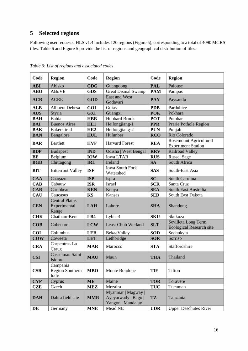
5 Selected regions

Following user requests, HLS v1.4 includes 120 regions (Figure 5), corresponding to a total of 4090 MGRS

tiles. Table 6 and Figure 5 provide the list of regions and geographical distribution of tiles.

Table 6: List of regions and associated codes

Code Region Code Region Code Region

ABI Abisko GDG Guangdong PAL Palouse

ABO ABoVE GDS Great Dismal Swamp PAM Pampas

ACR ACRE GOD East and West

Godavari PAY Paysandu

ALB Albuera Dehesa GOI Goias PDB Pardubice

AUS Styria GXI Guangxi POK Pokhara

BAH Bahia HBB Hubbard Brook POT Potohar

BAI Buenos Aires HE1 Heilongjiang-1 PPR Prarie Pothole Region

BAK Bakersfield HE2 Heilongjiang-2 PUN Punjab

BAN Bangalore HUL Hulunber RCO Rio Colorado

BAR Bartlett HVF Harvard Forest REA Rosemount Agricultural

Experiment Station

BDP Budapest IND Odisha | West Bengal RRV Railroad Valley

BE Belgium IOW Iowa LTAR RUS Russel Sage

BGD Chittagong IRL Ireland SA South Africa

BIT Bitterroot Valley ISF Iowa South Fork

Watershed SAS South-East Asia

CAA Caagazu ISP Ispra SC South Carolina

CAB Cabauw ISR Israel SCR Santa Cruz

CAR Caribbean KEN Kenya SEA South East Australia

CAU Caucasus KS Kansas SED South East Dakota

CEN

Central Plains

Experimental

Range LAH Lahore SHA Shandong

CHK Chatham-Kent LB4 Lybia-4 SKU Skukuza

COB Cobecore LCW Least Chub Wetland SLT Sevilleta Long Term

Ecological Research site

COL Columbus LEB BekaaValley SOD Sodankyla

COW Coweeta LET Lethbridge SOR Sorriso

CRA Carpentras-La

Craux MAR Marocco STA Staffordshire

CSI Casselman Saint-

Isidore MAU Maun THA Thailand

CSR

Campania

Region Southern

Italy MBO Monte Bondone TIF Tifton

CYP Cyprus ME Maine TOR Toravere

CZE Czech MEZ Mezaira TUC Tucuman

DAH Dahra field site MMR

Myanmar | Magway |

Ayeyarwady | Bago |

Yangon | Mandalay TZ Tanzania

DE Germany MNE Mead NE UDR Upper Deschutes River

17

Code Region Code Region Code Region

DEP Delmarva

Peninsula MON Mongu UIE U of Ill. Energy Farm

DON Donana NA North_America UKR Ukraine

EVE Everglades NEA North East Arkansas UMB U of Mich. Biological

Station

FAJ Fajemyr NID Nile Delta VAI Vaira Ranch

FAQ Aquitaine NOR Norunda VMD Mekong

FCE Centre NOS Norway Spruce VRR Red River

FR France NWG Northwest Georgia WNU Gangneung_WNU

FTB Fontainebleau NWI North Wisconsin YAK Yakutsk-Larch

FUJ Fujian NWO North West Ohio YAQ YaquiValley

GBL Gambella OSR Observatoire Spatial

Regional YUM Yuma

Figure 5: Distribution of 4090 MGRS tiles covered in HLS v1.4. Background image is NASA Blue Marble

product

6 Products formats

6.1 Files format

HLS products are stored in the Hierarchical Data Format (HDF)-4 format, with internal compression. Each

HDF file contains metadata including geoferencing information, as well as data sets on spectral band and

QA band. Each HDF file is also accompanied by an ENVI ASCII text header file containing georeferencing

information.

18

6.2 S10

The S10 product contains MSI surface reflectance at full spatial resolution. Table 7 lists all the Scientific

Data Sets (SDS) of the S10 product.

Table 7: list of the SDS of the S10 product (SR = Surface Reflectance, TOA Refl. = Top-of-Atmosphere

Reflectance)

SDS name

MSI

band

number

Units Data

type Scale

Fill

value

Spatial

Resolution Description

B01 1 reflectance int16 0.0001 -1000 60

SR








B8A 8A reflectance int16 0.0001 -1000 10

B09 9 reflectance int16 0.0001 -1000 60 TOA Refl.


B11 11 reflectance int16 0.0001 -1000 20 SR


QA

(Table 10) - none uint8 - 255 10 Quality bits

19

6.3 S30

The product S30 contains MSI surface reflectance at 30 m spatial resolution. Table 8 lists all the SDS of

the S30 product.

Table 8: list of the SDS of the S30 product (SR = Surface Reflectance, NBAR = Nadir BRDF-Adjusted

Reflectance, TOA Refl. = Top of Atmosphere Reflectance)

SDS name

MSI

band

number

Units Data

type Scale

Fill

value

Spatial


B01 1 reflectance int16 0.0001 -1000 30 SR


NBAR B03 3 reflectance int16 0.0001 -1000 30



SR B06 6 reflectance int16 0.0001 -1000 30


B08 8 reflectance int16 0.0001 -1000 30 NBAR

B8A 8A reflectance int16 0.0001 -1000 30

B09 9 reflectance int16 0.0001 -1000 30 TOA Refl.


B11 11 reflectance int16 0.0001 -1000 30 NBAR


QA


20

6.4 L30

The product L30 contains Landsat-8 OLI surface reflectance and TOA TIRS brightness temperature gridded

at 30 m spatial resolution over the MGRS tiling system. Table 9 lists all the SDS of the L30 product.

Table 9: list of the SDS of the L30 product (SR = Surface Reflectance, NBAR = Nadir BRDF-normalized

Reflectance, TOA Refl. = Top of Atmosphere Reflectance, TOA BT = Top of Atmosphere Brightness

temperature)

SDS name

OLI

band

number

Units Data

type Scale

Fill

value

Spatial


band01 1 reflectance int16 0.0001 -1000 30

NBAR







band09 9 reflectance int16 0.0001 -1000 30 TOA Refl.

band10 10 degree °C int16 0.01 -1000 30 TOA BT

band11 11 degree °C int16 0.01 -1000 30

QA


21

6.5 Quality Assessment layer

Quality Assessment (QA) SDS of the 3 products follows the same bit structure described in Table 10.

Table 10: Description of the bits in the one-byte Quality Assessment layer for the 3 products. Bits are listed

from the MSB (bit 7) to the LSB (bit 0)

Bit number QA description Bit combination Description

7-6 Aerosol Quality

00 Climatology

01 Low

10 Average

11 High

5 Water 1 Yes

0 No

4 Snow/ice 1 Yes

0 No

3 Cloud shadow 1 Yes

0 No

2 Adjacent cloud 1 Yes

0 No

1 Cloud 1 Yes

0 No

0 Cirrus 1 Yes

0 No

Note that due to the union of masks from multiple sources, values of bits 0-5 may not be mutually exclusive,

i.e., two bits may both be set to 1 for the same pixel. See Appendix A on how to decode the QA bits with

simple integer arithmetic.

Users are advised to mask out Cirrus, Cloud and Adjacent cloud pixels. Users requiring high quality land

surface reflectance values with the lowest uncertainties should also mask out Aerosol Quality pixels with

High impact, in addition to cloud and adjacent cloud pixels, recognizing that doing so will decrease the

number of observations available for analysis. Users with less strict requirements and intending to provide

additional post-processing steps, such as time-series filtering/fitting or incorporating quality information

into higher-level algorithms, may use surface reflectance values identified as high aerosol and mark them

as lower quality compared to other pixels.

22

6.6 Metadata dictionary

Metadata about the product are encapsulated in the HDF file. Those metadata can be extracted, for example

through GDAL command gdalinfo, or HDF command ncdump -h. The metadata fields are:

ACCODE: LaSRC version, e.g. LaSRCS2AV3.5.5 or LaSRCL8V3.5.5

AngleBand: 0, 1, 2, 3, 4, 5, 6, 7, 8, 9, 10, 11, 12 [for S10/S30]

arop_ave_xshift(meters): Average X-shift in meter computed over the HLS tile [L30/S30]

arop_ave_yshift(meters): Average Y-shift in meter computed over the HLS tile [L30/S30]

arop_ncp: Number of control point found by AROP [L30/S30]

arop_rmse(meters): RMSE of co-registration to the reference image

arop_s2_refimg: S10 product name used as based image for AROP [L30/S30]

cloud_coverage: cloud coverage per tile

DATASTRIP_ID: Datastrip name in the SAFE file [S30/S10]

DATA_TYPE: Landsat 8 Levele-1 product, e.g. L1GT [L30]

HLS_PROCESSING_TIME: HLS Processing date and time [S30/S10/L30]

HORIZONTAL_CS_CODE: Projection code in EPSG format, e.g. EPSG:32618 [S30/S10]

HORIZONTAL_CS_NAME: Projection name, e.g. WGS84 / UTM zone 18N [S30/S10/L30]

L1C_IMAGE_QUALITY: Sentinel-2 L1C product quality control, including the following

quality controls: "SENSOR", "GEOMETRIC", "GENERAL", "FORMAT" and

"RADIOMETRIC", related to the following value: "PASSED" or "FAILED". The "NONE"

metadata value means all quality controls were set to PASSED [S30]

L1_PROCESSING_TIME: Input Level-1 product processing date [S30/S10/L30]

LANDSAT_PRODUCT_ID: Landsat-8 product ID name, e.g.

LC08_L1GT_014033_20170103_20170218_01_T2 [L30]

LANDSAT_SCENE_ID: Landsat-8 scene ID name, e.g. LC80140332017003LGN01 [L30]

MEAN_SUN_AZIMUTH_ANGLE: Mean Sun Azimuth Angle in degree of the input data

[S30/S10/L30]

MEAN_SUN_ZENITH_ANGLE: Mean Sun Zenith Angle in degree of the input data

[S30/S10/L30]

MEAN_VIEW_AZIMUTH_ANGLE: Mean View Azimuth Angle in degree of the input data

[S30/S10]

MEAN_VIEW_ZENITH_ANGLE: Mean View Zenith Angle in degree of the input data

[S30/S10]

NBAR_Solar_Zenith: Mean Sun Zenith Angle in degree of the HLS product after BRDF-

adjustment [S30/L30]

NCOLS: Number of columns [S30/S10/L30]

NROWS: Number of rows [S30/S10/L30]

PROCESSING_BASELINE: processing baseline for Sentinel-2, e.g. 02.04 [S10/S30]

PRODUCT_URI: Tile directory name in the SAFE (Sentinel Standard Archive Format for

Europe) file [S30/S10]

SENSING_TIME: Image sensing date/time, e.g. 2017-01-06T16:00:50.223Z [S30/S10/L30]

SENSOR: Input Sensor [S10/L30]

SPACECRAFT_NAME: remote sensing satellite, e.g. Sentinel-2A [S10/S30]

spatial_coverage: Percentage of HLS tile with data [S30/S10]

23

SPATIAL_RESOLUTION: HLS spatial resolution in meter [S30/S10/L30]

TILE_ID: Sentinel-2 tile identifier, e.g.

S2A_OPER_MSI_L1C_TL_MTI__20170106T205741_A008059_T18SUJ_N02.04 [S10/S30]

TIRS_SSM_MODEL: TIRS SSM encoder position model (Preliminary, Final or Actual) see

http://landsat.gsfc.nasa.gov/?p=12294 [L30]

TIRS_SSM_POSITION_STATUS [L30]

ULX: X-coordinate of the Upper-left corner of the Upper-left pixel [S30/S10/L30]

ULY: Y-coordinate of the Upper-left corner of the Upper-left pixel [S30/S10/L30]

USGS_SOFTWARE = "LPGS_2.6.2" ;

S10/S30 products have also bandpass adjustment coefficients:

MSI band 01 bandpass adjustment slope and offset=0.995900, -0.000200



MSI band 04 bandpass adjustment slope and offset=0.976500, 0.000900



MSI band 8a bandpass adjustment slope and offset=0.998300, -0.000100

6.7 File naming

All the spectral measurements and QA data from a given sensor on a day for a tile are saved in a single

HDF, named with the following naming convention:

HLS.<HLS_Product>.T<Tile_ID>.<year><doy>.v<version_number>.hdf

where:

<HLS_Product> is the HLS product type (S10, S30 or L30) [3 symbols]

<Tile_ID> is the MGRS Tile ID [5 digits]

<Year> is the sensing time year [4 digits]

<Doy> is the sensing time day of year [3 digits]

<Version_number> is the HLS version number (e.g., 1.2, major and minor changes reflected in the

first and second digits respectively) [3 digits]

For example:

HLS.S30.T18SUJ.2017006.v1.4.hdf

HLS.L30.T18SUJ.2017003.v1.4.hdf

6.8 Product access

The S30 and L30 files are available at https://hls.gsfc.nasa.gov/data/. The v1.4 data directory structure is

slightly different from that of v1.3, as follows:

<HLS_Product>/<year>/<Tile_subdir>/

where

http://landsat.gsfc.nasa.gov/?p=12294

24

<HLS_Product> is the HLS product type (S30 or L30) [3 characters]

<Year> is the sensing time year [4 digits]

<Tile_subdir> is sub-directory path for an HLS Tile ID decomposed into 4 parts. For example, tile

11SPC corresponds to a sub-directory 11/S/P/C/; L30 data of 2018 for tile 11SPC are at

https://hls.gsfc.nasa.gov/data/v1.4/L30/2018/11/S/P/C/

A Bash script is made available at the HLS website to help download the products for an environment

where either the Linux command wget or curl is available. See Appendix B for the script usage.

S10 products are available upon request for special test cases.

7 Quality Control

An evaluation of the S30 and L30 products has been pursued. It follows the methodology of the cross-

comparison of surface reflectance with MODIS Climate Modelling Grid (CMG) products (MOD09CMG)

involving BRDF and spectral adjustment (Claverie et al. 2015). The results are gathered into HTML tables

which show overall scores of the cross-comparison for each product, and individual QA graphics are linked

in the table (Figure 6). For each tile and each site (Table 6), html tables and overall scatter plots are provided.

True color Quick-look images are also produced for each L30 and S30 products at 60m spatial resolution

(Figure 7), highlighting the main QA layers: Water, snow, cloud, cirrus, and shadow. Links to the quick-

look images are provided in the HTML tables.

Figure 6: QA of a sample S30 product (HLS.S30.T31TCJ.2018096.v1.4.hdf). Boxplots show, for each

spectral band, the deviation between HLS and MODIS surface reflectance. The median is displayed with

the red circle, the bold line represents the 1st and 3rd quartiles, and the outliers are displayed with black

crosses.

ftp://hls.gsfc.nasa.gov/pub/QA/QuickLookFR/

25

Figure 7: Quick-look of a sample S30 product, using Red, NIR and SWIR 1.6 spectral bands. Water bodies

are delineated with blue lines, snow with yellow, cloud with red, cirrus clouds with magenta, and shadow

with grey. Interiors of listed bodies are dashed.

Looking at the performance of downstream products that could be in turn be compared to independent

“truth”, can provide additional evidence of the performance of the HLS surface reflectance product. The

Landsat and Sentinel 2 class of sensors by themselves could not derive albedo, which by definition

necessitates the integration of several different viewing geometries. However, the albedo can be estimated

using MODIS by the inversion of the BRDF (Schaaf et al., 2002). By combining MODIS BRDF

information and Landsat data and spatially disaggregating the coarse resolution information, one can derive

a reasonable estimate of a HLS spatial scale Broadband Albedo, as shown by several authors by comparison

to flux tower measurements (Franch, B., et al., 2014a, Shuai, Y., et al., 2011). The Franch et al. (2014a)

algorithm derives a Landsat surface albedo based on the BRDF parameters estimated from the

MODIS CMG surface reflectance product (M{O,Y}D09) using the VJB method (Vermote et al., 2009;

26

Franch et al., 2014b). The algorithm uses a Landsat unsupervised classification to disaggregate the BRDF

parameters to the HLS spatial resolution. The method of Franch et al. (2014a) is directly applied to the HLS

product from 2013 to 2017 over five SURFRAD sites (i.e. Desert Rock, Table Mountain, Bondville,

Goodwin Creek and Penn State University). The results are presented in Figure 8 showing separately the

statistics for Landsat (red) and Sentinel 2 (blue). Figure 8 shows a good agreement of both Landsat and

Sentinel 2 products with field measurements with similar correlation coefficients. The Landsat albedo

shows slightly better statistics than the Sentinel 2 albedo with s difference in RMSE of 0.003 (on the order

of 1%) and a slope nearer to one. However, given the statistical significance of the data analyzed and the

lower number of Sentinel 2 data, both sensors show equivalent performance. These errors are equivalent to

the errors showed in Franch et al. (2014a) for Landsat TM and ETM+ and in Vermote et al. (2016) for

Landsat 8.

Figure 8: Validation of the HLS surface albedo using Franch et al. (2014a) method.

8 Known issues

Fmask for Sentinel-2 can generate erroneous results, particularly for hazy conditions, thin clouds,

cloud edges, and bright urban areas. Distinction between snow and cloud pixels can be inaccurate

due to the lack of thermal data.

The LaSRC cloud mask often confuses cloud with bright urban areas. Users are cautioned to

examine other cloud masking options for urban areas.

27

References

Claverie, M., Vermote, E., Franch, B., & Masek, J. (2015). Evaluation of the Landsat-5 TM and Landsat-7

ETM + surface reflectance products. Remote Sensing of Environment, 169, 390-403.

Claverie, M., Ju, J., Masek, J.G., Dungan, J.L., Vermote, E.F., Roger, J.-C., Skakun, S.V., & Justice, C.O.

(2018). The Harmonized Landsat and Sentinel-2 surface reflectance data set, in press, Remote Sensing of

Environment.

Doxani, G., Vermote, E., Roger, J. C., Gascon, F., Adriaensen, S., Frantz, D., ... & Louis, J. (2018).

Atmospheric correction inter-comparison exercise. Remote Sensing, 10(2), 352.

ESA (2018). Sentinel-2 Data Quality Report S2-PDGS-MPC-DQR.

Franch, B., Vermote, E.F., Claverie, M., (2014a). Intercomparison of Landsat albedo retrieval techniques

and evaluation against in situ measurements across the US SURFRAD network. Remote Sensing of

Environment, 152, 627-637.

Franch, B., Vermote, E. F., Sobrino, J. A., & Julien, Y. (2014b). Retrieval of surface albedo on a daily

basis: Application to MODIS data. IEEE Transactions on Geoscience and Remote Sensing, 52(12), 7549-

7558.

Gao, F., Masek, J.G., & Wolfe, R.E. (2009). Automated registration and orthorectification package for

Landsat and Landsat-like data processing. Journal of Applied Remote Sensing, 3(1), 033515.

Masek, J. G., Vermote, E. F., Saleous, N. E., Wolfe, R., Hall, F. G., Huemmrich, K. F., ... & Lim, T. K.

(2006). A Landsat surface reflectance dataset for North America, 1990-2000. IEEE Geoscience and Remote

Sensing Letters, 3(1), 68-72.

Roy, D. P., Li, J., Zhang, H. K., Yan, L., Huang, H., & Li, Z. (2017). Examination of Sentinel-2A multi-

spectral instrument (MSI) reflectance anisotropy and the suitability of a general method to normalize MSI

reflectance to nadir BRDF adjusted reflectance. Remote Sensing of Environment, 199, 25-38.

Roy, D.P., Zhang, H.K., Ju, J., Gomez-Dans, J.L., Lewis, P.E., Schaaf, C.B., Sun, Q., Li, J., Huang, H., &

Kovalskyy, V. (2016). A general method to normalize Landsat reflectance data to nadir BRDF adjusted

reflectance. Remote Sensing of Environment, 176, 255-271.

Schaaf, C. B., Gao, F., Strahler, A. H., Lucht, W., Li, X., Tsang, T., ... & Lewis, P. (2002). First operational

BRDF, albedo nadir reflectance products from MODIS. Remote Sensing of Environment, 83(1-2), 135-148.

Shuai, Y., Masek, J. G., Gao, F., & Schaaf, C. B. (2011). An algorithm for the retrieval of 30-m snow-free

albedo from Landsat surface reflectance and MODIS BRDF. Remote Sensing of Environment, 115(9),

2204-2216.

Skakun, S., Roger, J. C., Vermote, E. F., Masek, J. G., & Justice, C. O. (2017). Automatic sub-pixel co-

registration of Landsat-8 Operational Land Imager and Sentinel-2A Multi-Spectral Instrument images using

phase correlation and machine learning based mapping. International Journal of Digital Earth, 10(12),

1253-1269.

Storey, J., Choate, M., & Lee, K. (2014). Landsat 8 Operational Land Imager On-Orbit Geometric

Calibration and Performance. Remote Sensing, 6, 11127-11152

Storey, J., Roy, D. P., Masek, J., Gascon, F., Dwyer, J., & Choate, M. (2016). A note on the temporary

misregistration of Landsat-8 Operational Land Imager (OLI) and Sentinel-2 Multi Spectral Instrument

(MSI) imagery. Remote Sensing of Environment, 186, 121-122.

Strahler, A.H., Lucht, W., Schaaf, C.B., Tsang, T., Gao, F., Li, X., Lewis, P., & Barnsley, M. (1999).

MODIS BRDF/Albedo Product: Algorithm Theoretical Basis Document Version 5.0. In M. documentation

(Ed.). Boston.

Vermote, E., Justice, C. O., & Bréon, F. M. (2009). Towards a generalized approach for correction of the

BRDF effect in MODIS directional reflectances. IEEE Transactions on Geoscience and Remote

Sensing, 47(3), 898-908.

28

Vermote, E., Justice, C., Claverie, M., & Franch, B. (2016). Preliminary analysis of the performance of the

Landsat 8/OLI land surface reflectance product. Remote Sensing of Environment, 185, 46-56.

Vermote, E. F., & Kotchenova, S. (2008). Atmospheric correction for the monitoring of land

surfaces. Journal of Geophysical Research: Atmospheres, 113(D23).

Yan, L., Roy, D. P., Li, Z., Zhang, H. K., & Huang, H. (2018). Sentinel-2A multi-temporal misregistration

characterization and an orbit-based sub-pixel registration methodology. Remote Sensing of Environment,

215, 495-506.

Zhang, H.K., Roy, D.P., & Kovalskyy, V. (2016). Optimal Solar Geometry Definition for Global Long-

Term Landsat Time-Series Bidirectional Reflectance Normalization. IEEE Transactions on Geoscience

and Remote Sensing, 54, 1410-1418.

Zhu, Z., Wang, S., & Woodcock, C.E. (2015). Improvement and expansion of the Fmask algorithm: cloud,

cloud shadow, and snow detection for Landsats 4-7, 8, and Sentinel 2 images. Remote Sensing of

Environment, 159, 269-277.

29

Acknowledgment

We thank Feng Gao for providing and spending many hours adapting the AROP code for HLS with quick

turnaround. We also thank Jan Dempewolf for offering his Python script which works around the GDAL-

incompatible issue in HLS v1.3 and it has proved very useful for many people. We also thank Shuang Li,

Min Feng, and Mark Broich for GDAL-test HLS v1.4.

Appendix A. How to decode the bit-packed QA

Quality Assessment (QA) encoded at the bit level provides concise presentation but is less convenient for

users new to this format. This appendix shows how to decode the QA bits with simple integer arithmetic

and no explicit bit operation at all. An analogy in the decimal system illustrates the idea. Suppose we want

to get the digit of the hundreds place of an integer 3215. First divide the integer by 10^2 (i.e. 100) to get an

integer quotient 32, then the digit of the ones place (the least significant digit) of the quotient is what we

want. By computing 32 – ((32 / 10) * 10), we get 2, the digit in the hundreds place of 3215. (Note that in

integer arithmetic 32/10 evaluates to 3.) The same idea applies to binary integers. Suppose we get a decimal

QA value 100, which translates into binary 01100100, indicating that the aerosol level is low (bits 6-7), it

is water (bit 5), and adjacent to cloud (bit 2). Suppose we want to find whether it is water, by examining

the value of bit 5. It can be achieved in two steps:

Divide 100 by 2^5 to get the quotient, 3 in this case for integer arithmetic

Find the value of the least significant bit of the quotient by computing 3 – ((3/2) * 2), which is 1

The pixel is water based on the QA byte. Note that Step 2 above is essentially an odd/even number test. All

the bits can be decoded with a loop.

Appendix B. A Bash script to download HLS data

A Bash script available at the HLS home page can be used to download the HLS data in a Bash shell

environment which has either the wget or the curl command. The script can download for a single tile ID,

or multiple tile IDs given in a text file, for all the years or a given year. Download the script and make it

executable. The script works in three ways.

$ ~/bin/download.hls.sh -t 11SPC /tmp/mydata/

This downloads all the years of L30 and S30 data for tile 11SPC into /tmp/mydata/, saved as

/tmp/mydata/11SPC/2013/L30/*hdf

/tmp/mydata/11SPC/2014/L30/*hdf

…

/tmp/mydata/11SPC/2015/S30/*hdf

…

$ ~/bin/download.hls.sh -t 11SPC -y 2017 /tmp/mydata/

This downloads L30 and S30 for year 2017 only.

$ ~/bin/download.hls.sh -t mytiles -y 2017 /tmp/mydata/

30

In this example a text file named mytiles is given to specify multiple 5-character tile IDs delimited by white

space characters (space, tab, or newline). Without the -y option, data of all years will be downloaded for all

the specified tiles.

The script downloads data incrementally. If an earlier downloading process has been interrupted, the

invocation of the same command skips the already downloaded files and continues with the new files. This

also applied to daily routine download (e.g. a cron job).

harmonized landsat sentinel-2 (hls) product user’s guide · 8 3.2 overall hls processing...

Documents