harmonic skeleton for realistic character animation - … · eurographics/ acm siggraph symposium...

Eurographics/ ACM SIGGRAPH Symposium on Computer Animation (2007)D. Metaxas and J. Popovic (Editors)

Harmonic Skeleton for Realistic Character Animation

Grégoire Aujay1 Franck Hétroy1 Francis Lazarus2 Christine Depraz1

1EVASION - LJK (CNRS, INRIA and Univ. Grenoble)2GIPSA-Lab (CNRS and Univ. Grenoble)

AbstractCurrent approaches to skeleton generation are based on topological and geometrical information only; this canbe insufficient for realistic character animation, since the location of the joints does not usually match the realbone structure of the model. This paper proposes the use of anatomical information to enhance the skeleton. Usinga harmonic function, this information can be recovered from the skeleton itself, which is guaranteed not to haveundesired endpoints. The skeleton is computed as a Reeb graph of such a function over the surface of the model.Starting from one point selected on the head of the character, the entire process is fast, automatic and robust; itgenerates skeletons whose joints can be associated with the character’s anatomy. Results are provided, includinga quantitative validation of the generated skeletons.

Categories and Subject Descriptors (according to ACM CCS): I.3.7 [Computer Graphics]: Three-DimensionalGraphics and Realism: Animation

1. Introduction

A common technique for animating a 3D model consists ofcreating a hierarchical articulated structure, named skeleton(or IK skeleton), whose deformation drives the deformationof the associated model. The location and displacement ofthe skeleton’s joints dictate how the model moves (see Fig-ure 1 for an example). A skeleton attached to a 3D model(usually represented as a mesh) can be either created by handor computed. In the case of the realistic animation of a char-acter (be it a human, an animal or a made-up monster), thefirst option is most often chosen by artists, although it isa time-consuming task which needs a skilled user. Indeed,professional artists may create an initial skeleton relativelyquickly, but often need to make many adjustments duringthe rigging process because the skin is very sensitive to theexact location of the skeleton’s joints: they often have to goback and forth several times between skeleton skinning andtesting animation before getting it right. Automatic or semi-automatic methods have several drawbacks: they often allowlittle control over the result, they can produce noisy skele-tons with unwanted joints, and most importantly they relyon the topology and the geometry of the model only, whichis not sufficient for realistic animation where the anatomy ofthe model does not completely match its geometry. For in-stance, in most cases the spine of a character is close to its

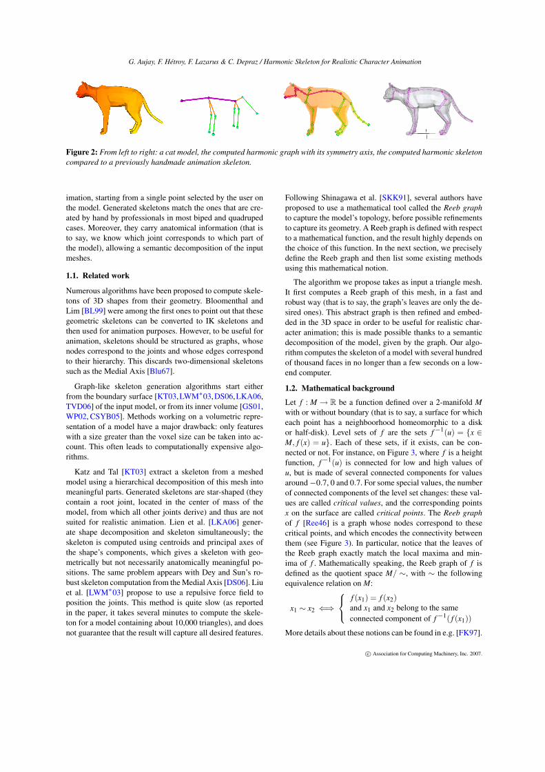
back, while the corresponding axis in computer-generatedskeletons is usually centered within the body (see Figure 12).Moreover, animation skeletons may have some joints whichdo not match any anatomical part of the model but are usefulfor animation purpose (e.g., on the head, see Figure 2).

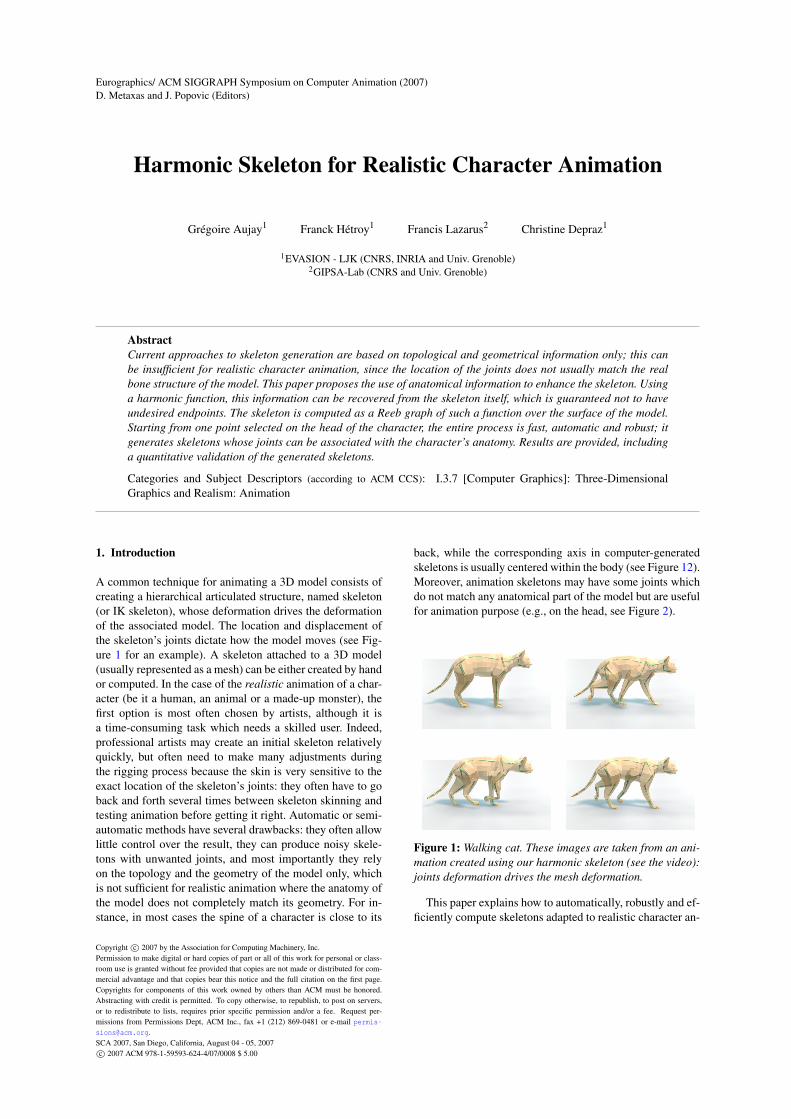
Figure 1: Walking cat. These images are taken from an ani-mation created using our harmonic skeleton (see the video):joints deformation drives the mesh deformation.

This paper explains how to automatically, robustly and ef-ficiently compute skeletons adapted to realistic character an-

Copyright c© 2007 by the Association for Computing Machinery, Inc.Permission to make digital or hard copies of part or all of this work for personal or class-room use is granted without fee provided that copies are not made or distributed for com-mercial advantage and that copies bear this notice and the full citation on the first page.Copyrights for components of this work owned by others than ACM must be honored.Abstracting with credit is permitted. To copy otherwise, to republish, to post on servers,or to redistribute to lists, requires prior specific permission and/or a fee. Request per-missions from Permissions Dept, ACM Inc., fax +1 (212) 869-0481 or e-mail [email protected] 2007, San Diego, California, August 04 - 05, 2007c© 2007 ACM 978-1-59593-624-4/07/0008 $ 5.00

mailto:[email protected]

mailto:[email protected]

G. Aujay, F. Hétroy, F. Lazarus & C. Depraz / Harmonic Skeleton for Realistic Character Animation

Figure 2: From left to right: a cat model, the computed harmonic graph with its symmetry axis, the computed harmonic skeletoncompared to a previously handmade animation skeleton.

imation, starting from a single point selected by the user onthe model. Generated skeletons match the ones that are cre-ated by hand by professionals in most biped and quadrupedcases. Moreover, they carry anatomical information (that isto say, we know which joint corresponds to which part ofthe model), allowing a semantic decomposition of the inputmeshes.

1.1. Related work

Numerous algorithms have been proposed to compute skele-tons of 3D shapes from their geometry. Bloomenthal andLim [BL99] were among the first ones to point out that thesegeometric skeletons can be converted to IK skeletons andthen used for animation purposes. However, to be useful foranimation, skeletons should be structured as graphs, whosenodes correspond to the joints and whose edges correspondto their hierarchy. This discards two-dimensional skeletonssuch as the Medial Axis [Blu67].

Graph-like skeleton generation algorithms start eitherfrom the boundary surface [KT03,LWM∗03,DS06,LKA06,TVD06] of the input model, or from its inner volume [GS01,WP02, CSYB05]. Methods working on a volumetric repre-sentation of a model have a major drawback: only featureswith a size greater than the voxel size can be taken into ac-count. This often leads to computationally expensive algo-rithms.

Katz and Tal [KT03] extract a skeleton from a meshedmodel using a hierarchical decomposition of this mesh intomeaningful parts. Generated skeletons are star-shaped (theycontain a root joint, located in the center of mass of themodel, from which all other joints derive) and thus are notsuited for realistic animation. Lien et al. [LKA06] gener-ate shape decomposition and skeleton simultaneously; theskeleton is computed using centroids and principal axes ofthe shape’s components, which gives a skeleton with geo-metrically but not necessarily anatomically meaningful po-sitions. The same problem appears with Dey and Sun’s ro-bust skeleton computation from the Medial Axis [DS06]. Liuet al. [LWM∗03] propose to use a repulsive force field toposition the joints. This method is quite slow (as reportedin the paper, it takes several minutes to compute the skele-ton for a model containing about 10,000 triangles), and doesnot guarantee that the result will capture all desired features.

Following Shinagawa et al. [SKK91], several authors haveproposed to use a mathematical tool called the Reeb graphto capture the model’s topology, before possible refinementsto capture its geometry. A Reeb graph is defined with respectto a mathematical function, and the result highly depends onthe choice of this function. In the next section, we preciselydefine the Reeb graph and then list some existing methodsusing this mathematical notion.

The algorithm we propose takes as input a triangle mesh.It first computes a Reeb graph of this mesh, in a fast androbust way (that is to say, the graph’s leaves are only the de-sired ones). This abstract graph is then refined and embed-ded in the 3D space in order to be useful for realistic char-acter animation; this is made possible thanks to a semanticdecomposition of the model, given by the graph. Our algo-rithm computes the skeleton of a model with several hundredof thousand faces in no longer than a few seconds on a low-end computer.

1.2. Mathematical background

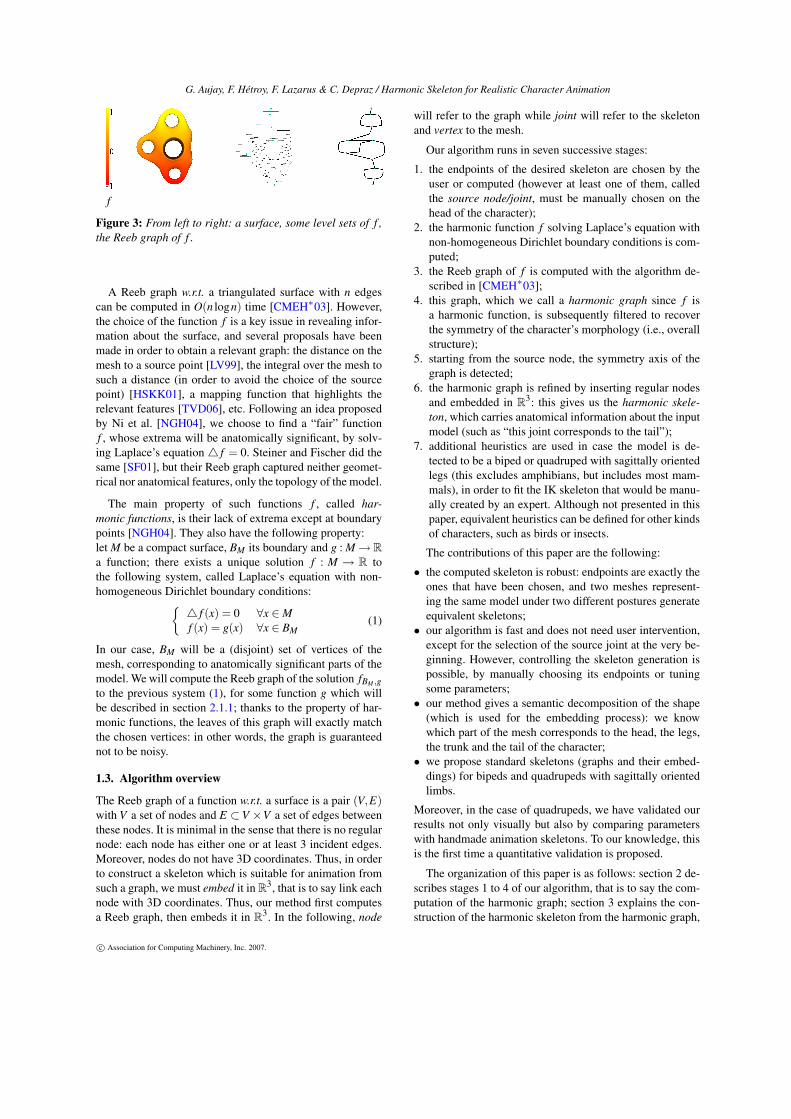
Let f : M → R be a function defined over a 2-manifold Mwith or without boundary (that is to say, a surface for whicheach point has a neighboorhood homeomorphic to a diskor half-disk). Level sets of f are the sets f−1(u) = {x ∈M, f (x) = u}. Each of these sets, if it exists, can be con-nected or not. For instance, on Figure 3, where f is a heightfunction, f−1(u) is connected for low and high values ofu, but is made of several connected components for valuesaround−0.7, 0 and 0.7. For some special values, the numberof connected components of the level set changes: these val-ues are called critical values, and the corresponding pointsx on the surface are called critical points. The Reeb graphof f [Ree46] is a graph whose nodes correspond to thesecritical points, and which encodes the connectivity betweenthem (see Figure 3). In particular, notice that the leaves ofthe Reeb graph exactly match the local maxima and min-ima of f . Mathematically speaking, the Reeb graph of f isdefined as the quotient space M/ ∼, with ∼ the followingequivalence relation on M:

x1 ∼ x2 ⇐⇒

f (x1) = f (x2)and x1 and x2 belong to the sameconnected component of f−1( f (x1))

More details about these notions can be found in e.g. [FK97].

c© Association for Computing Machinery, Inc. 2007.


f

Figure 3: From left to right: a surface, some level sets of f ,the Reeb graph of f .

A Reeb graph w.r.t. a triangulated surface with n edgescan be computed in O(n logn) time [CMEH∗03]. However,the choice of the function f is a key issue in revealing infor-mation about the surface, and several proposals have beenmade in order to obtain a relevant graph: the distance on themesh to a source point [LV99], the integral over the mesh tosuch a distance (in order to avoid the choice of the sourcepoint) [HSKK01], a mapping function that highlights therelevant features [TVD06], etc. Following an idea proposedby Ni et al. [NGH04], we choose to find a “fair” functionf , whose extrema will be anatomically significant, by solv-ing Laplace’s equation 4 f = 0. Steiner and Fischer did thesame [SF01], but their Reeb graph captured neither geomet-rical nor anatomical features, only the topology of the model.

The main property of such functions f , called har-monic functions, is their lack of extrema except at boundarypoints [NGH04]. They also have the following property:let M be a compact surface, BM its boundary and g : M→ Ra function; there exists a unique solution f : M → R tothe following system, called Laplace’s equation with non-homogeneous Dirichlet boundary conditions:{

4 f (x) = 0 ∀x ∈Mf (x) = g(x) ∀x ∈ BM

(1)

In our case, BM will be a (disjoint) set of vertices of themesh, corresponding to anatomically significant parts of themodel. We will compute the Reeb graph of the solution fBM ,gto the previous system (1), for some function g which willbe described in section 2.1.1; thanks to the property of har-monic functions, the leaves of this graph will exactly matchthe chosen vertices: in other words, the graph is guaranteednot to be noisy.

1.3. Algorithm overview

The Reeb graph of a function w.r.t. a surface is a pair (V,E)with V a set of nodes and E ⊂V ×V a set of edges betweenthese nodes. It is minimal in the sense that there is no regularnode: each node has either one or at least 3 incident edges.Moreover, nodes do not have 3D coordinates. Thus, in orderto construct a skeleton which is suitable for animation fromsuch a graph, we must embed it in R3, that is to say link eachnode with 3D coordinates. Thus, our method first computesa Reeb graph, then embeds it in R3. In the following, node

will refer to the graph while joint will refer to the skeletonand vertex to the mesh.

Our algorithm runs in seven successive stages:

1. the endpoints of the desired skeleton are chosen by theuser or computed (however at least one of them, calledthe source node/joint, must be manually chosen on thehead of the character);

2. the harmonic function f solving Laplace’s equation withnon-homogeneous Dirichlet boundary conditions is com-puted;

3. the Reeb graph of f is computed with the algorithm de-scribed in [CMEH∗03];

4. this graph, which we call a harmonic graph since f isa harmonic function, is subsequently filtered to recoverthe symmetry of the character’s morphology (i.e., overallstructure);

5. starting from the source node, the symmetry axis of thegraph is detected;

6. the harmonic graph is refined by inserting regular nodesand embedded in R3: this gives us the harmonic skele-ton, which carries anatomical information about the inputmodel (such as “this joint corresponds to the tail”);

7. additional heuristics are used in case the model is de-tected to be a biped or quadruped with sagittally orientedlegs (this excludes amphibians, but includes most mam-mals), in order to fit the IK skeleton that would be manu-ally created by an expert. Although not presented in thispaper, equivalent heuristics can be defined for other kindsof characters, such as birds or insects.

The contributions of this paper are the following:

• the computed skeleton is robust: endpoints are exactly theones that have been chosen, and two meshes represent-ing the same model under two different postures generateequivalent skeletons;• our algorithm is fast and does not need user intervention,

except for the selection of the source joint at the very be-ginning. However, controlling the skeleton generation ispossible, by manually choosing its endpoints or tuningsome parameters;• our method gives a semantic decomposition of the shape

(which is used for the embedding process): we knowwhich part of the mesh corresponds to the head, the legs,the trunk and the tail of the character;• we propose standard skeletons (graphs and their embed-

dings) for bipeds and quadrupeds with sagittally orientedlimbs.

Moreover, in the case of quadrupeds, we have validated ourresults not only visually but also by comparing parameterswith handmade animation skeletons. To our knowledge, thisis the first time a quantitative validation is proposed.

The organization of this paper is as follows: section 2 de-scribes stages 1 to 4 of our algorithm, that is to say the com-putation of the harmonic graph; section 3 explains the con-struction of the harmonic skeleton from the harmonic graph,



that is to say stages 5 and 6; in section 4, we detail the pro-posed skeletons for bipeds and quadrupeds; we give resultsand discuss them in section 5; finally, we conclude in sec-tion 6.

2. Harmonic graph

2.1. Graph computation

2.1.1. Finding extrema

The first stage of our algorithm is to choose the endpoints ofthe skeleton; they will correspond to extremal joints. Theuser must select one source vertex xsource on the head ofthe character, which will give the source node of the graph.We set f (xsource) = 0. Other endpoints should match rele-vant anatomical features of the character that the user wantsto animate: hands, feet and possibly tail, ears, etc. Theseendpoints can be either selected manually, or computed. Inthe latter case, we try to find vertices x such that the dis-tance d(xsource,x) on the mesh is locally maximum. Severalmethods have been proposed to solve this problem: for in-stance, Dong et al. [DKG05] choose to solve the Poissonequation 4 f = −‖4x‖; the algorithm proposed by Tiernyet al. [TVD06] can also be applied, but it does not use thesource vertex, which should be selected afterwards amongthe detected feature vertices, hence it does not ensure thisvertex will be on the head of the character. The same prob-lem arises when computing the average geodesic distancefunction over the mesh, as did Zhang et al. [ZMT05]. In ourimplementation, we use a fast and more straightforward so-lution: g is defined as a geodesic distance to xsource; we useDijkstra’s algorithm to compute shortest paths on the meshfrom the source vertex to all other vertices, as proposed byLazarus and Verroust [LV99]. This method, as Dong’s, hasone drawback: multiple neighboring local extrema can befound in almost flat regions. We propose a solution to clus-ter these extrema, which will be discussed in section 2.2.For each extremum vertex x (be it manually or automaticallychosen), the value f (x) is set to the length of the shortestpath from the source vertex, as computed by Dijkstra’s al-gorithm (it could also be set to the value given by Dong’smethod when using this algorithm). Doing so, the harmonicfunction f can be seen as a smooth approximated distance tothe source vertex over the mesh.

2.1.2. Solving Laplace’s equation

Once the boundary conditions to Laplace’s equation are set,the system (1) is solved using a classical finite elementsmethod of P1 type (the function f , defined for each vertex, islinearly interpolated inside each triangle). Since the assem-bled matrix is very sparse, computation can be done veryefficiently (e.g. using the SuperLU solver [DEG∗99]).

2.1.3. Generating the graph

The Reeb graph of f is then computed using Cole-McLaughlin’s algorithm [CMEH∗03]. This algorithm re-quires f to be a Morse function: this basically means that two

neighboring critical points should have two different valuesfor f . To ensure this property, we check if all vertices onthe mesh have different values. If several vertices x1, . . . ,xkhave the same value f (x1) = . . . = f (xk), we order them andchange their values slightly.

2.2. Graph filtering

2.2.1. Recovering the shape’s symmetries

Even if the model is symmetric, Cole-McLaughlin’s algo-rithm may generate a non-symmetric graph, because thesource vertex may not be located exactly on the symmetryplane or axis. We propose here a simple way to recover thesesymmetries.

Each node n of the graph G is assigned with the valuef (x), where x is the critical vertex on the surface correspond-ing to n. Now, let us give weights to the edges of G. Let(n1,n2) be an edge of G. (n1,n2) is balanced by the follow-ing weight:

w(n1,n2) =| f (n1)− f (n2)|

|maxn∈G

f (n)−minn∈G

f (n)| (2)

Considering f as an approximated distance to the source ver-tex over the mesh (see section 2.1.1), w(n1,n2) representsthe normalized difference between the distance to the sourcevertex of two “topologically close” vertices. If w(n1,n2) issmall, this means that the corresponding vertices x1 and x2are approximately at the same distance to the source vertex,and are also located in the same topological area (they arenot necessarily geometrically close to each other). Thus, inorder to recover the shape’s symmetries, we propose to filterthe graph by collapsing every internal edge with a weightlower than a given threshold t1. We do not collapse edgescontaining a leaf node, since this could remove small fea-tures.

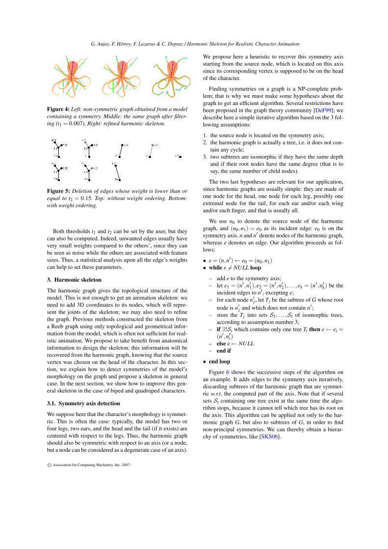
Notice that we can recover not only geometrical symme-tries of the model, but also morphological ones: for instance,the octopus model of Figure 4 is not symmetric, geometri-cally speaking, because its tentacles are not in the same po-sition; it can however be regarded as morphologically sym-metric, because these tentacles have the same size and areregularly placed around a symmetry axis. As shown on thesame model, we can recover not only symmetries w.r.t. aplane but also symmetries w.r.t. an axis.

2.2.2. Removing irrelevant extrema

As explained in section 2.1.1, it may happen that too manyextremum vertices are computed. In order to remove irrel-evant extrema, since extrema correspond exactly to the leafnodes of the graph, we propose to remove the external edges(that is to say edges containing a leaf node) with a weightlower than a given threshold t2, together with their nodes.However, these edges should be removed carefully (see Fig-ure 5): in order to avoid extra deletion of edges, they shouldfirst be ordered by increasing weight.



Figure 4: Left: non-symmetric graph obtained from a modelcontaining a symmetry. Middle: the same graph after filter-ing (t1 = 0.007). Right: refined harmonic skeleton.

Figure 5: Deletion of edges whose weight is lower than orequal to t2 = 0.15. Top: without weight ordering. Bottom:with weight ordering.

Both thresholds t1 and t2 can be set by the user, but theycan also be computed. Indeed, unwanted edges usually havevery small weights compared to the others’, since they canbe seen as noise while the others are associated with featuresizes. Thus, a statistical analysis upon all the edge’s weightscan help to set these parameters.

3. Harmonic skeleton

The harmonic graph gives the topological structure of themodel. This is not enough to get an animation skeleton: weneed to add 3D coordinates to its nodes, which will repre-sent the joints of the skeleton; we may also need to refinethe graph. Previous methods constructed the skeleton froma Reeb graph using only topological and geometrical infor-mation from the model, which is often not sufficient for real-istic animation. We propose to take benefit from anatomicalinformation to design the skeleton; this information will berecovered from the harmonic graph, knowing that the sourcevertex was chosen on the head of the character. In this sec-tion, we explain how to detect symmetries of the model’smorphology on the graph and propose a skeleton in generalcase. In the next section, we show how to improve this gen-eral skeleton in the case of biped and quadruped characters.

3.1. Symmetry axis detection

We suppose here that the character’s morphology is symmet-ric. This is often the case: typically, the model has two orfour legs, two ears, and the head and the tail (if it exists) arecentered with respect to the legs. Thus, the harmonic graphshould also be symmetric with respect to an axis (or a node,but a node can be considered as a degenerate case of an axis).

We propose here a heuristic to recover this symmetry axisstarting from the source node, which is located on this axissince its corresponding vertex is supposed to be on the headof the character.

Finding symmetries on a graph is a NP-complete prob-lem; that is why we must make some hypotheses about thegraph to get an efficient algorithm. Several restrictions havebeen proposed in the graph theory community [DeF99]; wedescribe here a simple iterative algorithm based on the 3 fol-lowing assumptions:

1. the source node is located on the symmetry axis;2. the harmonic graph is actually a tree, i.e. it does not con-

tain any cycle;3. two subtrees are isomorphic if they have the same depth

and if their root nodes have the same degree (that is tosay, the same number of child nodes).

The two last hypotheses are relevant for our application,since harmonic graphs are usually simple: they are made ofone node for the head, one node for each leg, possibly oneextremal node for the tail, for each ear and/or each wingand/or each finger, and that is usually all.

We use n0 to denote the source node of the harmonicgraph, and (n0,n1) = e0 as its incident edge: e0 is on thesymmetry axis. n and n′ denote nodes of the harmonic graph,whereas e denotes an edge. Our algorithm proceeds as fol-lows:

• e = (n,n′)← e0 = (n0,n1)• while e 6= NULL loop

– add e to the symmetry axis;– let e1 = (n′,n′1),e2 = (n′,n′2), . . . ,ek = (n′,n′k) be the

incident edges to n′, excepting e;– for each node n′j, let Tj be the subtree of G whose root

node is n′j and which does not contain n′;– store the Tj into sets S1, . . . ,Sl of isomorphic trees,

according to assumption number 3;– if ∃!Si which contains only one tree Ti then e← ei =

(n′,n′i)– else e← NULL– end if

• end loop

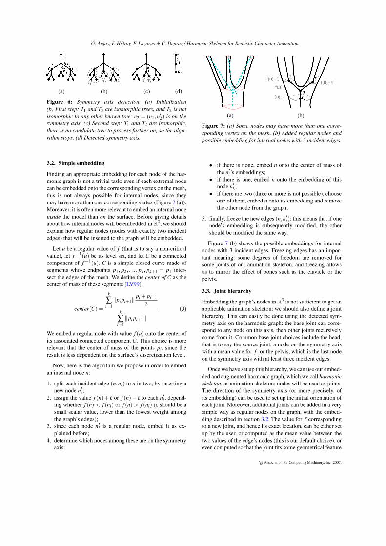
Figure 6 shows the successive steps of the algorithm onan example. It adds edges to the symmetry axis iteratively,discarding subtrees of the harmonic graph that are symmet-ric w.r.t. the computed part of the axis. Note that if severalsets Si containing one tree exist at the same time the algo-rithm stops, because it cannot tell which tree has its root onthe axis. This algorithm can be applied not only to the har-monic graph G, but also to subtrees of G, in order to findnon-principal symmetries. We can thereby obtain a hierar-chy of symmetries, like [SKS06].



(a) (b) (c) (d)

Figure 6: Symmetry axis detection. (a) Initialization(b) First step: T1 and T3 are isomorphic trees, and T2 is notisomorphic to any other known tree: e2 = (n1,n

′2) is on the

symmetry axis. (c) Second step: T1 and T2 are isomorphic,there is no candidate tree to process further on, so the algo-rithm stops. (d) Detected symmetry axis.

3.2. Simple embedding

Finding an appropriate embedding for each node of the har-monic graph is not a trivial task: even if each extremal nodecan be embedded onto the corresponding vertex on the mesh,this is not always possible for internal nodes, since theymay have more than one corresponding vertex (Figure 7 (a)).Moreover, it is often more relevant to embed an internal nodeinside the model than on the surface. Before giving detailsabout how internal nodes will be embedded in R3, we shouldexplain how regular nodes (nodes with exactly two incidentedges) that will be inserted to the graph will be embedded.

Let u be a regular value of f (that is to say a non-criticalvalue), let f−1(u) be its level set, and let C be a connectedcomponent of f−1(u). C is a simple closed curve made ofsegments whose endpoints p1, p2, . . . , pk, pk+1 = p1 inter-sect the edges of the mesh. We define the center of C as thecenter of mass of these segments [LV99]:

center(C) =

k

∑i=1‖pi pi+1‖

pi + pi+12

k

∑i=1‖pi pi+1‖

(3)

We embed a regular node with value f (u) onto the center ofits associated connected component C. This choice is morerelevant that the center of mass of the points pi, since theresult is less dependent on the surface’s discretization level.

Now, here is the algorithm we propose in order to embedan internal node n:

1. split each incident edge (n,ni) to n in two, by inserting anew node n′i ;

2. assign the value f (n)+ ε or f (n)− ε to each n′i , depend-ing whether f (n) < f (ni) or f (n) > f (ni) (ε should be asmall scalar value, lower than the lowest weight amongthe graph’s edges);

3. since each node n′i is a regular node, embed it as ex-plained before;

4. determine which nodes among these are on the symmetryaxis:

(a) (b)

Figure 7: (a) Some nodes may have more than one corre-sponding vertex on the mesh. (b) Added regular nodes andpossible embedding for internal nodes with 3 incident edges.

• if there is none, embed n onto the center of mass ofthe n′i’s embeddings;

• if there is one, embed n onto the embedding of thisnode n′k;

• if there are two (three or more is not possible), chooseone of them, embed n onto its embedding and removethe other node from the graph;

5. finally, freeze the new edges (n,n′i): this means that if onenode’s embedding is subsequently modified, the othershould be modified the same way.

Figure 7 (b) shows the possible embeddings for internalnodes with 3 incident edges. Freezing edges has an impor-tant meaning: some degrees of freedom are removed forsome joints of our animation skeleton, and freezing allowsus to mirror the effect of bones such as the clavicle or thepelvis.

3.3. Joint hierarchy

Embedding the graph’s nodes in R3 is not sufficient to get anapplicable animation skeleton: we should also define a jointhierarchy. This can easily be done using the detected sym-metry axis on the harmonic graph: the base joint can corre-spond to any node on this axis, then other joints recursivelycome from it. Common base joint choices include the head,that is to say the source joint, a node on the symmetry axiswith a mean value for f , or the pelvis, which is the last nodeon the symmetry axis with at least three incident edges.

Once we have set up this hierarchy, we can use our embed-ded and augmented harmonic graph, which we call harmonicskeleton, as animation skeleton: nodes will be used as joints.The direction of the symmetry axis (or more precisely, ofits embedding) can be used to set up the initial orientation ofeach joint. Moreover, additional joints can be added in a verysimple way as regular nodes on the graph, with the embed-ding described in section 3.2. The value for f correspondingto a new joint, and hence its exact location, can be either setup by the user, or computed as the mean value between thetwo values of the edge’s nodes (this is our default choice), oreven computed so that the joint fits some geometrical feature



(e.g. local minimum of the gaussian curvature, as proposedby [TVD06]).

4. Adapted embedding for bipeds and quadrupeds

In this section, we explain how the previously computedskeleton can be modified in order to better fit biped orquadruped mammals. Equivalent heuristics can be devel-oped for other kinds of characters. These heuristics rely onsemantic information about the model’s anatomy associatedto each joint of the skeleton, which can be recovered sincethe source joint corresponds to the head of the character andall skeleton extrema are known (see Figure 8 (a)). First, wepropose a heuristic to check if the skeleton corresponds to abiped or a quadruped model.

4.1. Biped/quadruped discrimination

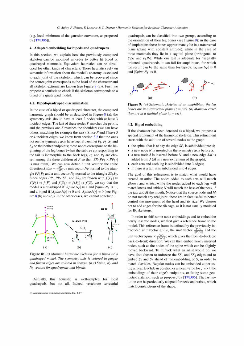
In the case of a biped or quadruped character, the computedharmonic graph should be as described in Figure 8 (a): thesymmetry axis should have at least 2 nodes with at least 3incident edges. The last of these nodes P matches the pelvis,and the previous one S matches the shoulders (we can haveothers, matching for example the ears). Since P and S have 3or 4 incident edges, we know from section 3.2 that the onesnot on the symmetry axis have been frozen: let P1, P2, S1 andS2 be their other endpoints; these nodes correspond to the be-ginning of the leg bones (when the subtree corresponding tothe tail is isomorphic to the back legs, P1 and P2 are cho-sen among the three children of P so that |SP.(PP1×PP2)|is maximum). We can now define 3 unit vectors: the spinedirection Spine = SP

‖SP‖ , a unit vector NP normal to the trian-gle PP1P2 and a unit vector NS normal to the triangle SS1S2.Since edges PP1,PP2,SS1 and SS2 are frozen with f (P1) ≈f (P2) ≈ f (P) and f (S1) ≈ f (S2) ≈ f (S), we say that themodel is a quadruped if |Spine.NP| ≈ 1 and |Spine.NS| ≈ 1,and a biped if |Spine.NP| ≈ 0 and |Spine.NS| ≈ 0 (see Fig-ure 8 (b) and (c)). In the other cases, we cannot conclude.

(a) (b) (c)

Figure 8: (a) Minimal harmonic skeleton for a biped or aquadruped model. The symmetry axis is colored in purpleand frozen edges are colored in orange. (b,c) Spine, NP andNS vectors for quadrupeds and bipeds.

Actually, this heuristic is well-adapted for mostquadrupeds, but not all. Indeed, vertebrate terrestrial

quadrupeds can be classified into two groups, according tothe orientation of their leg bones (see Figure 9): in the caseof amphibians these bones approximately lie in a transversalplane (plane with constant altitude), while in the case ofmost mammals they lie in a sagittal plane (orthogonal toS1S2 and P1P2). While our test is adequate for “sagitallyoriented” quadrupeds, it can fail for amphibians, for whichthe result can be the same than for bipeds: |Spine.NP| ≈ 0and |Spine.NS| ≈ 0.

(a) (b)

Figure 9: (a) Schematic skeleton of an amphibian: the legbones are in a tranversal plane (z = cst). (b) Mammal case:they are in a sagittal plane (x = cst).

4.2. Biped embedding

If the character has been detected as a biped, we propose aspecial refinement of the harmonic skeleton. This refinementstarts with the addition of several nodes to the graph:

• the spine, that is to say the edge SP, is subdivided into 4;• a new node N is inserted on the symmetry axis before S;• a new node J is inserted before N, and a new edge JM is

added from J (M is a new extremum of the graph);• each arm and each leg is subdivided into 3 edges;• if there is a tail, it is subdivided into 4 edges.

The goal of this refinement is to match what would havecreated an artist. The nodes added to each arm will matchelbows and wrists, while the nodes added to each leg willmatch knees and ankles; N will match the base of the neck, Jthe jaw and M the mouth. Notice that the source node and Mdo not match any real joint: these are in fact useful to bettercontrol the movement of the head and its size. We choosenot to add edges for the rib cage, as it is not usually modeledfor IK skeletons.

In order to shift some node embeddings and to embed thenewly inserted nodes, we first give a reference frame to themodel. This reference frame is defined by the previously in-troduced unit vector Spine, the unit vector P1P2

‖P1P2‖ and the

unit vector Spine× P1P2‖P1P2‖ , which gives the front-to-back (or

back-to-front) direction. We can then embed newly insertednodes, such as the nodes of the spine which can be slightlymoved backward. To mimick what an artist would do, wehave also chosen to unfreeze the SS1 and SS2 edges,and toembed S1 and S2 ahead of the embedding of S, in order tomatch clavicles. Regular nodes can be embedded either us-ing a mean Euclidean position or a mean value for f w.r.t. theembeddings of their edge’s endpoints, or fitting some geo-metric criterion, such as proposed by [TVD06]. The last so-lution can be particularly adapted for neck and wrists, whichmatch constrictions of the shape.



4.3. Quadruped embedding

Automatic animation skeleton generation is much less de-veloped for four-footed animals than for bipeds. In orderto refine the harmonic skeleton for parasagittally orientedquadrupeds, we based our work on the reference animationskeletons proposed by [RFDC05]. These IK skeletons wereconstructed by hand, from anatomical references [Cal75].We add the same nodes to the harmonic graph as for bipeds,except that each front leg is subdivided into 5 edges, eachback leg into 4 edges, and instead of having 2 edges betweenJ and S (JN and NS), we have 5: the 4 added nodes willmatch the first, the second, the fourth and the seventh (whichis the last) cervical vertebrae. We also subdivide the edgestarting from the source node in 3; the first inserted node J′

will match the jaw, while this time J will match the cranium.As for bipeds, M does not match any real joint and is usefulto control the head’s size and its movement. It will be put ontop of the head of the character. We use the same referenceframe as for biped embedding; here is how some of the jointsare embedded: P is lifted up along the Spine× P1P2

‖P1P2‖ direc-tion from the simple embedding position (the center of itsconnected component for f−1( f (P))) in order to be close tothe back; nodes on SP are also lifted up, and so are S1, S2, P1and P2; S is lifted up in order to match the pelvis’ height; thefirst inserted nodes on each leg are moved along the −Spinedirection. We found that the best choice to embed the nodeJ was near the neck constriction (actually a bit closer to thesource joint); its value for f and exact location depends onthe neck length. Finally, a simple solution for J′ is along the−Spine× P1P2

‖P1P2‖ direction from J, close to the chin.

5. Results and validation

Figures 2 and 10 to 12 show harmonic skeletons computedwith our method. In these cases extrema have been selectedby hand, because automatic computation of the extremal fea-tures can be quite slow. Thus, the threshold t2 has not beenused (it has been set to zero). No fine tuning of t1 has beennecessary: for almost all models, setting t1 between 0.001and 0.150 is sufficient. Except the selection of the extremaand t1, the entire process is automatic; no post-processinghas been applied.

5.1. Biped and quadruped embeddings

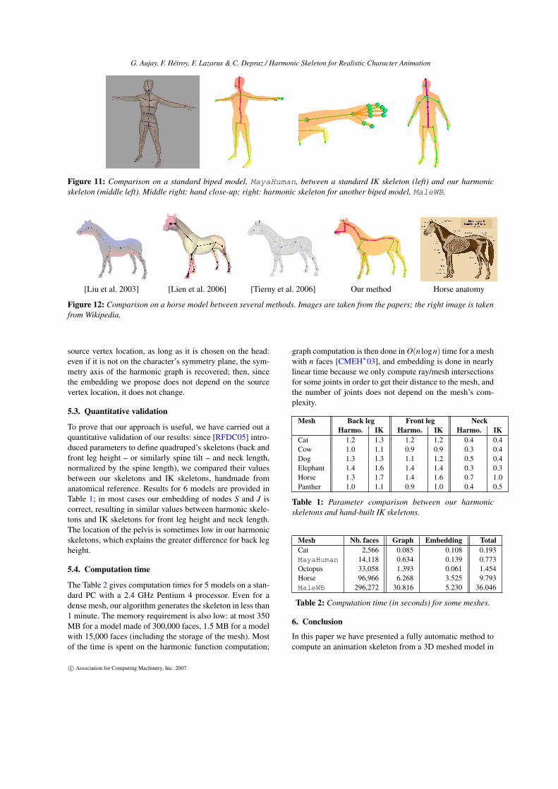
Figure 11 shows the harmonic skeleton computed from abiped model, compared with a standard handmade skeleton(from Autodesk’s Maya software). We have not modeled therib cage, as explained before. As for the other models, thesymmetry axis is colored in purple and frozen edges are col-ored in orange. Even though the graph is more complex thanthe minimal harmonic graph for a biped (Figure 8 (a)) be-cause we decided to model the fingers, the symmetry axishas been correctly detected. Another biped skeleton is shownon the right of the figure. We have chosen to embed extremalnodes onto corresponding vertices on the mesh, but we couldhave easily embedded them inside the model instead, using

a close but regular value for f and the definition (3) of thecenter of a connected component.

Results on two quadruped models are shown on figures 2and 12. The cat’s tail is not considered as part of the sym-metry axis, since its corresponding subtree on the harmonicgraph is isomorphic to the back legs. Our algorithm providesanimation skeletons close to the model’s anatomy and to tra-ditional IK skeletons. Nevertheless, some joints may need tobe slightly displaced for better animation, particularly in thehead. It is also noticeable that the very beginning of the tailis actually included in a frozen edge; this is correct since itcorresponds to the first coccygeal vertebrae which are indeedattached to the sacrum [Cal75].

Our harmonic skeletons have been used for animation, ascan be seen on Figure 1 and on the accompanying video.

5.2. Robustness

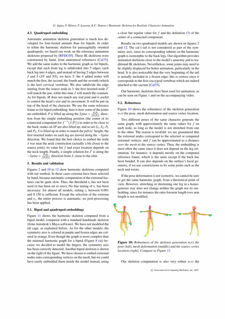
Figure 10 shows the robustness of the skeleton generationw.r.t the pose, mesh deformation and source vertex location.

Two different poses of the same character generate thesame graph, with approximately the same values for f oneach node, as long as the model is not stretched from oneto the other. The reason is twofold: we are guaranteed thatthe extremal nodes correspond to the selected or computedextremal vertices, and f can be approximated as a distanceover the mesh to the source vertex. Then, the embedding ismost often the same since it does not depend on the leg ori-entation, for instance: it depends mostly on the computedreference frame, which is the same except if the back hasbeen bended. It can also depends on the surface’s local ge-ometry, if we use constrictions to fix some joints such as theneck and wrists.

If the pose deformation is not isometric, we cannot be sureto get the same harmonic graph, from a theoretical point ofview. However, stretching or shortening one leg in a homo-geneous way does not change neither the graph nor its em-bedding, since for instance the ratio forearm length over armlength is not modified.

Figure 10: Robustness of the skeleton generation w.r.t thepose (left), mesh deformation (middle) and the source vertexlocation (right). Compare to Figure 11.

Our skeleton computation is also very robust w.r.t the



Figure 11: Comparison on a standard biped model, MayaHuman, between a standard IK skeleton (left) and our harmonicskeleton (middle left). Middle right: hand close-up; right: harmonic skeleton for another biped model, MaleWB.

[Liu et al. 2003] [Lien et al. 2006] [Tierny et al. 2006] Our method Horse anatomy

Figure 12: Comparison on a horse model between several methods. Images are taken from the papers; the right image is takenfrom Wikipedia.

source vertex location, as long as it is chosen on the head:even if it is not on the character’s symmetry plane, the sym-metry axis of the harmonic graph is recovered; then, sincethe embedding we propose does not depend on the sourcevertex location, it does not change.

5.3. Quantitative validation

To prove that our approach is useful, we have carried out aquantitative validation of our results: since [RFDC05] intro-duced parameters to define quadruped’s skeletons (back andfront leg height – or similarly spine tilt – and neck length,normalized by the spine length), we compared their valuesbetween our skeletons and IK skeletons, handmade fromanatomical reference. Results for 6 models are provided inTable 1; in most cases our embedding of nodes S and J iscorrect, resulting in similar values between harmonic skele-tons and IK skeletons for front leg height and neck length.The location of the pelvis is sometimes low in our harmonicskeletons, which explains the greater difference for back legheight.

5.4. Computation time

The Table 2 gives computation times for 5 models on a stan-dard PC with a 2.4 GHz Pentium 4 processor. Even for adense mesh, our algorithm generates the skeleton in less than1 minute. The memory requirement is also low: at most 350MB for a model made of 300,000 faces, 1.5 MB for a modelwith 15,000 faces (including the storage of the mesh). Mostof the time is spent on the harmonic function computation;

graph computation is then done in O(n logn) time for a meshwith n faces [CMEH∗03], and embedding is done in nearlylinear time because we only compute ray/mesh intersectionsfor some joints in order to get their distance to the mesh, andthe number of joints does not depend on the mesh’s com-plexity.

Mesh Back leg Front leg NeckHarmo. IK Harmo. IK Harmo. IK

Cat 1.2 1.3 1.2 1.2 0.4 0.4Cow 1.0 1.1 0.9 0.9 0.3 0.4Dog 1.3 1.3 1.1 1.2 0.5 0.4Elephant 1.4 1.6 1.4 1.4 0.3 0.3Horse 1.3 1.7 1.4 1.6 0.7 1.0Panther 1.0 1.1 0.9 1.0 0.4 0.5

Table 1: Parameter comparison between our harmonicskeletons and hand-built IK skeletons.

Mesh Nb. faces Graph Embedding TotalCat 2,566 0.085 0.108 0.193MayaHuman 14,118 0.634 0.139 0.773Octopus 33,058 1.393 0.061 1.454Horse 96,966 6.268 3.525 9.793MaleWB 296,272 30.816 5.230 36.046

Table 2: Computation time (in seconds) for some meshes.

6. Conclusion

In this paper we have presented a fully automatic method tocompute an animation skeleton from a 3D meshed model in



a few seconds after the selection of an initial point. In thecase of most bipeds or quadrupeds, this skeleton fits the ani-mation skeleton that would be hand-built by an expert start-ing from anatomical boards, and is thus adapted for realisticanimation. The main idea is to construct the Reeb graph ofa harmonic function, which gives the overall morphologicalstructure of the model (especially its symmetry axis), then torefine and embed it using anatomical information. There aretwo main restrictions on the input mesh: it should be a trian-gulated 2-manifold (with or without boundary), and, in orderto recover the symmetry axis of the shape’s morphology, itshould not have handles (otherwise the Reeb graph containscycles). Although the method is fully automatic, the user cancontrol the skeleton generation by tuning a few optional pa-rameters. This tool has been designed both to help artists andto allow non-experts to quickly generate skeletons which canbe used for realistic character animation. Computed skele-tons can be edited and refined, for instance to add joints thatcorrespond to wings or to the trunk of an elephant.

Given this skeleton generation process, we see threepromising research directions. First, each vertex of the meshis related to the joints of the skeleton, since we have givenvalues for the harmonic function to the graph’s nodes, andhence the skeleton’s joints; these relations may be used toenhance skinning weights. Second, our semantic decompo-sition of the graph may also be used to define heuristics thatgive adapted skinning weights: weights may vary accordingto the meaning of neighboring joints. It may also help forautomatic mesh segmentation into anatomically meaningfulregions. Finally, even if not embedded to match the model’sanatomy, the harmonic graph may be useful for other appli-cations (e.g. shape matching), since its construction is robustand does not create unnecessary nodes.

Acknowledgments

The authors would like to thank Lionel Revéret for interest-ing discussions at the beginning of this work. The horse andMaleWB models are courtesy of Cyberware. The MayaHu-man model is courtesy of Autodesk.

References

[BL99] BLOOMENTHAL J., LIM C.: Skeletal methods of shapemanipulation. In Shape Modeling International (1999).

[Blu67] BLUM H.: A transformation for extracting new descrip-tors of shape. In Symposium on Models for the Perception ofSpeech and Visual Form (1967), pp. 362–380.

[Cal75] CALDERON W.: Animal Painting and Anatomy. Dover,1975.

[CMEH∗03] COLE-MCLAUGHLIN K., EDELSBRUNNER H.,HARER J., NATARAJAN V., PASCUCCI V.: Loops in reeb graphsof 2-manifolds. In Symposium on Computational Geometry(2003), pp. 344–350.

[CSYB05] CORNEA N., SILVER D., YUAN X., BALASUBRA-MANIAN R.: Computing hierarchical curve-skeletons of 3d ob-jects. The Visual Computer 21, 11 (2005), 945–955.

[DeF99] DEFRAYSSEIX H.: An heuristic for graph symmetry de-tection. In Symposium on Graph Drawing (1999), pp. 276–285.

[DEG∗99] DEMMEL J., EISENSTAT S., GILBERT J., LI X., LIU

J.: A supernodal approach to sparse partial pivoting. SIAM Jour-nal on Matrix Analysis and Applications 20, 3 (1999), 720–755.

[DKG05] DONG S., KIRCHNER S., GARLAND M.: Harmonicfunctions for quadrilateral remeshing of arbitrary manifolds.Computer Aided Geometric Design, Special issue on GeometryProcessing 22, 5 (2005), 392–423.

[DS06] DEY T., SUN J.: Defining and computing curve-skeletonswith medial geodesic function. In Symposium on Geometry Pro-cessing (2006), pp. 143–152.

[FK97] FOMENKO A., KUNII T.: Topological Modeling for Vi-sualization. Springer-Verlag, 1997.

[GS01] GAGVANI N., SILVER D.: Animating volumetric models.Graphical Models 63, 6 (2001), 443–458.

[HSKK01] HILAGA M., SHINAGAWA Y., KOMURA T., KUNII

T.: Topology matching for fully automatic similarity estimationof 3d shapes. In SIGGRAPH (2001), pp. 203–212.

[KT03] KATZ S., TAL A.: Hierarchical mesh decomposition us-ing fuzzy clustering and cuts. In SIGGRAPH (2003).

[LKA06] LIEN J., KEYSER J., , AMATO N.: Simultaneous shapedecomposition and skeletonization. In ACM Symposium on Solidand Physical Modeling (2006), pp. 219–228.

[LV99] LAZARUS F., VERROUST A.: Level set diagrams of poly-hedral objects. In ACM Symposium on Solid Modeling (1999).

[LWM∗03] LIU P., WU F., MA W., LIANG R., OUHYOUNG M.:Automatic animation skeleton construction using repulsive forcefield. In Pacific Graphics (2003), pp. 409–413.

[NGH04] NI X., GARLAND M., HART J.: Fair morse functionsfor extracting the topological structure of a surface mesh. In SIG-GRAPH (2004), pp. 613–622.

[Ree46] REEB G.: Sur les points singuliers d’une forme de pfaffcomplètement intégrable ou d’une fonction numérique. Comptes-Rendus de l’Académie des Sciences 222 (1946), 847–849.

[RFDC05] REVÉRET L., FAVREAU L., DEPRAZ C., CANI M.:Morphable model of quadruped skeletons for animating 3d ani-mals. In Symposium on Computer Animation (2005).

[SF01] STEINER D., FISCHER A.: Topology recognition of 3dclosed freeform objects based on topological graphs. In PacificGraphics (2001), pp. 82–88.

[SKK91] SHINAGAWA Y., KUNII T., KERGOSIEN Y.: Surfacecoding based on morse theory. IEEE Computer Graphics andApplications 11, 5 (1991), 66–78.

[SKS06] SIMARI P., KALOGERAKIS E., SINGH K.: Foldingmeshes: Hierarchical mesh segmentation based on planar sym-metry. In Symposium on Geometry Processing (2006).

[TVD06] TIERNY J., VANDEBORRE J., DAOUDI M.: 3d meshskeleton extraction using topological and geometrical analyses.In Pacific Graphics (2006), pp. 409–413.

[WP02] WADE L., PARENT R.: Automated generation of controlskeletons for use in animation. The Visual Computer 18 (2002).

[ZMT05] ZHANG E., MISCHAIKOW K., TURK G.: Feature-based surface parameterization and texture mapping. ACMTransactions on Graphics 24, 1 (2005), 1–27.


harmonic skeleton for realistic character animation - … · eurographics/ acm siggraph symposium...

Documents