hardware specialization in deep learning · winograd fp32 fft-1(fft ... hardware-software interface...
TRANSCRIPT

Hardware Specialization in Deep Learning
CSE590W 18Sp, Thursday April 19th 2018Thierry Moreau

Deep Learning Explosion
!2

Deep Learning Revolutionizing Computer Vision
Source: NVIDIA blogpost, June 2016
human ability
!3

Compute Requirements is Steadily Growing
Source: Eugenio Culurciello, An Analysis of Deep Neural Network Models for Practical Applications, arXiv:1605.07678
parameter size
!4
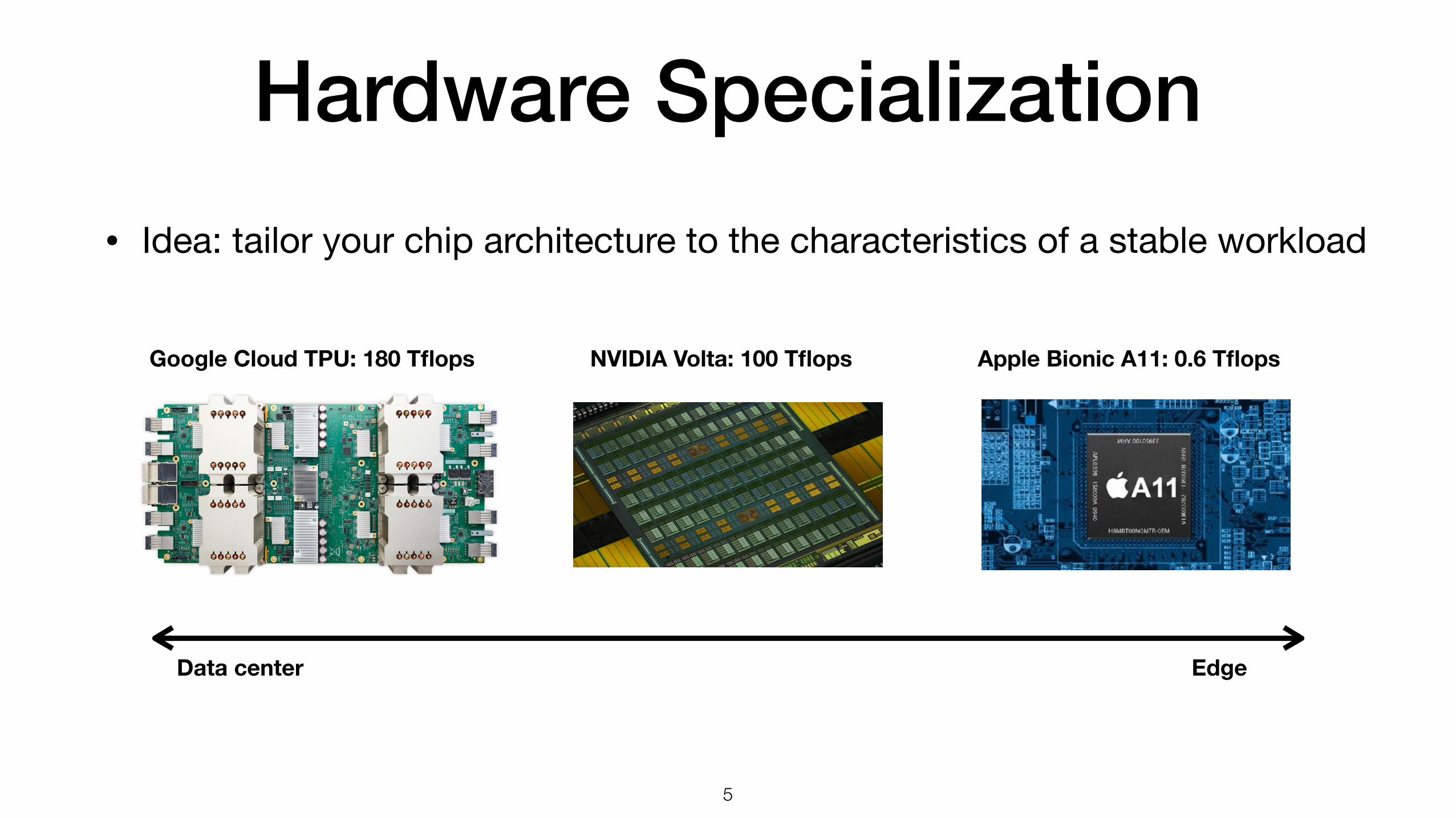
Hardware Specialization• Idea: tailor your chip architecture to the characteristics of a stable workload
Google Cloud TPU: 180 Tflops NVIDIA Volta: 100 Tflops Apple Bionic A11: 0.6 Tflops
Data center Edge
!5

Hardware Specialization• Idea: tailor your chip architecture to the characteristics of a stable workload
Google Cloud TPU: 180 Tflops NVIDIA Volta: 100 Tflops Apple Bionic A11: 0.6 Tflops
Data center Edge
!6

Evolution of Deep LearningMatrix Multiplication: fp32 (A, B) × (B, C)
Optimization New problem specification Reference
quantization int4 (A, B) × bool (B, C) Binary Connect, NIPS 15
knowledge distillation
fp32 (a, b) × (b, c) Fitnets, ICLR 2015
compression, pruning
sparse int16 (A, B) × (B, C) Deep Compression, ICLR 2016
tensor decomposition
fp32 (A,r) x (r,B) × (B,C) Compression of deep convolutional neural networks, ICLR 2016
winograd fp32 FFT-1(FFT((H, W, Ci)) ⋅ FFT((K, K, Co, Ci)) Fast Convolutional Nets with fbfft, arXiv:1412.7580 2014
depth wise convolution fp32 (H, W, Ci) ⨂ (K, K, 1, Ci) ⨂ (1, 1, Co, Ci) MobileNets, arXiv:1704.04861 2017
2D Convolution : fp32 (H, W, Ci) ⨂ (K, K, Co, Ci)
!7

Specialization Challenge
Tape-out costs for ASICs is exorbitant 10x cost gap between 16nm and 65nm
Risky bet to design hardware accelerators for ever-changing applications
!8Process technology (nm)
Design cost ($M)

Flexibility vs. Efficiency Tradeoffs
!9

Discussion Break
• Does deep learning constitute a stable workload to justify ASIC-based hardware acceleration?

TPU: Google’s Entry in the Deep Learning Acceleration Race
Jouppi et al., In-Datacenter Performance Analysis of a Tensor Processing Unit, ISCA 2017
Highlights:
• Custom ASIC deployed in datacenters since 2015
• 65k 8-bit matrix multiply that offers peak throughput of 92 TOPS
• Targets mainstream NN applications (MLPs, CNNs, and LSTMs)
• Shows 30-80x improved TOPS/Watt over K80

What make TPUs Efficient?
• Integer inference (saves 6-30x energy over 16bit FP)
• Large amount of MACs (25x over K80)
• Large amount of on-chip memory (3.5x over K80)

TPU Block Diagram Overview

Systolic Data Flow

Hardware-Software Interface• CISC-like instruction set
• Read_Host_Memory
• Read_Weights
• MatrixMultiply/Convolve
• Activate
• Write_Host_Memory

TPU Floor Plan

Roofline Model

TPU Roofline
• 1350 Operations per byte of weight memory fetched

Arithmetic Intensity in Convolutional WorkloadsSze et al . : Ef f icient Processing of Deep Neural Networks: A Tutorial and Survey
2310 Proceedings of the IEEE | Vol. 105, No. 12, December 2017
small on-chip memory of a few kilobytes. Thus, every time a piece of data is moved from an expensive level to a lower cost level in terms of energy, we want to reuse that piece of data as much as possible to minimize subsequent accesses to the expensive levels. The challenge, however, is that the storage capacity of these low cost memories is limited. Thus we need to explore different dataflows that maximize reuse under these constraints.
For DNNs, we investigate dataflows that exploit three forms of input data reuse (convolutional, feature map, and filter) as shown in Fig. 23. For convolutional reuse, the same input feature map activations and filter weights are used within a given channel, just in different combinations for different weighted sums. For feature map reuse, multiple filters are applied to the same feature map, so the input fea-ture map activations are used multiple times across filters. Finally, for filter reuse, when multiple input feature maps are processed at once (referred to as a batch), the same filter weights are used multiple times across input features maps.
If we can harness the three types of data reuse by storing the data in the local memory hierarchy and accessing them multiple times without going back to the DRAM, it can save a significant amount of DRAM accesses. For example, in AlexNet, the number of DRAM reads can be reduced by up to 500 × in the CONV layers. The local memory can also be used for partial sum accumulation, so they do not have to reach DRAM. In the best case, if all data reuse and accumu-lation can be achieved by the local memory hierarchy, the 3000 million DRAM accesses in AlexNet can be reduced to only 61 million.
The operation of DNN accelerators is analogous to that of general-purpose processors as illustrated in Fig. 24 [83]. In conventional computer systems, the compiler translates the program into machine-readable binary codes for execu-tion given the hardware architecture (e.g., x86 or ARM); in the processing of DNNs, the mapper translates the DNN shape and size into a hardware-compatible computation mapping for execution given the dataflow. While the com-piler usually optimizes for performance, the mapper opti-mizes for energy efficiency.
The following taxonomy (Fig. 25) can be used to classify the DNN dataflows in recent works [84]–[95] based on their data handling characteristics [82].
1) Weight Stationary (WS): The weight stationary data-flow is designed to minimize the energy consumption of reading weights by maximizing the accesses of weights from the register file (RF) at the PE [Fig. 25(a)]. Each weight is read from DRAM into the RF of each PE and stays station-ary for further accesses. The processing runs as many MACs that use the same weight as possible while the weight is pre-sent in the RF; it maximizes convolutional and filter reuse of weights. The inputs and partial sums must move through the spatial array and global buffer. The input fmap activa-tions are broadcast to all PEs and then the partial sums are spatially accumulated across the PE array.
Fig. 23. Data reuse opportunities in DNNs [82]. Fig. 24. An analogy between the operation of DNN accelerators
(texts in black) and that of general-purpose processors (texts in
red). Figure adopted from [83].
Fig. 25. Dataflows for DNNs [82]. (a) Weight Stationary. (b) Output
Stationary. (c) No Local Reuse.

What does the roofline tell us about ways to improve the TPU?
• What benchmarks would benefit from improvements on clock frequency?
• What benchmarks would benefit from higher memory bandwidth?

NVIDIA’s Rebuttal to the TPU
https://blogs.nvidia.com/blog/2017/04/10/ai-drives-rise-accelerated-computing-datacenter/

Discussion Break
• What makes a specialized accelerator different from a CPU or GPU?

Deep Learning Accelerator CharacteristicsCPU GPU TPU
L2
RF RFTX/L1
SM
RF RFTX/L1
SM
L1D L1IL2
L3
L1D L1IL2
Unified Buffer Acc
FIFOMemory
subsystem
implicitly managed mixed explicitly managed
Compute primitives
scalar vector tensor
fp32 fp16 int8Data type

HW/SW Co-Design - #1 Tensorization
!24
[4x8]
[8x1]
[4x1]
Matrix-Vector computation (4x8x1)
[4x4]
[4x1] [4x1]
[4x1] [4x1]
Matrix-Matrix computation (4x4x2)

HW/SW Co-Design - #2 Memory Architecting
!25
Large activation buffer for spatial reuse Accumulator-local scheduling Weight FIFO for single-use weights
Activation Buffer
Wgt FIFO
Accumulator Register File
Convolution-Optimized, no batching
Activation FIFO
Weight Buffer
Accumulator Register File
Activation FIFO for single-use activations Large accumulator storage for GEMM blocking Weight buffer for batched execution
GEMM-Optimized, batching

HW/SW Co-Design - #3 Data Type
!26
int8 int4
Buffer Compute Buffer Compute
Reducing type width can result in a quadratic increase of compute resources, and linear increase of storage/bandwidth
But it also affects classification accuracy!

VTA: Versatile Tensor Accelerator• VTA: a versatile and extendable deep learning accelerator for software
codesign research and the development of next architectures
!27
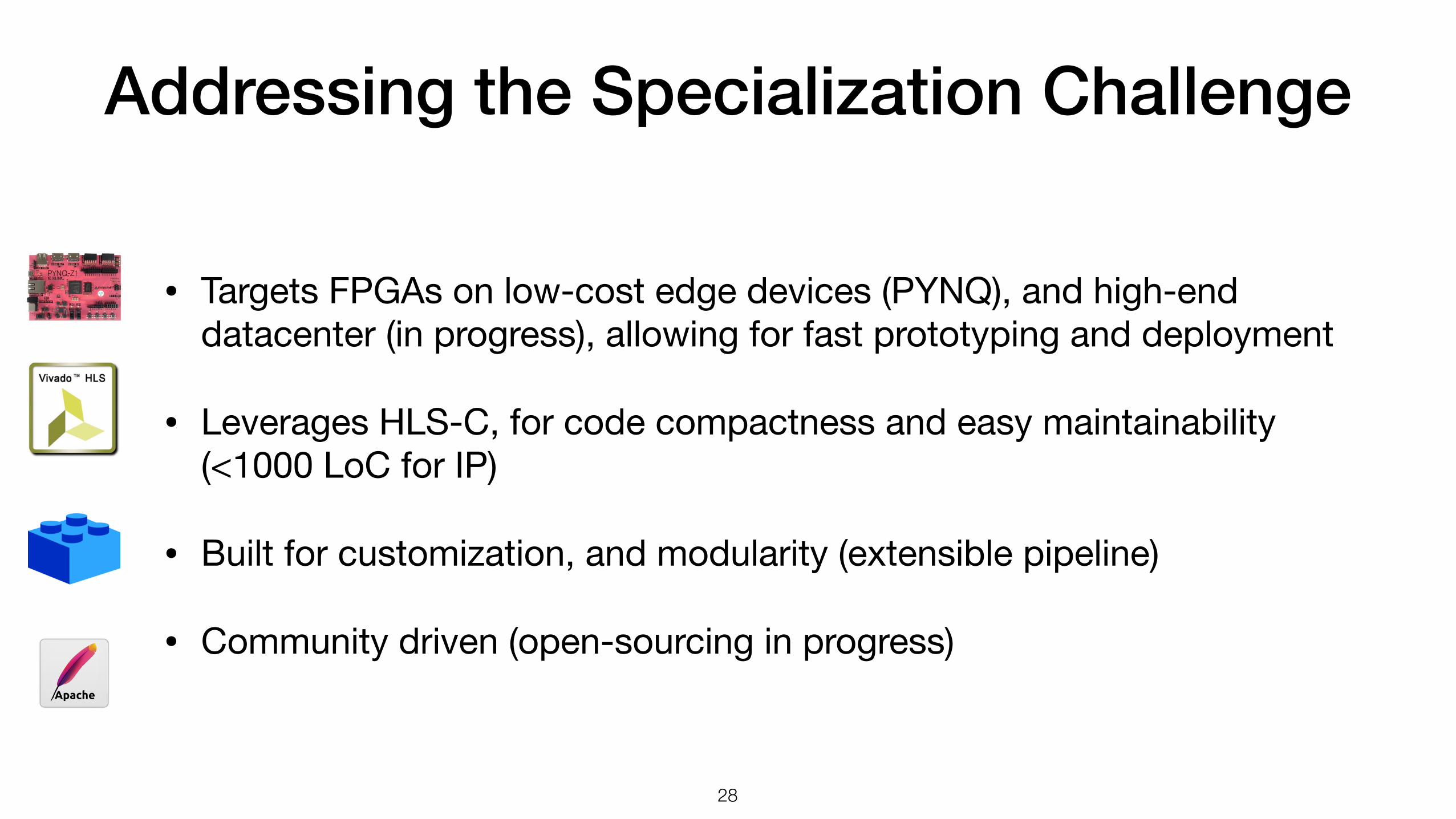
Addressing the Specialization Challenge
• Targets FPGAs on low-cost edge devices (PYNQ), and high-end datacenter (in progress), allowing for fast prototyping and deployment
• Leverages HLS-C, for code compactness and easy maintainability (<1000 LoC for IP)
• Built for customization, and modularity (extensible pipeline)
• Community driven (open-sourcing in progress)
!28

VTA Features
• Customizable tensor core, memory subsystem and data types based on bandwidth, storage and accuracy needs
• Flexible CISC/RISC ISA for expressive and compact code
• Access-execute decoupling for memory latency hiding
!29

Customization
!30
Tensor Intrinsic
x8
8
8
8x
32
1
16
32vs.
Memory Subsystem
vs.
Hardware Datatype
<16 x i8> vs. <32 x i4>
Operator Support
{ADD, MUL, SHL, MAX} {ADD, SHL, MAX}vs.
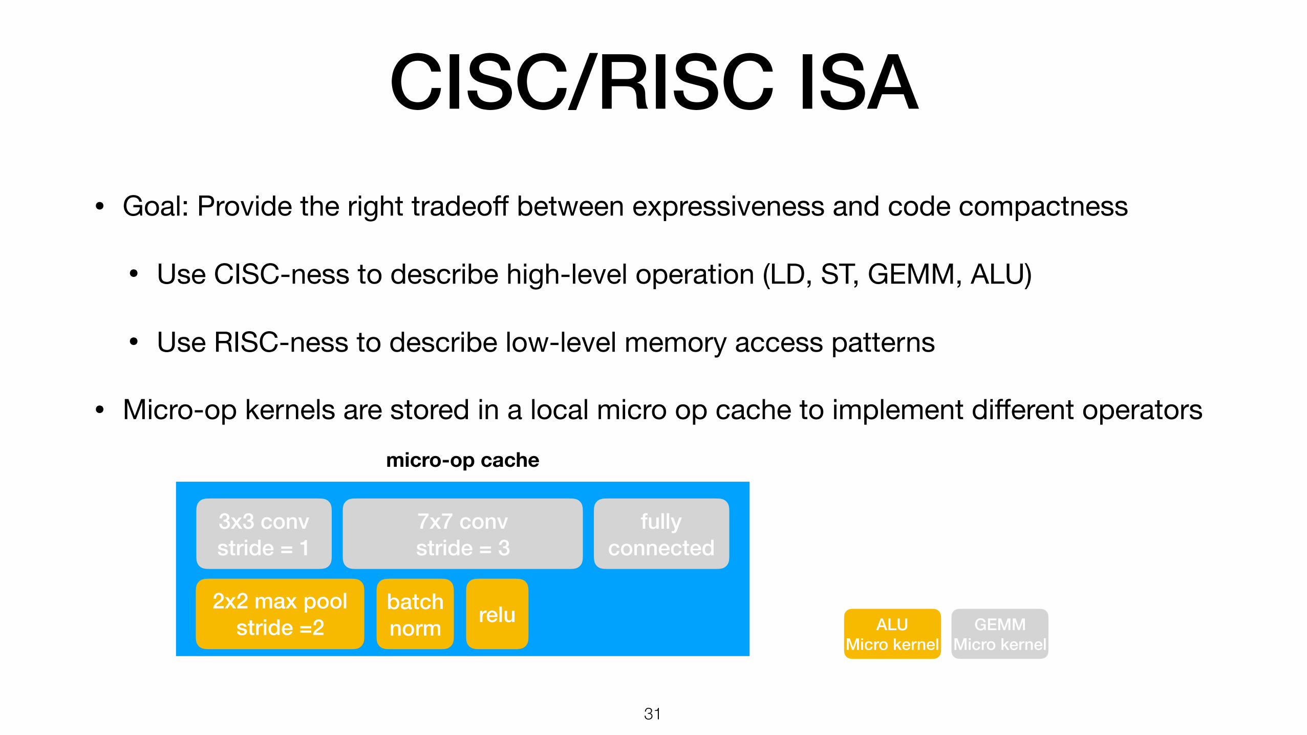
CISC/RISC ISA• Goal: Provide the right tradeoff between expressiveness and code compactness
• Use CISC-ness to describe high-level operation (LD, ST, GEMM, ALU)
• Use RISC-ness to describe low-level memory access patterns
• Micro-op kernels are stored in a local micro op cache to implement different operators
!31
micro-op cache
3x3 conv stride = 1
7x7 conv stride = 3
2x2 max pool stride =2
batch norm
fully connected
GEMM Micro kernel
ALU Micro kernel
relu

Latency Hiding• How do keep computation resources (GEMM) busy:
• Without latency hiding, we are wasting compute/memory resources
• By exploiting pipeline parallelism, we can hide memory latency
LD GEMM LD GEMM LD GEMM LD GEMM ST
LD
GEMM
LD
GEMM
LD
GEMM
LD
GEMM
ST
execution savings
!32
HW
Pip
elin
e

Latency Hiding
LD
GEMM
LD
GEMM
LD
GEMM
LD
GEMM
ST
execution savings
!33
HW
Pip
elin
e
• Pipeline parallelism requirements:
• Concurrent tasks need to access non-overlapping regions of memory
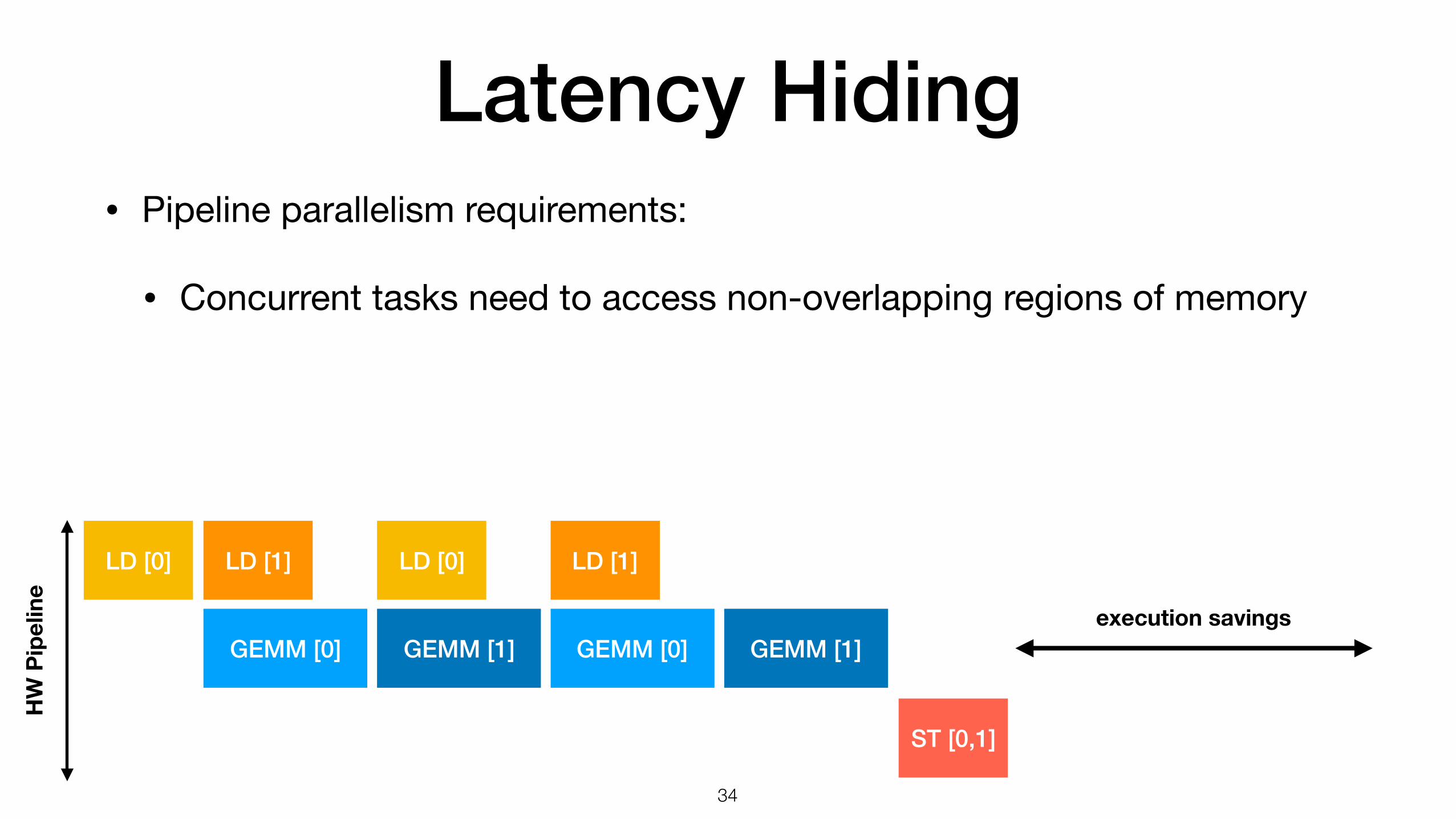
Latency Hiding• Pipeline parallelism requirements:
• Concurrent tasks need to access non-overlapping regions of memory
LD [0]
GEMM [0]
LD [1]
GEMM [1]
LD [0]
GEMM [0]
LD [1]
GEMM [1]
ST [0,1]
execution savings
!34
HW
Pip
elin
e

Latency Hiding• Pipeline parallelism requirements:
• Concurrent tasks need to access non-overlapping regions of memory
• Data dependences need to be explicit!
LD [0]
GEMM [0]
LD [1]
GEMM [1]
LD [0]
GEMM [0]
LD [1]
GEMM [1]
ST [0,1]
execution savings
!35
HW
Pip
elin
e

Latency Hiding• We want to enforce read-after-write (RAW) dependences
LD [0]
EX [0]
LD [1]
EX [1]
LD [0]
EX [0]
LD [1]
EX [1]
ST [0,1]
Without RAW dependence tracking, operations execute as soon as the stage is idle.
!36

Latency Hiding• We want to enforce read-after-write (RAW) dependences
LD [0]
GEMM [0]
LD [1]
GEMM [1]
LD [0]
GEMM [0]
LD [1]
GEMM [1]
ST [0,1]Legend:
RAW dependence:
!37

Latency Hiding• We want to enforce read-after-write (RAW) dependences
• AND we want to enforce write-after-read (WAR) dependences
LD [0]
GEMM [0]
LD [1]
GEMM [1]
LD [0]
GEMM [0]
LD [1]
GEMM [1]
ST [0,1]Legend:
RAW dependence:
We are overwriting data in partition 0 before GEMM has finished consuming data from the first LD!
!38

Latency Hiding• We want to enforce read-after-write (RAW) dependences
• AND we want to enforce write-after-read (WAR) dependences
LD [0]
GEMM [0]
LD [1]
GEMM [1]
LD [0]
GEMM [0]
LD [1]
GEMM [1]
ST [0,1]Legend:
RAW dependence:
WAR dependence:
!39

Latency HidingTakeaway: work partitioning and explicit dependence graph execution (EDGE) unlocks pipeline parallelism to hide the latency of memory accesses
LD [0]
GEMM [0]
LD [1]
GEMM [1]
LD [0]
GEMM [0]
LD [1]
GEMM [1]
ST [0,1]Legend:
RAW dependence:
WAR dependence:
!40

VTA Design Overview
!41
MEMORY LOADUNIT
MEMORY STOREUNIT
DRAM
MICRO-OP SRAM
ACTIVATION SRAM
KERNEL SRAM
LOAD BUFFER STORE BUFFER
REGISTER FILE
GEMM
V_ALU
LOAD→EXE Q
EXE→LOAD Q
EXE→LOAD Q
STORE→EXE Q
INSTRUCTION FETCH
LOAD Q COMPUTE Q
COMPUTE
STORE Q
cont
rolle
r

!42
DRAM
INSTRUCTION FETCH
LOAD Q COMPUTE Q STORE Q
MEMORY LOADUNIT
MEMORY STOREUNIT
DRAM
MICRO-OP SRAM
ACTIVATION SRAM
KERNEL SRAM
LOAD BUFFER STORE BUFFER
REGISTER FILE
GEMM
V_ALU
LOAD→EXE Q
EXE→LOAD Q
EXE→LOAD Q
STORE→EXE Q
INSTRUCTION FETCH
LOAD Q COMPUTE Q
COMPUTE
STORE Q
cont
rolle
r
VTA Design
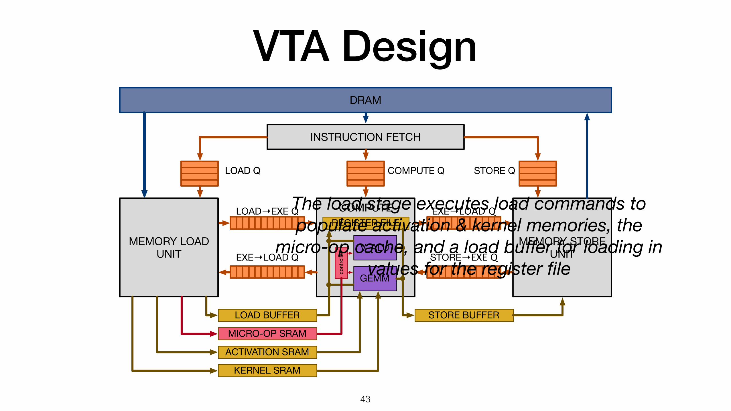
Instruction fetch stage fetches high-level instructions from DRAM, decodes them, and pushes commands to the relevant queue (LD, EX, ST)
VTA Design
!43
MEMORY LOADUNIT
MEMORY STOREUNIT
DRAM
MICRO-OP SRAM
ACTIVATION SRAM
KERNEL SRAM
LOAD BUFFER STORE BUFFER
REGISTER FILE
GEMM
V_ALU
LOAD→EXE Q
EXE→LOAD Q
EXE→LOAD Q
STORE→EXE Q
INSTRUCTION FETCH
LOAD Q COMPUTE Q
COMPUTE
STORE Q
cont
rolle
r
MEMORY LOADUNIT
DRAM
MICRO-OP SRAM
ACTIVATION SRAM
KERNEL SRAM
LOAD BUFFER
LOAD Q
The load stage executes load commands to populate activation & kernel memories, the
micro-op cache, and a load buffer for loading in values for the register file

VTA Design
!44
MEMORY LOADUNIT
MEMORY STOREUNIT
DRAM
MICRO-OP SRAM
ACTIVATION SRAM
KERNEL SRAM
LOAD BUFFER STORE BUFFER
REGISTER FILE
GEMM
V_ALU
LOAD→EXE Q
EXE→LOAD Q
EXE→LOAD Q
STORE→EXE Q
INSTRUCTION FETCH
LOAD Q COMPUTE Q
COMPUTE
STORE Q
cont
rolle
rMICRO-OP SRAM
ACTIVATION SRAM
KERNEL SRAM
LOAD BUFFER STORE BUFFER
REGISTER FILE
GEMM
V_ALU
COMPUTE Q
COMPUTE
cont
rolle
r
Compute stage executes compute commands to perform vector ALU operations or GEMM operations to update the register file according to micro-coded kernels

VTA Design
!45
MEMORY LOADUNIT
MEMORY STOREUNIT
DRAM
MICRO-OP SRAM
ACTIVATION SRAM
KERNEL SRAM
LOAD BUFFER STORE BUFFER
REGISTER FILE
GEMM
V_ALU
LOAD→EXE Q
EXE→LOAD Q
EXE→LOAD Q
STORE→EXE Q
INSTRUCTION FETCH
LOAD Q COMPUTE Q
COMPUTE
STORE Q
cont
rolle
r
MEMORY STOREUNIT
DRAM
STORE BUFFER
STORE Q
Memory store stage executes store commands to store flushed register file
values back to DRAM from the store buffer

VTA Design
!46
MEMORY LOADUNIT
MEMORY STOREUNIT
DRAM
MICRO-OP SRAM
ACTIVATION SRAM
KERNEL SRAM
LOAD BUFFER STORE BUFFER
REGISTER FILE
GEMM
V_ALU
LOAD→EXE Q
EXE→LOAD Q
EXE→LOAD Q
STORE→EXE Q
INSTRUCTION FETCH
LOAD Q COMPUTE Q
COMPUTE
STORE Q
cont
rolle
r
MEMORY LOADUNIT
MEMORY STOREUNIT
LOAD→EXE Q
EXE→LOAD Q
EXE→LOAD Q
STORE→EXE Q
COMPUTE
Stages communicate via dependence token queues to indicate that they may proceed to execute the
command they’re about to work on

VTA Design
!47
MEMORY LOADUNIT
MEMORY STOREUNIT
DRAM
MICRO-OP SRAM
ACTIVATION SRAM
KERNEL SRAM
LOAD BUFFER STORE BUFFER
REGISTER FILE
GEMM
V_ALU
LOAD→EXE Q
EXE→LOAD Q
EXE→LOAD Q
STORE→EXE Q
INSTRUCTION FETCH
LOAD Q COMPUTE Q
COMPUTE
STORE Q
cont
rolle
r
MEMORY LOADUNIT
MEMORY STOREUNIT
MICRO-OP SRAM
ACTIVATION SRAM
KERNEL SRAM
LOAD BUFFER STORE BUFFER
REGISTER FILE
GEMM
V_ALU
COMPUTE
cont
rolle
r
Memories that connect pipeline stages follow a strict single producer, single consumer rule (fan-in=1, fan-out=1).
This enables data flow execution, and makes this design modular.

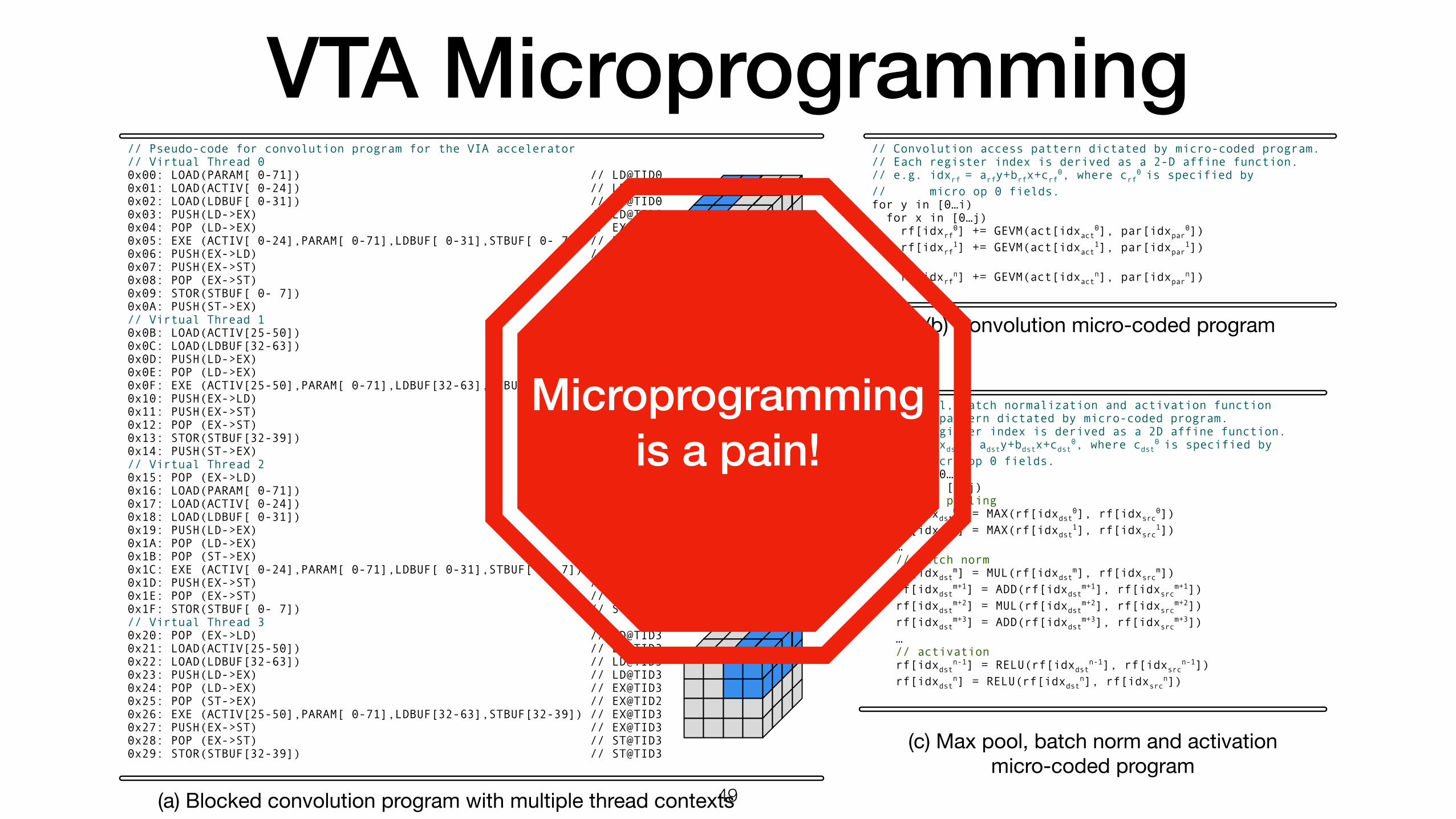
// Pseudo-code for convolution program for the VIA accelerator// Virtual Thread 00x00: LOAD(PARAM[ 0-71]) // LD@TID00x01: LOAD(ACTIV[ 0-24]) // LD@TID00x02: LOAD(LDBUF[ 0-31]) // LD@TID00x03: PUSH(LD->EX) // LD@TID00x04: POP (LD->EX) // EX@TID00x05: EXE (ACTIV[ 0-24],PARAM[ 0-71],LDBUF[ 0-31],STBUF[ 0- 7]) // EX@TID00x06: PUSH(EX->LD) // EX@TID00x07: PUSH(EX->ST) // EX@TID00x08: POP (EX->ST) // ST@TID00x09: STOR(STBUF[ 0- 7]) // ST@TID00x0A: PUSH(ST->EX) // ST@TID0// Virtual Thread 10x0B: LOAD(ACTIV[25-50]) // LD@TID10x0C: LOAD(LDBUF[32-63]) // LD@TID10x0D: PUSH(LD->EX) // LD@TID10x0E: POP (LD->EX) // EX@TID10x0F: EXE (ACTIV[25-50],PARAM[ 0-71],LDBUF[32-63],STBUF[32-39]) // EX@TID10x10: PUSH(EX->LD) // EX@TID10x11: PUSH(EX->ST) // EX@TID10x12: POP (EX->ST) // ST@TID10x13: STOR(STBUF[32-39]) // ST@TID10x14: PUSH(ST->EX) // ST@TID1// Virtual Thread 20x15: POP (EX->LD) // LD@TID20x16: LOAD(PARAM[ 0-71]) // LD@TID20x17: LOAD(ACTIV[ 0-24]) // LD@TID20x18: LOAD(LDBUF[ 0-31]) // LD@TID20x19: PUSH(LD->EX) // LD@TID20x1A: POP (LD->EX) // EX@TID20x1B: POP (ST->EX) // EX@TID20x1C: EXE (ACTIV[ 0-24],PARAM[ 0-71],LDBUF[ 0-31],STBUF[ 0- 7]) // EX@TID20x1D: PUSH(EX->ST) // EX@TID20x1E: POP (EX->ST) // ST@TID20x1F: STOR(STBUF[ 0- 7]) // ST@TID2// Virtual Thread 30x20: POP (EX->LD) // LD@TID30x21: LOAD(ACTIV[25-50]) // LD@TID30x22: LOAD(LDBUF[32-63]) // LD@TID30x23: PUSH(LD->EX) // LD@TID30x24: POP (LD->EX) // EX@TID30x25: POP (ST->EX) // EX@TID20x26: EXE (ACTIV[25-50],PARAM[ 0-71],LDBUF[32-63],STBUF[32-39]) // EX@TID30x27: PUSH(EX->ST) // EX@TID30x28: POP (EX->ST) // ST@TID30x29: STOR(STBUF[32-39]) // ST@TID3
// Convolution access pattern dictated by micro-coded program.// Each register index is derived as a 2-D affine function.// e.g. idxrf = arfy+brfx+crf
0, where crf0 is specified by
// micro op 0 fields.for y in [0…i) for x in [0…j) rf[idxrf
0] += GEVM(act[idxact0], par[idxpar
0]) rf[idxrf
1] += GEVM(act[idxact1], par[idxpar
1]) … rf[idxrf
n] += GEVM(act[idxactn], par[idxpar
n])
(b) Convolution micro-coded program
// Max-pool, batch normalization and activation function// access pattern dictated by micro-coded program.// Each register index is derived as a 2D affine function.// e.g. idxdst = adsty+bdstx+cdst
0, where cdst0 is specified by
// micro op 0 fields.for y in [0…i) for x in [0…j) // max pooling rf[idxdst
0] = MAX(rf[idxdst0], rf[idxsrc
0]) rf[idxdst
1] = MAX(rf[idxdst1], rf[idxsrc
1]) … // batch norm rf[idxdst
m] = MUL(rf[idxdstm], rf[idxsrc
m]) rf[idxdst
m+1] = ADD(rf[idxdstm+1], rf[idxsrc
m+1]) rf[idxdst
m+2] = MUL(rf[idxdstm+2], rf[idxsrc
m+2]) rf[idxdst
m+3] = ADD(rf[idxdstm+3], rf[idxsrc
m+3]) … // activation rf[idxdst
n-1] = RELU(rf[idxdstn-1], rf[idxsrc
n-1]) rf[idxdst
n] = RELU(rf[idxdstn], rf[idxsrc
n])
(c) Max pool, batch norm and activationmicro-coded program
(a) Blocked convolution program with multiple thread contexts
VTA Microprogramming
!48
// Pseudo-code for convolution program for the VIA accelerator// Virtual Thread 00x00: LOAD(PARAM[ 0-71]) // LD@TID00x01: LOAD(ACTIV[ 0-24]) // LD@TID00x02: LOAD(LDBUF[ 0-31]) // LD@TID00x03: PUSH(LD->EX) // LD@TID00x04: POP (LD->EX) // EX@TID00x05: EXE (ACTIV[ 0-24],PARAM[ 0-71],LDBUF[ 0-31],STBUF[ 0- 7]) // EX@TID00x06: PUSH(EX->LD) // EX@TID00x07: PUSH(EX->ST) // EX@TID00x08: POP (EX->ST) // ST@TID00x09: STOR(STBUF[ 0- 7]) // ST@TID00x0A: PUSH(ST->EX) // ST@TID0// Virtual Thread 10x0B: LOAD(ACTIV[25-50]) // LD@TID10x0C: LOAD(LDBUF[32-63]) // LD@TID10x0D: PUSH(LD->EX) // LD@TID10x0E: POP (LD->EX) // EX@TID10x0F: EXE (ACTIV[25-50],PARAM[ 0-71],LDBUF[32-63],STBUF[32-39]) // EX@TID10x10: PUSH(EX->LD) // EX@TID10x11: PUSH(EX->ST) // EX@TID10x12: POP (EX->ST) // ST@TID10x13: STOR(STBUF[32-39]) // ST@TID10x14: PUSH(ST->EX) // ST@TID1// Virtual Thread 20x15: POP (EX->LD) // LD@TID20x16: LOAD(PARAM[ 0-71]) // LD@TID20x17: LOAD(ACTIV[ 0-24]) // LD@TID20x18: LOAD(LDBUF[ 0-31]) // LD@TID20x19: PUSH(LD->EX) // LD@TID20x1A: POP (LD->EX) // EX@TID20x1B: POP (ST->EX) // EX@TID20x1C: EXE (ACTIV[ 0-24],PARAM[ 0-71],LDBUF[ 0-31],STBUF[ 0- 7]) // EX@TID20x1D: PUSH(EX->ST) // EX@TID20x1E: POP (EX->ST) // ST@TID20x1F: STOR(STBUF[ 0- 7]) // ST@TID2// Virtual Thread 30x20: POP (EX->LD) // LD@TID30x21: LOAD(ACTIV[25-50]) // LD@TID30x22: LOAD(LDBUF[32-63]) // LD@TID30x23: PUSH(LD->EX) // LD@TID30x24: POP (LD->EX) // EX@TID30x25: POP (ST->EX) // EX@TID20x26: EXE (ACTIV[25-50],PARAM[ 0-71],LDBUF[32-63],STBUF[32-39]) // EX@TID30x27: PUSH(EX->ST) // EX@TID30x28: POP (EX->ST) // ST@TID30x29: STOR(STBUF[32-39]) // ST@TID3
// Convolution access pattern dictated by micro-coded program.// Each register index is derived as a 2-D affine function.// e.g. idxrf = arfy+brfx+crf
0, where crf0 is specified by
// micro op 0 fields.for y in [0…i) for x in [0…j) rf[idxrf
0] += GEVM(act[idxact0], par[idxpar
0]) rf[idxrf
1] += GEVM(act[idxact1], par[idxpar
1]) … rf[idxrf
n] += GEVM(act[idxactn], par[idxpar
n])
(b) Convolution micro-coded program
// Max-pool, batch normalization and activation function// access pattern dictated by micro-coded program.// Each register index is derived as a 2D affine function.// e.g. idxdst = adsty+bdstx+cdst
0, where cdst0 is specified by
// micro op 0 fields.for y in [0…i) for x in [0…j) // max pooling rf[idxdst
0] = MAX(rf[idxdst0], rf[idxsrc
0]) rf[idxdst
1] = MAX(rf[idxdst1], rf[idxsrc
1]) … // batch norm rf[idxdst
m] = MUL(rf[idxdstm], rf[idxsrc
m]) rf[idxdst
m+1] = ADD(rf[idxdstm+1], rf[idxsrc
m+1]) rf[idxdst
m+2] = MUL(rf[idxdstm+2], rf[idxsrc
m+2]) rf[idxdst
m+3] = ADD(rf[idxdstm+3], rf[idxsrc
m+3]) … // activation rf[idxdst
n-1] = RELU(rf[idxdstn-1], rf[idxsrc
n-1]) rf[idxdst
n] = RELU(rf[idxdstn], rf[idxsrc
n])
(c) Max pool, batch norm and activationmicro-coded program
(a) Blocked convolution program with multiple thread contexts
VTA Microprogramming
!49
Microprogramming is a pain!

Building a deep learning accelerator compiler stack in TVM
• TVM: An end-to-end compiler & optimization framework for diverse hardware
Chen, Moreau, Jiang, Shen, Yan, Wang, Hu, Ceze, Guestrin and KrishnamurthyTVM: End-to-end Compilation Stack for Deep Learning SysML 2018 (1 of 6 invited talk) !50

Addressing the Programmability Challenge
VTA FPGA Design
Runtime & JIT Compiler
FPGA/SoC Drivers
RPC Layer
TVM Compiler
NNVM Graph
High-Level Deep Learning Framework
!51
TVM DSL allows for separation of schedule and algorithm
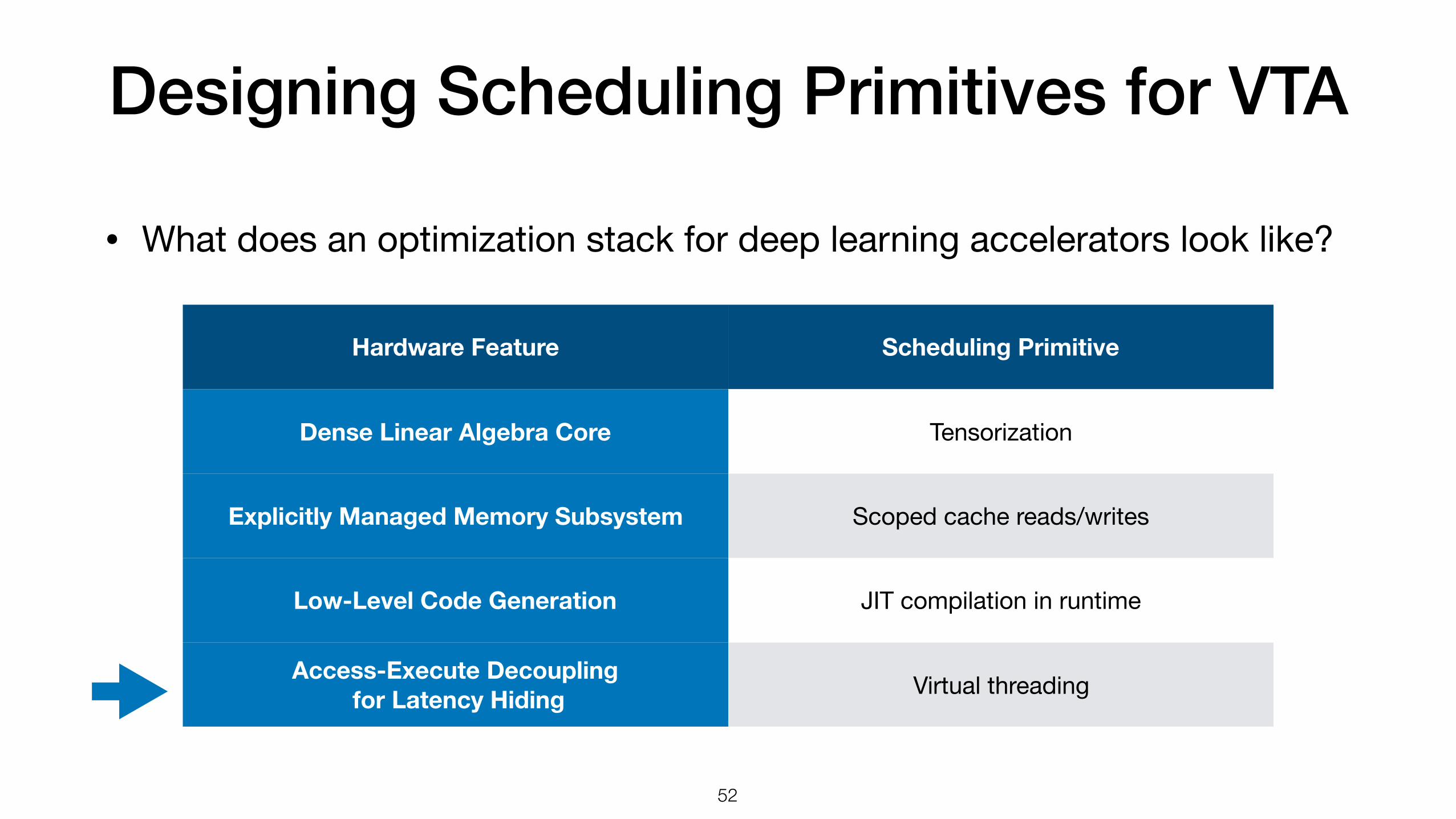
Designing Scheduling Primitives for VTA
• What does an optimization stack for deep learning accelerators look like?
Hardware Feature Scheduling Primitive
Dense Linear Algebra Core Tensorization
Explicitly Managed Memory Subsystem Scoped cache reads/writes
Low-Level Code Generation JIT compilation in runtime
Access-Execute Decoupling for Latency Hiding Virtual threading
!52

Virtual Threading• How do we take advantage of pipeline parallelism with virtual threading?
Execution Phase 1 Execution Phase 2
Load Stage
GEMM Stage
Store Stage
Hardware-centric view: pipeline execution
LD
EX
LD
EX
LD
EX
LD
EX
ST
LD
EX
LD
EX
LD
EX
LD
EX
ST
!53

Virtual Threading• How do we take advantage of pipeline parallelism with virtual threading?
Execution Phase 1 Execution Phase 2
Software-centric view: threaded execution
LD
EX
LD
EX
LD
EX
LD
EX
ST
LD
EX
LD
EX
LD
EX
LD
EX
ST
!54
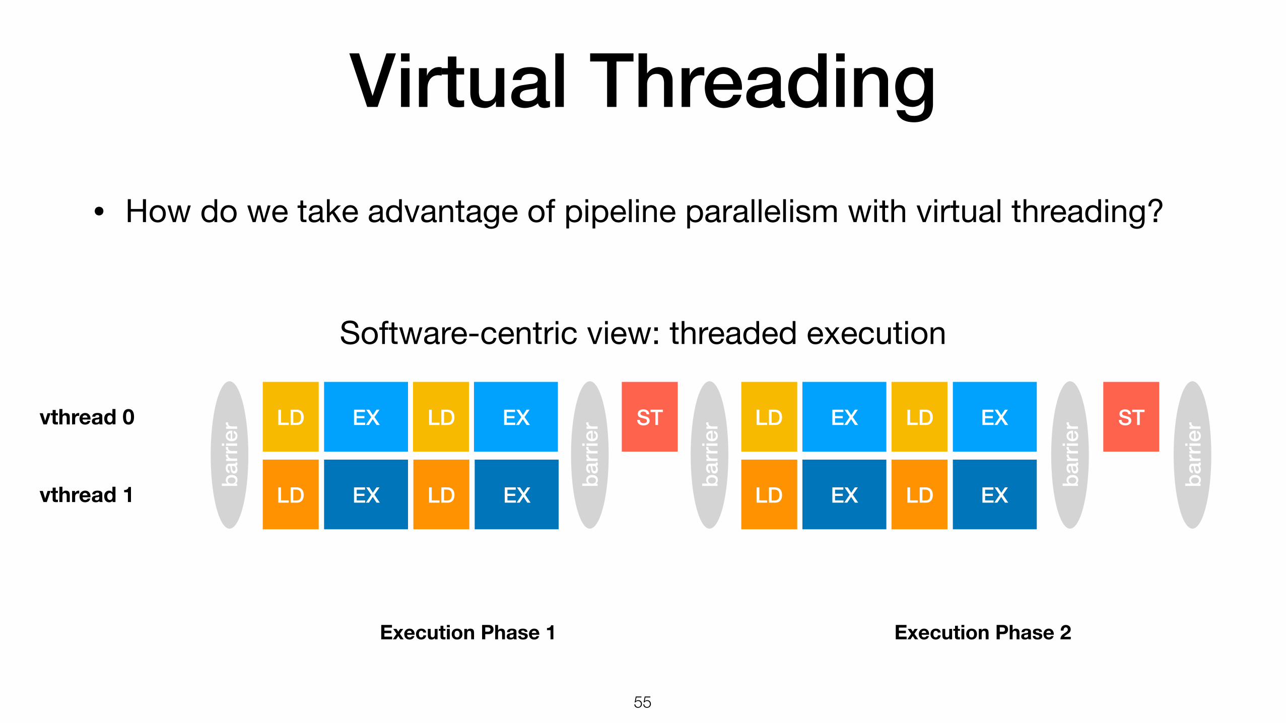
Virtual Threading• How do we take advantage of pipeline parallelism with virtual threading?
Execution Phase 1 Execution Phase 2
Software-centric view: threaded execution
LD EX
LD EX
LD EX
LD EX
ST LD EX
LD EX
LD EX
LD EX
ST
barri
er
barri
er
barri
er
barri
er
barri
er
vthread 0
vthread 1
!55

Virtual Threading
Execution Phase 1 Execution Phase 2
Software-centric view: threaded execution
LD EX
LD EX
LD EX
LD EX
ST LD EX
LD EX
LD EX
LD EX
ST
barri
er
barri
er
barri
er
barri
er
barri
er
vthread 0
vthread 1
• Benefit #1: dependences are automatically inserted between successive stages within each virtual threadLegend:
RAW dependence:
WAR dependence:
!56

Virtual Threading
Execution Phase 1 Execution Phase 2
Software-centric view: threaded execution
LD EX
LD EX
LD EX
LD EX
ST LD EX
LD EX
LD EX
LD EX
ST
barri
er
barri
er
barri
er
barri
er
barri
er
vthread 0
vthread 1
• Benefit #1: dependences are automatically inserted between successive stages within each virtual thread
• Benefit #2: barriers insert dependences between execution stages to guarantee sequential consistency
Legend:
RAW dependence:
WAR dependence:
!57

Virtual ThreadingFinal step: virtual thread lowering into a single instruction stream
LD EXLD EX LD EXLD EX ST… …
push dependence to consumer stage
push dependence to producer stage
pop dependence from producer stage
pop dependence from consumer stage
Legend
MEMORY LOADUNIT
MEMORY STOREUNIT
LOAD→EXE Q
EXE→LOAD Q
EXE→LOAD Q
STORE→EXE Q
COMPUTE
Push and pop commands dictate how to interact with the hardware dependence queues

Programming for VTA in TVM1. How do we partition work and explicitly manage on-chip memories?
2. How do we take advantage of tensorization?
3. How do we take advantage of virtual threading?
W
H
CI
W
H
CI
❌ not enough SRAM! ✅ fits in SRAM
= x
LD GEMM
LD GEMM
LD GEMM
LD GEMM
ST LD GEMM
LD GEMM
LD GEMM
LD GEMM
ST
barri
er
barri
er
barri
er
barri
er
barri
er
!59

TVM Scheduling Primitives1. How do we partition work and explicitly manage on-chip memories?
2. How do we take advantage of tensorization?
3. How do we take advantage of virtual threading?
!60
// Tileyo, xo, yi, xi = s[OUT].tile(y, x, 4, 4)// Cache readINP_L = s.cache_read(INP, vta.act, [OUT])s[INP_L].compute_at(s[OUT], xo)
// Tensorizes[OUT_L].tensorize(ni)
// Virtual Threadingtx, co = s[OUT_L].split(co, factor=2)s[OUT_L].bind(tx, thread_axis(“cthread”))

Full Stack Evaluation (TVM)• Full evaluation on PYNQ FPGA board
!61
TVM can offload most convolution operations to the FPGA (40x speedup on off-loadable layers)
TVM can exploit latency hiding mechanisms to improve throughput.
Utilization improves from at best 52% to 74%.

Resources
• Build your own simple VTA accelerator: https://gitlab.cs.washington.edu/cse599s/lab1
• TVM Tutorial for VTA to be released
• Looking for alpha users of the full VTA open source design
