hardware-in-the-loop simulation of power electronic...

1146 IEEE TRANSACTIONS ON INDUSTRIAL ELECTRONICS, VOL. 57, NO. 4, APRIL 2010

Hardware-in-the-Loop Simulation ofPower Electronic Systems Using

Adaptive DiscretizationM. Omar Faruque, Member, IEEE, and Venkata Dinavahi, Senior Member, IEEE

Abstract—This paper presents the hardware-in-the-loop (HIL)simulation of power electronic systems using a unique adap-tive discretization technique based on the input of the sys-tem, where the coefficient matrices and system equations arechanged while the simulation is running. The voltage-source-converter (VSC)-based HVDC system is used as a case study.Two z-transform-based discretization techniques, known as thestep-invariant transformation (SIT) and the ramp-invariant trans-formation, and one of their derivative time-shifted SIT are ap-plied for simulating the VSC-HVDC system. Discrete switchingsynchronization algorithms are used to accommodate the asyn-chronous events that take place in between two discrete simulationpoints. The HIL simulation is implemented using an off-the-shelfPC cluster interfaced with a digital controller. The simulator andthe controller are connected through I/O ports, which facilitate theexchange of analog and digital signals. A 4-kW VSC-HVDC exper-imental setup is used to validate the simulation results, using thesame digital controller as that in the HIL simulation to supply thenecessary gate pulses for the experimental VSCs. A comparativestudy of the results obtained through offline, HIL simulation, andthe experiment is presented.

Index Terms—Hardware-in-the-loop (HIL) simulation, HVDCtransmission, power system transients, pulsewidth-modulatedconverters, real-time systems, z transforms.

I. INTRODUCTION

HARDWARE-IN-THE-LOOP (HIL) simulation has be-come a crucial stage in the design and development of

digital controllers for a power electronic apparatus used atdifferent power and voltage levels in a power system. Appli-cations of this technology [1]–[7] include flexible ac transmis-sion systems and HVDC at the transmission level, distributedgeneration and power quality regulation at the distributionlevel, and variable speed industrial drives at the utilizationlevel. A comprehensive evaluation of all modes of operation ofthe controller under realistic system conditions is the primaryrequirement for the controller to be effective once it is installedin the field. HIL simulation offers the advantages of reduced

Manuscript received December 25, 2008; revised November 2, 2009. Firstpublished November 24, 2009; current version published March 10, 2010.

M. Omar Faruque was with the Department of Electrical and ComputerEngineering, University of Alberta, Edmonton, AB T6G 2V4, Canada. Heis now with The Center for Advanced Power Systems, The Florida StateUniversity, Tallahassee, FL 32310 USA (e-mail: [email protected]).

V. Dinavahi is with the Department of Electrical and Computer Engi-neering, University of Alberta, Edmonton, AB T6G 2V4, Canada (e-mail:[email protected]).

Color versions of one or more of the figures in this paper are available onlineat http://ieeexplore.ieee.org.

Digital Object Identifier 10.1109/TIE.2009.2036647

cost, fast repeatability of the tests, and the ability to subject thecontroller to risky contingency situations.

As the name implies, in HIL simulation, a part of the systemis modeled and simulated in real time, while the remainder isthe actual hardware, connected in closed loop through variousI/O interfaces such as analog-to-digital (A/D) and digital-to-analog converters, and signal conditioning equipment. Thesimulation can be controlled by user-defined external inputs,e.g., closing and opening of switches to connect the componentsin the modeled system. HIL simulation can be of two kinds:controller HIL (C-HIL) simulation or signal HIL and powerHIL (P-HIL) simulation. In C-HIL simulation, the power sys-tem, including the power electronic converters, is representedby a real-time model, while the digital controller is the deviceunder test connected in closed loop with that model. Thismethod is also known as rapid controller prototyping. There isno real power transfer in this method. The controller takes in thesampled voltages and currents from the simulator and providescontrol inputs in the form of switching signals. In contrast, inP-HIL simulation, a part of the power system is external to thesimulator, thus requiring a transfer of real power to the externalhardware.

In both types of HIL simulation, the use of an accu-rate discrete-time system model is paramount. Therefore, themethod used to discretize the continuous-time system modelis a key factor influencing simulation accuracy. Until now,most of the literature related to C-HIL simulation has focusedon the accounting of discrete switching signals coming fromthe controller in a fixed-time-step simulation process [8]–[13].However, the discretization methods used were the same asthose used in offline Electromagnetic Transients Program sim-ulation [14] such as the trapezoidal rule (TR). Although thismethod has been widely used, it can still cause errors in somecases due to spurious numerical oscillations [15]. In addition,at larger time steps, it can cause frequency warping and deviatefrom the actual response.

Various z-transform-based discretization techniques havebeen applied earlier for offline electromagnetic transient sim-ulation [16], [17]. In those applications, a single discretizationmethod is chosen for the entire simulation even though theperformance of the discretization algorithm is found to varywith inputs. The accuracy of the simulation greatly depends onthe selection of proper approximation (s to z domain) for a par-ticular type of input to the system. In this paper, we propose anadaptive application of z-transform-based discretization meth-ods such as step-invariant transformation (SIT), ramp-invariant

0278-0046/$26.00 © 2010 IEEE

OMAR FARUQUE AND DINAVAHI: HIL SIMULATION OF POWER ELECTRONIC SYSTEMS 1147

transformation (RIT), and time-shifted SIT (TSSIT), hithertoused for digital control and digital filter design [18] for HILsimulation. These methods are adaptive in the sense that theyare excitation- or input-based, i.e., the discretization algorithmis selected based on the type of the system inputs. The methodsare derived based on the assumption of input being held con-stant or being a ramp function for a time step, thereby producingerror-free results if the supplied input to the system matcheswith the input assumed in the algorithm. During transients ordisturbances, the excitation of the system changes abruptly. Theproposed approach in such a situation is to switch to the properdiscretization algorithm at the instant of change in the inputs.This technique represents the inputs correctly and minimizesthe simulation errors, consequently improving the accuracy ofthe simulation due to the best representation of the discrete-time system. The challenge of using more than one discretiza-tion techniques in real-time simulation lies in the changes ofcoefficient matrices which contain time-consuming exponentialterms. In an offline simulation, this is not a problem as theexecution time is not a constraint; however, for real simulation,the simulation must be finished within the assigned time step. Inreal-time simulation, the coefficient matrices are precalculatedfor each discretization technique and switched when necessary.

This paper is organized as follows: In Section II, we presentthe fundamentals on the discrete-time simulation of a systemusing the z-transform-based techniques. In Section III, severalexamples are presented using simple RL and RLC circuitsto compare the performance of these techniques vis-a-vis theTR and the exact solution. Section IV utilizes the adaptive dis-cretization technique to perform a complete HIL simulation ofa voltage source converter (VSC) HVDC system. Offline sim-ulation and experimental implementation were done to verifythe validity of the HIL simulation. In Section V, the three setsof results from the offline simulation, HIL simulation, and theexperiment are analyzed and compared under both steady-stateand transient scenarios. Conclusion is presented in Section VI.

II. z-TRANSFORM-BASED DISCRETIZATION METHODS

Although several discretization techniques [14], [16], [17]are available in the literature, there is no unique, accurate,and stable equivalence between a continuous-time system andits discrete-time counterpart. The most commonly used dis-cretization techniques for electromagnetic transient simulationare based on numerical integration algorithms. However,z-transform-based discretization methods can be used to pro-duce more accurate, stable, and efficient results if they areselected and applied based on the type of input to the system.

z transform is a powerful operational method [18] in discrete-time analysis which considers only the sampled values of afunction y(t), i.e., y(0), y(Δt), y(2Δt), . . ., where Δt is thesampling period. The z transform of a function y(t) (where tis nonnegative) or of a sequence of values of y(kΔt) (where kis zero or a positive integer) is defined as

Y (z) =∞∑

k=0

y(kΔt)z−k

= y(0) + y(Δt)z−1 + y(2Δt)z−2

+ · · · + y(kΔt)z−k + · · · . (1)

Fig. 1. (a) Analog plant. (b) Required digital plant for simulation. (c) Conver-sion to digital plant. (d) Converted digital plant.

Equation (1) implies that the z transform of any continuous-time function can be written in the form of a series, where z−k

indicates the position in time at which the amplitude of thefunction is y(kΔt). The inverse z transform of this sequenceof y(kΔt) will give the values of y(t) at the respective instantsof time. Physical systems, which are linear and time invariant,can be represented as shown in Fig. 1(a) with an input u(t), atransfer function G(s), and an output y(t). However, to performcomputer simulation of this system, its digital equivalent shownin Fig. 1(b) is necessary, where the input is u(kΔt), the transferfunction is G(z), and the output is y(kΔt). If y(t) is theresponse of a system with transfer function G(s) and if itsinput is u(t), digital simulation will yield responses y(kΔt)only at times t = 0,Δt, 2Δt, . . .. However, if the assumptionof variations in inputs between any two consecutive discretepoints does not match with the variation that is present in thereal inputs, the response may not be accurate. If systems arediscretized assuming that the input u(t) varies either as a stepfunction or a ramp function between two discrete instants, theyare known as SIT and RIT, respectively.

Fig. 1(c) shows the conversion using SIT with the corre-sponding discrete-time transfer function G(z) given as

G(z) =z − 1

zZ

[G(s)

s

](2)

which is equivalent to adding a zero-order hold at the beginningof the plant and an A/D converter after the plant. The conversionto G(z) can also be done using RIT which follows

G(z) =[(1 − z−1)2

Δtz−1

]Z

[G(s)s2

]. (3)

These approximations of G(s) yield exact responses onlywhen the input is actually a step function or a ramp function,with changes occurring only at the sample instants. For otherinputs, the approximation will introduce errors in the solution.These errors can be minimized through the careful selection ofalgorithms depending on the type of inputs. The response y(t)of the system can be obtained as

y(t)|t=kΔt = Z−1 [G(z)U(z)] (4)

where U(z) is the z transform of u(t)|t=kΔt.If the s-domain transfer function is strictly proper, the SIT

will introduce at least one pole in the origin, which creates a


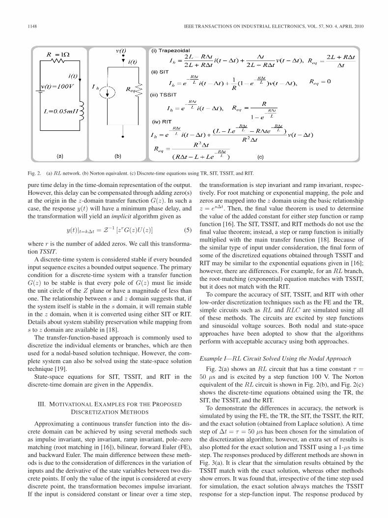
Fig. 2. (a) RL network. (b) Norton equivalent. (c) Discrete-time equations using TR, SIT, TSSIT, and RIT.

pure time delay in the time-domain representation of the output.However, this delay can be compensated through adding zero(s)at the origin in the z-domain transfer function G(z). In such acase, the response y(t) will have a minimum phase delay, andthe transformation will yield an implicit algorithm given as

y(t)|t=kΔt = Z−1 [zrG(z)U(z)] (5)

where r is the number of added zeros. We call this transforma-tion TSSIT.

A discrete-time system is considered stable if every boundedinput sequence excites a bounded output sequence. The primarycondition for a discrete-time system with a transfer functionG(z) to be stable is that every pole of G(z) must lie insidethe unit circle of the Z plane or have a magnitude of less thanone. The relationship between s and z domain suggests that, ifthe system itself is stable in the s domain, it will remain stablein the z domain, when it is converted using either SIT or RIT.Details about system stability preservation while mapping froms to z domain are available in [18].

The transfer-function-based approach is commonly used todiscretize the individual elements or branches, which are thenused for a nodal-based solution technique. However, the com-plete system can also be solved using the state-space solutiontechnique [19].

State-space equations for SIT, TSSIT, and RIT in thediscrete-time domain are given in the Appendix.

III. MOTIVATIONAL EXAMPLES FOR THE PROPOSED

DISCRETIZATION METHODS

Approximating a continuous transfer function into the dis-crete domain can be achieved by using several methods suchas impulse invariant, step invariant, ramp invariant, pole–zeromatching (root matching in [16]), bilinear, forward Euler (FE),and backward Euler. The main difference between these meth-ods is due to the consideration of differences in the variation ofinputs and the derivative of the state variables between two dis-crete points. If only the value of the input is considered at everydiscrete point, the transformation becomes impulse invariant.If the input is considered constant or linear over a time step,

the transformation is step invariant and ramp invariant, respec-tively. For root matching or exponential mapping, the pole andzeros are mapped into the z domain using the basic relationshipz = esΔt. Then, the final value theorem is used to determinethe value of the added constant for either step function or rampfunction [16]. The SIT, TSSIT, and RIT methods do not use thefinal value theorem; instead, a step or ramp function is initiallymultiplied with the main transfer function [18]. Because ofthe similar type of input under consideration, the final form ofsome of the discretized equations obtained through TSSIT andRIT may be similar to the exponential equations given in [16];however, there are differences. For example, for an RL branch,the root-matching (exponential) equation matches with TSSIT,but it does not match with the RIT.

To compare the accuracy of SIT, TSSIT, and RIT with otherlow-order discretization techniques such as the FE and the TR,simple circuits such as RL and RLC are simulated using allof these methods. The circuits are excited by step functionsand sinusoidal voltage sources. Both nodal and state-spaceapproaches have been adopted to show that the algorithmsperform with acceptable accuracy using both approaches.

Example I—RL Circuit Solved Using the Nodal Approach

Fig. 2(a) shows an RL circuit that has a time constant τ =50 μs and is excited by a step function 100 V. The Nortonequivalent of the RL circuit is shown in Fig. 2(b), and Fig. 2(c)shows the discrete-time equations obtained using the TR, theSIT, the TSSIT, and the RIT.

To demonstrate the differences in accuracy, the network issimulated by using the FE, the TR, the SIT, the TSSIT, the RIT,and the exact solution (obtained from Laplace solution). A timestep of Δt = τ = 50 μs has been chosen for the simulation ofthe discretization algorithm; however, an extra set of results isalso plotted for the exact solution and TSSIT using a 1-μs timestep. The responses produced by different methods are shown inFig. 3(a). It is clear that the simulation results obtained by theTSSIT match with the exact solution, whereas other methodsshow errors. It was found that, irrespective of the time step usedfor simulation, the exact solution always matches the TSSITresponse for a step-function input. The response produced by


Fig. 3. Step response (a) for Δt = τ = 50 μs and (b) for Δt = 5τ =250 μs.

SIT is similar to the TSSIT response except that SIT createsone time-step delay in the output. As shown in Fig. 3(b),for a time step of Δt = 5τ = 250 μs, FE does not converge,and the TR shows oscillations even though SIT, TSSIT, andRIT are stable. The TSSIT response again matches with theexact response at both 1 and 250 μs. The oscillation in theTR decays slowly and finally settles to a steady-state value.However, the RIT produces more accurate and stable responsethan the trapezoidal response, and it settles to a steady-statevalue faster than TR without showing any oscillation. Thisconcludes that the proposed methods (SIT, TSSIT, and RIT)can be applied even at larger time steps when the TR fails toresponse accurately.

The same RL circuit is now excited by a sinusoidal voltagewith a frequency of 2 kHz. A time step of Δt = 10 μs was usedto simulate the network using all the methods. The responsesobtained through all these methods are shown in Fig. 4. As canbe seen from Fig. 4, the steady-state response of the networkobtained through TR and RIT closely matches with the exactresponse. The other methods show larger errors. However, ifthe input sinusoidal voltage is changed suddenly, the TSSIT

Fig. 4. Network response at a time step of Δt = 10 μs: (a) For a sinusoidalinput. (b) Zoomed view.

response becomes closer to the exact response, as shown in thezoomed view in Fig. 4(b). It can be concluded that, for a systemwith sinusoidal input, RIT performs closer to the exact solutionand that, if there is any abrupt input change such as during afault, TSSIT would outperform the others.

Example II—RLC Circuit Solved Usingthe State-Space Approach

The use of SIT and RIT in the state-space solution techniquehas long been used in solving electronic circuits [19]. An exam-ple case has been described here to demonstrate the suitabilityand comparative advantage of SIT and RIT over TR for solvingan RLC circuit. A series RLC circuit, shown in Fig. 5, wassolved using the state-space solution technique. The input tothe system is a step function given as

U(t) = 10u(t). (6)

The parameters of the RLC circuit are chosen arbitrarily,keeping in mind that the step response becomes oscillatory with


Fig. 5. (a) RLC network. (b) Step-function input. (c) Equivalent state-space model.

Fig. 6. (a) Step response of an RLC network solved by the state-spacesolution technique with different discretization methods at a time step ofΔt = 50 μs. (b) Zoomed view of the response.

a decaying amplitude. A value of R = 1 Ω, L = 10 mH, andC = 25 μF produces the following state-space equation:

x(t) =[−100 −10040 000 0

]x +

[1000

]u (7)

y = [ 1 1 ]x. (8)

The aforementioned state-space equation can be simulatedusing the discretization algorithms such as TR, SIT, TSSIT,and RIT. The simulation results obtained using a time step of50 μs are shown in Fig. 6. It can be seen that the solutionobtained through the TSSIT method matches accurately with

Fig. 7. (a) Step response of an RLC network solved by the state-spacesolution technique using different discretization methods with a time step ofΔt = 250 μs. (b) Zoomed view of the response.

the exact solution. However, the SIT shows a phase error dueto its inherent delay of one time step. The RIT has been foundto match closely with the trapezoidal method, which was thecase in the nodal approach. However, when the same circuit issimulated using a time step of Δt = 250 μs, it was found thatthe TSSIT method still matches with the exact method, whileRIT and SIT produce errors (Fig. 7). RIT produces less errorthan SIT as SIT suffers from an inherent time-step delay. On theother hand, TR shows a frequency error which is not seen in anyother case. This phenomenon is known as frequency warping,which normally occurs when the TR is used with a large timestep. Case studies show that the type of input plays an important


Fig. 8. Schematic of the VSC-HVDC system used for the HIL simulation and the experimental setup.

role in the accuracy of the simulation results using z-transform-based discretization methods. z transform alone does not con-sider how the input is varied between discrete points; however,algorithms developed based on the variation of inputs betweendiscrete points such as SIT, TSSIT, and RIT produce more accu-rate results if the change in input is taken into account properly.

IV. HIL SIMULATION CASE STUDY: VSC-HVDC SYSTEM

VSC-HVDC is a VSC-based dc transmission technology,where force-commutated switching devices such as gate turn-off thyristors or insulated-gate bipolar transistors (IGBTs) areoperated through a pulsewidth modulation (PWM) scheme.With this technology, it is possible to generate voltages atany magnitude, angle, and frequency (up to a certain limit)through changes in the control and PWM scheme. Because ofthe controllability of the VSCs, active power can be transferredfrom one side to another, and reactive power can be generatedindependently.

Fig. 8 shows the schematic diagram of the VSC-HVDC testsystem and its controller used for the HIL simulation and theexperiment. It mainly consists of two ac sources, phase reactorson both sides, two converters, and a dc link. The two ac suppliesof the network are represented by three-phase Y-connected andgrounded infinite sources with no source impedance. The twoconverters, with one operating as an inverter and the otheras a rectifier, are built of IGBTs and connected back-to-backthrough a dc-link capacitor.

A. Operation of the VSC-HVDC System

The converters used in a VSC-HVDC system can be consid-ered as variable voltage sources as they are capable of gener-

ating voltages of any magnitude, phase angle, and frequency.With respect to the dc-link voltage Vdc, the instantaneousvoltage at the terminal of converter 2 V2i can be given as

V2i = KmaVdc sin(ωt + δ) (9)

where K is a constant whose value depends on the modulationscheme, ma is the modulation index defined by the ratio ofthe peak value of the modulating wave to the peak value ofthe carrier wave, ω is the fundamental frequency, and δ is thephase shift with respect to the ac terminal voltage. The phase-shift angle δ and the modulation index ma can be controlledto generate any combination of voltage magnitude and phaseangle (limited by the dc voltage).

B. Control of the VSC-HVDC System

The most important aspect of a VSC-HVDC is its abilityto control active and reactive power independently. The activepower is controlled by controlling the dc-link voltage, and thereactive power is controlled by changing the ac voltages atthe converter terminals. Using the abc−αβ−dq transformationsand a vector control technique [22], the control schemes forboth converters were developed. The control schemes for thetwo converters are similar with small differences in the deriva-tion of the reference signals. The decoupled control schemefor VSC 1 is given in Fig. 9. The objective of the controlscheme is to determine the required ma and δ for any particularlevel of power transfer in such a way that any change in thereference power level will be reflected through a change in thesetwo parameters. This will ultimately change the gating signals,and power transfer will be maintained dynamically without anyinterruption.


Fig. 9. Decoupled vector control scheme for VSC 1.

C. VSC-HVDC System Model

1) AC Systems: The ac systems on both sides of the HVDCnetwork are modeled as pure sinusoidal voltages. A 2.5-mHinductance with a resistance of 0.2 Ω is modeled as seriesimpedances in all three phases. The system elements werediscretized using RIT as it produces the minimum error forsinusoidal inputs in a steady-state situation; however, for tran-sients that cause abrupt input changes, TSSIT was used. Thecurrent at VSC 1 is thus given by

i1n(t) = Γ [i1n(t − Δt)] + Λ [v1n(t) − v1ni(t)]

+ Ψ [v1n(t − Δt) − v1ni(t − Δt)] (10)

where n = {a, b, c}, Γ = e−(RΔt/L), Λ = (RΔt − L +Le−(RΔt/L))/(R2Δt), and Ψ = (L − Le−(RΔt/L) −RΔte−(RΔt/L))/(R2Δt). In these equations, Γ, Λ, and Ψare constants whose values depend on the system parametersand the time step Δt. These constants remain the same unlessthe system parameters or the time step is changed and arecalculated once at the beginning of the simulation. The sameequations are used for modeling the ac system of VSC 2.

2) VSCs: The switching function model used in [9] waschosen to model the VSCs.

To get the instantaneous voltages showing high-frequencyswitchings, voltages can be expressed in terms of the discreteswitching functions Sk, k = {1, 3, 5}, which control the upperswitches in each leg of the converter. When Sk = 1, the switchis on, and when Sk = 0, the switch is off. The lower switchesin each leg of the converter are switched in a complementarymanner with an added dead time. The output voltages of theconverter with respect to the negative dc bus N are given as

vkN = SkVdc, k = {1, 3, 5}. (11)

Under balanced conditions, the converter output voltageswith respect to the ac system neutral n are given as

vkn =23vkN − 1

3

∑i={a,b,c}

i�=k

viN . (12)

3) DC Link: The voltage in the dc link is maintained bycontroller 1 which uses PWM to keep the dc-link voltageconstant. The voltage and currents in the dc link are given as

idc1(t) = S11(t)i1a(t) + S13(t)i1b(t) + S15(t)i1c(t) (13)

idc2(t) = S21(t)i2a(t) + S23(t)i2b(t) + S25(t)i2c(t) (14)

Vdc(t) = I[idc1(t) + idc1(t − Δt) + idc2(t) + idc2(t − Δt)]

+ J [Vdc(t − Δt)] (15)

where S11, S13, and S15 are the states (one or zero) of the topIGBTs of VSC 1 and S21, S23, and S25 are the states of the topIGBTs of VSC 2. I and J are again two constants whose valuesdepend on the parameters, the time step, and also on the methodof discretization used for simulation.

D. Offline Simulation, HIL Simulation,and Experimental Validation

1) Offline Simulation: An offline simulation of the VSC-HVDC system and its controllers is performed using the Clanguage. The objective is to ensure that the modeling, control,and solution techniques described in the previous section areaccurate and efficient and would pose no difficulty in real-timeimplementation. The simulation is carried out using MicrosoftVisual C/C++ v.6.0. A 2-kHz switching frequency is usedfor the carrier, and a 20-μs simulation time step is used forthe offline simulation. The results from the offline simula-tion have also been verified using the PSCAD/EMTDC andMATLAB/Simulink software.


Fig. 10. Block layout of the hardware setup for the HIL simulation of the VSC-HVDC system.

2) HIL Simulation: The study of the HIL simulation of theVSC-HVDC was conducted using a PC-cluster-based real-timesimulator described in [20]. The hardware architecture for theHIL simulation is shown in Fig. 10. Target 1 is used as thesimulator, while Target 2 is used as the controller. Host 1 is usedto prepare the model for simulation using Target 1. It can alsobe used to monitor the real-time simulation results collectedfrom Target 1. Similarly, Host 2 is used for developing thecontrol scheme, and once the controller is ready, it is loadedon Target 2 for implementation. Thus, Target 2 works as thedigital controller whose inputs are analog feedback signals(±15 V) and the outputs are gate signals (0–15 V) that aresent to the simulator. The HIL simulation and the controller areindependently controlled by both Hosts 1 and 2.

The simulator node Target 1 has one field-programmablegate array (FPGA), while the controller node Target 2 hastwo FPGAs. The additional FPGA (FPGA 2) in Target 2 isdedicated for generating gating signals by comparing the carriersignals (generated inside the FPGA) with the reference signals(produced by the control algorithm in the Xeon CPU). TheFPGAs are Xilinx Virtex-II Pro, with 11 088 logic cells andan IBM power processor inside, and operate at a frequency of100 MHz. This gives a 10-ns resolution, which is the time stepused for generating a triangular carrier signal for PWM. On theone side of Target 2, FPGA 1 is connected to the PCI-X slot ofthe computer, and on the other side, it is connected to the FPGA2 board and the I/O carriers.

Simulink, RT-LAB, SimPowerSystems, and C program arethe main tools used for developing, loading, and running themodels for HIL simulation. For modeling the electrical systemof the VSC-HVDC, S-function is used to wrap the C programin the Simulink environment. Once the models were prepared,they were loaded on the two target nodes using RT-LAB [21].As shown in Fig. 11, the two targets are physically connectedthrough I/O channels using standard wires. The I/O channelsare used to transmit analog and digital signals between targets.Six 0–15-V gating signals come out through the digital outputsof Target 2 and are fed to the simulator through the digital

Fig. 11. Snapshot of the hardware setup for HIL simulation of the VSC-HVDC system shows I/O connections.

inputs of Target 1. Switching events are precisely capturedusing FPGA 1. During each time step, the digital input lines arechecked continuously for transitions. The hardware reports themoment of a state change relative to the start of the computationstep. Rising, falling, or both transitions can be reported asrequested by the user. During one calculation step, all capturedevents are stored on the FPGA-based event detector card, andthey are uploaded by the block at the beginning of the nextcalculation step [21].

3) Experimental Setup: In order to validate the HIL sim-ulation results, a 4-kW VSC-HVDC system was built in thelaboratory. Two 2.5-mH 600-V 18-A inductors were used onthe two ac sides. Two modules of IGBT-based three-phaseconverters were connected to construct the VSC-HVDC circuit.Each converter consists of six IGBTs, a gate drive board withbuilt-in protection, LEM sensors to measure currents, and alarge heat sink with a blower for cooling the IGBTs. The gatedrive board is mounted on top of the module, and it implementsa default 2-μs dead time to prevent dc-link short circuit. Similarto the HIL setup, the Target 2 node in the PC cluster is used


Fig. 12. Responses at converter 2 current obtained by TR and the adaptivealgorithm when the supply voltage was interrupted.

as the digital controller, where the same control scheme isimplemented. The experiment was monitored and controlledfrom a Host 2 computer.

V. RESULTS AND DISCUSSION

Before showing the detailed results, the increased accuracyof adaptive discretization over the TR is demonstrated in Fig. 12using an offline simulation. A loss in the three-phase powersupply at converter 2 was simulated. In this particular casestudy, the following steps were used to implement the adaptivediscretization procedure.

Step 1) System matrices obtained through TSSIT were usedfor the initial time steps during the initialization andthen switched to those from RIT until steady statewas reached.

Step 2) A supply interruption at converter 2 is planned attime t when TSSIT is used instead of RIT.

Step 3) The simulation returned to using the system matricesobtained through RIT after the supply voltage wasrestored.

As shown in Fig. 12, the TR shows spurious oscillationswhen the current at converter 2 goes to zero due to the lossof supply. Experimental results verified the fact that there wasno oscillation in the current at such instants.

A. Steady State

For the steady-state results, the initial start-up transientsare excluded. Two cases have been considered for all threecategories, and closed-loop results are given.

Case 1—Positive Power References: In this case, all powerreference quantities are set to positive values as given in thefollowing:

1) Vdc = 500 V and P2 = 3000 W;2) Q1 = 2000 VAr and Q2 = 2000 VAr.Figs. 13 and 14 show the real-time oscilloscope traces ob-

tained from the HIL simulation and the experiment, which arefound to be in close agreement. A negligible mismatch between

Fig. 13. Oscilloscope trace of steady-state dc-link voltage Vdc, phase voltageVa2, line-to-line voltage Vab2, and phase-a current Ia2 and FFT of the currentIa2 for HIL simulation (Ch1: 1 kV/div, Ch2: 500 V/div, Ch3: 1 kV/div, Ch4:20 A/div).

Fig. 14. Oscilloscope trace of steady-state dc-link voltage Vdc, phase voltageVa2, line-to-line voltage Vab2, and phase-a current Ia2 and FFT of the currentIa2 obtained from the experiment (Ch1: 1 kV/div, Ch2: 500 V/div, Ch3:1 kV/div, Ch4: 20 A/div).

dc voltages is observed, which is mainly due to the voltageprobes and I/Os. In the experimental case, the dc voltage wasmeasured using a dc voltmeter and was found in the rangeof 497–502 V, even though the oscilloscope trace shows itslightly lower (482 V). The phase voltage and the line-to-line voltage for all three cases are similar and as expected.Neglecting small distortion which is due to the distorted supplyvoltage, unbalance, and differences in parameters between thesimulation and the experiment, the current waveforms looksimilar. The frequency of the currents is found to be 60 Hzfor both the HIL simulation and the experimental results. Therms values are found to be 13.8 A for the HIL simulation and13.5 A for the experimental results.

B. Transients

Case 2—DC Voltage Reference Is Changed While PowerReferences Remain Unchanged: In this case, the power


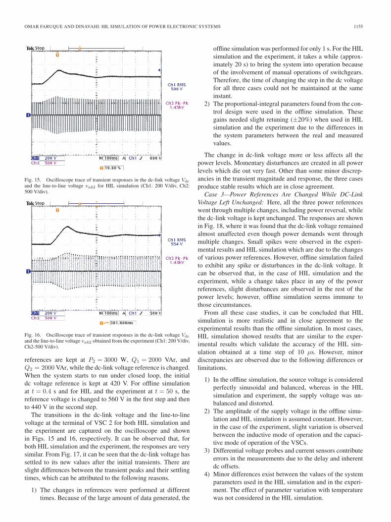
Fig. 15. Oscilloscope trace of transient responses in the dc-link voltage Vdc

and the line-to-line voltage vab2 for HIL simulation (Ch1: 200 V/div, Ch2:500 V/div).

Fig. 16. Oscilloscope trace of transient responses in the dc-link voltage Vdc

and the line-to-line voltage vab2 obtained from the experiment (Ch1: 200 V/div,Ch2-500 V/div).

references are kept at P2 = 3000 W, Q1 = 2000 VAr, andQ2 = 2000 VAr, while the dc-link voltage reference is changed.When the system starts to run under closed loop, the initialdc voltage reference is kept at 420 V. For offline simulationat t = 0.4 s and for HIL and the experiment at t = 50 s, thereference voltage is changed to 560 V in the first step and thento 440 V in the second step.

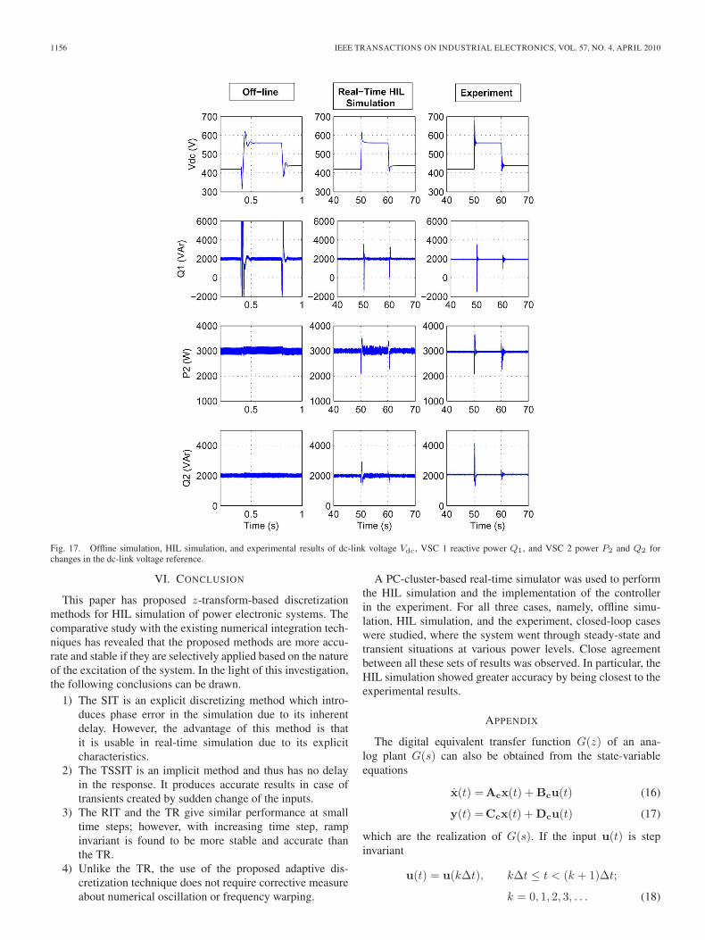
The transitions in the dc-link voltage and the line-to-linevoltage at the terminal of VSC 2 for both HIL simulation andthe experiment are captured on the oscilloscope and shownin Figs. 15 and 16, respectively. It can be observed that, forboth HIL simulation and the experiment, the responses are verysimilar. From Fig. 17, it can be seen that the dc-link voltage hassettled to its new values after the initial transients. There areslight differences between the transient peaks and their settlingtimes, which can be attributed to the following reasons.

1) The changes in references were performed at differenttimes. Because of the large amount of data generated, the

offline simulation was performed for only 1 s. For the HILsimulation and the experiment, it takes a while (approx-imately 20 s) to bring the system into operation becauseof the involvement of manual operations of switchgears.Therefore, the time of changing the step in the dc voltagefor all three cases could not be maintained at the sameinstant.

2) The proportional-integral parameters found from the con-trol design were used in the offline simulation. Thesegains needed slight retuning (±20%) when used in HILsimulation and the experiment due to the differences inthe system parameters between the real and measuredvalues.

The change in dc-link voltage more or less affects all thepower levels. Momentary disturbances are created in all powerlevels which die out very fast. Other than some minor discrep-ancies in the transient magnitude and response, the three casesproduce stable results which are in close agreement.

Case 3—Power References Are Changed While DC-LinkVoltage Left Unchanged: Here, all the three power referenceswent through multiple changes, including power reversal, whilethe dc-link voltage is kept unchanged. The responses are shownin Fig. 18, where it was found that the dc-link voltage remainedalmost unaffected even though power demands went throughmultiple changes. Small spikes were observed in the experi-mental results and HIL simulation which are due to the changesof various power references. However, offline simulation failedto exhibit any spike or disturbances in the dc-link voltage. Itcan be observed that, in the case of HIL simulation and theexperiment, while a change takes place in any of the powerreferences, slight disturbances are observed in the rest of thepower levels; however, offline simulation seems immune tothose circumstances.

From all these case studies, it can be concluded that HILsimulation is more realistic and in close agreement to theexperimental results than the offline simulation. In most cases,HIL simulation showed results that are similar to the exper-imental results which validate the accuracy of the HIL sim-ulation obtained at a time step of 10 μs. However, minordiscrepancies are observed due to the following differences orlimitations.

1) In the offline simulation, the source voltage is consideredperfectly sinusoidal and balanced, whereas in the HILsimulation and experiment, the supply voltage was un-balanced and distorted.

2) The amplitude of the supply voltage in the offline simu-lation and HIL simulation is assumed constant. However,in the case of the experiment, slight variation is observedbetween the inductive mode of operation and the capaci-tive mode of operation of the VSCs.

3) Differential voltage probes and current sensors contributeerrors in the measurements due to the delay and inherentdc offsets.

4) Minor differences exist between the values of the systemparameters used in the HIL simulation and in the experi-ment. The effect of parameter variation with temperaturewas not considered in the HIL simulation.


Fig. 17. Offline simulation, HIL simulation, and experimental results of dc-link voltage Vdc, VSC 1 reactive power Q1, and VSC 2 power P2 and Q2 forchanges in the dc-link voltage reference.

VI. CONCLUSION

This paper has proposed z-transform-based discretizationmethods for HIL simulation of power electronic systems. Thecomparative study with the existing numerical integration tech-niques has revealed that the proposed methods are more accu-rate and stable if they are selectively applied based on the natureof the excitation of the system. In the light of this investigation,the following conclusions can be drawn.

1) The SIT is an explicit discretizing method which intro-duces phase error in the simulation due to its inherentdelay. However, the advantage of this method is thatit is usable in real-time simulation due to its explicitcharacteristics.

2) The TSSIT is an implicit method and thus has no delayin the response. It produces accurate results in case oftransients created by sudden change of the inputs.

3) The RIT and the TR give similar performance at smalltime steps; however, with increasing time step, rampinvariant is found to be more stable and accurate thanthe TR.

4) Unlike the TR, the use of the proposed adaptive dis-cretization technique does not require corrective measureabout numerical oscillation or frequency warping.

A PC-cluster-based real-time simulator was used to performthe HIL simulation and the implementation of the controllerin the experiment. For all three cases, namely, offline simu-lation, HIL simulation, and the experiment, closed-loop caseswere studied, where the system went through steady-state andtransient situations at various power levels. Close agreementbetween all these sets of results was observed. In particular, theHIL simulation showed greater accuracy by being closest to theexperimental results.

APPENDIX

The digital equivalent transfer function G(z) of an ana-log plant G(s) can also be obtained from the state-variableequations

x(t) =Acx(t) + Bcu(t) (16)

y(t) =Ccx(t) + Dcu(t) (17)

which are the realization of G(s). If the input u(t) is stepinvariant

u(t) = u(kΔt), kΔt ≤ t < (k + 1)Δt;

k = 0, 1, 2, 3, . . . (18)


Fig. 18. Offline simulation, HIL simulation, and experimental result of dc-link voltage Vdc, VSC 1 reactive power Q1, and VSC 2 power P2 and Q2 whenpower references were changed.

then the output y(t) at t = kΔt can be described as

x(k + 1)Δt =Adx(kΔt) + Bdu(kΔt) (19)

y(kΔt) =Cdx(kΔt) + Ddu(kΔt) (20)

where Ad = eAcΔt, Bd = (∫ Δt

0 eAcτdτ)Bc = [eAcΔt −1]A−1

c Bc, Cc = Cd, and Dc = Dd.For TSSIT, the equations are

x(k + 1)Δt =Adx(kΔt) + Bdu(k + 1)Δt (21)

y(kΔt) =Cdx(kΔt) + Ddu(kΔt). (22)

For a ramp-invariant input

u(t)=u(kΔt)+u [(k+1)Δt]−u(kΔt)

Δt× (t−kΔt) (23)

where kΔt ≤ t ≤ (k + 1)Δt, k = 0, 1, 2, 3, . . ., and the outputy(t) at t = kΔt can be described as [19]

x(k + 1)Δt =Fdx(kΔt) + Gdu(kΔt) + Hdu(k + 1)Δt

y(kΔt) =Cdx(kΔt) + Ddu(kΔt) (24)

where

Fd = eAcΔt =∞∑

n=0

1n!

(AcΔt)n (25)

Gd =[eAcΔt(−1 + AcΔt) + 1

] (A2

cΔt2)−1 BcΔt

=∞∑

n=0

1n(n + 2)!

(AcΔt)n × BcΔt (26)

Hd =[eAcΔt − 1 − AcΔt

] (A2

cΔt2)−1 BcΔt

=∞∑

n=0

1(n + 2)!

(AcΔt)n × BcΔt (27)

Cd =Cc (28)Dd =Dc. (29)

REFERENCES

[1] H. Li, M. Steurer, S. Woodruff, L. Shi, and D. Zhang, “Developmentof a unified design, test, and research platform for wind energy systemsbased on hardware-in-the-loop real-time simulation,” IEEE Trans. Ind.Electron., vol. 53, no. 4, pp. 1144–1151, Jun. 2006.

[2] A. Bouscayrol, X. Guillaud, R. Teodorescu, P. Delarue, and W. Lhomme,“Energetic macroscopic representation and inversion-based control illus-trated on a wind-energy-conversion system using hardware-in-the-loopsimulation,” IEEE Trans. Ind. Electron., vol. 56, no. 12, pp. 4826–4835,Dec. 2009.


[3] B. Lu, X. Wu, H. Figueroa, and A. Monti, “A low-cost real-time hardware-in-the-loop testing approach of power electronics control,” IEEE Trans.Ind. Electron., vol. 54, no. 2, pp. 919–931, Apr. 2007.

[4] G. G. Parma and V. Dinavahi, “Real-time digital hardware simulation ofpower electronics and drives,” IEEE Trans. Power Del., vol. 22, no. 2,pp. 1235–1246, Apr. 2007.

[5] T. Zhou, B. Francois, M. Hadi Lebbal, and S. Lecoeuche, “Real-timeemulation of a hydrogen-production process for assessment of an activewind-energy conversion system,” IEEE Trans. Ind. Electron., vol. 56,no. 3, pp. 737–746, Mar. 2009.

[6] D. Hercog, B. Gergic, S. Uran, and K. Jezernik, “A DSP-based remotecontrol laboratory,” IEEE Trans. Ind. Electron., vol. 54, no. 6, pp. 3057–3068, Dec. 2007.

[7] A. Bouscayrol, “Different types of hardware-in-the-loop simulation forelectric drives,” in Proc. IEEE ISIE, Cambridge, U.K., Jun. 2008,pp. 2146–2151.

[8] T. L. Maguire and A. M. Gole, “Digital simulation of flexible topologypower electronic apparatus in power systems,” IEEE Trans. Power Del.,vol. 6, no. 4, pp. 1831–1840, Oct. 1991.

[9] V. R. Dinavahi, M. R. Iravani, and R. Bonert, “Real-time digital simulationof power electronic apparatus interfaced with digital controllers,” IEEETrans. Power Del., vol. 16, no. 4, pp. 775–781, Oct. 2001.

[10] B. D. Kelper, L. A. Dessaint, K. A. Haddad, and H. Nakra, “A comprehen-sive approach to fixed-step simulation of switched circuits,” IEEE Trans.Power Electron., vol. 17, no. 2, pp. 216–224, Mar. 2002.

[11] V. Dinavahi, R. Iravani, and R. Bonert, “Design of a real-time digitalsimulator for a D-STATCOM system,” IEEE Trans. Ind. Electron., vol. 51,no. 5, pp. 1001–1008, Oct. 2004.

[12] K. Strunz, L. R. Linares, J. R. Marti, O. Huet, and X. Lombard, “Efficientand accurate representation of asynchronous network structure changingphenomena in digital real time simulators,” IEEE Trans. Power Syst.,vol. 15, no. 2, pp. 586–592, May 2000.

[13] M. O. Faruque, V. Dinavahi, and W. Xu, “Algorithms for the account-ing of multiple switching events in digital simulation of power elec-tronic systems,” IEEE Trans. Power Del., vol. 20, no. 2, pp. 1157–1167,Apr. 2005.

[14] H. W. Dommel, “Digital computer solution of electromagnetic transientsin single and multi-phase networks,” IEEE Trans. Power App. Syst.,vol. PAS-88, no. 4, pp. 388–395, Apr. 1969.

[15] J. R. Marti and J. Lin, “Suppression of numerical oscillations in theEMTP,” IEEE Trans. Power Syst., vol. 4, no. 2, pp. 739–747, May 1989.

[16] N. R. Watson and J. Arrillaga, Power Systems Electromagnetic TransientsSimulation. Stevenage, U.K.: IET, 2003.

[17] L. Naredo, A. Ramirez, A. Ametani, A. Gutierrez, A. Mansoldo, A. Gole,A. Lima, A. Morched, B. Gustavsen, D. Wilcox, F. Uribe, F. Moreira,F. de Leon, J. Martinez, L. Guardado, M. Davila, M. Ritual, N. Nagaoka,N. Watson, P. Gomez, P. Moreno, R. Iravani, S. Carneiro, T. Noda,V. Dinavahi, V. Ortiz, and W. Neves, “z-transform-based methods forelectromagnetic transient simulation,” IEEE Trans. Power Del., vol. 22,no. 3, pp. 1799–1805, Jul. 2007.

[18] C.-T. Chen, Analog and Digital Control System Design: Transfer-Function, State-Space, and Algebraic Methods. Philadelphia, PA:Saunders, 1993.

[19] L. O. Chua and P. M. Lin, Computer Aided Analysis of Electronic Circuits:Algorithms and Computational Techniques. Englewood Cliffs, NJ:Prentice-Hall, 1975.

[20] L.-F. Pak, M. O. Faruque, X. Nie, and V. Dinavahi, “A versatile cluster-based real-time digital simulator for power engineering research,” IEEETrans. Power Syst., vol. 21, no. 2, pp. 455–465, May 2006.

[21] RT-LAB Manual, OPAL-RT Technol. Inc., Montreal, QC, Canada, 2008.[22] C. Schauder and H. Mehta, “Vector analysis and control of advanced

static VAR compensators,” Proc. Inst. Elect. Eng., vol. 140, pt. C, no. 4,pp. 299–306, Jul. 1993.

M. Omar Faruque (SM’03–M’08) received theB.Sc.Engg. degree from Chittagong Universityof Engineering and Technology, Chittagong,Bangladesh, in 1992, the M.Engg.Sc. degree fromthe University of Malaya, Kuala Lumpur, Malaysia,in 1999, and the Ph.D. degree from the University ofAlberta, Edmonton, AB, Canada, in 2008.

He is currently an Assistant Scholar/Scientistin The Center for Advanced Power Systems, TheFlorida State University, Tallahassee. His researchinterests are in the areas of hardware-in-the-loop

simulation, modeling, and simulation of flexible ac transmission systems,HVDC, renewable resources, and grid connection of distributed resources andtheir impacts.

Venkata Dinavahi (S’94–M’00–SM’08) receivedthe B.Eng. degree in electrical engineering fromVisvesvaraya Regional College of Engineering,Nagpur, India, in 1993, the M.Tech. degree fromthe Indian Institute of Technology, Kanpur, India, in1996, and the Ph.D. degree in electrical and com-puter engineering from the University of Toronto,Toronto, ON, Canada, in 2000.

He is currently an Associate Professor at theUniversity of Alberta, Edmonton, AB, Canada. Hisresearch interests include real-time simulation of

power systems and power electronic systems, large-scale system simulation,and parallel and distributed computing.

hardware-in-the-loop simulation of power electronic...

Documents