hardware -in the loop simulation for a small unmanned ... · vehicle (uav) are presented. the...
TRANSCRIPT
Paper: ASAT-16-077-GU
16th
International Conference on
AEROSPACE SCIENCES & AVIATION TECHNOLOGY,
ASAT - 16 – May 26 - 28, 2015, E-Mail: [email protected]
Military Technical College, Kobry Elkobbah, Cairo, Egypt
Tel : +(202) 24025292 – 24036138, Fax: +(202) 22621908
Hardware-in-the-Loop Simulation for a
Small Unmanned Aerial Vehicle A. Shawky
*, A. Bayoumy Aly
†, A. Nashar
‡, and M. Elsayed
§
Abstract: Modeling, guidance and control experimental results for a small unmanned aerial
vehicle (UAV) are presented. The numerical values of the aerodynamic derivatives are
computed via the Digital DATCOM software using the geometric parameters of the airplane.
A hardware-in-the-loop (HIL) simulation environment is developed to support and validate
the small UAV model autopilot hardware and software development. The HIL simulation
incorporates a high-fidelity dynamic model that includes the sensor and actuator models, the
test bed HIL system used to facilitate the development of the flight control system (FCS).
Furthermore, design of the guidance laws, autopilot implementation on the embedded system
are integrated with the HIL simulation. A mission has been design in order to validate the
guidance and control loops. Finally, a user friendly graphical interface that incorporates
external stick commands and 3-D visualization of the vehicle’s motion completes the
simulation environment.
Keywords: UAV Modeling, UAV guidance and control, Simulation, X-plane.
1. Introduction In the past decade Unmanned Aerial Vehicles (UAVs) have rapidly grown into a major field
of robotics in both industry and academia. Many well established platforms have been
developed, and the demand continues to grow. However, the Unmanned Aerial Vehicles
(UAV's) have gained increasing due to their low cost and improved autonomy. UAV's have
been employed in numerous applications, civilian as well as military. For certain missions,
UAV’s have needed to integrate both hardware and software in a seamless manner.
Applications include surveillance, object tracking, and crop dusting. A successful certification
of a new autopilot can only be enabled by extensive flight testing to debug both the hardware
and the software before deploying the UAV in the field. Despite the necessity of real flight
tests, simulation-based testing also plays a very important role. It can save time and effort
prior to conducting actual flight tests. In particular, hardware in-the-loop (HIL) simulation
testing should be adopted whenever possible to validate together both the hardware and the
software under realistic conditions.
Building a simulation model starts with setting up the equations of motion for a 6-DOF
dynamic model [1,5,6]. Traditionally, the dimensionless coefficients for the aerodynamic
forces and moments are approximated by a linear sum of contributing parameters utilizing the
stability and control derivatives in a specified flight condition. Precise knowledge of such
derivatives is essential towards the development of a high fidelity simulation. Many recent
publications have addressed such a problem (e.g. [11]).
* R&D of Egyptian Air force, Egypt, [email protected]
† R&D of Egyptian Air force, Egypt, [email protected] ‡ R&D of Egyptian Air force, Egypt, [email protected]
§ R&D of Egyptian Air force, Egypt, [email protected]
Paper: ASAT-16-077-GU
This paper focuses on the design and building of a fully functional UAV test bed platform.
The test-bed will include an enhanced Hardware-In-the-Loop simulation "HIL" system
designed to facilitate the development of the Flight Control System (FCS) and the guidance
and navigation system and how to visualize that model in a Flight Simulator with the ability
to perform autonomous flight simulation [2,3,4].
The paper is organized as follow: Section 2 explains the dynamical model and the nonlinear
mathematical equations and dynamical modeling and system identifications. The controller
design and simulation are presented in Section 3. Section 4 covers the hardware in the loop
simulation (HIL) as well as the real-time trajectory tracking is presented. Finally, conclusions
are addressed in Section 5.
2. Nonlinear Model and Dynamics Equations
Standard 6-DOF equations of motion for a conventional aircraft are used for modeling and
simulation of a small UAV model [5,6]. Flat Earth approximation provides a reasonable
modeling assumption when the vehicle operates over a small area. The body-axes force,
moments, kinematics and navigations equations are as follows:
Force equations:
(1-a)
(1-b)
(1-c)
Moment equations:
(2-a)
(2-b)
(2-c)
Kinematic equations:
(3-a)
(3-b)
(3-c)
Navigation equations:
(4-a)
(4-b)
(4-c)
The equation are in terms of the body frame translation velocity vector components (U,V,W),
body frame angular velocity vector components (p,q,r), Euler angles ( ), gravity (g),
mass (m), external forces ( ), Rolling Moment ( ), pitching moment (M), yawing
moment (N), and the resulting body frame linear and angular accelerations ( ) and
( , , ) [5]. The aerodynamic forces and moments are obtained from the dimensionless
aerodynamic coefficients at a given flight condition as follows,
, , (5-a) , , (5-b)
Where dynamic pressure, S wing reference area, b wing span, wing mean geometric
chord, and ( ) aerodynamic forces and moments in terms of dimensionless
coefficients. The nonlinear aircraft model is linearized about several trim conditions; the state
space linear model of the aircraft is derived using the already available stability derivatives
found in section 2.1. The linearized state space model is needed to develop the guidance and
control laws [7,9]. It is used to develop airspeed hold, altitude hold, and attitude hold as well
as for ground and navigation control. The longitudinal and lateral models are derived.
Paper: ASAT-16-077-GU
2.1 Longitudinal Model
The following state space model is the linear longitudinal model for the Cessna 182 ¼ scale
RC model linearized around a typical flight condition
(6)
Where the state variables , refer to the longitudinal velocities, and , the pitch
rate, and the angle of inclination . In addition to the above states, the altitude is added to
account for the height above the ground. The control input , is the elevator deflection
angle , and the engine throttle lever .
2.2 Lateral Model
Similar to the longitudinal model, the dynamics describing lateral perturbations about the
same equilibrium trim conditions previously mentioned is written below in concise state space
form.
(7)
Where is the sideslip angle, and represent the roll and yaw rates and is the roll angle.
The aileron control input is denoted by , and the rudder control input .
3. Navigation and Guidance Control Laws Controller is developed for the testing autopilot. The current controller consists of two main
parts, a Mission waypoint generator, and a trajectory generator. The controller has not been
optimized due to the scope of this paper research.
3.1 Guidance Design The first part of the controller is the waypoint generator (WG). The WG simply updates the
current waypoint to the next waypoint to be achieved. The entire waypoint set is generated by
the UAV user and stored in a list (WL). Once a waypoint has been reached, the WG updates
the list and the UAV is steered to the next waypoint. It should be noted that the waypoint
does not have to be reached explicitly, but rather a sphere has been developed around the
waypoints center in which if the UAV reaches the “tolerance” sphere, the waypoint is
considered reached and the WG updates to the next waypoint which known as waypoint
tracking [2,7].
The second part of the controller is to generate desired trajectories for the UAV to track in
terms of UAV heading and UAV altitude . The UAV trajectories are generated
based on a desired set of coordinates to be reached by the UAV, , where
are the desired latitude, longitude, and altitude respectively. Once the
UAV reaches the current coordinate vector within the tolerance sphere, the vector is
updated and a new reference trajectory is generated.
Paper: ASAT-16-077-GU
The trajectories of the navigation controller are generated based on the current UAV position
and the desired UAV position. The first signal generated is the altitude trajectory in which the
altitude error is computed as , from this error a desired altitude trajectory is
generated as
(8)
Where is defined as a function of the error in altitude.
The second signal generated by the navigation controller is the desired heading trajectory in
which the heading error is calculated based on the current UAV position, the desired UAV
position, and the current UAV heading. Error calculation in altitude is done by simply
subtracting two values, but error calculation in the latitude/longitude plane is much more
complex. Several methods are tested, but only one worked reliably with very little
computational load [10].
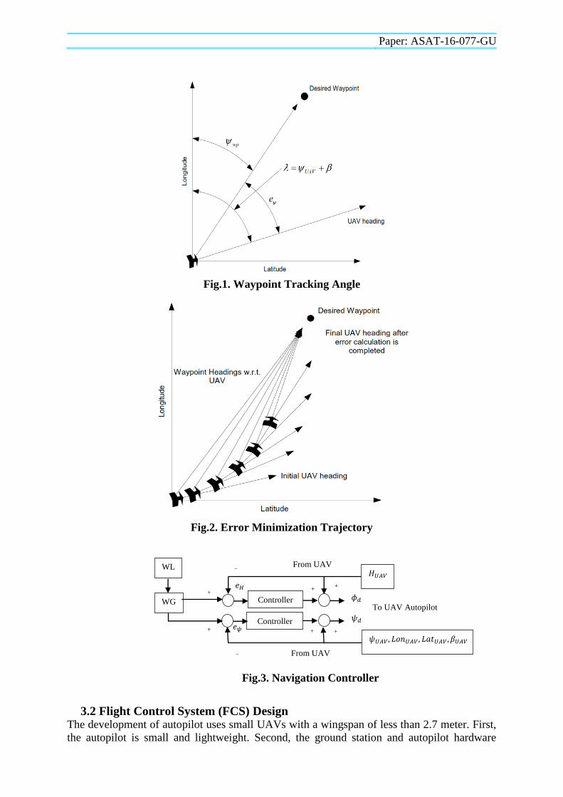
This method developed for error calculation in the latitude/longitude plane uses a
triangulation method. The advantage of the triangulation method is that the computational
load is negligible. The method consists of subtracting two vector values, and computing an
inverse tangent of the result. The error is calculated as
(9)
Where:
, and (10)
In Eq. 10, is the waypoint heading with respect to the UAV position updated
continuously as the UAV travels in the latitude/longitude plane, and and are defined as
(11)
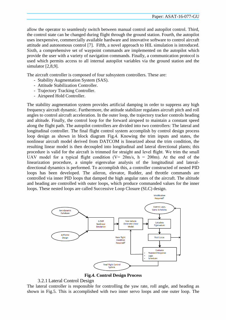
In Eq. 10, the actual UAV heading is calculated as the current UAV heading with the
addition of any UAV sideslip [10]. A graphical representation of Eqs. 9 to 11 is shown in
Fig.1, with a sample error minimization trajectory in Fig.2.
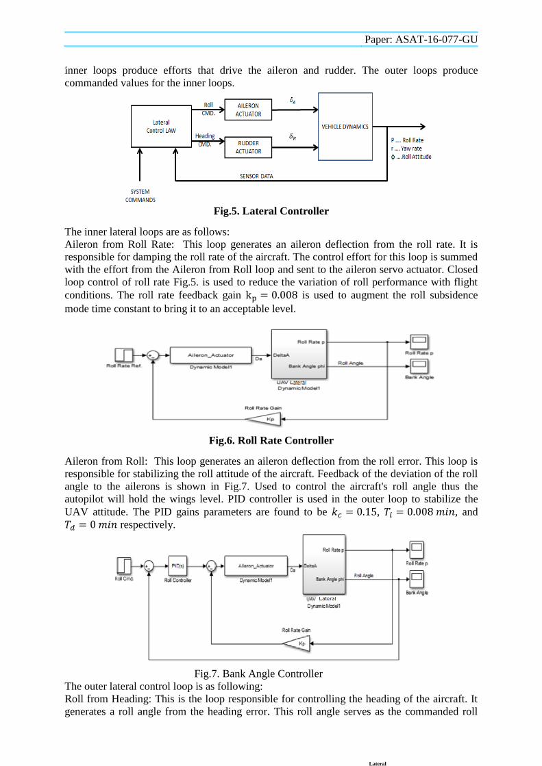
From Eq. 9, the new heading trajectory can be generated as
(12)
Where is defined as a function of heading error. The complete navigation portion of
the controller can be seen in Fig.3. The blocks labeled controller are defined as the control
system and are discussed in detail in this section [10].
Paper: ASAT-16-077-GU
Fig.1. Waypoint Tracking Angle
Fig.2. Error Minimization Trajectory
3.2 Flight Control System (FCS) Design The development of autopilot uses small UAVs with a wingspan of less than 2.7 meter. First,
the autopilot is small and lightweight. Second, the ground station and autopilot hardware
WG
WL
Controller
Controller
From UAV
From UAV
To UAV Autopilot
Fig.3. Navigation Controller
Paper: ASAT-16-077-GU
allow the operator to seamlessly switch between manual control and autopilot control. Third,
the control state can be changed during flight through the ground station. Fourth, the autopilot
uses inexpensive, commercially available hardware and innovative software to control aircraft
attitude and autonomous control [7]. Fifth, a novel approach to HIL simulation is introduced.
Sixth, a comprehensive set of waypoint commands are implemented on the autopilot which
provide the user with a variety of navigation commands. Finally, a communication protocol is
used which permits access to all internal autopilot variables via the ground station and the
simulator [2,8,9].
The aircraft controller is composed of four subsystem controllers. These are:
- Stability Augmentation System (SAS).
- Attitude Stabilization Controller.
- Trajectory Tracking Controller.
- Airspeed Hold Controller.
The stability augmentation system provides artificial damping in order to suppress any high
frequency aircraft dynamic. Furthermore, the attitude stabilizer regulates aircraft pitch and roll
angles to control aircraft acceleration. In the outer loop, the trajectory tracker controls heading
and altitude. Finally, the control loop for the forward airspeed to maintain a constant speed
along the flight path. The autopilot controllers are divided into two controllers: The lateral and
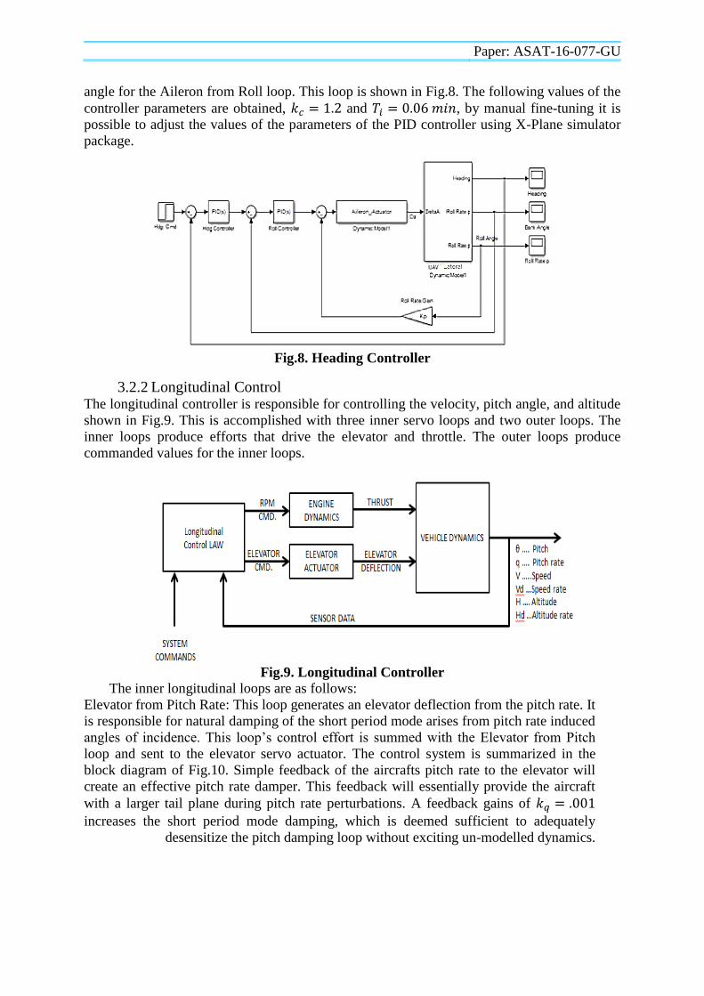
longitudinal controller. The final flight control system accomplish by control design process
loop design as shown in block diagram Fig.4. Knowing the trim inputs and states, the
nonlinear aircraft model derived from DATCOM is linearized about the trim condition, the
resulting linear model is then decoupled into longitudinal and lateral directional plants; this
procedure is valid for the aircraft is trimmed for straight and level flight. We trim the small
UAV model for a typical flight condition (V= 20m/s, h = 200m). At the end of the
linearization procedure, a simple eigenvalue analysis of the longitudinal and lateral-
directional dynamics is performed. To accomplish this, a controller constructed of nested PID
loops has been developed. The aileron, elevator, Rudder, and throttle commands are
controlled via inner PID loops that damped the high angular rates of the aircraft. The altitude
and heading are controlled with outer loops, which produce commanded values for the inner
loops. These nested loops are called Successive Loop Closure (SLC) design.
Fig.4. Control Design Process
3.2.1 Lateral Control Design The lateral controller is responsible for controlling the yaw rate, roll angle, and heading as
shown in Fig.5. This is accomplished with two inner servo loops and one outer loop. The
Paper: ASAT-16-077-GU
inner loops produce efforts that drive the aileron and rudder. The outer loops produce
commanded values for the inner loops.
Fig.5. Lateral Controller
The inner lateral loops are as follows:
Aileron from Roll Rate: This loop generates an aileron deflection from the roll rate. It is
responsible for damping the roll rate of the aircraft. The control effort for this loop is summed
with the effort from the Aileron from Roll loop and sent to the aileron servo actuator. Closed
loop control of roll rate Fig.5. is used to reduce the variation of roll performance with flight
conditions. The roll rate feedback gain is used to augment the roll subsidence
mode time constant to bring it to an acceptable level.
Fig.6. Roll Rate Controller
Aileron from Roll: This loop generates an aileron deflection from the roll error. This loop is
responsible for stabilizing the roll attitude of the aircraft. Feedback of the deviation of the roll
angle to the ailerons is shown in Fig.7. Used to control the aircraft's roll angle thus the
autopilot will hold the wings level. PID controller is used in the outer loop to stabilize the
UAV attitude. The PID gains parameters are found to be , , and
respectively.
Fig.7. Bank Angle Controller
The outer lateral control loop is as following:
Roll from Heading: This is the loop responsible for controlling the heading of the aircraft. It
generates a roll angle from the heading error. This roll angle serves as the commanded roll
Lateral
Paper: ASAT-16-077-GU
angle for the Aileron from Roll loop. This loop is shown in Fig.8. The following values of the
controller parameters are obtained, and , by manual fine-tuning it is
possible to adjust the values of the parameters of the PID controller using X-Plane simulator
package.
Fig.8. Heading Controller
3.2.2 Longitudinal Control The longitudinal controller is responsible for controlling the velocity, pitch angle, and altitude
shown in Fig.9. This is accomplished with three inner servo loops and two outer loops. The
inner loops produce efforts that drive the elevator and throttle. The outer loops produce
commanded values for the inner loops.
Fig.9. Longitudinal Controller
The inner longitudinal loops are as follows:
Elevator from Pitch Rate: This loop generates an elevator deflection from the pitch rate. It
is responsible for natural damping of the short period mode arises from pitch rate induced
angles of incidence. This loop’s control effort is summed with the Elevator from Pitch
loop and sent to the elevator servo actuator. The control system is summarized in the
block diagram of Fig.10. Simple feedback of the aircrafts pitch rate to the elevator will
create an effective pitch rate damper. This feedback will essentially provide the aircraft
with a larger tail plane during pitch rate perturbations. A feedback gains of
increases the short period mode damping, which is deemed sufficient to adequately
desensitize the pitch damping loop without exciting un-modelled dynamics.
Paper: ASAT-16-077-GU
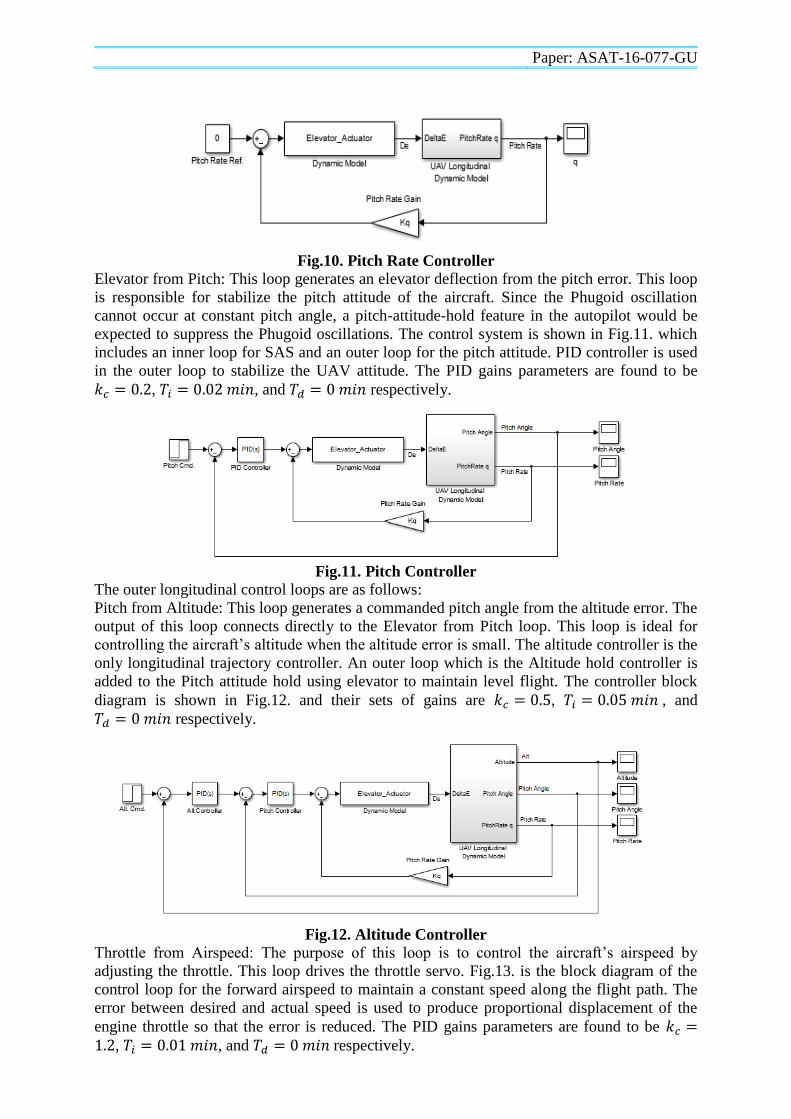
Fig.10. Pitch Rate Controller
Elevator from Pitch: This loop generates an elevator deflection from the pitch error. This loop
is responsible for stabilize the pitch attitude of the aircraft. Since the Phugoid oscillation
cannot occur at constant pitch angle, a pitch-attitude-hold feature in the autopilot would be
expected to suppress the Phugoid oscillations. The control system is shown in Fig.11. which
includes an inner loop for SAS and an outer loop for the pitch attitude. PID controller is used
in the outer loop to stabilize the UAV attitude. The PID gains parameters are found to be
, , and respectively.
Fig.11. Pitch Controller
The outer longitudinal control loops are as follows:
Pitch from Altitude: This loop generates a commanded pitch angle from the altitude error. The
output of this loop connects directly to the Elevator from Pitch loop. This loop is ideal for
controlling the aircraft’s altitude when the altitude error is small. The altitude controller is the
only longitudinal trajectory controller. An outer loop which is the Altitude hold controller is
added to the Pitch attitude hold using elevator to maintain level flight. The controller block
diagram is shown in Fig.12. and their sets of gains are , , and
respectively.
Fig.12. Altitude Controller
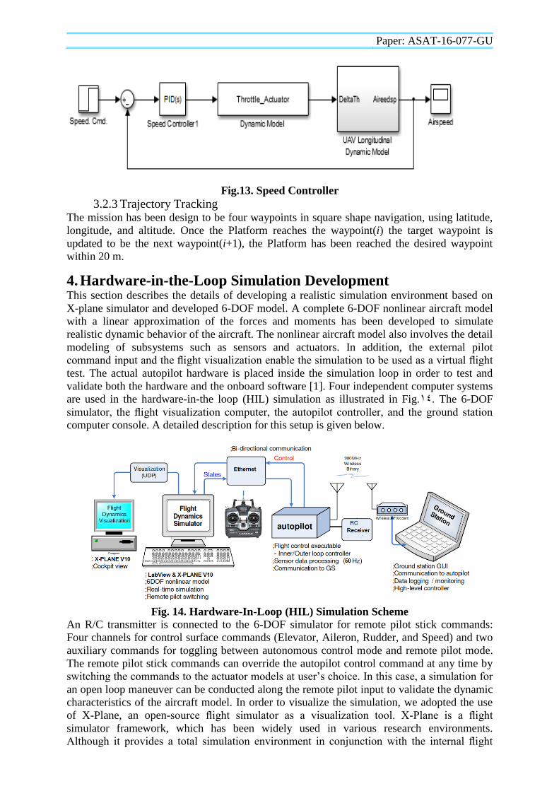
Throttle from Airspeed: The purpose of this loop is to control the aircraft’s airspeed by
adjusting the throttle. This loop drives the throttle servo. Fig.13. is the block diagram of the
control loop for the forward airspeed to maintain a constant speed along the flight path. The
error between desired and actual speed is used to produce proportional displacement of the
engine throttle so that the error is reduced. The PID gains parameters are found to be , , and respectively.
Paper: ASAT-16-077-GU
Fig.13. Speed Controller
3.2.3 Trajectory Tracking The mission has been design to be four waypoints in square shape navigation, using latitude,
longitude, and altitude. Once the Platform reaches the waypoint(i) the target waypoint is
updated to be the next waypoint(i+1), the Platform has been reached the desired waypoint
within 20 m.
4. Hardware-in-the-Loop Simulation Development This section describes the details of developing a realistic simulation environment based on
X-plane simulator and developed 6-DOF model. A complete 6-DOF nonlinear aircraft model
with a linear approximation of the forces and moments has been developed to simulate
realistic dynamic behavior of the aircraft. The nonlinear aircraft model also involves the detail
modeling of subsystems such as sensors and actuators. In addition, the external pilot
command input and the flight visualization enable the simulation to be used as a virtual flight
test. The actual autopilot hardware is placed inside the simulation loop in order to test and
validate both the hardware and the onboard software [1]. Four independent computer systems
are used in the hardware-in-the loop (HIL) simulation as illustrated in Fig.41. The 6-DOF
simulator, the flight visualization computer, the autopilot controller, and the ground station
computer console. A detailed description for this setup is given below.
Fig. 14. Hardware-In-Loop (HIL) Simulation Scheme
An R/C transmitter is connected to the 6-DOF simulator for remote pilot stick commands:
Four channels for control surface commands (Elevator, Aileron, Rudder, and Speed) and two
auxiliary commands for toggling between autonomous control mode and remote pilot mode.
The remote pilot stick commands can override the autopilot control command at any time by
switching the commands to the actuator models at user’s choice. In this case, a simulation for
an open loop maneuver can be conducted along the remote pilot input to validate the dynamic
characteristics of the aircraft model. In order to visualize the simulation, we adopted the use
of X-Plane, an open-source flight simulator as a visualization tool. X-Plane is a flight
simulator framework, which has been widely used in various research environments.
Although it provides a total simulation environment in conjunction with the internal flight
Paper: ASAT-16-077-GU
dynamics models, we used X-Plane as a visualization tool combined with our developed 6-
DOF simulator. By doing this, X-Plane receives the simulated states from the simulator at a
fixed update rate 20 Hz to constantly refresh the virtual scenes that have been generated along
the user’s convenient view angles. The ability to record the pilot stick command with
visualization via X-Plane allows the simulation environment to replace a real experiment to
save time and effort. The open loop behavior of the UAV can be tested and validated by a
remote pilot via R/C transmitter input device, and the closed loop control performance can be
verified and demonstrated by conducting virtual experiments in advance to a real flight test.
The 6-DOF simulator X-Plane exchanges sensor and control command signals with the
autopilot via a User Datagram Protocol (UDP) network protocol established between the
simulator and autopilot. The sensor output data include different sensor outputs from INS,
GPS, magnetometers, etc., and are packed into a binary packet. This binary packet begins
with a designated header to distinguish between different packets and ends by a trailer for data
consistency check. The UDP communication is configured for a baud rate of 115200 bps,
which allows communicating by transmitting the sensor packet at 20 Hz. The control
command data from the autopilot are composed of four PWM commands for each actuator,
resulting in a binary packet of 11 bytes in length associated with header and trailer to be
transmitted at a 20 Hz update rate. The HIL Bridge shown in Fig.14 is then incorporated into
the 6-DOF Simulink model to handle the bidirectional communication.
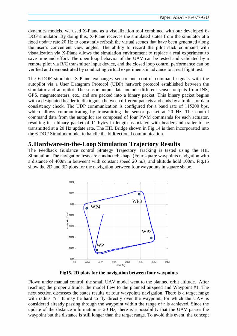
5. Hardware-in-the-Loop Simulation Trajectory Results The Feedback Guidance control Strategy Trajectory Tracking is tested using the HIL
Simulation. The navigation tests are conducted; shape (Four square waypoints navigation with
a distance of 400m in between) with constant speed 20 m/s, and altitude hold 100m. Fig.15
show the 2D and 3D plots for the navigation between four waypoints in square shape.
Fig15. 2D plots for the navigation between four waypoints
Flown under manual control, the small UAV model went to the planned orbit altitude. After
reaching the proper altitude, the model flew to the planned airspeed and Waypoint #1. The
next section discusses the states results of four waypoints navigation. There is a target range
with radius “r”. It may be hard to fly directly over the waypoint, for which the UAV is
considered already passing through the waypoint within the range of r is achieved. Since the
update of the distance information is 20 Hz, there is a possibility that the UAV passes the
waypoint but the distance is still longer than the target range. To avoid this event, the concept
29.8 29.802 29.804 29.806 29.808 29.81 29.812 29.81430.82
30.822
30.824
30.826
30.828
30.83
30.832
30.834
Latitude [Deg]
Longitude [D
eg]
WP4
WP3
WP
1
WP2
Paper: ASAT-16-077-GU
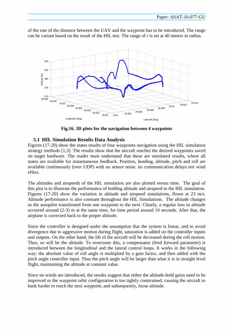
of the rate of the distance between the UAV and the waypoint has to be introduced. The range
can be variant based on the result of the HIL test. The range of r is set at 40 meters in radius.
Fig.16. 3D plots for the navigation between 4 waypoints
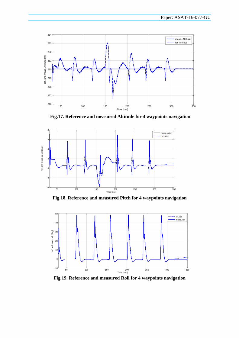
5.1 HIL Simulation Results Data Analysis Figures (17-20) show the states results of four waypoints navigation using the HIL simulation
strategy methods [1,3]. The results show that the aircraft reaches the desired waypoints saved
on target hardware. The reader must understand that these are simulated results, where all
states are available for instantaneous feedback. Position, heading, altitude, pitch and roll are
available continuously (over UDP) with no sensor noise, no communication delays nor wind
effect.
The altitudes and airspeeds of the HIL simulation are also plotted versus time. The goal of
this plot is to illustrate the performance of holding altitude and airspeed in the HIL simulation.
Figures (17-20) show the variation in altitude and airspeed simulations, flown at 23 m/s.
Altitude performance is also constant throughout the HIL Simulations. The altitude changes
as the autopilot transitioned from one waypoint to the next. Clearly, a regular loss in altitude
occurred around (2-3) m at the same time, for time period around 10 seconds. After that, the
airplane is corrected back to the proper altitude.
Since the controller is designed under the assumption that the system is linear, and to avoid
divergence due to aggressive motion during flight, saturation is added on the controller inputs
and outputs. On the other hand, the lift of the aircraft will be decreased during the roll motion.
Thus, so will be the altitude. To overcome this, a compensator (feed forward parameter) is
introduced between the longitudinal and the lateral control loops. It works in the following
way: the absolute value of roll angle is multiplied by a gain factor, and then added with the
pitch angle controller input. Thus the pitch angle will be larger than what it is in straight level
flight, maintaining the altitude at constant value.
Since no winds are introduced, the results suggest that either the altitude-hold gains need to be
improved or the waypoint orbit configuration is too tightly constrained, causing the aircraft to
bank harder to reach the next waypoint, and subsequently, loose altitude.
29.829.802
29.80429.806
29.80829.81
29.81229.814
30.8230.822
30.82430.826
30.82830.83
30.83230.834
276
278
280
282
284
Latitude [Deg]Longitude [Deg]
Altitude [
m]
Paper: ASAT-16-077-GU
Fig.17. Reference and measured Altitude for 4 waypoints navigation
Fig.18. Reference and measured Pitch for 4 waypoints navigation
Fig.19. Reference and measured Roll for 4 waypoints navigation
50 100 150 200 250 300 350276
277
278
279
280
281
282
283
284
Time [sec]
ref.
and m
eas.
Altitude [
m]
meas. Altitude
ref. Altitude
50 100 150 200 250 300 350-4
-2
0
2
4
6
8
Time [sec]
ref.
and m
eas.
pitch [
Deg]
meas. pitch
ref. pitch
50 100 150 200 250 300 350-10
0
10
20
30
40
50
Time [sec]
ref.
and m
eas.
roll
[Deg]
ref. roll
meas. roll
Paper: ASAT-16-077-GU
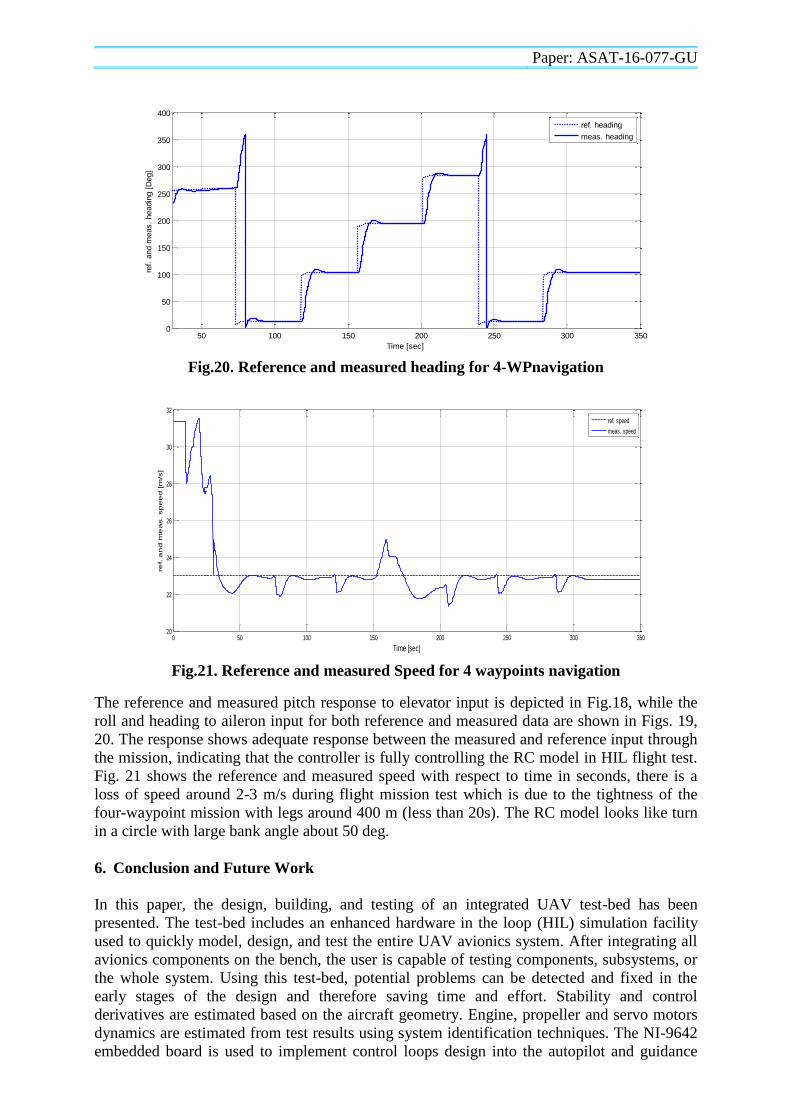
Fig.20. Reference and measured heading for 4-WPnavigation
Fig.21. Reference and measured Speed for 4 waypoints navigation
The reference and measured pitch response to elevator input is depicted in Fig.18, while the
roll and heading to aileron input for both reference and measured data are shown in Figs. 19,
20. The response shows adequate response between the measured and reference input through
the mission, indicating that the controller is fully controlling the RC model in HIL flight test.
Fig. 21 shows the reference and measured speed with respect to time in seconds, there is a
loss of speed around 2-3 m/s during flight mission test which is due to the tightness of the
four-waypoint mission with legs around 400 m (less than 20s). The RC model looks like turn
in a circle with large bank angle about 50 deg.
6. Conclusion and Future Work
In this paper, the design, building, and testing of an integrated UAV test-bed has been
presented. The test-bed includes an enhanced hardware in the loop (HIL) simulation facility
used to quickly model, design, and test the entire UAV avionics system. After integrating all
avionics components on the bench, the user is capable of testing components, subsystems, or
the whole system. Using this test-bed, potential problems can be detected and fixed in the
early stages of the design and therefore saving time and effort. Stability and control
derivatives are estimated based on the aircraft geometry. Engine, propeller and servo motors
dynamics are estimated from test results using system identification techniques. The NI-9642
embedded board is used to implement control loops design into the autopilot and guidance
50 100 150 200 250 300 3500
50
100
150
200
250
300
350
400
Time [sec]
ref.
and m
eas.
headin
g [
Deg]
ref. heading
meas. heading
0 50 100 150 200 250 300 35020
22
24
26
28
30
32
Time [sec]
ref. a
nd
me
as. sp
ee
d [m
/s]
ref. speed
meas. speed
Paper: ASAT-16-077-GU
system. RC Switch is used for multiplex between RC pilot and autopilot. Other test-bed
components are airborne telemetry, navigation sensors, batteries, and petrol engine (DA-50).
A ground station, for UAVs, is designed and built. The ground station has been developed
using LABVIEW software package. The designed interface includes gauges to monitor speed,
altitude, and aircraft attitudes. It also includes a map that shows the global position of the
aircraft. Finally, a GUI is used to upload commands directly to the aircraft.
7. References
[1] Amer AI-Radaideh, AI-Jarrah, M.A., and Dhaouadi, R., “ARF60 AUS-UAV Modeling,
System Identification, Guidance and Control: Validation Through Hardware in the Loop
Simulation”, Proceeding of the 6th International Symposium on Mechatronics and its
Applications (ISMA09), Sharjah, UAE, March 24-26,2009., pp. ISMA09-1- ISMA09-11.
[2] Barros, S. R., Givigi, S. N., Bittar, A., “Experimental Framework for Evaluation of
Guidance and Control Algorithms for UAVs”, Proceedings of COBEM, October 24-28,
2011, Natal, RN, Brazil pp. 123-133.
[3] Johnson, E. N, Fontaine, S., “Use of Flight Simulation to Complement Flight Testing of
Low-cost UAVs”, AIAA Modeling and Simulation Technologies Conference and Exhibit,
Montreal, Canada, Aug. 2001, pp. 2001-4059.
[4] Shawky, A., Grimble, M., Ordys, A., and Petropoulakis, A., “Modelling and Control
Design of a Flexible Manipulator Using State-Dependent Riccati Equation technique”,
Proceedings of the 7th
IEEE International Conference on Methods and Models in
Automation and Robotics, August, 2001, volume 1.
[5] Robert Nelson, Flight Stability and Automatic Control, McGraw-Hill, New York, 1989,
pp. 83-175.
[6] Roskam, Airplane Flight Dynamics and Automatic Flight Controls, Lawrence Roskam
Aviation and Corporation, New York, 2001, Part I.
[7] “AeroSim Blockset’’, Unmanned Dynamics, Date accessed 16/08/ 2006,
http://www.u-dynamics.com/aerosim/
[8] “Development of Autonomous Unmanned Aerial Vehicle Reshearch Platform: Modeling,
Simulating, and Flight Testing”, March 2006, Department of Aeronautics and
Astronautics USAF.
[9] “Introduction to Aircraft Stability and Control Course Notes for M&AE 5070”, 2011,
Sibley School of Mechanical & Aerospace Engineering Cornell University.
[10] Randy C. Hoover, “Fusion of Hard and Soft Computing for Guidance, Navigation, and
Control of Uninhabited Aerial Vehicles”, December, 2004, Ms. Science, Idaho State
University.
[11] Kamal, A. M., Bayoumy Aly, A.M., Elshabka, A., “Modeling, Analysis and Validation of
a Small Airplane Flight Dynamics”, (AIAA 2015-1138), Jan 2015, AIAA Modeling and
Simulation Technologies Conference, San Diego, California, USA, 10.2514/6.2015-1138.