hardware demonstration: frequency spectra of transients

1To be presented by John McCloskey at the IEEE International Symposium on Electromagnetic Compatibility, National Harbor, MD, August 7-11, 2017

John McCloskey

NASA/GSFC

Chief EMC Engineer

[email protected]

Hardware Demonstration:

Frequency Spectra of Transients

August 9, 2017

2017 IEEE International Symposium on Electromagnetic Compatibility

Jen Dimov

AS&D Inc. work performed for NASA/GSFC

EMC Engineer

[email protected]


Acronym List

CW Continuous Wave

dB Decibel

EMC Electromagnetic Compatibility

EMI Electromagnetic Interference

ESD Electrostatic Discharge

GSFC Goddard Space Flight Center

NASA National Aeronautics and Space Administration

NESC NASA Engineering and Safety Center


Introduction/Abstract

Radiated emissions measurements as specified by MIL-STD-461 are performed in the

frequency domain, which is best suited to continuous wave (CW) types of signals

Non-CW signals can potentially generate momentary radiated emissions that may be

missed with traditional measurement techniques

Single event pulses/transients (e.g. ESD type events)

Low repetition rate signals

“Bursty”/modulated signals

Recent real-life event:

A machine model ESD event occurred in the immediate vicinity of an antenna

connected to an integrated satellite receiver

We had to assess coupling relative to radio front-end transient damage threshold

This demonstration provides measurement and analysis techniques that effectively

evaluate the potential emissions from such signals in order to evaluate their impacts

to system performance, damage thresholds, etc.


This demo also touches upon…

Real-time spectral analysis

Narrowband vs. broadband signals

How your measurement technique can influence your

result (a touch of Heisenberg, perhaps?)

Analysis vs. test


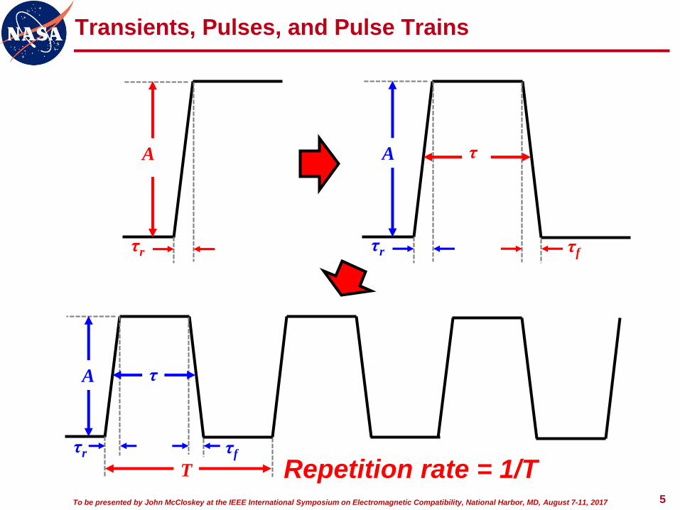
Transients, Pulses, and Pulse Trains

τ

τr τf

A

τr

A

τ

τr τf

T

A

Repetition rate = 1/T


Frequency Spectra of Repeating Pulse Trains

Well understood, characterized, and documented:

Clayton Paul, “Introduction to Electromagnetic Compatibility"

• Sections 3.1 and 3.2

NESC Academy Video: "Effects of Rise/Fall Times on Signal

Spectra“, J. McCloskey

• https://mediaex-server.larc.nasa.gov/Academy/Play/f16370c89d3d437fa193b4013dbb5a4f1d

Other NESC Academy videos:

https://nescacademy.nasa.gov/

Type “McCloskey” in search bar

https://mediaex-server.larc.nasa.gov/Academy/Play/f16370c89d3d437fa193b4013dbb5a4f1d

https://nescacademy.nasa.gov/


Trapezoidal Wave: Time Domain vs. Frequency Domain

TIME

DOMAINFREQUENCY

DOMAIN


Ideal Impulse (cont.)

TIME

DOMAIN

FREQUENCY

DOMAIN

tt0

δ(t)

f

F(f)


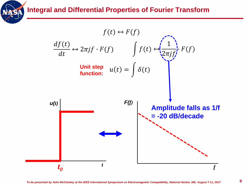
Integral and Differential Properties of Fourier Transform

𝑓(𝑡) ↔ 𝐹(𝑓)

𝑑𝑓(𝑡)

𝑑𝑡↔ 2𝜋𝑗𝑓 ∙ 𝐹(𝑓) න𝑓(𝑡) ↔

1

2𝜋𝑗𝑓∙ 𝐹(𝑓)

Amplitude falls as 1/f

= -20 dB/decade

tt0

u(t)

f

F(f)

𝑢 𝑡 = න𝛿(𝑡)Unit step

function:


Pulse Spectrum Dependence on Repetition Rate

Single pulse may be modeled as a pulse train taken in the limit as:

T → ∞ (f → 0)

For constant A, τ, τr, and decreasing repetition rate (increasing T):

Spacing of harmonics decreases proportionally

Duty cycle τ/T decreases proportionally

Amplitude of entire envelope decreases proportionally - WHEN MEASUREMENT

BANDWIDTH IS SUFFICIENT TO RESOLVE INDIVIDUAL HARMONICS


Demonstration 1:

Pulse Spectrum Dependence on Repetition Rate

Frequency spectra with the following constant values:

A = 1 V p-p

τ = 500 nsec

τr = τf = 4 nsec

Varying repetition rate: 1 MHz, 100 kHz, 10 kHz

1 kHz measurement bandwidth

Sufficient to resolve individual harmonics


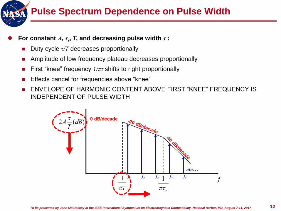
Pulse Spectrum Dependence on Pulse Width

For constant A, τr, T, and decreasing pulse width τ :

Duty cycle τ/T decreases proportionally

Amplitude of low frequency plateau decreases proportionally

First “knee” frequency 1/πτ shifts to right proportionally

Effects cancel for frequencies above “knee”

ENVELOPE OF HARMONIC CONTENT ABOVE FIRST “KNEE” FREQUENCY IS

INDEPENDENT OF PULSE WIDTH


Demonstration 2:

Pulse Spectrum Dependence on Pulse Width

Frequency spectra with the following constant values:

A = 1 V p-p

τr = τf = 4 nsec

T = 10 kHz

Varying pulse width: 500 nsec, 5 µsec, 50 µsec

1 kHz measurement bandwidth

Sufficient to resolve individual harmonics


MIL-STD-461G Table II

But…measurement bandwidth is not arbitrary…

Used in Demonstration 3


MIL-STD-461G Appendix A


Narrowband vs. Broadband?

Q: What defines a signal as “narrowband”?

A’s:

• When it has frequency content (e.g. harmonics) spaced sufficiently far

apart that the measurement bandwidth can properly resolve it

• When you change the measurement bandwidth and get the same result

Q: What defines a signal as “broadband”?

A’s:

• When it has frequency content (e.g. harmonics) spaced closer together

than the measurement bandwidth can properly resolve

• When you change the measurement bandwidth and the level changes

proportionately

IT’S ALL ABOUT BANDWIDTH!!!


Repetition Rate < Measurement Bandwidth

What happens when we decrease repetition rate below

measurement bandwidth?

Amplitude of entire envelope decreases proportionally

Spacing of harmonics decreases proportionally

Input filter with constant bandwidth sees constant broadband level

Input filter with constant

bandwidth greater than

harmonic spacing


Demonstration 3: Broadband Spectra for Repetition Rates

Lower than Measurement Bandwidth

Measure frequency spectra as indicated below using 2 methods:

Demo 3a: Standard spectrum analyzer mode using max hold

Demo 3b: Real-time spectrum analyzer mode

Frequency spectra

30 – 50 MHz as example frequency range

100 kHz measurement bandwidth per MIL-STD-461G Table II

Constant values: A = 1 V p-p, τ = 500 nsec, τr = τf = 4 nsec

Repetition rate

• 1 MHz stepped down to 100 kHz in 100 kHz increments

• 10 kHz, 1 kHz, 100 Hz, 10 Hz, 1 Hz…

Demo 3c: Change measurement bandwidth with fixed (low) repetition rate

Measured broadband signal is proportional to bandwidth


Implications...

When repetition rate is higher than measurement bandwidth:

Individual harmonics can be resolved

It is a narrowband signal

Changing repetition rate changes frequency spectrum proportionally

When repetition rate is equal to or less than measurement

bandwidth:

Individual harmonics cannot be resolved

It is a broadband signal

With constant measurement bandwidth, broadband frequency

spectrum is independent of repetition rate


Single Pulse or Low Repetition Rate Pulse Train

Broadband spectra of low repetition rate signals may be measured with real-time FFT

spectrum analyzer/receiver

If such a unit is not available, high frequency broadband spectrum envelope for low

repetition rate signals may be modeled as pulse train with effective repetition rate

equal to the measurement bandwidth

Effective repetition rate

= Measurement BW


Single Transient Model 1: Integral of Single Pulse

τr

A/τr

τr

A

τr

T Repetition rate = 1/T

Model single transition as

integral of single pulse

(A = area under curve)

A/τr


Single Transient Model 2:

Repeating Pulse Train with Same Characteristics as Transient

τ

τr τf

A

τr

A

τ

τr τf

T

A

Repetition rate = 1/T

Recall:

High frequency content

is independent of τ

τ is arbitrary


Example Spectral Comparison Between Models

A = 1 V p-p

τr = 20 nsec

τ = 400 nsec

T = 1 μsec𝑨𝟏 = 𝟐𝑨

𝝉

𝑻

𝑨𝟐 =𝟐𝑨

𝝉𝒓∙𝝉𝒓𝑻∙𝟏

𝟐𝝅𝒇=

𝑨

𝝅𝒇𝑻

𝑨𝟐 𝒇 =𝟏

𝝅𝝉=𝑨𝝉

𝑻


Example Spectral Comparison Between Models (cont.)

Above first “knee” frequency (1/πτ), spectrum for pulse train model

is 6 dB higher than integral of impulse model

Integral of impulse model (Model 1)

More accurate

Mathematically more cumbersome

Pulse train model (Model 2)

Mathematically simpler

Includes 2x actual number of transitions

Can use pulse train model and reduce by 6 dB to predict actual

broadband spectrum (or keep 6 dB margin in your pocket)


THANK YOU!

hardware demonstration: frequency spectra of transients

Documents