“haotic logic,” m.p. frank & e. debenedictis notes … submitted, the core simulator...

The title of our paper was kind of a mouthful, but we’re just calling this presentation “Chaotic Logic,” since that’s really the central idea here. The paper and talk are about a new way of thinking about how to do digital logic in nonlinear systems exhibiting chaotic dynamical behavior. This opens the door to the development of a new class of devices and circuits featuring extreme energy-efficiency.

I’ll explain later in the talk what these tangles are representing. (They look like random scribbles, but in fact they are simulation results.)

Acknowledgements: This work was done in the Non-Conventional Computing Technologies Dept. in the Extreme-Scale Computing Group at the Center for Computing Research, under the Science & Technology Divison of Sandia National Laboratories. Thanks to Stan Williams of HP for helping to inspire some of these ideas in Fall 2015 during the collaboration on the IEEE Sensible Machines whitepaper. Thanks to Sapan Agarwal and John Aidun for discussions and feedback on early writeups of these concepts. This work was supported by the LDRD and ASC programs in NNSA. Some of the Python code used in the simulator was previously developed for the COSMICiproject at the Astroparticle and Cosmic Radiation Detector R&D Lab (APCR-DRDL) in the FAMU Physics Dept., and was subsequently open-sourced.

“Chaotic Logic,” M.P. Frank & E. DeBenedictisICRC 2016, San Diego, 10/17/2016

Notes pages generated: 11/30/2016

What I’m going to do is first present the material that was in the paper, which reviewed the motivation and described the basic concept. In the months since the final paper was submitted, the core simulator framework was completed and early simulation results were obtained, and so I’ll go on to present those as well.



The line of work reported here (and in the accompanying paper) is motivated by a convergence of several different concerns. (We’ll discuss these motivations in in more detail in subsequent slides.)

• Looking beyond the specific characteristics assumed for CMOS-like technology, we would like to better understand what are the fundamental limits for the possibilities of computation at extremely low signal energies (very few kT, or even <<kT).

• Is it really the case that reliable computation becomes completely impossible given extremely low signal energies? Why or why not, exactly?

• When considering the fundamental thermodynamic limits on energy efficiency for irreversible computing implied by Landauer’s principle, we want to more clearly characterize how to properly apply the principle.

• What exactly are the meaning of terms like “information,” “state,” “transition” Need to be clear and correct on these when applying Landauer’s principle!

• When considering possibilities for logically-reversible computing, we would like to look beyond the usual approach of performing reversible logic over a long sequence of synchronous adiabatic transition stages…

• Can we eliminate the clocks, and update an entire logic net in one step?

• Finally, can we utilize chaotic, nonlinear dynamical systems for computing?



The first motivation for this line of work comes from communication theory. The Shannon channel capacity theorem fundamentally limits the maximum rate C at which information can be reliably communicated via a single continuous band-limited signal of given bandwidth B, given the ratio between average signal power S and noise power N (which is, in the worst case, white noise). The bound is derived essentially by simply counting the number of signal states which remain distinguishable given the magnitude of the noise perturbations. However, note that even when the noise power is of comparable magnitude to the signal power or greater, N S, the channel capacity is not zero. This is because, given a sufficiently long measurement period T, one may take a sufficiently large number k of independent samples (at the Nyquist sampling rate limit) such that the k-dimensional sphere of radius (S+N)1/2 of sample vectors for a signal of average power S+N has a much larger k-volume than the k-dimensional spheres of radius N1/2 representing the possible noise perturbation vectors with average noise power N,and thus many different non-overlapping “noise spheres” can be packed into the “signal volume.” Another way to say this is that over long enough time periods T, the random noise perturbations “average out” to an extent that the identities of at least 2CT different underlying signal “codewords” remain reliably distinguishable.

Note, however, that Shannon’s theorem is not saying anything about what the channel is doing to the signal (other than adding the random noise to it); it is only counting the numberof distinguishable signal states. Thus, the theorem remains entirely valid for a channel that deterministically (and reversibly) maps the input signals from an input code space to an output code space, in addition to adding the noise to them – since this does not change the number of distinguishable signals. These deterministic transformations can implement arbitrary reversible computations. Thus, Shannon’s theorem indicates that it ought to be possible to carry out reliable computation, as well as communication, using signals whose average energy (when sampled) has lower magnitude than the thermal energy, by using this same trick of “averaging out” the noise. (Also, note that Shannon’s theorem does not at all imply that the signal power, whatever it may be, must be dissipated.)

But how, in detail, can reliable computing below the noise floor be done? The following research explores one possible approach.



Motivation #2: Clarifying Landauer’s principle. Is Landauer’s lesson that “Any Boolean logic gate operation necessarily dissipates at least kT ln 2 energy?”

NO!!! That is an over-generalized statement of Landauer’s lesson.

Strictly speaking, that statement only applies in the special case of gates operating in isolation that irreversibly overwrite the logic value of their output nodes, if the value being overwritten has a probability of 50% of being different from the old value (from the mechanism’s perspective).

Rather, the following statement is the true essence of what Landauer is saying, and is what is actually true (irrefutably):

Whenever two or more distinct computational states (having nonzero probability) are merged (transformed to a single state), this causes a reduction in computational entropy, which (by the 2nd law of thermodynamics) must be compensated for by (at least) an equal increase in the entropy of non-computational degrees of freedom.

IMPORTANT: What is the meaning of “state” here?

Raises the question: Can we do logic without merging states?

Yes. That’s the concept behind reversible computing

Merging in only very-low-probability states also approaches the ideal of logical reversibility



This slide is just a historical note. We can trace the origins of our modern understanding of the informational foundations of physics back to Ludwig Boltzmann, who came to understand that physical entropy relates to probabilities, in the sense that ensembles of microstates having greater total probability contributed more to the total entropy of the system. In a series of papers, he derived his famous “H-theorem” showing that a certain quantity 𝐻 = 𝑓 log 𝑓, where f is a

probability density function over system configurations, decreases (becomes more negative) over time as a system (such as an ideal gas) evolves dynamically, as a result of nonlinear interactions between subsystems (e.g. colliding atoms) in the system, which tend to cause the probability distribution to disperse (become less peaked), and the average log f value to become more negative. This result was intended to explain the origin of the 2nd Law of Thermodynamics, where −𝐻 can be seen to correspond to entropy, which therefore increases. It could also be considered to have been an early precursor to the modern discipline of chaos theory (which we’ll say about more later). And crucially, it also anticipates the modern informational understanding of physics.

Note that if we assume that the state space is discrete, so that the probability density functions f become just probabilities p, and the integral becomes a summation, then we have 𝐻 ∝ σ𝑝 log 𝑝, which, if we set the proportionality constant to −1 instead of 1, becomes exactly Shannon’s entropy formula. (In fact, Shannon credits Boltzmann in his work.)

Around 1900, Planck, in attempting to understand blackbody radiation, assumed the discreteness of states, and also introduced the constant k into Boltzmann’s formula, to translate the dimensionless logarithmic units into conventional physical entropy units such as Joules/Kelvin. (Planck also introduced his constant h in the same paper; note that both constants arose out of Planck’s assumption that physical states are discrete.) It was then recognized that, since, at equilibrium, all microstates with a given energy become equally likely, Boltzmann’s formula reduces in that case to simply S = k log W, where W=1/p is the number of discrete states, or ways of arranging the system. This formula is carved on Boltzmann’s tombstone in his honor.



In Boltzmann’s day, how exactly to enumerate his inferred microscopic arrangements or states remained mysterious…

In fact, it was exactly addressing this problem that led Planck to introduce k(“Boltzmann’s constant”) and h (“Planck’s constant”), which subsequently led to the entire development of quantum theory.

Modern quantum theory teaches us that any two orthogonal state vectors of a quantum system comprise mutually distinguishable states…

Distinguishable states are what is relevant for counting states w.r.t. characterizing the entropy/information content of a system

Maximum entropy of a system = log(dimensionality of its Hilbert space)

However, another important realization from quantum theory is that, in general, a state may be a spatially-extended entity…

It is not always just the state of a single atomic, localized system..

C.f. entangled states of quantum systems: EPR pairs, “Schrödinger’s cat” states, collective states of Bose-Einstein condensates, superconductors/superfluids

In general, when applying Landauer, we need to pay attention to what happens the state of the whole system, in a holistic sort of analysis…

Don’t always insist on decomposing the system into subsystems!



One frequently sees descriptions of Landauer’s limit which claim something like, “every Boolean logic gate must necessarily dissipate kT ln 2 on every logic operation.” And much of the literature on reversible computing claims that, “To avoid Landauer’s limit, we cannot use Boolean gates at all, but instead must replace them with fully-reversible gates such as Fredkin or Toffoli gates.” Neither of these statements is true. It is true that traditional implementations of Boolean gates are irreversible. But that is not because of the function that these gates are computing. That “function” is ultimately just a relation between input states and valid output states. The irreversibility of traditional implementations of Boolean gates is simply because the method of operation of the gate is to destructively overwrite the output node with a new value (irreversibly discarding its old value) whenever the inputs change (which is assumed to happen instantaneously). However, if we imagine the output smoothly changing to its new value while the input changes to its new value, there is nothing that is necessarily irreversible about this. Even for a complex multi-layer network such as shown above, the transition of the state of the whole network from old state to new state can be represented as follows (inputs in brackets, outputs in parens):

[N6N7N8]N1N2N4(N3N5): [000]000(00) [111]011(11)

Note that if we don’t assume that these gates are implemented in the usual way there is no merging of states necessarily happening here. We are going from one old holistic state of the whole network to oneuniquely-determined new holistic state of the whole network, where the entire transition is determined by the fact that we are taking the inputs from [000] to [111] in this transition. The same would apply for any other externally-controlled transition of the inputs. Overall, if the gates are working correctly, this whole network only has 23=8 distinct digital states, not 28=256 distinct digital states, because the gate outputs do not represent independent information from the inputs. However, traditional CMOS implementations of Boolean gates are non-ideal for taking advantage of this fact, because of the way they operate: They necessarily move a substantial charge (CV), where C is output node capacitance over a substantial voltage drop V whenever they cycle their output node from 0 to 1 and back. We need to consider other ways of doing logic.



Motivation #3: Simplifying reversible computing. “Traditional” implementations of reversible computing in (e.g.) adiabatic CMOS did not attempt to radically depart from traditional voltage-coded logic. Instead, they avoided the CV2 losses by updating the network reversibly in a sequence of shorter adiabatic update stages, during each of which the CV charge is moved over only over a much smaller voltage drop due to gradually-ramping supply voltages. The simplest approach for this (due to J. Storrs Hall, and relating to underlying concepts from Bennett) is the retractile cascade, in which (1) gate inputs to the first logic stage are changed adiabatically from a default (old) value to new values, then (2) gate outputs from the first logic stage are changed adiabatically from old to new values, under external control, (3) the outputs of subsequent stages of logic outputs are also changed, one at a time, (4) the final output is latched, (5) the logic outputs are adiabatically rolled back, in reverse order. In the end the entire network is returned to the initial state, after which new inputs can be provided.

This was fine for combinational (feed-forward) logic, and later work by Younis and Knight showed how to implement arbitrary pipelined, sequential logic in adiabatic CMOS as well, again through an explicitly-controlled staging sequence.

However, all these methods have a high design-complexity overhead, due in part to the large number of externally-supplied “power/clock/control” signals that are used to sequentially drive the logic transitions. Can we somehow do away with this overhead, and update even complex logic networks reversibly in a single step? That this was possible was suggested by the existence of complex gates in various adiabatic circuit styles that performed the equivalent of multiple stages of logic in a single gate. Additionally, work on quantum-dot cellular automata (QDCA) suggested that updating multi-layer logic in a single adiabatic transition was possible in a quantum model of reversible computing. Is it also possible classically?



Motivation #4. How to cope with chaos. If we ever want to approach the ideal of nondissipative computing, we have to face this issue. Complex undamped (conservative, nondissipative) nonlinear dynamical systems typically (almost ubiquitously) exhibit dynamical chaos, meaning roughly, exponential sensitivity to initial conditions. That is, given two extremely similar initial states, any initial uncertainties tend to be amplified over time, so that the long-term trajectory is completely unpredictable. As mentioned earlier, this type of behavior (of increasing uncertainty) was alluded to early on by Boltzmann in his H-theorem. The unpredictable dynamics manifests itself as random-looking fluctuations or noise in the dynamical degrees of freedom. We can assign an effective temperature T to the dynamical degrees of freedom, such that the average dynamical energy per degree of freedom is kT(typically ½kT of this energy is kinetic, associated with momentum-type variables, and ½kT is potential, associated with position-type variables). In nanoscale systems, these unavoidable chaotic fluctuations are characterized as thermal noise. Chaos can be viewed as the primary origin of entropy increase at the nanoscale, although even linear quantum systems can also experience increasing uncertainty due to decoherence if there is interaction with an unknown external environment. There is a whole field of quantum chaos, but we won’t get into it here.

Anyway, the basic point is that it seems that chaos is an unavoidable feature of nanoscale dynamical systems, if we don’t want to damp out the fluctuations via dissipative processes (i.e., by starting out in a nonequilibrium state, and then allowing the system’s energy to thermalize as it relaxes towards an equilibrium state). Is it even possible to compute at all in a chaos-dominated regime? This relates, of course, to our motivation #1 from Shannon, of whether it is possible to compute with very low signal energies, below the “noise floor.”



What are some potential advantages of utilizing chaotic dynamical systems for computation?

In a conservative chaotic system, the strange attractor to which the dynamics converges represents a thermodynamic equilibrium state

Once converged onto the attractor, there is no further energy dissipation

This remains true even if the system is interacting with an external thermal environment once the system and environment temperatures have equilibrated, due to the fluctuation-dissipation theorem

Yet, the identity of the attractor reflectsinformation about the initial state andthe time-series of external forcings that are being applied to the system

Convergence to the attractor automatically computes a certain function of these inputs!

Possibly a useful one…

Cheaply maps a simple input into a much higher-dimensional space of trajectories

This can be useful as a basis for machine learning, as in reservoir computing



We have set the stage, and are now ready to present our proposal for a new concept of “chaotic logic” which addresses all of the aforementioned motivations.

We start with a completely conventional structure of a combinational Boolean logic network, such as the one we illustrated earlier, which was a so-called “full adder” – it sums three input bits (each 0 or 1) to produce a two-bit total, which can represent any of the possible sums, ranging from 0 (002) to 3 (112).

However, instead of implementing this with CMOS gates and voltage-coded nodes, we’re going to do something completely different.

A “node” will be represented by some dynamical degree of freedom – any continuous generalized-position type coordinate. It does not have to be a literal position of anything, it can be any dynamical variable – e.g., the rotation angle of a nanomechanical armature, or the current in a superconducting loop. (Actually, supercurrents are quantized, but at large enough values are nearly continuous.) Two specific values of the position coordinate will be assigned to represent “logic 0” and “logic 1,” respectively.

Meanwhile, we will implement a “gate” as a classical Hamiltonian interaction function, representing a potential energy that varies as a function of the “positions” of the nodes impinging on that gate. The shape of this potential energy function will be crafted so that when the inputs are at valid logic values, the energy is minimized when the output is at the corresponding valid logic value. When the output is at the incorrect logic value, the energy will be higher. For other values of input and output nodes, we want to smoothly interpolate between these cases.

Note that the Hamiltonian representation means that this is a conservative dynamical system – its total energy (given by the sum of kinetic and potential Hamiltonian terms) is constant.

Given any initial state of the network, we just let it evolve. Since this is a complex, nonlinear conservative dynamical system, we predict it will exhibit chaotic, thermal behavior, with an effective temperature given by the energy per degree of freedom. However, we also predict that over sufficiently long time periods, the average value of any given node will round to the correct logic value that it should have (according to the structure of the Boolean network) given the average value of the input nodes. The input nodes can be made to average to their desired values by an externally-supplied bias potential, which can be considered a memory cell (not explicitly represented in this diagram).

We can cause this system to “compute” by simply switching the input biases to a new value. If this switching is done rapidly and irreversibly (without regards to the prior value), this thermalizes the energy that was injected to switch the input biases (note however that the dissipation does not depend on the number of other nodes in the network, since energy is only being added at the inputs). (This comports with Landauer, since remember the entire network has only 23 valid states, not 28, so only 3 bits are being forgotten when the inputs get irreversibly overwritten.) Alternatively, if the switching is done gradually and reversibly (adiabatically), smoothly transitioning it from old to new state, then this can be done with no heating of the system, and no energy dissipation. And all in a single step, with no need to clock in a sequence of transitions of individual logic stages.




13

This slide is just a review of basic classical Hamiltonian mechanics, for those who aren’t familiar with it. We will use canonical coordinates, meaning we describe the system in terms of generalized-position type variables, each of which has an associated conjugate generalized momentum variable. The system’s total Hamiltonian is a function of all these variables, which in our case is expressed as a sum of terms representing the various kinetic and potential energies at work in the system. The system’s dynamics is then fully determined by Hamilton’s equations, which simply say that the time-derivative of any position variable is given by the partial derivative of H with respect to the conjugate momentum variable, and the time-derivative of any momentum variable is given by the negative of the partial derivative of H with respect to the conjugate position variable. Given conventional forms for kinetic and potential energy functions, these equations reduce to Newton’s laws.

Incidentally, Hamiltonian mechanics remains functional in quantum mechanics as well, except that there, the position and momentum variables take the form of linear operators (“observables”) which apply to the quantum state vector (a.k.a. wavefunction) and scale each position or momentum basis vector by a scalar factor representing what the measured value of the variable would be in that case. In the quantum domain, Hamilton’s equations reduce to Schrodinger’s equation, which determines quantum time evolution (and this in fact is how Schrodinger derived his equation historically).

Indeed, Hamilton’s framework works for all known fundamental physical theories, including also classical electrodynamics, special and general relativity, and quantum field theory. Note that Hamilton’s equations are reversible.


This is just an illustration of a potential energy function that can be used to represent a NOT gate. Here, the X coordinate represents the input variable, the Y coordinate (going back into the figure) represents the output variable, and the vertical axis is the energy. Note that the minimum-energy “valley” includes the points (X=0, Y=1) and (X=1, Y=0). It also includes all other points along the line that includes these two – so it under-constrains the input and output nodes. However, given any fixed value for the input node, there is a single minimum-energy value for the output. The shape of the function is quadratic in X or Y, which is convenient for applying the equipartition theorem. (Quadratic terms in the Hamiltonian all get an equal average energy of kT/2 at equilibrium.)



Potential energy surfaces for two-input gates are more difficult to visualize, since they range over a three-dimensional configuration space (the values of the two inputs and one output). However, here are some equations that will work. These are also quadratic in the state variables.

Note that when the coordinate values are 0,1 and are consistent (satisfy the logical equation for the gate), the numerical equations on the right are true, and the expressions in parentheses evaluate to 0, minimizing the value of the interaction function (the “stress energy”) at 0. When the coordinate values are incorrect (but still at 0,1), the equations on the right are violated by ±1, and the stress energies evaluate to ½eGATETYPE.

The eGATETYPE constants parameterize the energy scale of the gate interactions.

At incorrect logic values, the gate’s potential energy above its minimum, or “stress” energy, will be ½ this constant. Rough equiv. of “signal energy” in this system.

In the experiments shown here, the energy scales e of all gates were set equal to 𝑘𝑇.

At thermal equilibrium, by the equipartition theorem, every gate will have an average stress energy of ½𝑘𝑇. (And every node will also have an average kinetic energy of ½𝑘𝑇.)

Thus the magnitude of “thermal noise” is equal to that of the “logic signal” ½𝑘𝑇. SNR=1.



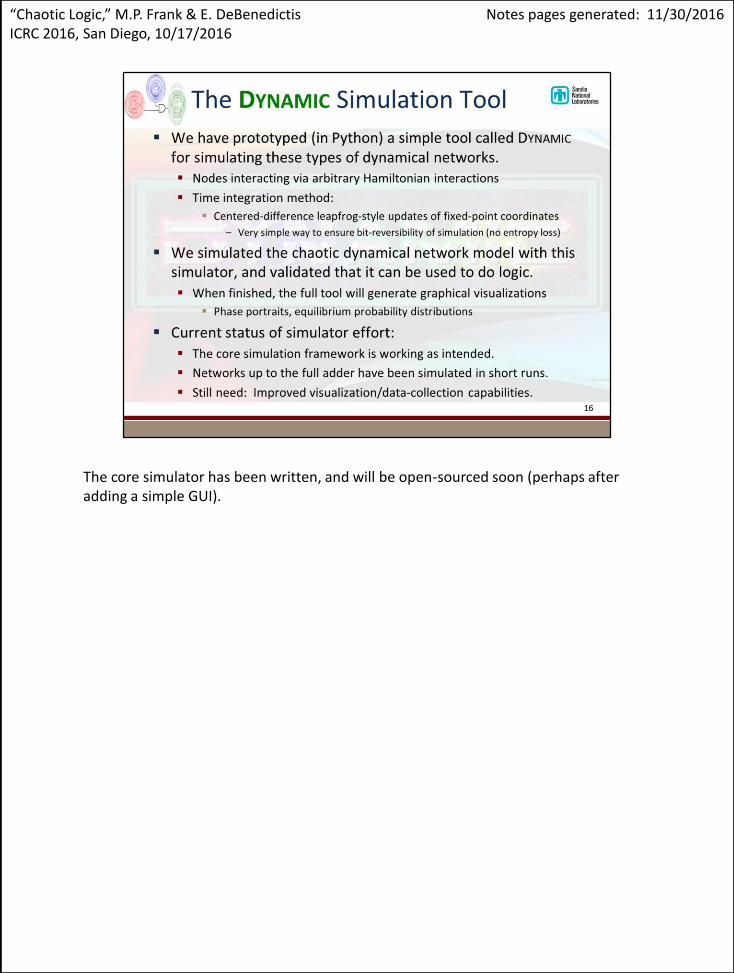
The core simulator has been written, and will be open-sourced soon (perhaps after adding a simple GUI).



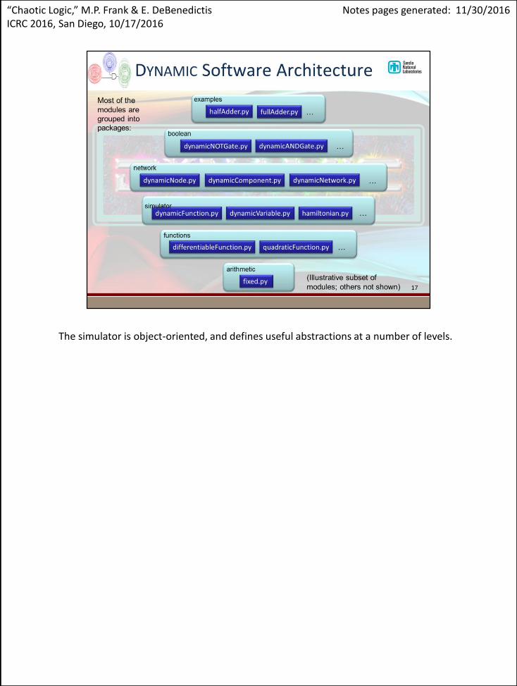
The simulator is object-oriented, and defines useful abstractions at a number of levels.



You can see here the first result, obtained for a simple dynamic network, consisting of a memory element feeding a NOT gate. In this case the input was biased to logic 0, so the output should be a 1. Note that the magnitude of the variability in both input and output values is comparable to or greater than the logic signal amplitude (which ranges from 0 to 1). (Actually the variability in the input is a little less, since it is constrained by two potentials at roughly equal energy scales, while the output is only constrained by one potential.) Yet, the average value of both input and output coordinates over time is very close to the nominal level. This illustrates that computed information can be reliably conveyed despite having a noise power level that is comparable to or greater than the signal power, i.e., with an

SNR <= 1.



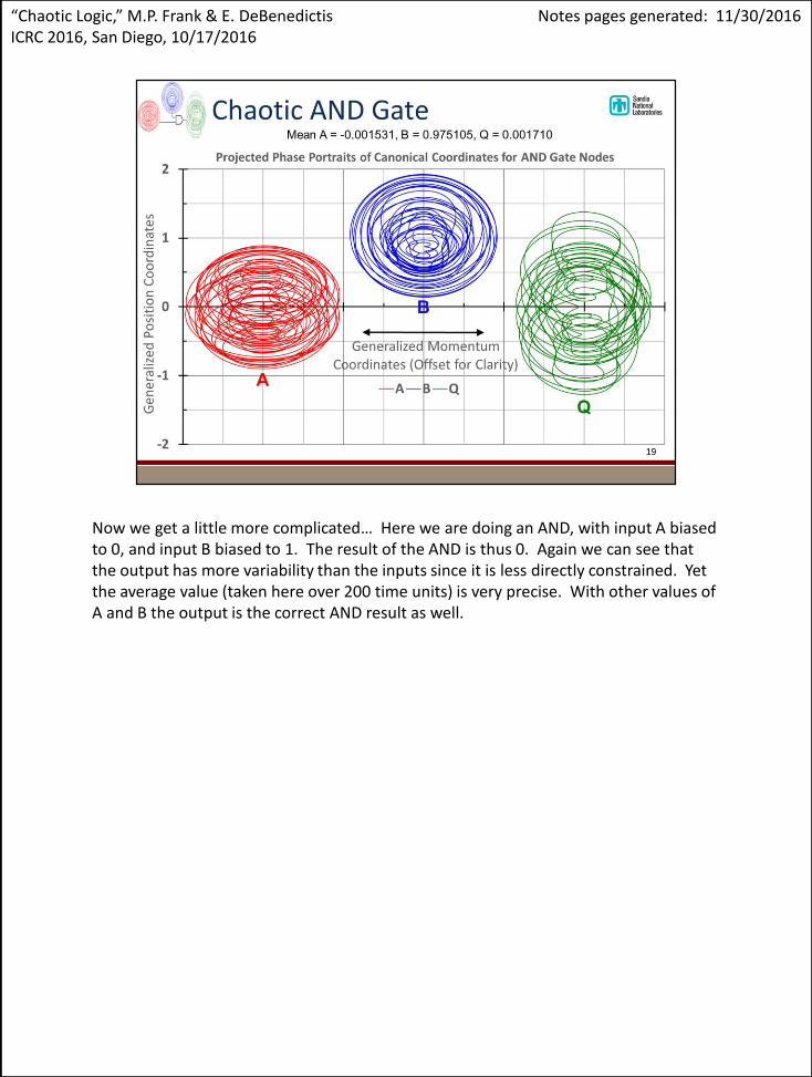
Now we get a little more complicated… Here we are doing an AND, with input A biased to 0, and input B biased to 1. The result of the AND is thus 0. Again we can see that the output has more variability than the inputs since it is less directly constrained. Yet the average value (taken here over 200 time units) is very precise. With other values of A and B the output is the correct AND result as well.



The timeline of fluctuations shows that there is a strong temporal correlation between input A (red) and the output (green). This is unsurprising since, when input A goes to 1, the nominal output of the AND also goes to 1, since B is being held at 1.



Here’s a slightly more complicated network, and we also show the complete equation for its Hamiltonian to illustrate how it is put together. Note we simply add together the terms for the different gates. Here we have set the gate stress-energy scaling factors to unity, eAND = eXOR = 1, and omitted them from the formula for clarity. The memory cells are biased via a quadratic potential as shown. The logic values illustrated correspond to bias values bi = 1.



Results for the half-adder. Note that having more nodes results in more variability for the output nodes. This can be interpreted as due to the fact that having more degrees of freedom, which are only constrained relatively to each other, results in a greater entropic term ST in the total free energy of the system. In other words, there is more total entropic “pull” to explore the variability available in the state space. Thus we can see long excursions in which the AND and XOR outputs wander away from their nominal logic values. However, the whole network is ultimately still constrained by the logic values of the inputs, and so the average values over the 200 time units (20,000 steps of size 0.01) are still correct.



This just shows that the rounded logic values were correct in experiments performed over all four input cases. However, there was one case that was just barely correct. We are getting near the limits of what can be done reliably given the run length we used. This is telling us that we can expect more complex networks will take longer to get reliable values out of.



And finally, a full adder, which is the network that we started with. Again, with more nodes, the excursions away from the nominal logic values are getting longer.



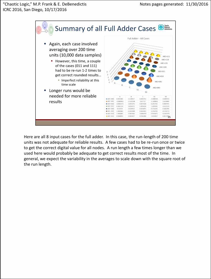
Here are all 8 input cases for the full adder. In this case, the run-length of 200 time units was not adequate for reliable results. A few cases had to be re-run once or twice to get the correct digital value for all nodes. A run length a few times longer than we used here would probably be adequate to get correct results most of the time. In general, we expect the variability in the averages to scale down with the square root of the run length.



If we want to prevent node coordinates from wandering far outside the range (0-1) of valid logic values, one simple way to do this is by adding another potential function to each node. We tried this, using a simple quartic double-well potential for which the stress-energy of valid logic levels is 0. This worked effectively to constrain the excursions, but did not seem to significantly improve the time to achieve valid averages, and may even have worsened it – this perhaps being because the steep “walls” of this double well, compared to the potential barrier between logic states, seem to have the effect of causing the node to bounce over to the wrong state more often.

There is another problem with adding double-well potentials, especially if we raised the barrier height, which is that it could significantly increase the time required for an adiabatic transition, by lengthening the relaxation timescale for transitioning to the “preferred” (lowest-energy) state distribution.



Next steps. This slide is pretty self-explanatory.



Conclusions. Self-explanatory



“haotic logic,” m.p. frank & e. debenedictis notes … submitted, the core simulator...

Documents