handling uncertain data in subspace detection

Handling uncertain data in subspace detection

Leandro A.F. Fernandes a,n, Manuel M. Oliveira b

a Instituto de Computação, Universidade Federal Fluminense (UFF), CEP 24210-240 Niterói, RJ, Brazilb Instituto de Informática, Universidade Federal do Rio Grande do Sul (UFRGS), CP 15064, CEP 91501-970 Porto Alegre, RS, Brazil

a r t i c l e i n f o

Article history:Received 21 June 2013Received in revised form4 April 2014Accepted 9 April 2014

Keywords:Hough transformUncertain dataSubspace detectionShape detectionGrassmannianGeometric algebraParameter space

a b s t r a c t

Experimental data is subject to uncertainty as every measurement apparatus is inaccurate at some level.However, the design of most computer vision and pattern recognition techniques (e.g., Hough transform)overlooks this fact and treats intensities, locations and directions as precise values. In order to takeimprecisions into account, entries are often resampled to create input datasets where the uncertainty of eachoriginal entry is characterized by as many exact elements as necessary. Clear disadvantages of the sampling-based approach are the natural processing penalty imposed by a larger dataset and the difficulty ofestimating the minimum number of required samples. We present an improved voting scheme for theGeneral Framework for Subspace Detection (hence to its particular case: the Hough transform) that allowsprocessing both exact and uncertain data. Our approach is based on an analytical derivation of thepropagation of Gaussian uncertainty from the input data into the distribution of votes in an auxiliaryparameter space. In this parameter space, the uncertainty is also described by Gaussian distributions. In turn,the votes are mapped to the actual parameter space as non-Gaussian distributions. Our results show thatresulting accumulators have smoother distributions of votes and are in accordance with the ones obtainedusing the conventional sampling process, thus safely replacing them with significant performance gains.

& 2014 Elsevier Ltd. All rights reserved.

1. Introduction

Voting-based techniques for fitting instances of a model toexperimental data are widely used in computer vision, patternrecognition and image processing. The most popular of theseapproaches is undoubtedly the Hough transform (HT). It was firstdesigned for detecting the straight lines that best fit points on theplane [1,2]. Later, the HT was specialized for detecting otheranalytical shapes, such as circles, parabolas and ellipses, and alsogeneralized for detecting arbitrary non-analytical shapes in images[3,4]. More recently, a generalization of the HT concept has beenpresented to detect any data alignment that can be representedanalytically and characterized as a linear subspace embedded inspaces with arbitrary dimensionality [5].

The HT works by mapping each primitive from the input datasetto points (in a parameter space) representing the shapes potentiallypassing through that primitive. Thus, shape detection is convertedinto the problem of identifying peaks in an accumulator array

representing the discretized parameter space. The strong aspects ofthe HT are its robustness to noise, clutter, and missing data.However, improper discretization of the parameter space may leadto unsharp or multiple peaks of votes [6,7]. In particular, if thediscretization is too fine, votes are likely to fall in neighboring bins,thus reducing the visibility of the main peaks. This problem getsaggravated when experimental data, which often contains errorsdue to imprecisions in the measuring instruments, are treated asexact entries. For instance, raster images captured by digitalcameras are resolution dependent. Likewise, computed tomographycaptures images of regularly spaced slices of a subject and hencerepresents inter-slice data by some approximation. Another sourceof uncertainty is the error associated with the estimation of the realcamera parameters, which are usually obtained using image-basedcalibration procedures. Although uncertainty is intrinsic to experi-mental data, this fact has been neglected by most researchersduring the development of shape and subspace detectors due to thedifficulty of handling it. If the HT voting procedure does not takeinto account the uncertainty present in the input data, the resultingaccumulator array is likely to contain spurious peaks of votes,making the identification of the actual peaks more difficult. Thequality of the detection procedures can be improved by consideringthe role of uncertainty in the detection mechanisms.

In this paper we extend the mapping and voting procedurespresented in [5] to handle input containing Gaussian distributed

Contents lists available at ScienceDirect

journal homepage: www.elsevier.com/locate/pr

Pattern Recognition

http://dx.doi.org/10.1016/j.patcog.2014.04.0130031-3203/& 2014 Elsevier Ltd. All rights reserved.

n Corresponding author. Tel.: +55 21 2629-5665; fax: +55 21 2629-5669.E-mail addresses: [email protected] (L.A.F. Fernandes),

[email protected] (M.M. Oliveira).URLS: http://www.ic.uff.br/� laffernandes (L.A.F. Fernandes),

http://www.inf.ufrgs.br/�oliveira (M.M. Oliveira).

Please cite this article as: L.A.F. Fernandes, M.M. Oliveira, Handling uncertain data in subspace detection, Pattern Recognition (2014),http://dx.doi.org/10.1016/j.patcog.2014.04.013i

Pattern Recognition ∎ (∎∎∎∎) ∎∎∎–∎∎∎

www.sciencedirect.com/science/journal/00313203

www.elsevier.com/locate/pr

http://dx.doi.org/10.1016/j.patcog.2014.04.013



mailto:[email protected]

mailto:[email protected]

http://www.ic.uff.br/~laffernandes

http://www.ic.uff.br/~laffernandes

http://www.inf.ufrgs.br/~oliveira

http://www.inf.ufrgs.br/~oliveira





uncertainty. The extended mapping procedure is based on first-order error propagation analysis [8]. It propagates the uncertaintyof each input element throughout the computations into anauxiliary parameter space where the uncertainty is described bya multivariate Gaussian distribution (Fig. 1b). In turn, such dis-tribution is mapped to the actual parameter space by the extendedvoting procedure. This lends to warped (non-Gaussian) distribu-tions of votes in the accumulator array (Fig. 1a) resulting inaccurate distribution of votes over the bins.

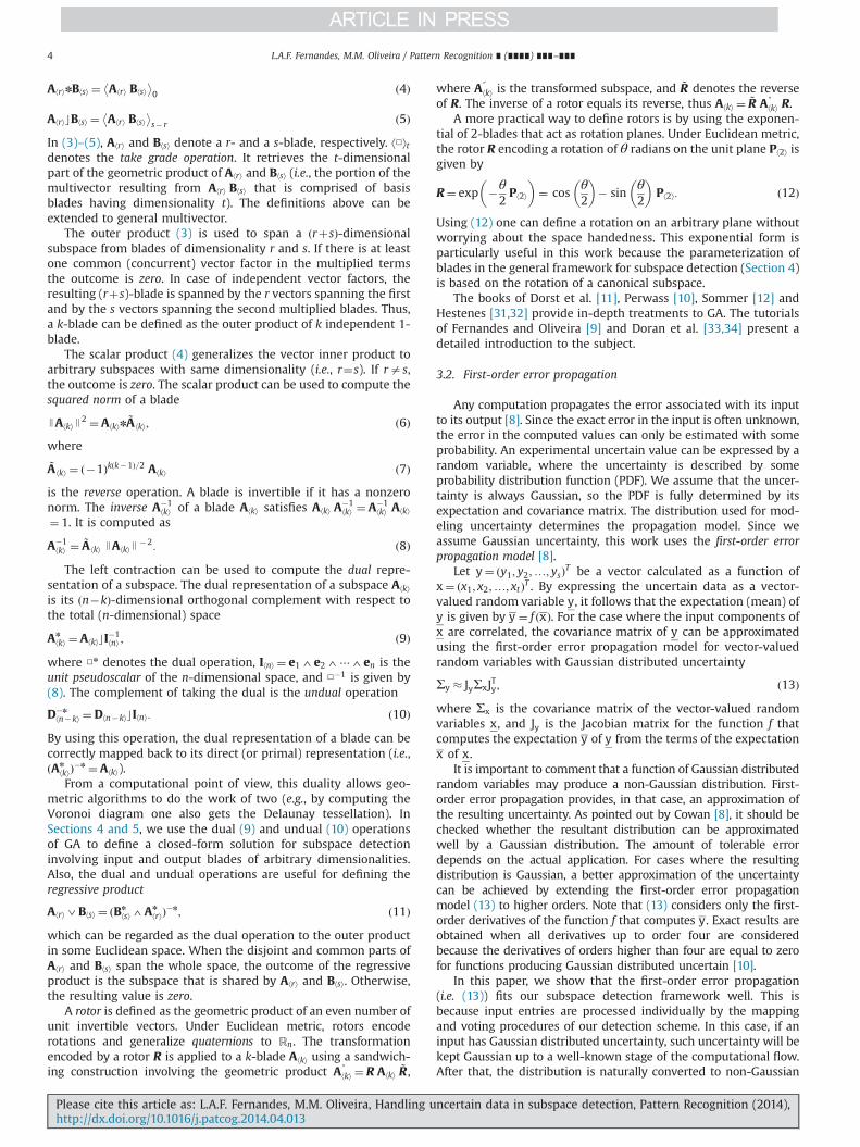
In order to handle uncertain data, existing voting-based tech-niques need to be applied to datasets that replace the actualuncertain input entries by as many samples as needed to char-acterize the distribution of uncertainty of each original entry. It isclear that such an approach imposes a processing penalty as thenumber of samples increase. Also, the smoothness of the resultingaccumulator array may be affected even when a large number ofsamples is generated (Fig. 5f). Our approach, on the other hand,treats each original uncertain input entry directly and propagatesits uncertainty throughout the computation chain, producingsmoother distributions of votes (Fig. 5c).

Our technique can be applied without changes and using a singleimplementation to the detection of all kinds of data alignmentsrepresentable as linear subspaces in any complete metric spaces.When the subspaces are interpreted as shapes, our formulationbecomes a general analytical shape detector that outperforms con-ventional HTs by being able to concurrently detect multiple kinds ofshapes, in datasets containing multiple types of data.

The central contribution of this paper is a more flexible votingscheme for the detection framework presented in [5]. It can handleboth exact data as well as data containing Gaussian-distributeduncertainties. In addition, we define an auxiliary space where theuncertainty of p-dimensional subspaces residing in some n-dimensional space is related to the uncertainty of r-dimensionalrandom subspace under first-order error propagation, for 0rrrn. This interesting property may lead to new insights into howto extend other subspace-clustering techniques to include errorpropagation into their formulations.

We formulate our subspace detector using geometric algebra[9–12], tensors [13], and error theory [8]. In order to validate it,we performed three sets of experiments that verify that ouruncertain-based voting scheme generates the expected votingdistributions. As a result, our technique reduces the scatteringof votes in the accumulator, lending to superior detection results.

2. Related work

Linear subspace learning (LSL) techniques aim to find linearprojections, of sets of training samples, satisfying some optimalitycriteria [14]. They map input data from a high-dimensional spaceto a lower-dimensional one where space partitioning and cluster-ing can be performed more conveniently. Principal componentanalysis (PCA), linear discriminant analysis (LDA), general aver-aged divergence analysis (GADA) [15,16], and locality preservingprojections (LPP) [17] are examples of LSL algorithms. Isomaps[18], locally linear embedding (LLE) [19], and their variations, suchas the local linear transformation embedding (LLTE) [20], extendthe dimensionality-reduction problem to dataset entries that lie innonlinear-manifold structures [21]. Recently, Zhou and Tao for-mulated the double shrinking model (DSM) [22], which aims tocompress data by simultaneously shrinking both dimension-ality and cardinality. All those techniques use points or vectorsin Rn as input. Multilinear subspace learning (MSL) techniques arehigher-order generalizations of LSL [23]. They use nth-ordertensorial samples as input data, thus enhancing their representa-tion power. When used for clustering, the goal of all dimension-ality-reduction techniques is to simplify the identification ofnearby entries.

In contrast to dimensionality reduction techniques, our approachaims to find the p-dimensional subspaces that accommodate asmany database objects as possible. Thus, it can be seen as a sub-space-clustering approach (see [24] for a review of such techni-ques). A key difference is that, with the exception of [5], all existingsubspace-clustering techniques are tailored for specific applicationsor input data types. Günnemann et al. [25] has recently proposedthe first subspace clustering approach for uncertain data. Theirtechnique is designed to detect linear subspaces aligned to the axisof the space where input uncertain points reside. Our approach, onthe other hand, inherits from [5] the ability to systematically adaptitself to handle r-dimensional input subspaces (0rrrn). In con-trast to our previous approach [5], the proposed technique wasdesigned to handle input entries containing Gaussian distributeduncertainty.

As pointed out in [5], our voting-based solution is a general-ization of the HT. The literature covering applications and varia-tions of HT-based techniques is vast [3,4]. The following sectionfocuses on techniques that, like ours, treat each input entry assome distribution during the voting procedure.

Fig. 1. The red spots in (a)–(c) represent the uncertainty of a given input blade. The distribution is shown as points computed by sampling the input blade according to itsGaussian distributed uncertainty and mapping each sample to P2 (a) and to A2 (b). The envelopes in (a) and (b) were obtained analytically by our approach. The points Θi

faceat the center of the bin's face (a) are mapped to the open affine covering for Gð2;3Þ as points aiface (b). In turn, the points aiface are mapped to the basis defined by theeigenvectors of the probability distribution (c). An axis-aligned bounding box is computed for aiface in such a basis. The number of votes to be incremented to a given bin ofthe accumulator array is proportional to the weight of the input blade and the probabilities of an intended p-blade be inside of the box. (For interpretation of the referencesto color in this figure caption, the reader is referred to the web version of this paper.)

L.A.F. Fernandes, M.M. Oliveira / Pattern Recognition ∎ (∎∎∎∎) ∎∎∎–∎∎∎2





2.1. Uniform distribution of uncertainty

O'Gorman and Clowes [26] set a uniform distribution ofuncertainty on the angular parameter of the normal equation ofthe line in order to limit the amount of bins that are incrementedfor each input pixel during the voting procedure. By doing so, eachinput point votes for a subset of the sinusoidal line resulting fromits mapping to the parameter space. Kimme et al. [27] use a similaridea to reduce the amount of votes spread in the detection ofcircles.

Cyganski et al. [28] use unit-area squares corresponding tofeature pixels instead of lattice coordinates. They show thatmapping square pixels to the parameter space of the slope-intercept form of the line results in a convex region that can beefficiently stored in a new data structure proposed in [29].

In contrast to these techniques, our formulation assumesGaussian (as opposed to uniformly) distributed uncertainty inthe input. Moreover, it is not tailored to a single kind of inputand, therefore, is a more general and flexible solution.

2.2. Gradient weighted Hough transform

Inspired by the optimization proposed in [26], van Veen andGroen [6] designed a weighting function to map an input pixel tothe accumulator array taking into account the gradient of the pixelto limit the number of bins receiving votes. With their function, adifferent weight is given to each vote according to a Gaussiandistribution centered on the angular parameter computed fromthe gradient angle of the point on a reference line with knownnormal direction.

Our approach also uses a weighting function for distributingvotes in the accumulator array. For this, we use first-order errorpropagation to compute the appropriate vote distribution to eachmapped entry.

2.3. Kernel-based Hough transform

The use of first-order error propagation in HT was introducedby Fernandes and Oliveira in the context of Kernel-Based HT (KHT)[30]. The approach operates on clusters of approximately collinearedge pixels. For each cluster, votes are cast and weighted using anoriented elliptical-Gaussian kernel that models the uncertainty ofthe best-fitting line with respect to the cluster. This lends to amuch cleaner voting map that is robust to the detection ofspurious lines, and allows a software implementation to performin real time.

The pipeline presented in [30] is specifically designed to detectstraight lines from image pixels. The present work, in contrast,extends the framework described in [5] to handle uncertaintyin the detection of arbitrary shapes. It is independent of thegeometric properties of the data alignments to be detected, andhandles heterogeneous datasets comprised by uncertain inputentries, and with possibly different dimensionalities and geome-trical interpretations.

It is important to note that the approach introduced in thispaper is not intended to perform in real-time like the KHT. Theperformance of the KHT results from an efficient clusteringprocedure and a culling strategy that avoids voting for kernelsthat are less likely to result in peak formation. Their generalizationto our technique is a promising direction for future exploration.

3. Mathematical background

In this section we briefly introduce the mathematical back-ground used in the paper. A more detailed introduction to these

topics can be found in the provided references. SupplementaryMaterial A summarizes the notational convention.

3.1. Geometric algebra

The Clifford algebra of a vector space over a field of real numbersendowed with a quadratic form is called a geometric algebra (GA). Itis an alternative to conventional vector algebra. In addition toscalars and vectors, GA defines a new structure called k-blade,which resents a k-dimensional subspace. The integer value 0rkrnis said the grade of the blade, and n is the dimensionality of theoverall vector space Rn. Thus, 0-blades and 1-blades correspond,respectively, to scalar values and vectors. A 2-blade embeddedin some Euclidean vector space can be interpreted as a planethat passes through the origin, and a n-blade represents thewhole space.

GA inherits from the Clifford algebra its fundamental product,i.e., the Clifford or geometric product (2), which is stronglymotivated by geometry and can be taken between any two objects.From the geometric product of two blades one can build a newblade that represents their common space (e.g., the plane that iscommon to two orthogonal vectors), or a blade that represents thecomplement of a subspace that is contained inside another (e.g.,the vector that is orthogonal to a plane inside a volume), or even astructure that encodes orthogonal transformations, i.e., a versor.

The set that is closed under finite addition and geometricproduct multiplication is called a multivector space (4Rn). Bladesand versors are numbers in 4Rn. One may build a basis for 4Rn

by taking the k-combinations of vectors from the set of basis vec-tors feigni ¼ 1 of Rn. Altogether, such a basis has 2n basis elements(i.e., ∑n

k ¼ 0ðnkÞ ¼ 2n). As an example, the basis of 4R3 is

f1; e1; e2; e3; e14e2; e14e3; e24e3; e14e24e3g: ð1ÞThe symbol 4denotes the outer product, which will be definedlater in (3) as a special case of the geometric product. For ortho-gonal basis vectors ei and ej, ei ej is equal to ei4ej for all ia j andzero for i¼ j.

A linear combination of the basis elements of 4Rn is called amultivector. For the basis (1) of 4R3, the multivector structure canbe written as

M¼ μ1 1þμ2 e1þμ3 e2þμ4 e3þμ5 e14e2þμ6 e14e3þμ7 e24e3þμ8 e14e24e3;

where μiAR is the i-th coefficient of M. Blades and versors can beencoded as multivectors. Once the multivector space is defined,the geometric product between two numbers in 4Rn is comple-tely described by the rules

ei ei ¼Qðei; eiÞ; ð2aÞ

ei ej ¼ �ej ei; ð2bÞ

ei α¼ α ei; ð2cÞ

ðA BÞ C ¼ A ðB CÞ ¼ A B C; ð2dÞ

ðAþBÞ C ¼ A CþB C and C ðAþBÞ ¼ C AþC B; ð2eÞwhere αAR is a scalar value, A, B and CA4Rn are generalmultivectors and Q is the quadratic form (i.e., metric) of the space.Without loss of generality, since one can always find an ortho-normal basis feigni ¼ 1 for Rn, the rules in (2) assume thatQðei; ejÞ ¼ 0 for all ia j and Qðei; eiÞAf�1;0;1g [31].

Many bilinear products in GA are special cases of the geometricproduct. In this paper we are concerned with three of them: theouter product (3), the scalar product (4), and the left contraction (5)

A⟨r⟩4B⟨s⟩ ¼ A⟨r⟩ B⟨s⟩� �

rþ s ð3Þ

L.A.F. Fernandes, M.M. Oliveira / Pattern Recognition ∎ (∎∎∎∎) ∎∎∎–∎∎∎ 3





A⟨r⟩nB⟨s⟩ ¼ A⟨r⟩ B⟨s⟩� �

0 ð4Þ

A⟨r⟩cB⟨s⟩ ¼ A⟨r⟩ B⟨s⟩� �

s� r ð5ÞIn (3)–(5), A⟨r⟩ and B⟨s⟩ denote a r- and a s-blade, respectively. ⟨□⟩tdenotes the take grade operation. It retrieves the t-dimensionalpart of the geometric product of A⟨r⟩ and B⟨s⟩ (i.e., the portion of themultivector resulting from A⟨r⟩ B⟨s⟩ that is comprised of basisblades having dimensionality t). The definitions above can beextended to general multivector.

The outer product (3) is used to span a ðrþsÞ-dimensionalsubspace from blades of dimensionality r and s. If there is at leastone common (concurrent) vector factor in the multiplied termsthe outcome is zero. In case of independent vector factors, theresulting (rþs)-blade is spanned by the r vectors spanning the firstand by the s vectors spanning the second multiplied blades. Thus,a k-blade can be defined as the outer product of k independent 1-blade.

The scalar product (4) generalizes the vector inner product toarbitrary subspaces with same dimensionality (i.e., r¼s). If ras,the outcome is zero. The scalar product can be used to compute thesquared norm of a blade

JA⟨k⟩ J2 ¼A⟨k⟩n~A ⟨k⟩; ð6Þ

where

~A ⟨k⟩ ¼ ð�1Þkðk�1Þ=2 A⟨k⟩ ð7Þis the reverse operation. A blade is invertible if it has a nonzeronorm. The inverse A�1

⟨k⟩ of a blade A⟨k⟩ satisfies A⟨k⟩ A�1⟨k⟩ ¼ A�1

⟨k⟩ A⟨k⟩

¼ 1. It is computed as

A�1⟨k⟩ ¼ ~A ⟨k⟩ JA⟨k⟩ J �2: ð8Þ

The left contraction can be used to compute the dual repre-sentation of a subspace. The dual representation of a subspace A⟨k⟩

is its ðn�kÞ-dimensional orthogonal complement with respect tothe total (n-dimensional) space

An

⟨k⟩ ¼A⟨k⟩cI�1⟨n⟩ ; ð9Þ

where □n denotes the dual operation, I⟨n⟩ ¼ e14e24⋯4en is theunit pseudoscalar of the n-dimensional space, and □�1 is given by(8). The complement of taking the dual is the undual operation

D�n

⟨n�k⟩ ¼D⟨n�k⟩cI⟨n⟩: ð10Þ

By using this operation, the dual representation of a blade can becorrectly mapped back to its direct (or primal) representation (i.e.,ðAn

⟨k⟩Þ�n ¼A⟨k⟩).From a computational point of view, this duality allows geo-

metric algorithms to do the work of two (e.g., by computing theVoronoi diagram one also gets the Delaunay tessellation). InSections 4 and 5, we use the dual (9) and undual (10) operationsof GA to define a closed-form solution for subspace detectioninvolving input and output blades of arbitrary dimensionalities.Also, the dual and undual operations are useful for defining theregressive product

A⟨r⟩3B⟨s⟩ ¼ ðBn

⟨s⟩4An

⟨r⟩Þ�n; ð11Þ

which can be regarded as the dual operation to the outer productin some Euclidean space. When the disjoint and common parts ofA⟨r⟩ and B⟨s⟩ span the whole space, the outcome of the regressiveproduct is the subspace that is shared by A⟨r⟩ and B⟨s⟩. Otherwise,the resulting value is zero.

A rotor is defined as the geometric product of an even number ofunit invertible vectors. Under Euclidean metric, rotors encoderotations and generalize quaternions to Rn. The transformationencoded by a rotor R is applied to a k-blade A⟨k⟩ using a sandwich-ing construction involving the geometric product A″

⟨k⟩ ¼ R A⟨k⟩~R ,

where A″⟨k⟩ is the transformed subspace, and ~R denotes the reverse

of R. The inverse of a rotor equals its reverse, thus A⟨k⟩ ¼ ~R A″⟨k⟩ R.

A more practical way to define rotors is by using the exponen-tial of 2-blades that act as rotation planes. Under Euclidean metric,the rotor R encoding a rotation of θ radians on the unit plane P⟨2⟩ isgiven by

R¼ exp �θ2P⟨2⟩

� �¼ cos

θ2

� �� sin

θ2

� �P⟨2⟩: ð12Þ

Using (12) one can define a rotation on an arbitrary plane withoutworrying about the space handedness. This exponential form isparticularly useful in this work because the parameterization ofblades in the general framework for subspace detection (Section 4)is based on the rotation of a canonical subspace.

The books of Dorst et al. [11], Perwass [10], Sommer [12] andHestenes [31,32] provide in-depth treatments to GA. The tutorialsof Fernandes and Oliveira [9] and Doran et al. [33,34] present adetailed introduction to the subject.

3.2. First-order error propagation

Any computation propagates the error associated with its inputto its output [8]. Since the exact error in the input is often unknown,the error in the computed values can only be estimated with someprobability. An experimental uncertain value can be expressed by arandom variable, where the uncertainty is described by someprobability distribution function (PDF). We assume that the uncer-tainty is always Gaussian, so the PDF is fully determined by itsexpectation and covariance matrix. The distribution used for mod-eling uncertainty determines the propagation model. Since weassume Gaussian uncertainty, this work uses the first-order errorpropagation model [8].

Let y¼ ðy1; y2;…; ysÞT be a vector calculated as a function ofx¼ ðx1; x2;…; xtÞT . By expressing the uncertain data as a vector-valued random variable y, it follows that the expectation (mean) ofy is given by y ¼ f ðxÞ. For the case where the input components ofx are correlated, the covariance matrix of y can be approximatedusing the first-order error propagation model for vector-valuedrandom variables with Gaussian distributed uncertainty

Σy � JyΣxJTy; ð13Þ

where Σx is the covariance matrix of the vector-valued randomvariables x, and Jy is the Jacobian matrix for the function f thatcomputes the expectation y of y from the terms of the expectationx of x.

It is important to comment that a function of Gaussian distributedrandom variables may produce a non-Gaussian distribution. First-order error propagation provides, in that case, an approximation ofthe resulting uncertainty. As pointed out by Cowan [8], it should bechecked whether the resultant distribution can be approximatedwell by a Gaussian distribution. The amount of tolerable errordepends on the actual application. For cases where the resultingdistribution is Gaussian, a better approximation of the uncertaintycan be achieved by extending the first-order error propagationmodel (13) to higher orders. Note that (13) considers only the first-order derivatives of the function f that computes y. Exact results areobtained when all derivatives up to order four are consideredbecause the derivatives of orders higher than four are equal to zerofor functions producing Gaussian distributed uncertain [10].

In this paper, we show that the first-order error propagation(i.e. (13)) fits our subspace detection framework well. This isbecause input entries are processed individually by the mappingand voting procedures of our detection scheme. In this case, if aninput has Gaussian distributed uncertainty, such uncertainty will bekept Gaussian up to a well-known stage of the computational flow.After that, the distribution is naturally converted to non-Gaussian






through the correspondence between the auxiliary and the actualparameter space.

3.3. Tensor representation of geometric algebra operations

First-order error propagation (Section 3.2) can be applied to GAequations (Section 3.1) by expressing multivectors as componentvectors and GA operations as tensor contractions [10]. Using such arepresentation, the Jacobian matrix in (13) can be calculated as forlinear algebra equations. In order to express multivectors ascomponent vectors, let fEig2

n

i ¼ 1 be the basis of a multivector space4Rn. A multivector MA4Rn may then be written as M ¼∑2n

i ¼ 1ðμi EiÞ, where μi is the i-th component of a vector in R2n .

The geometric product between two multivectors A and B maybe written as

C ¼ A B¼ ∑2n

i;j;k ¼ 1ðαj βk Γi;j;k EiÞ; ð14Þ

where fαjg2n

j ¼ 1 and fβkg2n

k ¼ 1 are the coefficients of A and B,respectively, and Γ is a 3rd-rank tensor encoding the geometricproduct (2). If C ¼∑2n

i ¼ 1ðγi EiÞ then γi ¼∑2n

j;k ¼ 1ðαj βk Γi;j;kÞ, 8 iAf1;2;…;2ng. The tensor Γ does not depend on the arguments Aand B in (14). Its entries are obtained as

Ej Ek ¼Γi;j;k Ei 8 j; kAf1;2;…;2ng: ð15Þ

Thus, Γ is constant for the purpose of computing the derivatives inthe Jacobian matrix (13). The principle depicted in (15) can be usedto compute a different tensor for each bilinear product presentedin Section 3.1. This is achieved just by replacing the geometricproduct in (15) by the intended product.

4. General framework for subspace detection

The subspace detection scheme presented in [5] is a generalprocedure that systematically adapts itself to the intended detec-tion case. The user only needs to choose a model of geometry(MOG) for which the type of data alignment to be detected ischaracterized by a p-dimensional linear subspace (i.e., a p-blade) insome n-dimensional metric space. Given some input dataset X , thedetection is performed in three steps: (i) create an accumulatorarray (a discretization of the parameter space characterizingp-blades); (ii) perform a voting procedure where the input datasetis mapped to the accumulator array; and (iii) search for the peaksof votes in the accumulator, as they correspond to the p-bladesthat best fit the input dataset X , and output them.

In [5] it is shown that a p-dimensional subspace B⟨p⟩ in an-dimensional space can be represented by a set of m¼ pðn�pÞrotations applied to a canonical subspace used as reference. Such arepresentation leads to the model function

B⟨p⟩ ¼ T E⟨p⟩~T ; ð16Þ

where E⟨p⟩ is the reference subspace (defined in (19)), and

T ¼ Rm Rm�1⋯R1 ð17Þis a rotor encoding a sequence of rotations

Rt ¼ cosθt

2

!� sin

θt

2

!PðtÞ⟨2⟩; ð18Þ

of θt radians on the unit planes PðtÞ⟨2⟩ ¼ ejþ14ej with

j¼ hðhþ2q�nÞ�tþ1, where h is the lowest value in the strictlyincreasing sequence f1;2;…;n�qg that satisfies the conditiontrhðhþ2q�nÞ, for q¼maxðp;n�pÞ. See [5, Eqs. (17), (23) and(34)] for a comprehensive definition of PðtÞ

⟨2⟩.

The canonical reference subspace in (16) is given by

E⟨p⟩ ¼⋀vAVev for paq;

⋁vAVenv for p¼ q:

(ð19Þ

⋀vAV is the outer product (3) of vectors ev and ⋁vAV is theregressive product (11) of pseudovectors en

v (the dual (9) of vectorsev), for V ¼ f2ðqþ iÞ�ngn�q

i ¼ 1.By taking E⟨p⟩ and the rotation planes PðtÞ

⟨2⟩ as constant values, itis clear that the m rotation angles (θt) related to the sequence ofrotation operations can be used to unequivocally characterize a p-dimensional subspace in the underlying n-dimensional space.Therefore, it is possible to define a parameter space

Pm ¼ fðθ1;θ2

;…;θmÞ∣θtA ½�π=2;π=2Þg; ð20Þ

where each parameter vector ðθ1;θ2

;…;θmÞAPm characterizes ap-blade.

In the original formulation of our subspace detection frame-work [5], the voting procedure essentially takes each r-dimen-sional subspace X⟨r⟩ in the input dataset X and identifies theparameters (coordinates in Pm (20)) of all p-dimensional sub-spaces related to it. When rrp, the mapping process identifies inPm all p-dimensional subspaces containing X⟨r⟩. By duality, whenrZp, the procedure identifies in Pm all p-dimensional subspacescontained in X⟨r⟩. As the input entries are mapped, the bins of theaccumulator related to such a mapping are incremented by someimportance value of the entry.

In conventional voting-based approaches, such as the HTs, theinput data type is known a priori. Thus, conventional mappingprocedures predefine which parameters of the related parametervectors must be arbitrated and which ones must be computed. Thegeneral approach, on the other hand, does not have prior informa-tion about input data. It decides at runtime how to treat eachparameter. Such a behavior is key for the generality of this detec-tion framework, providing a closed-form solution for the detectionof subspaces of a given dimensionality p on datasets that may beheterogeneous and contain elements (i.e., subspaces) with arbi-trary dimensionalities (0rrrn).

The last step of the subspace detection framework consists inidentifying the bins that correspond to local maxima in theaccumulator array. It returns a list with all detected peaks, sortedby the number of votes. The coordinates of such bins (i.e., parametervectors) identify the most significant p-blades.

5. Extended framework to handle uncertain data

First-order error propagation (Section 3.2) provides a goodapproximation for Gaussian distributed uncertainty [8,10]. How-ever, Fig. 1a clearly shows that the resulting distribution of votes inthe parameter space is non-Gaussian. For instance, it is notsymmetric around the mean (indicated by þ in Fig. 1a), and themain axes are bent. Hence, standard first-order error propagationcannot be applied directly to the computation chain of the mappingprocedure discussed in Section 4. The technique described inSections 5.2 and 5.3 provides an alternative computation flow topropagate the uncertainty through the algorithms shown in Fig. 2(Mapping Procedure) and Fig. 3 (Calculate Parameters). These algo-rithms represent a resulting parameter vector Θð0Þ mapped as thepoint at the origin of anm-dimensional open affine coveringAm forthe Grassmannian Gðp;nÞ (Section 5.1 introduces the concept ofGrassmannian). This way, the uncertainty of Θð0Þ is described by amultivariate Gaussian distribution at the origin of Am. Fig. 1billustrates the affine space and the probability distribution for theexample in Fig. 1a.






5.1. A coordinate chart for the Grassmannian

The multivector representation of k-blades resides in ⋀kRn (i.e.,the portion of 4Rn with k-dimensional basis elements). However,not every number in ⋀kRn is a blade, except for kAf0;1;n�1;ng.As pointed out in Section 3.1, blades can be built as the outerproduct of k independent vectors. The set of all k-blades of Rn

defines a projective variety of dimension kðn�kÞ in the ðnkÞ-dimen-sional space of ⋀kRn [35]: the Grassmannian Gðk;nÞ.

A natural consequence of the dimensionality of Gðk;nÞ is that anarbitrary k-blade requires at least kðn�kÞ coordinates to beaddressed in such a variety. By choosing a reference blade, onemay define an open affine coveringAkðn�kÞ for Gðk;nÞ. The coveringis open because the k-blades orthogonal to the reference are notproperly represented in Akðn�kÞ (i.e., they reside at infinity). The

remaining k-blades in Gðk;nÞ, on the other hand, are representeduniquely as points in Akðn�kÞ, where the reference blade is relatedto the point at the origin. To see this in coordinates, consider thesubspace spanned by fe1; e2;…; ekg as the reference. It follows thatany k-blade in the open affine covering of Gðk;nÞ may be repre-sented as the row space of a unique matrix

1 ⋯ 0 α1;1 ⋯ α1;n�k

⋮ ⋱ ⋮ ⋮ ⋱ ⋮0 ⋯ 1 αk;1 ⋯ αk;n�k

0B@

1CA; ð21Þ

where the entries αi;j define a location in Akðn�kÞ [35]. Thus, asubspace may be mapped from a point in Akðn�kÞ to a bladeB⟨k⟩A⋀kRn through

B⟨k⟩ ¼ ⋀k

i ¼ 1eiþ ∑

n�k

j ¼ 1αi;j ekþ j

� � !:

B⟨k⟩ may be mapped from⋀kRn toAkðn�kÞ by decomposing B⟨k⟩ intovector factors and computing the row reduced echelon form of itsk� n matrix representation. This lends to (21) when B⟨k⟩ is notorthogonal to e14e24⋯4ek.

According to [5], the parameter space Pm (20) provides acoordinate chart for Gðp;nÞ. In such a coordinate system, a p-bladeis addressed by a set of pðn�pÞ rotation angles in the ½�π=2;π=2Þrange (a parameter vector). In contrast to the open affine coveringAkðn�kÞ of Gðk;nÞ, this parameterization can represent all thep-blades in ⋀pRn.

5.2. Mapping procedure for rZp

We extend the mapping procedure described in [5] from exactto uncertain input data. Due to space limitations, we only discussthe changes to the original algorithms. Refer to [5] for more detailsabout our previous work.

The procedure that maps input r-blades with uncertainty to theparameter space Pm characterizing p-dimensional subspaces ispresented in Fig. 2 as the Mapping Procedure algorithm, for rZp.The function called in line 6 is presented in the algorithmCalculate Parameters (Fig. 3). The Mapping Procedure algorithmtakes as input a random multivector variable X⟨r⟩ , whose expecta-tion X⟨r⟩ is a blade and whose covariance matrix is ΣX⟨r⟩ . Theprocedure returns a set of 2-tuples comprised by a parametervector Θð0ÞAPm (Fig. 2, line 10), and a vector-valued randomvariable a. By definition, the expectation of a is at the origin of Am

(i.e., a ¼ ð0;0;…;0ÞTAAm). The covariance matrix of a is computedwith the first-order error propagation model (13)

Σa ¼ JaΣX⟨r⟩ JTa : ð22Þ

In order to evaluate (22), one needs to compute the Jacobianmatrix Ja for the equation that calculates the mean point a in termsof the input mean blade X⟨r⟩ . However, it is impractical to obtain asingle equation that expresses the entire computation chain andfrom it compute Ja. Note that intermediate variables can becombined in different ways. The combination depends on whichparameters must be arbitrated and which ones must be computedwhile mapping the input data to the parameter space. As a result,the definition of Ja must handle all possible computation flows.The solution for this problem is to solve the partial derivatives in Jausing the chain rule, step-by-step, until the final result is found. InFigs. 2 and 3 the derivatives of intermediate computation steps arekept as the Jacobian matrices of intermediate variables. Thefollowing derivations show how these matrices are evaluated.

The mapping starts by initializing a set PðmÞ (Fig. 2, line 1) witha 5-tuple

ðXðmÞ⟨r⟩ ; JXðmÞ

⟨r⟩;K ðmÞ; JK ðmÞ ;ΘðmÞÞAPðmÞ; ð23Þ

Fig. 2. The procedure that extends the algorithm presented in [5] to blades withuncertainty. It takes as input an random r-blade X⟨r⟩ and returns a set of pairscomprised by a parameter vector Θð0ÞAPm characterizing a p-blade in X⟨r⟩ , and avector-valued random variable a describing the Gaussian uncertainty of the p-bladerepresented as the origin of the open affine covering of the Grassmannian.

Fig. 3. Function used in line 6 of the Mapping Procedure in Fig. 2. It extends theprocedure presented in [5] by computing the Jacobian matrix of the intermediatevariables with respect to the coefficients of the input variable X⟨r⟩ in Fig. 2.






where XðmÞ⟨r⟩ ¼X⟨r⟩ is the input (mean) blade, JXðmÞ

⟨r⟩¼ I is the Jacobian

matrix of XðmÞ⟨r⟩ with respect to X⟨r⟩ (i.e., an identity matrix), and

K ðmÞ ¼ 1 is an identity rotor denoting that no rotor Rt wascomputed yet. In subsequent steps of the algorithm, K ðtÞ is a rotorobtained as the geometric product of the last ðm�tÞ rotors Rt

applied to E⟨p⟩ in (16), i.e., K ðtÞ ¼K ðtþ1Þ Rtþ1, for 1rtrm, andK ðmþ1Þ ¼ 1. At the end of the mapping process, K ð0Þ ¼ T (T isdefined in (17)) is the rotor used to transform the reference bladeE⟨p⟩ into the blade characterized by the resulting parameter vectorΘð0Þ (line 10). In (23), JK ðmÞ ¼ 0 is the Jacobian matrix of K ðmÞ (i.e., azero row vector), and ΘðmÞ ¼∅ is an empty set denoting that noparameter was calculated yet.

At each iteration of the procedure (lines 2–9), the functioncalled in line 6 and defined in Fig. 3 (Calculate Parameters) returnsa set T of 2-tuples ðθt

; Jθt ÞAT , where θt is the t-th parameter ofsome p-blade related to X⟨r⟩ , and Jθt is its Jacobian matrix, whosedefinition is presented later in (47). The rotation angle θt is used inline 7 of Fig. 2 to compute the rotor Rt as

Rt ¼ cosθt

2

!� sin

θt

2

!PðtÞ⟨2⟩ ¼ cos

θt

2

!� sin

θt

2

!∑2n

i ¼ 1ðϕi

tEiÞ:

ð24ÞPðtÞ⟨2⟩ is a constant rotation plane with coefficients fϕi

tg2n

i ¼ 1, leadingto

Ji;zRt¼ ∂ρi

t

∂χz ¼ �12Ji;zθt

sin θt2

� �for i¼ 1

ϕit cos θt

2

� �otherwise:

8><>: ð25Þ

Following the tensor representation introduced in Section 3.3,fρi

tg2n

i ¼ 1 and fχzg2n

z ¼ 1 in (25) denote the coefficients of, respectively,Rt and X⟨r⟩ . The rotor Rt is used in line 7 to compute

Xðt�1Þ⟨r⟩ ¼ ~Rt X

ðtÞ⟨r⟩ Rt ¼ ∑

2n

i;j;k;l ¼ 1ρjtλ

ktρ

ltΨ

i;j;k;lEi

� �; ð26Þ

where fρitg

2n

i ¼ 1 and fλitg2n

i ¼ 1 denote the coefficients of Rt and XðtÞ⟨r⟩,

respectively. The tensor

Ψ i;j;k;l ¼Υ j;j ∑2n

h ¼ 1Γh;j;kΓi;h;l� �

ð27Þ

is comprised by constant values computed from the tensors Γ andΥ encoding the geometric product and the reverse operation,respectively. The derivatives in the Jacobian matrix of Xðt�1Þ

⟨r⟩ (Fig. 2,line 7) are given by

Ji;zXðt � 1Þ⟨r⟩

¼ ∂λit�1

∂χz ¼ ∑2n

j;k;l ¼ 1ρjt Jk;zXðtÞ⟨l⟩

ρltþλkt Jj;zRt

ρltþρj

t Jl;zRt

� �� Ψ i;j;k;l

� �: ð28Þ

The Jacobian matrix of Rt (JRt, in (28)) is defined in (25). The rotor

Rt is also used in Fig. 2 (line 7) to compute

K ðt�1Þ ¼K ðtÞ Rt ¼ ∑2n

i;j;k ¼ 1κjtρ

ktΓ

i;j;kEi

� �: ð29Þ

The coefficients of K ðt�1Þ are denoted by fκit�1g2n

i ¼ 1 and its Jacobianmatrix is

Ji;zK ðt� 1Þ ¼

∂κit�1∂χz ¼ ∑

2n

j;k ¼ 1Jj;zK ðtÞρk

t þκjt Jk;zRt

� �Γi;j;k

� �: ð30Þ

After all θt parameters of the p-blades related to X⟨r⟩ have beencalculated, one also has computed their respective rotors K ð0Þ ¼ T .Recall from (16) that a rotor T transforms the reference blade E⟨p⟩

into the blade C⟨p⟩ related to a given parameter vectorΘð0Þ. The laststep of the mapping procedure is to define the open affinecovering Am for the Grassmannian (Section 5.1) in such a waythat C⟨p⟩ (and Θð0Þ) is represented as the point at the origin of Am.Such an origin point is denoted by a. The computation of its

coordinates leads to the Jacobian matrix Ja (see (34)) used in (22)to compute the covariance matrix of a vector-valued randomvariable a (line 10).

The coordinates of a are equal to zero. According to (21), theorigin of Am is actually related to the blade A⟨p⟩ ¼ e14e24⋯4ep,and not to an arbitrary blade C⟨p⟩. Thus, a mapping from C⟨p⟩ to A⟨p⟩

must be defined. The rotor

W ¼ TA~Kð0Þ ¼ ∑

2n

i;j;k ¼ 1ζjκk0Υ

k;kΓi;j;kEi

� �ð31Þ

performs a change of basis, mapping C⟨p⟩ to A⟨p⟩ (i.e.,W C⟨p⟩

~W ¼ A⟨p⟩). In (31), TA is the rotor that transforms E⟨p⟩ intoA⟨p⟩. Its coefficients are denoted as fζjg2

n

j ¼ 1. Notice that TA may beprecomputed from the parameter vector returned by the proce-dure in Fig. 2 when A⟨p⟩ is given as input.

The Jacobian matrix of W in (31) is computed as (JK ð0Þ is given in(30))

Ji;zW ¼ ∂ωi

∂χz ¼ ∑2n

j;k ¼ 1ζjJk;z

K ð0ÞΓi;j;k

� �: ð32Þ

Finally, the coordinates αt of a (denoted by αi;j in (21)) arecomputed as

αt ¼ ðW ci ~W Þnepþ j ¼ 0; ð33Þ

where t ¼ ði�1Þðn�pÞþ j, for iAf1;2;…; pg and jAf1;2;…;n�pg.In (33), the vector W ci ~W ¼ eiþ∑n�p

j ¼ 1ðαi;j epþ jÞ ¼ ei is at the i-throw of the matrix representation of A⟨p⟩ in row reduced echelonform (21), and ci ¼ ~W ei W is the i-th vector spanningC⟨p⟩ ¼ c14⋯4ci4⋯4cp.

From (33), the coordinates fαtgmt ¼ 1 of a can be rewritten intensor form as

αt ¼ ∑2n

h;i ¼ 1ϵhℓ2

Λ1;i;h ∑2n

j;k;l ¼ 1ωjγkℓ1

ωlΞi;j;k;l� � !

;

where Λ is a 3rd-rank tensor encoding the left contraction (5),leading to the Jacobian matrix

Jt;za ¼ ∂αt

∂χz ¼ ∑2n

h;i ¼ 1ϵhℓ2

Λ1;i;h ∑2n

j;k;l ¼ 1γkℓ1

Jj;zWωlþωjJl;zW� �

Ξi;j;k;l� � !

; ð34Þ

where ℓ1 ¼ ⌈t=ðn�pÞ⌉, ℓ2 ¼ tþn�⌈t=ðn�pÞ⌉ðn�pÞ, and ⌈□⌉ is

the ceiling function. JW is defined in (32). Constants fγkℓ1g2

n

k ¼ 1and

fϵhℓ2g2

n

h ¼ 1are the coefficients of cℓ1 and eℓ2 , respectively. Ξ

i;j;k;l ¼Υ l;l∑2n

h ¼ 1ðΓh;j;kΓi;h;lÞ is also a constant.

5.2.1. Function Calculate ParametersFig. 3 complements the procedure in Fig. 2, taking as input

blade XðtÞ⟨r⟩ (YðtÞ) and the Jacobian matrix JXðtÞ

⟨r⟩(JYðtÞ ), computed in

Fig. 2 (see Fig. 2, line 6). The meet operation \ in Fig. 3 (line 5) isanalogous to intersection in set theory. It returns the subspaceshared by YðtÞ and the space of possibilities FðtÞl (37). In the newalgorithm, meet is evaluated in terms of the pseudoscalar IðtÞl (i.e.,IðtÞl ¼ YðtÞ [ FðtÞl , where [ denotes the join operation in GA, analo-gous to union). Thus, meet reduces to the application of two leftcontractions

MðtÞl ¼ YðtÞ \ FðtÞl ¼ FðtÞl c IðtÞl

� ��1� �

cYðtÞ ¼ ∑2n

i;j;k ¼ 1δjt;lη

ktΛ

i;j;kEi

� �: ð35Þ

In our implementation, we compute IðtÞl using the join algorithmdescribed in [36].

The spaces of possibilities are the regions of Rn that can bereached by vectors vlAE as the rotation operations are applied tothem, for 1r lr jEj, where jEj ¼ p denotes the cardinality of the






set E (see [5] for details):

E ¼fevgvAV for paq;

fevgvAV \feigni ¼ 1 for p¼ q;

(ð36Þ

where A\B denotes the relative complement of A in B. Once E isdefined, the spaces of possibilities can be computed as

FðtÞl ¼Fðt�1Þl [ PðtÞ

⟨2⟩ for gradeðFðt�1Þl \ PðtÞ

⟨2⟩Þ ¼ 1;

Fðt�1Þl otherwise;

8<: ð37Þ

where FðtÞl is the space reachable by vector vlAE after theapplication of the first t rotations. Therefore, Fð0Þl ¼ vl. P

ðtÞ⟨2⟩ is the

plane where the t-th rotation happens, [and \ denote, respec-tively, the join and the meet operations, and the gradefunctionretrieves the dimensionality of a subspace.

In (35), ðFðtÞl cðIðtÞl Þ�1Þ results in a constant blade. The derivativesin the Jacobian of MðtÞ

l are given by

Ji;zMðtÞ

l

¼∂μi

t;l

∂χz ¼ ∑2n

j;k ¼ 1δjt;lJ

k;zYðtÞΛ

i;j;k� �

: ð38Þ

In (35) and (38), the coefficients of MðtÞl , ðFðtÞl cðIðtÞl Þ�1Þ and YðtÞ are

denoted by fμit;lg

2n

i ¼ 1, fδjt;lg

2n

j ¼ 1and fηkt g

2n

k ¼ 1, respectively.N is a subset of M (Fig. 3, line 6). When N is empty (line 7), θt

can assume any value in the ½�π=2;π=2Þ range. Hence, in Fig. 3,line 8, the Jacobian matrix of θt (i.e., the second element inresulting tuples) is a zero row vector because the θt values donot depend on the input blade. When N is not empty, O iscomputed as a subset of N (line 10). In turn, Q (line 11) is definedas the set of 2-tuples ðqðtÞ

l ; JqðtÞlÞ, where qðtÞ

l is a nonzero vectorresulting from the contraction of vectors mðtÞ

l AO onto the rotationplane PðtÞ

⟨2⟩

qðtÞl ¼mðtÞ

l cPðtÞ⟨2⟩ ¼ ∑

2n

i;j;k ¼ 1μjt;lϕ

ktΛ

i;j;kEi

� �: ð39Þ

The Jacobian matrix JqðtÞlof qðtÞ

l is computed from JmðtÞl(38), and from

the coefficients of PðtÞ⟨2⟩ (denoted by fϕk

t g2n

k ¼ 1), and the tensor Λ

Ji;zqðtÞl

¼ ∂βit;l

∂χz ¼ ∑2n

j;k ¼ 1Jj;zm tð Þ

l

ϕktΛ

i;j;k� �

: ð40Þ

When Q is not empty, one of the tuples in Q is used to computethe parameter θt (Fig. 3, line 13). However, in order to simplify thedefinition of the Jacobian of θt, the parameter is computed from τt;land νt;l

θt ¼ tan �1qðtÞl 4rðtÞl

� �nPðtÞ

⟨2⟩

qðtÞl nrðtÞl

0@

1A¼ tan �1 τt;l

νt;l

� �; ð41Þ

τt;l ¼ ðqðtÞl 4rðtÞl ÞnPðtÞ

⟨2⟩ ¼ qðtÞl n rðtÞl cPðtÞ

⟨2⟩

� �¼ ∑

2n

j;k ¼ 1βjt;lΩ

j;k� �

; and ð42Þ

νt;l ¼ qðtÞl nrðtÞl ¼ ∑

2n

j;k ¼ 1βjt;lψ

kt;lΛ

1;j;k� �

; ð43Þ

with Ω in (42) being a constant defined as

Ωj;k ¼Λ1;j;k ∑2n

h;l ¼ 1ψh

t;lϕltΛ

k;h;l� �

: ð44Þ

In (42)–(44), fβjt;lg

2n

j ¼ 1, fψ k

t;lg2n

k ¼ 1and fϕl

tg2n

l ¼ 1 denote the coefficients

of qðtÞl (39), rðtÞl ¼ Fðt�1Þ

l cFðtÞl and PðtÞ⟨2⟩, respectively. The derivatives of

τt;l (42) and νt;l (43) are, respectively

J1;zτt;l ¼∂τt;l∂χz ¼ ∑

2n

j;k ¼ 1Jj;zqðtÞl

Ωj;k� �

and ð45Þ

J1;zνt;l ¼∂νt;l∂χz ¼ ∑

2n

j;k ¼ 1Jj;zq tð Þl

ψ kt;lΛ

1;j;k� �

: ð46Þ

Given τt;l (42), νt;l (43), Jτt;l (45), and Jνt;l (46), the Jacobian of θt (41)is

J1;zθt

¼ ∂θt

∂χz ¼1

ðτt;lÞ2þðνt;lÞ2J1;zτt;lνt;l�τt;lJ

1;zνt;l

� �: ð47Þ

At each iteration of the loop in Fig. 3, blade YðtÞ is updated (line15) removing from it the blade MðtÞ

l AN with highest dimension-ality. The new YðtÞ becomes

YðtÞ ¼ MðtÞl

� ��1cYðtÞ

old ¼NðtÞl cYðtÞ

old ¼ ∑2n

i;j;k ¼ 1ξjt;lη

kt;oldΛ

i;j;kEi

� �; and

ð48Þ

NðtÞl ¼ ðMðtÞ

l Þ�1 ¼~MðtÞl

MðtÞl n ~M

ðtÞl

¼ 1

∑2nh;k ¼ 1ðμh

t;lμkt;lΥ

k;kΛ1;h;kÞ∑2n

j ¼ 1μjt;lΥ

j;jEj

� �

ð49Þis an intermediate multivector with coefficients fξjt;lg

2n

j ¼ 1, whose

derivatives are

Jj;zNðtÞ

l

¼ ∂ξjt;l∂χz ¼ ∑

2n

h;k ¼ 1Jj;zMðtÞ

l

μht;lμ

kt;l�μj

t;lJh;zMðtÞ

l

μkt;l

��

�μjt;lμ

ht;lJ

k;zMðtÞ

l

�Υ j;jΥ k;kΛ1;h;k

!: ð50Þ

The Jacobian of the new YðtÞ (48) is

Ji;zYðtÞ ¼

∂ηit∂χz ¼ ∑

2n

j;k ¼ 1Jj;zNðtÞ

l

ηkt;oldþξjt;lJk;zYðtÞold

� �Λi;j;k

� �: ð51Þ

The coefficients of YðtÞold andMðtÞ

l are denoted in (48)–(51) by fηkt;oldg2n

k ¼ 1

and fμit;lg

2n

i ¼ 1, respectively. The reverse operation is encoded by Υ , and

the left contraction and the scalar product are encoded by Λ.Tensors encoding GA operations are sparse structures. Also, multi-

vectors encoding k-blades have at most ðnkÞ nonzero coefficients (i.e.,the ones related to basis blades having dimensionality k), and rotorsuse only the coefficients related to even-dimensional basis blades of4Rn. It follows that the summations in all preceding derivations onlyneed to be evaluated for possible nonzero multivector's coefficientsand tensor's entries. Such a feature is used to reduce the computa-tional load of obtaining the Jacobian matrices.

5.3. Mapping procedure for rrp

When the dimensionality of an input blade is less than or equalto the dimensionality of the intended type of subspace, one cantake the dual (9) of the input (Xn

⟨r⟩) and reference (En

⟨p⟩) blades inorder to reduce the mapping procedure to the case where rZp(Section 5.2). Thus, the dual of a random multivector variable X⟨r⟩

must be considered. In this case, the set PðmÞ in Fig. 2 (line 1) isinitialized (see (23)) with a 5-tuple having

ðX⟨r⟩ Þn ¼X⟨r⟩cI�1⟨n⟩ ¼X⟨r⟩c ~I⟨n⟩ ¼ ∑

2n

i;j;k ¼ 1χ jιkΥ k;kΛi;j;kEi

� �ð52Þ

as its first entry. The second entry of the 5-tuple is the Jacobianmatrix of ðX⟨r⟩ Þn, whose derivatives are computed as

∂λim∂χz ¼ ∑

2n

k ¼ 1ιkΥ k;kΛi;i;k� �

: ð53Þ

The other three entries of the 5-tuple are, respectively, K ðmÞ ¼ 1,JK ðmÞ ¼ 0 and ∅. In (52) and (53), fλig2

n

i ¼ 1 denotes the coefficients ofðX⟨r⟩ Þn, and fιkg2

n

k ¼ 1 are the coefficients for the (constant) pseudos-calar I⟨n⟩. It is important to notice that, when rrp, the derivatives






in the Jacobian matrices computed by the mapping procedure arerelated to the coefficients fχzg2n

z ¼ 1 of the direct representation ofthe mean input blade X⟨r⟩ .

5.4. The voting procedure

The subspace detection framework presented in this paperidentifies the most likely p-blades in a given dataset by performinga voting procedure using an accumulator array as the discreterepresentation of Pm (20). The mapping procedure described inSections 5.2 and 5.3 is the key for such a voting. It takes anuncertain r-blade (X⟨r⟩ ) and decomposes it as parameter vectorsΘð0ÞAPm and vector-valued random variables a. The resultingparameter vectors are computed from the expectation of X⟨r⟩ .Thus, they characterize the most probable p-blades related to theinput entry. The p-blades related to the uncertainty around theexpectation of X⟨r⟩ are represented in an auxiliary space Am by a.

For a given pair ðΘð0Þ; aÞ (Fig. 2, line 10), the number of votes to

be incremented to each accumulator's bin can be computed by(i) mapping the bin's region from Pm to Am; and, in turn, (ii)weighting the importance value ω of the input X⟨r⟩ by the proba-bility of a related p-blade be in the mapped region. Ideally, such aprobability should be computed in Am as the hypervolume underthe portion of the multivariate “bell” curve contained by themapped region. However, rectangular regions in the actual para-meter space (Fig. 1a) map to warped regions in the auxiliaryparameter space (Fig. 1b). It is a challenging and computationallyintensive task to evaluate the probability in such warped regions[8]. Our solution to this problem involves defining, for each bin inAm, a representative box aligned to the eigenvectors of thecovariance matrix Σa of a. As depicted in Fig. 1c, in the spacedefined by the orthogonal eigenvectors of Σa, the eigenvaluesrepresent the variances of an axis-aligned Gaussian distribution(in Fig. 1c, the unit eigenvectors are scaled by the eigenvalues), andthe covariances are equal to zero. Hence, the resulting probabilitycan be efficiently computed as the product of the probabilities ofthe intervals defined by the representative box.

The representative box of a bin having coordinates Θbin is builtfrom points fΘi

faceg2m

i ¼ 1 placed at the center of bin's faces in theparameter space (Fig. 1a). By using Δθt radians as step in the lineardiscretization of the t-th dimension of the parameter space, thecenter of the faces are computed as

Θiface ¼ΘbinþΘoffseti 8 iAf1;2;…;2mg;

where

Δoffseti ¼ð0;…; �Δθ⌊ðiþ 1Þ=2c ;…;0Þ for odd i

ð0;…; þΔθ⌊ðiþ 1Þ=2c ;…;0Þ for even i

(

is the translation vector from the center of a bin to the center of abin's face. ⌊□c denotes the floor function. Each point Θi

face ismapped from Pm to Am (Fig. 1b) using the following procedure:

1. The vectors spanning the reference blade E⟨p⟩ (36) are trans-formed by the rotor W T i

face, where T iface is computed according

to (17) using the coordinates (rotation angles) of Θiface. The

rotor W is given by (31) for current pair ðΘð0Þ; aÞ.

2. The vectors resulting from step 1 are used to define a p� nmatrix representation the subspace related to Θi

face.3. The location of Θi

face in Am (denoted by points aiface in Fig. 1b) isretrieved from the row reduced echelon form of the matrixbuild in step 2.

Once the points faifaceg2mi ¼ 1 are known, each aiface is transformed to

the basis defined by the (orthonormal) eigenvectors of Σa (Fig. 1c).The transformation is achieved by premultiplying aiface by the

transpose of a matrix having such eigenvectors as its columns.The eigenvectors-aligned bounding box including faifaceg

2mi ¼ 1 is the

representative box of the bin's region in Am. Each dimension ofsuch a box defines an interval ½mint ;maxt � in one of the axesrelated to an eigenvector (see Fig. 1c). The number of votes to beincremented in the bin is

votes¼ω ∏m

t ¼ 1Φ

maxt

st

!�Φ

mint

st

! !; ð54Þ

where st is the square root of the eigenvalue related to the t-theigenvector of Σa, ω is the importance of the input entry X⟨r⟩ , andΦ is the cumulative distribution function of the standard normaldistribution [8].

As depicted in Fig. 1, one needs to compute votes only for thebins intersecting the footprint of the Gaussian distribution in Am.It is because the number of votes for the bins beyond threestandard deviations (the ellipses in Figs. 1b and 1c) is negligible.Intuitively, (54) can be evaluated starting at the bin containingΘð0Þ

(i.e., the parameter vector related to the expectation a) and movingoutwards (in parameter space, Fig. 1a) in a flood fill fashion, untilthe returned values are lower than a threshold ϵvotes. For theexamples presented in this paper, ϵvotes was set to 10�6 (a valuedefined empirically).

It is important to notice that the vector-valued random variablea defines a k-dimensional multivariate Gaussian distribution inAm, for 0rkrm. This means that its distribution of uncertaintymay have arbitrary dimensionality in Am, and hence also in Pm.The dimensionality of the Gaussian distribution (k) will be equal tom if and only if two conditions are satisfied:

1. A given input entry X⟨r⟩ maps to only one pair ðΘð0Þ; aÞ (i.e., all

parameter values were computed and returned in Fig. 3,line 13).

2. The uncertainty in X⟨r⟩ does not restrict the distribution of ato a linear subspace in Am having a dimensionality smallerthan m.

When condition (1) fails then the distribution of a will have atmost k¼ ðm�sÞ dimensions, where s is the number of arbitratedparameters (Fig. 3, line 8). In such a case, the distributions of votescentered at the coordinates of each parameter vector Θð0ÞAPm

define (warped) parallel profiles in Pm.The distribution of a also loses dimensions when condition

(2) fails. It happens when there is no uncertainty in some of thedegrees of freedom of the input entry X⟨r⟩ . In an extreme case,the input blade does not have uncertainty at all. In this situation,the extended voting scheme presented in this paper reduces to theapproach presented in [5].

6. Validation and discussion

The prerequisites for using first-order error propagation is tohave Gaussian distributed uncertainty in the input data entriesand also in the resulting mappings [8,10]. The first condition isintrinsic to the input data. We evaluate our approach by carryingthree sets of experiments in order to assert the second conditionfor the proposed mapping procedure.

The first two sets of experiments (Sections 6.1 and 6.2) aim toverify whether the skewness and kurtosis of the resulting votedistributions in the auxiliary parameter space characterize Gaus-sian distributions. Such experiments are based on sampling-basedprocedures. The third set of experiments (Section 6.3) verifies theequivalence between the sampling-based distributions computed






in Section 6.2 and the distributions computed using our procedure.Sections 6.4 and 6.5 provide results on real datasets.

6.1. Verifying Gaussian distributions by checking skewness andkurtosis

Each experiment of the set assumes a detection case (i.e., r-dimensional subspaces in a n-dimensional space), and one inputuncertain r-blade having a given covariance matrix. The covar-iance matrices were defined by rotating the principal axes of areference axis-aligned Gaussian distribution according to itsdegrees of freedom (i.e., the kðk�1Þ=2 generalized Euler angles[37] characterizing the orientation of a k-dimensional Gaussiandistribution). In this way, the experiments cover a wide range ofsettings for Gaussian distributions. For each experiment, a set of1000 random samples of the input uncertain blade was generatedaccording to the assumed Gaussian distribution. The uncertainblade was then mapped to Am with the procedure presented inSections 5.2 and 5.3. In turn, the samples related to the uncertainblade were mapped to the same auxiliary space Am. Recall fromSection 5.2 that Am is defined in such a way that the expectation ofthe uncertain blade is at its origin. Thus, the samples are mappedto points around the origin of Am. This distribution of points mustbe Gaussian in order to validate the assumption that first-ordererror propagation can be used to predict a distribution of uncer-tainty in Am. The distribution of points was verified with thestatistical hypothesis test proposed by Mardia [38], which com-putes a P-value for the skewness, and another one for the kurtosisof a given set of points. If these P-values are greater than or equalto the significance level α¼ 0:05, then the results are statisticallynot-significant (i.e., the distribution of points is probably Gaussianbecause there is only a 5% chance that the expected measures ofskewness and kurtosis have happened by coincidence). Otherwise,for P-values lower than α, there is a reasonable chance of thedistribution being non-Gaussian.

Tables 1 and 2 summarize the P-values computed, respectively,for skewness and kurtosis in the first and second sets of experi-ments. These experiments (1530 altogether) are grouped by tableentries according to a detection case (see the n and p values on thecolumn headers), and a dimensionality of input uncertain blades(see the r value for each row). Each table entry shows a relativefrequency histogram of P-values (the abscissa, in logarithmic scale)for the respective detection/input case. Notice that almost allcomputed P-values had fallen in the bins to the right of (andincluding) the significance level α¼0.05 (denoted by the dashedlines). These results suggest that samples mapped to Am defineGaussian distributions for different values of variance and covar-iance in the input uncertain blades. However, some of the P-valuespresented in Tables 1 and 2 are smaller than α. Thus, it is necessaryto verify whether these P-values are related to some sensitivity ofMardia's procedure, or to some bounding limit for input uncer-tainty. To verify these conditions another set of statistical experi-ments was carried out to observe how the “quality” of skewnessand kurtosis change as the uncertainty of input blades changes.

6.2. Checking the quality of the approximation

In the second set of experiments it was assumed the detectionof straight lines in the 2-dimensional homogeneous MOG (refer to[9] for details about the MOG). Thus, p¼2 and n¼ 2þ1, leading tom¼ 2ð3�2Þ ¼ 2. Initially, a set of 1225 blades was created bychoosing 35�35 parameter vectors linearly distributed over theparameter space P2 for 2-blades in 4R2þ1. Through (16), eachone of the parameter vectors is related to a blade, which isregarded here as the expectation (X⟨2⟩ ) of a random multivectorvariable X⟨2⟩ . By converting X⟨2⟩ to the parameterization defined by

the normal equation of the line

x cos ϕþy sin ϕ�ρ¼ 0; ð55Þand by assigning standard deviations sρ and sϕ to ρ and ϕ,respectively, one can define the covariance matrix of X⟨2⟩ from sρand sϕ. This way, it is possible to verify changes on the skewnessand kurtosis of distributions of samples mapped to A2 as an effectof changing the uncertainty in parameters having a clear geome-trical interpretation: ρ defines the distance from the origin pointto the line, and ϕ is the angle between the x-axis and the normalto the line. The mean normal parameters of the line are computedfrom X⟨2⟩ as

ρ ¼ JsJ and ϕ ¼ tan �1 nne2nne1

� �; ð56Þ

where s¼ ðe�10 cðe04X⟨2⟩ ÞÞ=d is the support vector of the line,

d¼ e�10 cX⟨2⟩ is its direction, n¼ e�1

0 cðe04 ðX⟨2⟩ ÞnÞ is the normal tothe line, with the condition that snnZ0, and n denotes the scalarproduct (4). In the homogeneous MOG, the basis vector e0 isinterpreted as the point at the origin. Vectors e1 and e2 are relatedto x and y in (55), respectively. In the homogenous MOG, weassume Euclidean metric for the basis vectors, i.e., ei � ej is one fori¼ j and zero otherwise, where �denotes the inner product ofvectors. It is important to comment that, in an implementation,one should evaluate the arctangent in (56) with the function ATAN2in order to make ϕA ½�π;πÞ. In such a case, one should assumeρA ½0;1Þ. ATAN2 is available in many programming languages. Theexpectation of X⟨2⟩ can be computed from ρ and ϕ (56) as

X⟨2⟩ ¼ ðρ ðe�10 Þ� cos ðϕÞ e1� sin ðϕÞ e2Þ�n: ð57Þ

It follows that the covariance matrix of X⟨2⟩ is defined as

ΣX⟨r⟩ ¼ JX⟨r⟩

s2ρ 0

0 s2ϕ

0@

1AJTX⟨r⟩

; ð58Þ

where the derivatives in the Jacobian matrix JX⟨r⟩are computed as

Ji;1X⟨r⟩¼ ∂χ i

∂ρ¼ ∑

2n

k ¼ 1� δk0Λ

i;1;k� �

and ð59aÞ

Ji;2X⟨r⟩¼ ∂χ i

∂ϕ¼ sin ϕ

� �∑2n

k ¼ 1δk1Λ

i;1;k� �

� cos ðϕÞ ∑2n

k ¼ 1δk2Λ

i;1;k� �

: ð59bÞ

In (59), the coefficients of the constant subspaces e�10

� �n, e�n

1 , and

e�n

2 are denoted by fδk0g2n

k ¼ 1, fδk1g

2n

k ¼ 1, and fδk2g2n

k ¼ 1, respectively.Recall form Section 3.1 that □�n denotes the undual operation (10).

After the 1225 mean blades X⟨2⟩ had been written as a functionof their mean normal parameters ρ and ϕ (57), a value for sρ andanother one for sϕ were chosen, and the covariance matrices ΣX⟨2⟩

were computed using (58). Then, two canonical sets with 500random real values each were generated following a standardNormal distribution. A copy of these canonical samples wasassigned to each input uncertain blade X⟨2⟩ , and converted to theGaussian distribution of its respective ρ and ϕ variables. The useof canonical samples is important because they make possible thecomparison of skewness and kurtosis of distributions related todifferent input uncertain subspaces X⟨2⟩ . Finally, as well as in thefirst set of experiments presented in Section 6.1, each uncertainblade was mapped to A2. In turn, its respective samples weremapped to the same auxiliary space, and the normality of thedistribution of points in A2 was verified with Mardia's procedure[38]. Tables 3 and 4 present the P-values produced for, respec-tively, the skewness and kurtosis of the distributions of points inAn. The table entries group the experiments according to thevalues assumed for sρ (rows) and sϕ (columns). The P-values areshown as heights of a surface on a 3-dimensional visualization ofthe parameter space P2 (i.e., the height at the parameter vector






Table 1Relative frequency histograms of P-values computed for the skewness of distributions of points in the auxiliary space Am . The most frequent P-values are greater than orequal to the significance level α¼0.05 (the dashed lines), indicating that the distributions of points have the skewness of a Gaussian distribution.

Table 2Relative frequency histograms of P-values computed for the kurtosis of distributions of points in the auxiliary spaceAm . It shows that distributions of points related to almostall the experiments have the kurtosis of a Gaussian distribution.






related to a X⟨2⟩ is the P-value estimated from the samples of therespective ρ and ϕ variables). The P-values lower than α¼ 0:05are distinguished as darker colors on the plane at the bottom ofthe charts. Notice that the samples mapped to A2 define Gaussiandistributions even for larger values of sρ and sϕ (i.e., there are afew small dark spots in Tables 3 and 4). The first asymmetricdistributions only appeared for sρ ¼ 0:08 (see the dark spots in thethird row of Table 3), while the tails of a few distributions differfrom a Gaussian distribution only for sρ ¼ 0:08 and sϕ ¼ 0:17 (seethe two dark spots in the last entry of Table 4). By assuming animage with coordinates in the ½�1; þ1� � ½�1; þ1� range and thehomogeneous MOG, it follows that the higher uncertainty values(sρ ¼ 0:08 and sϕ ¼ 0:17) define a confidence interval of 70:24units for the distance from the center of the image to a given line(i.e., almost 1/4 of image's size), and a confidence interval of70:51 rad for the direction of the line (i.e., almost π=3 radians).These results show that, as far as the uncertainty are kept belowthese limits, input random multivector variables define Gaussiandistributions in A2. Therefore, P-values smaller than α¼ 0:05observed in Tables 1 and 2 can be related to very high uncertaintyin the input blades.

6.3. Validating the propagated uncertainties

From Tables 1–4 it is possible to conclude that error propaga-tion can be used to predict the uncertainty of blades mapped toAm. But it is also important to verify if first-order analysis issufficient to approximate the expected Gaussian distributions.

Such an analysis was performed by comparing the covariancematrix computed for random samples mapped to Am with thecovariance matrix estimated by processing the respective uncer-tain blade X⟨r⟩ with the proposed mapping procedure (Sections5.2 and 5.3). These two covariance matrices were compared withthe distance function described by Bogner [39]. Such a functionreceives as input a true (or estimated) distribution (i.e., in this case,the covariance matrix computed with first-order error propaga-tion) and a set of observations (i.e, the points resulting frommapping random samples to Am). Bogner's function [39] returns areal value D as a measure of the distance between the twodistributions and the expected theoretical variance for the dis-tance, computed from the size of the matrix. This variance can beused to interpret the resulting values as a similarity measurement.

Table 5 shows the distances computed for the examples depictedin Tables 3 and 4. Here, the heights of the surfaces represent thedistance D computed by Bogner's procedure [39]. For these examples,the theoretical variance is s2

D ¼ mðmþ1Þ ¼ 2ð2þ1Þ ¼ 6, where m isthe dimensionality of the distribution (in this case, the same as thedimensionality of A2). The charts in Table 5 denote one and twostandard deviations of D by dashed red lines. Notice that all thedistances are below 1:5sD. These results show that the Gaussiandistribution estimated with first-order error propagation is consistentwith the Gaussian distribution of samples in A2. Further investigationof why the propagated distribution fits better the samples for largervalues of sρ and sϕ is an interesting direction for future work. Weconjecture that differences between the expected and the estimateddistributions are relative to the rate between the small amount of

Table 3P-values computed for the skewness of distributions of points in the auxiliary spaces A2 related to uncertain 2-blades. The heights of the surfaces represent the P-values,while the dark spots on the plane at the bottom of the charts denote those P-values which are lower than the significance level α¼0.05.






inaccuracy introduced by the propagation process and the areaoccupied by the mapped samples. Since the inaccuracy is small, lackof fit is observed only in narrow uncertainty.

6.4. Detection results on real datasets

This section illustrates the use of our technique for featuredetection on real datasets. These examples include the detection oflines in an image obtained from electron backscatter diffraction,line detection in a photograph, and the detection of circles in aclonogenic assay image. Fig. 4a shows an electron backscatterdiffraction image (445�445 pixels) taken from a particle ofwulfenite (PbMoO4). The straight line detection (Fig. 4b) wasperformed using the 2-dimensional homogeneous MOG. Thus,p¼2 and n¼ 2þ1¼ 3, leading to a parameter space withm¼ 2ð3�2Þ ¼ 2 dimensions. The 395 248 edge pixels in Fig. 4bwere computed using a Canny edge detector. The edge pixels wereused as input uncertain blades characterized as uncertain vectors(r¼1). In this example, the standard deviation for coordinates of agiven edge pixel is 2=ð445

ffiffiffiffiffiffi12

pÞ, where 2 is the size of the image

after normalizing its coordinates to the ½�1; þ1� range, 445 is thenumber of pixels in each dimension of the image, and 12 comefrom the second central moment of a pixel with unit side length.The discretization step for defining the accumulator array was setto π=900, and the importance value of each input is the magnitudeof the gradient computed by the edge detector.

Fig. 4d shows the straight line detection in a given chess boardimage with 512�512 pixels of resolution. As in Fig. 4b, theprocedure was performed using the 2-dimensional homogeneous

MOG, leading to m¼2. However, in this example, the input entrieswere the uncertain 2-blades encoding uncertain straight linescomputed from the edge pixels of the image and their gradientvector directions. The standard deviation for coordinates of a givenedge pixel is 2=ð512


pÞ. The standard deviation assumed for

gradient directions was 0.13, leading to 70:39 rad of uncertaintyon the direction normal to a given input line. The discretizationstep for defining the accumulator array was set to π=1800, and theimportance value of each input is ω¼ 1.

Fig. 4e shows the gray image (529�529 pixels) of MDCK-SIAT1cells infected with A/Memphis/14/96-M (H1N1). The circle detection(Fig. 4f) was performed using the 2-dimensional conformal MOG. Insuch a case, p¼3 and n¼ 2þ2¼ 4, leading to m¼ 3ð4�3Þ ¼ 3parameters. The blades used as input encode uncertain tangentdirections. A tangent direction is a geometric primitive encoding thesubspace tangent to rounds at a given location. Therefore, tangentdirections have a point-like interpretation, and also direction informa-tion assigned to them. The input tangent directions (2-blades, leadingto r¼2) were computed from 8461 edge pixels and their gradientvector directions. As in Fig. 4b, ω is the magnitude of gradientdirections. In order to make the irregular imaged structures becomemore circular, the image in Fig. 4f was convolvedwith a pillbox filter ofradius 5 pixels before Canny edge detection. Retrieved circles havingradius larger than 50% the image width were discarded to avoiddetecting the plate. In this example, the accumulator array wasdefined as the linear discretization of the parameter space, usingπ=900 as the discretization step.

For the example depicted in Fig. 4f, the standard deviation forcoordinates of a given edge pixel is 2=ð529


pÞ. The standard deviation

Table 4P-values computed for the kurtosis of distributions of points in the auxiliary spaces A2 related to uncertain 2-blades. Kurtosis is less sensitive to variations in the inputuncertain than skewness. The first distributions having kurtosis different from the one expected for a Gaussian distribution appears at sρ ¼ 0:08 and sϕ ¼ 0:17.






assumed for gradient directions was 0.13, leading to 70:39 rad ofuncertainty on the direction normal to a given input line.

6.5. Discussion and limitations

A clear advantage of the voting procedure based on first-ordererror propagation over a sampling-based approach is the reducedcomputational load of the former. This is because, with first-orderanalysis, only one uncertain blade needs to be processed per entry ofthe input dataset. With a sampling-based voting procedure, on theother hand, hundreds of samples must be generated and processed inorder to properly represent the uncertainty on a given input entry.Another advantage is the possibility of spreading smoother distribu-tions of values over the bins of the accumulator array. Such a featureimproves the identification of local maxima in the resulting map ofvotes by reducing the occurrence of spurious peaks of votes. Fig. 5presents a comparison between the accumulator array produced fordetecting straight lines with the technique described in this paper(Fig. 5b) and the sampling-based voting using repeated invocations ofthe technique described in [5] (Fig. 5e). These results are consistentwith the observations made by van Veen and Groem in [6] for detec-ting straight lines in images using a weighted HT. Our approach,however, can be used in the detection of arbitrary analytical uncertainshapes.

Fig. 5c and 5f shows a detailed view of the highlighted portions inFig. 5b and 5e, respectively. Notice the smoother transitions of votesproduced by the error-propagation-based technique. In this example,

the input dataset is comprised by 15;605 uncertain blades encodingstraight lines in the 2-dimensional homogeneous MOG. The input 2-blades were computed from the edge pixels of the image (Fig. 5a and5d) and their gradient vector directions. The standard deviation forcoordinates of a given pixel is 2=ð512


pÞ, where 2 is the size of the

image after normalizing its coordinates to the ½�1; þ1� range, 512 isthe number of pixels in each dimension of the image, and 12 comesfrom the second central moment of a pixel with unit side length. Thestandard deviation assumed for gradient directions was 0.13, leadingto 70.39 rad of uncertainty on the direction normal to a given inputline. The accumulator arrays were obtained as the linear discretizationof P2, using π=360 as the discretization step. The importance value ωof each input is the magnitude of the gradient computed by the edgedetector. For the sampling-based voting procedure, each one of the15;605 uncertain 2-blades was represented by 160 random samples.Each such sample was computed from a pixel location and a gradientvector taken from the distributions described above.

In our experiments it was observed that the approximationassumed for computing the number of votes to be incremented to agiven bin of the accumulator array (Fig. 1c) affects the resultingdistributions of votes by a scaling factor slightly bigger than one. Also,it was observed a small shift (up to one bin) in the location of somepeaks. Such a displacement is not uniform in the whole parameterspace. It is important to note that such a scaling and displacement donot affect the quality of detections.

The approach proposed in this paper is limited to blades withGaussian-distributed uncertainty. This is because first-order error

Table 5Measure of the similarity between the covariance matrices of Gaussian distributions approximated with first-order error propagation analysis and from points obtainedthrough a sampling-based approach while mapping uncertain blades X⟨2⟩ to A2. The heights of the surfaces represent the distance between the two sets of covariances.

Notice that the computed distances are lower than 1:5sD . These results show that first-order analysis provides a good approximation for the distribution of samples.






Fig. 4. Detection results (right) on real images (left): (a and b) Detection of the straight lines that best fit the edge pixels of a given electron backscatter diffraction image(left); (c and d) the most relevant detected lines in a given chess board image; and (e and f) detection of circles that best fit a given clonogenic assay image.






analysis is used to propagate the uncertainty of each input elementthroughout the computations. The treatment of non-Gaussian dis-tribution would require a more cumbersome error-propagationscheme. For instance, some approach based on Monte Carlo.

The construction of the accumulator array requires some discreti-zation criterion. It has been shown by van Veen and Groen [6], and byLam et al. [7], that the linear discretization of the parameter space inconventional HTs (and hence in the generalization described in [5]),with improper choice of discretization values, may lead to unsharp ormultiple peaks of votes when the discretization step is, respectively,too big or too small. In our experiments, the linear discretization stepwas chosen considering the amount of memory available in thecomputational system (see [5] for a discussion). However, by properlyweighting the votes, our uncertain-based voting scheme helps us toreduce the side effects of using small discretization values (Fig. 5c).Some authors suggest the use of non-linear discretization of theparameters for solving the tradeoff between accuracy and memoryusage in specific detection cases [1]. The definition of general non-linear discretization criteria for detecting subspaces having arbitrarypractical interpretations is an open problem.

7. Summary and future work

This paper presented a mapping and a voting procedure forsubspace detection in the presence of input with Gaussian-distributeduncertainty. The mapping scheme uses first-order error propagation

to transfer the uncertainty from input data to an auxiliary spacedefined as the open affine covering Am for the Grassmannian Gðp;nÞ.The propagated uncertainty defines a Gaussian profile inAm, which ismapped by the voting procedure to the actual parameter space Pm asa non-Gaussian distribution of votes.

The scope of application of our solution is guaranteed by thegenerality of the framework it builds upon [5]. Thus, it can be applied,without any changes, to the detection of all kinds of data alignmentsthat can be represented as linear subspaces in datasets comprised byexact or uncertain data. In the case of uncertain data, our approacheliminates the computationally expensive task of sampling the dis-tribution of uncertainty of each input entry and mapping the samplesto the parameter space. It is a general and valuable tool for detectingalignments in real datasets, since uncertainty is something intrinsic todata collected by all measurement devices. The generalization andintegration of the clustering and culling procedures of the KHT [30] tothe proposed framework is a promising direction for future explora-tion. We are also investigating ways to store the voting map of uncer-tain data by using data structures that are less memory consumingthan the array of accumulators. With these improvements we hope tomake the proposed framework suitable for real time applications.

Conflict of interest

None declared.

Fig. 5. The 22 most-relevant detected lines obtained using (a) our first-order error-propagation-based voting scheme and (d) a sampling-based approach. The accumulatorarrays produced for (a) and (d) are shown in (b) and (e), respectively. The highlighted portions are presented in detail in (c) and (f). Notice that (c) presents smootherdistributions of votes than (f). As a result, first-order error propagation is less prone to the detection of spurious subspaces.






Acknowledgments

This work was sponsored by CNPq-Brazil Grants 142627/2007-0, 308936/2010-8 and 482271/2012-4, FAPERGS PQG 10/1322-0,and FAPERJ E-26/112.468/2012. We thank the reviewers for theircomments and insightful suggestions.

Appendix A. Supplementary data

Supplementary data associated with this article can be found in theonline version at http://dx.doi.org/10.1016/j.patcog.2014.04.013.

References

[1] P.V.C. Hough, Machine analysis of bubble chamber pictures, in: Proceedings ofthe International Conference on High Energy Accelerators and Instrumenta-tion, 1959.

[2] R.O. Duda, P.E. Hart, Use of the Hough transformation to detect lines andcurves in pictures, Commun. ACM 15 (1) (1972) 11–15.

[3] J. Illingworth, J. Kittler, A survey of the Hough transform, Comput. Vis. Graph.Image Process. 44 (1) (1988) 87–116.

[4] V.F. Leavers, Which Hough transform? CVGIP: Image Underst. 58 (2) (1993)250–264.

[5] L.A.F. Fernandes, M.M. Oliveira, A general framework for subspace detection inunordered multidimensional data, Pattern Recognit. 45 (9) (2012) 3566–3579.

[6] T. van Veen, F. Groen, Discretization errors in the Hough transform, PatternRecognit. 14 (1–6) (1981) 137–145.

[7] W.C.Y. Lam, L.T.S. Lam, K.S.Y. Yuen, D.N.K. Leung, An analysis on quantizing theHough space, Pattern Recognit. Lett. 15 (11) (1994) 1127–1135.

[8] G. Cowan, Statistical Data Analysis, Oxford University Press, USA, 1998.[9] L.A.F. Fernandes, M.M. Oliveira, Geometric algebra: a powerful tool for solving

geometric problems in visual computing, in: Tutorials of the BrazilianSymposium on Computer Graphics and Image Processing, 2009, pp. 17–30.

[10] C. Perwass, Geometric Algebra with Applications in Engineering, SpringerPublishing Company, Germany, 2009.

[11] L. Dorst, D. Fontijne, S. Mann, Geometric Algebra for Computer Science: AnObject Oriented Approach to Geometry, Morgan Kaufmann Publishers, USA,2007.

[12] G. Sommer, Geometric Computing with Clifford Algebras: Theoretical Founda-tions and Applications in Computer Vision and Robotics, Springer, UK, 2001.

[13] D. Danielson, Vectors and Tensors in Engineering and Physics, 2nd edition,Westview Press, USA, 2003.

[14] X. Jiang, Linear subspace learning-based dimensionality reduction, IEEE SignalProcess. Mag. 28 (2) (2011) 16–26.

[15] D. Tao, X. Li, X. Wu, S.J. Maybank, General averaged divergence analysis, in:Proceedings of the 17th IEEE International Conference on Data Mining, 2007,pp. 302–311.

[16] D. Tao, X. Li, X. Wu, S.J. Maybank, Geometric mean for subspace selection, IEEETrans. Pattern Anal. Mach. Intell. 31 (2) (2009) 260–274.

[17] X. He, P. Niyogi, Locality preserving projections, in: S. Thrun, L. Saul,B. Schol̈kopf (Eds.), Advances in Neural Information Processing Systems, vol.16, MIT Press, Cambridge, MA, 2004.

[18] J.B. Tenenbaum, V. de Silva, J.C. Langford, A global geometric framework fornonlinear dimensionality reduction, Science 290 (5500) (2000) 2319–2323.

[19] S.T. Roweis, L.K. Saul, Nonlinear dimensionality reduction by locally linearembedding, Science 290 (5500) (2000) 2323–2326.

[20] C. Hou, J. Wang, Y. Wu, D. Yi, Local linear transformation embedding,Neurocomputing 72 (10–12) (2009) 2368–2378.

[21] J. Chen, Y. Liu, Locally linear embedding: a survey, Artif. Intell. Rev. 36 (1)(2011) 29–48.

[22] T. Zhou, D. Tao, Double shrinking sparse dimension reduction, IEEE Trans.Image Process. 22 (1) (2013) 244–257.

[23] H. Lu, K.N. Plataniotis, A.N. Venetsanopoulos, A survey of multilinear subspacelearning for tensor data, Pattern Recognit. 44 (7) (2011) 1540–1551.

[24] R. Vidal, Subspace clustering, Signal Process. Mag. 28 (2) (2011) 52–68.[25] S. Günnemann, H. Kremer, T. Seidl, Subspace clustering for uncertain data, in:

Proceedings of the SIAM International Conference on Data Mining, 2010,pp. 385–396.

[26] F. O'Gorman, M.B. Clowes, Finding picture edges through collinearity offeature points, IEEE Trans. Comput. C-25 (4) (1976) 449–456.

[27] C. Kimme, D.H. Ballard, J. Sklansky, Finding circles by an array of accumulators,Commun. ACM 18 (2) (1975) 120–122.

[28] D. Cyganski, W.F. Noel, J.A. Orr, Analytic Hough transform, in: Proceedings ofSPIE, Sensing and Reconstruction of Three-Dimensional Objects and Scenes,vol. 1260, SPIE, USA, 1990, pp. 148–159.

[29] Y. Liu, D. Cyganski, R.F. Vaz, Efficient implementation of the analytic Houghtransform for exact linear feature extraction, in: Proceedings of SPIE, Intelli-gent Robots and Computer Vision X, vol. 1607, SPIE, USA, 1992, pp. 298–309.

[30] L.A.F. Fernandes, M.M. Oliveira, Real-time line detection through an improvedHough transform voting scheme, Pattern Recognit. 41 (1) (2008) 299–314.

[31] D. Hestenes, G. Sobczyk, Clifford Algebra to Geometric Calculus: A UnifiedLanguage for Mathematics and Physics, Springer, Holland, 1984.

[32] D. Hestenes, New Foundations for Classical Mechanics, Springer, Holland,1987.

[33] C. Doran, J. Lasenby, L. Dorst, D. Hestenes, S. Mann, A. Naeve, A. Rockwood,Geometric algebra: new foundations, new insights, in: Course Notes for the27th SIGGRAPH, 2000.

[34] C. Doran, J. Lasenby, L. Dorst, D. Hestenes, S. Mann, A. Naeve, A. Rockwood,Geometric algebra, in: Course Notes for the 28th SIGGRAPH, 2001.

[35] J. Harris, Algebraic Geometry: A First Course, Springer-Verlag, USA, 1992.[36] D. Fontijne, Efficient algorithms for factorization and join of blades, in:

Proceedings of the 3rd International Conference on Applications of GeometricAlgebras in Computer Science and Engineering, 2008, pp. 457–476.

[37] D.K. Hoffman, R.C. Raffenetti, K. Ruedenberg, Generalization of Euler angles ton-dimensional orthogonal matrices, J. Math. Phys. 13 (4) (1972) 528–533.

[38] K.V. Mardia, Measures of multivariate skewness and kurtosis with applica-tions, Biometrika 57 (3) (1970) 519–530.

[39] R.E. Bogner, Pattern recognition via observation correlations, IEEE Trans.Pattern Anal. Mach. Intell. PAMI 3 (2) (1981) 128–133.

Leandro A.F. Fernandes is a faculty member at the Fluminense Federal University (UFF), in Brazil. He received his PhD in computer science from Federal University of RioGrande do Sul (UFRGS) in 2010. His research interests include image processing, pattern recognition, image metrology, image-based modeling, and image-based tracking.

Manuel M. Oliveira is a faculty member at the Federal University of Rio Grande do Sul (UFRGS), in Brazil. He received his PhD in computer science from the University ofNorth Carolina at Chapel Hill, in 2000. Before joining UFRGS, he was an Assistant Professor at SUNY Stony Brook from 2000 to 2002. In the 2009–2010 academic year, he wasa Visiting Associate Professor at the MIT Media Lab. His research interests cover most aspects of computer graphics, but especially in the frontiers among graphics, vision, andimage processing.




http://refhub.elsevier.com/S0031-3203(14)00158-7/sbref2































































handling uncertain data in subspace detection

Documents