Handling Images

with Matlab

PASCAL Bootcamp in Machine Learning – 2007 Edited by Luca Cosmo

Image Processing Toolbox

Matlab is provided with the ImageProcessingToolbox.

IPT contains various functions to:

• Import and exporting images

• Visualize images

• Image enhancement, filtering, and deblurring

• Image analysis, including segmentation,

morphology, feature extraction, and measurement

• Geometric transformations and intensity-based

image registration methods

• Image transforms, including FFT, DCT, Radon, and

fan-beam projection

Images in MATLAB

• Matlab represent images like matrices.

• For an grayscale image of NxM pixels we have a matrix

of N rows and M columns.

• The indices of the matrix correspond to the image pixels

coordinate.

• Each cell contains the intensity of the corresponding

pixel with a value from 0 to 255 (uint8).

255 255 255 27 9

255 255 14 24 42

255 14 30 45 30

27 22 41 25 27

9 32 28 29 38

1 2 3 4 5

1

2

3

4

5

232 235 237 233 233

242 234 227 224 224

228 218 214 217 223

226 219 208 200 210

235 232 208 182 192

RGB images

• Three dimensional Matrix NxMx3

• The first and second indices identify the pixel coordinates.

• The third index identifies the channel.

• my_image(x,y,:) is a vector with the three components

(RGB) of the pixel at coordinates x and y.

234 237 237 234 232

241 234 225 223 223

226 216 210 213 220

219 213 201 193 204

225 223 199 174 184

242 245 243 238 236

250 240 231 227 225

232 222 216 218 222

226 218 206 196 205

231 226 202 175 184

Pixel vs Spatial coordinates

• Pixel coordinates are discrete.

• We can imagine the image like a continuous surface in

which the pixel center is at integer coordinates.

• The value of the surface is obtained by interpolating the

values of the nearest pixels.

Loading and Saving images

We can import an image from a file using the imread

command.

I = imread('flower.png');

• Truecolor (RGB) images are stored in a NxMx3 matrix with

data type uint8 or uint16 according to the original color

depth.

• Grayscale images are stored in a NxM matrix.

You can save a matrix to a file using the imwrite command.

imwrite(I,'flower.jpg')

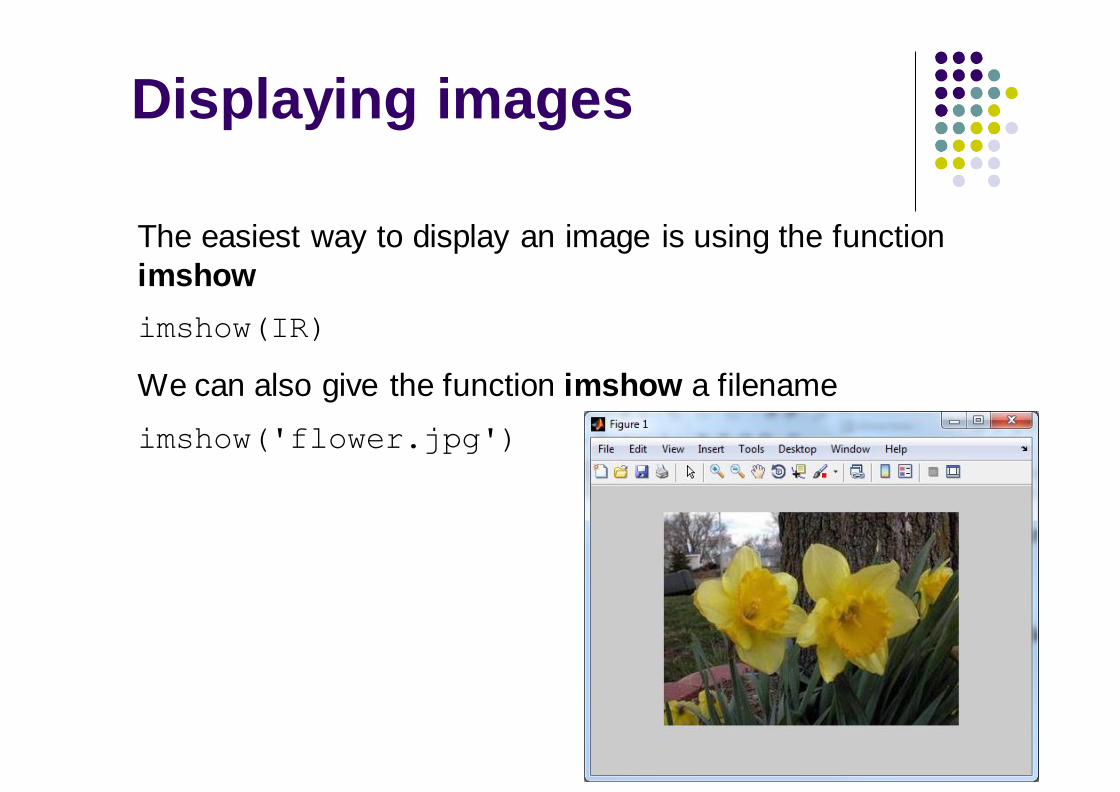
Displaying images

The easiest way to display an image is using the function

imshow

imshow(IR)

We can also give the function imshow a filename

imshow('flower.jpg')

Exercise

Load a TrueColor image from disk and save its three

components, RGB, separately into three images.

Example image: http://www.dsi.unive.it/~cosmo/material/matlab/flower.jpg

Image Type Conversion

Some algorithms need a specific image format.

We can convert images between different types: RGB,

Graysace, Binary.

RGB = imread('flower.jpg');

%Convert truecolor image to grayscale

GS = rgb2gray(RGB);

imwrite(GS,'flowergs.jpg');

Image Type Conversion

Convert a matrix to Grayscale Image using mat2gray.

The output is a double image with pixel intensity between 0

and 1.

M = magic(100);

%Convert truecolor image to grayscale

I = mat2gray(M);

imwrite(I,'magic1.jpg');

minv=0; maxv=(M(:))*2;

%Convert the matrix to gray image

%using the given bounds as values

%to rescale the input matrix

%I = (M-min)./(max-min)

I = mat2gray(M, [minv, maxv]);

imwrite(I,'magic2.jpg');

Image Type Conversion

I2 = im2double(I): convert a uint8 or uint16 image to

double image. I2 = im2uint8(I): convert image to uint8 image.

BW = im2bw(I, level) converts the input images in a

binary image (black and white). The level is a number

(threshold) between 0 and 1 which is used to decide

whether a pixel should assume the value 0 or 1.

level=0.3 level=0.5

Histogram plot

The command hist can be used to display the frequency

distribution of elements in a given vector.

hist(Y)bins the elements of Y in 10 equally spaced containers and display

a bar plot showing the number of elements in each bin.

%generate normally distributed pseudorandom vector

y = randn(10000,1);

%display the distribution histogram with 10 bins

hist(y)

%display the distribution histogram with 100 bins

hist(y,100)

%display the distribution histogram with

%lenght(vec) bins centered in the values of vec

vec=-6:0.05:6;

hist(y,vec)

Exercise

Download the TrueColor image from here

• Plot the RGB color histogram of the image (number of

pixel with a specific intensity value for each channel).

• Rescale the color values for each channel separately in

order to obtain an image similar to the original (here).

(r-minr)/(maxr-minr)

(g-ming)/(maxg-ming)

(b-minb)/(maxb-minb)

Exercise – Chroma Key

Download the image from here.

Produce a bitmap mask with ones on the portion of image

which belongs to the fuchsia strip of the controller.

You need to convert the image color space from RGB to YCbCr

(rgb2ycbcr) which is less sensible to changes in lighting.

http://en.wikipedia.org/wiki/YCbCr

Select only the pixels “near” the

target color in the YCbCr color space,

ignoring the luminance component.

B

R

G

Cb

Cr

y

Solution

function BW = yuvfilter(I,tolerance)

%YUVFILTER description….

yuv=rgb2ycbcr(im2double(I));

imgsize=size(I(:,:,1));

Cr = yuv(:,:,2);

Cb = yuv(:,:,3);

%Create the matrix of points in color space

CC = [Cr(:), Cb(:)];

%Compute the distabce from fuchsia (0.793,0.793);

CC = CC-0.793;

dist = sqrt(sum(CC.^2,2));

distI = reshape(dist, imgsize);

mask = im2bw(mat2gray(distI),tolerance);

imshow(mask);

end