handbook of nanophysics, k. sattler (ed.), taylor...

26-1

26.1 Introduction

The development of nanomaterials used in nanotechnology, for example, assembly of structures, manufacture of nanotubes, etc., requires the knowledge of mechanical properties such as Young’s modulus, the yield stress, or the buckling loadings. The evaluation by nanoindentation of these properties represents a real challenge for the researchers because it is difficult to carry out experiments at such length scales. Moreover, to validate an experimental result, it is necessary to be ensured of its reproducibility, which requires many samples and thus involves a high cost.

Recent developments in science and technology have advanced the capability to fabricate and control materials and devices with nanometer grain/feature sizes to achieve better mechani-cal properties in materials and more reliable performance in microelectromechanical systems (MEMS) and nanoelectrome-chanical systems (NEMS) (Bhushan, 1999; Miller and Tadmor, 2002; Vashishta et al., 2003; Tambe and Bhushan, 2004; Liu et al., 2005; Jian et al., 2006). Nanoindentation instrument provides a valid approach to investigate the mechanical characterizations of nanomaterials, such as the hardness, dislocation motion, and Young’s modulus, which are required to design structural/functional elements in micro- and nanoscale devices. Many powerful capabilities in in situ and ex situ imaging, acoustic emission detection, and high-temperature testing are now being used to probe nanoscale phenomena such as defect nucleation and dynamics, mechanical instabilities or strain localization, and phase transformations (Wang et al., 2003; Aouadia, 2006; Schuh, 2006; Gouldstone et al., 2007; Lin et al., 2007; Snyders et al., 2007; Szlufarska et al., 2007). With the same pace of experi-mental work, analytical theory and computer simulation, espe-cially the latter, are developed to reproduce or even predict the

intrinsic phenomena during nanoindentation (Vashishta et al., 2003; Szlufarska, 2006). Among these simulation methods, first principles calculations (FP) (Aouadia, 2006; Snyders et al., 2007), molecular dynamics (MD) (Noreyan et al., 2005; Liu et al., 2007), finite element method (FEM) (Liu et al., 2005; Feng et al., 2007; Zhong and Zhu, 2008), and their hybrid methods such as first principle molecular dynamics (FPMD) (Schneider et al., 2007) and quasicontinuum method (QC) (Miller and Tadmor, 2002; Dupuy et al., 2005), from the trade-off between efficiency and accuracy point of view, are mostly applied to investigate the evo-lution of structure and properties in different spatial and tempo-ral scales during nanoindentation.

We try to present in this chapter a review of the theoretical study and computational modeling of nanoindentation. The chap-ter is organized as follows. Section 26.2 is devoted to the basics of nanoindentation. Some classic solutions of indentation problems are summarized. In Section 26.3, solutions of contact and plas-ticity problems by the finite element method are presented with numerical examples. In Section 26.4, a survey on atomistic and multiscale approaches for nanoindentation modeling is provided.

The material of this chapter comes from the teaching notes and research works of the authors. We also used other research articles in the literature to supplement the content of various topics discussed in this chapter.

26.2 Principle and Methods of Nanoindentation

Nanoindentation is an important and popular mechanical experimental technique used in nanomaterials science and nan-otechnology. Compared with other mechanical experimental

26Theory of Nanoindentation

26.1 Introduction ...........................................................................................................................26-126.2 Principle and Methods of Nanoindentation ......................................................................26-126.3 Finite Element Analysis of Contact and Plasticity ...........................................................26-5

Modeling of Elastoplastic Materials at Finite Strains • Modeling of Contact Problems with Friction • Numerical Examples

26.4 Atomistic and Multiscale Approaches .............................................................................26-11First Principles Calculations for Nanoindentation Modeling • Molecular Dynamics Calculations for Nanoindentation Modeling • Multiscale Approaches for Nanoindentation Modeling

26.5 Conclusion and Perspective ...............................................................................................26-13References .........................................................................................................................................26-13

Zhi-Qiang FengUniversité d’Évry-Val d’Essonne

Qi-Chang HeUniversité Paris-Est

Qingfeng ZengNorthwestern Polytechnical University

Pierre JoliUniversité d’Évry-Val d’Essonne

75527_C026.indd 1 3/20/2010 2:48:58 AM

Handbook of Nanophysics, K. Sattler (ed.), Taylor & Francis, 2010

feng

Note

Marked définie par feng

26-2 Handbook of Nanophysics: Functional Nanomaterials

characterization methods, nanoindentation entails a quite sim-ple setup and specimen preparation. In addition, nanoindenta-tion leaves only a small imprint and can be thus considered as nondestructive. However, a correct and accurate exploitation of experimental data from nanoindentation tests necessitates a full understanding of the nanoindentation principle and of the assumptions made in carrying out nanoindentation tests. Since there exist a good few reviews on the experimental pro-cedure of nanoindentation and on the interpretation of nanoin-dentation test data (Bhushan, 2004; Cheng and Cheng, 2004; Fischer-Cripps, 2004, 2006; Sharpe, 2008), we focus on a clear presentation of the nanoindentation principle and a thorough discussion of the assumptions underlying nanoindentation tests.

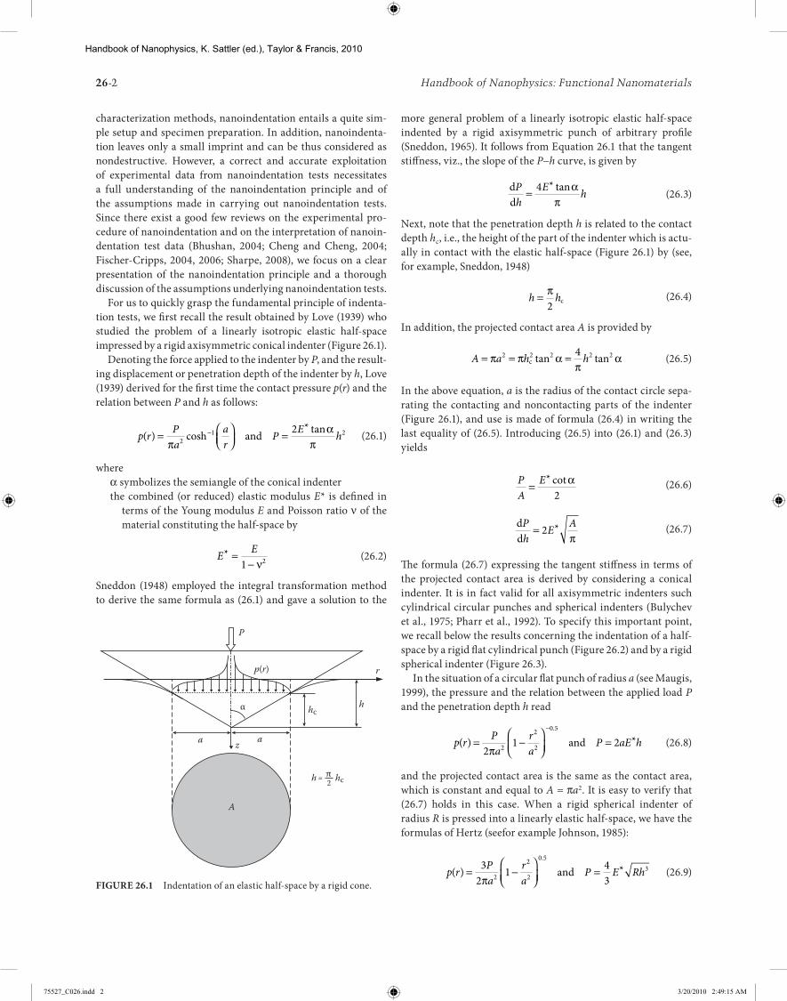
For us to quickly grasp the fundamental principle of indenta-tion tests, we first recall the result obtained by Love (1939) who studied the problem of a linearly isotropic elastic half-space impressed by a rigid axisymmetric conical indenter (Figure 26.1).

Denoting the force applied to the indenter by P, and the result-ing displacement or penetration depth of the indenter by h, Love (1939) derived for the first time the contact pressure p(r) and the relation between P and h as follows:

p r Pa

ar

P E h( ) cosh* tan=

=−

πα

π21 22and (26.1)

whereα symbolizes the semiangle of the conical indenterthe combined (or reduced) elastic modulus E* is defined in

terms of the Young modulus E and Poisson ratio ν of the material constituting the half-space by

E E* =−1 2ν

(26.2)

Sneddon (1948) employed the integral transformation method to derive the same formula as (26.1) and gave a solution to the

more general problem of a linearly isotropic elastic half-space indented by a rigid axisymmetric punch of arbitrary profile (Sneddon, 1965). It follows from Equation 26.1 that the tangent stiffness, viz., the slope of the P−h curve, is given by

ddPh

E h= 4 * tanαπ

(26.3)

Next, note that the penetration depth h is related to the contact depth hc, i.e., the height of the part of the indenter which is actu-ally in contact with the elastic half-space (Figure 26.1) by (see, for example, Sneddon, 1948)

h h= π2 c (26.4)

In addition, the projected contact area A is provided by

A a h h= = =π π απ

α2 2 2 2 24c tan tan (26.5)

In the above equation, a is the radius of the contact circle sepa-rating the contacting and noncontacting parts of the indenter (Figure 26.1), and use is made of formula (26.4) in writing the last equality of (26.5). Introducing (26.5) into (26.1) and (26.3) yields

PA

E=* cotα2

(26.6)

ddPh

E A= 2 *π

(26.7)

The formula (26.7) expressing the tangent stiffness in terms of the projected contact area is derived by considering a conical indenter. It is in fact valid for all axisymmetric indenters such cylindrical circular punches and spherical indenters (Bulychev et al., 1975; Pharr et al., 1992). To specify this important point, we recall below the results concerning the indentation of a half-space by a rigid flat cylindrical punch (Figure 26.2) and by a rigid spherical indenter (Figure 26.3).

In the situation of a circular flat punch of radius a (see Maugis, 1999), the pressure and the relation between the applied load P and the penetration depth h read

p r Pa

ra

P aE h( ) *.

= −

=−

21 22

2

2

0 5

πand (26.8)

and the projected contact area is the same as the contact area, which is constant and equal to A = πa2. It is easy to verify that (26.7) holds in this case. When a rigid spherical indenter of radius R is pressed into a linearly elastic half-space, we have the formulas of Hertz (seefor example Johnson, 1985):

p r Pa

ra

P E Rh( ) *.

= −

=32

1 432

2

2

0 53

πand (26.9)

a a

hch

h hcπ

r

α

P

p(r)

z

A

= 2

Figure 26.1 Indentation of an elastic half-space by a rigid cone.

75527_C026.indd 2 3/20/2010 2:49:15 AM


Theory of Nanoindentation 26-3

a Rh2 = (26.10)

where a is the radius of the circular contact surface. With (26.9) and (26.10), it is straightforward to check that (26.7) is satisfied.

Theoretically speaking, the reduced modulus E* of a linearly elastic isotropic solid would be easily identified by using (26.1) or (26.3) if the P−h curve could be experimentally determined for a rigid conical impressed into this solid. However, the experi-mental reality is much more complex, so that (26.1) cannot be directly applied. We now proceed to discuss the main aspects of real nanoindentation tests.

The indenter being most widely used for nanoindentation is not a conical one but the three-sided Berkovich indenter (Figure 26.4). The face semiangle θ of a typical Berkovich indenter is equal to 65.27°. The reason why the three-sided pyramidal Berkovich indenter is employed in nanoindentation rather than the more familiar four-sided Vickers one is that it is much easier to grind the three faces of the former than the four faces of the latter so as to meet at a point when both are made of diamond. Clearly, the geometry of the three-sided Berkovich indenter is quite different from that of a cone. Nevertheless, the forgoing results for a coni-cal indenter are in practice assumed to be applicable to a three-sided pyramidal indenter by requiring that these two indenters have the same ratio of the projected contact area A to the contact depth hc. More precisely, for the Berkovich indenter, the projected contact area is calculated in terms of the contact depth hc by

A h= 3 3 2 2c tan θ (26.11)

Setting A obtained by (26.11) to be equal to A given by (26.5) in terms of hc for θ = 65.27°, it follows that the semi-angle of the conical indenter “equivalent” to the Berkovich indenter is

α = °70 30. (26.12)

Introducing this value into (26.5) yields

A h h= =24 5 9 932 2. .c (26.13)

In nanoindentation, the indenter tip is usually made of dia-mond, which is strongly resistant to deformations but cannot be treated ultimately as rigid. In general, it is known from contact mechanics (Johnson, 1985) that when the indenter is deform-able, the reduced (or combined) elastic modulus E* involved in formula (26.1) should be defined by

1 1 12 2

E E Ei

i* = − + −ν ν (26.14)

A

a a

h

r

p(r)

P

z

Figure 26.2 Indentation of a half-space by a rigid circular flat punch.

a a

p(r)

P

h

r

z

A

Figure 26.3 Indentation of a half-space by a rigid spherical indenter.

60°60°

A

hc

θ

θ=65.27°

60°

Figure 26.4 Geometry of a three-sided Berkovich indenter.

75527_C026.indd 3 3/20/2010 2:49:24 AM



where Ei and νi are the Young’s modulus and Poisson ratio of the indenter. When the tip of an indenter consists of diamond, the values Ei = 1141 GPa and νi = 0.07 are commonly adopted.

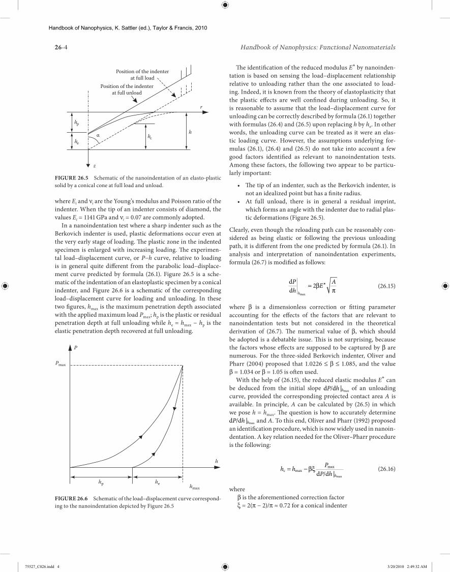
In a nanoindentation test where a sharp indenter such as the Berkovich indenter is used, plastic deformations occur even at the very early stage of loading. The plastic zone in the indented specimen is enlarged with increasing loading. The experimen-tal load–displacement curve, or P−h curve, relative to loading is in general quite different from the parabolic load–displace-ment curve predicted by formula (26.1). Figure 26.5 is a sche-matic of the indentation of an elastoplastic specimen by a conical indenter, and Figure 26.6 is a schematic of the corresponding load–displacement curve for loading and unloading. In these two figures, hmax is the maximum penetration depth associated with the applied maximum load Pmax; hp is the plastic or residual penetration depth at full unloading while he = hmax − hp is the elastic penetration depth recovered at full unloading.

The identification of the reduced modulus E* by nanoinden-tation is based on sensing the load–displacement relationship relative to unloading rather than the one associated to load-ing. Indeed, it is known from the theory of elastoplasticity that the plastic effects are well confined during unloading. So, it is reasonable to assume that the load–displacement curve for unloading can be correctly described by formula (26.1) together with formulas (26.4) and (26.5) upon replacing h by he. In other words, the unloading curve can be treated as it were an elas-tic loading curve. However, the assumptions underlying for-mulas (26.1), (26.4) and (26.5) do not take into account a few good factors identified as relevant to nanoindentation tests. Among these factors, the following two appear to be particu-larly important:

• The tip of an indenter, such as the Berkovich indenter, is not an idealized point but has a finite radius.

• At full unload, there is in general a residual imprint, which forms an angle with the indenter due to radial plas-tic deformations (Figure 26.5).

Clearly, even though the reloading path can be reasonably con-sidered as being elastic or following the previous unloading path, it is different from the one predicted by formula (26.1). In analysis and interpretation of nanoindentation experiments, formula (26.7) is modified as follows:

ddPh

E Ahmax

*= 2βπ

(26.15)

where β is a dimensionless correction or fitting parameter accounting for the effects of the factors that are relevant to nanoindentation tests but not considered in the theoretical derivation of (26.7). The numerical value of β, which should be adopted is a debatable issue. This is not surprising, because the factors whose effects are supposed to be captured by β are numerous. For the three-sided Berkovich indenter, Oliver and Pharr (2004) proposed that 1.0226 ≤ β ≤ 1.085, and the value β = 1.034 or β = 1.05 is often used.

With the help of (26.15), the reduced elastic modulus E* can be deduced from the initial slope d /dP h h| max of an unloading curve, provided the corresponding projected contact area A is available. In principle, A can be calculated by (26.5) in which we pose h = hmax. The question is how to accurately determine d /dP h h| max and A. To this end, Oliver and Pharr (1992) proposed an identification procedure, which is now widely used in nanoin-dentation. A key relation needed for the Oliver–Pharr procedure is the following:

h h PP h h

c d /d= −max

max

| max

βξ (26.16)

whereβ is the aforementioned correction factorξ = 2(π − 2)/π ≈ 0.72 for a conical indenter

Position of the indenterat full load

Position of the indenterat full unload

hp

α hch

r

z

he

Figure 26.5 Schematic of the nanoindentation of an elasto-plastic solid by a conical cone at full load and unload.

P

Pmax

hp he hmax

h

Figure 26.6 Schematic of the load–displacement curve correspond-ing to the nanoindentation depicted by Figure 26.5

75527_C026.indd 4 3/20/2010 2:49:32 AM



When setting β = 1, formula (26.16) can be rigorously deduced by combining (26.1), (26.3) and (26.4). In the Oliver–Pharr procedure, the load–displacement curve is first obtained by using a power-law function

P h h m= −η( )p (26.17)

to fit experimental data. In (26.17), m is the power-law index, η is a constant parameter, and hp is the residual penetration depth measured experimentally. With (26.17), it is easy to compute

dd pPh

m h hh

m

max

( )max= − −η 1 (26.18)

Substituting (26.18) and (26.16) into (26.5) gives the projected contact area A. Finally, the reduced modulus E* is calculated by (26.15).

Though becoming standard, the Oliver–Pharr procedure appears open to criticism with respect to the following two points. First, when the value of m is quite different from 2, the power law (26.17) used to fit experimental data may be incom-patible with formula (26.1), which is the starting point of the method on which the Oliver–Pharr procedure is based; even when m = 2, the identification of η by a fitting method implies the determination of E*. Second, the projected contact area A corresponding to the maximum load Pmax can be determined directly by formula (26.5) and via the measurement of hmax; the calculation of A by means of (26.16) is much more complicated, because the determination of the derivative d /dP h h| max is much more vulnerable to error than the measurement of hmax.

26.3 Finite Element Analysis of Contact and Plasticity

The analysis of nanoindentation can be very complex because of two principal strongly nonlinear phenomena:

• Elastic–plastic deformation of the indented materials• Frictional contact between the indenter and materials.

Different analytical models were proposed in the case of thin metal layers (with elastoplastic behavior) (Oliver and Pharr, 1992) or polymers (with hyperelastic behavior and pile-up) (Bucaille et al., 2003). In the case where analytical derivation of the mechanical properties is not feasible, numerical model-ing may therefore help to clarify and put in evidence the dif-ferent contributions of thin films and substrates. Knapp et al. (1999) used the finite element approach to determine hardness properties of thin films in two dimensions. They suggested a fit procedure to evaluate mechanical properties of thin layers and substrates. This kind of procedure reveals some success but with several limitations: two dimensional geometry, hundred of nanometers length scales, geometrically perfect indenter, and the neglecting of interface interactions (film/substrate). For smaller length scale, it seems to be necessary to develop more

complex interaction film-substrate models, as in the work of Bull et al. (Bull et al., 2004; Berasetgui et al., 2004) and Raabe et al. (Wang et al., 2004; Zaafarani et al., 2006).

The aim of this section is to describe the main numerical approaches in solving a three-dimensional elastoplastic contact problem.

26.3.1 Modeling of Elastoplastic Materials at Finite Strains

Usually, behavior laws of solids are differential equations that connect the rate of stress to the rate of strain. Nagtegaal (1982) and Hughes and Winget (1980) have proposed several integra-tion schemes. The concept of consistent linearization introduced by Nagtegaal (1982) and extended by Simo and Taylor (1985) made it possible to write, in the case of small or large deforma-tions, effective consistent tangent stiffness matrices.

At low temperature, or when the loading speeds are relatively low, the metallic materials present inelastic time-independent deformations. Within the framework of large deformation, the total rate of deformation tensor d is split into two components: an elastic part de, connected linearly to the Lie derivative of the Kirchhoff stress tensor τ, and a plastic part dp:

Lvt = = −D D: : ( )d d de p (26.19)

where 𝔻 denotes the fourth-order elasticity tensor.It is supposed that there exists a convex field (elastic domain)

in the space of stresses inside of which there is no plastic flow. The yield function f = 0 represents the loading surface delimiting the elastic domain. In the case of isotropic plasticity considered here, we use the von Mises criterion as follows:

f R R p( , , ) ( ) ( )τ τa h h a= − = −23

with dev (26.20)

where R(p) and 𝛂 represent, respectively, the radius and the cen-ter position of the elastic domain. dev(•) stands for the deviator tensor of (•) and h h h= : . In the case of associated plasticity, the normality rule is written by

d n np with= =�λ hh

(26.21)

where �l denotes the plastic multiplier. The plastic loading and unloading condition can be expressed in terms of the Kuhn–Tucker condition

� �λ λ≥ ≤ =0 0 0, ( , , ) , ( , , )f R f Rt a t a (26.22)

The isotropic law of strain hardening is defined by the evolution of the radius R with respect to the cumulated plastic strain p by

R p R R Rs sp( ) ( )= − − −

0 e γ (26.23)

75527_C026.indd 5 3/20/2010 2:49:48 AM



where Rs, R0, and γ are material constants. Rs represents the saturated radius of the elastic domain, and R0 the initial one as shown in Figure 26.7.

The rate of the cumulated plastic strain is given by

� �p p= =23

23

d λ (26.24)

The linear Prager kinematic hardening is defined by the evolu-tion of back stress 𝛂 of the elastic domain with respect to the plastic strain rate:

LvpHa = 2

3d (26.25)

where H is the slope of the kinematic work hardening. The iso-tropic strain hardening and the kinematic hardening can be respectively interpreted as the expansion and the translation of the elastic domain, as shown in Figure 26.8.

The integration of behavior laws plays a very important role in a finite element code. Indeed, it determines the precision of the solution. Errors on the estimates of the variables, once made, are not retrievable any more. Moreover when the estimates depend on the history of the loading, these errors can be propagated from an increment to another. The results deviate more and

more from the solution. In this study, the implicit integration algorithm has been chosen. Let us consider a plastically admissi-ble state (corresponding to the load step n) and the known char-acteristics of this state are: 𝛕n, 𝛂n, pn verifying f (𝛕n, 𝛂n, R(pn)) = 0. Integrating the behavior lows consists in finding the characteris-tics of the state n + 1. The most used method to integrate the laws of plastic behavior is undoubtedly the “radial return mapping” (RRM), initially introduced by Wilkins (1964), Krieg and Krieg (1977) for models of perfectly plastic behavior. The extension of this method to the case of the models with nonlinear kinematic work hardening was carried out by Simo and Taylor (1986). The principle of this method is to calculate the final stress 𝛕n+1 as the projection of a test stress 𝛕E onto the yield surface according to the normal passing by 𝛕E (Figure 26.8). The test stress is calcu-lated by supposing that the increment of strain is entirely elastic. A standard stress update is outlined at following (for details, see Simo and Hughes, 1998, Chapter 8).

Say the position vectors in the “deformed” and “undeformed” state are represented by x and X respectively and the displace-ment vector u = x − X, the total deformation gradient is defined as

F xX

I u= ∂∂

= + ∇ (26.26)

One of the major challenges while integrating the rate con-stitutive equations at finite strains is to achieve incremental objectivity. To this end, it is common to define an intermediate configuration between load steps, n and n + 1:

x x x F F Fn n n n n n+ + + += − + = − +

∈

θ θθ θ θ θ

θ

( ) ( )

[ , ]

1 1

0 1

1 1and

with (26.27)

The relative deformation gradients fn+θ and f~

n+θ, the relative incremental displacement gradient hn+θ and the incremental Eulerian strain tensor e~n+θ are defined by

f F F f f f h u xx

e

n n n n n n nn

n

n

+ +−

+ + +−

++

+

+

= = = ∂∂

=

θ θ θ θ θθ

θ

θ

11

1

12

, , ( ) ,�

� �� f I f f fnT

n nT

n+ + +−

+− θ θ( )1 11

(26.28)

Within the interval [tn, tn+1], the deformation gradient can be expressed as

d h h h hn n nT

nT

nt+ + + + += + + − θ θ θ θ θθ12

1 2∆

( ) (26.29)

The objective approximation for the Lie derivative of the Kirchhoff stress is given by

Lv n n n n nT

n nT

tτ θ θ θ+ + +

−+ +

−+= −

11

11 1∆

f f f ft t (26.30)

By evaluating (26.19) at the intermediate configuration and using the flow rule (26.21), we obtain

R(p)

p

Rs

R0

Loading Unloading

Figure 26.7 Loading and unloading.

gn+1=0

gn=0

xn

nn

Rn+1

Rn

σ3Δx

σn

σ1 σ2

σn+1

σE

Figure 26.8 Radial return mapping.

75527_C026.indd 6 3/20/2010 2:50:04 AM



∆ ∆ ∆ ∆ ∆t t tv n n n nL t + + + += − =θ θ θ θλ λ λD : [ ]d n with � (26.31)

Similarly, we have

a an n n nT

nH+ + + += +θ θ θ θλf f n23

∆ (26.32)

Table 26.1 summarizes the predictor–corrector step in the RRM integration algorithm developed above.

26.3.2 Modeling of Contact Problems with Friction

The analysis of contact problems with friction is of great impor-tance in many engineering applications (Johnson, 1985). The numerical treatment of the unilateral contact with dry friction is certainly one of the nonsmooth mechanics topics for which many efforts have been made in the past. In the literature, many approaches have been developed to deal with such prob-lems using the finite element method. A large literature base is available for a variety of numerical algorithms (Zhong, 1993; Wriggers, 2002). The bipotential method proposed by DeSaxcé and Feng (1998) has been successfully applied to solve contact problems between elastic or hyperelastic bodies (Feng et al., 2005, 2006). In the present work, this method will be applied to solve the nanoindentation problem involving the contact between the rigid indenter and the elastoplastic film.

26.3.2.1 Governing Equations

The finite element method is often used in computational mechanics. Without going into details, quasistatic nonlinear behaviors of solid media, discretized by Ne finite elements, are governed by the following equilibrium equations:

F F R 0in ex− − = (26.33)

whereFex denotes the vector of external loadsr is the vector of contact reaction forces

The vector of internal forces Fin is calculated by

F F F Bin in inwith d= ∧ == ∫e

Ne e T

V

e

e

V1

s (26.34)

The symbol ∧ denotes a standard finite element assembly opera-tor. The Cauchy stress tensor 𝛔 is related to the Kirchhoff stress tensor 𝛕 by 𝛔 = 𝛕/det(F) and the latter is obtained from the inte-gration of the constitutive laws as shown in Section 26.3.1. It is noted that Equation 26.33 is strongly nonlinear with respect to the nodal displacements u, because of finite strains and large displacements of solid. Moreover, the constitutive laws of con-tact with friction are usually represented by inequalities and the contact potential is even nondifferentiable. A typical solu-tion procedure for this type of nonlinear analysis is obtained by using the Newton–Raphson iterative procedure (Joli and Feng, 2008):

K U F R F

U U U

Ti i i i

i i i

∆

∆

= + −

= ++

ex in

1 (26.35)

where i and i + 1 are the iteration numbers at which the equa-tions are computed. KT = ∂Fin/∂u stands for the tangent stiffness matrix and Δu the vector of nodal displacements correction.

It is noted that Equation 26.35 cannot be solved directly because Δu and r are both unknown. The key idea is to deter-mine first the reaction vector r in a reduced system which only concerns the contact nodes. Then, the displacement increments can be computed in the whole structure using contact reactions as external loading. In the following, we focus our attention on describing how to determine the contact forces. Let us begin with the general description of contact kinematics.

26.3.2.2 Contact Kinematics

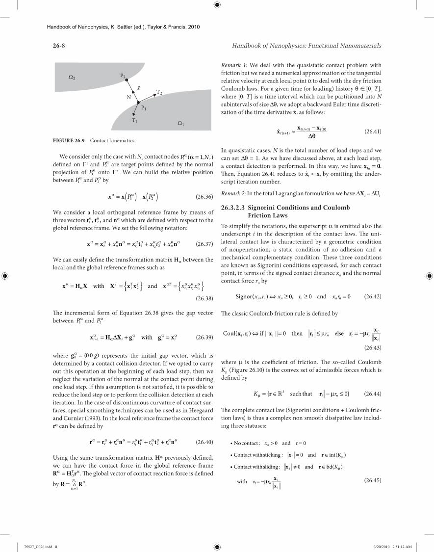
First of all, basic definitions and notations used are described. For the sake of simplicity, we consider two deformable bodies Ωa (Figure 26.9), a = 1, 2, coming into contact. Each body is decom-posed by finite elements and the nodal positions in the global coordinate frame are represented by the vector xa. The boundary Γa of each body is assumed to be sufficiently smooth everywhere such that an outward unit normal vector can be defined at any point Pa on Γa.

Table 26.1 Radial Return Mapping Algorithm1. Elastic predictor

t t a a

h

nE

n n nT

n nE

n n nT

nE

n nEp p

+ + + + + + +

+ +

= + =

= =

θ θ θ θ θ θ θ

θ θ

f f e f fD : ;

;

�

ddev t a hh

nE

nE

nnE

nE+ + ++

+( ) − =θ θ θ

θ

θ

; n

2. Plastic corrector

f R p

f

nE

nE

nE

n

nE

+ + +

+

+

= − ( )<

=

θ θ θ

θ

θ

h 23

0if then

set

E

( ) ( )• •

else

∆

∆

λ θ µ

µ

θ µ λ θ

θ

= +

+ + ′ ′ =

+ = + − +

+ = +

fnE

H R R Rp

n n n

n n

2

13

1 2

1

with dd

E

E

t t

a a

n

++ +

+ = + +

23

123

∆

∆

λ θ

θ λ

H n

pn pn

n

E

75527_C026.indd 7 3/20/2010 2:50:23 AM



We consider only the case with Nc contact nodes P N1 cα α( , )= 1

defined on Γ1 and P2α are target points defined by the normal

projection of P1α onto Γ2. We can build the relative position

between P1α and P2

α by

x x xα α α= ( ) − ( )P P1 2 (26.36)

We consider a local orthogonal reference frame by means of three vectors t1

α, t2α , and nα which are defined with respect to the

global reference frame. We set the following notation:

x x n t nα α α α α α α α α α= + = + +t n t t nx x x t x1 21 2 (26.37)

We can easily define the transformation matrix Hα between the local and the global reference frames such as

x H X X x x xα

αα α α α= = { } = { }with andT T T T

t t tx x x n1 2 1 2 (26.38)

The incremental form of Equation 26.38 gives the gap vector between P1

α and P2α

x H X g g xi i i i i+ = + =1α

αα α α∆ with (26.39)

where g0 0 0α = ( )g represents the initial gap vector, which is determined by a contact collision detector. If we opted to carry out this operation at the beginning of each load step, then we neglect the variation of the normal at the contact point during one load step. If this assumption is not satisfied, it is possible to reduce the load step or to perform the collision detection at each iteration. In the case of discontinuous curvature of contact sur-faces, special smoothing techniques can be used as in Heegaard and Curnier (1993). In the local reference frame the contact force rα can be defined by

r r n t t nα α α α α α α α α α= + = + +t n t t nr r r r1 21 2 (26.40)

Using the same transformation matrix Hα previously defined, we can have the contact force in the global reference frame R H rα

αα= T . The global vector of contact reaction force is defined

by r r= ∧=α

α

1

Nc .

Remark 1: We deal with the quasistatic contact problem with friction but we need a numerical approximation of the tangential relative velocity at each local point α to deal with the dry friction Coulomb laws. For a given time (or loading) history θ ∈ [0, T], where [0, T] is a time interval which can be partitioned into N subintervals of size Δθ, we adopt a backward Euler time discreti-zation of the time derivative x. t as follows:

�x x xt i

t i t( )

( ) ( )+

+≈ −1

1 0

∆θ (26.41)

In quasistatic cases, N is the total number of load steps and we can set Δθ = 1. As we have discussed above, at each load step, a contact detection is performed. In this way, we have x 0t0 = . Then, Equation 26.41 reduces to x. t ≈ xt by omitting the under-script iteration number.

Remark 2: In the total Lagrangian formulation we have ΔXi = Δui.

26.3.2.3 Signorini Conditions and Coulomb Friction Laws

To simplify the notations, the superscript α is omitted also the underscript i in the description of the contact laws. The uni-lateral contact law is characterized by a geometric condition of nonpenetration, a static condition of no-adhesion and a mechanical complementary condition. These three conditions are known as Signorini conditions expressed, for each contact point, in terms of the signed contact distance xn and the normal contact force rn by

Signor and( , ) ,x r x r x rn n n n n n⇔ ≥ ≥ =0 0 0 (26.42)

The classic Coulomb friction rule is defined by

Coul if then else( , )x r x r r x

xt t t t n t nt

tr r⇔ = ≤ = −� � 0 µ µ

(26.43)

where μ is the coefficient of friction. The so-called Coulomb Kμ (Figure 26.10) is the convex set of admissible forces which is defined by

K rt nµ µ= ∈ − ≤{ }r r�3 0such that (26.44)

The complete contact law (Signorini conditions + Coulomb fric-tion laws) is thus a complex non smooth dissipative law includ-ing three statuses:

i

i

Nocontact and

Contact withsticking and

:

: int( )

x

K

n

t

> =

= ∈

0 0

0

r

x r µ

ii Contact withsliding and bd

with

: ( )x r

r xx

t

t nt

t

K

r

≠ ∈

= −

0 µ

µ

(26.45)

Ω2

Ω1

P2

T2

T1

P1

N

g

Figure 26.9 Contact kinematics.

75527_C026.indd 8 3/20/2010 2:51:12 AM



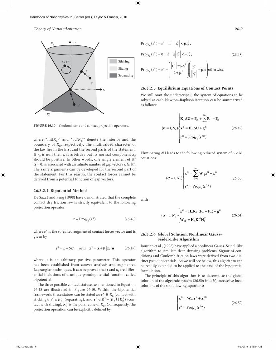
where “int(Kμ)” and “bd(Kμ)” denote the interior and the boundary of Kμ, respectively. The multivalued character of the law lies in the first and the second parts of the statement. If rn is null then x is arbitrary but its normal component xn should be positive. In other words, one single element of ℝ3 (r = 0) is associated with an infinite number of gap vectors x ∈ ℝ3. The same arguments can be developed for the second part of the statement. For this reason, the contact forces cannot be derived from a potential function of gap vectors.

26.3.2.4 Bipotential Method

De Saxcé and Feng (1998) have demonstrated that the complete contact dry friction law is strictly equivalent to the following projection operator:

r rK= Proj µ ( *) (26.46)

where r* is the so-called augmented contact forces vector and is given by

r r x x x x n* * *= − = +ρ µwith t (26.47)

where ρ is an arbitrary positive parameter. This operator has been established from convex analysis and augmented Lagrangian techniques. It can be proved that r and xt are differ-ential inclusions of a unique pseudopotential function called bipotential.

The three possible contact statuses as mentioned in Equation 26.45 are illustrated in Figure 26.10. Within the bipotential framework, these statues can be stated as: r* ∈ Kμ (contact with sticking), r* *∈Kµ (separating), and r* ( *)∈ −� ∪3 K Kµ µ (con-tact with sliding). Kµ* is the polar cone of Kμ. Consequently, the projection operation can be explicitly defined by

Proj if

Proj if

Proj

K t n

K t n

K

r

r

µ

µ

µ

µ

µ

( *) * * *,

( *) * *,

( *)

r r r

r r

r

= <

= < −0

== −−

+

−

r

r rr

n** * *

*.

t nt

t

rµ

µµ

1 2 otherwise

(26.48)

26.3.2.5 Equilibrium Equations of Contact Points

We still omit the underscript i, the system of equations to be solved at each Newton–Raphson iteration can be summarized as follows:

( , )

( * )

α

α

α

αα

α

α αµ

=

= + ∧ −

= +

=

=

1

1

N

T

N

c

ex in

c

Proj

K U F R

x H U g

r r

∆

∆

F

K

(26.49)

Eliminating Δu leads to the following reduced system of 6 × Nc equations:

( , )

( * )

α

ααβ

β α

β

α αµ

== +

=

=∑

1 1N

Nc

c

Proj

x W r x

r r

�

K

(26.50)

with

( , )( )

αα

αα

αβ α β

== − +

=

−

−1

1

1N

T

T

cex in

T

�x H K F F g

W H K H

(26.51)

26.3.2.6 Global Solution: Nonlinear Gauss–Seidel-Like Algorithm

Jourdan et al., (1998) have applied a nonlinear Gauss–Seidel-like algorithm to simulate deep drawing problems. Signorini con-ditions and Coulomb friction laws were derived from two dis-tinct pseudopotentials. As we will see below, this algorithm can be readily extended to be applied to the case of the bipotential formulation.

The principle of this algorithm is to decompose the global solution of the algebraic system (26.50) into Nc successive local solutions of the six following equations:

x W r x

r rK

ααα

α αβ

α αµ

= +

=

Proj ( * )

(26.52)

Kμ

Kμ*

rn

rt

r= r*

r*

r*

r

Sticking

Separating

Sliding

Figure 26.10 Coulomb cone and contact projection operators.

75527_C026.indd 9 3/20/2010 2:51:34 AM



with

x W r xαβ

αββ α

β β α

= += ≠∑ �1,

Nc

(26.53)

where xαβ represents the part of the relative position at the contact point α due to the initial gap, the external forces, and contact forces of Nc − 1 other contact nodes β. This contribution is “frozen” during each local solution. One series of Nc local solutions corresponds to one iteration k of the algorithm. The iterative process is successively applied for each contact point (α = 1, Nc) until the convergence of the solution. The contact convergence criterion is stated as

r

r

( ) ( )

( )

k k

k g

+

+

−≤

1

1

rε

(26.54)

wherer r r r= { }1 2� Nc is the vector of contact reactions of all contact

nodesεg is a user-defined tolerance. The initial condition is given

by r(0) = 0

In the bipotential formulation, the usual approach to solve the local implicit equations (26.52) is to use a predictor/corrector Uzawa algorithm. Many examples have been successfully treated by Feng et al. (Feng, 1995; Feng et al., 2003).

26.3.2.7 Local Solution: Uzawa Algorithm

The numerical solution of the implicit equation (26.52) can be carried out by means of the Uzawa algorithm, which leads thus to an iterative process involving one predictor–corrector step:

Predictor

Corrector

r r x x n

r

α α αβ αβ

α

ρ µ*( ) ( ) ( ) ( ) ( )

(

k k k kt

k+ = − +( )1

kk k+ +=1 1) ( )( * )ProjK rµα

(26.55)

where k and k + 1 are the iteration numbers at which the contact reactions are computed. The corrector step is explicitly given by Equation 26.48. In view of Equation 26.52, the gap vector is updated by

x W r xααα

α αβ( ) ( ) ( )k k k+ += +1 1 (26.56)

It is noted that the solution is controlled by a global convergence criterion (iteration k) as stated in Equation 26.54. The advan-tage of this approach is the simplicity of programming and the numerical robustness but it needs more iterations when com-pared with the implicit Newton algorithm presented recently in (Joli and Feng, 2008). However, the latter is more time-consum-ing at each iteration.

26.3.3 Numerical Examples

26.3.3.1 Boussinesq–Love Indentation Problem

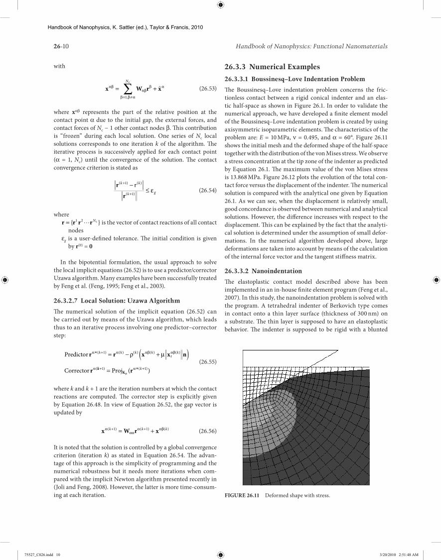
The Boussinesq–Love indentation problem concerns the fric-tionless contact between a rigid conical indenter and an elas-tic half-space as shown in Figure 26.1. In order to validate the numerical approach, we have developed a finite element model of the Boussinesq–Love indentation problem is created by using axisymmetric isoparametric elements. The characteristics of the problem are: E = 10 MPa, ν = 0.495, and α = 60°. Figure 26.11 shows the initial mesh and the deformed shape of the half-space together with the distribution of the von Mises stress. We observe a stress concentration at the tip zone of the indenter as predicted by Equation 26.1. The maximum value of the von Mises stress is 13.868 MPa. Figure 26.12 plots the evolution of the total con-tact force versus the displacement of the indenter. The numerical solution is compared with the analytical one given by Equation 26.1. As we can see, when the displacement is relatively small, good concordance is observed between numerical and analytical solutions. However, the difference increases with respect to the displacement. This can be explained by the fact that the analyti-cal solution is determined under the assumption of small defor-mations. In the numerical algorithm developed above, large deformations are taken into account by means of the calculation of the internal force vector and the tangent stiffness matrix.

26.3.3.2 Nanoindentation

The elastoplastic contact model described above has been implemented in an in-house finite element program (Feng et al., 2007). In this study, the nanoindentation problem is solved with the program. A tetrahedral indenter of Berkovich type comes in contact onto a thin layer surface (thickness of 300 nm) on a substrate. The thin layer is supposed to have an elastoplastic behavior. The indenter is supposed to be rigid with a blunted

Figure 26.11 Deformed shape with stress.

75527_C026.indd 10 3/20/2010 2:51:48 AM



point of radius of curvature of approximately 50 nm. Figure 26.13 shows the model with a grid in 3D as well as a more detailed view in 2D. It should be noted that the symmetry of the model is taken into account in order to reduce the computing time. As discussed in Section 26.2, we needed to have a triangu-lar base pyramid with the tip rounded. The tip of the indenter has been created with a 3D animation program (LightWave 7.5). It has several special features that have allowed us to realize the rounded tip with a radius of 50 nm with a tolerance of 2% as shown in Figure 26.13. Then we have applied a mesh on this 3D object. The mesh of the film and the substrate are generated with an appropriate level of meshing to have the minimum number of contact elements between the tip and our meshed material, as we can see in Figure 26.13.

Figure 26.14 shows the print left on the surface and the distri-bution of stresses around the zone of indentation. The triangu-lar form of the print accurately reproduces what we observe in experiments on this scale.

Recently, a micro/nanoscale computational contact model is proposed in (Sauer and Li, 2007) to study the adhesive contact between deformable bodies.

26.4 Atomistic and Multiscale Approaches

The basic concept of modeling of natural phenomena is based on computing the energy of a physical structure, since both the static and dynamic properties of the structure are related with the first or higher order derivative of energy with respect to structure positions and time. People always try to predict prop-erties of materials with the aid of as few experimental data as possible. Generally, the fewer the experimental data are input, the higher the computational resources cost. Some atomistic calculations ask for powerful supercomputers or clusters with thousands of CPUs but still cover a structure size around 100 nm (Vashishta et al., 2003). Consequently, multiscale approaches are required for practical nanoindentation modeling.

26.4.1 First Principles Calculations for Nanoindentation Modeling

First principles calculations use the laws of quantum mechanics based solely on a small number of physical constants, the speed of light, Planck’s constant, the masses and charges of electrons and nuclei, to obtain the energy by solving the Schrödinger equation (Leach, 2001):

− ∇ +

= ∂∂

hm

t ih tt

2

22

8 2π πV r rΨ Ψ( , ) ( , ) (26.57)

hereΨ is the wave functionr the position of the particlet the timeh the Planck’s constantm the mass of the particle∇2 the Laplacian operatorV the potential field in which the particle is movingi the imaginary unit

BoussinesqNumerical

400

350

300

250

200

150

100

50

00 1 2 3

Displacement (mm)

Forc

e (N

)

4 5

Figure 26.12 Load–displacement curve.

Figure 26.13 3D and 2D view of the mesh.

Figure 26.14 Numerical and experimental results.

75527_C026.indd 11 3/20/2010 2:51:52 AM



Exact solutions to the equation are not trivial, so a variety of mathematical transformation and approximation techniques are proposed. Born–Oppenheimer approximation separates nuclear and electronic motions. Nonrelativistic approximation treats the mass of the particles independent of their speeds. The orbital approximation makes the total wave function of the many-particle system constructable from one-electron wave functions. The nonrelativistic, time-independent form of the Schrödinger description is as follows:

H EΨ Ψ( ) ( )r r= (26.58)

whereE is the energy of the systemH the Hamiltonian operator, equal to

H h

mii

= − ∇ +∑2

22

8πV

(26.59)

The resistance of a material to deformations is related to its elastic constants. The linear elastic constants form a 6 × 6 sym-metric matrix, three tensile and three shear components, having 21 different components, such that σi = Dijεj for stresses, σ, and strains, ε. Consequently, elastic constants can be evaluated by calculating the stress tensor for a number of slightly distorted structures. In this case, the internal coordinates are optimized by minimizing the total energy in each run, while keeping the lattice parameters fixed. Strains can be applied in the x, y, or z directions or shear strains can be applied. Other properties such as the bulk modulus (response to an isotropic compression), Poisson coefficient, Lame constants, and so forth can be com-puted from the values of Dij.

26.4.2 Molecular Dynamics Calculations for Nanoindentation Modeling

Molecular dynamics (MD) simulation studies were initiated in the late 1950s at the Lawrence Radiation Laboratory (LRL) by Alder and Wainwright (Alder and Wain-wright, 1959, 1960) in the field of equilibrium and nonequilibrium statistical mechan-ics. The key idea of the molecular dynamic model is quite simple and it consists in computing trajectories of a finite set of atoms from numerical integration of equations of motion. We present here the basic principle of molecular dynamic by considering a triangular network in which atoms are connected by interaction forces derived from potential functions (harmonic or Lennard-Jones). The scenario of the simulation consists in applying stress σ or velocity v conditions onto the boundary of the network (Figure 26.15).

For each atom of position xi, we establish the dynamic equa-tions following the second Newton law. Only the contributions of the external forces due to the potential interaction of the j connected atom and the local damping force are taken into account as follows:

mi i ij i

j

�� x F x= −∑ η

(26.60)

where mi and η are respectively the mass and the damping parameter of the atom i. The interaction force between two atoms is defined by

F x x

x xiji j

i jg d=

−−

( )

(26.61)

This force can be differentiated from potential functions giving several mathematical formulations of g(d), such as

Harmonic potential: ( ) ( )g d k d a= − − (26.62)

Lennard Jones potential: ( )g d ka a

dad

=

−

6

13 7

(26.63)

where a and d represent respectively the resting length and the distance during the simulation between two atoms in interac-tion. The parameter k denotes the stiffness between two atoms. Zhang et al. has used the Lennard-Jones potential function for numerical simulation of mechanical behaviors of carbon nano-tubes (Zhang et al., 2007).

Classically, the ordinary differential equations (26.60) are integrated by using an explicit numerical scheme such as the Verlet numerical scheme (Verlet, 1967). The time step of the numerical integration is constant and to prevent any prob-lem of numerical instability, it must be very small as compared to the lowest characteristic period of the physical system.

In the simulation of nanoindentation, the load on the indenter P can be calculated by summing the forces acting on the atoms of the indenter in the indentation direction. Indentation depth h can be calculated as the displacement of the tip of the indenter relative to the initial surface of the indented solid (Szlufarska, 2006). The coordinates and velocities at a later time can be

–v d

i

j–σ

v

σ

Figure 26.15 Network of atoms.

75527_C026.indd 12 3/20/2010 2:52:06 AM



determined, once the initial coordinates and velocities of the atoms are known. A load–displacement (P−h) response and the deformation structures in a material can be analyzed by moni-toring the trajectories of the atoms.

Since most of the empirical potentials for MD calculations need the comparison with experimental data, this limits the application for new materials or for materials where experimen-tal data do not exist. Another drawback of MD is that there is no universal force field can be applied to an atom in different chemical environment. For example, potentials of carbon in dia-mond and C60 have different values and/or forms (Brenner, 1990; Smith and Beardmore, 1996; Christopher et al., 2001).

26.4.3 Multiscale Approaches for Nanoindentation Modeling

Because discrete atomic effects become important only in the vicinity of defects, interfaces and surfaces, multiscale approaches aim to model an atomistic system without explicitly treating every atom in the problem (Miller and Tadmor, 2002; Zeng et al., 2009). There are mainly two types of multiscale methods (Liu et al., 2004): concurrent and hierarchical. Concurrent methods, such as quasicontinuum (QC) method (Miller and Tadmor, 2002), simul-taneously solve a fine-scale model in some local region of inter-est and a coarser scale model in the remainder of the domain. Hierarchical, or serial coupling methods, such as heterogenous multiscale method (HMM) (Weinan et al., 2003), use results of a fine-scale model simulation to acquire data for a coarser-scale model that is used globally, e.g., to determine parameters for constitutive equations. Currently, both quantum mechanics and empirical interatomic potentials are using to describe the atomic details depends on the nature of practical problems and the com-putation cost (Abraham et al., 1998; Ogata et al., 2001).

In the case of concurrent methods, lots of efforts have been made to solve the “pad” or “handshake” region between the coarse and fine scales. A bridging domain method was proposed in Xiao and Belytschko (2004) for coupling continua with molecu-lar dynamics. The purpose of the handshake region is to assure smoother coupling between the atomistic and continuum regions. These methods were reviewed and further improved in (Karpov et al., 2006). In the case of hierarchical methods, scale separation is exploited so that coarse-grained variables can be evolved on macroscopic spatial/temporal scales using data that are predicted based on the simulation of the microscopic process on microscale spatial/temporal domains (Weinan et al., 2003). As for a real appli-cation, concurrent and hierarchical methods can be combined to yield optimal efficiency.

26.5 Conclusion and Perspective

Nanoindentation becomes more and more important because of the development of nanomaterials and MEMS/NEMS. Modeling and simulation are good approaches to “look at” the details during the deformation of a material or devices under external forces.

We have presented in this chapter a review of the principle and methods of nanoindentation. Two principal nonlinear problems presented in nanoindentation (contact and plasticity) are solved by means of the finite element method with effective algorithms. The state of the art on atomistic and multiscale approaches for nanoindentation modeling is presented and discussed.

It seems that the theoretical models could be extended to take into account the friction and the numerical models could be improved by considering the adhesion in the uni-lateral contact model. To identify the properties of materials, an optimization procedure could be carried out to minimize the difference between the experimental P − h curve and the numerical one.

With the development of realistic computational models, efficient algorithms and powerful computer resources, multi-scale phenomena of nanoindentation can be easily understood by freely adjusting parameters beyond the scope of laboratory experiments. This information is of importance to design high quality and multifunctional MEMS/NEMS, and more generally, in nanoscience and nanotechnology.

References

Abraham, F. F., Broughton, J. Q., Bernstein, N., and Kaxiras, E. (1998). Spanning the length scales in dynamic simulation. Comput. Phys., 12(6), 538–546.

Alder, B., and Wainwright, T. (1959). Studies in molecular dynam-ics: I. General method. J. Chem. Phys., 31, 459.

Alder, B. and Wainwright, T. (1960). Studies in molecular dynam-ics: II. Behavior of a small number of elastic spheres. J. Chem. Phys., 33, 1439.

Aouadia, S. M. (2006). Structural and mechanical properties of TaZrN films: Experimental and ab initio studies. J. Appl. Phys., 99, 053507.

Berasetgui, E. G., Bull, S. J., and Page, T. F. (2004). Mechanical modelling of multilayer optical coatings. Thin Solid Films, 447–448, 26–32.

Bhushan, B. (1999). Nanoscale tribophysics and tribomechanics. Wear, 225–229, 465–492.

Bhushan, B. (2004). (ed.) Springer Handbook of Nanotechnology, 2nd edition. Berlin, Germany: Springer.

Brenner, D. (1990). Empirical potential for hydrocarbons for use in simulating the chemical vapor deposition of diamond films. Phys. Rev. B, 42, 9458.

Bucaille, J. L., Stauss, S., Felder, E., and Michler, J. (2003). Determination of plastic properties of metals by instru-mented indentation using different sharp indenters. Acta Mater., 51, 1663–1678.

Bull, S. J., Berasetgui, E. G., and Page, T. F. (2004). Modelling of the indentation response of coatings and surface treat-ments. Wear, 256, 857–866.

Bulychev, S. I., Alekhin, V. P., Shorshorov, M. K., Ternovskii, A. P., and Shnyrev, G. D. (1975). Determining Young’s modu-lus from the indenter penetration diagram. Zavodskaya Laboratoriya, 41, 1137–1140.

75527_C026.indd 13 3/20/2010 2:52:06 AM



Cheng, Y. T., and Cheng, C. M. (2004). Scaling dimensional analysis and indentation measurements. Mater. Sci. Eng. R, 44, 91–149.

Christopher, D., Smith, R., and Richter, A. (2001). Nanoindentation of carbon materials. Nucl. Instrum. Meth. Phys. Res. B, 180, 117–124.

DeSaxcé, G. and Feng, Z.-Q. (1998). The bi-potential method: A constructive approach to design the complete contact law with friction and improved numerical algorithms. Math. Comput. Model., 28(4–8), 225–245.

Dupuy, L. M., Tadmor, E. B., Miller, R. E., and Phillips, R. (2005). Finite-temperature quasicontinuum: Molecular dynamics without all the atoms. Phys. Rev. Lett., 95, 060202.

Feng, Z.-Q. (1995). 2D or 3D frictional contact algorithms and applications in a large deformation context. Commun. Numer. Meth. Eng., 11, 409–416.

Feng, Z.-Q., Peyraut, F., and Labed, N. (2003). Solution of large deformation contact problems with friction between Blatz-Ko hyperelastic bodies. Int. J. Eng. Sci., 41, 2213–2225.

Feng, Z.-Q., Joli, P., Cros, J.-M., and Magnain, B. (2005). The bi-potential method applied to the modeling of dynamic prob-lems with friction. Comput. Mech., 36, 375–383.

Feng, Z.-Q., Peyraut, F., and He, Q.-C. (2006). Finite deforma-tions of Ogden’s materials under impact loading. Int. J. Non-Linear Mech., 41, 575–585.

Feng, Z.-Q., Zei, M., and Joli, P. (2007). An elasto-plastic contact model applied to nanoindentation. Comput. Mater. Sci., 38, 807–813.

Fischer-Cripps, A. C. (2004). Nanoindentation. Berlin, Germany: Springer.

Fischer-Cripps, A. C. (2006). Critical review and interpretation of nanoindentation test data. Surf. Coat. Technol., 200, 4153–4165.

Gouldstone, A., Chollacoop, N., Dao, M., Li, J., Minor, A. M., and L., S. Y. (2007). Indentation across size scales and disci-plines: Recent developments in experimentation and mod-eling. Acta Mater., 55, 4015–4039.

Heegaard, J. H. and Curnier, A. (1993). An augmented Lagrangian method for discrete large slip contact problems. Int. J. Numer. Meth. Eng., 36, 569–593.

Hughes, T. J. L. and Winget, J. (1980). Some computational aspects of elastic-plastic large strain analysis. Int. J. Numer. Meth. Eng., 15, 1862–1867.

Jian, S. R., Fang, T. H., Chuu, D. S., and Ji, L. W. (2006). Atomistic modeling of dislocation activity in nanoindented GaAs. Appl. Surf. Sci., 253, 833–840.

Johnson, K. L. (1985). Contact Mechanics. Cambridge, U.K.: Cambridge University Press.

Joli, P. and Feng, Z.-Q. (2008). Uzawa and Newton algorithms to solve frictional contact problems within the bi-potential framework. Int. J. Numer. Meth. Eng., 73, 317–330.

Jourdan, F., Alart, P., and Jean, M. (1998). A Gauss-Seidel like algorithm to solve frictional contact problems. Comput. Meth. Appl. Mech. Eng., 155, 31–47.

Karpov, E. G., Yu, H., Park, H. S., Liu, W. K., Wang, Q. J., and Qian, D. (2006). Multiscale boundary conditions in crys-talline solids: Theory and application to nanoindentation. Int. J. Solids Struct., 43, 6359–6379.

Knapp, J. A., Follstaedt, D. M., Myers, S. M., Barbour, J. C., and Friedmann, T. A. (1999). Finite-element modeling of nanoindentation. J. Appl. Phys., 58, 1460–1474.

Krieg, R. D., and Krieg, B. D. (1977). Accuracies of numerical solution method for the elastic-perfectly plastic model. ASME, J. Pres. Vess. Pip. Div., 99, 510–515.

Leach, A. R. (2001). Molecular Modelling: Principles and Applications. Englewood Cliffs, NJ: Prentice-Hall.

Liu, C. L., Fang, T. H., and Lin, J. F. (2007). Atomistic simulations of hard and soft films under nanoindentation. Mater. Sci. Eng., A 452–453, 135–141.

Liu, W. K., Karpov, E. G., Zhang, S., and Park, H. S. (2004). An introduction to computational nanomechanics and materi-als. Comput. Meth. Appl. Mech. Eng., 193, 1529–1578.

Liu, Y., Wang, B., Yoshino, M., Roy, S., Lu, H., and Komanduri, R. (2005). Combined numerical simulation and nanoin-dentation for determining mechanical properties of sin-gle crystal copper at mesoscale. J. Mech. Phys. Solids, 53, 2718–2741.

Liu, Y. H., Chen, T. C., Yang, P. F., Jian, S. R., and Lai, Y. S. (2007). Atomic-level simulations of nanoindentation-induced phase transformation in mono-crystalline silicon. Appl. Surf. Sci., 254, 1415–1422.

Love, A. E. H. (1939). Boussinesq’s problem for a rigid cone. Quart. J. Math., 10, 161.

Maugis, D. (1999). Contact, Adhesion and Rupture of Elastic Solids. Berlin, Germany: Springer.

Miller, R. E. and Tadmor, E. B. (2002). The quasicontinuum method: Overview, applications and current directions. J. Comput.-Aided Mater. Des., 9, 203–239.

Nagtegaal, J. C. (1982). On the implementation of inelastic consti-tutive equations with special reference to large deformation problems. Comput. Meth. Appl. Mech. Eng., 33, 469–484.

Noreyan, A., Amar, J. G., and Marinescua, I. (2005). Molecular dynamics simulations of nanoindentation of beta-SiC with diamond indenter. Mater. Sci. Eng., B 117, 235–240.

Ogata, S., Lidorikis, E., Shimojo, F., Nakano, A., Vashishta, P., and Kalia, R. (2001). Hybrid Finite-element/Molecular-dynamics/Electronic-density-functional approach to mate-rials simulations on parallel computers. Comput. Phys. Commun., 138, 143–154.

Oliver, W. C. and Pharr, G. M. (1992). An improved technique for determining hardness and elastic modulus using load and displacement sensing indentation experiments. J. Mater. Res., 7, 1564–1583.

Oliver, W. C. and Pharr, G. M. (2004). Measurement of hardness and elastic modulus by instrumented indentation: Advances in understanding and refinements to methodology. J. Mater. Res., 19, 3–20.

75527_C026.indd 14 3/20/2010 2:52:06 AM



Pharr, G. M., Oliver, W. C., and Brotzen, F. R. (1992). On the gen-erality of the relationship among contact stiffness, contact area and the elastic modulus during indentation. J. Mater. Res., 7, 613–617.

Sauer, R. A., and Li, S. (2007). An atomic interaction-based con-tinuum model for adhesive contact mechanics. Finite Elem. Anal. Des., 43, 384–396.

Schneider, J. M., Sigumonrong, D. P., Music, D., Walter, C., Emmerlich, J., Iskandar, R., et al. (2007). Elastic properties of Cr2AlC thin films probed by nanoindentation and ab ini-tio molecular dynamics. Scripta Mater., 57, 1137–1140.

Schuh, C. A. (2006). Nanoindentation studies of materials. Mater. Today, 9, 32–40.

Sharpe, W. N. (2008). Springer Handbook of Experimental Solid Mechanics. Berlin, Germany: Springer.

Simo, J. C. and Hughes, T. J. R. (1998). Computational Inelasticity. New York: Springer-Verlag.

Simo, J. C. and Taylor, R. L. (1985). Consistent tangent operator for rate-independent elasto-plasticity. ASME, J. Pres. Vess. Pip. Div., 48, 101–118.

Simo, J. C. and Taylor, R. L. (1986). A return mapping algorithm for plane stress elastoplasticity. Int. J. Numer. Meth. Eng., 22, 649–670.

Smith, R., and Beardmore, K. (1996). Molecular dynamics simu-lations of particle impacts with carbon-based materials. Thin Solid Films, 272, 255–270.

Sneddon, I. N. (1948). Boussinesq’s problem for a rigid cone. Mathematical Proceedings of the Cambridge Philosophical Society, 44, 492–507.

Sneddon, I. N. (1965). The relation between load and penetra-tion in the axisymmetric Boussinesq problem for a punch of arbitrary profile. Int. J. Eng. Sci., 3, 47–57.

Snyders, R., Music, D., Sigumonrong, D., Schelnberger, B., Jensen, J., and Schneider, J. M. (2007). Experimental and ab initio study of the mechanical properties of hydroxyapatite. Appl. Phys. Lett., 90, 193902.

Szlufarska, I. (2006). Atomistic simulations of nanoindentation. Mater. Today, 9(5), 42–50.

Szlufarska, I., Kalia, R. K., Nakano, A., and Vashishta, P. (2007). A molecular dynamics study of nanoindentation of amor-phous silicon carbide. J. Appl. Phys., 102, 023509.

Tambe, N. S. and Bhushan, B. (2004). Scale dependence of micro/nano-friction and adhesion of MEMS/NEMS materials, coatings and lubricants. Nanotechnology, 15, 1561–1570.

Vashishta, P., Kalia, R. K., and Nakano, A. (2003). Multimillion atom molecular dynamics simulations of nanostructures on parallel computers. J. Nanoparticle Res., 5, 119–135.

Verlet, L. (1967). Computer experiments on classical fluids, I: Thermodynamical properties of Lennard-Jones molecules. Phys. Rev., 159, 98–103.

Wang, W., Jiang, C. B., and Lu, K. (2003). Deformation behav-ior of Ni3Al single crystals during nanoindentation. Acta Mater., 51, 6169–6180.

Wang, Y., Raabe, D., Klüber, C., and Roters, F. (2004). Orientation dependence of nanoindentation pile-up patterns and of nanoindentation microtextures in copper single crystals. Acta Mater., 52, 2229–2238.

Weinan, E., Engquist, B., and Huang, Z. (2003). Heterogeneous multi-scale method - a general methodology for multi-scale modeling. Phys. Rev. B, 67 (9), 092101.

Wilkins, M. L. (1964). Calculation of elastic-plastic flow. In Methods of Computational Physics, B. Alder, S. Fernbach and M. Retenberg (Eds.), New York: Academic press, 3:211–263.

Wriggers, P. (2002). Computational Contact Mechanics. Chichester, U.K.: John Wiley & Sons.

Xiao, S. P., and Belytschko, T. (2004). A bridging domain method for coupling continua with molecular dynamics. Comput. Meth. Appl. Mech. Eng., 193, 1645–1669.

Zaafarani, N., Raabe, D., Singh, R. N., Roters, F., and Zaefferer, S. (2006). Three-dimensional investigation of the texture and microstructure below a nanoindent in a Cu single crystal using 3D EBSD and crystal plasticity finite element simula-tions. Acta Mater., 54, 1863–1876.

Zeng, Q., Zhang, L., Xu, Y., Cheng, L., and Yan, X. (2009). A uni-fied view of materials design: Two-element principle. Mater. Des., 30, 487–493.

Zhang, H. W., Wang, J. B., Ye, H. F., and Wang, L. (2007). Parametric variational principle and quadratic program-ming method for van der Waals force simulation of parallel and cross nanotubes. Int. J. Solids Struct., 44, 2783–2801.

Zhong, Y., and Zhu, T. (2008). Simulating nanoindentation and predicting dislocation nucleation using interatomic poten-tial finite element method. Comput. Meth. Appl. Mech. Eng., 197, 3174–3181.

Zhong, Z. H. (1993). Finite Element Procedures for Contact-Impact Problems. Oxford, NY: Oxford University Press.

75527_C026.indd 15 3/20/2010 2:52:06 AM


handbook of nanophysics, k. sattler (ed.), taylor...

Documents