hadoop programming
TRANSCRIPT

Introduction to Distributed Computing
Introduction to Hadoop
Mani [email protected] Thursday, Nov 01, 2012
About this course ¨ About large data processing ¨ Focus on problem solving ¨ Map Reduce and Hadoop ¨ HBase ¨ Hive ¨ Less on Administration ¨ More on Programming
In pioneer days they used oxen for heavy pulling, and when one ox couldn’t budge a log, they didn’t try to grow a larger ox. We shouldn’t be trying for bigger and bigger computer, but for more systems of computers.
- Grace Hopper
Session 1 - Introduction ¨ Introduction ¨ ○ Distributed computing ¨ ○ Parallel computing ¨ ○ Concurrency ¨ ○ Cloud Computing ¨ ○ Data Past, Present and Future ¨ ○ Computing Past, Present and Future ¨ ○ Hadoop ¨ ○ NoSQL
What is Hadoop ¨ Framework written in Java
¤ Designed to solve problem that involve analyzing large data (Petabyte)
¤ Programming model based on Google’s Map Reduce
¤ Infrastructure based on Google’s Big Data and Distributed File System
¤ Has functional programming roots (Haskell, Erlang, etc.,)
¤ Remember how merge sort work and try to apply the logic to large data problems
What is Hadoop ¨ Hadoop is an open source framework for writing and running distributed applications
that process large amounts of data. ¨ Hadoop Includes
¤ Hadoop Common utilities. ¤ Avro: A data serialization system with scripting languages. ¤ Chukwa: managing large distributed systems. ¤ HBase: A scalable, distributed database for large tables. ¤ HDFS: A distributed file system. ¤ Hive: data summarization and ad hoc querying. ¤ Map Reduce: distributed processing on compute clusters. ¤ Pig: A high-level data-flow language for parallel computation. ¤ Zookeeper: coordination service for distributed applications.
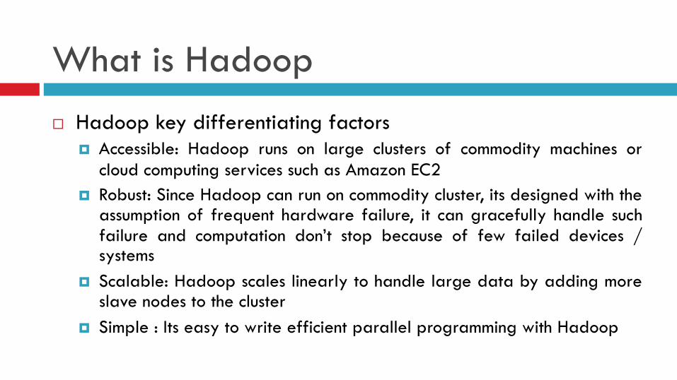
What is Hadoop ¨ Hadoop key differentiating factors
¤ Accessible: Hadoop runs on large clusters of commodity machines or cloud computing services such as Amazon EC2
¤ Robust: Since Hadoop can run on commodity cluster, its designed with the assumption of frequent hardware failure, it can gracefully handle such failure and computation don’t stop because of few failed devices / systems
¤ Scalable: Hadoop scales linearly to handle large data by adding more slave nodes to the cluster
¤ Simple : Its easy to write efficient parallel programming with Hadoop
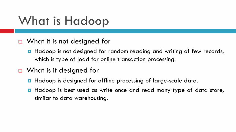
What is Hadoop ¨ What it is not designed for
¤ Hadoop is not designed for random reading and writing of few records, which is type of load for online transaction processing.
¨ What is it designed for ¤ Hadoop is designed for offline processing of large-scale data. ¤ Hadoop is best used as write once and read many type of data store,
similar to data warehousing.
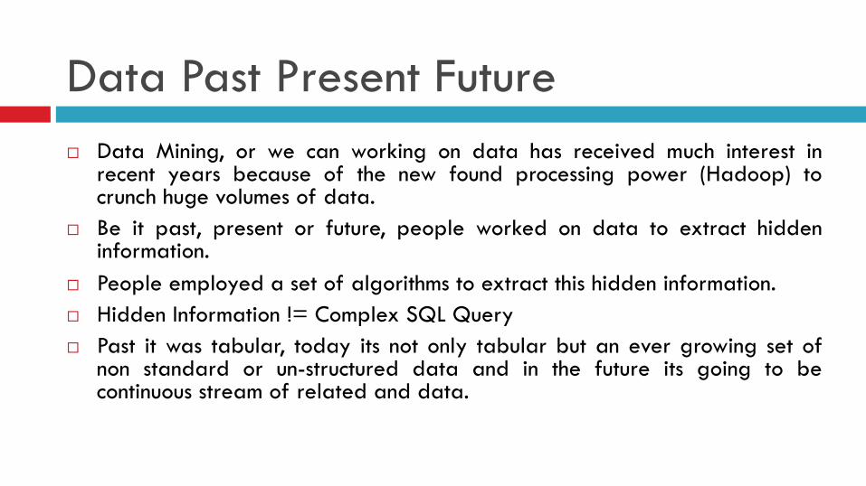
Data Past Present Future ¨ Data Mining, or we can working on data has received much interest in
recent years because of the new found processing power (Hadoop) to crunch huge volumes of data.
¨ Be it past, present or future, people worked on data to extract hidden information.
¨ People employed a set of algorithms to extract this hidden information. ¨ Hidden Information != Complex SQL Query ¨ Past it was tabular, today its not only tabular but an ever growing set of
non standard or un-structured data and in the future its going to be continuous stream of related and data.
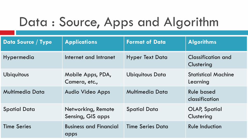
Data : Source, Apps and Algorithm Data Source / Type Applications Format of Data Algorithms
Hypermedia Internet and Intranet Hyper Text Data Classification and Clustering
Ubiquitous Mobile Apps, PDA, Camera, etc.,
Ubiquitous Data Statistical Machine Learning
Multimedia Data Audio Video Apps Multimedia Data Rule based classification
Spatial Data Networking, Remote Sensing, GIS apps
Spatial Data OLAP, Spatial Clustering
Time Series Business and Financial apps
Time Series Data Rule Induction
Role of Functional Programming
¨ Non Mutating ¨ No Side Effects ¨ Testability & Debugging ¨ Concurrency
Case Study : Google Search
¨ Crawling and storing data ¨ Building Inverted Index ¨ Searching ¨ Analytics ¨ Advertising
Case Study : PayPal
¤ Customer Sentiment Analysis ¤ Fraud Detection ¤ Market Segmentation ¤ Large dataset and complex data model with a need to
process at high frequency ¤ Manage data store across geographical and having
the capability to read and write them from anywhere.
Session 2 - Understanding Hadoop Stack
¨ Understanding Hadoop Stack ¨ ○ MapReduce ¨ ○ NoSQL ¨ ○ CAP Theorem ¨ ○ Databases: Key Value, Document, Graph ¨ ○ HBase and Cassandra ¨ ○ Hive and Pig ¨ ○ HDFS
What is Map Reduce ¨ A programming model designed by Google, using
which a sub set of distributed computing problems can be solved by writing simple programs.
¨ It provides automatic data distribution and aggregation.
¨ Removes problems with parallel programming, it believes in shared nothing architecture.
¨ To Scale, systems should be stateless.
Map Reduce ¨ A simple and powerful interface that enables automatic
parallelization and distribution of large-scale computations, combined with an implementation of this interface that achieves high performance on large clusters of commodity PCs
¨ Partitions input data ¨ Schedules execution across a set of machines ¨ Handles machine failure ¨ Manages inter-process communication
Recap Hadoop ¨ Hadoop is a framework for solving large scale distributed application, it
provides a reliable shared storage and analysis system.
¨ The storage is provided by Hadoop Distributed File System and analysis provided by Map Reduce, both are implementation of Google Distributed File System (Big Table) and Google Map Reduce.
¨ Hadoop is designed for handling large volume of data using commodity hardware and can process those large volume of data.
Understanding MapReduce
¨ Programming model based on simple concepts ¤ Iteration over inputs ¤ Computation of Key Value Pair from each piece of
input ¤ Grouping of intermediate value by key ¤ Iteration over resulting group ¤ Reduction of each group
HDFS Basic Features ¨ The Hadoop Distributed File System (HDFS) is a distributed
file system designed to run on commodity hardware ¨ Highly fault-tolerant and is designed to be deployed on
low-cost hardware ¨ Provides high throughput access to application data and is
suitable for applications that have large data sets ¨ Can be built out of commodity hardware
HDFS Design Principle - Failure ¨ Failure is the norm rather than exception ¨ A HDFS instance may consist of thousands of server
machines, each storing part of the file system’s data. ¨ At any point in time there is a high probability that few
components are non-functional (due to the high probability of system failure).
¨ Detection of faults and quickly recovering from them in an automated manner is the core architectural goal of HDFS.
HDFS Architecture ¨ Master / Slave Architecture
¨ HDFS cluster consist of a single NameNode, this manages the file system namespace and regulates access to files by clients
¨ Many Data Nodes, typically one DataNode for a physical node
¨ DataNode manages storage attached to the node in which they run.
¨ HDFS exposes a file system namespace and allows user data to be stored in files.
¨ File is split into one or more blocks and set of such blocks are stored in each DataNode
¨ The NameNode executes file system namespace operations like opening, closing, and renaming files and directories
¨ NameNode determines the mapping of blocks to DataNodes
¨ DataNode serves read, write, perform block operation, delete, and replication upon request from NameNode
¨ The existence of a single NameNode in a cluster greatly simplifies the architecture of the system. The NameNode is the arbitrator and repository for all HDFS metadata. The system is designed in such a way that user data never flows through the NameNode.
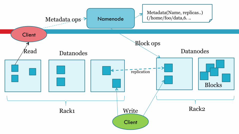
Namenode
B replication
Rack1 Rack2
Client
Blocks
Datanodes Datanodes
Client
Write
Read
Metadata ops Metadata(Name, replicas..) (/home/foo/data,6. ..
Block ops
Session 3 – Hadoop HandOn
Session 4 - MapReduce Introduction ¨ Functional - Concept of Map ¨ Functional - Concept of Reduce ¨ Functional - Ordering, Concurrency, No Lock, Concurrency ¨ Functional - Shuffling ¨ Functional - Reducing, Key, Concurrency ¨ MapReduce Execution framework ¨ MapReduce Partitioners and Combiners ¨ MapReduce and role of distributed filesystem ¨ Role of Key and Pairs ¨ Hadoop Data Types
Map Reduce – Introduction ¨ Divide and conquer is the only feasible way to solve large scale
data problems. ¨ Basic idea is to partition a large problem into smaller problems, to
the extend that the sub problems are independent, they can be tackled in parallel by different worker. Intermediate results from workers are combined to produce the final result.
¨ This general principle behind divide and conquer is broadly applicable to a wide range of problems, the impeding factor is in the details of implementation.
Map Reduce – Introduction ¨ Issues in Divide & Conquer
¤ How do we break a large problem into smaller tasks? How do we decompose the problem so that smaller task can be executed in parallel?
¤ How do we assign task to workers distributed across a potentially a large number of machines? ¤ How do we ensure workers get the data they need? ¤ How do we coordinate synchronization among different workers? ¤ How do we share partial result from one worker that is needed another? ¤ How do we accomplish all of the above in the face of software error and hardware failure? In traditional parallel programming, the developer needs to explicitly address many of the issues.
Map Reduce – Introduction ¨ Map Reduce are executed in two main phases, called
mapping and reducing. ¨ Each phase is defined by a data processing function
and these functions are called mapper and reducer. ¨ In map phase , MR takes the input data and feeds each
data element into mapper. ¨ The Reducer process all output from mapper and
arrives at final output.
Map Reduce – Introduction
¨ In order for mapping, reducing, partitioning, and shuffling to seamlessly work together, we need to agree on a common structure for data being processed.
¨ It should be flexible and powerful enough to handle most of the target data processing application.
¨ Map Reduce use list and pair<key,value> as its fundamental primitive data structure.
Functional Programming ¨ Functional Programming treats computation as evaluation of
function and it avoids mutation. ¨ a = a + 1 does not make sense in functional programming,
they make sense only in imperative programming. ¨ Functional programming emphasis is more on application of
function to members of list where as imperative programming is more about change in state and mutation.
Functional vs. Imperative ¨ Imperative programming lack referential transparency, that is, a
function or piece of code would produce different results depending on when the function was called and it depends on the state of the program.
¨ Functional programming does not lack referential transparency, that is, the output of the function depends only on the argument.
¨ In functional programming the functions are idempotent in nature, that is, calling the function on the data multiple times produces the same result.
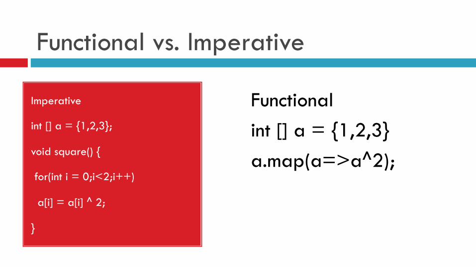
Functional vs. Imperative
Imperative
int [] a = {1,2,3};
void square() {
for(int i = 0;i<2;i++)
a[i] = a[i] ^ 2;
}
Functional int [] a = {1,2,3} a.map(a=>a^2);
Functional vs. Imperative
¨ Imperative programming are mutating in nature, that is, they modify the state of the program / data so calling a function twice might not give the same result as the program might have changed the state.
¨ Functional programming are immutable in nature, that is, no state are changed, calling a function multiple time does produce same result every time.

Map Reduce and Functional ¨ We now know that Map Reduce programs can process huge volume of data and to do that it
runs on large number of clusters. ¨ In examples we have seen so far, we have not seen any example where some state has to be
changed or state change has to notified, the map and reduce were applying function on data and not mutating.
¨ The question might arise, if not mutating, what are we doing, what happens when a map function executes a logic over data. We get a new List as a result of map function.
n Example: List<Integer> data; n data.map(data => data^2) n The map produces another List<Integer> called some tempDataList, but doing this the original list is not
corrupted. n Calling map function again produces the same result, this is the property based on which map reduce is
implemented.
Map Reduce – Processing List ¨ Map reduce can be looked as some list processing
framework that happens in a distributed environment. ¨ In Map Reduce, a list of input data is transformed in to list of
output data, the original input data is not modified, a new list is created that contains the transformed list.
¨ Have a look into merge sort algorithm, especially the merge portion of the algorithm to see how similar is that to map reduce.
Mapping
¨ This is probably the first step that Map Reduce starts with (apart from reading input files, configuration, etc)
¨ The map is provided with a list as input, the FileInputFormater takes care of providing this list.
¨ Inside the map, each element in the list is transformed and made available for next level.
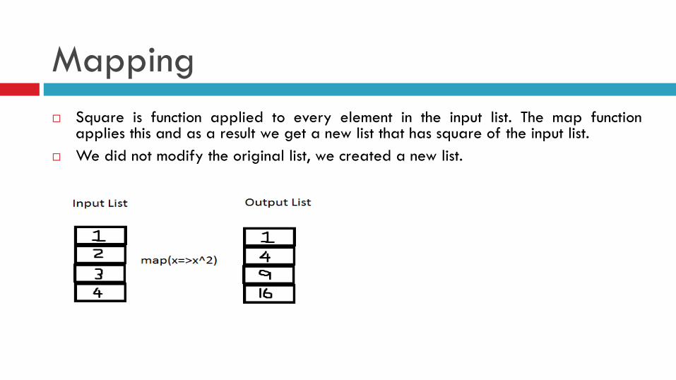
Mapping ¨ Square is function applied to every element in the input list. The map function
applies this and as a result we get a new list that has square of the input list. ¨ We did not modify the original list, we created a new list.
Reducer
¨ The next task done by map reduce is reducer ( for now forget the intermediate shuffle and sort)
¨ Each reducer gets a key and a list of values for the key.
¨ The reducer job is transform / reduce those list of values into a single value.
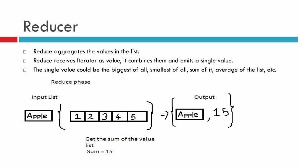
Reducer ¨ Reduce aggregates the values in the list. ¨ Reduce receives Iterator as value, it combines them and emits a single value. ¨ The single value could be the biggest of all, smallest of all, sum of it, average of the list, etc.
Map and Reduce Phase
¨ Map is Parallel in nature, each element in the list is processed independently. ¤ That is, key and values are scattered in the document space,
each map job might look at some portion of data and find the key and its values, like this many map works in parallel.
¨ Reduce is sequential in nature, that is all values of the key are processed one after another.
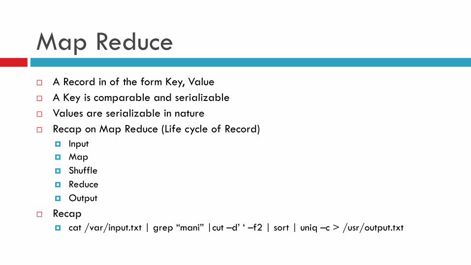
Map Reduce ¨ A Record in of the form Key, Value ¨ A Key is comparable and serializable ¨ Values are serializable in nature ¨ Recap on Map Reduce (Life cycle of Record)
¤ Input ¤ Map ¤ Shuffle ¤ Reduce ¤ Output
¨ Recap ¤ cat /var/input.txt | grep “mani” |cut –d’ ‘ –f2 | sort | uniq –c > /usr/output.txt
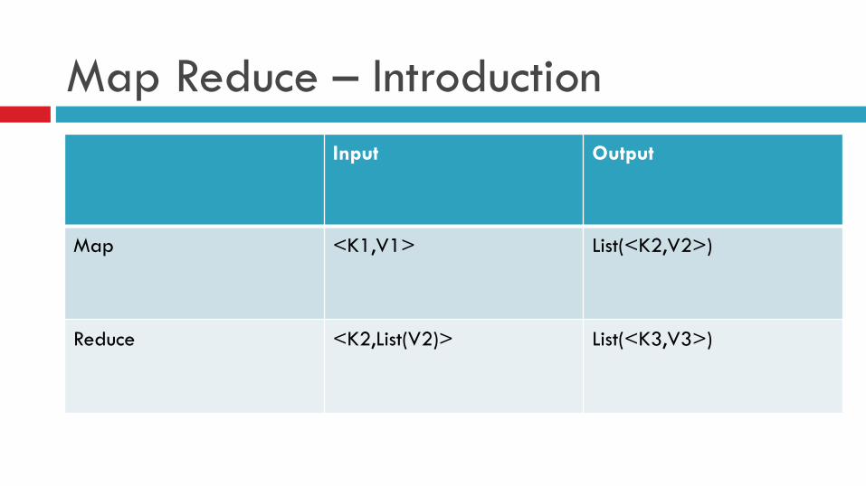
Map Reduce – Introduction Input Output
Map <K1,V1> List(<K2,V2>)
Reduce <K2,List(V2)> List(<K3,V3>)
Map Reduce - Introduction
¨ Map ¤ Records from the data source ( line output of files, rows
of database, etc) are fed into the map function as <key, value> pairs, e.g (filename, line).
¤ Map() function produces one or more intermediate values along with an output keys from the input.
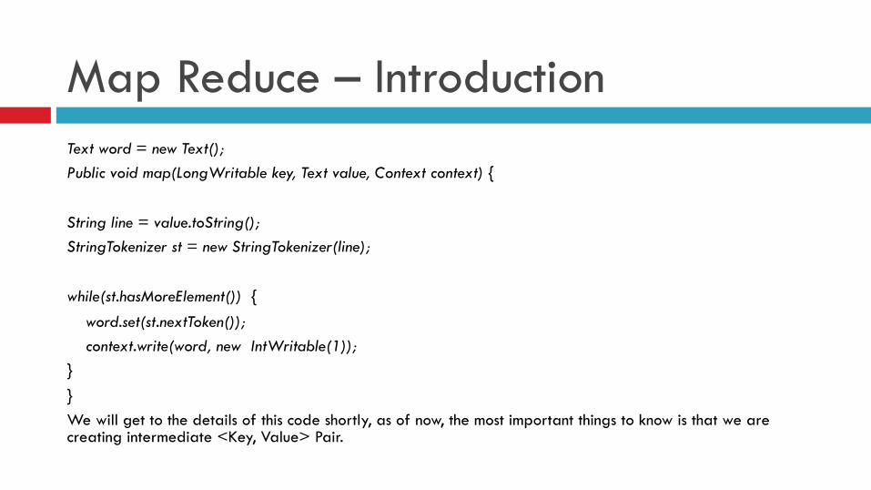
Map Reduce – Introduction Text word = new Text(); Public void map(LongWritable key, Text value, Context context) {
String line = value.toString(); StringTokenizer st = new StringTokenizer(line);
while(st.hasMoreElement()) {
word.set(st.nextToken()); context.write(word, new IntWritable(1)); }
} We will get to the details of this code shortly, as of now, the most important things to know is that we are creating intermediate <Key, Value> Pair.
Map Reduce - Introduction
¨ Reduce ¤ After map phase is over, all intermediate values of a
given output key are combined together into a list. ¤ Reduce combine these intermediate values into one or
more final values for the same output key.

Map Reduce - Introduction Public void reduce(Text key, Iterator<IntWritable> values, Context context) {
Int sum = 0;
while( values.hasNext() )
sum += values.next().get(); // ! = count , it’s the value in the list
context.write(key, new IntWritable(sum));
}
Map Reduce - Introduction
¨ Parallelism – Joining the dots ¤ Map function runs in parallel, creating different
intermediate values from different input data sets. ¤ Reduce function also runs in parallel, each working on a
different output key. ¤ All values are processed independently.
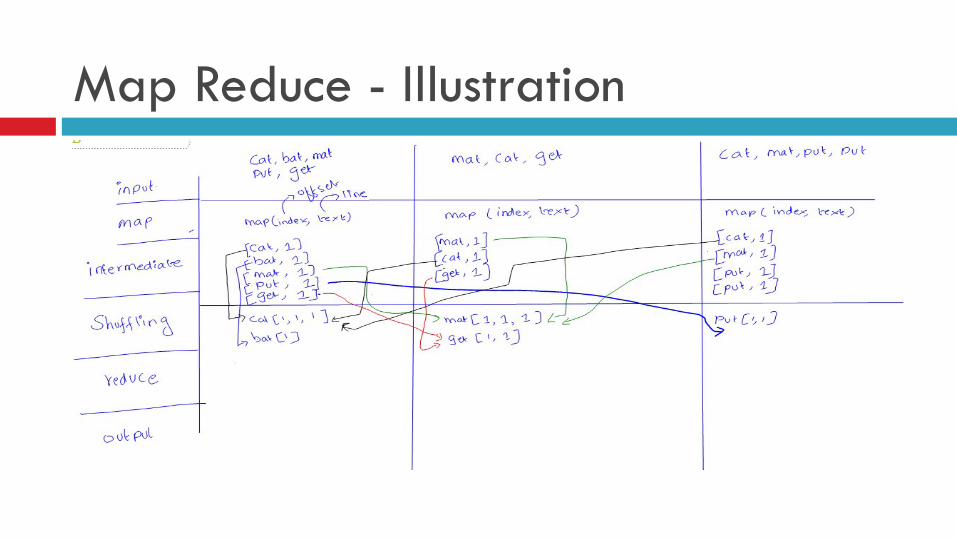
Map Reduce - Illustration
Map Reduce - Introduction
¨ We don’t have to bother about sorting. ¨ We don’t have to bother about shuffling. ¨ We don’t have to bother about communication and
scheduling. ¨ All we have to bother and care is about data and
task.
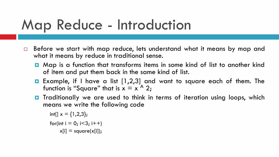
Map Reduce - Introduction ¨ Before we start with map reduce, lets understand what it means by map and
what it means by reduce in traditional sense. ¤ Map is a function that transforms items in some kind of list to another kind
of item and put them back in the same kind of list. ¤ Example, if I have a list [1,2,3] and want to square each of them. The
function is “Square” that is x = x ^ 2; ¤ Traditionally we are used to think in terms of iteration using loops, which
means we write the following code int[] x = {1,2,3};
for(int i = 0; i<3; i++) x[i] = square(x[i]);
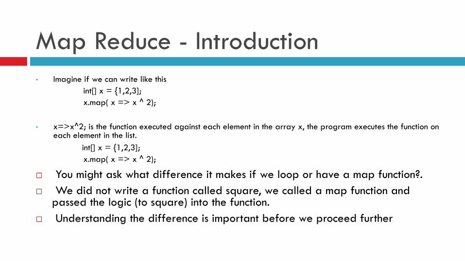
Map Reduce - Introduction • Imagine if we can write like this
int[] x = {1,2,3]; x.map( x => x ^ 2);
• x=>x^2; is the function executed against each element in the array x, the program executes the function on each element in the list.
int[] x = {1,2,3]; x.map( x => x ^ 2);
¨ You might ask what difference it makes if we loop or have a map function?. ¨ We did not write a function called square, we called a map function and
passed the logic (to square) into the function. ¨ Understanding the difference is important before we proceed further
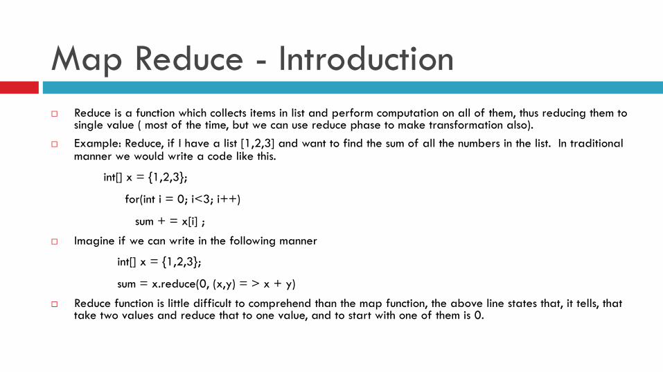
Map Reduce - Introduction ¨ Reduce is a function which collects items in list and perform computation on all of them, thus reducing them to
single value ( most of the time, but we can use reduce phase to make transformation also). ¨ Example: Reduce, if I have a list [1,2,3] and want to find the sum of all the numbers in the list. In traditional
manner we would write a code like this.
int[] x = {1,2,3};
for(int i = 0; i<3; i++)
sum + = x[i] ;
¨ Imagine if we can write in the following manner
int[] x = {1,2,3};
sum = x.reduce(0, (x,y) = > x + y)
¨ Reduce function is little difficult to comprehend than the map function, the above line states that, it tells, that take two values and reduce that to one value, and to start with one of them is 0.
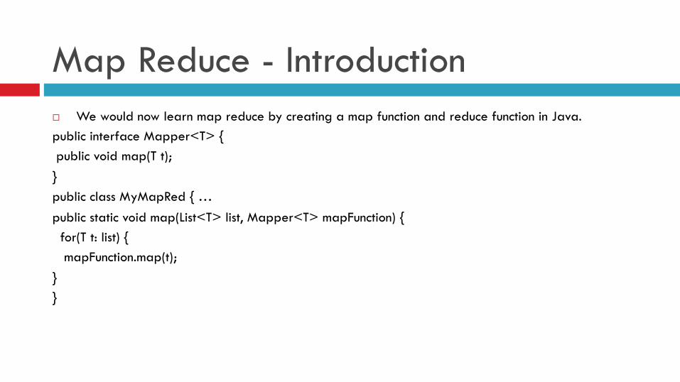
Map Reduce - Introduction ¨ We would now learn map reduce by creating a map function and reduce function in Java. public interface Mapper<T> { public void map(T t); } public class MyMapRed { … public static void map(List<T> list, Mapper<T> mapFunction) { for(T t: list) { mapFunction.map(t); } }
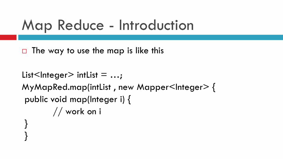
Map Reduce - Introduction ¨ The way to use the map is like this List<Integer> intList = …; MyMapRed.map(intList , new Mapper<Integer> { public void map(Integer i) { // work on i } }
Map Reduce - Introduction
¨ The important things to know in map reduce is the role of key and the values. Programming in map reduce revolves around keys and values.
¨ Map phase extracts keys and gets values, and in the reduce phase, only one reducer gets a key and all its value.

Map Reduce - Illustration

Map Reduce - Introduction ¨ Map: If all we have to do is to iterate elements in a huge list and apply
some function to each element, in such case the variable part is the function and not the iteration.
¨ Map abstracts the iteration and accepts the array on which it needs to iterate and the function it needs to apply on each element.
¨ Reducer: If all we need to do is to iterate all elements in a huge list and apply some combination function, the variable part is the array and the function and not the iteration.
¨ Reduce abstracts the iteration and accepts array on which it needs to iterate and the function that reduces the array elements into one single value.
Map Reduce - Introduction ¨ When all we need to do is to apply some function to all elements in array, does it
really matter in what order you have to do it. ¨ It does not matter. We can suddenly split the list into two and give them to two
thread and ask them to apply the map function on the elements in the list. ¨ Suddenly the job takes ½ the time it took before the list was split. ¨ See we don’t have the burden on lock and synchronization. In Map Reduce an
element (call it a row ) is looked only by one mapper, and a key is processed by only one reducer, one reducer takes all values of a key and process them.
¨ Hadoop / MR abstracts the concepts behind the map and reduce logic and provided a framework so that, all we need to do is, give the logic that happens in map and the logic that happens in reduce, this is done by implementing map and reduce function.
Map Reduce - Introduction ¨ MR abstracts the concepts of looping. ¨ Please take the pain of learning what it means by functional
programming, as without having an understanding on closure, function object, and functional programming it’s very difficult to comprehend map reduce beyond the superficial level.
¨ To get to the depths of Map Reduce, one need to know the reason behind map and reduce and not just the API level details.
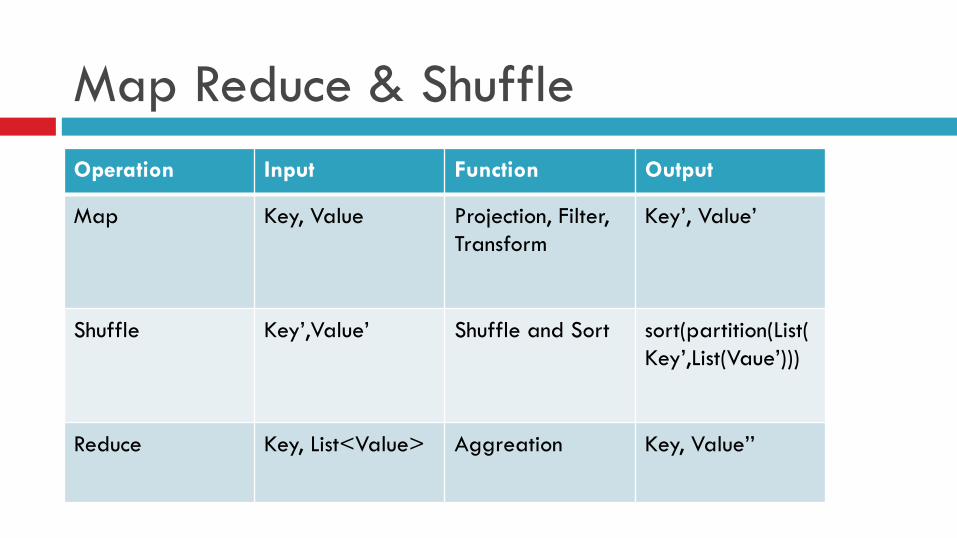
Map Reduce & Shuffle Operation Input Function Output
Map Key, Value Projection, Filter, Transform
Key’, Value’
Shuffle Key’,Value’ Shuffle and Sort sort(partition(List(Key’,List(Vaue’)))
Reduce Key, List<Value> Aggreation Key, Value’’
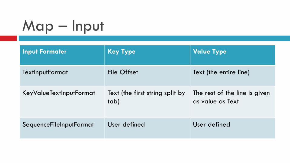
Map – Input Input Formater Key Type Value Type
TextInputFormat File Offset Text (the entire line)
KeyValueTextInputFormat Text (the first string split by tab)
The rest of the line is given as value as Text
SequenceFileInputFormat User defined User defined
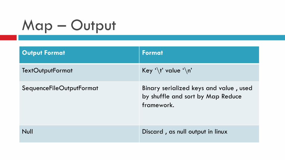
Map – Output Output Format Format
TextOutputFormat Key ‘\t’ value ‘\n’
SequenceFileOutputFormat Binary serialized keys and value , used by shuffle and sort by Map Reduce framework.
Null Discard , as null output in linux
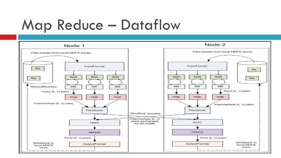
Map Reduce – Dataflow
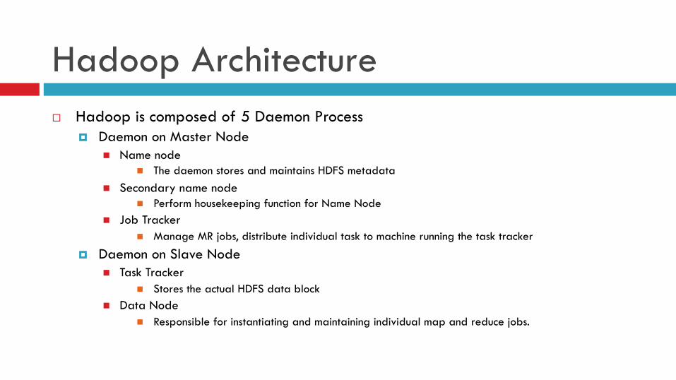
Hadoop Architecture ¨ Hadoop is composed of 5 Daemon Process
¤ Daemon on Master Node n Name node
n The daemon stores and maintains HDFS metadata n Secondary name node
n Perform housekeeping function for Name Node n Job Tracker
n Manage MR jobs, distribute individual task to machine running the task tracker
¤ Daemon on Slave Node n Task Tracker
n Stores the actual HDFS data block n Data Node
n Responsible for instantiating and maintaining individual map and reduce jobs.
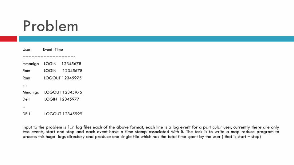
Problem User Event Time
-----------------------------------
mmaniga LOGIN 12345678
Ram LOGIN 12345678
Ram LOGOUT 12345975
…
Mmaniga LOGOUT 12345975
Dell LOGIN 12345977
..
DELL LOGOUT 12345999
Input to the problem is 1..n log files each of the above format, each line is a log event for a particular user, currently there are only two events, start and stop and each event have a time stamp associated with it. The task is to write a map reduce program to process this huge logs directory and produce one single file which has the total time spent by the user ( that is start – stop)
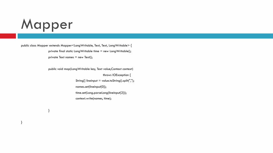
Mapper public class Mapper extends Mapper<LongWritable, Text, Text, LongWritable> {
private final static LongWritable time = new LongWritable();
private Text names = new Text();
public void map(LongWritable key, Text value,Context context)
throws IOException {
String[] lineinput = value.toString().split(",");
names.set(lineinput[0]);
time.set(Long.parseLong(lineinput[2]));
context.write(names, time);
}
}
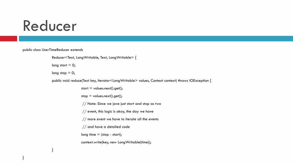
Reducer public class UserTimeReducer extends
Reducer<Text, LongWritable, Text, LongWritable> {
long start = 0;
long stop = 0;
public void reduce(Text key, Iterator<LongWritable> values, Context context) throws IOException {
start = values.next().get();
stop = values.next().get();
// Note: Since we jave just start and stop as two
// event, this logic is okay, the day we have
// more event we have to iterate all the events
// and have a detailed code
long time = (stop - start);
context.write(key, new LongWritable(time));
}
}
Session 5 – Advanced Map Reduce
Map Reduce – Problem Solving ¨ So far we have seen map reduce program where the job was to handle
input from a single file location and multiple files. ¨ Real problems will have multiple input paths, each having different type of
data. ¨ Input formatter for each of those files types might be different, one might
have TextInputFormater and one might have Custom input formatter. ¨ Since each input path holds different type of data, it directly translates
that they might need different mapper function, a single mapper function would no more be sufficient.
¨ We are going to look into problems that have multiple mappers and single reducer.
Map Reduce – Problem Solving ¨ Problem Statement:
¤ A company has a list of user id (user name) and there mobile number. String:UserName, Number:MobileNUmber format.
¤ The company gives the list of mobile number to a third part bulk sms vendor to send sms to all the mobile number, the company does not share the name of the user.
¤ The third party produces a list of mobile number and their sms delivery status and this file is given to the primary company.
¤ The primary company has to create a new file which has name , mobile number and their delivery status. A simple problem to solve in Database as long as data is small.
¤ This is one example of map reduce and how its used to solve real world problems. ¤ This is a join problems map reduce is designed to solve. What we also learn is to
deal with multiple mappers and single reducer concepts.

Map Reduce – Problem Solving ¨ Problem Statement
¤ The problem has two input file types, one is user details and one is delivery details and they have a common data called mobile number.
¤ In database we can do a join to solve this problem.
Name Mobile
Mani 1234
Vijay 2341
Ravi 3452
Mobile Status
1234 0
2431 2
3452 3 Name Mobile Status
Mani 1234 0
Vijay 2341 2
Ravi 3452 3
Map Reduce – Problem Solving ¨ Mapper
¤ We need two mappers, one to process the customer details and one to process the Delivery details.
¤ The key concept is the key, to identify what is the key in each input data and make sure that data from different input files for the same key reaches the same reducer.
¤ In our scenario, the key is the mobile number, so in each of the mapper job find the key from the data and make the remaining things as value and send to mapper.
¨ Mapper problem ¤ How will reducer know which data belong to customer details and which data
belongs to the delivery details. ¤ How do we make sure multiple mappers are run and then the reducer kicks in. ¤ What is there in map reduce framework to solve this problem.
Map Reduce – Graph Problem Solving
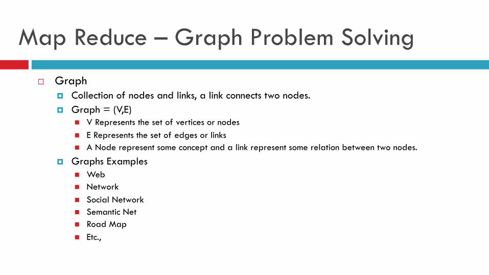
¨ Graph ¤ Collection of nodes and links, a link connects two nodes. ¤ Graph = (V,E)
n V Represents the set of vertices or nodes n E Represents the set of edges or links n A Node represent some concept and a link represent some relation between two nodes.
¤ Graphs Examples n Web n Network n Social Network n Semantic Net n Road Map n Etc.,
Map Reduce – Graph Problem Solving
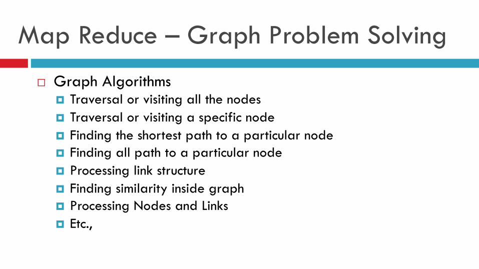
¨ Graph Algorithms ¤ Traversal or visiting all the nodes ¤ Traversal or visiting a specific node ¤ Finding the shortest path to a particular node ¤ Finding all path to a particular node ¤ Processing link structure ¤ Finding similarity inside graph ¤ Processing Nodes and Links ¤ Etc.,
Map Reduce – Graph Problem Solving
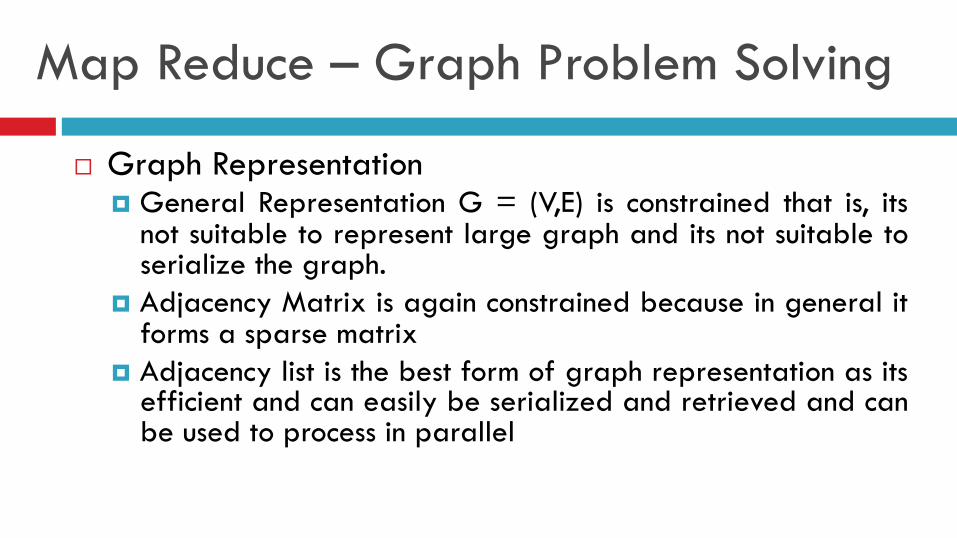
¨ Graph Representation ¤ General Representation G = (V,E) is constrained that is, its
not suitable to represent large graph and its not suitable to serialize the graph.
¤ Adjacency Matrix is again constrained because in general it forms a sparse matrix
¤ Adjacency list is the best form of graph representation as its efficient and can easily be serialized and retrieved and can be used to process in parallel
Map Reduce – Graph Problem Solving
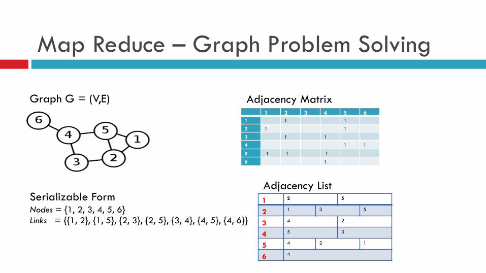
Graph G = (V,E) 1 2 3 4 5 6 1 1 1 2 1 1 3 1 1 4 1 1
5 1 1 1 6 1
Adjacency Matrix
1 2 5
2 1 3 5
3 4 2
4 5 3
5 4 2 1
6 4
Adjacency List Serializable Form Nodes = {1, 2, 3, 4, 5, 6} Links = {{1, 2}, {1, 5}, {2, 3}, {2, 5}, {3, 4}, {4, 5}, {4, 6}}
Map Reduce – Graph Problem Solving
¨ Problem Breadth First Search ¤ Search algorithm on graph, we begin at the root node
(or a starting node) and explore all the adjacent nodes, it then explores their unexplored adjacent nodes, and so on, until it finds the desired node or it completes exploring all the nodes.
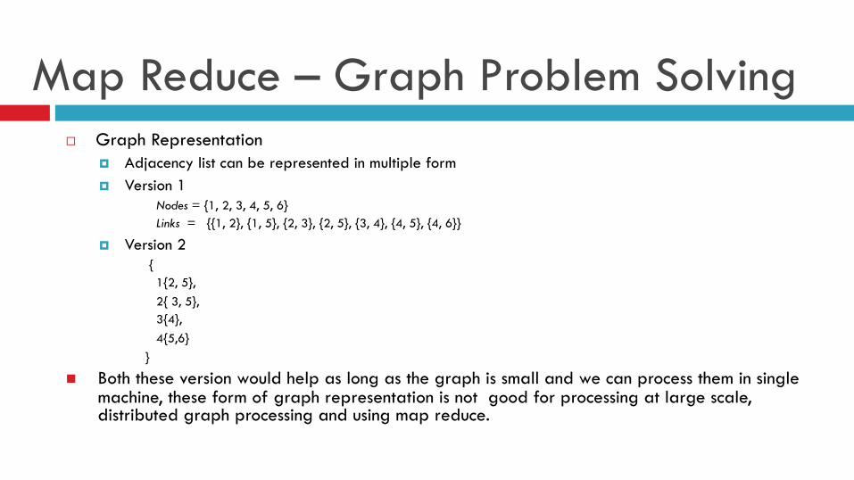
Map Reduce – Graph Problem Solving ¨ Graph Representation
¤ Adjacency list can be represented in multiple form ¤ Version 1
Nodes = {1, 2, 3, 4, 5, 6} Links = {{1, 2}, {1, 5}, {2, 3}, {2, 5}, {3, 4}, {4, 5}, {4, 6}}
¤ Version 2 { 1{2, 5}, 2{ 3, 5}, 3{4}, 4{5,6} }
n Both these version would help as long as the graph is small and we can process them in single machine, these form of graph representation is not good for processing at large scale, distributed graph processing and using map reduce.
Map Reduce – Graph Problem Solving
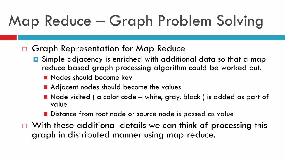
¨ Graph Representation for Map Reduce ¤ Simple adjacency is enriched with additional data so that a map
reduce based graph processing algorithm could be worked out. n Nodes should become key n Adjacent nodes should become the values n Node visited ( a color code – white, gray, black ) is added as part of
value n Distance from root node or source node is passed as value
¨ With these additional details we can think of processing this graph in distributed manner using map reduce.
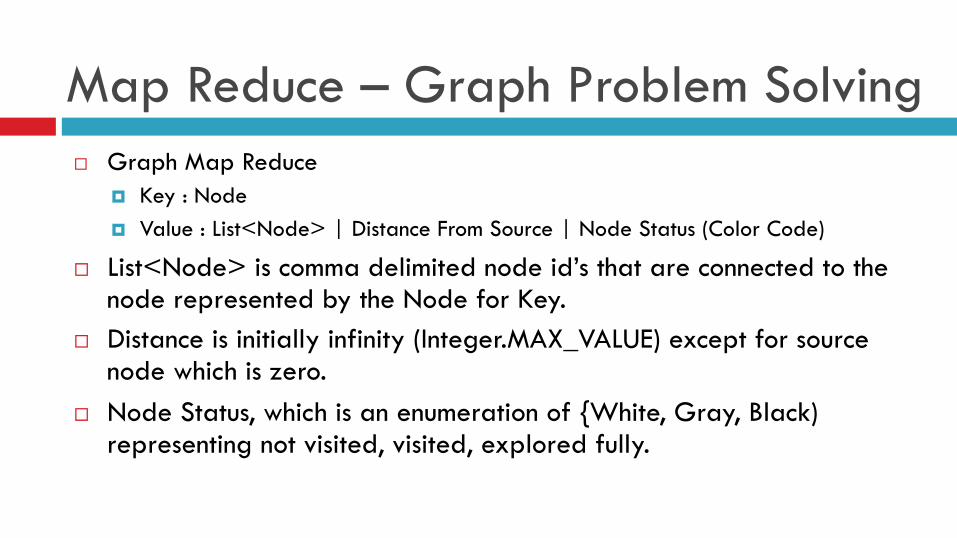
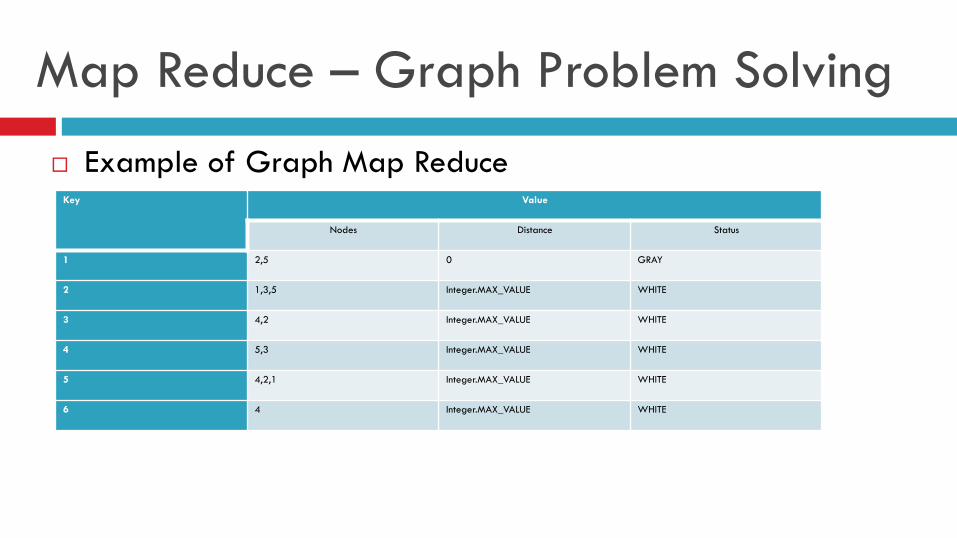
Map Reduce – Graph Problem Solving ¨ Graph Map Reduce
¤ Key : Node ¤ Value : List<Node> | Distance From Source | Node Status (Color Code)
¨ List<Node> is comma delimited node id’s that are connected to the node represented by the Node for Key.
¨ Distance is initially infinity (Integer.MAX_VALUE) except for source node which is zero.
¨ Node Status, which is an enumeration of {White, Gray, Black) representing not visited, visited, explored fully.
Map Reduce – Graph Problem Solving
¨ Example of Graph Map Reduce Key Value
Nodes Distance Status
1 2,5 0 GRAY
2 1,3,5 Integer.MAX_VALUE WHITE
3 4,2 Integer.MAX_VALUE WHITE
4 5,3 Integer.MAX_VALUE WHITE
5 4,2,1 Integer.MAX_VALUE WHITE
6 4 Integer.MAX_VALUE WHITE
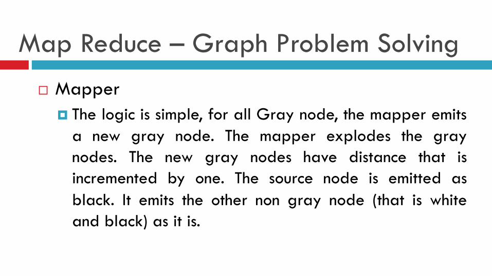
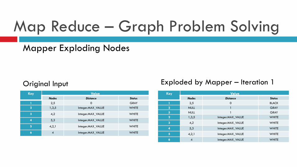
Map Reduce – Graph Problem Solving ¨ Mapper
¤ The logic is simple, for all Gray node, the mapper emits a new gray node. The mapper explodes the gray nodes. The new gray nodes have distance that is incremented by one. The source node is emitted as black. It emits the other non gray node (that is white and black) as it is.
Map Reduce – Graph Problem Solving
Key Value Nodes Distance Status
1 2,5 0 GRAY 2 1,3,5 Integer.MAX_VALUE WHITE
3 4,2 Integer.MAX_VALUE WHITE
4 5,3 Integer.MAX_VALUE WHITE
5 4,2,1 Integer.MAX_VALUE WHITE
6 4 Integer.MAX_VALUE WHITE
Mapper Exploding Nodes
Key Value Nodes Distance Status
1 2,5 0 BLACK 2 NULL 1 GRAY 5 NULL 1 GRAY 2 1,3,5 Integer.MAX_VALUE WHITE
3 4,2 Integer.MAX_VALUE WHITE
4 5,3 Integer.MAX_VALUE WHITE
5 4,2,1 Integer.MAX_VALUE WHITE
6 4 Integer.MAX_VALUE WHITE
Original Input Exploded by Mapper – Iteration 1
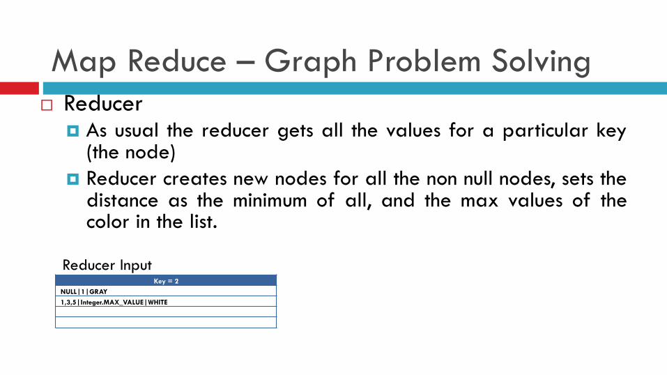
Map Reduce – Graph Problem Solving ¨ Reducer
¤ As usual the reducer gets all the values for a particular key (the node)
¤ Reducer creates new nodes for all the non null nodes, sets the distance as the minimum of all, and the max values of the color in the list.
Key = 2 NULL|1|GRAY 1,3,5|Integer.MAX_VALUE|WHITE
Reducer Input
Map Reduce – Graph Problem Solving
Key Value Nodes Distance Status
1 2,5 0 BLACK 2 1,3,5 1 GRAY 3 4,2 Integer.MAX_VALUE WHITE 4 5,3 Integer.MAX_VALUE WHITE 5 4,2,1 Integer.MAX_VALUE WHITE 6 4 Integer.MAX_VALUE WHITE
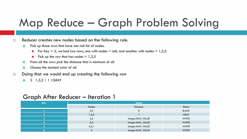
¨ Reducer creates new nodes based on the following rule. ¤ Pick up those rows that have non null list of nodes.
n For Key = 2, we had two rows, one with nodes = null, and another with nodes = 1,3,5 n Pick up the row that has nodes = 1,3,5
¤ From all the rows pick the distance that is minimum of all ¤ Choose the darkest color of all.
¨ Doing that we would end up creating the following row ¤ 2 1,3,5 | 1 |GRAY
Graph After Reducer – Iteration 1
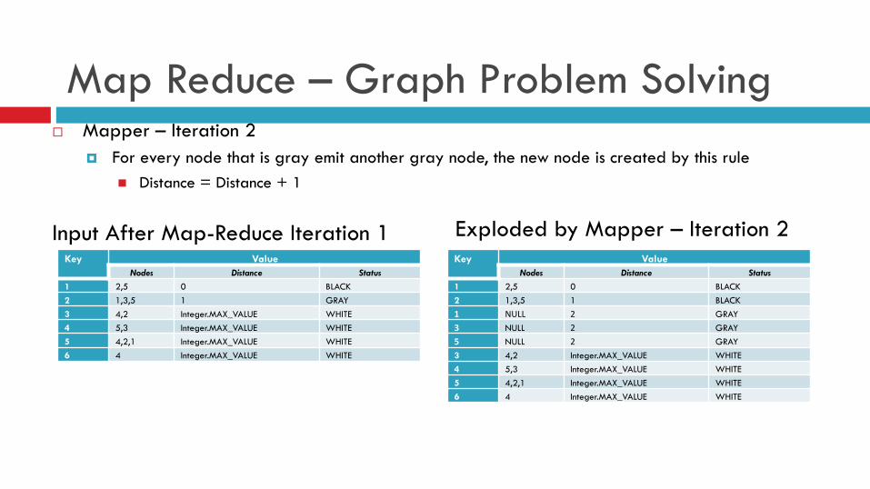
Map Reduce – Graph Problem Solving ¨ Mapper – Iteration 2
¤ For every node that is gray emit another gray node, the new node is created by this rule n Distance = Distance + 1
Input After Map-Reduce Iteration 1 Exploded by Mapper – Iteration 2 Key Value
Nodes Distance Status 1 2,5 0 BLACK 2 1,3,5 1 GRAY 3 4,2 Integer.MAX_VALUE WHITE 4 5,3 Integer.MAX_VALUE WHITE 5 4,2,1 Integer.MAX_VALUE WHITE 6 4 Integer.MAX_VALUE WHITE
Key Value Nodes Distance Status
1 2,5 0 BLACK 2 1,3,5 1 BLACK 1 NULL 2 GRAY 3 NULL 2 GRAY 5 NULL 2 GRAY 3 4,2 Integer.MAX_VALUE WHITE 4 5,3 Integer.MAX_VALUE WHITE 5 4,2,1 Integer.MAX_VALUE WHITE 6 4 Integer.MAX_VALUE WHITE
Map Reduce – Graph Problem Solving
Key Value Nodes Distance Status
1 2,5 0 BLACK 1 NULL 2 GRAY
Key Value Nodes Distance Status
2 1,3,5 1 BLACK
Key Value Nodes Distance Status
3 NULL 2 GRAY 3 4,2 Integer.MAX_VALUE WHITE
Key Value Nodes Distance Status
5 NULL 2 GRAY 5 4,2,1 Integer.MAX_VALUE WHITE
Key Value Nodes Distance Status
6 4 Integer.MAX_VALUE WHITE
Key Value Nodes Distance Status
4 5,3 Integer.MAX_VALUE WHITE
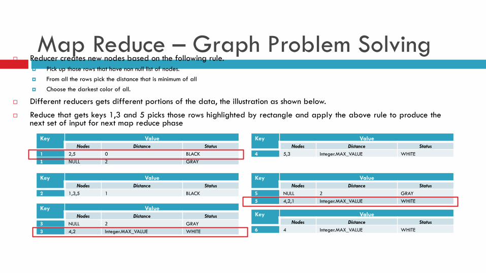
¨ Reducer creates new nodes based on the following rule. ¤ Pick up those rows that have non null list of nodes.
¤ From all the rows pick the distance that is minimum of all
¤ Choose the darkest color of all.
¨ Different reducers gets different portions of the data, the illustration as shown below.
¨ Reduce that gets keys 1,3 and 5 picks those rows highlighted by rectangle and apply the above rule to produce the next set of input for next map reduce phase
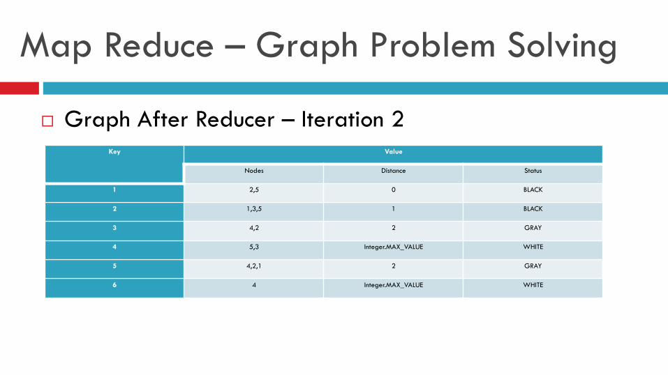
Map Reduce – Graph Problem Solving
¨ Graph After Reducer – Iteration 2 Key Value
Nodes Distance Status
1 2,5 0 BLACK
2 1,3,5 1 BLACK
3 4,2 2 GRAY
4 5,3 Integer.MAX_VALUE WHITE
5 4,2,1 2 GRAY
6 4 Integer.MAX_VALUE WHITE
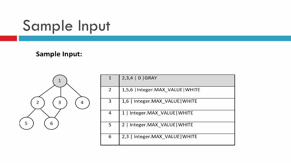
Sample Input
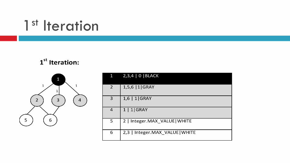
1st Iteration
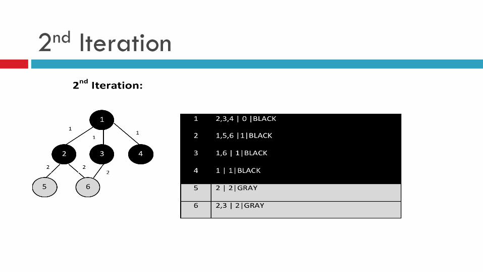
2nd Iteration
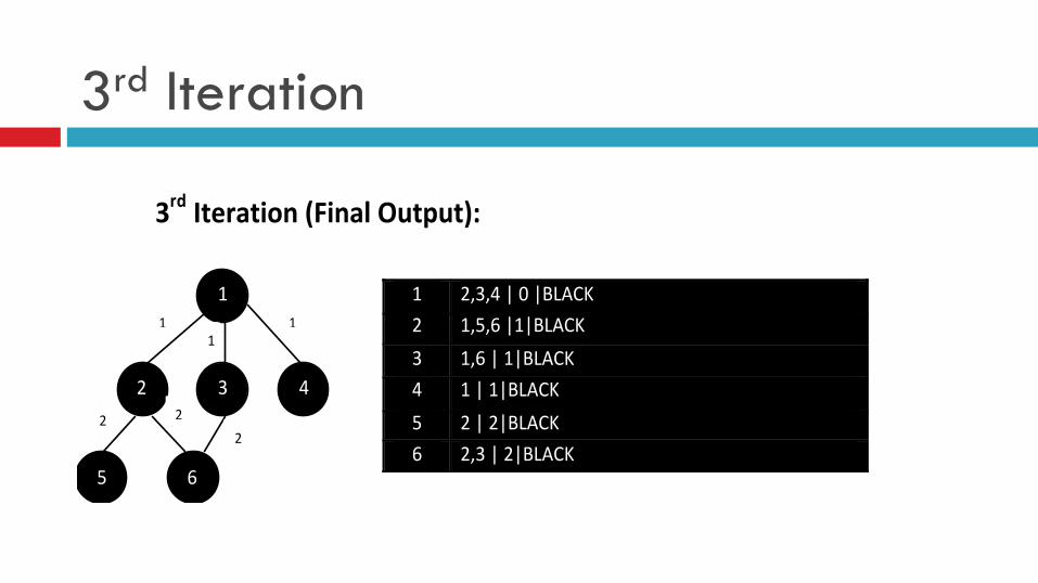
3rd Iteration
3rd$Iteration$(Final$Output):$
!
!1! 2,3,4!|!0!|BLACK!2! 1,5,6!|1|BLACK!3! 1,6!|!1|BLACK!4! 1!|!1|BLACK!5! 2!|!2|BLACK!6! 2,3!|!2|BLACK!
1!
2! 3!
5!
4!
6!
1!1!
1!
2! 2!2!
Welcome NoSQL
¨ Why NoSQL ? ¨ Why ACID is not relevant anymore? ¨ Do recent web apps have different needs than
yesterday applications? ¨ What changed recently?
NoSQL ¨ What Changed
¤ Massive data volumes ¤ Extreme query load
n Bottleneck is joins ¤ Schema evolution
n Its almost impossible to have a fixed schema for web sale database.
n With NoSQL schema changes can be gradually introduced into the system.
No SQL Limitation ¨ Limited query capabilities ¨ Eventual consistency is not
intuitive to programing, it makes client applications more complicated
¨ No standardization ¨ Portability might be an issue ¨ Insufficient access control
Advantage ¨ High availability ¨ Lower cost ¨ predictable elasticity ¨ Schema flexibility ¨ Sparse and semi-structured
data
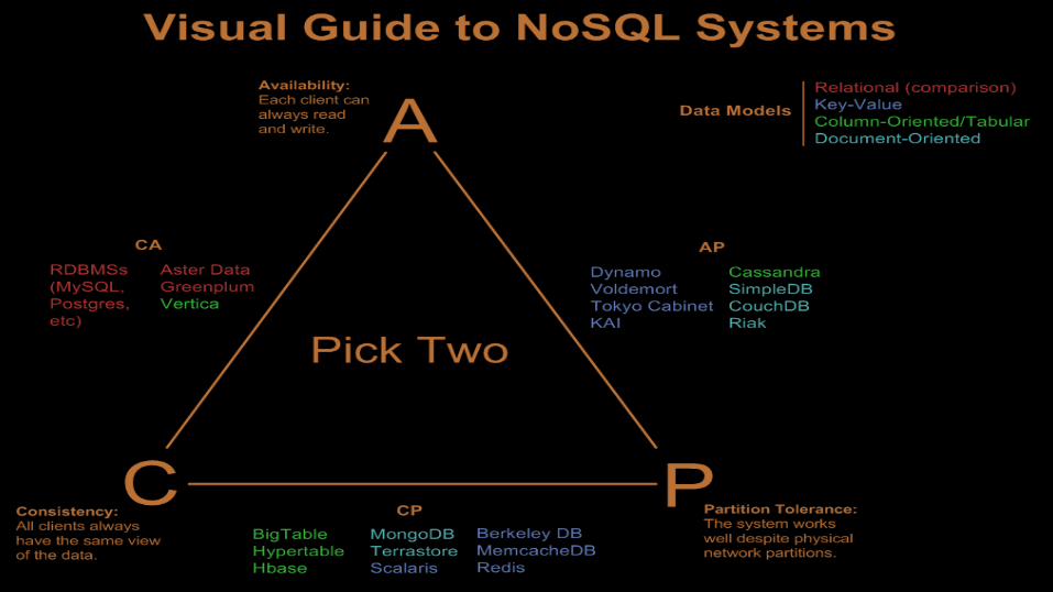
CAP Theorem ¨ In theoretical computer science the CAP theorem, also known as Brewer's
theorem, states that it is impossible for a distributed computer system to simultaneously provide all three of the following guarantees: ¤ Consistency (all nodes see the same data at the same time) ¤ Availability (a guarantee that every request receives a response about whether
it was successful or failed) ¤ Partition tolerance (the system continues to operate despite arbitrary message
loss) ¨ According to the theorem, a distributed system can satisfy any two of these
guarantees at the same time, but not all three
CAP Theorem ¨ “Consistency” means that if someone writes a value to a database,
thereafter other users will immediately be able to read the same value back
¨ “Availability” means that if some number of nodes fail in your cluster the distributed system can remain operational, and
¨ “Tolerance to Partitions” means that if the nodes in your cluster are divided into two groups that can no longer communicate by a network failure, again the system remains operational.
CAP Theorem ¨ Consistent and Available
¤ Single site clusters, when a partition occurs the system blocks ¤ Have trouble with partitions and typically deal with it with replication
¨ Consistent and Tolerant to Partition ¤ Some data might become inaccessable (thus sacrificing availablity), but the rest of the
system is consistent(that is accurate) ¤ Have trouble with availability while keeping data consistent across partitioned nodes
¨ Available and Tolerant to Partition ¤ System is available under partition, but it might return stale / inaccurate data ¤ Achieve "eventual consistency" through replication and verification ¤ Example DNS server
Database ¨ No SQL database falls broadly into the following category
¤ Key Value Store n A Distributed hash table n Support get, put, and delete operations based on a primary key.
¤ Column Store n Each key is associated with many attributes (a map of map) n Still use tables but have no joins (joins must be handled in application). n Store data by column as opposed to traditional row-oriented databases. Aggregations is much easier.
¤ Document Store n Stores semi structured data, example JSON n It's very easy to map data from object-oriented software to these systems n Map/Reduce based materialization for aggregated queries
¤ Graph Database
Database ¨ Key Value
¤ Dynamo ¤ Voldemort
¨ Column ¤ HBase ¤ Cassandra ¤ BigTable
¨ Document Database ¤ MongoDB ¤ CouchDB
Session 6 - HBase ¨ Advanced Introduction to HBase ¨ CAP Theorem and Eventual consistency ¨ Learning NoSQL ¨ Creating Table – Shell and Programming ¨ Understanding Column Families ¨ Unlearning Entity Relation ¨ Learning Column Value & Key Pair ¨ Unlearning Index & Query ¨ Learning Scan ¨ MapReduce and HBase – Importing into HBase
HBase – Advanced Introduction ¨ Open Source, horizontally scalable, sorted map data built
on top of Apache Hadoop. ¨ Datamodel inspired and similar to Google’s BigTable. ¨ Goal is to provide quick random read / write access to
massive amount od structured data. ¨ Layered over HDFS ¨ Tolerant of Machine Failures ¨ Strong Consistency model
HBase Features ¨ Strongly consistent reads/writes. ¨ Automatic sharding: HBase tables are distributed on the cluster via regions, and regions are
automatically split and re-distributed as your data grows. ¨ Automatic RegionServer failover ¨ Hadoop/HDFS Integration: HBase supports HDFS out of the box as it's distributed file system. ¨ MapReduce: HBase supports massively parallelized processing via MapReduce for using
HBase as both source and sink. ¨ Java Client API: HBase supports an easy to use Java API for programmatic access. ¨ Thrift/REST API: HBase also supports Thrift and REST for non-Java front-ends. ¨ Operational Management: HBase provides build-in web-pages for operational insight as well
as JMX metrics.
When HBase ¨ If we have hundreds of millions or billions of rows, then HBase is a good candidate. ¨ If we have a few thousand/million rows, then using a traditional RDBMS might be a better
choice. ¨ If we can we live without the extra features that an RDBMS provides (e.g., typed columns,
secondary indexes, transactions, advanced query languages, etc.) ¨ An application built against an RDBMS cannot be "ported" to HBase by simply changing a
JDBC driver. ¨ Consider moving from an RDBMS to HBase as a complete redesign as opposed to a port. ¨ There should be enough hardware. Even HDFS doesn't do well with anything less than 5
DataNodes (due to things such as HDFS block replication which has a default of 3), plus a NameNode.
¨ HBase can run quite well stand-alone on a laptop - but this should be considered a development configuration only.
HDFS vs HBase ¨ HDFS is a distributed file system that is well suited for
the storage of large files. It's documentation states that it is not, however, a general purpose file system, and does not provide fast individual record lookups in files.
¨ HBase, on the other hand, is built on top of HDFS and provides fast record lookups (and updates) for large tables.
¨ HBase internally puts data in indexed "StoreFiles" that exist on HDFS for high-speed lookups
HBase Architecture
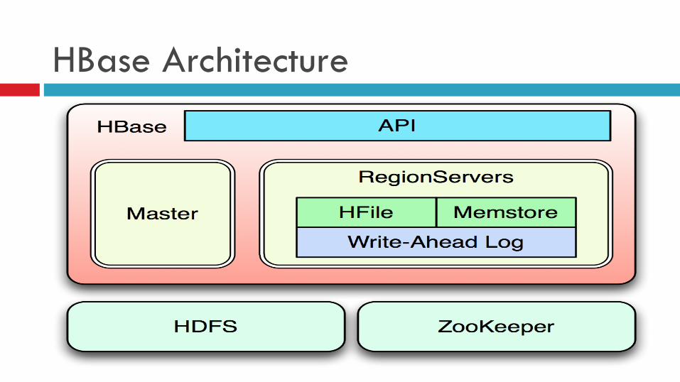
HBase Architecture ¨ Uses HDFS as its reliable storage layer ¨ Access through native Java API, Avro, Thrift, REST,
etc., ¨ Master manages cluster ¨ RegionServer manages data ¨ ZooKeeper for bootstrapping and coordinating the
cluster
HBase Architecture ¨ What is missing (in HDFS), though, is the ability to access data randomly and in close to real-
time ¨ It’s good with a few very, very large files, but not as good with millions of tiny files. ¨ The more files, the higher the pressure on the memory of the NameNode. ¨ Hbase was designed to drive interactive applications, such as Mail or Analytics, while making
use of the same infrastructure and relying on HDFS for replication and data availability. ¨ The data stored is composed of much smaller entities ¨ Transparently take care of aggregating small records into very large storage files ¨ Indexing allows the user to retrieve data with a minimal number of disk seeks. ¨ Hbase could in theory can store the entire web crawl and work with MapReduce to build the
entire search index in a timely manner.
Tables, Rows, Columns, and Cells ¨ the most basic unit is a column. ¨ One or more columns form a row that is addressed uniquely by a row key. ¨ A number of rows, in turn, form a table, and there can be many of them. ¨ Each column may have multiple versions, with each distinct value contained
in a separate cell. ¨ Rows are composed of columns, and those, in turn, are grouped into column
families. ¨ Columns are often referenced as family:qualifier with the qualifier being
any arbitraryarray of bytes.
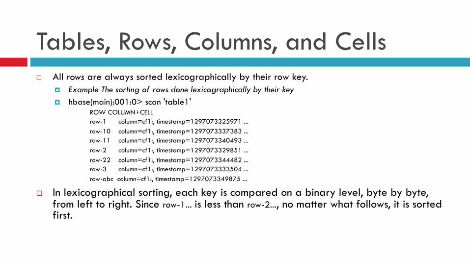
Tables, Rows, Columns, and Cells ¨ All rows are always sorted lexicographically by their row key.
¤ Example The sorting of rows done lexicographically by their key ¤ hbase(main):001:0> scan 'table1'
ROW COLUMN+CELL row-1 column=cf1:, timestamp=1297073325971 ... row-10 column=cf1:, timestamp=1297073337383 ... row-11 column=cf1:, timestamp=1297073340493 ... row-2 column=cf1:, timestamp=1297073329851 ... row-22 column=cf1:, timestamp=1297073344482 ... row-3 column=cf1:, timestamp=1297073333504 ... row-abc column=cf1:, timestamp=1297073349875 ...
¨ In lexicographical sorting, each key is compared on a binary level, byte by byte, from left to right. Since row-1... is less than row-2..., no matter what follows, it is sorted first.
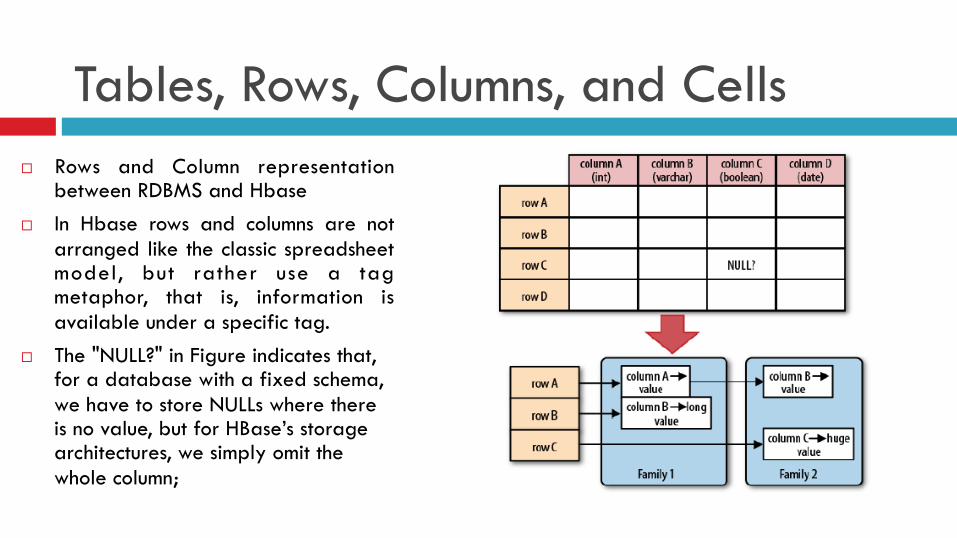
Tables, Rows, Columns, and Cells ¨ Rows and Column representation
between RDBMS and Hbase ¨ In Hbase rows and columns are not
arranged like the classic spreadsheet model, but rather use a tag metaphor, that is, information is available under a specific tag.
¨ The "NULL?" in Figure indicates that, for a database with a fixed schema, we have to store NULLs where there is no value, but for HBase’s storage architectures, we simply omit the whole column;
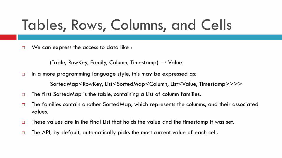
Tables, Rows, Columns, and Cells ¨ We can express the access to data like :
(Table, RowKey, Family, Column, Timestamp) → Value
¨ In a more programming language style, this may be expressed as:
SortedMap<RowKey, List<SortedMap<Column, List<Value, Timestamp>>>>
¨ The first SortedMap is the table, containing a List of column families.
¨ The families contain another SortedMap, which represents the columns, and their associated values.
¨ These values are in the final List that holds the value and the timestamp it was set.
¨ The API, by default, automatically picks the most current value of each cell.
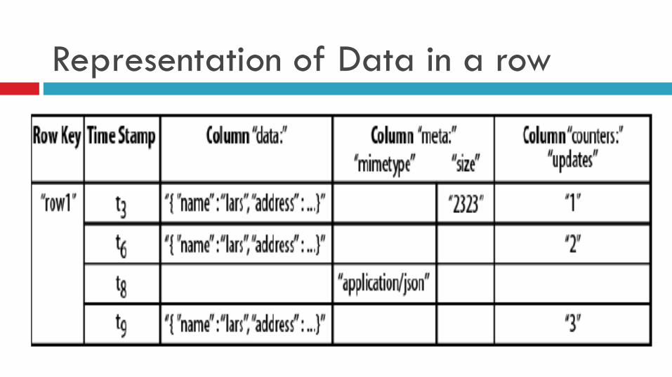
Representation of Data in a row
HBase Simple use case - WebIndex ¨ To store web pages as we crawl internet ¨ Row key is the reversed URL of the page—for example, org.hbase.www. ¨ Column family
¤ To storing the actual HTML code ¤ To store the contents family ¤ Anchor, which is used to store outgoing links ¤ Anchor, to store inbound links ¤ To store metadata like language.
¨ Using multiple versions for the contents family we can save a few older copies of the HTML, and is helpful when we have to analyze how often a page changes,
Access and Atomicity ¨ Access to row data is atomic and includes any number
of columns being read or written to. ¨ No further guarantee or transactional feature that
spans multiple rows or across tables. ¨ This atomic access is a contributing factor to this
architecture being strictly consistent, as each concurrent reader and writer can make safe assumptions about the state of a row.
Sharading, Scalability, Load Balancing
¨ The basic unit of scalability and load balancing in HBase is called a region.
¨ Regions are essentially contiguous ranges of rows stored together.
¨ They are dynamically split by the system when they become too large.
¨ Alternatively, they may also be merged to reduce their number and required storage files.
Region, Region Server, Split ¨ Initially there is only one region for a table ¨ As data grows, the system ensure that it does not exceed the
configured maximum size. ¨ On reaching max, the region is split into two at the middle
key—the row key in the middle of the region—creating two roughly equal halves
¨ Each region is served by exactly one region server, and each of these servers can serve many regions at any time
FileSystem Metadata ¨ Meta-data in Memory
– The entire metadata is in main memory – No demand paging of meta-data
¨ Types of Metadata – List of files – List of Blocks for each file – List of DataNodes for each block – File attributes, e.g creation time, replication factor
¨ A Transaction Log – Records file creations, file deletions. etc
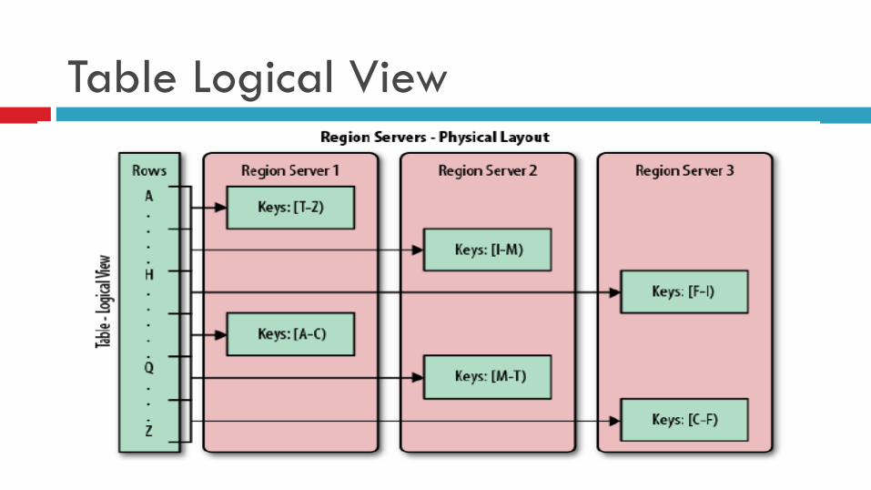
Table Logical View
Session – 7 HDFS Introduction
HDFS File System Namespace ¨ Hierarchical file system with directories and files ¨ Can Create, remove, move, rename etc. ¨ Namenode maintains the file system namespace ¨ Any meta information changes to the file system namespace
or its properties is recorded by the Namenode. ¨ An application can specify the number of replicas of the file
needed: replication factor of the file. This information is stored in the Namenode.
HDFS Data Replication � HDFS is designed to store very large files across machines in a large cluster. � Stores each file as a sequence of blocks. � All blocks in the file except the last are of the same size. � Blocks are replicated for fault tolerance. � Block size and replicas are configurable per file, applications can specify the
number of replicas of a file � Replication factor can be specified at file creation time and can be changed later � The Namenode receives a Heartbeat and a BlockReport from each DataNode in the
cluster. � Receipt of a Heartbeat implies that the DataNode is functioning properly. A
Blockreport contains a list of all blocks on a DataNode.
HDFS Replica � The placement of the replicas is critical to HDFS reliability and performance.
� Optimizing replica placement distinguishes HDFS from other distributed file systems.
� Rack-aware replica placement: ¡ Goal: improve reliability, availability and network bandwidth utilization
� Many racks, communication between racks are through switches.
� Network bandwidth between machines on the same rack is greater than those in different racks.
� Namenode determines the rack id for each DataNode.
� Replicas are typically placed on unique racks ¡ Simple but non-optimal, prevents loosing data when an entire rack fails and allows use bandwidth of multiple rack when reading data
¡ Evenly distribute replicas in cluster making load balance easy but also makes writes expensive as data need to be sent to multiple rack
¡ Replication factor is 3
� Replicas are placed: one on a node in a local rack, one on a different node in the local rack and one on a node in a different rack.
� 1/3 of the replica on a node, 2/3 on a rack and 1/3 distributed evenly across remaining racks.
Replica Selection
¨ Replica selection for Read operation: HDFS tries to minimize the bandwidth consumption and latency by selecting a replica that is closer to the reader.
¨ If there is a replica on the Reader node then that is preferred.
¨ HDFS cluster may span multiple data centers: replica in the local data center is preferred over the remote one.
NameNode safemode � On startup Namenode enters Safemode. � Replication of data blocks do not occur in Safemode. � Each DataNode checks in with Heartbeat and BlockReport. � Namenode verifies that each block has acceptable number of replicas � After a configurable percentage of safely replicated blocks check in with
the Namenode, Namenode exits Safemode. � It then makes the list of blocks that need to be replicated. � Namenode then proceeds to replicate these blocks to other Datanodes.
FileSystem Metadata ¨ The HDFS namespace is stored by Namenode. ¨ Namenode uses a transaction log called the EditLog to record every
change that occurs to the filesystem meta data. ¤ For example, creating a new file. ¤ Change replication factor of a file ¤ EditLog is stored in the Namenode’s local filesystem
¨ Entire filesystem namespace including mapping of blocks to files and file system properties is stored in a file FsImage. Stored in Namenode’s local filesystem.
FileSystem Namenode � Keeps image of entire file system namespace and file Blockmap in
memory. � 4GB of local RAM is sufficient to support the above data structures
that represent the huge number of files and directories. � When the Namenode starts up it gets the FsImage and Editlog from
its local file system, update FsImage with EditLog information and then stores a copy of the FsImage on the filesytstem as a checkpoint.
� Periodic checkpointing is done. So that the system can recover back to the last checkpointed state in case of a crash.
FileSystem DataNode � A Datanode stores data in files in its local file system. � Datanode has no knowledge about HDFS filesystem � It stores each block of HDFS data in a separate file. � Datanode does not create all files in the same directory. � It uses heuristics to determine optimal number of files per
directory and creates directories appropriately: � When the filesystem starts up it generates a list of all HDFS
blocks and send this report to Namenode: Blockreport.
FileSystem DataNode ¨ A Block Server
– Stores data in the local file system (e.g. ext3) – Stores meta-data of a block (e.g. CRC) – Serves data and meta-data to Clients
¨ Block Report – Periodically sends a report of all existing blocks to the NameNode
¨ Facilitates Pipelining of Data – Forwards data to other specified DataNodes

HDFS Communication Protocol � All HDFS communication protocols are layered on top of the TCP/IP
protocol � A client establishes a connection to a configurable TCP port on the
Namenode machine. It talks ClientProtocol with the Namenode. � The Datanodes talk to the Namenode using Datanode protocol. � RPC abstraction wraps both ClientProtocol and Datanode protocol. � Namenode is simply a server and never initiates a request; it only
responds to RPC requests issued by DataNodes or clients.
HDFS Robustness
¨ Primary objective of HDFS is to store data reliably in the presence of failures.
¨ Three common failures are: Namenode failure, Datanode failure and network partition
DataNode failure and heartbeat ¨ A network partition can cause a subset of Datanodes to lose connectivity with the Namenode. ¨ Namenode detects this condition by the absence of a Heartbeat message. ¨ Namenode marks Datanodes without Hearbeat and does not send any IO requests to them. ¨ Any data registered to the failed Datanode is not available to the HDFS. ¨ Also the death of a Datanode may cause replication factor of some of the blocks to fall below
their specified value. ¨ NameNode constantly tracks which blocks need to be replicated and initiates replication
whenever necessary. The necessity for re-replication may arise due to many reasons: a DataNode may become unavailable, a replica may become corrupted, a hard disk on a DataNode may fail, or the replication factor of a file may be increased.
Data Integrity ¨ Consider a situation: a block of data fetched from Datanode arrives
corrupted. ¨ This corruption may occur because of faults in a storage device,
network faults, or buggy software. ¨ A HDFS client creates the checksum of every block of its file and
stores it in hidden files in the HDFS namespace. ¨ When a clients retrieves the contents of file, it verifies that the
corresponding checksums match. ¨ If does not match, the client can retrieve the block from a replica.
Disk Failure ¨ FsImage and the EditLog are central data structures of HDFS. A corruption of these
files can cause the HDFS instance to be non-functional. ¨ NameNode can be configured to support maintaining multiple copies of the
FsImage and EditLog. ¨ Any update to either the FsImage or EditLog causes each of the FsImages and
EditLogs to get updated synchronously. ¨ When a NameNode restarts, it selects the latest consistent FsImage and EditLog to
use. ¨ The NameNode machine is a single point of failure for an HDFS cluster. If the
NameNode machine fails, manual intervention is necessary. Currently, automatic restart and failover of the NameNode software to another machine is not supported.
Staging ¨ A client request to create a file does not reach Namenode immediately. ¨ HDFS client caches the data into a temporary file. When the data reached a HDFS block size
the client contacts the Namenode. ¨ Namenode inserts the filename into its hierarchy and allocates a data block for it. ¨ The Namenode responds to the client with the identity of the Datanode and the destination of
the replicas (Datanodes) for the block. ¨ Then the client flushes it from its local memory. ¨ The client sends a message that the file is closed. ¨ Namenode proceeds to commit the file for creation operation into the persistent store. ¨ If the Namenode dies before file is closed, the file is lost. ¨ This client side caching is required to avoid network congestion;
Data Pipelining ¨ Client retrieves a list of DataNodes on which to place replicas of a block
¨ Client writes block to the first DataNode
¨ The first DataNode forwards the data to the next DataNode in the Pipeline
¨ When all replicas are written, the Client moves on to write the next block in file
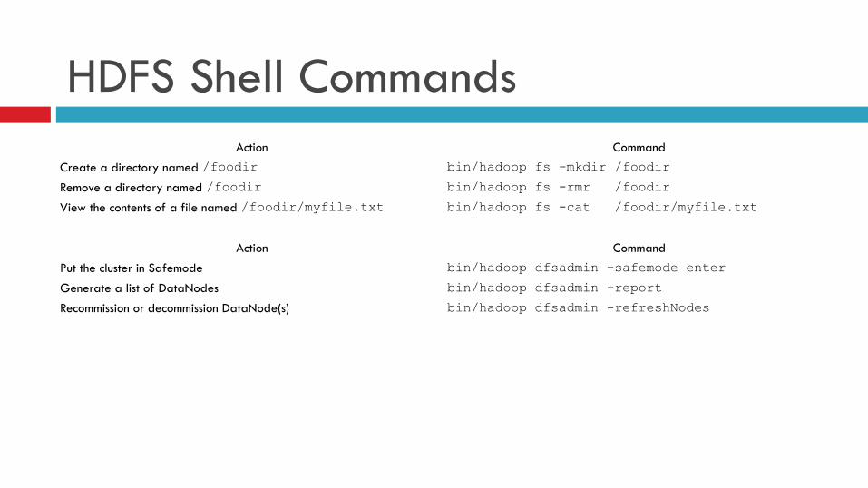
HDFS Shell Commands Action Command
Create a directory named /foodir bin/hadoop fs -mkdir /foodir
Remove a directory named /foodir bin/hadoop fs -rmr /foodir
View the contents of a file named /foodir/myfile.txt bin/hadoop fs -cat /foodir/myfile.txt
Action Command
Put the cluster in Safemode bin/hadoop dfsadmin -safemode enter
Generate a list of DataNodes bin/hadoop dfsadmin -report
Recommission or decommission DataNode(s) bin/hadoop dfsadmin -refreshNodes
Session – 8 Hbase Architecture

HBase Architecture
Master ¨ Master server is responsible for handling load balancing of regions
across region servers, ¨ To unload busy servers and move regions to less occupied ones. ¨ Master is not part of the actual data storage or retrieval path. ¨ It negotiates load balancing and maintains the state of the cluster,
but never provides any data services to either the region servers or the clients.
¨ It takes care of schema changes and other metadata operations, such as creation of tables and column families.
Region Server ¨ Region servers are responsible for all read and
write requests for all regions they serve ¨ They split regions that have exceeded the
configured region size thresholds. ¨ Clients communicate directly with them to handle all
data-related operations.
Auto Shrading ¨ Unit of scalability in Hbase is the Region ¨ Sorted, contiguous range of rows ¨ Spread “randomly ”across RegionServer ¨ Moved around for load balancing and failover ¨ Split automatically or manually to scale with growing
data ¨ Capacity is solely a factor of cluster nodes vs.
regionspernode

HBase ACID ¨ HBase not ACID-compliant, but does guarantee certain specific
properties ¤ Atomicity
n All mutations are atomic within a row. Any put will either wholely succeed or wholely fail.
n APIs that mutate several rows will not be atomic across the multiple rows. n The order of mutations is seen to happen in a well-defined order for each
row, with no interleaving. ¤ Consistency and Isolation
n All rows returned via any access API will consist of a complete row that existed at some point in the table's history.
HBase ACID ¤ Consistency of Scans
n A scan is not a consistent view of a table. Scans do not exhibit snapshot isolation. n Those familiar with relational databases will recognize this isolation level as "read
committed". ¤ Durability
n All visible data is also durable data. That is to say, a read will never return data that has not been made durable on disk.
n Any operation that returns a "success" code (e.g. does not throw an exception) will be made durable.
n Any operation that returns a "failure" code will not be made durable (subject to the Atomicity guarantees above).
n All reasonable failure scenarios will not affect any of the listed ACID guarantees.
Hfile and HDFS Block ¨ The default block size for files in HDFS is 64 MB, which is 1,024
times the HFile default block size (64kb). ¨ HBase storage file blocks do not match the Hadoop blocks. There is
no correlation between these two block types. ¨ HBase stores its files transparently into a filesystem. ¨ HDFS also does not know what HBase stores; it only sees binary files. ¨ HFile content spread across HDFS blocks when many smaller HFile
blocks are transparently stored in two HDFS blocks that are much larger
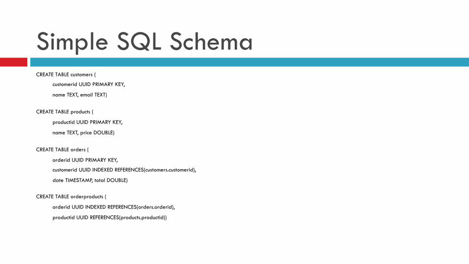
Simple SQL Schema CREATE TABLE customers (
customerid UUID PRIMARY KEY,
name TEXT, email TEXT)
CREATE TABLE products (
productid UUID PRIMARY KEY,
name TEXT, price DOUBLE)
CREATE TABLE orders (
orderid UUID PRIMARY KEY,
customerid UUID INDEXED REFERENCES(customers.customerid),
date TIMESTAMP, total DOUBLE)
CREATE TABLE orderproducts (
orderid UUID INDEXED REFERENCES(orders.orderid),
productid UUID REFERENCES(products.productid))
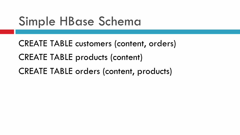
Simple HBase Schema CREATE TABLE customers (content, orders) CREATE TABLE products (content) CREATE TABLE orders (content, products)
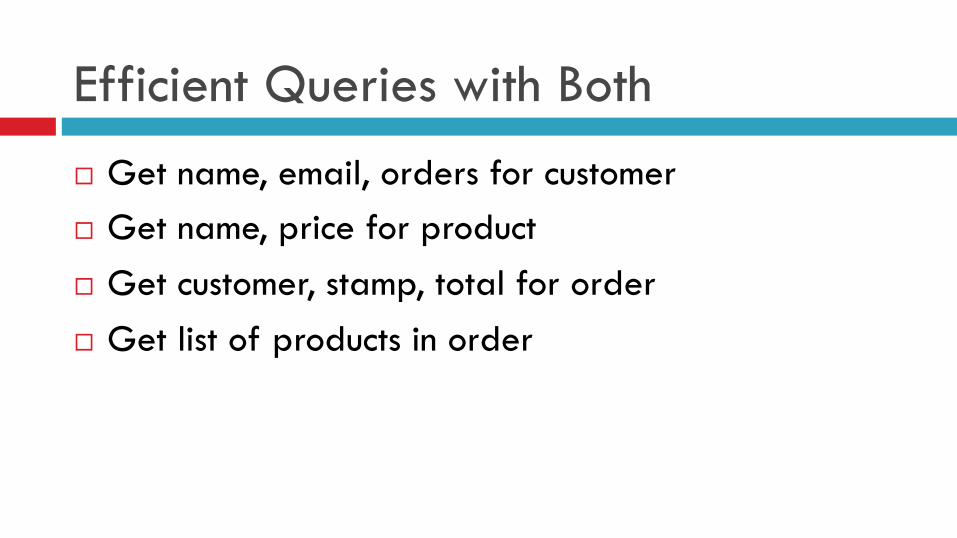
Efficient Queries with Both ¨ Get name, email, orders for customer ¨ Get name, price for product ¨ Get customer, stamp, total for order ¨ Get list of products in order
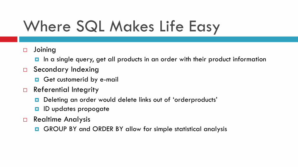
Where SQL Makes Life Easy ¨ Joining
¤ In a single query, get all products in an order with their product information ¨ Secondary Indexing
¤ Get customerid by e-mail ¨ Referential Integrity
¤ Deleting an order would delete links out of ‘orderproducts’ ¤ ID updates propogate
¨ Realtime Analysis ¤ GROUP BY and ORDER BY allow for simple statistical analysis
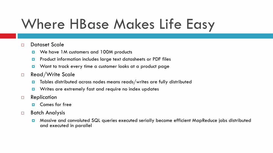
Where HBase Makes Life Easy ¨ Dataset Scale
¤ We have 1M customers and 100M products ¤ Product information includes large text datasheets or PDF files ¤ Want to track every time a customer looks at a product page
¨ Read/Write Scale ¤ Tables distributed across nodes means reads/writes are fully distributed ¤ Writes are extremely fast and require no index updates
¨ Replication ¤ Comes for free
¨ Batch Analysis ¤ Massive and convoluted SQL queries executed serially become efficient MapReduce jobs distributed
and executed in parallel
Hive - Introduction ¨ If we need a large warehouse – Multi petabyte of
data. ¨ Want to leverage SQL knowledge. ¨ Want to leverage hadoop stack and technology to
do warehousing and analytics.
Hive - Introduction ¨ Hadoop based system for querying and analyzing
large volumes of STRUCTURED Data. ¨ Hive uses map reduce for execution ¨ Hive uses HDFS for storage ¨ Hive uses RDBMS for metadata / schema storage,
Derby is the default RDBMS but can be changed to MySQL.
Hive – Where not to use ¨ If data does not cross GB’s. ¨ If we don’t need schema or brining in schema is
difficult or not possible on the data at hand. ¨ If we need response in seconds, and for low latency
application. ¨ If RDBMS can solve, don’t invest time in Hive.
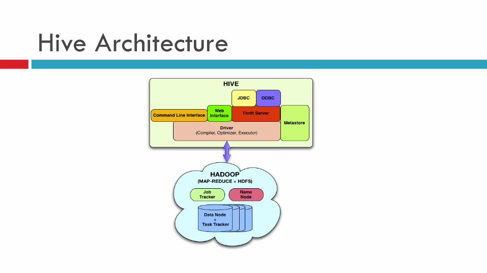
Hive Architecture
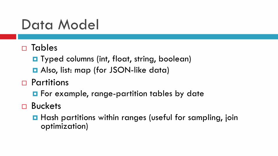
Data Model ¨ Tables
¤ Typed columns (int, float, string, boolean) ¤ Also, list: map (for JSON-like data)
¨ Partitions ¤ For example, range-partition tables by date
¨ Buckets ¤ Hash partitions within ranges (useful for sampling, join
optimization)
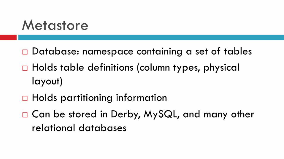
Metastore ¨ Database: namespace containing a set of tables ¨ Holds table definitions (column types, physical
layout) ¨ Holds partitioning information ¨ Can be stored in Derby, MySQL, and many other
relational databases
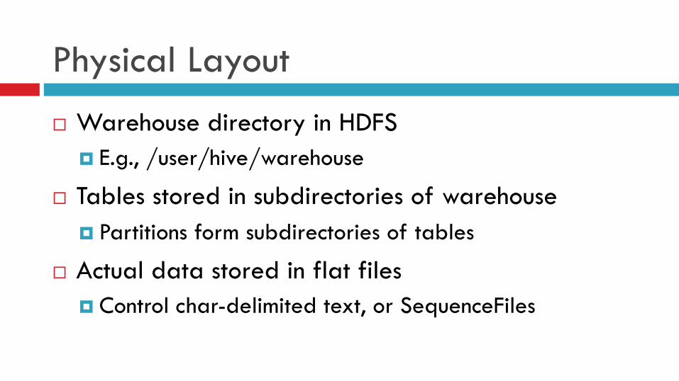
Physical Layout ¨ Warehouse directory in HDFS
¤ E.g., /user/hive/warehouse
¨ Tables stored in subdirectories of warehouse ¤ Partitions form subdirectories of tables
¨ Actual data stored in flat files ¤ Control char-delimited text, or SequenceFiles
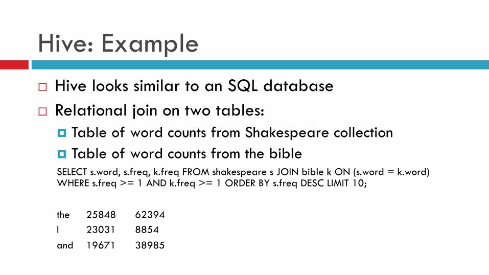
Hive: Example ¨ Hive looks similar to an SQL database ¨ Relational join on two tables:
¤ Table of word counts from Shakespeare collection ¤ Table of word counts from the bible SELECT s.word, s.freq, k.freq FROM shakespeare s JOIN bible k ON (s.word = k.word) WHERE s.freq >= 1 AND k.freq >= 1 ORDER BY s.freq DESC LIMIT 10; the 25848 62394 I 23031 8854 and 19671 38985
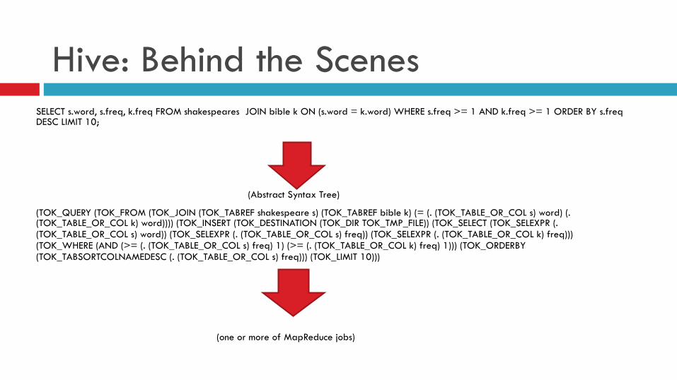
Hive: Behind the Scenes SELECT s.word, s.freq, k.freq FROM shakespeares JOIN bible k ON (s.word = k.word) WHERE s.freq >= 1 AND k.freq >= 1 ORDER BY s.freq DESC LIMIT 10;
(TOK_QUERY (TOK_FROM (TOK_JOIN (TOK_TABREF shakespeare s) (TOK_TABREF bible k) (= (. (TOK_TABLE_OR_COL s) word) (. (TOK_TABLE_OR_COL k) word)))) (TOK_INSERT (TOK_DESTINATION (TOK_DIR TOK_TMP_FILE)) (TOK_SELECT (TOK_SELEXPR (. (TOK_TABLE_OR_COL s) word)) (TOK_SELEXPR (. (TOK_TABLE_OR_COL s) freq)) (TOK_SELEXPR (. (TOK_TABLE_OR_COL k) freq))) (TOK_WHERE (AND (>= (. (TOK_TABLE_OR_COL s) freq) 1) (>= (. (TOK_TABLE_OR_COL k) freq) 1))) (TOK_ORDERBY (TOK_TABSORTCOLNAMEDESC (. (TOK_TABLE_OR_COL s) freq))) (TOK_LIMIT 10)))
(one or more of MapReduce jobs)
(Abstract Syntax Tree)

Hive: Behind the Scenes
Hive - Installation ¨ Pre-Request
¤ Hadoop is installed ¤ HDFS is available
¨ Download hive ¨ Extract Hive ¨ Configure Hive

Hive - Setup tar – xvf hive-0.8.1-bin cd hive-0.8.1-bin/ export HIVE_HOME=/home/guest/hive-0.8.1-bin export PATH=/home/guest/hive-0.8.1-bin/bin/:$PATH export PATH=/home/guest/hadoop/bin/:$PATH Check Hadoop is in path developer@ubuntu:~/hive-0.8.1-bin$ hadoop fs -ls Found 2 items drwxr-xr-x - developer supergroup 0 2011-06-02 04:01 /user/developer/input drwxr-xr-x - developer supergroup 0 2011-06-16 02:12 /user/developer/output
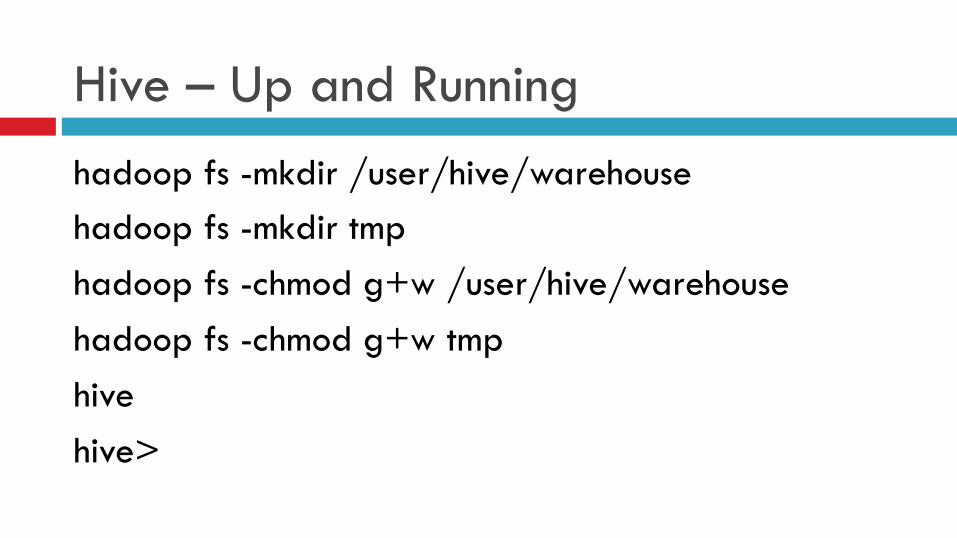
Hive – Up and Running hadoop fs -mkdir /user/hive/warehouse hadoop fs -mkdir tmp hadoop fs -chmod g+w /user/hive/warehouse hadoop fs -chmod g+w tmp hive hive>
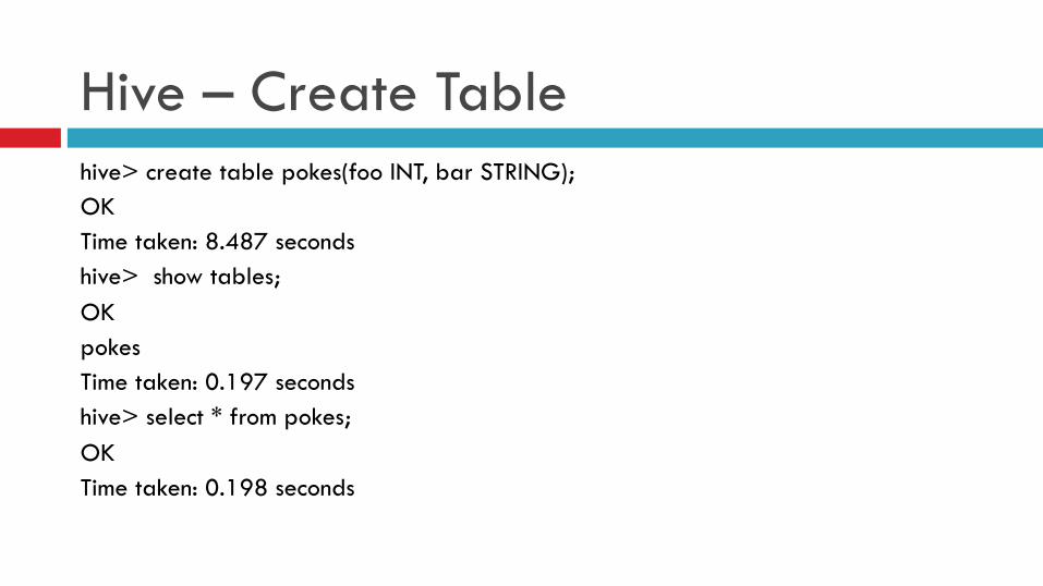
Hive – Create Table hive> create table pokes(foo INT, bar STRING); OK Time taken: 8.487 seconds hive> show tables; OK pokes Time taken: 0.197 seconds hive> select * from pokes; OK Time taken: 0.198 seconds
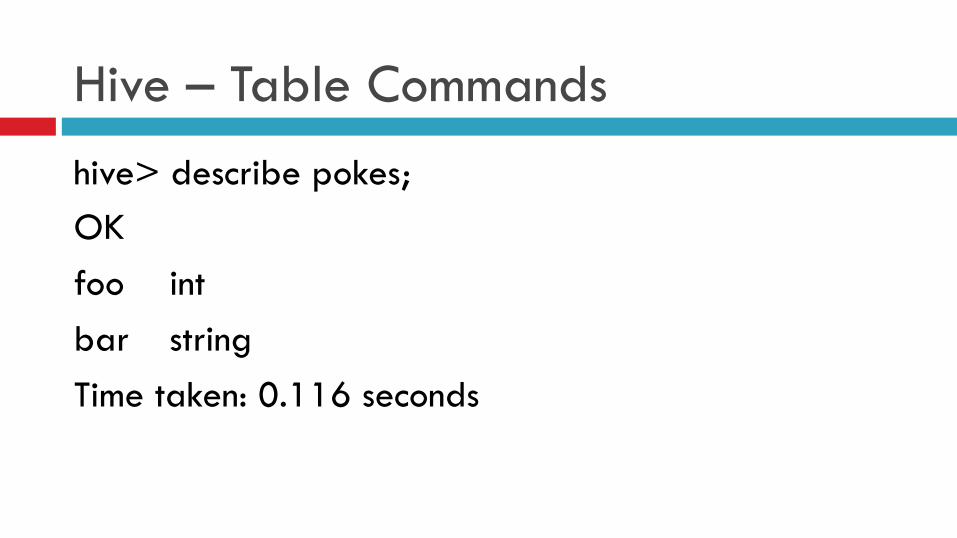
Hive – Table Commands hive> describe pokes; OK foo int bar string Time taken: 0.116 seconds
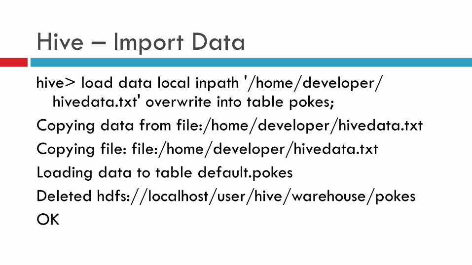
Hive – Import Data hive> load data local inpath '/home/developer/
hivedata.txt' overwrite into table pokes; Copying data from file:/home/developer/hivedata.txt Copying file: file:/home/developer/hivedata.txt Loading data to table default.pokes Deleted hdfs://localhost/user/hive/warehouse/pokes OK
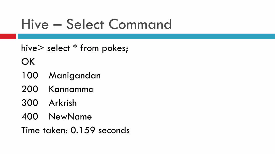
Hive – Select Command hive> select * from pokes; OK 100 Manigandan 200 Kannamma 300 Arkrish 400 NewName Time taken: 0.159 seconds
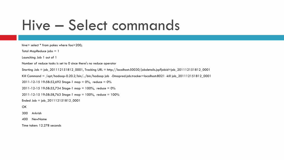
Hive – Select commands hive> select * from pokes where foo>200;
Total MapReduce jobs = 1
Launching Job 1 out of 1
Number of reduce tasks is set to 0 since there's no reduce operator
Starting Job = job_201112151812_0001, Tracking URL = http://localhost:50030/jobdetails.jsp?jobid=job_201112151812_0001
Kill Command = /opt/hadoop-0.20.2/bin/../bin/hadoop job -Dmapred.job.tracker=localhost:8021 -kill job_201112151812_0001
2011-12-15 19:58:52,692 Stage-1 map = 0%, reduce = 0%
2011-12-15 19:58:55,734 Stage-1 map = 100%, reduce = 0%
2011-12-15 19:58:58,763 Stage-1 map = 100%, reduce = 100%
Ended Job = job_201112151812_0001
OK
300 Arkrish
400 NewName
Time taken: 12.278 seconds
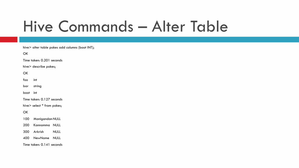
Hive Commands – Alter Table hive> alter table pokes add columns (boot INT);
OK
Time taken: 0.201 seconds
hive> describe pokes;
OK
foo int
bar string
boot int
Time taken: 0.127 seconds
hive> select * from pokes;
OK
100 Manigandan NULL
200 Kannamma NULL
300 Arkrish NULL
400 NewName NULL
Time taken: 0.141 seconds
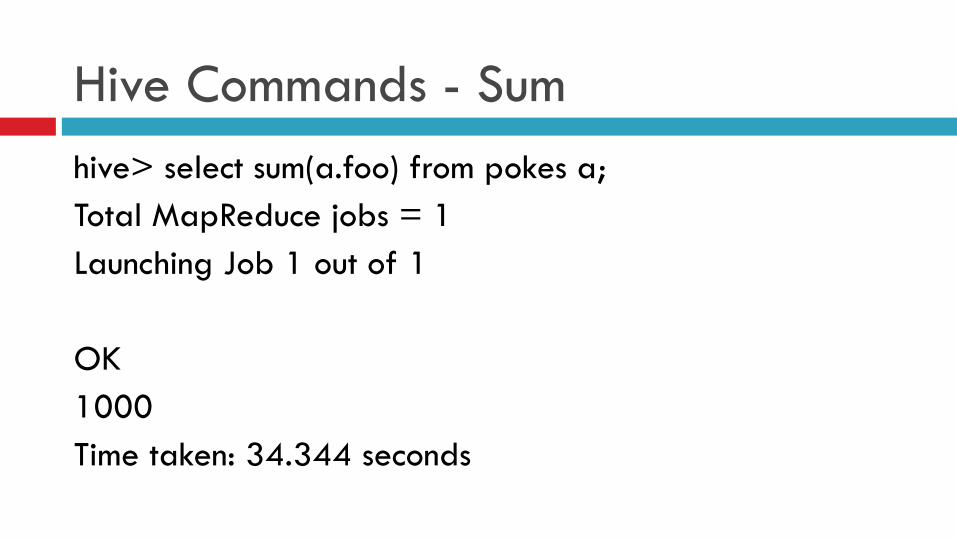
Hive Commands - Sum hive> select sum(a.foo) from pokes a; Total MapReduce jobs = 1 Launching Job 1 out of 1 OK 1000 Time taken: 34.344 seconds
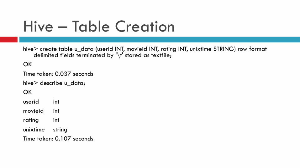
Hive – Table Creation hive> create table u_data (userid INT, movieid INT, rating INT, unixtime STRING) row format
delimited fields terminated by '\t' stored as textfile; OK Time taken: 0.037 seconds hive> describe u_data; OK userid int movieid int rating int unixtime string Time taken: 0.107 seconds
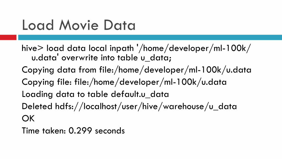
Load Movie Data hive> load data local inpath '/home/developer/ml-100k/
u.data' overwrite into table u_data; Copying data from file:/home/developer/ml-100k/u.data Copying file: file:/home/developer/ml-100k/u.data Loading data to table default.u_data Deleted hdfs://localhost/user/hive/warehouse/u_data OK Time taken: 0.299 seconds
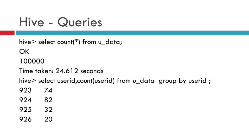
Hive - Queries hive> select count(*) from u_data; OK 100000 Time taken: 24.612 seconds hive> select userid,count(userid) from u_data group by userid ; 923 74 924 82 925 32 926 20
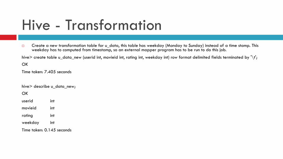
Hive - Transformation ¨ Create a new transformation table for u_data, this table has weekday (Monday to Sunday) instead of a time stamp. This
weekday has to computed from timestamp, so an external mapper program has to be run to do this job.
hive> create table u_data_new (userid int, movieid int, rating int, weekday int) row format delimited fields terminated by '\t';
OK
Time taken: 7.405 seconds
hive> describe u_data_new;
OK
userid int
movieid int
rating int
weekday int
Time taken: 0.145 seconds
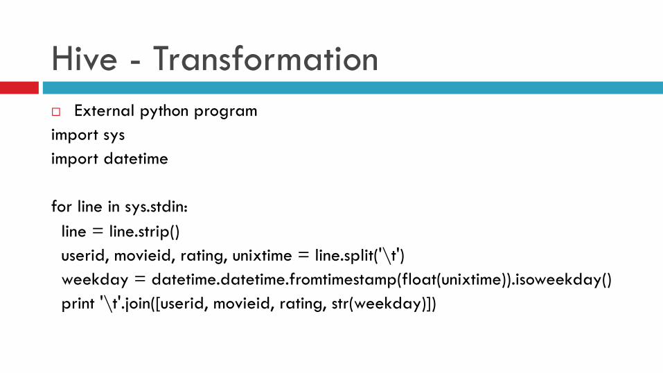
Hive - Transformation ¨ External python program import sys import datetime for line in sys.stdin: line = line.strip() userid, movieid, rating, unixtime = line.split('\t') weekday = datetime.datetime.fromtimestamp(float(unixtime)).isoweekday() print '\t'.join([userid, movieid, rating, str(weekday)])
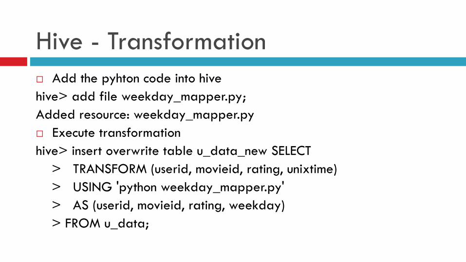
Hive - Transformation ¨ Add the pyhton code into hive hive> add file weekday_mapper.py; Added resource: weekday_mapper.py ¨ Execute transformation hive> insert overwrite table u_data_new SELECT > TRANSFORM (userid, movieid, rating, unixtime) > USING 'python weekday_mapper.py' > AS (userid, movieid, rating, weekday) > FROM u_data;
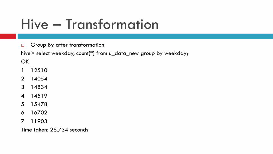
Hive – Transformation ¨ Group By after transformation hive> select weekday, count(*) from u_data_new group by weekday; OK 1 12510 2 14054 3 14834 4 14519 5 15478 6 16702 7 11903 Time taken: 26.734 seconds
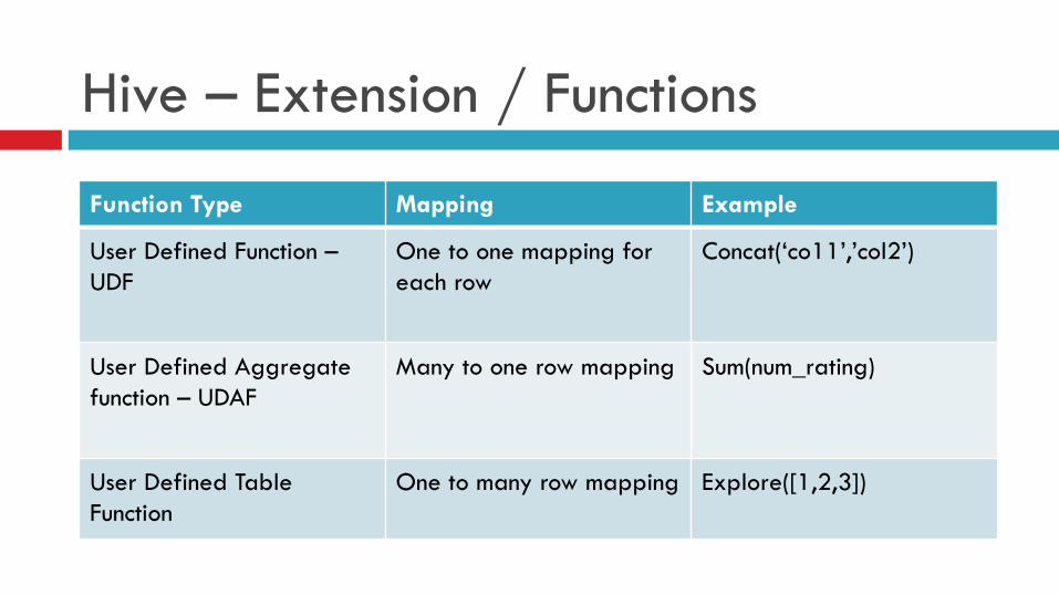
Hive – Extension / Functions
Function Type Mapping Example
User Defined Function – UDF
One to one mapping for each row
Concat(‘co11’,’col2’)
User Defined Aggregate function – UDAF
Many to one row mapping Sum(num_rating)
User Defined Table Function
One to many row mapping Explore([1,2,3])
Hive – SQL Query ¨ select distinct userid from u_data;
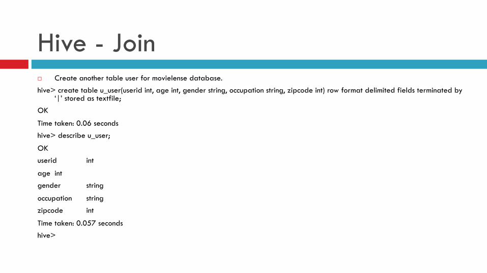
Hive - Join ¨ Create another table user for movielense database.
hive> create table u_user(userid int, age int, gender string, occupation string, zipcode int) row format delimited fields terminated by ‘|’ stored as textfile;
OK
Time taken: 0.06 seconds
hive> describe u_user;
OK
userid int
age int
gender string
occupation string
zipcode int
Time taken: 0.057 seconds
hive>
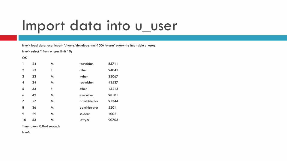
Import data into u_user hive> load data local inpath '/home/developer/ml-100k/u.user' overwrite into table u_user;
hive> select * from u_user limit 10;
OK
1 24 M technician 85711
2 53 F other 94043
3 23 M writer 32067
4 24 M technician 43537
5 33 F other 15213
6 42 M executive 98101
7 57 M administrator 91344
8 36 M administrator 5201
9 29 M student 1002
10 53 M lawyer 90703
Time taken: 0.064 seconds
hive>
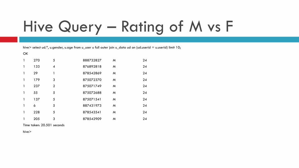
Hive Query – Rating of M vs F hive> select ud.*, u.gender, u.age from u_user u full outer join u_data ud on (ud.userid = u.userid) limit 10;
OK
1 270 5 888732827 M 24
1 133 4 876892818 M 24
1 29 1 878542869 M 24
1 179 3 875072370 M 24
1 237 2 875071749 M 24
1 55 5 875072688 M 24
1 137 5 875071541 M 24
1 6 5 887431973 M 24
1 228 5 878543541 M 24
1 205 3 878542909 M 24
Time taken: 20.501 seconds
hive>
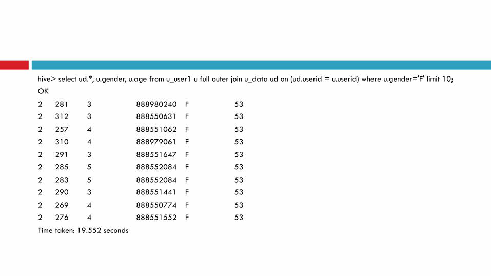
hive> select ud.*, u.gender, u.age from u_user1 u full outer join u_data ud on (ud.userid = u.userid) where u.gender='F' limit 10;
OK
2 281 3 888980240 F 53
2 312 3 888550631 F 53
2 257 4 888551062 F 53
2 310 4 888979061 F 53
2 291 3 888551647 F 53
2 285 5 888552084 F 53
2 283 5 888552084 F 53
2 290 3 888551441 F 53
2 269 4 888550774 F 53
2 276 4 888551552 F 53
Time taken: 19.552 seconds
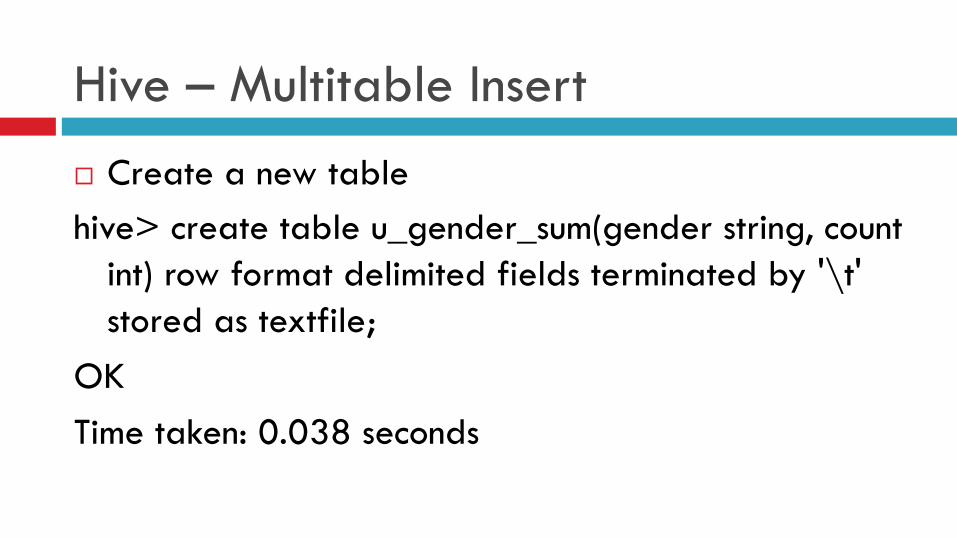
Hive – Multitable Insert ¨ Create a new table hive> create table u_gender_sum(gender string, count
int) row format delimited fields terminated by '\t' stored as textfile;
OK Time taken: 0.038 seconds
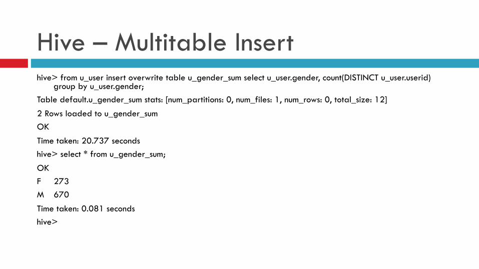
Hive – Multitable Insert hive> from u_user insert overwrite table u_gender_sum select u_user.gender, count(DISTINCT u_user.userid)
group by u_user.gender; Table default.u_gender_sum stats: [num_partitions: 0, num_files: 1, num_rows: 0, total_size: 12]
2 Rows loaded to u_gender_sum OK
Time taken: 20.737 seconds hive> select * from u_gender_sum;
OK F 273 M 670
Time taken: 0.081 seconds hive>
Apache Pig
Apache Pig- Rationale ¨ Innovation is driven by ad-hoc analysis of large
data sets ¨ Parallelism is needed to analyze large datasets ¨ Programming in cluster computing is difficult and
time- consuming ¨ Pig makes it easy to harness the power of cluster
computing for ad-hoc data analysis
What is Pig ¨ Pig compiles data analysis tasks into Map-Reduce
jobs and runs them on Hadoop ¨ Pig Latin is a language for expressing data
transformation flows ¨ Pig can be made to understand other languages,
too
Apache Pig ¨ Apache Pig is a platform for analyzing large data sets that consists of a high-level
language for expressing data analysis programs, coupled with infrastructure for evaluating these programs.
¨ Pig's infrastructure layer consists of ¤ a compiler that produces sequences of Map-Reduce programs, ¤ Pig's language layer currently consists of a textual language called Pig Latin, which has
the following key properties: n Ease of programming. It is trivial to achieve parallel execution of simple, "embarrassingly parallel"
data analysis tasks. Complex tasks comprised of multiple interrelated data transformations are explicitly encoded as data flow sequences, making them easy to write, understand, and maintain.
n Optimization opportunities. The way in which tasks are encoded permits the system to optimize their execution automatically, allowing the user to focus on semantics rather than efficiency.
n Extensibility. Users can create their own functions to do special-purpose processing.
Sawzall Vs. Pig ¨ Sawzall from Google
¤ Fairly rigid structure consisting of a filtering phase (the map step) ¤ followed by an aggregation phase (the reduce step) ¤ Only the filtering phase can be written by the user, and only a pre-built set of
aggregations are available (new ones are non-trivial to add) ¨ •Pig Latin fromYahoo
¤ Has similar higher level primitives like filtering and aggregation, an arbitrary number of them can be flexibly chained together in a Pig Latin program
¤ Additional primitives such as cogrouping, that allow operations such as joins ¤ Pig Latin is designed to be embedded into other languages, and can use
functions written in other languages

SQL Vs. Pig ¨ SQL requires
¤ Import data into database’s internal format ¤ Well-structured, normalized data with a declared schema ¤ Programs expressed in declarative SELECT-FROM-WHERE blocks
¨ Pig Latin facilitates ¤ Interoperability - i.e. data may be read/written in a format accepted by ¤ other applications such as text editors or graph generators ¤ flexibility, i.e. data may be loosely structured or have structure that is defined
operationally ¤ adoption by programmers who find procedural programming more natural than
declarative programming
Getting started with Pig ¨ Installing and using Pig it is extremely easy ¨ Download the tar, untar and add it in your PATH ¨ You can execute Pig Latin statements:
¤ Using grunt shell or command line $ pig ... - Connecting to ... grunt> A = load 'data'; grunt> B = ... ;
¤ In local mode or hadoop mapreduce mode $ pig myscript.pig Command Line - batch, local mode mode $ pig -x local myscript.pig
¨ Either interactively or in batch • Easy,isn'tit?
Program/flow organization ¨ A LOAD statement reads data from the file system. ¨ A series of "transformation" statements process the
data. ¨ A STORE statement writes output to the file system;
or, a DUMP statement displays output to the screen.
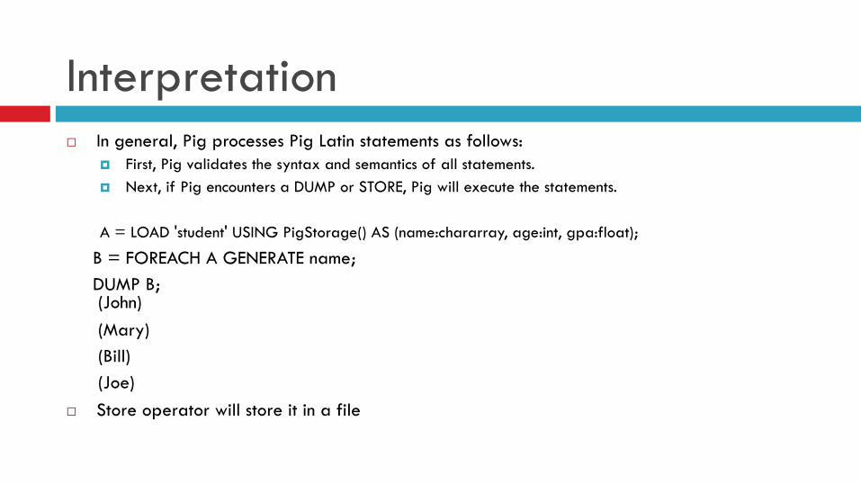
Interpretation ¨ In general, Pig processes Pig Latin statements as follows:
¤ First, Pig validates the syntax and semantics of all statements. ¤ Next, if Pig encounters a DUMP or STORE, Pig will execute the statements.
A = LOAD 'student' USING PigStorage() AS (name:chararray, age:int, gpa:float);
B = FOREACH A GENERATE name; DUMP B; (John) (Mary) (Bill) (Joe) ¨ Store operator will store it in a file
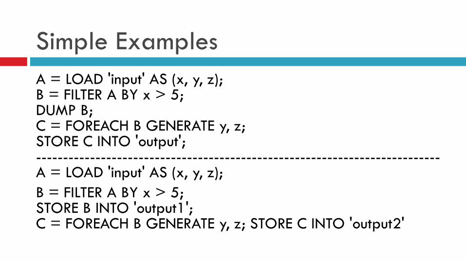
Simple Examples A = LOAD 'input' AS (x, y, z); B = FILTER A BY x > 5; DUMP B; C = FOREACH B GENERATE y, z; STORE C INTO 'output'; ---------------------------------------------------------------------------A = LOAD 'input' AS (x, y, z); B = FILTER A BY x > 5; STORE B INTO 'output1'; C = FOREACH B GENERATE y, z; STORE C INTO 'output2'
Relations, Bags, Tuples, Fields ¨ Pig Latin statements work with relations. ¨ A relation can be defined as:
¤ A relation is a bag (more specifically, an outer bag). ¤ A bag is a collection of tuples. ¤ A tuple is an ordered set of fields. ¤ A field is a piece of data.
Language Features ¨ FILTER, FOREACH GENERATE, GROUP BY, UNION, DISTINCT, ORDER
BY, SAMPLE, JOIN, ... ¨ AVG, CONCAT, COUNT, MAX, MIN, SUM, TOKENZIE, regex tools,
math stuff, ... ¨ HDFS manipulation ¨ Shell access ¨ Streaming ¨ MapReduce Streaming ¨ UDFs
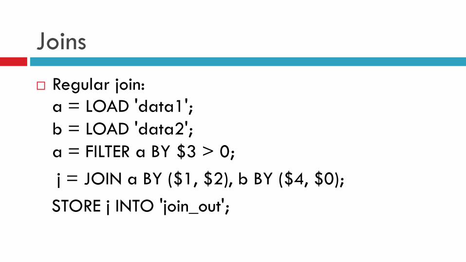
Joins ¨ Regular join:
a = LOAD 'data1'; b = LOAD 'data2'; a = FILTER a BY $3 > 0;
j = JOIN a BY ($1, $2), b BY ($4, $0); STORE j INTO 'join_out';
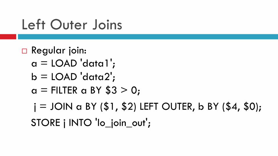
Left Outer Joins ¨ Regular join:
a = LOAD 'data1'; b = LOAD 'data2'; a = FILTER a BY $3 > 0;
j = JOIN a BY ($1, $2) LEFT OUTER, b BY ($4, $0); STORE j INTO 'lo_join_out';
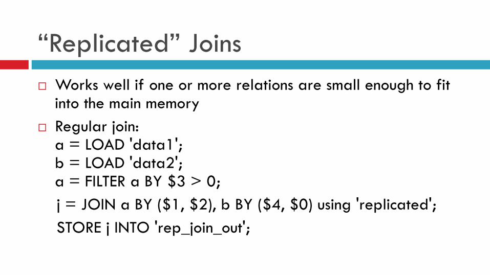
“Replicated” Joins ¨ Works well if one or more relations are small enough to fit
into the main memory ¨ Regular join:
a = LOAD 'data1'; b = LOAD 'data2'; a = FILTER a BY $3 > 0;
j = JOIN a BY ($1, $2), b BY ($4, $0) using 'replicated'; STORE j INTO 'rep_join_out';
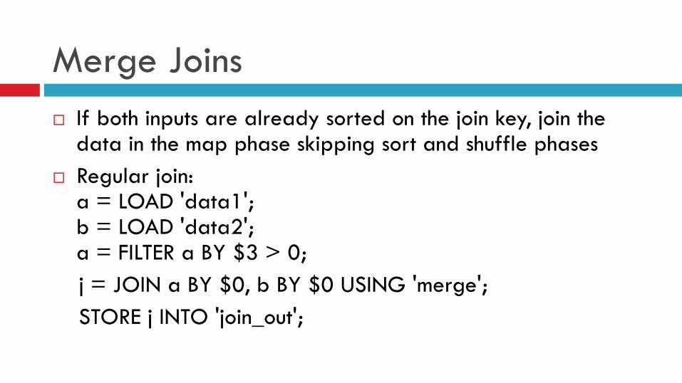
Merge Joins ¨ If both inputs are already sorted on the join key, join the
data in the map phase skipping sort and shuffle phases ¨ Regular join:
a = LOAD 'data1'; b = LOAD 'data2'; a = FILTER a BY $3 > 0;
j = JOIN a BY $0, b BY $0 USING 'merge'; STORE j INTO 'join_out';