habitat selection and movement patterns of …
TRANSCRIPT

HABITAT SELECTION AND MOVEMENT PATTERNS OF AMPHIBIANS IN ALTERED
FOREST HABITATS
by
GABRIELLE JOY GRAETER
(Under the Direction of J. WHITFIELD GIBBONS)
ABSTRACT
I released adult southern leopard frogs (Rana sphenocephala), marbled salamanders (Ambystoma
opacum), and southern toads (Bufo terrestris) on forest/clearcut edges to examine the effects of forest
management on amphibian habitat selection and movement behavior. Salamanders selected habitat at
random, toads preferred clearcuts, and frogs initially selected clearcuts but ultimately chose forests. All
three species made more turns in clearcuts than forests, and toads and frogs moved farther in forests.
Frogs and toads moved without regard to environmental conditions, but salamanders were influenced by
soil moisture. I also examined the efficacy of fluorescent powder as an amphibian tracking technique and
found that some colors were easier to detect when paths were long, that heavy rainfall truncated path
length, and that effectiveness varied among species, habitat, and region. Such knowledge of individual
and species-level responses to terrestrial habitat alteration will facilitate development of forest
management plans that enhance persistence of amphibian populations.
INDEX WORDS: Ambystoma opacum, Bufo terrestris, Rana sphenocephala, marbled salamander, southern toad, southern leopard frog, habitat fragmentation, forest management, amphibians, movement, migration, habitat selection, permeability, fluorescent powder, tracking, clearcut, amphibian conservation

HABITAT SELECTION AND MOVEMENT PATTERNS OF AMPHIBIANS IN ALTERED
FOREST HABITATS
by
GABRIELLE JOY GRAETER
B.S., University of North Carolina-Chapel Hill, 1999
A Thesis Submitted to the Graduate Faculty of The University of Georgia in Partial Fulfillment
of the Requirements for the Degree
MASTER OF SCIENCE
ATHENS, GEORGIA
2005

© 2005
Gabrielle Joy Graeter
All Rights Reserved

HABITAT SELECTION AND MOVEMENT PATTERNS OF AMPHIBIANS IN ALTERED
FOREST HABITATS
by
GABRIELLE JOY GRAETER
Major Professor: J. Whitfield Gibbons
Committee: Mary C. Freeman C. Ronald Carroll Betsie B. Rothermel
Electronic Version Approved: Maureen Grasso Dean of the Graduate School The University of Georgia December 2005

iv
ACKNOWLEDGEMENTS
I thank Whit Gibbons for his constant encouragement, support, and dedication to his students. I
feel honored to be one of Whit’s students and am inspired by his incredible amount of energy and
enthusiasm for herpetology and education. I thank Betsie Rothermel for her continual guidance and help
with all stages of my research and thesis. She provided invaluable support and information and I am very
grateful for her mentorship.
I also thank Mary Freeman, especially for her guidance during my on-campus year and her
willingness to assist me with statistical dilemmas. I thank Ron Carroll for his support and in helping me
to look at my research from a broader perspective.
Many others have helped me, with field work, statistics, advice, or other support. I could not
have accomplished this without their generosity: Kimberly Andrews, David Berry, Sean Blomquist,
Chris Conner, Sarah Durant, Aaliyah Green, Judy Greene-McLeod, Deno Karapatakis, Mark Langley,
Tom Luhring, Brian Metts, John Nestor, Leslie Ruyle, Brian Todd, Tracey Tuberville, JD Willson,
Machelle Wilson, Chris Winne, Meredith Wright, and Leslie Zorn. I also want to thank my parents, John
and Kathryn Graeter, brother and sister, Jesse Graeter and Amanda Miles-Graeter, and grandparents,
Harry and Bess Wehrlen, for their love and encouragement.

v
TABLE OF CONTENTS
Page
ACKNOWLEDGEMENTS........................................................................................................... iv
LIST OF TABLES........................................................................................................................ vii
LIST OF FIGURES ..................................................................................................................... viii
CHAPTER
1 INTRODUCTION AND LITERATURE REVIEW .....................................................1
Background on Amphibian Ecology and Conservation Issues .................................1
Forest Management in the Southeast.........................................................................3
Summary of Previous Research on Amphibian Responses to Forest Management..5
Amphibian Population-Level Responses to Forest Management in the Southeastern
Coastal Plain..............................................................................................................6
Movement Responses of Individual Amphibians to Forest Management ................7
Objectives of Study .................................................................................................14
Literature Cited........................................................................................................15
2 HABITAT SELECTION AND MOVEMENT PATTERNS OF THREE
AMPHIBIAN SPECIES (RANA SPHENOCEPHALA, AMBYSTOMA
OPACUM, BUFO TERRESTRIS) IN ALTERED FOREST HABITATS IN THE
UPPER COASTAL PLAIN OF SOUTH CAROLINA ..........................................20
Introduction .............................................................................................................21
Materials and Methods ............................................................................................23

vi
Results .....................................................................................................................34
Discussion ...............................................................................................................38
Conclusions and Implications .................................................................................49
Acknowledgements .................................................................................................54
Literature Cited........................................................................................................55
3 THE USE OF FLUORESCENT POWDERED PIGMENTS AS AN EFFECTIVE
TECHNIQUE FOR TRACKING AMPHIBIANS..................................................78
Introduction .............................................................................................................79
Materials and Methods ............................................................................................80
Results .....................................................................................................................81
Discussion ...............................................................................................................82
Acknowledgements .................................................................................................85
Literature Cited........................................................................................................86
4 CONCLUSION............................................................................................................91

vii
LIST OF TABLES
Page
Table 2.1: Binomial probability results for R. sphenocephala, A. opacum, and B. terrestris by
edge type........................................................................................................................62
Table 2.2: Binomial probability results for R. sphenocephala, A. opacum, and B. terrestris, with
data condensed into two treatments, Forest v. Clearcut ...............................................63
Table 2.3: Results of multivariate analysis of variance of the effects of treatment, site, and their
interaction on each species’ movement path characteristics .........................................63
Table 2.4: Ground-level openness candidate models showing fixed effects, model ∆i values, and
Akaike weights ..............................................................................................................64
Table 2.5: Fixed effects coefficient estimates for the highest ranked models for each composite
variable ..........................................................................................................................64
Table 2.6: Ground-level cover candidate models showing fixed effects, model ∆i values, and
Akaike weights ..............................................................................................................65
Table 2.7: Tree density candidate models showing fixed effects, model ∆i values, and Akaike
weights...........................................................................................................................65

viii
LIST OF FIGURES
Page
Figure 2.1: Diagram of a LEAP array showing the arrangement of the four forest management
treatments ......................................................................................................................66
Figure 2.2: Diagram of microhabitat availability transects in one quadrant..................................66
Figure 2.3: Percentage of R. sphenocephala in clearcut v. forest at selected distances from the
release point on forest/clearcut edges............................................................................67
Figure 2.4: Percentage of A. opacum in clearcut v. forest at 2 m and endpoint from the release
point on forest/clearcut edges........................................................................................67
Figure 2.5: Percentage of B. terrestris in clearcut v. forest at 5 m and endpoint from the release
point on forest/clearcut edges........................................................................................68
Figure 2.6: Movement paths of R. sphenocephala at (A) site 1000 and (B) site 37......................69
Figure 2.7: Movement paths of B. terrestris at (A) site 37 and (B) site 119 .................................70
Figure 2.8: Movement paths of A. opacum at (A) site 119 and (B) site 37 ...................................71
Figure 2.8C: A close-up of the A. opacum movement paths on the control/CC-removed edge at
site 37 ............................................................................................................................72
Figure 2.9: Mean path length for each species ..............................................................................73
Figure 2.10: Minimum and maximum path lengths for each species ............................................73
Figure 2.11: Mean number of turns per 10 m for each species......................................................74
Figure 2.12: Mean path linearity for each species .........................................................................74
Figure 2.13: Mean path length in forests v. clearcuts for each species .........................................75

ix
Figure 2.14: Mean number of turns per 10 m in forests v. clearcuts for each species...................75
Figure 2.15: Mean path linearity in forests v. clearcuts for each species ......................................76
Figure 2.16: Mean values for ground-level openness availability v. ground-level openness use by
R. sphenocephala by treatment type and site ................................................................76
Figure 2.17: Mean values for ground-level cover availability v. ground-level cover use by R.
sphenocephala by treatment type and site.....................................................................77
Figure 2.18: Mean values for tree density availability v. tree density use by R. sphenocephala by
treatment type and site...................................................................................................77
Figure 3.1: Mean, minimum, maximum path lengths of A. opacum, B. terrestris, and R.
sphenocephala in S.C. (this study), A. annulatum in M.O., and R. sylvatica in M.E. ..88
Figure 3.2: Mean path length for the four fluorescent powder colors ...........................................89
Figure 3.3: Mean path length for powder color, specific to species ..............................................89
Figure 3.4: Relationship between post-release precipitation and mean and maximum powder path
length in (A) R. sphenocephala at three different precipitation levels and (B) in A.
opacum at two different precipitation levels ................................................................90

1
CHAPTER 1
INTRODUCTION AND LITERATURE REVIEW
Background on Amphibian Ecology and Conservation Issues
Place in Ecosystems
Amphibians are an important group of organisms for many reasons, including their role in
transferring energy and nutrients between terrestrial and aquatic habitats, their high abundances in some
areas, their integral role in food webs, and their usefulness as biological indicators of environmental
degradation. Through the use of both terrestrial and aquatic habitats, as they move between the two for
reproduction and in search of suitable habitat, many amphibians effectively transport nutrients and energy
between the two environments (Wilbur 1980, Gibbons et al. in press). This transfer can have huge
implications for the productivity and nutrient cycles of the adjoining habitats and for the survival and
reproduction of other species within the food web (Wilbur 1980). Studies, both classic and recent, have
shown that amphibians occur in remarkably high abundances in some areas (Burton and Likens 1975,
Hairston 1987, Petranka and Murray 2001, Gibbons et al. in press). When amphibians exist in high
biomass, it follows that they would play important ecosystem roles by providing a large amount of prey
and nutrients to that particular locale (Petranka and Murray 2001). On a related note, amphibians are a
critical link in many food webs because they provide a prey source for a wide variety of vertebrates
including birds, snakes, mammals, and fish (Hairston 1987), and because they prey on invertebrates and
other food items that are too small for many other organisms (Pough 1983). Lastly, their sensitivity to
environmental changes renders amphibians particularly suitable as biological indicators of environmental
health and integrity (Dunson et al. 1992, Blaustein 1994).

2
Habitat Use and Ecology
Most amphibians have biphasic life cycles and rely on both aquatic and terrestrial habitats during
some portion of their life (Pough 2004). As ectotherms with highly permeable skin, amphibians usually
have body temperatures that mirror their immediate surroundings; thus, they must adjust their behavior
accordingly to regulate their body temperature and hydration levels (Duellman and Trueb 1994, Kam and
Chen 2000). Not only do amphibians need adequate unaltered habitat, they also require specific habitat
types at different life stages.
The United States has a diversity of isolated wetland types, including Carolina bays, cypress
domes, desert wetlands, floodplain wetlands, karst wetlands, kettle-hole bogs, playas, pocosins, prairie
potholes, sinkhole wetlands, and vernal pools (Tiner 2003). Many in the southeastern Coastal Plain are
depression wetlands that fill from rainfall and dry seasonally. These ephemeral wetlands are particularly
important for amphibian reproduction because the process of periodic drying and subsequent inundation
excludes fish, which are significant predators on amphibian eggs and larvae (Semlitsch 2000, Teplitsky et
al. 2003). The small size of these wetlands should not imply that they are less important; in fact, these
small wetlands can be centers of great productivity and biodiversity (Russell et al. 2002a, Gibbons et al.
in press).
However, as critical as these wetlands are, the time spent in these aquatic habitats is only a small
portion of most amphibians’ life cycles because the majority of time is spent in the terrestrial landscapes
surrounding these wetlands (Semlitsch 1998, Gibbons 2003). Most amphibians that use these wetlands
only return to breed and many species will skip breeding in years when conditions are not suitable for
reproduction (Bailey et al. 2004). Recently, numerous studies have emphasized the significance of the
terrestrial component of amphibian life cycles and the necessity of protecting both the aquatic and
terrestrial habitats (Gibbons 2003, Semlitsch and Bodie 2003, Porej et al. 2004). Information has been
compiled for individual species on terrestrial habitat needs, and several alternative strategies for
protection of terrestrial buffers around wetlands have been suggested as means to protect amphibians
from environmental threats (Bulger et al. 2003, Semlitsch and Bodie 2003, Schabetsberger et al. 2004).

3
Conservation Status
Amphibian populations are declining worldwide (Blaustein et al. 1994, Gibbons et al. 2000,
Stuart et al. 2004) and these declines are attributed to many different causes, including introduced exotic
species, disease, ultraviolet radiation, and environmental contaminants (Blaustein and Kiesecker 2002).
Although these causes are probably interacting synergistically, habitat degradation and loss is considered
by most amphibian ecologists to be the primary cause of these declines (Alford and Richards 1999).
Amphibians are facing these same threats in the southeastern United States (Means et al. 1996). While
large-scale amphibian population crashes have not yet occurred in the Southeast as they have elsewhere,
many species are considered to be declining or at risk (Dodd 1997, Means 2005). In fact, of the 77
amphibian species native to the Coastal Plain, 15 (19%) have been ranked G-1 (critically imperiled) to G-
4 (apparently secure, but not demonstrably widespread, abundant, and secure) by The Nature
Conservancy (Means 2005).
It seems apparent that as the pressures and consequences of human population growth escalate,
amphibians in the Southeast will be increasingly more at risk unless positive changes are made. Between
2000 and 2004, human population has increased by 6.6% in the South Atlantic states and by 4.6% in
South Carolina (U.S. Census Bureau 2004). This rate of human population increase is predicted to result
in greater rates of urbanization (Wear 2002) and an intensification of forest management and productivity
on existing timberland (Prestemon and Abt 2002).
Forest Management in the Southeast
According to a report by the United States Forest Service (Prestemon and Abt 2002), the
Southeast produces more timber than any single country in the world and produces about 60 percent of
the timber products in the United States, almost all of which is from privately owned forests. The
Southeast is projected to retain this status for decades to come (Prestemon and Abt 2002). In fact, prices
for timber are expected to increase over the next 40 years, and this is anticipated to serve as an incentive
to private timber companies to improve their productivity and invest in more intensive forest management

4
(Prestemon and Abt 2002). The amount of land in the South managed as pine plantations is projected to
increase continuously, resulting in a 67 percent increase (from 33 to 54 million acres) over a 45 year
period, between 1995 and 2040 (Prestemon and Abt 2002).
Forest management for timber production is not only a prevalent practice throughout the
southeastern United States, it is also of considerable importance to the economy. In 1997, the direct
overall economic gain from the different sectors of the timber industry (includes timber, logging,
sawmills, wood furniture, pulp and paper, and all other wood products) in the South was more than $40
million (Abt et al. 2002). In the same year, the wood products sectors contributed over 770,000 direct
jobs to the southern economy, $120 billion in total industry output, and over $40 billion in Gross
Regional Product (Abt et al. 2002).
Although the management methods vary within the different regions in the Southeast, the
majority of timber production in the Coastal Plain is derived from a combination of pine plantations and
mixed hardwood stands (Conner and Hartsell 2002). Throughout the lower Coastal Plain, loblolly (Pinus
taeda) and short-leaf pine (Pinus echinata) are the predominant species in planted pine forests (15 million
acres), with a lesser amount (12.5 million acres) planted in slash (Pinus elliottii) and long-leaf pine (Pinus
palustris, Conner and Hartsell 2002). In addition, oak-pine (8.2 million acres), oak-hickory (8.9 million
acres), and oak-gum-cypress (13.9 million acres) forests make up a major portion of managed Coastal
Plain forests (Conner and Hartsell 2002).
The timber industry in South Carolina typically mirrors the overall trends in the Southeast.
Between 1952 and 1999, South Carolina experienced a large increase in the area of planted pine forests
(from 233,000 to 2.7 million acres) and a simultaneous decrease in land area with natural pine forests
(from 5.9 million to 2.8 million acres, Conner and Hartsell 2002). In fact, a recent inventory discovered
that more land in South Carolina is planted in pine plantations than natural pine forests; as of 2001, the
3.1 million acres of planted pine stands outnumbered natural pine by 150,000 acres (Conner et al. 2004).
One pine species, loblolly pine, made up 94 percent of pine plantation acres as of 2001 (Conner et al.
2004). In terms of economic input, South Carolina’s economy receives $14.7 billion annually from

5
forestry, logging, wood products, and furniture manufacturing (Conner et al. 2004). Additionally, over
40,000 South Carolinians are directly or indirectly employed in one of these sectors, and collectively
receive an income of $1.7 billion (Conner et al. 2004).
Clearly, timber production is a significant source of economic income for the southeastern United
States and South Carolina. The combination of a huge economic drive behind the timber industry and a
vast amount of land area under intensive forest management in the South suggests that the environmental
costs of these practices could be extensive. Since most amphibians in the Coastal Plain region rely on
terrestrial habitats for the majority of their life cycles and have to migrate in order to reach breeding
ponds, they are particularly vulnerable to the changes that occur when land is altered for timber
production purposes. However, given that timber production will continue because of consumer demand,
there is merit in seeking a balance between these competing interests. In fact, managed forests have the
potential to support wildlife and provide suitable habitat, but the degree to which they succeed at this
depends on how the forests are managed. Initiatives promoting sustainable forestry have been gaining
approval and support from professionals in a broad range of fields and sectors (NCSSF 2005). These
initiatives encourage forest managers to integrate modern forest science for wood production with a
protection of biological diversity and conservation of habitat (NCSSF 2005). By adopting these
sustainable forestry practices, forest managers may be able to simultaneously produce timber and provide
suitable habitat for amphibians.
Summary of Previous Research on Amphibian Responses to Forest Management
Many studies have been conducted to assess the effects of forest management on amphibians and
most have focused on the implications for amphibian abundance, species richness, and diversity. A
review by deMaynadier and Hunter (1995) compiled and summarized the findings of 18 such studies. In
most, forest clearing resulted in an overall decline in amphibian abundance, and in some cases species
richness also decreased (deMaynadier and Hunter 1995). Specifically, they reported a median value of
3.5 times more amphibians on control plots than on clearcut plots in these 18 studies (deMaynadier and

6
Hunter 1995). For instance, in western North Carolina, Petranka et al. (1993) found that capture rates
were five times higher in controls than in recent clearcuts. Similarly, in a deciduous forest in central New
York State, complete removal of the forest canopy resulted in declines of the red-backed salamander
(Plethodon cinereus) and conifer plantations contained very low densities of salamanders (Pough et al.
1987). In a study examining the distribution of populations along silvicultural edges in Maine,
amphibian abundance was lower in clearcuts and plantations and salamander richness was lower in
clearcuts than in forests; also, some amphibian species were found to be more sensitive to intensive forest
management than others (deMaynadier and Hunter 1998). Several studies have demonstrated that it can
take a long time for species to recover to pre-harvest abundance and diversity (Petranka et al. 1993,
Herbeck and Larsen 1999). However, exceptions to this pattern of decreased species abundance and
richness in clearcuts exist and are mentioned in the deMaynadier & Hunter review paper (1995). Most of
the studies mentioned in the review that reported effects of forest management on amphibians were from
regions outside of the southeastearn Coastal Plain.
Amphibian Population-Level Responses to Forest Management in the Southeastern Coastal Plain
Studies conducted on the effects of forest management on amphibians within the southeastern
United States have shown contradictory results. For example, in a study with three upland forest habitats
around a restored Carolina Bay (Sharitz 2003) in South Carolina, most measures, especially capture rate,
indicated that the mixed hardwood forest was the most suitable amphibian habitat (Hanlin et al. 2000).
Similarly, Means et al. (1996) claimed that the most probable reason for an abrupt decline in the
flatwoods salamander at one site in Florida was the conversion of longleaf pine savanna into
mechanically prepared slash pine forest. However, two studies did not detect any major effects on the
amphibian populations in question; one had inadequate replication and the amount of coarse woody debris
in the clearcut may have mitigated the negative effects (Chazal and Niewiarowski 1998) and the other,
while finding no effects on the amphibians there, found that the ambystomatids were absent from all five
7
sites, suggesting that forest management may have had an effect previously (Russell et al. 2002a, Russell
et al. 2002b).
The results of several other studies in the Southeast also demonstrate that interpreting the effects
of forest management on amphibians in this region is not straightforward. In a study looking at the
response of herpetofauna to skidder traffic and group-selection harvesting, negative effects were observed
only in salamanders (Cromer et al. 2002), and in another study the amphibians that had less pine litter for
cover exhibited behavior that may have put them more at risk of predation (Moseley et al. 2004). At a
site in the North Florida flatwoods, a decrease in amphibian abundance from forest management was
observed, but the populations appeared to recover after three years, possibly due to the heterogeneity and
small size at this particular site (Enge and Marion 1986). Thus, while the effects of forest management on
amphibians in the Southeast have not been confirmed definitively, it is obvious that some species are
responding to certain forest conditions. This emphasizes the need to identify which species are negatively
affected, what forest management conditions they are affected by, and how to mitigate these situations.
Movement Responses of Individual Amphibians to Forest Management
Relevance of Movement Behavior
Initial studies have provided critical information by focusing on the patterns, such as amphibian
abundance and richness, of the effects of forest management on amphibians, (deMaynadier and Hunter
1995). However, a need exists for properly replicated, well-designed, experimental studies that look
beyond measures of abundance and richness to investigate the causal processes behind the patterns
observed. In particular, studies are needed on how forest management may affect amphibian survival,
growth, and predation as well as disease prevalence, reproductive success, microhabitat selection, and
movement patterns. For example, when an experiment reports a decrease in abundance or species
richness, what are the reasons for these decreases? Are the amphibians dying during the logging event or
sometime shortly afterwards (Petranka et al. 1993)? Or are they able to traverse areas that have been
clearcut or modified extensively and select more suitable habitat (Ash 1997)?

8
One way to answer these questions is to examine, with a species-specific approach, how, when,
and why amphibians adjust their movement patterns and behaviors in altered habitats. Since most studies
in the Southeast have focused their methodology on relative capture rates from pitfall traps, using
alternative methods, such as tracking individual amphibian’s movements, may elucidate patterns that
were not apparent from other methods due to technique-specific biases. Modified movement patterns by
juvenile or adult amphibians in response to an altered landscape could be responsible for the observed
declines in abundance and richness in a study. For example, animals could migrate out of a disturbed area
(Ash 1997), or they might move faster or more often (Rosenberg et al. 1998, Moseley et al. 2004) and be
at greater risk of predation. Alternatively, they could move less and have a decreased prey supply (Rohr
and Madison 2003) or more stressful temperature-moisture regime (Johnston and Frid 2002).
Studies of movement behavior can provide information for scaling up from individual to
population level. For example, a study by Haddad et al. (1999) on butterfly behavior at habitat edges
demonstrated that simple behaviors can be used instead of detailed dispersal studies to predict how
corridors will affect movement between habitat patches. In other words, individual movement decisions
and behaviors, in combination with landscape characteristics, can influence distribution patterns (Johnson
et al. 1992).
Habitat Selection
Many amphibians preferentially select forested areas over cleared areas, but this preference
differs by species and among studies. Amphibians have shown a preference for forested habitat over
open disturbed habitat in both the juvenile (deMaynadier and Hunter 1998, Sjogren-Gulve 1998,
Rothermel and Semlitsch 2002, Vasconcelos and Calhoun 2004) and adult (Gibbs 1998, Chan-McLeod
2003, Rittenhouse et al. 2004, Vasconcelos and Calhoun 2004) life stages in a wide range of amphibian
species from different regions of North America and the world. Individual amphibians were found to
either move into forested habitats rather than cleared habitats or to avoid movement into the cleared
habitats. Red-spotted newts (Notophthalmus viridescens) in Connecticut behaviorally avoided forest

9
edges and open areas and were captured most often within interior forest habitat (Gibbs 1998). Similarly,
a strong directional movement towards old-growth forest was demonstrated by Italian crested newts
(Triturus carnifex) as they emigrated from an ephemeral lake in the Alps (Schabetsberger et al. 2004). At
breeding pools in Maine, wood frog (Rana sylvatica) and spotted salamander (Ambystoma maculatum)
juveniles dispersed toward and adults migrated from and toward closed canopy forested habitat
(Vasconcelos and Calhoun 2004). This type of habitat preference has also been tested in the laboratory
with spotted salamanders, such that when given a choice between forest substrate and grassland substrate,
salamanders selected forest substrate more often (Rittenhouse et al. 2004). In a field experiment,
Ensatina eschscholtzii chose to move through naturally vegetated corridors more often than they chose
corridors with bare soil (Rosenberg et al. 1998). Sometimes, movement responses to forest management
can be sex-dependent. For example, Bartelt et al. (2004) found that female western toads (Bufo boreas)
moved further than males and selected open forests and soft forest edges over clearcuts and forests with
closed canopies. Likewise, in a radio-tracking study on Vancouver Island of 120 red-legged frogs (R. a.
aurora), Chan-McLeod (2003) concluded that 86% of the frogs were moving almost exclusively within
the old-growth forest and behaviorally avoiding the clearcut. These studies demonstrate that a broad
range of amphibian taxa from many geographic ranges have shown a preference for intact or forested
habitat over disturbed or open habitat. Habitat preferences and altered movement patterns in response to
changes in the landscape can have effects beyond the individual amphibian level. In particular, effects
observed at the individual level, such as habitats acting as barriers to amphibian movement, can actually
translate into population level consequences, including decreased survival, growth, and reproductive
success.
On the other hand, some studies have shown no effect of land-use changes on amphibian
movement. When red-legged frogs (R. a. draytonii) made long-distance migratory movements overland
from terrestrial areas to breeding ponds in California, most of them moved in fairly straight paths without
any perceived regard for the surrounding topography or vegetation types (Bulger et al. 2003). A recent
radio-telemetry study found that adult wood frogs (R. sylvatica) showed no preference for either clearcuts

10
or forests (T. Rittenhouse pers. comm. 2005). A lack of effects on movement could be interpreted in
several ways. First, the species could be relatively robust to forest changes. However, effects may be
present, but not exhibited as effects on movement patterns or behavior of the animals. It is also possible
that the forest management practices in these studies negatively influence the amphibians, but that effects
are not detected at the scale or detail of the research question. For example, a radio-tracking study may
be looking for effects on large-scale landscape level movements and not be able to detect the differences
present on a finer scale, such as how often an individual changes location on a micro-habitat scale.
Furthermore, costs such as increased risks of predation, desiccation, and disease and decreased growth
rate and reproductive success may be experienced even if no movement differences are perceived (e.g., T.
Rittenhouse pers. comm. 2005, differences in water loss rate in R. sylvatica). Once again, these indirect
fitness consequences can ultimately translate into effects on population dynamics.
Very few studies have done a multi-species comparison of the effects of forest management
practices on the movement of amphibians (but see Gibbs 1998, Rothermel and Semlitsch 2002). Despite
the paucity of studies, information comparing species movement responses is greatly needed in the
conservation and land management fields. By comparing three juvenile amphibian species, Rothermel
and Semlitsch (2002) discovered that two species (spotted salamander, A. maculatum; American toad, B.
americanus) oriented towards forest and the movements of a third species (small-mouthed salamander, A.
texanum) did not differ from random expectations. In a study looking at multiple amphibian species’
movement responses to a variety of types of forest edges, some species’ movements were influenced by
these different landscapes and others did not appear to be (Gibbs 1998). In this case, the capture rates of
two species at drift fences at different distances from edges were influenced by forest edges (red-spotted
newts, N. viridescens; marbled salamanders, A. opacum), while capture rates of three other species were
not affected (spotted salamander, A. maculatum; redback salamander, P. cinereus; wood frog, R.
sylvatica). Having this type of species-specific data is invaluable for making informed and appropriate
forest management decisions because in many cases effects are observed with some species but not others
and responses are variable.

11
Factors Influencing Fine-Scale Movement Behavior
When amphibians find themselves in modified habitats, sometimes they adjust their movement
behavior. They may change the directionality, timing, frequency, or rate of movement, or keep closer to
cover within that habitat. In actuality, amphibians can probably alter their movement in innumerable
ways. Movement and habitat choice within a landscape are complex decisions based on multiple factors,
including a need to travel quickly, expend the least amount of energy, find suitable prey, and reduce the
risks of predation and desiccation. For example, logging affected the movements of Pacific giant
salamanders (Dicamptodon tenebrosus) at sites in southwestern British Columbia with three different
forest management histories: forested, clearcut with riparian buffers, and clearcut to the stream edge; the
radio-telemetry data revealed that the salamanders in clearcuts had smaller home ranges, stayed closer to
the stream, and spent more time in subterranean refuges than those at forested sites (Johnston and Frid
2002). Thus, it appears that the salamanders in the clearcuts had to adjust their overall behavior and
movement behavior in order to compensate for the conditions within the altered habitat. Similarly, in the
field experiment where E. eschscholtzii selected between and migrated within different corridor pathway
types, Rosenberg et al. (1998) found that the salamanders that moved into the bare corridors had shorter
residency times and higher movement rates than those in the vegetated corridors.
Several other studies have revealed similar results, that amphibians frequently adjust their
behavior and movement patterns in response to altered habitats. For example, displaced northern green
frogs (R. clamitans) released at locations on golf courses where tall grass, short grass, and forest
converged exhibited adjusted movement behaviors (Birchfield and Deters 2005). The frogs preferentially
moved through the short grass, but stayed close to the taller grass, presumably for cover; this was
interpreted as a choice for the habitat with the least resistance that had sheltering habitat nearby
(Birchfield and Deters 2005). The vegetation type and forest management history of the areas around
breeding ponds can also affect the timing of emigration. For instance, tiger salamanders (A. tigrinum) at
the pond surrounded with the most forest, and therefore the most local refuges, tended to delay or even

12
postpone their emigration, whereas those in more exposed ponds emigrated sooner and did not settle in
the immediate surrounding terrestrial areas (Madison and Farrand 1998).
Amphibians have also been known to alter their movements by reversing their direction in a
clearcut or behaviorally avoiding movement through an area. As an example, juvenile spotted
salamanders (A. maculatum) made more reversals of direction as they dispersed through open fields (4 out
of 5 individuals) than when they moved through forests (none) (Rothermel and Semlitsch 2002). In the
study on Vancouver Island, Chan-McLeod (2003) also examined reversals of direction in red-legged frogs
(R. a. aurora); she found that of the frogs that ventured out into clearcuts, 19 out of 36 reversed direction
and moved back into the forest.
The effects of forest management practices on amphibian movement can be season or weather
dependent, meaning that the differences in movement may only be evident during certain weather
conditions. For example, the red-legged frogs tracked on Vancouver Island preferred the forests, but this
association was not as tight during periods with high precipitation (Chan-McLeod 2003). More
specifically, the probability that a frog would enter a clearcut was strongly determined by the amount of
precipitation (Chan-McLeod 2003). Weather can also affect the way that amphibians move within
differently managed forests and clearcuts. During a year with less precipitation, Pacific giant salamanders
(D. tenebrosus) in clearcuts were more dependent on rainfall for their movements than those in forested
habitats (Johnston and Frid 2002).
Defining Permeability for Amphibians
Throughout the literature on amphibian movement, a common concept, under the guise of various
terminologies, has emerged: permeability. Permeability is known in a general sense as the extent to
which an altered landscape impedes or acts as a barrier to movement by organisms. Many different
applications and interpretations and a varied vocabulary exist for describing the phenomenon of landscape
permeability. An assessment of the use of this term in amphibian ecology reveals two closely related but
distinct types of permeability, which I will term “edge permeability” and “habitat permeability.” I will

13
define and provide examples of both edge and habitat permeability, in an attempt to clarify their
differences and their applications in the field of amphibian ecology.
The original use of the permeability concept in amphibian ecology was one of edge permeability,
which is the probability of entering a certain patch type (Stamps et al. 1987). Edge permeability has been
defined by Gibbs (1998) as “the magnitude of reduction or increase in amphibian movement at ecosystem
edges relative to continuous forest.” Habitat permeability, in contrast, is the probability of successfully
traversing a given patch, and is focused on how easily an individual moves through an area. For the
purpose of clarity, I define habitat permeability as the relative decrease or increase in magnitude of
amphibian movement through different habitats.
Edge permeability has been referred to as the degree to which a habitat acts as a barrier to
movement or results in behavioral avoidance by an amphibian. It is the relative tendency for individuals
to enter different habitats. For example, Gibbs (1998) looked at the permeability of forest edges to
amphibian movement and found a range of relative permeability to forest edges among six amphibian
species, with certain landscape edges being more of a hindrance to movement for some species. Barrier
effects were also observed in a radio-telemetry study on red-legged frogs (R. a. aurora), particularly
during hot and dry conditions (Chan-McLeod 2003). Similarly, Richter et al. (2001) indicated that
dispersal distances of the dark gopher frog (R. sevosa) may have been constrained by a clearcut on
adjoining land; though this clearcut was well within their dispersal range, none moved into the area and
several were observed to move along the edges.
Habitat permeability, on the other hand, is a question about what happens after an amphibian
enters the altered habitat. This concept has also been termed “landscape resistance” or “landscape
impedance” and is considered the degree to which the landscape impedes movement. It is basically the
relative ease of travel through different habitats, which is a function of both behavioral and physiological
costs. It is more difficult to measure because it requires more information on the animals’ condition. For
example, Rothermel and Semlitsch (2002) noted that old-field habitats may have greater landscape
resistance for some species of dispersing juveniles such that they moved shorter distances and

14
experienced higher dehydration rates in old-field habitats than in forest. Distance traveled, rate of
movement, and degree of dispersal success are also measures of the habitat permeability of an altered
landscape. For example, a study on red-backed salamanders (P. cinereus) that were displaced at different
distances in an old-field from a forest edge found that, although the salamanders could traverse the open
fields, their return rate declined with distance from the edge (Marsh et al. 2004). In some cases, when
amphibians move into an area with a low permeability, they may be affected beyond a simple adjustment
of their movement; direct consequences on their migratory success or even survival in an area may
become apparent. For instance, less than 15% of dispersing juvenile amphibians reached the forest from
pools in old-fields 50 m from a forest edge, possibly because of high mortality (Rothermel 2004).
Although I have separated these two permeability concepts, many researchers are simultaneously
examining the extent to which an altered area acts as an outright barrier to movement (edge permeability)
and the degree to which movement is modified as individuals move through an altered habitat (habitat
permeability).
Objectives of Study
The goal of the current study was to assess the efficacy of tracking amphibian movements with
fluorescent powder and to quantitatively compare the habitat choice and movement patterns of three
amphibian species, southern leopard frog (R. sphenocephala), southern toad (B. terrestris) and marbled
salamander (A. opacum) in relation to forest management practices. In the first chapter, I address three
topics: First, I experimentally tested and compared the habitat choice and movement patterns (using a
Geographic Information System, GIS) of these amphibian species when released on forest/clearcut edges.
Second, I determined if the habitat choice and movement patterns documented could be explained by any
amphibian characteristics (e.g., sex, body size) or environmental conditions (e.g., precipitation, relative
humidity, air temperature). Lastly, I investigated if R. sphenocephala preferentially selected certain
microhabitat features, such as herbaceous plants or coarse woody debris, or moved independently of
microhabitat characteristics. In the second chapter, I determined the effectiveness of using fluorescent

15
powdered pigments for tracking the movements of amphibians. The ultimate goal was to provide
information that land managers and conservationists could use to make informed and appropriate forest
management decisions for these three species, as well as species that would be expected to have similar
responses to forest management.
Literature Cited
Abt, K. L., S. A. Winter, and R. J. Huggett, Jr. 2002. Chapter 10: Local economic impacts of forests. Pages 239-267 in D. N. Wear and J. G. Greis, editors. Southern forest resource assessment. Gen. Tech. Rep. SRS-53. U.S. Department of Agriculture, Forest Service, Southern Research Station. 635 p, Asheville, NC.
Alford, R. A., and S. J. Richards. 1999. Global amphibian declines: a problem in applied ecology. Annual Review of Ecology and Systematics 30:133-165.
Ash, A. N. 1997. Disappearance and return of plethodontid salamanders to clearcut plots in the southern Blue Ridge Mountains. Conservation Biology 11:983-989.
Bailey, L. L., W. L. Kendall, D. R. Church, and H. M. Wilbur. 2004. Estimating survival and breeding probability for pond-breeding amphibians: a modified robust design. Ecology 85:2456-2466.
Bartelt, P. E., C. R. Peterson, and R. W. Klaver. 2004. Sexual differences in the post-breeding movements and habitats selected by Western toads (Bufo boreas) in southeastern Idaho. Herpetologica 60:455-467.
Birchfield, G. L., and J. E. Deters. 2005. Movement paths of displaced northern green frogs (Rana clamitans melanota). Southeastern Naturalist 4:63-76.
Blaustein, A. R. 1994. Chicken little or Nero's fiddle - a perspective on declining amphibian populations. Herpetologica 50:85-97.
Blaustein, A. R., and J. M. Kiesecker. 2002. Complexity in conservation: lessons from the global decline of amphibian populations. Ecology Letters 5:597-608.
Blaustein, A. R., D. B. Wake, and W. P. Sousa. 1994. Amphibian declines - judging stability, persistence, and susceptibility of populations to local and global extinctions. Conservation Biology 8:60-71.
Bulger, J. B., N. J. Scott, and R. B. Seymour. 2003. Terrestrial activity and conservation of adult California red-legged frogs Rana aurora draytonii in coastal forests and grasslands. Biological Conservation 110:85-95.
Burton, T. M., and G. E. Likens. 1975. Salamander populations and biomass in Hubbard Brook Experimental Forest, New Hampshire. Copeia 3:541-546.
Chan-McLeod, A. C. A. 2003. Factors affecting the permeability of clearcuts to red-legged frogs. Journal of Wildlife Management 67:663-671.

16
Chazal, A. C., and P. H. Niewiarowski. 1998. Responses of mole salamanders to clearcutting: using field experiments in forest management. Ecological Applications 8:1133-1143.
Conner, R. C., T. Adams, B. J. Butler, W. A. Bechtold, T. G. Johnson, S. N. Oswalt, G. Smith, S. Will-Wolf, and C. W. Woodall. 2004. The state of South Carolina's forests, 2001. Resour. Bull. SRS–96. U.S. Department of Agriculture, Forest Service, Southern Research Station, Asheville, NC.
Conner, R. C., and A. J. Hartsell. 2002. Chapter 16: Forest Area and Conditions. Pages 357-402 in D. N. Wear and J. G. Greis, editors. Southern forest resource assessment. Gen. Tech. Rep. SRS-53. U.S. Department of Agriculture, Forest Service, Southern Research Station. 635 p, Asheville, NC.
Cromer, R. B., J. D. Lanham, and H. H. Hanlin. 2002. Herpetofaunal response to gap and skidder-rut wetland creation in a southern bottomland hardwood forest. Forest Science 48:407-413.
deMaynadier, P. G., and M. L. Hunter. 1995. The relationship between forest management and amphibian ecology: a review of the North American literature. Environmental Reviews 3:230-261.
deMaynadier, P. G., and M. L. Hunter. 1998. Effects of silvicultural edges on the distribution and abundance of amphibians in Maine. Conservation Biology 12:340-352.
Dodd, C. K., Jr. 1997. Imperiled amphibians: a historical perspective. in G. W. Benz and D. E. Collins, editors. Aquatic Fauna in Peril: The Southeastern Perspective, Special Publication Number 1. Southeast Aquatic Research Institute, Lenz Design and Communication, Decatur, Georgia.
Duellman, W. E., and L. Trueb. 1994. Biology of Amphibians. The Johns Hopkins University Press, Baltimore.
Dunson, W. A., R. L. Wyman, and E. S. Corbett. 1992. A symposium on amphibian declines and habitat acidification. Journal of Herpetology 26:349-352.
Enge, K. M., and W. R. Marion. 1986. Effects of clearcutting and site preparation on herpetofauna of a north Florida flatwoods. Forest Ecology and Management 14:177-192.
Gibbons, J. W. 2003. Terrestrial habitat: a vital component for herpetofauna of isolated wetlands. Wetlands 23:630-635.
Gibbons, J. W., D. E. Scott, T. J. Ryan, K. A. Buhlmann, T. D. Tuberville, B. S. Metts, J. L. Greene, T. Mills, Y. Leiden, S. Poppy, and C. T. Winne. 2000. The global decline of reptiles, deja vu amphibians. Bioscience 50:653-666.
Gibbons, J. W., C. T. Winne, D. E. Scott, J. D. Willson, X. Glaudas, K. M. Andrews, B. D. Todd, L. A. Fedewa, L. W. Wilkinson, R. N. Tsaliagos, S. J. Harper, J. L. Greene, T. D. Tuberville, B. S. Metts, M. E. Dorcas, J. P. Nestor, P. Mason, C. A. Young, T. Akre, R. N. Reed, S. Poppy, T. Mills, K. A. Buhlmann, J. Norman, D. A. Croshaw, C. Hagen, E. E. Clark, and B. B. Rothermel. in press. How productive can an isolated wetland be? Remarkable amphibian biomass and abundance. Conservation Biology.
Gibbs, J. P. 1998. Amphibian movements in response to forest edges, roads, and streambeds in southern New England. Journal of Wildlife Management 62:584-589.

17
Haddad, N. M. 1999. Corridor use predicted from behaviors at habitat boundaries. American Naturalist 153:215-227.
Hairston, N. G. S. 1987. Community ecology and salamander guilds. Cambridge University Press, Cambridge.
Hanlin, H. G., F. D. Martin, L. D. Wike, and S. H. Bennett. 2000. Terrestrial activity, abundance and species richness of amphibians in managed forests in South Carolina. American Midland Naturalist 143:70-83.
Herbeck, L. A., and D. R. Larsen. 1999. Plethodontid salamander response to silvicultural practices in Missouri Ozark forests. Conservation Biology 13:623-632.
Johnson, A. R., J. A. Wiens, B. T. Milne, and T. O. Crist. 1992. Animal movements and population dynamics in heterogeneous landscapes. Landscape Ecology 7:63-75.
Johnston, B., and L. Frid. 2002. Clearcut logging restricts the movements of terrestrial Pacific giant salamanders (Dicamptodon tenebrosus Good). Canadian Journal of Zoology-Revue Canadienne De Zoologie 80:2170-2177.
Kam, Y. C., and T. C. Chen. 2000. Abundance and movement of a riparian frog (Rana swinhoana) in a subtropical forest of Guandau Stream, Taiwan. Zoological Studies 39:67-76.
Madison, D. M., and L. Farrand. 1998. Habitat use during breeding and emigration in radio-implanted tiger salamanders, Ambystoma tigrinum. Copeia 2:402-410.
Marsh, D. M., K. A. Thakur, K. C. Bulka, and L. B. Clarke. 2004. Dispersal and colonization through open fields by a terrestrial, woodland salamander. Ecology 85:3396-3405.
Means, D. B. 2005. Pine Silviculture. Pages 139-145 in M. Lannoo, editor. Amphibian Declines: The Conservation Status of United States Species. University of California Press, Berkeley, California.
Means, D. B., J. G. Palis, and M. Baggett. 1996. Effects of slash pine silviculture on a Florida population of flatwoods salamander. Conservation Biology 10:426-437.
Moseley, K. R., S. B. Castleberry, and W. M. Ford. 2004. Coarse woody debris and pine litter manipulation effects on movement and microhabitat use of Ambystoma talpoideum in a Pinus taeda stand. Forest Ecology and Management 191:387-396.
NCSSF. 2005. Science, Biodiversity, and Sustainable Forestry. Washington, DC.
Petranka, J. W., M. E. Eldridge, and K. E. Haley. 1993. Effects of timber harvesting on southern Appalachian salamanders. Conservation Biology 7:363-377.
Petranka, J. W., and S. S. Murray. 2001. Effectiveness of removal sampling for determining salamander density and biomass: a case study in an Appalachian streamside community. Journal of Herpetology 35:36-44.

18
Porej, D., M. Micacchion, and T. E. Hetherington. 2004. Core terrestrial habitat for conservation of local populations of salamanders and wood frogs in agricultural landscapes. Biological Conservation 120:399-409.
Pough, F. H. 1983. Amphibians and reptiles as low-energy systems. Pages 141-188 in Behavior energetics: the cost of survival in vertebrates. Ohio State University Press, Columbus, Ohio.
Pough, F. H. 2004. Herpetology, 3rd edition. Pearson Prentice Hall, Upper Saddle River, NJ.
Pough, F. H., E. M. Smith, D. H. Rhodes, and A. Collazo. 1987. The abundance of salamanders in forest stands with different histories of disturbance. Forest Ecology and Management 20:1-9.
Prestemon, J. P., and R. C. Abt. 2002. Chapter 13: Timber products supply and demand. Pages 299-325 in D. N. Wear and J. G. Greis, editors. Southern forest resource assessment. Gen. Tech. Rep. SRS-53. U.S. Department of Agriculture, Forest Service, Southern Research Station. 635 p, Asheville, NC.
Richter, S. C., J. E. Young, R. A. Seigel, and G. N. Johnson. 2001. Postbreeding movements of the dark gopher frog, Rana sevosa Goin and Netting: implications for conservation and management. Journal of Herpetology 35:316-321.
Rittenhouse, T. A. G., M. C. Doyle, C. R. Mank, B. B. Rothermel, and R. D. Semlitsch. 2004. Substrate cues influence habitat selection by spotted salamanders. Journal of Wildlife Management 68:1151-1158.
Rohr, J. R., and D. M. Madison. 2003. Dryness increases predation risk in efts: support for an amphibian decline hypothesis. Oecologia 135:657-664.
Rosenberg, D. K., B. R. Noon, J. W. Megahan, and E. C. Meslow. 1998. Compensatory behavior of Ensatina eschscholtzii in biological corridors: a field experiment. Canadian Journal of Zoology-Revue Canadienne De Zoologie 76:117-133.
Rothermel, B. B. 2004. Migratory success of juveniles: a potential constraint on connectivity for pond-breeding amphibians. Ecological Applications 14:1535-1546.
Rothermel, B. B., and R. D. Semlitsch. 2002. An experimental investigation of landscape resistance of forest versus old-field habitats to emigrating juvenile amphibians. Conservation Biology 16:1324-1332.
Russell, K. R., D. C. Guynn, and H. G. Hanlin. 2002a. Importance of small isolated wetlands for herpetofaunal diversity in managed, young growth forests in the Coastal Plain of South Carolina. Forest Ecology and Management 163:43-59.
Russell, K. R., H. G. Hanlin, T. B. Wigley, and D. C. Guynn. 2002b. Responses of isolated wetland herpetofauna to upland forest management. Journal of Wildlife Management 66:603-617.
Schabetsberger, R., R. Jehle, A. Maletzky, J. Pesta, and M. Sztatecsny. 2004. Delineation of terrestrial reserves for amphibians: post-breeding migrations of Italian crested newts (Triturus c. carnifex) at high altitude. Biological Conservation 117:95-104.

19
Semlitsch, R. D. 1998. Biological delineation of terrestrial buffer zones for pond-breeding salamanders. Conservation Biology 12:1113-1119.
Semlitsch, R. D. 2000. Principles for management of aquatic-breeding amphibians. Journal of Wildlife Management 64:615-631.
Semlitsch, R. D., and J. R. Bodie. 2003. Biological criteria for buffer zones around wetlands and riparian habitats for amphibians and reptiles. Conservation Biology 17:1219-1228.
Sharitz, R. R. 2003. Carolina bay wetlands: unique habitats of the southeastern United States. Wetlands 23:550-562.
Sjogren-Gulve, P. 1998. Spatial movement patterns in frogs: differences between three Rana species. Ecoscience 5:148-155.
Stamps, J. A., M. Buechner, and V. V. Krishnan. 1987. The effects of edge permeability and habitat geometry on emigration from patches of habitat. American Naturalist 129:533-552.
Stuart, S. N., J. S. Chanson, N. A. Cox, B. E. Young, A. S. L. Rodrigues, D. L. Fischman, and R. W. Waller. 2004. Status and trends of amphibian declines and extinctions worldwide. Science 306:1783-1786.
Teplitsky, C., S. Plenet, and P. Joly. 2003. Tadpoles' responses to risk of fish introduction. Oecologia 134:270-277.
Tiner, R. W. 2003. Geographically isolated wetlands of the United States. Wetlands 23:494-516.
U.S. Census Bureau, P. D. 2004. Table 9: Cumulative Estimates of Population Change for the United States Regions and Divisions and their National Rankings: April 1, 2000 to July 1, 2004 (NST-EST2004-09).
Vasconcelos, D., and A. J. K. Calhoun. 2004. Movement patterns of adult and juvenile Rana sylvatica (LeConte) and Ambystoma maculatum (Shaw) in three restored seasonal pools in Maine. Journal of Herpetology 38:551-561.
Wear, D. N. 2002. Chapter 6: Land Use. Pages 153-173 in D. N. Wear and J. G. Greis, editors. Southern forest resource assessment. Gen. Tech. Rep. SRS-53. U.S. Department of Agriculture, Forest Service, Southern Research Station. 635 p, Asheville, NC.
Wilbur, H. M. 1980. Complex life-cycles. Annual Review of Ecology and Systematics 11:67-93.

1Graeter, G. J. To be submitted with modifications to Journal of Wildlife Management. 20
CHAPTER 2
HABITAT SELECTION AND MOVEMENT PATTERNS OF THREE AMPHIBIAN SPECIES (RANA
SPHENOCEPHALA, AMBYSTOMA OPACUM, BUFO TERRESTRIS) IN ALTERED FOREST
HABITATS IN THE UPPER COASTAL PLAIN OF SOUTH CAROLINA1

21
INTRODUCTION
Amphibians are declining globally from a variety of causes, including disease, environmental
contaminants, invasive species, and habitat loss (Blaustein 1994, Blaustein and Kiesecker 2002,
Semlitsch 2003, Stuart et al. 2004). Although these forces may act synergistically to cause declines,
habitat degradation and loss are considered the primary causes of amphibian declines (Alford and
Richards 1999). As alteration of forested land is increasing at an alarming rate in many regions, habitat
loss and forest fragmentation are increasingly urgent threats to amphibians (Semlitsch 2000). Forest
management for timber production is prevalent throughout the Southeast; the timber industry is an
important player in the region’s economy (Abt et al. 2002), and the region produces more timber than any
single country in the world (Prestemon and Abt 2002). Timber production on such a large scale has the
potential to negatively affect amphibians that use and live in these habitats.
A review of the effects of forest management on amphibians found that in most studies, forest
clearing resulted in an overall decline in amphibian abundance (deMaynadier and Hunter 1995). In the
Southeast, the results are less clear, with studies finding negative effects, no effects, or effects only under
some conditions (Russell et al. 2004). These initial studies have provided critical information by focusing
on amphibian abundance and richness patterns that result from forest management. However,
experimental studies that go beyond measures of abundance and richness are needed to determine the
causal processes that underlie observed patterns. One way to address the causal processes is to examine,
using a species-specific approach, how, when, and why amphibians adjust their movement behaviors and
habitat selection in altered habitats. Studies of the movement behavior of individuals are particularly
valuable because they can provide information for scaling up from the individual to the population level
(Lima and Zollner 1996, Haddad 1999) and can help predict amphibian habitat use and needs (Gibbs
1998).
Many amphibians preferentially select forested areas over cleared areas (Rothermel and
Semlitsch 2002, Chan-McLeod 2003, Vasconcelos and Calhoun 2004), but this preference differs by
species and among studies. In many cases, amphibians have been found to adjust their behavior and

22
movement in response to altered habitats (Madison and Farrand 1998, Johnston and Frid 2002, but see
Bulger et al. 2003). A change in permeability, defined generally as the extent to which a particular
habitat type impedes or acts as a barrier to movement by amphibians, is one way that amphibians can be
influenced by forestry practices or other land uses. An assessment of the use of this term in amphibian
ecology reveals two closely related but distinct types of permeability, which I will term “edge
permeability” and “habitat permeability.” Edge permeability, as defined by Gibbs (1998), is “the
magnitude of reduction or increase in amphibian movement at ecosystem edges relative to continuous
forest.” I define habitat permeability as the relative decrease or increase in magnitude of amphibian
movement through different habitats.
Reduced habitat permeability in altered habitats and an inability to differentiate between habitats
can potentially have both individual costs and population-level implications for amphibians. Individuals
can experience direct physiological costs and reduced reproductive success from spending time in and
moving through unsuitable habitat (Schwarzkopf and Alford 1996). If a species’ survival or reproductive
success is reduced below a certain threshold, a population may decline or go locally extinct. Furthermore,
if some areas in a landscape have decreased edge or habitat permeability or become outright movement
barriers to a species, connectivity between different habitats in the landscape could decrease. Thus, a
population may become isolated in a fragmented landscape (Hanski 1999), and be unable to reach its
breeding, foraging, or over-wintering habitats. When populations are unable to interact and exchange
genes, harmful genetic consequences are possible at the local level (Frankham et al. 2002, Davis and
Verrell 2005). Small, isolated populations suffer increased susceptibility to perils of small population
size, including genetic drift, inbreeding depression, and reduced resilience to demographic and
environmental stochasticity, environmental change, and disease (Davis and Verrell 2005). Furthermore,
decreased permeability can reduce a population’s chance of being rescued through immigration
(Semlitsch 2000, Joly et al. 2001). These potential population-level consequences for amphibians in
disturbed habitats highlight the importance of studying amphibian movement and habitat selection in
altered habitats, especially considering concerns for amphibian declines.

23
The objective of my study was to quantitatively compare the habitat choice and movement
patterns of three amphibian species, southern leopard frogs (Rana sphenocephala), marbled salamanders
(Ambystoma opacum), and southern toads (Bufo terrestris), in four types of forest management plots.
First, I experimentally tested and compared the habitat choice and movement patterns (using a
Geographic Information System, GIS) of these three amphibian species by releasing them on
forest/clearcut edges. Taking physiological differences into account, I hypothesized that R.
sphenocephala and A. opacum would preferentially select forest, but that B. terrestris would have less
affinity for forest habitats. Second, I determined if the habitat choices and movement patterns could be
explained by any within-species characteristics (e.g., sex, body size) or environmental factors (e.g.,
precipitation, relative humidity, air temperature). Because amphibians have permeable skin and are
susceptible to desiccation, they generally prefer moist, humid environments (Duellman and Trueb 1994).
Thus, I predicted that the amphibians would use environmental cues, particularly soil moisture and
relative humidity, as indicators of habitat suitability. Lastly, I investigated whether R. sphenocephala
preferentially selected certain microhabitat features or moved independently of them.
MATERIALS AND METHODS
Study Sites and Experimental Design
My research was conducted as part of the LEAP (Land-use Effects on Amphibian Populations)
project, a large-scale, collaborative, and experimental study focused on the processes through which
forest alteration affects terrestrial amphibian populations. LEAP has been experimentally manipulated
and replicated at the regional (Maine, Missouri, and South Carolina) and local site scales. My research
took place in west-central South Carolina within the US Department of Energy’s Savannah River Site
National Environmental Research Park (SRS-NERP). About 95% of the 803-km2 SRS-NERP consists of
forested habitats, including second-growth hardwood forests, planted pine forest, and other terrestrial and
aquatic habitats (Gibbons et al. 1997).

24
The LEAP study design in South Carolina consists of four sites, each configured with an isolated
seasonal wetland surrounded by four upland forest management treatments; the forest is predominantly
pine (e.g., longleaf, loblolly, slash pine), but has hardwoods interspersed throughout (e.g., oaks, maple,
hickories, dogwood, sweetgum). I used three of the LEAP sites (1000, 37, 119); each site is
approximately 7 km from the others. The wetlands at these three sites are all approximately 1.3 ha, but
water levels and areal coverage fluctuate with the season and amount of rainfall. These seasonal wetlands
typically fill via rainfall in the winter months, between November and March, and dry out in the summer
months (Sharitz 2003).
The four forest management treatments around each wetland are: (1) a clearcut with the coarse
woody debris (CWD) retained (CC-retained), (2) a clearcut with the CWD removed (CC-removed), (3) a
partial cut in which canopy cover was reduced by approximately 15% relative to the control treatment,
and (4) an unharvested forest control (Figure 2.1). The treatments were randomly assigned with the
prerequisite that the two clearcuts are always situated opposite each other. These areas have been
managed for timber in the past, but all of the forests are currently mature (> 25 years old), with the
exception of a younger (8-yr old) stand in the partial treatment at 119 (approximately 1/3 of partial). Site
119 also has a man-made ditch along the edge between the control and CC-retained treatments. Small,
unpaved access roads, covered in soil and leaf litter, lead up to and partially through all three sites.
For my study, 12 amphibian release locations were designated along the habitat edges at each site
(Figure 2.1). Three release points were situated on each edge at each site, with the first release point at
least 50 m from the wetland, the middle point approximately 25 m from the other two release locations,
and the third point between 50-72 m from the outer boundary (Figure 2.1). These distances were selected
to eliminate confounding effects from the other forest edges at the wetland and the outer boundary.
Furthermore, I set all release points a minimum of 25 m from the small access roads. At each release
point, I cleared a circular area (diameter of 1 m) of all vegetation and roots to create a uniform area. In
addition, I made sure that all release points had a relatively level surface and were free of major
obstructions in the immediate vicinity.

25
Study Species
Southern leopard frogs (Rana sphenocephala)
The southern leopard frog (Rana sphenocephala) has a pointed snout, long legs, a green and/or
brown coloration with dark rounded spots on its back, and a white underside (Martof et al. 1980, Conant
and Collins 1998). Leopard frogs range in size from 50-90 mm snout-vent length (SVL), and males are
usually smaller than females (Martof et al. 1980). Breeding generally occurs in the winter or early spring,
but has been known to take place in the fall in some areas (Martof et al. 1980). This species is common in
shallow, freshwater habitats throughout the Southeast (Martof et al. 1980, Conant and Collins 1998), and
is relatively widespread on the SRS (Gibbons et al. 1976, Gibbons and Semlitsch 1991, Buhlmann et al.
2005). Studies on the terrestrial migration of a few closely related species provide some indication as to
the terrestrial habitat use and movement behavior of R. sphenocephala. For example, five individual
frogs of a related species, R. clamitans, migrated a mean distance of 485 m (range: 321-570 m) in
Missouri (Birchfield and Semlitsch in review) and a Florida population of R. capito moved 280-480 m
from a breeding site (Greenberg 2001). However, little is known of the non-breeding season activity and
habitat use of R. sphenocephala. This species forages terrestrially and can move long distances overland,
especially in the summer (Martof et al. 1980, Conant and Collins 1998), but the details about this
movement are lacking, including migration distance, the terrestrial habitats selected, and whether they
spend the non-breeding season primarily in aquatic or terrestrial habitat. On the SRS, we know that this
species’ terrestrial habitat use includes upland, mixed pine, and hardwood forests in mesic conditions
(Buhlmann et al. 2005). This information suggests that they could be negatively affected by forest
alteration. Although R. sphenocephala occur at our LEAP sites, none of the sites had a breeding
population in 2004-2005 (Gibbons et al. unpublished data).
Marbled salamanders (Ambystoma opacum)
The marbled salamander (Ambystoma opacum) has white or light gray irregularly shaped
crossbands on the head, back, and tail on a black background (Petranka 1998). This species has a wide

26
range within the eastern deciduous forests, existing from southern New England to northern Florida and
as far west as the tallgrass prairie (Petranka 1998). The adults are medium-sized (77-127 mm TL) with a
stout body (Conant and Collins 1998, Petranka 1998). In South Carolina, the adults breed in the late fall,
with breeding concentrated in October-December (Krenz and Scott 1994). Like other ambystomatids,
this species is mostly fossorial, with above-ground movement primarily during warm rainy weather in the
summer and fall, and also in the winter months in more southern climes (Petranka 1998). They have been
known to migrate into the surrounding upland habitat as far as 450 m from the breeding site (Williams
1973); reported mean migration distances are 30 m (Douglas and Monroe 1981) and 194 m (Williams
1973). However, very little is known about their terrestrial life stages relative to the amount of
information on their aquatic ecology. A study on amphibian response to forest gap creation concluded
that Ambystoma were negatively affected by areas with open canopy (Cromer et al. 2002). Ambystoma
opacum may be more sensitive to environmental changes than the two other Ambystoma species present
at my sites, the mole salamander (A. talpoideum) and tiger salamander (A. tigrinum), in part because A.
opacum are not as adept at burrowing underground (Semlitsch 1983). Petranka (1998) proposed that
habitat loss, of both breeding sites and terrestrial habitat, is probably the greatest threat to this species.
Thus, I included this species in my study because of its unique life history and presumed sensitivity to
habitat alteration. Ambystoma opacum have breeding populations at both site 37 and 119, so I captured
salamanders at these two sites, and used them in the experimental releases at their original sites.
Southern toads (Bufo terrestris)
The southern toad (Bufo terrestris) is common throughout the Coastal Plain, including the SRS
(Gibbons et al. 1976, Buhlmann et al. 2005), and especially in areas with sandy soils (Conant and Collins
1998). Southern toads range in size from 41-98 mm SVL and dorsal coloration is often brown, but varies
from red to black (Martof et al. 1980, Conant and Collins 1998). Females are generally larger than the
males (Martof et al. 1980). The toads breed in shallow water from March to October (Conant and Collins
1998) throughout their range, with the breeding peak from April to June at my research sites (pers. obs.).

27
They are generally active at dusk and well into the night (Conant and Collins 1998), but are sometimes
active during the daylight hours (pers. obs.). Although no one has documented terrestrial migration
distances of B. terrestris directly, one study of a closely related species, B. americanus, demonstrated
movements of 23-480 m (n=176) from the breeding site (Oldham 1966). It is surprising that there is so
little basic natural history knowledge for B. terrestris, but as with R. sphenocephala, individual-based
movement studies simply have not been conducted on even the most common amphibian species. This
species is often considered a generalist species because of its greater tolerance to water loss (Hillyard
1999) and widespread occurrence in many habitat types (Bennett et al. 1980, Gibbons and Semlitsch
1991, Hanlin et al. 2000, Buhlmann et al. 2005). I included the southern toad in this three-species
comparison because, relative to the other two species, it is considered to be somewhat resilient to habitat
alteration. Since B. terrestris had a breeding population at both site 37 and 119, toads for my experiment
were captured at these two areas and released at their original site.
Amphibian Collection and Holding Techniques
I captured 48 adult R. sphenocephala by hand and using aquatic minnow traps, pitfall traps, and
box funnel traps in May-August 2004 at a nearby wetland, Ellenton Bay (approximately 15 km from site
37 and 22.3 km from site 1000). I was unable to use frogs from the LEAP wetlands because the wetlands
dried up earlier than expected, and I did not capture enough for this experiment. I kept the frogs outdoors
in shaded 847-liter cattle tanks with moist soil, a water source, and ½-inch crickets. Males and females
were kept in separate holding tanks. Most frogs were used in the experimental releases within 1-9 days
from the date of capture, although a few were held for up to two weeks.
Adult A. opacum were captured in pitfall traps from late October to November 2004 as they
entered the wetlands at sites 37 and 119. Initially I kept the salamanders in terrestrial cattle tanks with
soil, leaf litter, coverboards, and grass sod and black mesh lids for shade, and allowed them to breed. In
mid-December 2004, the salamanders were transferred indoors to site-specific containers in a climate-
controlled room (21.1 C ± 2.8 C and approximately 10% relative humidity) in the animal care facility at
28
the Savannah River Ecology Laboratory (SREL). They were kept in containers lined with clean moist
paper towels and fed ¼-inch crickets regularly. I transferred the salamanders to containers at the release
sites at least 24 hours in advance (max of 4 nights) to allow them to acclimate to their original site. The
containers were 48 cm long x 38 cm wide x 16 cm high with mesh on all four sides and located at the
edge of the wetland in a dry shady area; I filled the containers with moist soil and leaf litter. Both air and
some rain could enter through the mesh and presumably the salamanders could see out of the container.
Males and females were kept in different containers adjacent to each other at each site. All salamanders
survived this acclimation period and appeared to be in good condition at the time of release. The
salamanders were released during the post-breeding migratory period when A. opacum are normally
active in the terrestrial habitat (Gibbons et al. unpublished data).
I captured adult B. terrestris in pitfall traps from late March to early May 2005, at sites 37 and
119. The longest time an individual was held was 11 days. I held the toads in the same outdoor holding
tanks that were used previously for R. sphenocephala, and kept them separate by site and sex. I provided
the toads with water, moist soil, cover objects, shade, and a regular supply of ½-inch crickets.
Experimental Releases
I conducted experimental releases in May-August 2004 (R. sphenocephala) at 37 and 1000,
February-March 2005 (A. opacum) at 37 and 119, and March-May 2005 (B. terrestris) at 37 and 119. I
released animals at both sites on each night and randomized the release point assignment and order of
release within each site. To track their movements, I applied non-toxic fluorescent powder by dipping the
lower 2/3 of each individual’s body into orange, pink, chartreuse, or green powder (Series T1 from
Radiant Color, Richmond, CA). The application process took less than 30 seconds. Prior to release, I
placed each powdered amphibian under a black bucket for a 5-minute acclimation period. Then, I lifted
the bucket using a 5 m pole, and departed along the edge with only the aid of a dim red light.
Release methods were standardized across species with a few exceptions. For R. sphenocephala,
I generally released one frog per edge at each site for a total of eight per night. A total of 48 frogs (22

29
females; 26 males) were released. In August, however, I released nine frogs on one night and five on a
second night to compensate for the loss of several powder trails from heavy rain. I released adult A.
opacum on five different nights; during the first trial I released eight salamanders and on subsequent
release dates, nine were released per night. The total number of salamanders released was 44 (22
females; 22 males), with half of those at each site and equal sex ratios during each release. For B.
terrestris, I released a total of 36 post-breeding toads, with 24 males and 8 females released at site 37, and
4 males released at site 119. Ten toads were released per night on two nights, six were released on
another night, and five were released on two nights. I released more toads at site 37 because of an
unexpectedly low number of post-breeding toads captured at site 119.
Environmental Data
On each release night, I noted the moon phase (1=new moon, 2=crescent, 3=quarter, 4=gibbous,
5=full moon), wind (Beaufort wind scale) and weather (0=mostly cloudy, 1=partly cloudy, 2=clear)
conditions, and the pre- and post-release precipitation, as well as anything that could potentially affect
movement, such as the presence or absence of anurans calling from a wetland. I created a sky brightness
and condition index by summing the moon phase and weather codes, so that sky condition index values
ranged from 1 (darkest sky and most cloud cover) to 7 (brightest and clearest sky).
Immediately before releasing each individual, I recorded environmental data at two locations 10
m from the release point, one in each of the adjacent treatments. I recorded relative air humidity to the
nearest 1% (Bacharach Pocket-Size Sling Psychrometer, Forestry Suppliers Inc.), soil moisture accurate
to 0.5% (TH20 Soil Moisture Meter, Dynamax Inc. Houston, TX), and air temperature to 0.5 C degrees
for all three species (R. sphenocephala: iButtons, Dallas Semiconductor/Maxim, Dallas, Texas; A.
opacum and B. terrestris: digital Hygro-thermometer, Forestry Suppliers, Inc.). I took air temperatures
and relative humidity approximately 0.5 m off the ground and soil moisture in the top 8 cm of soil. In
addition, I recorded soil temperatures for the R. sphenocephala experiment by placing iButtons 2 cm
below the soil surface.

30
Tracking and Delineating Movement Paths
I used a Portable Rechargeable UV Lamp (UVL-26P, Fisher Scientific International) to track
individuals approximately 24 hours after they were released. As the powder was located, I laid string
down on top of the powder trail to mark each individual’s route. I recorded the path as ended either when
I found the individual or was unable to find any more powder. When I did locate an individual, I
recorded what type of cover it had selected. A Global Positioning System (GPS) Trimble Pro-XR
backpack unit was used to create a file for each individual amphibian’s movement path. A GPS point was
taken whenever an individual made a >10-degree turn with a length ≥ 1 m. I downloaded the GPS data
and imported it into a Geographic Information System (GIS) for analysis of movement paths.
Microhabitat Use by Rana sphenocephala
For the R. sphenocephala powder trails, I recorded microhabitat data at regular intervals along
each frog’s path (at 5-m intervals for the first 20 m and subsequently at 10-m intervals). A 1-m2 plot was
centered over each sampling location and the percent ground cover was estimated for 6 variables: (1) bare
exposed soil, (2) leaf and pine litter, including twigs < 2 cm in diameter, (3) herbaceous plants and
creeping ground vines, (4) all woody plants that had a stem diameter < 7.62 cm, (5) fine woody debris of
2-10 cm diameter, (6) coarse woody debris of > 10 cm diameter (Bartelt et al. 2004). I used a percent
cover class scheme for visually estimating percent cover: Class 1: (0-5%), Class 2: (6-25%), Class 3: (26-
50%), Class 4: (51-75%), Class 5: (76-95%), Class 6: (96-100%, Mueller-Dombois and Ellenberg 1974).
In addition to the ground cover sampling, I used two metrics to assess the presence of trees at
each interval along each frog’s path: a count of trees and the percent canopy cover. The tree tally
consisted of recording the number of living over- and under-story hardwood and pine trees with a
diameter at breast height (DBH) ≥ 7.6 cm within a 5-m radius of the center of the 1-m2 plot. I also
recorded the percent canopy cover from the center of each plot using a spherical crown densiometer
(Forestry Suppliers Inc., Lemmon 1956).

31
Microhabitat Availability
From October 19-26, 2004, before leaf-fall, I recorded data on the microhabitat available at all
four treatments at sites 1000 and 37. These data were collected in an effort to compare the microhabitat
used by R. sphenocephala to the microhabitat available. To accomplish this, I measured microhabitat (as
described above) at 50 sampling points per quadrant, along five non-overlapping transects radiating out
from the wetland (Figure 2.2). Data were recorded at 10-m intervals along these transects (10
points/transect). This systematic sampling design was selected because it ensured even distribution of
sampling points throughout each quadrant.
Data Analyses
Habitat Selection
I hypothesized that amphibians would select forests more frequently when released on a
forest/clearcut edge. To test this hypothesis, I calculated binomial probabilities of the observed outcomes,
and confidence intervals around the maximum likelihood estimate for each movement parameter. For this
study, selection of forest (either control or partial) was labeled as a “success.” I noted each individual’s
location within the experimental array at selected distances from the release point (R. sphenocephala: 5
m, 30 m, 60 m, 90 m; B. terrestris: 5 m, endpoint; A. opacum: 2 m, endpoint). The maximum likelihood
parameter for the binomial proportion is the number of successes, k, divided by the number of trials, n,
which is the number of individuals that still had a visible path at each selected distance. I calculated
binomial confidence intervals using the method proposed by Wilson (1927) and found in later studies to
be superior (Agresti and Coull 1998, Brown et al. 2001, Henderson and Meyer 2001) to both the normal
approximation, which cannot generally be used for small sample sizes, and the commonly used method of
Clopper and Pearson (1934). The 95% confidence intervals were calculated for each of the four edge
types (Figure 2.1) and distances for each species. Lastly, I calculated the confidence intervals for a
comparison of clearcut versus forest selection, whereby the control and partial were combined as “forest”
and CC-removed and CC-retained were combined as “clearcut.”

32
Movement Path Analysis
To assess how forest management affects amphibian movement patterns, I used ArcView 3.3
with the Spatial Analyst (Environmental Systems Research Institute, Redlands, Calif.) and Animal
Movement extensions (Hooge and Eichenlaub 1997) to calculate several movement path features,
including total path length, number of turns, and path linearity (net distance divided by total distance; a
value of 1 is completely straight). I used Rayleigh’s z-test to examine path directionality (Batschelet
1981). I also examined the number of individuals from each species that moved into clearcuts initially
and then promptly (in < 40 m) reversed direction toward forested habitat because reversal behavior is an
indication of reduced habitat permeability.
I conducted analyses with SAS (SAS Institute 2000) to compare total path length, number of
turns per 10 m, and path linearity among species and treatment types. First, I ran a separate univariate
ANCOVA using PROC GLM for each of the path characteristics (total path length, number of turns/10
m, and path linearity) to compare among the three species. I used the percent of each path in a clearcut as
a covariate and the type III sums of squares as the basis for the F-test. To compare among the four
treatment types I used a multivariate analysis of variance (MANOVA) for each species, combining path
length, number of turns/10 m, and linearity into a multivariate movement response. When a path went
into more than one treatment, I separated it into segments and only included the longest path segment
(minimum of 10 m) for each individual in the treatment comparison to ensure all observations were
independent. I also performed a MANOVA for each species with only two treatment levels (forest:
control and partial; clearcut: CC-removed and CC-retained) and added site and a site-treatment interaction
as effects.
Influence of Amphibian and Environmental Variables
I conducted stepwise logistic regression (α=0.05) in SAS (PROC LOGISTIC, SAS Institute 2000)
to determine if amphibian (sex, SVL) and/or environmental conditions (relative humidity, soil
temperature, air temperature, precipitation, soil moisture, wind, sky condition) influenced the habitat

33
choices of each individual. I ran this analysis separately for all three species at each distance from the
release point.
Microhabitat Availability versus Use by R. sphenocephala
To determine the strength of the evidence that forest treatment and habitat availability influence
habitat use by R. sphenocephala, I condensed the microhabitat availability and use data into ecologically
meaningful composite variables. The three composite variables measured the degree of (1) ground-level
openness: sum of the class midpoint values (Mueller-Dombois and Ellenberg 1974) for percent bare
ground, leaf litter, and herbaceous vegetation, (2) ground-level cover: sum of the midpoint values for
percent woody vegetation, woody debris 2-10 cm diameter, and woody debris greater than 10 cm
diameter, and (3) tree density: sum of the number of understory hardwoods, understory pines, overstory
hardwoods, and overstory pines. I reasoned that each of these three composite variables could potentially
influence the frogs’ movement patterns and microhabitat selection. The composite variables were
unimodally distributed and not strictly categorical.
Based on basic amphibian ecology, I created a set of models relating frog microhabitat use of
each composite variable to forest treatment, accounting for potential effects of habitat availability and
individual sex and SVL. I used an information-theoretic and model selection approach to evaluate these a
priori models for frog use of each composite variable (Franklin et al. 2001). I tested effects of treatment
type and availability of the composite variable, singly and in combination (3 models), to examine their
influence on habitat use. I then asked whether characteristics of individuals (sex, SVL) provided better-
supported models of habitat use than treatment and habitat availability (3 models). I thought sex might be
a stronger predictor than SVL because several studies have found gender differences in habitat use
(Bartelt et al. 2004) and because I used a relatively narrow size range of individuals in trials. Thus, I
tested whether sex alone or SVL and sex improved models based on treatment and availability (2
models); I also evaluated models based on availability and sex for ground-level openness, and
availability, sex, and SVL for the other two variables. Including the null model (no predictor variables),

34
these different combinations resulted in 10 candidate models for “ground-level openness” recorded along
each frog’s path, and 11 each for “ground-level cover” and “tree density.”
I used Akaike’s Information Criterion corrected for small sample sizes (AICc) with the maximum
likelihood method (Snijders and Bosker 1999) to evaluate and rank the alternative models (Franklin et al.
2001). I fit each candidate model as a mixed model with fixed and random effects using PROC MIXED
(Singer 1998, SAS Institute 2000). I included the following random effects in all models: (1) variation
among observations within a frog, (2) variation among frogs (nested within sites), and (3) variation
among the eight sites. The model in each composite variable set carrying the lowest AICc value, the
lowest ∆i value (∆i =AICci – AICcminimum), and the highest Akaike weight (wi=exp(-∆i/2)/∑rR
=1 exp(-∆r/2))
is the model that best approximates the data (Franklin et al. 2001). To determine the amount of variance
explained by the fixed effects in the best model relative to the null model, I compared the covariance
parameter estimates for the random effects for each composite variable. If several models are closely
weighted, the rule of thumb for determining how much evidence there is for each model is that models
with a ∆i ≤ 2 have substantial support, those with 4 ≤ ∆i ≤ 7 have considerably less support, and those
with ∆i > 10 have no support (Burnham and Anderson 2004).
RESULTS
Habitat Selection
The results of a binomial probability test are considered significantly different from random if the
confidence intervals do not include the value 0.5. Thus, R. sphenocephala selected habitat non-randomly
only at distances of 5 m from the release point (Table 2.1). At three out of four edge types, the frogs
selected clearcut significantly more than forest at 5 m (Table 2.1). When I pooled the data for the two
forested treatments and for the two clearcuts, only 7 out of 44 frogs selected forests at 5 m, which is
significantly different from random selection (Table 2.2). None of the other distances in the two-
treatment analysis for R. sphenocephala had a confidence interval that differed from random (Table 2.2),
but the overall trend was that an increasingly larger proportion of the individuals were in forest as the

35
frogs moved further from the release point (Figure 2.3). Thus, most of the frogs had selected clearcut at 5
m, but at the intermediate distances (30 and 60 m) about half of the frogs were in forest, and at 90 m the
majority (10 out of 14) were in forest (Figure 2.3).
All of the A. opacum binomial confidence intervals for the four edge types and the overall forest-
clearcut comparison included the value 0.5, meaning that habitat selection did not differ from random at
either 2 m or the endpoint (Table 2.1 and 2.2), which ranged from 2.8 to 44.1 m from the release points.
Approximately half of the salamanders selected forest at both 2 m and at the endpoint (Figure 2.4).
I found evidence of nonrandom habitat selection for B. terrestris at the 5-m distance, but not at
the endpoint, which ranged from 5.8 to 324.3 m from the release point. At two edge types, control/CC-
retained and partial/CC-removed, the toads selected clearcut significantly more often than forest (Table
2.1). A similar pattern existed for the two-treatment comparison in that the toads initially (at 5 m)
selected clearcuts significantly more often than forests (Table 2.2, Figure 2.5). At the endpoint, the ratio
of toads in forests and clearcuts was more even, but more toads were still selecting clearcuts (Figure 2.5).
Movement Path Analysis
I superimposed the movement paths for the three species onto a GIS layer of the LEAP sites
using ArcView 3.3 to create a map for each species at each site (Figures 2.6-2.8). At least one B.
terrestris and one R. sphenocephala traversed successfully across a clearcut and moved outside of the
LEAP array within the 24 hours (Figures 2.6b, 2.7a). Although field observations suggested that R.
sphenocephala exhibited a high frequency of reversals out of clearcuts (11 of 37; 29.7%) within 40 m of
movement, a similar percentage of individuals reversed out of forests (2 of 7; 28.6%) and into clearcuts.
Likewise, there was no indication or pattern of reversal behavior apparent in the movements of the other
two species.
As is evident from the movement path maps, clear differences in path characteristics exist among
the three species. The path length differed significantly among the three species (F2,118=23.03, p <
0.0001; Figure 2.9), and the covariate, percent of path in clearcut, was also significant (F1,118=7.04,

36
p=0.0091), suggesting that the treatment type influenced the length of the path. The minimum path length
was similar among species, with all three species having at least one individual that moved a very short
distance (Figure 2.10). The maximum path length was similar among R. sphenocephala and B. terrestris,
but much shorter for A. opacum (Figure 2.10). The number of turns per 10 m also differed significantly
among species (F2,118=26.99, p < 0.0001; Figure 2.11), and again, the covariate was significant
(F1,118=6.55, p=0.0118). The three species also differed in their path linearity (F2,118=9.38, p=0.0002;
Figure 2.12), but this time the covariate was not important (F1,118=0.62, p=0.4339). Almost all of the R.
sphenocephala (95.5%) had significantly directional movement, according to the Rayleigh’s z-test,
whereas smaller proportions of B. terrestris and A. opacum had directional movement (77.1 and 58.1%,
respectively).
The multivariate movement response did not differ among treatments when all four treatment
levels were considered (R. sphenocephala: Wilk’s λ=0.7114; F9,93=1.55, p=0.1437; A. opacum: Wilk’s
λ=0.7970; F9,90=0.98, p=0.4626; B. terrestris: Wilk’s λ=0.7405; F9,71=1.03, p=0.4234). However,
movement response differed among treatments and between sites for R. sphenocephala when only two
levels were considered (Table 2.3). Rana sphenocephala and B. terrestris had longer path lengths in
forests than in clearcuts, but no difference in path length was discernible for A. opacum (Figure 2.13). All
three species took more turns per 10 m in the clearcut than in the forest, although this relationship appears
strongest in B. terrestris and R. sphenocephala (Figure 2.14). Path linearity was similar in forests and
clearcuts (Figure 2.15). Note that the distribution of fluorescent powder colors used was similar across all
treatment types, and thus, there was no potential bias based on the detectability of color (see Chapter 3).
Influence of Amphibian and Environmental Variables
None of the amphibian or environmental variables explained the treatment choices made by R.
sphenocephala or B. terrestris at any of the distances from the release point. None of these variables met
the 0.05 significance requirement by logistic regression’s stepwise selection for entry into the model.
However, the model for initial habitat selection (at 2 m) by A. opacum included mean soil moisture, an

37
average of soil moisture values taken 10 m into each treatment from the release point (Wald Χ2=8.2013,
p=0.0042). The odds ratio estimate for soil moisture (1.277) implies that there is a 27.7% greater chance
that the salamanders will select a clearcut for every 1% increase in the soil moisture. None of the
amphibian or environmental variables explained the A. opacum treatment choices at the endpoint.
Microhabitat Availability versus Use by Rana sphenocephala
The highest ranked model for the amount of ground-level openness used by the frogs included the
treatment type (Table 2.4), with treatment explaining 42% of the random among-site variation. The
model including treatment and availability is the next highest weighted model and also has considerable
support (Table 2.4). Relative to the CC-retained, the frogs used 7% more ground-level openness in the
control, 10% more in the partial, and 6% more in the CC-removed (Table 2.5), according to estimates
from the highest ranked model. Although the standard error values are relatively high, the 95%
confidence limits for the partial treatment do not include zero, so there is support for the partial being
different from the CC-retained (Table 2.5). Although openness was lowest in the CC-retained, the model
based only on availability had about 1/3 the weight of the model based on treatment (Table 2.4). This
reflects the greater use of openness in the partial than in the other treatments, even though availability was
similar to that in the control and CC-removed (Figure 2.16), and the high occurrence of frogs in open
patches relative to availability in the CC-retained.
Six models for ground-level cover were similarly weighted and had similar support (∆i ≤ 2; Table
2.6); in fact, the second highest weighted model for ground-level cover was the null model. The best
model for ground-level cover included availability and sex (Table 2.6), with these variables accounting
for 10% of the random among-frog variation and none of the among-site variation. The standard error
was high for availability (Table 2.5), so the evidence that this variable influenced habitat use was low.
However, the effect of sex on habitat choice had some support; females were predicted to use cover 4.7%
more than males (Table 2.5). In some quadrants, ground-level cover use was higher than availability, but
frogs used remarkably less cover in CC-retained (Figure 2.17); each percent increase in availability

38
resulted in a small (almost 0) predicted increase in use (Table 2.5), suggesting that availability had little
influence on frog use of ground-level cover.
Six models are similarly supported for tree density and most include treatment or availability or
both (Table 2.7), indicating that these factors may have some influence on habitat use. As tree density
was simply a count of the number of trees, and the forest management treatments were designed to have
different amounts of trees and canopy cover, a close correlation between treatment and tree density
availability was expected. The best model for frog use of tree density included treatment type and tree
density availability (Table 2.7), with these variables explaining almost 100% of the random among-site
variation. Some support exists for treatment having an influence above and beyond the effect of
availability (Table 2.5); for every tree added as available, the frogs “used” an extra tree, but this
association is not as strong for the control as for the other treatments (Figure 2.18). In general, the frogs
seemed to use lower tree density in the control and higher tree density in the partial and clearcuts relative
to what was available (Figure 2.18). The use of higher tree density by frogs than what was available in
the clearcuts was because they were released on the edges.
DISCUSSION
My results confirm that habitat selection and movement are complex phenomena, that forest
management may influence amphibian movement in a variety of ways, and that responses may differ
greatly among species. Specifically, the three species in my study differed in their capability to perceive
and select among different habitats and in their behaviors when moving in forests versus clearcuts. These
inter- and intraspecific differences presumably have varying effects on an individual’s physiological
functions, survival, and reproduction, and those, in turn, translate into population-level consequences.
The goals of my study can be reduced to three major questions: 1) do amphibians exhibit
behavioral avoidance of clearcuts? 2) are clearcuts less permeable to amphibians, relative to forested
habitat? 3) what are the potential consequences for amphibians of habitat selection choices and
diminished habitat permeability? The more we understand how each species’ response varies with
39
respect to site, season, and regional factors, the better equipped we will be to accommodate each species’
needs in managed forests. Although I observed variation among individuals and species at a site,
variation in response can also occur seasonally and between the same species in different regions
(deMaynadier and Hunter 1995, Russell et al. 2004) and probably even in different habitats within a
region.
Each species may use a unique set of cues for selecting habitats that allow them to move
efficiently, avoid predators, and reduce the risk of desiccation. As habitat loss and fragmentation increase
in the landscape, the survival and persistence of amphibian species and populations may depend
increasingly on their ability to distinguish between habitats and act accordingly. Knowledge of species
responses to habitat alteration will enable land managers and conservationists to account for these
differences in their forest management plans.
Habitat Selection
Rana sphenocephala
As anticipated, habitat selection varied among R. sphenocephala, A. opacum, and B. terrestris.
However, the differences observed were not always as I had predicted. For example, I expected R.
sphenocephala to select forests, and ultimately they did, but only after an initial preference for clearcuts.
More frogs were in forests at 90 m, but the small sample size at that distance makes it difficult to detect a
significant difference using the binomial test. The percentage of frogs in forest at 90 m suggests that they
may ultimately prefer forests, but this could be an artifact of the technique used (see Chapter 3); if the
fluorescent powder was less effective in the clearcuts, then fewer individuals in the clearcuts would have
intact paths at 90 m. Thus, further research is necessary to determine if the technique works equally well
in differing habitats. Nonetheless, the fact that the frogs did make a choice at 5 m shows that they were
using cues and making informed decisions. Although some studies have found that R. sphenocephala
prefer forests (e.g., Enge and Marion 1986), other studies have not detected any negative effects of
clearcuts on this species (e.g., Russell et al. 2002b).

40
Several possible explanations exist for the frogs’ initial movement into clearcuts and eventual
selection of forests. First, since the frogs were originally from a grassy non-forested Carolina bay
wetland, they may have initially moved into the clearcut because they associated a large open area with
water. Other investigators have found that amphibians orient towards wetlands and other water sources
when in an unfamiliar habitat (Oldham 1967, Sinsch 1992), so this explanation has merit. Another
possibility is that the frogs initially took the path of least resistance and later began to select more
sheltering habitat. Similarly, a study of displaced green frogs (R. clamitans) on a golf course found that
the frogs chose the habitat that allowed the fastest rate of movement (short grass) and preferred areas
immediately adjacent to more sheltering habitat (Birchfield and Deters 2005). In contrast, adult R.
sylvatica migrated preferentially toward closed-canopy forested habitat and avoided open clearings at a
study site in Maine (Vasconcelos and Calhoun 2004). The behavioral differences observed between R.
sylvatica in Maine and R. sphenocephala in my study may be due to regional, species, or environmental
differences, among others. A third feasible explanation for the movement behavior of R. sphenocephala
is that the environmental gradient between the treatments, while inconsequential at night, can be quite
large during the day; thus, the frogs that spent a day in a clearcut may have moved into forest after
nightfall but before I tracked their movement 24 hours after release. These three explanations are not
mutually exclusive; they could all potentially have influenced the frogs’ movements.
Ambystoma opacum
I expected A. opacum to select forests more than clearcuts, but instead they appeared to move at
random when released on forest/clearcut edges. This differs from the nonrandom movement observed by
adult A. maculatum as they exited breeding pools in Maine; these individuals migrated preferentially
towards closed-canopy forests and avoided open clearings (Vasconcelos and Calhoun 2004). However, a
study in Connecticut found that A. opacum had the highest forest-edge permeability out of six amphibian
species, suggesting that this species will attempt to cross open areas (Gibbs 1998). Perhaps A. opacum
are willing to move through clearcuts or similar open habitat when moisture and temperature conditions

41
are favorable. If that is the case, the A. opacum in my experiment may have moved at random simply
because they did not need to be selective under the relatively mild conditions at the time of release.
Alternatively, since they are a slower moving species, it is possible that individuals may not have had
enough time to select ideal habitat; it could take them more than 24 hours to select suitable habitat. The
salamanders were probably not making a migratory movement since they did not move very far relative to
the much lengthier migration distances recorded previously for this species (Williams 1973); instead it
seems that they were focused on securing cover. Most likely, the apparent random movement by A.
opacum is a combination of little pressure to be selective given the environmental conditions when
released and of limited time to sufficiently sample the habitats and select an ideal area.
Bufo terrestris
Bufo terrestris appeared to prefer clearcuts, which is consistent with their prevalence throughout
most types of habitat on the Savannah River Site (Gibbons and Semlitsch 1991, Buhlmann et al. 2005)
and the preference of some toads for areas with sandy or bare soil (Bartelt et al. 2004). Several
researchers have concluded that toad abundance does not differ in clearcuts and forests (Enge and Marion
1986, Perison et al. 1997) and others have found that B. terrestris are ubiquitous in most habitats and
readily occupy open grassy habitats (Phelps and Lancia 1995, Hanlin et al. 2000). Spadefoot toads
(Pelobates fuscus) at a research site in France preferentially used areas that had bare soil and shorter
vegetation and avoided shrub-covered areas (Eggert 2002), which is similar to the initial movement
patterns I observed for B. terrestris. The toads, once given time to move further, may not have shown a
preference for clearcuts, but research on western toads (B. boreas) has highlighted the importance of sun
exposure to toads (Bartelt et al. 2004). Bufo boreas generally preferred habitat, such as open forests and
habitat edges, which provided some cover but also allowed a reasonable amount of light to penetrate to
the ground for the purposes of basking (Bartelt et al. 2004). Thus, B. terrestris may be capable of using
multiple habitat types and might not find the environmental conditions in clearcuts problematic, providing
that the moisture level is adequate, cover is available, and there is no shortage of prey.

42
Habitat Differentiation
The current study revealed that R. sphenocephala and B. terrestris could differentiate between
forests and clearcuts, but A. opacum were unable to differentiate, lacked the incentive to be selective, or
truly had no preference during migration. The initial selection of clearcut by R. sphenocephala
demonstrates that they recognized it as different from the forest. That the majority of frogs at the 90 m
distance were in forests suggests that they are capable of distinguishing between differing habitats and
then selecting the most suitable habitat type. Even though the toads preferred clearcuts, the fact that they
recognized a difference in the clearcut and forest implies that they would be capable of moving into the
forest if conditions were unsuitable for them in the clearcut.
The salamanders’ inability or decision to be non-selective when released could pose some serious
problems for this species, especially in the long term. If they are unable to initially differentiate between
the habitats, then the high soil moisture and apparently suitable conditions of a clearcut on a night in early
spring could create a situation where the clearcut acts an ecological trap or habitat sink (Chan-McLeod
2003, Rittenhouse et al. 2004, Rothermel 2004). Species with low mobility or an inability to distinguish
between habitats may initially enter a seemingly suitable area and then not be able to leave when
conditions worsen. Some species are known to wait for a rainy night to move (Shoop 1974, Johnston and
Frid 2002); thus, if it does not rain for an extensive amount of time, they will likely face a high risk of
desiccation. Therefore, a poor initial decision may carry great consequences for survival.
The range of responses and behaviors from these three species reinforces that habitat choice is
species-specific (Russell et al. 2004) and likely depends on regional (deMaynadier and Hunter 1995),
seasonal (Seebacher and Alford 2002), and habitat differences (Russell et al. 2004). Habitat choice is a
complex decision precisely because it is influenced by multiple factors, including a need to travel quickly,
to expend the least amount of energy, and to reduce the risks of predation and desiccation.

43
Movement Path Analysis
The results from the movement path analysis indicate that the manner in which amphibians move
can vary greatly among species and habitat types. Other investigators have found differences in
movement patterns among species (Sjogren-Gulve 1998, Rothermel and Semlitsch 2002), but to my
knowledge no one else has quantified movement path characteristics among multiple species and different
habitat types. Understanding individual amphibian movement behavior and habitat use is critical for
modeling and predicting the habitat needs and movements of amphibians in fragmented and altered
landscapes (Gibbs 1998, Semlitsch 2000). In fact, I am more interested in estimating the values for the
movement parameters, regardless of statistical significance, because these estimates are crucial for
modeling and reasoned conservation planning. The underlying reason for gathering this type of
information is that these movement pattern differences could presumably have implications for
individual-level fitness and ultimately have population-level effects (Lima and Zollner 1996).
The maximum and average path length provide measures of a species’ potential mobility; R.
sphenocephala, with a higher mean path length, were most mobile, while B. terrestris were capable of
being as mobile (similar maximum path length), but traveled shorter distances on average. Ambystoma
opacum on the other hand, seemed unable or unwilling to move long distances in a single night.
Increased wandering or searching behavior in exposed areas could make a species more vulnerable to
predation (Rosenberg et al. 1998), and possibly decrease chances of successfully traversing large tracts of
unsuitable habitat. For example, B. terrestris took more turns per 10 m and had less linear movement
than the other species. Ambystoma opacum also made more turns per 10 m than R. sphenocephala, and
fewer individuals had directional movement, suggesting that they did relatively more searching.
However, a shorter mean movement distance for A. opacum indicates that the salamanders may have been
initially searching for cover. These differences in mobility and movement patterns could lead to large
interspecific differences in individual survival and population viability in altered landscapes (Johnston
and Frid 2002).

44
Amphibians need to move efficiently (Zollner and Lima 2005), so increased searching behavior
(e.g., more turns/10 m) would presumably require more energy than moving in a more direct manner.
Likewise, when amphibians alter their movement patterns in response to altered habitats, they may also
be putting themselves more at risk to predation and desiccation (Moseley et al. 2004). Thus, the fact that
all three species made more turns in clearcuts than in forests suggests that movement in these habitats
incurs physiological costs. Both R. sphenocephala and B. terrestris moving farther in forests could mean
that when the habitat allows, these species prefer to move longer distances. However, further research on
the relative suitability of differing habitats needs to be conducted to fully understand this behavior.
Ambystoma opacum did not move farther in forests, which supports that they were simply searching for
cover, at least within the first 24 hours after being released. Another possibility is that the short length of
the A. opacum trails could make it difficult to detect treatment differences in path characteristics.
The percent of path in clearcut influenced path length and the number of turns per 10 m but not
linearity in the among-species comparison of path characteristics. This suggests that a treatment effect
exists for some of these movement variables and supports the claim that some amphibian species, under
certain conditions, may alter their movement behavior in response to forest management.
The significant site effect for R. sphenocephala is not surprising because site differences often
exist in amphibian studies (Russell et al. 2002a, Chan-McLeod 2003). Site differences that may have
influenced the frogs’ behavior include variation in topography, vegetation, and moisture, as well as off-
site areas of interest to the amphibians, among many others. However, not enough is known about how
these species orient and what their primary cues are to state with certainty the particular site differences
that affected the frogs’ movement patterns.
Edge and Habitat Permeability
Edge and habitat permeability have the potential to influence individuals and have population-
level effects. Because none of the species exhibited strong behavioral avoidance of the clearcuts and all
three species successfully moved across the forest/clearcut edges, edge permeability is probably not a

45
serious problem for these species. However, the permeability of an edge has been shown to vary by
season and with the weather conditions in some cases (Chan-McLeod 2003), so it is possible that some
species may experience decreased edge permeability in another season. For example, R. a. aurora are
more likely to avoid moving across habitat edges and into clearcuts in hot and dry weather (Chan-
McLeod 2003). Salamanders have a relatively higher risk of desiccation than most anurans (Duellman
and Trueb 1994), so seasonal changes in edge permeability may be most applicable to A. opacum.
The time-scale of my study does not provide enough information about habitat permeability to
definitively state its influence on these three species, but my results suggest that habitat permeability is
also not a major issue. Rana sphenocephala seemed fully capable of moving across large sections of a
clearcut, so perhaps habitat permeability was not reduced for this species. However, quite a few of the
frogs reversed direction out of clearcuts, indicating that they may have found the clearcuts unsuitable.
Bufo terrestris also seemed capable of traversing a clearcut within 24 hours and their movements showed
little indication of diminished habitat permeability in clearcuts. In fact, the toads may be able to tolerate
the extreme daytime conditions in clearcuts better than the other two species, especially if the toads can
find suitable cover and moisture (Bartelt et al. 2004, G. Graeter unpubl. data). Spending time in clearcuts
could incur other costs for B. terrestris, such as behavioral modifications or increased predation risk, but
the clearcuts do not seem to act as barriers to their movement.
Although I did not detect treatment-related differences in habitat selection or movement for A.
opacum during the first 24 hrs after release, clearcuts may still pose reduced permeability for this species
on longer time-scales or under harsher environmental conditions. Ambystoma opacum may experience
reduced permeability in the clearcuts because they are a less mobile species and face greater risks of
desiccation (deMaynadier and Hunter 1998). Other investigators have found significantly decreased
habitat permeability in closely related species (C. Conner pers. comm. 2005, B. Metts unpubl. data,
Rothermel and Semlitsch 2002, Rothermel 2004), so a reasonable assumption is that A. opacum may be
affected comparably because they share a similar physiology and movement ability. Tracking A. opacum
for multiple days or under weather conditions that are less ideal for this species may have produced

46
different results. Further research is needed to more fully understand the role that permeability plays in
amphibian movement and population dynamics in altered habitats.
Influence of Amphibian and Environmental Variables
Rana sphenocephala and B. terrestris did not select habitat relative to environmental cues or
according to amphibian characteristics, including SVL and sex. This suggests that these two species
moved without regard to the observed environmental conditions, including soil moisture and temperature,
relative air humidity and temperature, and sky condition. Alternative cues, such as olfactory or auditory
cues, may be particularly important during habitat selection when temperature and moisture levels do not
differ among otherwise drastically different habitats (Rittenhouse et al. 2004). Thus, when environmental
conditions are suitable, as they presumably are on a warm, moist night, the frogs and toads may not use
environmental conditions to orient because there is no pressure to do so. Furthermore, the time scale
during which amphibians sample environmental conditions and make decisions about habitat selection
could be much longer than the time course of my experiment.
Habitat selection of A. opacum was correlated with mean soil moisture, with salamanders being
more likely to go into clearcuts if soil moisture content was higher. Perhaps a species that is highly
vulnerable to desiccation, like A. opacum, is more likely to use environmental cues to make habitat
selection decisions than less vulnerable species, even on nights when environmental conditions are
tolerable. Ambystoma opacum may use these cues more because they are less mobile and possibly less
capable of successfully leaving an unsuitable area. A lab experiment on a closely related species, A.
maculatum, on substrate selection confirmed that salamanders preferred soil with higher moisture
(Rittenhouse et al. 2004). Field studies have also found that ambystomatid salamanders prefer habitats
with higher moisture levels (Naughton et al. 2000, Moseley et al. 2004), presumably because the high
ambient air temperatures and low soil moisture levels that often exist in exposed disturbed areas have
been shown to cause dehydration (Petranka et al. 1993). Rittenhouse et al. (2004) also found that A.
maculatum preferred habitat with leaf litter over bare soil; thus, if leaf litter and moisture were sufficient,

47
the salamanders in my study may have considered the clearcuts to be suitable habitat. However, because
I did not track them for multiple days, I do not know whether they would stay in the clearcuts and if they
would experience negative consequences of that choice in the long term.
Microhabitat Availability versus Use by Rana sphenocephala
I condensed several variables (bare ground, leaf litter, and herbaceous vegetation) into one
variable representing ground-level openness. The inclusion of only the treatment variable in the highest
weighted model for ground-level openness implies that forest treatment influenced use of openness by the
frogs independent of differences in availability. The mean use and availability values for each treatment
at the two sites also support the influence of treatment on use of openness. The general trend was that
frogs used more openness in forests and less in clearcuts than was available, suggesting a preference for a
level of openness suitable for efficient movement but without too much exposure (Birchfield and Deters
2005). Most likely, some characteristic or feature beyond what I measured for availability influenced use
from one treatment to another. One possible explanation for the importance of treatment to use of
openness is that the frogs may have preferred more openness, but had a harder time using openness in the
CC-retained. The frogs’ behavior also may have been affected by treatment-specific features, such as the
amount of overhead canopy, the topography, or olfactory cues; other investigators have suggested that
these types of cues have the potential to influence amphibian habitat use and movement (Oldham 1967,
Dole 1972, Rittenhouse and Semlitsch in review).
The composite variable for ground-level cover was created by combining the woody vegetation
and woody debris variables. Since six models for ground-level cover were equally weighted by AIC, I
cannot state conclusively whether any of the variables influenced frog use of ground-level cover. The
highest weighted model had little support for the availability variable because of high standard error, but
the frog gender variable had slight support, indicating that frog use of cover may have differed by sex to
some degree. Female R. sphenocephala may have used more cover than males, which mirrors the
findings of a study on B. boreas (Bartelt et al. 2004). One obvious trend is that the frogs in the CC-

48
retained used less cover than was available; this behavior reinforces that the frogs were focused on
movement, rather than on selecting suitable cover. In general the frogs may have preferred to use a
similar amount of cover regardless of how much was available and of which treatment they were in; in
that scenario, frogs might prefer to move through relatively open areas because it is the most efficient use
of energy and time. Again, this behavior parallels the results of the study on R. clamitans on a golf
course, where the frogs chose to move in the shortest grass, presumably because it allowed the greatest
rate of movement (Birchfield and Deters 2005).
The tree density composite variable was created by summing the number of trees in four
categories (understory hardwoods, understory pines, overstory hardwoods, overstory pines). Six models
were similarly weighted for tree density, but the fact that availability or treatment or both were in all of
these models implies that these two variables likely have some influence on habitat use of tree density.
Thus, the frogs used habitat relative to availability in some cases, but even after accounting for
differences among treatments in availability, treatment still influenced behavior. The frogs associated
with higher tree density than was available except in the control treatment, implying that they prefer to
keep close to trees to a certain extent. In fact, the frogs appeared to use higher tree density than was
available in the clearcuts (i.e., tree density availability = 0), but this is only because they were initially
released into edge habitat.
In general, R. sphenocephala used microhabitat relative to what was available, except when it
obstructed their movement (e.g., large amounts of CWD in the CC-retained treatment). Rather than
selecting cover, the frogs seemed to select habitat that would ease their movement. Microhabitat use
appeared to be a complex process whereby the frogs moved through an area and simultaneously drew on
different types of information to make selection choices. Sometimes they may have simply moved a
certain direction, avoiding large amounts of CWD or shrubs along the way. At other times they may have
used cues from something I was unable to capture in my measurements, such as olfactory cues,
topography, or distant sounds or landscape features (e.g., frog choruses, tree-lines, wetlands).

49
Despite other factors that may have influenced habitat use, my study demonstrates that amphibian
habitat use is affected by forest alteration; this could have individual and population-level consequences
for amphibians, such as increased risks of predation and desiccation, if an individual is unable to adjust as
needed. I found that body size and sex had little influence on habitat use, although females may have
used slightly more cover than males. I also found that treatment type influenced the use of ground-level
openness and that both availability and treatment had some influence on use of tree density, but neither
availability nor treatment had a strong influence on use of ground-level cover. In summary, the leopard
frogs preferentially used more open areas, avoided those areas with excess cover that could impede
movement, and often associated with greater tree density than was available.
CONCLUSIONS AND IMPLICATIONS
The experimental releases on forest/clearcut edges demonstrated that, over 24 hrs, A. opacum
selected habitat at random, B. terrestris preferred clearcuts, and R. sphenocephala initially selected
clearcuts, but may have ultimately preferred forests. The choices these species made indicate that while
both B. terrestris and R. sphenocephala are capable of differentiating between habitat types, A. opacum
may not be able to. I also found that the manner in which amphibians move can vary greatly among
species and different habitat types. Whereas the frogs exhibited long-distance, directional movement with
few turns, the toads exhibited more searching and wandering behavior, and the salamanders seemed to be
focused primarily on locating cover. All three species made more turns in clearcuts than forests, and B.
terrestris and R. sphenocephala moved farther in forests. Rana sphenocephala and B. terrestris did not
select habitat relative to environmental cues or according to amphibian characteristics, but A. opacum
were more likely to go into clearcuts if soil moisture content was higher. Rana sphenocephala often
selected microhabitat with more openness than was available, avoided excess cover that would obstruct
movement, and used higher tree density than was available in all treatments except the control.
One should consider the results of this study in the context of the experiment’s time scale and
seasons. For example, each individual was given only 24 hours to select habitat and move. For some

50
species, such as A. opacum, this may not be enough time to select their ultimate habitat choice. Similarly,
each species’ response could differ according to season (Schlaepfer and Gavin 2001, Watson et al. 2003).
Thus, although A. opacum did not make a clear choice of either clearcut or forest in late winter/early
spring, the harsher conditions of other seasons may provide incentive to be more selective, especially if
the conditions in the clearcut are more severe. Likewise, R. sphenocephala might show a stronger
preference for forests if released under less ideal conditions or if given more time. Furthermore, some
species are relatively sedentary during the non-breeding season (e.g., A. opacum) and others are more
nomadic (e.g., B. terrestris); these differences could affect how their behavior is interpreted and the
potential consequences each species experiences.
Because all three species were released in their respective post-breeding seasons, individuals may
have been in a migratory mode, where they are simply focused on moving away from the breeding pond
and towards their non-breeding season habitat, rather than selecting suitable habitat along the way (Bulger
et al. 2003, Rittenhouse and Semlitsch in review). However, it seems that this operating system best fits
the movement behavior and habitat selection of R. sphenocephala since they moved relatively
directionally with few turns and without regard to environmental conditions at distances relevant to
migratory movement, and generally preferred to move in more open areas, avoiding habitat types that
obstructed movement. Ambystoma opacum, on the other hand, traveled short distances, were often found
under cover, and probably used soil moisture cues, indicating that the salamanders were more focused on
locating suitable cover rather than on migratory type movements. Bufo terrestris seems to hold an
intermediate position; whereas some of the toads moved distances that were relevant to migratory
movements, without regard to environmental conditions, others moved only a short distance and
immediately took refuge under cover. Furthermore, the toads exhibited more wandering and searching
behavior, as was evident from their relatively high number of turns and less directional movement.
The results of my study help explain and support the findings of several previous studies that
examined the effects of forest management on amphibian abundance in the Southeast. For example, that
the A. opacum I studied seemed unable or unwilling to differentiate between the habitats could mean that

51
the clearcuts were ecological traps for this species and this behavior could help explain the reduced
abundance observed for Ambystoma species in forest clearings (Means et al. 1996, Cromer et al. 2002).
Similarly, previous studies have found that B. terrestris are present in high abundances in a variety of
different habitats (Bennett et al. 1980, Hanlin et al. 2000) and my findings demonstrate that this may be
because they prefer clearcuts and do not avoid movement into them. Likewise, the ultimate preference
for forest habitat by R. sphenocephala helps clarify the patterns previously observed, that this species
sometimes exists in higher abundances in forests than in clearcuts (Bennett et al. 1980). Furthermore, the
costs, such as higher risks of predation and desiccation, that are presumably associated with an increased
turning frequency in the clearcuts could account for the slightly lower abundances recorded for R.
sphenocephala and B. terrestris in clearcuts (Bennett et al. 1980, Hanlin et al. 2000).
The ability of some amphibian species to distinguish between habitats or successfully traverse a
clearcut does not mean that an area meets that species’ habitat needs or that there are no costs to moving
through those areas. A study on red-legged frogs (R. a. draytonii) found that most migrating frogs moved
overland in approximately straight lines to target sites without apparent regard to vegetation type or
topography (Bulger et al. 2003). These results parallel my observation on R. sphenocephala in that some
of them successfully traversed an altered habitat. However, it is possible to move through an area but
experience consequences of that movement; for example, a recent radio-telemetry study observed no
difference in R. sylvatica movement in different habitats, but did find differences in water loss rates
between clearcuts and forests (T. Rittenhouse pers. comm. 2005).
Reduced habitat permeability in clearcuts and an inability to differentiate between habitats can
potentially have both individual costs and population-level implications for amphibians. Individuals can
experience direct physiological costs from spending time in and moving through unsuitable habitat
(Schwarzkopf and Alford 1996). Amphibian body temperature, a function closely linked to water loss, is
dependent on environmental temperatures and can therefore become disrupted in unsuitable habitats. For
example, an individual’s water budget can become unbalanced so that it experiences elevated rates of
evaporative water loss (Schwarzkopf and Alford 1996, Rothermel and Luhring in press), which can lead

52
to dehydration or even death through desiccation (Rothermel and Luhring in press). All three species in
this study took more turns in clearcuts than in forests, which could potentially require more energy per
distance covered and affect water loss rates and body temperature. Even if an individual does not reach
its critical thermal limit, it can still experience sublethal effects associated with an elevated body
temperature (e.g., dehydration, decreased ability to capture prey, Preest and Pough 1989, 2003).
Furthermore, physiologically related stress can potentially result in impaired immune functions and thus,
an elevated susceptibility to parasites and pathogens (Carey 1993, Daszak et al. 2003). Finally, spending
more time in clearcuts where exposure is greater, as B. terrestris may do, could make an individual more
vulnerable to predation (Moseley et al. 2004).
An amphibian's reproductive success can also be influenced by spending time in suboptimal
habitat or by a decrease in habitat permeability. For example, body mass in amphibians is directly related
to female fecundity (Scott and Fore 1995), and an inability to adequately meet energetic demands can
reduce fat stores and decrease egg production. A decrease in reproductive success can also result from
movement-related causes. Decreased habitat permeability can make it more difficult for an individual to
move successfully through a clearcut to reach a breeding site. Alternatively, an individual may arrive at
the breeding pond, but if fewer individuals have successfully traversed a clearcut, it could be more
difficult to find a mate. All of these individual-level costs can translate into population-level
consequences, such as genetic problems and reduced functioning of metapopulation dynamics.
Having a solid understanding of how a particular species responds to certain forest management
practices in different seasons, under different weather conditions, and at different sites is important for
making relevant, informed, and species-specific management decisions. With species-specific
knowledge, land managers can begin to implement measures that minimize negative effects associated
with forest management for the amphibians in an area. My results suggest that a forested buffer around a
wetland may benefit some amphibian species, particularly those for which clearcuts may act as an
ecological trap (e.g., A. opacum) and for those that encounter decreased permeability in clearcuts (e.g.,
possibly R. sphenocephala). Leaving a buffer of intact forest around a wetland will increase the

53
likelihood that sufficient habitat is present to meet the needs of each species and to facilitate successful
movement to and from the breeding site (Semlitsch and Bodie 2003). My research suggests that a small
clearcut (4.1 ha) may not be a serious problem in terms of migration for some species. Presumably, larger
clearcuts could be more problematic for amphibians than smaller ones because they may be more likely to
impede movement or even become a complete barrier. An amphibian’s ability to successfully move
through an altered area can decrease with distance traveled (Marsh et al. 2004). At present I do not have
enough information to make a specific recommendation about the size of clearcuts.
Forest management can be conducted in a manner that potentially minimizes the impacts on
amphibians. Sustainable forestry, which strives to maintain habitat quality and biodiversity, is slowly
gaining support and being used more frequently (NCSSF 2005). This type of forestry may offer a
suitable balance between the economic demand for forest products and the need for wildlife conservation,
primarily because sustainable forestry considers the whole forest ecosystem. For example, timing
management activities in coordination with amphibian habitat selection abilities and habitat permeability
characteristics, including how they differ seasonally and among species, may result in fewer detrimental
effects of forest management activities on amphibians. When managing an area for an amphibian species,
consider whether individuals can differentiate between habitats, the costs of movement and spending time
in disturbed habitats, and a species’ short and long term non-breeding habitat preferences. Whereas
management of a Rana species may require relatively small clearcuts with forested habitat in the vicinity
of a breeding site, management for a Bufo species may require a mix of forested and open habitats
containing plenty of suitable cover (e.g., leaf litter and coarse woody debris). Amphibians, especially
salamanders, require leaf litter and loose soil for cover, so any techniques that minimize soil compaction
and removal of leaf litter are beneficial. Lastly, forests should be managed so that they have structural
diversity and allow sufficient light intensity in the forests. This is particularly an issue in managed pine
plantations, where structural diversity and ground floor vegetation are lacking, and light penetration is
minimal (Means et al. 1996, Means 2005).

54
Future research should investigate the ultimate habitat selection and response of A. opacum under
less ideal environmental conditions in which the consequences of making a poor choice detrimentally
affect survival and reproductive success. As amphibian tracking technology advances, it may become
possible to track small amphibians, such as A. opacum, for longer periods of time with minimal
disturbance to the animal and its behavior. The use of fluorescent powder for tracking amphibians may
be a particularly useful technique for studying endangered or threatened species (e.g., flatwoods
salamander, A. cingulatum), especially when basic information on the species, such as their habitat use or
movement patterns, is lacking. More research is needed to identify and understand the physiological
costs that amphibians experience from movement through different forest management types. A
comparison of the effects of forest management on amphibians among differently sized clearcuts is
needed so that recommendations can be made for the size of clearcuts. A closer look at the effects of
permeability on amphibians in differing habitats is much needed, particularly in the Southeast because
little research has been done on this topic in this region. In terms of population-level effects, the ability of
a species to persist in the long term also depends on the dispersal ability of juveniles. Others are already
investigating some of these movement issues from the perspective of juvenile amphibians (B. Metts pers.
comm. 2005, Gibbons et al. unpubl. data). Lastly, longer term studies of movement are needed to
improve our understanding of basic habitat use by these species and to reveal any seasonal differences in
their habitat selection and movement behavior in altered forests.
ACKNOWLEDGEMENTS
Research and manuscript preparation were aided by the Environmental Remediation Sciences
Division of the Office of Biological and Environmental Research, U.S. Department of Energy
through Financial Assistance Award no. DE-FC09-96SR18546 to the University of Georgia Research
Foundation and by National Science Foundation Grant #DBI-0139572. The procedures used in this study
were approved by the University of Georgia animal care and use committee (A2003-10024, "Reptile and
Amphibian Research--General Field Studies") and the South Carolina Department of Natural Resources

55
(collection permits: 56-2003, 07-2004). I thank D. S. Berry, S. E. DuRant, A. D. Green, M. Langley, T.
M. Luhring, J. P. Nestor, B. B. Rothermel, J. D. Willson, C. T. Winne, and M. S. Wright for field
assistance and C. R. Carroll, M. C. Freeman, J. W. Gibbons, B. B. Rothermel, B. D. Todd, and J. D.
Willson for providing useful comments on the manuscript.
LITERATURE CITED
Abt, K. L., S. A. Winter, and R. J. Huggett, Jr. 2002. Chapter 10: Local economic impacts of forests. Pages 239-267 in D. N. Wear and J. G. Greis, editors. Southern forest resource assessment. Gen. Tech. Rep. SRS-53. U.S. Department of Agriculture, Forest Service, Southern Research Station. 635 p, Asheville, NC.
Agresti, A., and B. A. Coull. 1998. Approximate is better than "exact" for interval estimation of binomial proportions. American Statistician 52:119-126.
Alford, R. A., and S. J. Richards. 1999. Global amphibian declines: a problem in applied ecology. Annual Review of Ecology and Systematics 30:133-165.
Bartelt, P. E., C. R. Peterson, and R. W. Klaver. 2004. Sexual differences in the post-breeding movements and habitats selected by Western toads (Bufo boreas) in southeastern Idaho. Herpetologica 60:455-467.
Batschelet, E. 1981. Circular Statistics in Biology. Academic Press, New York.
Bennett, S. H., J. W. Gibbons, and J. Glanville. 1980. Terrestrial activity, abundance, and diversity of amphibians in differently managed forest types. American Midland Naturalist 103:412-416.
Birchfield, G. L., and J. E. Deters. 2005. Movement paths of displaced northern green frogs (Rana clamitans melanota). Southeastern Naturalist 4:63-76.
Birchfield, G. L., and R. D. Semlitsch. in review. Migration behavior and overwintering activity of adult green frogs (Rana clamitans) in central Missouri. Copeia.
Blaustein, A. R. 1994. Chicken little or Nero's fiddle - a perspective on declining amphibian populations. Herpetologica 50:85-97.
Blaustein, A. R., and J. M. Kiesecker. 2002. Complexity in conservation: lessons from the global decline of amphibian populations. Ecology Letters 5:597-608.
Brown, L. D., T. T. Cai, A. DasGupta, A. Agresti, B. A. Coull, G. Casella, C. Corcoran, C. Mehta, M. Ghosh, and T. J. Santner. 2001. Interval estimation for a binomial proportion - comment - rejoinder. Statistical Science 16:101-133.
Buhlmann, K. A., T. D. Tuberville, Y. Leiden, T. J. Ryan, S. Poppy, C. T. Winne, J. L. Greene, T. M. Mills, D. E. Scott, and J. W. Gibbons. 2005. Amphibians and Reptiles. Pages 479 in J. C. Kilgo

56
and J. I. Blake, editors. Ecology and Management of a Forested Landscape: Fifty Years on the Savannah River Site. Island Press, Washington, DC.
Bulger, J. B., N. J. Scott, and R. B. Seymour. 2003. Terrestrial activity and conservation of adult California red-legged frogs Rana aurora draytonii in coastal forests and grasslands. Biological Conservation 110:85-95.
Burnham, K. P., and D. R. Anderson. 2004. Multimodel inference - understanding AIC and BIC in model selection. Sociological Methods & Research 33:261-304.
Carey, C. 1993. Hypothesis concerning the causes of the disappearance of boreal toads from the mountains of Colorado. Conservation Biology 7:355-362.
Chan-McLeod, A. C. A. 2003. Factors affecting the permeability of clearcuts to red-legged frogs. Journal of Wildlife Management 67:663-671.
Clopper, C. J., and E. S. Pearson. 1934. The use of confidence or fiducial limits illustrated in the case of the binomial. Biometrika 26:404-413.
Conant, R., and J. T. Collins. 1998. A Field Guide to Reptiles and Amphibians of Eastern and Central North America, Third Edition, Expanded edition. Houghton Mifflin Company, Boston.
Cromer, R. B., J. D. Lanham, and H. H. Hanlin. 2002. Herpetofaunal response to gap and skidder-rut wetland creation in a southern bottomland hardwood forest. Forest Science 48:407-413.
Daszak, P., A. A. Cunningham, and A. D. Hyatt. 2003. Infectious disease and amphibian population declines. Diversity and Distributions 9:141-150.
Davis, A. B., and P. A. Verrell. 2005. Demography and reproductive ecology of the Columbia spotted frog (Rana luteiventris) across the Palouse. Canadian Journal of Zoology-Revue Canadienne De Zoologie 83:702-711.
deMaynadier, P. G., and M. L. Hunter. 1995. The relationship between forest management and amphibian ecology: a review of the North American literature. Environmental Reviews 3:230-261.
deMaynadier, P. G., and M. L. Hunter. 1998. Effects of silvicultural edges on the distribution and abundance of amphibians in Maine. Conservation Biology 12:340-352.
Dole, J. W. 1972. The role of olfaction and audition in the orientation of leopard frogs, Rana pipiens. Herpetologica 28:258-260.
Douglas, M. E., and B. L. Monroe. 1981. A comparative study of topographical orientation in Ambystoma (Amphibia, Caudata). Copeia 2:460-463.
Duellman, W. E., and L. Trueb. 1994. Biology of Amphibians. The Johns Hopkins University Press, Baltimore.
Eggert, C. 2002. Use of fluorescent pigments and implantable transmitters to track a fossorial toad (Pelobates fuscus). Herpetological Journal 12:69-74.
Enge, K. M., and W. R. Marion. 1986. Effects of clearcutting and site preparation on herpetofauna of a north Florida flatwoods. Forest Ecology and Management 14:177-192.

57
Frankham, R., J. D. Ballou, and D. A. Briscoe. 2002. Introduction to Conservation Genetics. Cambridge University Press, New York.
Franklin, A. B., T. M. Shenk, D. R. Anderson, and K. P. Burnham. 2001. Statistical model selection: the alternative to null hypothesis testing. Pages 75-90 in T. M. Shenk and A. B. Franklin, editors. Modeling in Natural Resource Management: Development, Interpretation, and Application. Island Press, Washington, D. C.
Gibbons, J. W., V. J. Burke, J. E. Lovich, R. D. Semlitsch, T. D. Tuberville, J. R. Bodie, J. L. Greene, P. H. Niewiarowski, H. H. Whiteman, D. E. Scott, J. H. K. Pechmann, C. R. Harrison, S. H. Bennett, J. D. Krenz, M. S. Mills, K. A. Buhlmann, J. R. Lee, R. A. Seigel, A. D. Tucker, T. M. Mills, T. Lamb, M. E. Dorcas, J. D. Congdon, M. H. Smith, D. H. Nelson, M. B. Dietsch, H. G. Hanlin, J. A. Ott, and D. J. Karapatakis. 1997. Perceptions of species abundance, distribution, and diversity: lessons from four decades of sampling on a government-managed reserve. Environmental Management 21:259-268.
Gibbons, J. W., D. H. Nelson, K. K. Patterson, and J. L. Greene. 1976. The reptiles and amphibians of the Savannah River Plant in West-Central South Carolina. Pages 133-143 in Proceedings of the First South Carolina Endangered Species Symposium.
Gibbons, J. W., and R. D. Semlitsch. 1991. Guide to the Reptiles and Amphibians of the Savannah River Site. University of Georgia Press, Athens, GA.
Gibbs, J. P. 1998. Amphibian movements in response to forest edges, roads, and streambeds in southern New England. Journal of Wildlife Management 62:584-589.
Greenberg, C. H. 2001. Spatio-temporal dynamics of pond use and recruitment in Florida gopher frogs (Rana capito aesopus). Journal of Herpetology 35:74-85.
Haddad, N. M. 1999. Corridor use predicted from behaviors at habitat boundaries. American Naturalist 153:215-227.
Hanlin, H. G., F. D. Martin, L. D. Wike, and S. H. Bennett. 2000. Terrestrial activity, abundance and species richness of amphibians in managed forests in South Carolina. American Midland Naturalist 143:70-83.
Hanski, I. 1999. Metapopulation Ecology. Oxford University Press, New York.
Henderson, M., and M. C. Meyer. 2001. Exploring the confidence interval for a binomial parameter in a first course in statistical computing. American Statistician 55:337-344.
Hillyard, S. D. 1999. Behavioral, molecular and integrative mechanisms of amphibian osmoregulation. Journal of Experimental Zoology 283:662-674.
Hooge, P. N., and B. Eichenlaub. 1997. Animal Movement extension to ArcView; SA ver. 2.04 beta. in. Alaska Science Center - Biological Science Office, U.S. Geological Survey, Anchorage, AK, USA.
Johnston, B., and L. Frid. 2002. Clearcut logging restricts the movements of terrestrial Pacific giant salamanders (Dicamptodon tenebrosus Good). Canadian Journal of Zoology-Revue Canadienne De Zoologie 80:2170-2177.

58
Joly, P., C. Miaud, A. Lehmann, and O. Grolet. 2001. Habitat matrix effects on pond occupancy in newts. Conservation Biology 15:239-248.
Krenz, J. D., and D. E. Scott. 1994. Terrestrial courtship affects mating locations in Ambystoma opacum. Herpetologica 50:46-50.
Lemmon, P. E. 1956. A spherical densiometer for estimating forest overstory density. Forest Science 2:314-320.
Lima, S. L., and P. A. Zollner. 1996. Towards a behavioral ecology of ecological landscapes. Trends in Ecology & Evolution 11:131-135.
Madison, D. M., and L. Farrand. 1998. Habitat use during breeding and emigration in radio-implanted tiger salamanders, Ambystoma tigrinum. Copeia 2:402-410.
Marsh, D. M., K. A. Thakur, K. C. Bulka, and L. B. Clarke. 2004. Dispersal and colonization through open fields by a terrestrial, woodland salamander. Ecology 85:3396-3405.
Martof, B. S., W. M. Palmer, J. R. Bailey, and J. R. I. Harrison. 1980. Amphibians and Reptiles of the Carolinas and Virginia. The University of North Carolina Press, Chapel Hill.
Means, D. B. 2005. Pine Silviculture. Pages 139-145 in M. Lannoo, editor. Amphibian Declines: The Conservation Status of United States Species. University of California Press, Berkeley, California.
Means, D. B., J. G. Palis, and M. Baggett. 1996. Effects of slash pine silviculture on a Florida population of flatwoods salamander. Conservation Biology 10:426-437.
Moseley, K. R., S. B. Castleberry, and W. M. Ford. 2004. Coarse woody debris and pine litter manipulation effects on movement and microhabitat use of Ambystoma talpoideum in a Pinus taeda stand. Forest Ecology and Management 191:387-396.
Mueller-Dombois, D., and H. Ellenberg. 1974. Aims and Methods of Vegetation Ecology. John Wiley & Sons, Inc., New York.
Naughton, G. P., C. B. Henderson, K. R. Foresman, and R. L. McGraw. 2000. Long-toed salamanders in harvested and intact Douglas-fir forests of western Montana. Ecological Applications 10:1681-1689.
NCSSF. 2005. Science, Biodiversity, and Sustainable Forestry. Washington, DC.
Oldham, R. S. 1966. Spring movements in the American toad Bufo americanus. Canadian Journal of Zoology 44:63-100.
Oldham, R. S. 1967. Orienting mechanisms of the green frog, Rana clamitans. Ecology 48:477-491.
Perison, D., J. Phelps, C. Pavel, and R. Kellison. 1997. The effects of timber harvest in a South Carolina blackwater bottomland. Forest Ecology and Management 90:171-185.
Petranka, J. W. 1998. Salamanders of the United States and Canada. Smithsonian Institution Press, Washington, D.C., USA.

59
Petranka, J. W., M. E. Eldridge, and K. E. Haley. 1993. Effects of timber harvesting on southern Appalachian salamanders. Conservation Biology 7:363-377.
Phelps, J. P., and R. A. Lancia. 1995. Effects of a clear-cut on the herpetofauna of a South Carolina bottomland swamp. Brimleyana 22:31-45.
Preest, M. R., and F. H. Pough. 1989. Interaction of temperature and hydration on locomotion of toads. Functional Ecology 3:693-699.
Preest, M. R., and F. H. Pough. 2003. Effects of body temperature and hydration state on organismal performance of toads, Bufo americanus. Physiological and Biochemical Zoology 76:229-239.
Prestemon, J. P., and R. C. Abt. 2002. Chapter 13: Timber products supply and demand. Pages 299-325 in D. N. Wear and J. G. Greis, editors. Southern forest resource assessment. Gen. Tech. Rep. SRS-53. U.S. Department of Agriculture, Forest Service, Southern Research Station. 635 p, Asheville, NC.
Rittenhouse, T. A. G., M. C. Doyle, C. R. Mank, B. B. Rothermel, and R. D. Semlitsch. 2004. Substrate cues influence habitat selection by spotted salamanders. Journal of Wildlife Management 68:1151-1158.
Rittenhouse, T. A. G., and R. D. Semlitsch. in review. Grasslands as movement barriers for a forest-associated salamander: migration behavior of adult and juvenile salamanders at a distinct habitat edge. Biological Conservation.
Rosenberg, D. K., B. R. Noon, J. W. Megahan, and E. C. Meslow. 1998. Compensatory behavior of Ensatina eschscholtzii in biological corridors: a field experiment. Canadian Journal of Zoology-Revue Canadienne De Zoologie 76:117-133.
Rothermel, B. B. 2004. Migratory success of juveniles: a potential constraint on connectivity for pond-breeding amphibians. Ecological Applications 14:1535-1546.
Rothermel, B. B., and T. M. Luhring. in press. Burrow availability and desiccation risk of mole salamanders (Ambystoma talpoideum) in harvested versus unharvested forest stands. Journal of Herpetology.
Rothermel, B. B., and R. D. Semlitsch. 2002. An experimental investigation of landscape resistance of forest versus old-field habitats to emigrating juvenile amphibians. Conservation Biology 16:1324-1332.
Russell, K. R., D. C. Guynn, and H. G. Hanlin. 2002a. Importance of small isolated wetlands for herpetofaunal diversity in managed, young growth forests in the Coastal Plain of South Carolina. Forest Ecology and Management 163:43-59.
Russell, K. R., H. G. Hanlin, T. B. Wigley, and D. C. Guynn. 2002b. Responses of isolated wetland herpetofauna to upland forest management. Journal of Wildlife Management 66:603-617.
Russell, K. R., T. B. Wigley, W. M. Baughman, H. G. Hanlin, and W. M. Ford. 2004. Responses of southeastern amphibians and reptiles to forest management: a review. Pages 319-334 in H. M. Rauscher and K. Johnsen, editors. Southern Forest Science: Past, Present and Future. Southern Research Station, Asheville, NC.
60
SAS Institute, I. 2000. SAS Proprietary Software Release 9.1, Cary, North Carolina.
Schlaepfer, M. A., and T. A. Gavin. 2001. Edge effects on lizards and frogs in tropical forest fragments. Conservation Biology 15:1079-1090.
Schwarzkopf, L., and R. A. Alford. 1996. Desiccation and shelter-site use in a tropical amphibian: comparing toads with physical models. Functional Ecology 10:193-200.
Scott, D. E., and M. R. Fore. 1995. The effect of food limitation on lipid levels, growth, and reproduction in the marbled salamander, Ambystoma opacum. Herpetologica 51:462-471.
Seebacher, F., and R. A. Alford. 2002. Shelter microhabitats determine body temperature and dehydration rates of a terrestrial amphibian (Bufo marinus). Journal of Herpetology 36:69-75.
Semlitsch, R. D. 1983. Burrowing ability and behavior of salamanders of the genus Ambystoma. Canadian Journal of Zoology-Revue Canadienne De Zoologie 61:616-620.
Semlitsch, R. D. 2000. Principles for management of aquatic-breeding amphibians. Journal of Wildlife Management 64:615-631.
Semlitsch, R. D., and J. R. Bodie. 2003. Biological criteria for buffer zones around wetlands and riparian habitats for amphibians and reptiles. Conservation Biology 17:1219-1228.
Semlitsch, R. D., editor. 2003. Amphibian Conservation. Smithsonian Institution Press, Washington, D.C.
Sharitz, R. R. 2003. Carolina bay wetlands: unique habitats of the southeastern United States. Wetlands 23:550-562.
Shoop, C. R. 1974. Yearly variation in larval survival of Ambystoma maculatum. Ecology 55:440-444.
Singer, J. D. 1998. Using SAS PROC MIXED to fit multilevel models, hierarchical models, and individual growth models. Journal of Educational and Behavioral Statistics 24:323-355.
Sinsch, U. 1992. Sex-biased site fidelity and orientation behavior in reproductive natterjack toads (Bufo calamita). Ethology, Ecology & Evolution 4:15-32.
Sjogren-Gulve, P. 1998. Spatial movement patterns in frogs: differences between three Rana species. Ecoscience 5:148-155.
Snijders, T. A. B., and R. J. Bosker. 1999. Multilevel Analysis: An introduction to basic and advanced multilevel modeling. Sage Publications, Thousand Oaks, Calif.
Stuart, S. N., J. S. Chanson, N. A. Cox, B. E. Young, A. S. L. Rodrigues, D. L. Fischman, and R. W. Waller. 2004. Status and trends of amphibian declines and extinctions worldwide. Science 306:1783-1786.
Vasconcelos, D., and A. J. K. Calhoun. 2004. Movement patterns of adult and juvenile Rana sylvatica (LeConte) and Ambystoma maculatum (Shaw) in three restored seasonal pools in Maine. Journal of Herpetology 38:551-561.
Watson, J. W., K. R. McAllister, and D. J. Pierce. 2003. Home ranges, movements, and habitat selection of Oregon spotted frogs (Rana pretiosa). Journal of Herpetology 37:292-300.

61
Williams, P. K. 1973. Seasonal movements and population dynamics of four sympatric mole salamanders, genus Ambystoma. Ph.D. dissertation. Indiana University, Bloomington.
Wilson, E. B. 1927. Probable inference, the law of succession, and statistical inference. Journal of The American Statistical Association 22:209-212.
Zollner, P. A., and S. L. Lima. 2005. Behavioral tradeoffs when dispersing across a patchy landscape. Oikos 108:219-230.

62
Table 2.1. Binomial probability results for R. sphenocephala, A. opacum, and B. terrestris by edge type. Sample size (n) for each species at each of the selected distances from the release point, number of individuals that selected forest (control or partial; k), and the lower (L) and upper (U) limits of Wilson’s 95% confidence interval (C.I.) are listed for each of the four edge types (CON/REM: control/CC-removed; CON/RET: control/CC-retained; PAR/REM: partial/CC-removed; PAR/RET: partial/CC-retained). Confidence intervals that do not include the value 0.5 (in bold) indicate that the sample varies from random habitat selection.
0.750.16370.750.16370.640.08270.780.2248End
0.780.22480.470.02180.320.00080.600.113105 mB. terrestris
0.730.19490.650.12390.810.27590.810.1936End
0.720.215110.570.103110.720.215110.720.215112 mA. opacum
1.000.44330.950.30340.950.30340.790.061390 m
0.590.07280.780.22480.950.30340.690.143860 m
0.730.19490.720.215110.810.27590.550.062930 m
0.400.021100.570.103110.480.052110.350.011125 mR. sphenocephala
ULknULknULknULknDistanceSpecies
C.I.C.I.C.I.C.I.
PAR/RETPAR/REMCON/RETCON/REM
Edge Type

63
0.590.261229End
0.400.128345 mB. terrestris
0.620.301533End
0.560.2818442 mA. opacum
0.880.45101490 m
0.610.27122860 m
0.580.28163830 m
0.290.087445 mR. sphenocephala
Upper C.I.Lower C.I.knDistanceSpecies
0.590.261229End
0.400.128345 mB. terrestris
0.620.301533End
0.560.2818442 mA. opacum
0.880.45101490 m
0.610.27122860 m
0.580.28163830 m
0.290.087445 mR. sphenocephala
Upper C.I.Lower C.I.knDistanceSpecies
0.39851.020.90463,29Treatment x site
0.83180.290.97083,29Site
0.16421.830.84103,29TreatmentB. terrestris
0.91640.170.98653,37Treatment x site
0.53540.740.94353,37Site
0.62610.590.95443,37TreatmentA. opacum
0.55020.710.94673,38Treatment x site
0.03903.080.80463,38Site
0.01064.280.74733,38TreatmentR. sphenocephala
pFWilks' λdfSource of variationSpecies
Table 2.2. Binomial probability results for R. sphenocephala, A. opacum, and B. terrestris, with data condensed into two treatments, Forest v. Clearcut. Sample size (n) for each species at each of the selected distances from the release point, number of individuals that selected forest (control or partial; k), and the lower and upper limits of Wilson’s 95% confidence interval are listed. A confidence interval that does not include the value 0.5 (in bold) indicates that the sample varies from random habitat selection. Table 2.3. Results of multivariate analysis of variance of the effects of treatment (clearcut v. forest), site, and their interaction on each species’ movement path characteristics (path distance, # turns/10 m, and linearity).

64
.0RET
0.28550.1542REM
1.22650.2402PAR
2.453-1.1265CONtreatment
0.5471.0249.availabilityTree Density
.0male
2.62064.6785femalesex
0.14310.1329.availabilityGround-Level Cover
.0RET
4.32985.8507REM
4.529410.2584PAR
4.64467.2672CONtreatmentGround-Level Openness
Standard ErrorCoefficient EstimateSubcategoryVariables in Best ModelComposite Variable
.0RET
0.28550.1542REM
1.22650.2402PAR
2.453-1.1265CONtreatment
0.5471.0249.availabilityTree Density
.0male
2.62064.6785femalesex
0.14310.1329.availabilityGround-Level Cover
.0RET
4.32985.8507REM
4.529410.2584PAR
4.64467.2672CONtreatmentGround-Level Openness
Standard ErrorCoefficient EstimateSubcategoryVariables in Best ModelComposite Variable
Table 2.4. Ground-level openness candidate models showing fixed effects, model ∆i values, and Akaike weights. Table 2.5. Fixed effects coefficient estimates for the highest ranked models for each composite variable.
0.016.50y=β0 + β1(sex) + β2(svl) + β3(trt) + β4(avail)
0.035.30y=β0 + β1(svl)
0.034.80y=β0 + β1(sex) + β2(svl)
0.063.80y=β0 + β1(sex)
0.073.30y=β0
0.083.00y=β0 + β1(sex) + β2(trt) + β3(avail)
0.083.00y=β0 + β1(sex) + β2(avail)
0.122.30y=β0 + β1(avail)
0.141.90y=β0 +β1(trt) + β2(avail)
0.370.00y=β0 + β1(trt)
Akaike weights∆iModel
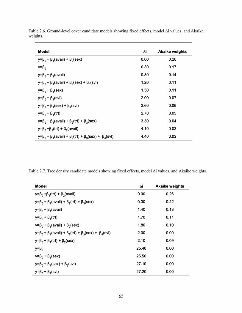
65
0.024.40y=β0 + β1(avail) + β2(trt) + β3(sex) + β4(svl)
0.034.10y=β0 +β1(trt) + β2(avail)
0.043.30y=β0 + β1(avail) + β2(trt) + β3(sex)
0.052.70y=β0 + β1(trt)
0.062.60y=β0 + β1(sex) + β2(svl)
0.072.00y=β0 + β1(svl)
0.111.30y=β0 + β1(sex)
0.111.20y=β0 + β1(avail) + β2(sex) + β3(svl)
0.140.80y=β0 + β1(avail)
0.170.30y=β0
0.200.00y=β0 + β1(avail) + β2(sex)
Akaike weights∆iModel
0.0027.20y=β0 + β1(svl)
0.0027.10y=β0 + β1(sex) + β2(svl)
0.0025.50y=β0 + β1(sex)
0.0025.40y=β0
0.092.10y=β0 + β1(trt) + β2(sex)
0.092.00y=β0 + β1(avail) + β2(trt) + β3(sex) + β4(svl)
0.101.80y=β0 + β1(avail) + β2(sex)
0.111.70y=β0 + β1(trt)
0.131.40y=β0 + β1(avail)
0.220.30y=β0 + β1(avail) + β2(trt) + β3(sex)
0.260.00y=β0 +β1(trt) + β2(avail)
Akaike weights∆iModel
Table 2.6. Ground-level cover candidate models showing fixed effects, model ∆i values, and Akaike weights. Table 2.7. Tree density candidate models showing fixed effects, model ∆i values, and Akaike weights.

66
Figure 2.1. Diagram of a LEAP array showing the arrangement of the four forest management treatments [control (CON), partial cut (PAR), clearcut with coarse woody debris (CWD) retained (RET), and clearcut with CWD removed (REM)]. The four edge types (CON/RET, PAR/RET, PAR/REM, CON/REM) and 12 release points (3 per edge) are labeled. Each treatment is approximately 4.1 ha and each edge is approximately 178 m from the wetland to the outer boundary. Figure 2.2. Diagram of microhabitat availability transects in one quadrant. Each transect was 90 m, with data recorded at 10 points at 10-m intervals. A total of 50 points were taken in each quadrant at each site.

67
0%
20%
40%
60%
80%
100%
5 m 30 m 60 m 90 m
Distance from release point
Perc
enta
ge o
f fro
gs in
fo
rest
v. c
lear
cut
Forest Clearcut
n=14n=28n=38n=44
0%
20%
40%
60%
80%
100%
5 m 30 m 60 m 90 m
Distance from release point
Perc
enta
ge o
f fro
gs in
fo
rest
v. c
lear
cut
Forest Clearcut
n=14n=28n=38n=44
0%
20%
40%
60%
80%
100%
2 m Endpoint
Distance from release point
Perc
enta
ge o
f sal
aman
ders
in
fore
st v
. cle
arcu
t
Forest Clearcut
n=44 n=33
0%
20%
40%
60%
80%
100%
2 m Endpoint
Distance from release point
Perc
enta
ge o
f sal
aman
ders
in
fore
st v
. cle
arcu
t
Forest Clearcut
n=44 n=33
Figure 2.3. Percentage of R. sphenocephala in clearcut v. forest at selected distances (5 m, 30 m, 60 m, and 90 m) from the release point on forest/clearcut edges. Figure 2.4. Percentage of A. opacum in clearcut v. forest at 2 m and endpoint from the release point on forest/clearcut edges.

68
0%
20%
40%
60%
80%
100%
5 m Endpoint
Distance from release point
Perc
enta
ge o
f toa
ds in
fo
rest
v. c
lear
cut
Forest Clearcut
n=34 n=29
0%
20%
40%
60%
80%
100%
5 m Endpoint
Distance from release point
Perc
enta
ge o
f toa
ds in
fo
rest
v. c
lear
cut
Forest Clearcut
n=34 n=29
Figure 2.5. Percentage of B. terrestris in clearcut v. forest at 5 m and endpoint from the release point on forest/clearcut edges.

69
A. B. Figure 2.6. Movement paths of R. sphenocephala at (A) site 1000 and (B) site 37. Paths are color-coded by the date the frogs were released. The black outline represents the treatment and wetland boundaries.

70
A. B. Figure 2.7 Movement paths of B. terrestris at (A) site 37 and (B) site 119. Paths are color-coded by the date the toads were released. The black outline represents the treatment and wetland boundaries.

71
A.
B. Figure 2.8. Movement paths of A. opacum at (A) site 119 and (B) site 37. Paths are color-coded by the date the salamanders were released. The black outline represents the treatment and wetland boundaries.

72
Figure 2.8C. A close-up of the A. opacum movement paths on the control/CC-removed edge at site 37.

73
10.5
86.0
46.0
0
20
40
60
80
100
R. sphenocephala A. opacum B. terrestris
Mea
n Pa
th L
engt
h (m
)
324.3
3.1 3.51.9
350.7
44.1
04080
120160200240280320360
R. sphenocephala A. opacum B. terrestris
Path
Len
gth
(m)
Minimum path length Maximum path length
Figure 2.9. Mean path length for each species. Values shown are least-squares means ± 1 standard error. Figure 2.10. Minimum and maximum path lengths for each species.

74
6.05.5
3.4
0
1
2
3
4
5
6
7
R. sphenocephala A. opacum B. terrestris
Mea
n #
Turn
s/10
m
0.61
0.69
0.78
0
0.1
0.2
0.3
0.4
0.5
0.6
0.7
0.8
0.9
R. sphenocephala A. opacum B. terrestris
Mea
n Pa
th L
inea
rity
Figure 2.11. Mean number of turns per 10 m for each species. Values shown are least-squares means ± 1 standard error. Figure 2.12. Mean path linearity for each species. Values shown are least-squares means ± 1 standard error. A linearity value of 1 represents a path that is completely straight.

75
0
20
40
60
80
100
120
R. sphenocephala A. opacum B. terrestris
Mea
n Pa
th L
engt
h (m
)Forest Clearcut
0123456789
R. sphenocephala A. opacum B. terrestris
Mea
n #
of T
urns
/10m
Forest Clearcut
Figure 2.13. Mean path length in forests v. clearcuts for each species. Values shown are least-squares means ± 1 standard error. Figure 2.14. Mean number of turns per 10 m in forests v. clearcuts for each species. Values shown are least-squares means ± 1 standard error.

76
0.00.10.20.30.40.50.60.70.80.9
R. sphenocephala A. opacum B. terrestris
Mea
n Pa
th L
inea
rity
Forest Clearcut
0102030405060708090
37 1000 37 1000 37 1000 37 1000
CON PAR RET REM
Treatment Type and Site
Mea
n co
mpo
site
inde
x of
gr
ound
-leve
l ope
nnes
s
Available ground-level openness Frog-use of ground-level openness
Figure 2.15. Mean path linearity in forests v. clearcuts for each species. Values shown are least-squares means ± 1 standard error. A linearity value of 1 represents a path that is completely straight. Figure 2.16. Mean values for ground-level openness availability v. ground-level openness use by R. sphenocephala by treatment type (control, partial, CC-retained, CC-removed) and site (37 and 1000).

77
0
1
2
3
4
5
6
37 1000 37 1000 37 1000 37 1000
CON PAR RET REM
Treatment Type and Site
Mea
n co
mpo
site
inde
x of
tr
ee d
ensi
ty
Available tree density Frog-use of tree density
0
10
20
30
40
50
60
37 1000 37 1000 37 1000 37 1000
CON PAR RET REM
Treatment Type and Site
Mea
n co
mpo
site
inde
x of
gr
ound
-leve
l cov
er
Available ground-level cover Frog-use of ground-level cover Figure 2.17. Mean values for ground-level cover availability v. ground-level cover use by R. sphenocephala by treatment type (control, partial, CC-retained, CC-removed) and site (37 and 1000). Figure 2.18. Mean values for tree density availability v. tree density use by R. sphenocephala by treatment type (control, partial, CC-retained, CC-removed) and site (37 and 1000).

1Graeter, G. J. To be submitted to Herpetological Review. 78
CHAPTER 3
THE USE OF FLUORESCENT POWDERED PIGMENTS AS AN EFFECTIVE TECHNIQUE FOR
TRACKING AMPHIBIANS1

79
INTRODUCTION
Researchers often use thread-trailing devices or radio-telemetry to study amphibian movement
and terrestrial habitat use (Sinsch 1988, Madison and Farrand 1998, Schwarzkopf and Alford 2002,
Watson et al. 2003). Fluorescent powdered pigments, used predominately for tracking small mammals,
reptiles, and insects (Johansson 1959, Lemen and Freeman 1985, Fellers and Drost 1989, Blankenship et
al. 1990, Dodd 1992, McCay 2000, Sujii et al. 2000), have recently been used successfully to track the
terrestrial movements of amphibians (Eggert 2002, Birchfield and Deters 2005). The small size and
sensitive skin of amphibians can make tracking their movements problematic, if not impossible, with
some methods. Fluorescent powder has several major advantages as a tracking method, including being
relatively inexpensive and harmless to amphibians (Rittenhouse et al. in review) and being suitable for
use on juveniles and small species. Lastly, powder tracking is particularly useful for obtaining detailed
information about an amphibian’s movement, behavior, and microhabitat use over a short time period.
Powder tracking is beginning to be recognized as an underutilized amphibian tracking method
that has great potential and may actually be the preferred method under certain circumstances
(Rittenhouse et al. in review). However, the effectiveness and limitations of this method with multiple
amphibian species under varying field conditions have not yet been explored. I present data from an
experimental field study of three species, marbled salamander (Ambystoma opacum), southern toad (Bufo
terrestris), and southern leopard frog (Rana sphenocephala) to demonstrate the potential success and
specific limitations of powder tracking as a technique for amphibians. Because little is known about the
relative distances different species can be tracked with powder, my data on powder path distances for
multiple species provides a reference that will help determine if powder tracking is the right technique for
certain species and research questions. My results also shed light on the effects of precipitation on path
length and the effectiveness of different powder colors. Lastly, I provide general recommendations
regarding the appropriate circumstances for using this technique with amphibians and how to maximize
its effectiveness.

80
MATERIALS AND METHODS
I released 44 adult A. opacum (February-March 2005), 36 adult B. terrestris (March-May 2005),
and 48 adult R. sphenocephala (May-August 2004) on forest/clearcut edges on the Savannah River Site
(SRS) in the Coastal Plain of South Carolina. The clearcuts were created in spring of 2004 as part of the
LEAP (Land-use Effects on Amphibian Populations) study. Methods used in this experiment and the
LEAP study are discussed in more detail elsewhere (see Chapter 2).
Prior to release, I applied fluorescent powder ($12/lb, Radiant Color Series T1, Richmond, CA;
now DayGlo Color Corporation, Cleveland, OH) to each individual by dipping the lower 2/3 of its body
into powder, taking care to prevent powder from coming in contact with the animal’s eyes or mouth.
Handling time was kept to less than 30 seconds. Approximately 24 hours after I released the individuals,
I tracked the path of each using a Portable Rechargeable UV Lamp (UVL-26P, Fisher Scientific
International) until I either located the animal or could not find any more powder. I used a Global
Positioning System (GPS) Trimble Pro-XR backpack unit to record each path from start to end. Then I
downloaded the GPS data and imported it into a Geographic Information System (GIS) to determine the
length of each powder path.
I used ArcView 3.3 (Environmental Systems Research Institute, Redlands, Calif.) and the Animal
Movement extension (Hooge and Eichenlaub 1997) to calculate powder path lengths for each species. To
assess how path length varied among the four powder colors, I tested the effects of powder color and
species on path length using a two-way ANOVA (Proc GLM, SAS Institute 2000). I used Tukey-
Kramer’s test to determine which colors differed from each other. I used the Type III sum of squares
because I had unequal sample sizes. Lastly, I assessed the effect of precipitation on powder path length
by examining changes in mean and maximum path length for each species with different amounts of post-
release precipitation. For this analysis, I classified rainfall based on three different precipitation classes: 0
mm, light (< 10 mm), and heavy (> 10 mm).

81
RESULTS
Path length differed significantly among species in the two-way ANOVA (Fspecies 2,120=17.52,
p<0.0001). The mean path length was shortest for A. opacum and longest for R. sphenocephala (Figure
3.1). The minimum distance an individual traveled was similar among the three species (1.9 – 3.5 m;
Figure 3.1). The maximum distance traveled by B. terrestris and R. sphenocephala was similar, but A.
opacum moved a shorter maximum distance (Figure 3.1). Similar data collected by LEAP collaborators
provide insight into the variation in efficacy of this technique among species, regions, and varying
climatic conditions (Figure 3.1). At a site in central Missouri, adult ringed salamanders (A. annulatum)
were tracked farther (3 hrs post-release; n=60) on average than the A. opacum in my study, but far shorter
distances than both B. terrestris and R. sphenocephala (Chris Conner pers. comm. 2005, Figure 3.1). In
east-central Maine, tracking (4 hrs post-release; n=10) the movement of adult wood frogs (R. sylvatica)
using fluorescent powder yielded fairly short paths (Sean Blomquist pers. comm. 2005, Figure 3.1).
Path length also varied among powder colors (Fpowder color 3,120=2.63, p=0.0536). Chartreuse paths
were the longest, pink the shortest, and green and orange were intermediate in path length (Figure 3.2).
Chartreuse and pink path lengths differed significantly from each other (p=0.0596) based on a Tukey-
Kramer test. Path length did not appear to differ among powder colors for A. opacum; however,
chartreuse path lengths were still longest for both B. terrestris and R. sphenocephala (Figure 3.3).
The amount of post-release rainfall affected powder path length. Because there was no post-
release precipitation during the B. terrestris powder tracking season, I could not look at the effects of
rainfall on path length for this species. Light amounts of precipitation (< 10 mm) did not seem to make
detection of powder more difficult (Figure 3.4a and 3.4b). However, heavy rainfall (> 10 mm) slightly
decreased the mean path length for R. sphenocephala. Most importantly, the maximum path length for R.
sphenocephala was greatly reduced after heavy rains (Figure 3.4a). Shorter paths, such as those created
by A. opacum, are apparently not negatively affected by light rainfall (Figure 3.4a)

82
DISCUSSION
Fluorescent powder tracking can be used successfully with a broad range of amphibian taxa, but
the effectiveness of the technique depends greatly on a species’ habitat use and movement range, weather
conditions, and scale of the research question. I found that amphibians can be tracked long distances (>
350 m) within a 24-hr time period under ideal conditions. The ability to detect fluorescent powder varies,
however, by powder color, especially when paths are long; when the flecks of powder become infrequent
along the powder path, some colors (e.g., chartreuse) appear brighter and are more easily detected. I also
found that fluorescent powder trails made by amphibians persisted under light rainfall, but were shortened
considerably by heavier rainfall.
The comparison of mean path lengths of A. opacum and A. annulatum confirms that this
technique has the potential to be equally successful with two closely related species in different
geographic regions (C. Conner pers. comm. 2005). However, differing environmental conditions and the
specific natural history of a species can make this technique less successful. For example, R. sylvatica
were more difficult to track with fluorescent powder than R. sphenocephala because of the wet ground
conditions at the research site in Maine (S. Blomquist pers. comm. 2005).
Some powder colors are difficult to distinguish under UV light (Stark and Fox 2000, Birchfield
and Deters 2005). I found that the pink and orange powder looked similar, as did chartreuse and green.
However, this problem could often be remedied by looking closely at the powder under a white light;
when the speck of powder was large enough, the colors could be differentiated through close
examination. Likewise, some colors are simply more difficult to detect (Stark and Fox 2000, Birchfield
and Deters 2005). This study is the first to quantify a difference in amphibian path length among powder
colors. The mean values for the path lengths of the four powder colors were as expected based on my
experience in the field; when there were small amounts of powder, chartreuse and green paths were
easiest to detect, followed by orange. Conversely, pink was the most difficult color to detect because it
was the least bright under the UV light.

83
The effect of powder color on path length was only detectable for the relatively long paths I
obtained with B. terrestris and R. sphenocephala; as path length increased, certain colors became
increasingly more difficult to detect than others. With relatively short path lengths or slow-moving
animals (e.g., A. opacum), the powder trails were heavy and color had little effect on detectability, as
found in previous studies (Birchfield and Deters 2005). Thus, although observer detection varies by
color, this probably is not a problem unless animals travel long distances.
Just as powder works better for tracking some lizard species than others because of their scale
type (Dodd 1992, Stark and Fox 2000), differing skin types in amphibians presumably affect how well the
powder clings to the skin, and thus, the efficacy of this technique with a particular species. For example,
powder stayed on B. terrestris better than A. opacum, presumably because B. terrestris has more surface
area and uneven skin that powder clings to more readily. Thus, I found that certain techniques seemed to
improve application and retention of the powder. Like many salamanders, A. opacum squirmed while
being handled, causing the powder to wipe off; thus, I suggest minimizing handling time and keeping the
powder in a small plastic container to ease application. Rana sphenocephala can also be difficult to
handle so I recommend holding the frog by its front legs with its snout in the palm of your hand while
applying powder. Lastly, the powder clung best to B. terrestris if loose soil was brushed off and the
animal’s skin was slightly moist.
The majority of the powder had usually brushed off the amphibians within 1-2 days and only
small remnants of powder were still visible on their skin. Of the B. terrestris and A. opacum I examined
in the days following powder application, most had very little powder clinging to them. I only saw R.
sphenocephala on one occasion during the post-application period, so I do not know for certain how
much powder was retained by this species. However, considering how far the R. sphenocephala moved
and that their skin has a smooth texture, the powder probably had a similar retention time to the other two
species. In a laboratory setting, where there was less opportunity to brush the powder off on natural
objects (Rittenhouse et al. in review), amphibians lost powder at a rate comparable to what I observed.

84
Others have suggested that precipitation tends to reduce the visibility of the powder trail and even
obliterate it entirely (Lemen and Freeman 1985, Blankenship et al. 1990), but to my knowledge no one
has tested how different amounts of rainfall affect the mean and maximum lengths of amphibian paths. I
found that light rainfall did not affect the maximum path length of R. sphenocephala, but that heavy
rainfall greatly truncated the maximum path length; thus, I demonstrated that fluorescent powder tracking
can be successful even with some precipitation.
Fluorescent powder, while non-toxic, is fairly persistent in the landscape (Halfpenny 1992),
particularly if there is little moisture or precipitation. Thus, in a small area, a heavy rainfall will be
necessary before powder of the same color can be used again (Stark and Fox 2000). Sometimes, powder
can remain for weeks, even after a rain, especially where powder is thickly deposited. However, the
powder is persistent in that specks of powder were found scattered throughout the study area, but the path
itself was not discernable for more than a few meters. Wind can also affect the persistence and location
of the powder (Eggert 2002); however, I only found the wind problematic when already sparse powder
became scattered and when two or more paths of similar color crossed one another.
Recommendations
Before deciding to use fluorescent powder for tracking amphibians, several points should be
considered. First, because powder paths usually persist only 1-2 days from application, this technique is
most effective in answering questions about fine-scale movement and microhabitat use. For example, I
could discern whether an individual had rested on woody debris or moved under it, the type of vegetation
they had traveled through or avoided, and what type of cover they selected. If one were interested in
answering long-term questions, powder could be reapplied, but this has the obvious disadvantage of
influencing the animal’s behavior. The success of this technique can also be influenced by the natural
history of a species. For example, if the species periodically spends time in an aquatic or moist
environment or burrows underground, it will be more difficult to track with powder (S. Blomquist pers.
comm. 2005, Eggert 2002). In addition, the distance a species moves can affect the ease of detecting the

85
powder and differentiating between multiple paths. For instance, if a species’ movements are
concentrated within a small area, it can be difficult to follow the path when powder trails cross (Stark and
Fox 2000).
Weather conditions, as well as site and regional differences, can also affect the suitability of
fluorescent powder as a tracking technique for amphibians. For example, in areas where field conditions
are typically moist, as they are at the LEAP study area in Maine (S. Blomquist pers. comm. 2005),
powder tracking may not be as informative or useful as it is in drier regions. Similarly, some studies have
suggested that vegetation type can affect how well the technique works (Mullican 1988, Eggert 2002),
which obviously varies among research locations. Finally, in situations where paths are unlikely to
overlap (e.g., individuals are being tracked in separate locations) and only one powder color is needed,
chartreuse may be the optimum color to use.
My research has demonstrated that fluorescent powder tracking can be very effective at obtaining
detailed movement and habitat use data for a variety of amphibian species. For example, it can be used to
look at detailed movements, to assess whether certain habitats have been sampled, to test the effectiveness
of other research methods, and as a supplement to other amphibian research techniques. However, the
usefulness of this technique may vary by region, by the particular environmental conditions of a research
site, and by the habitat use and movement behavior of the study species.
ACKNOWLEDGEMENTS
Research and manuscript preparation were aided by the Environmental Remediation Sciences
Division of the Office of Biological and Environmental Research, U.S. Department of Energy
through Financial Assistance Award no. DE-FC09-96SR18546 to the University of Georgia Research
Foundation and by National Science Foundation Grant #DBI-0139572. The procedures used in this study
were approved by the University of Georgia animal care and use committee (A2003-10024, "Reptile and
Amphibian Research--General Field Studies") and the South Carolina Department of Natural Resources
(collection permits: 56-2003, 07-2004). I thank D. S. Berry, S. E. DuRant, A. D. Green, M. Langley, T.

86
M. Luhring, J. P. Nestor, B. B. Rothermel, J. D. Willson, C. T. Winne, and M. S. Wright for field
assistance, C. A. Conner and S. M. Blomquist for the fluorescent powder tracking data they provided, and
C. R. Carroll, M. C. Freeman, J. W. Gibbons, and B. B. Rothermel for providing useful comments on the
manuscript.
LITERATURE CITED
Birchfield, G. L., and J. E. Deters. 2005. Movement paths of displaced northern green frogs (Rana clamitans melanota). Southeastern Naturalist 4:63-76.
Blankenship, E. L., T. W. Bryan, and S. P. Jacobsen. 1990. A method for tracking tortoises using fluorescent powder. Herpetological Review 21:88-89.
Dodd, C. K. 1992. Fluorescent powder is only partially successful in tracking movements of the six-lined racerunner (Cnemidophorus sexlineatus). Florida Field Naturalist 20:8-14.
Eggert, C. 2002. Use of fluorescent pigments and implantable transmitters to track a fossorial toad (Pelobates fuscus). Herpetological Journal 12:69-74.
Fellers, G. M., and C. A. Drost. 1989. Fluorescent powder: a method for tracking reptiles. Herpetological Review 20:91-92.
Halfpenny, J. C. 1992. Environmental impacts of powdertracking using fluorescent pigments. Journal of Mammalogy 73:680-682.
Hooge, P. N., and B. Eichenlaub. 1997. Animal Movement extension to ArcView; SA ver. 2.04 beta. in. Alaska Science Center - Biological Science Office, U.S. Geological Survey, Anchorage, AK, USA.
Johansson, T. S. K. 1959. Tracking honey bees in cotton fields with fluorescent pigments. Journal of Economic Entomology 52:572-577.
Lemen, C. A., and P. W. Freeman. 1985. Tracking mammals with fluorescent pigments: a new technique. Journal of Mammalogy 66:134-136.
Madison, D. M., and L. Farrand. 1998. Habitat use during breeding and emigration in radio-implanted tiger salamanders, Ambystoma tigrinum. Copeia 2:402-410.
McCay, T. S. 2000. Use of woody debris by cotton mice (Peromyscus gossypinus) in a southeastern pine forest. Journal of Mammalogy 81:527-535.
Mullican, T. R. 1988. Radio telemetry and fluorescent pigments - a comparison of techniques. Journal of Wildlife Management 52:627-631.
Rittenhouse, T. A. G., T. A. Altnether, and R. D. Semlitsch. in review. Florescent powder pigments as a harmless tracking method for ambystomatids and ranids. Herpetological Review.

87
SAS Institute, I. 2000. SAS Proprietary Software Release 9.1, Cary, North Carolina.
Schwarzkopf, L., and R. A. Alford. 2002. Nomadic movement in tropical toads. Oikos 96:492-506.
Sinsch, U. 1988. Seasonal changes in the migratory behavior of the toad Bufo bufo - direction and magnitude of movements. Oecologia 76:390-398.
Stark, R. C., and S. F. Fox. 2000. Use of fluorescent powder to track horned lizards. Herpetological Review 31:230-231.
Sujii, E. R., M. A. Garcia, and E. M. G. Fontes. 2000. Movements of migration and dispersion of adult spittlebugs. Pesquisa Agropecuaria Brasileira 35:471-480.
Watson, J. W., K. R. McAllister, and D. J. Pierce. 2003. Home ranges, movements, and habitat selection of Oregon spotted frogs (Rana pretiosa). Journal of Herpetology 37:292-300.

88
133.8
10.4
85.444.1
12.7 36.93.5 2.63.1 2.41.9
324.3 350.7
27.3 44.1
050
100150200250300350400
B. terre
stris
R. sph
enoce
phala
R. sylv
atica
A. opa
cum
A. ann
ulatum
Path
Len
gth
(m)
Mean Minimum Maximum
(n=36) (n=44) (n=10) (n=44) (n=60)
133.8
10.4
85.444.1
12.7 36.93.5 2.63.1 2.41.9
324.3 350.7
27.3 44.1
050
100150200250300350400
B. terre
stris
R. sph
enoce
phala
R. sylv
atica
A. opa
cum
A. ann
ulatum
Path
Len
gth
(m)
Mean Minimum Maximum
(n=36) (n=44) (n=10) (n=44) (n=60)
Figure 3.1. Mean, minimum, maximum path lengths of A. opacum, B. terrestris, and R. sphenocephala in S.C. (this study), A. annulatum in M.O. (C. Conner pers. comm. 2005), and R. sylvatica in M.E. (S. Blomquist pers. comm. 2005). Mean path length values have ± 1 standard error.

89
0
20
40
60
80
100
120
140
A. opacum B. terrestris R. sphenocephala
Mea
n P
ath
Leng
th (m
)
pink orange green chartreuse
(n=44) (n=36) (n=44)
0
20
40
60
80
100
120
140
A. opacum B. terrestris R. sphenocephala
Mea
n P
ath
Leng
th (m
)
pink orange green chartreuse
(n=44) (n=36) (n=44)
0
10
20
30
40
50
60
70
80
pink orange green chartreuse
Powder Color
Mea
n Pa
th L
engt
h (m
)
(n=28) (n=35) (n=27) (n=34)
0
10
20
30
40
50
60
70
80
pink orange green chartreuse
Powder Color
Mea
n Pa
th L
engt
h (m
)
(n=28) (n=35) (n=27) (n=34)
Figure 3.2. Mean path length for the four fluorescent powder colors. Values are least squares means ± 1 standard error from the two-way ANOVA with species and powder color as effects. Figure 3.3. Mean path length for powder color, specific to species. Values are least squares means ±1 standard error.

90
0
100
200
300
400
0 mm <10 mm >10 mm
Amount of Precipitation
Path
Len
gth
(m)
Mean Path Length Maximum Path Length
A. Rana sphenocephala
0
100
200
300
400
0 mm <10 mm >10 mm
Amount of Precipitation
Path
Len
gth
(m)
Mean Path Length Maximum Path Length
A. Rana sphenocephala
0
10
2030
40
50
0 mm <10 mm
Amount of Precipitation
Path
Len
gth
(m)
Mean Path Length Maximum Path Length
B. Ambystoma opacum
0
10
2030
40
50
0 mm <10 mm
Amount of Precipitation
Path
Len
gth
(m)
Mean Path Length Maximum Path Length
B. Ambystoma opacum
Figure 3.4. Relationship between post-release precipitation and mean and maximum powder path length in (A) R. sphenocephala at three different precipitation levels and (B) in A. opacum at two different precipitation levels. No rainfall greater than 10 mm was recorded during the A. opacum releases, thus, that category is not included.

91
CHAPTER 4
CONCLUSION
In this study, I examined the effects of forest management on habitat selection and movement
behavior of adult amphibians and evaluated the efficacy of the fluorescent powder tracking technique for
amphibians. Using the experimental releases on forest/clearcut edges, I demonstrated that marbled
salamanders (A. opacum) selected habitat at random, southern toads (B. terrestris) preferred clearcuts, and
southern leopard frogs (R. sphenocephala) initially selected clearcuts, but may have ultimately preferred
forests. These results indicate that both B. terrestris and R. sphenocephala are capable of differentiating
between habitat types and do not necessarily avoid recently cleared areas. Ambystoma opacum may not
be able to differentiate between habitats or require more time (> 24 hrs) to select non-breeding habitat.
I also found that the manner in which amphibians move can vary greatly among species and
habitat types. Whereas leopard frogs exhibited long-distance, directional movement with few turns,
southern toads exhibited more searching and wandering behavior. Marbled salamanders seemed to be
focused primarily on locating cover. All three species made more turns in clearcuts than forests, and B.
terrestris and R. sphenocephala moved farther in forests. None of the environmental cues or individual
characteristics I measured appeared to influence habitat selection by R. sphenocephala or B. terrestris.
Ambystoma opacum were more likely to enter clearcuts if soil moisture content was higher. Rana
sphenocephala generally used microhabitat relative to what was available, but avoided microhabitat, such
as the large amounts of debris in the clearcuts with CWD retained, that might obstruct movement.
Amphibian habitat selection and movement behavior and the differences among species are important
because they affect individual fitness and even population dynamics.

92
My examination of the efficacy of fluorescent powdered pigments for tracking amphibian
movement demonstrated some important differences. First, the efficacy of this technique varied among
species, regions, and varying climatic conditions. The technique tended to be more effective in pine
habitat in South Carolina (this study) and mixed hardwood habitat in Missouri (data from C. Conner
2005) than in the mixed hardwood habitat in Maine (data from S. Blomquist 2005) where the ground
moisture was high. I found that while the powder colors gave comparable path lengths when animals
moved short distances in my study, certain powder colors (i.e., chartreuse) were easier to detect when
paths were long and the powder began to wear off. Lastly, I demonstrated that heavy rainfall truncated
paths, but light rainfall had no negative effect on path length.
This study highlights the importance of species-specific information when it comes to assessing
the effects of habitat disturbance on amphibians; information of this type is greatly needed for modeling
amphibian habitat use and movements in order to make more informed conservation decisions. I also
demonstrated that fluorescent powder tracking can be used successfully with a broad range of amphibian
taxa, but the effectiveness of the technique depends greatly on a species’ habitat use and movement range,
and the weather conditions and scale of the research question. Knowledge of individual species’
responses to forest alteration enables land managers and conservationists to make relevant species-
specific forest management decisions.