habit formation and precautionary saving: evidence from the korean

JOURNAL OF ECONOMIC DEVELOPMENT 1 Volume 29, Number 2, December 2004

HABIT FORMATION AND PRECAUTIONARY SAVING: EVIDENCE

FROM THE KOREAN HOUSEHOLD PANEL STUDIES

WOOHEON RHEE*

Kyunghee University

We examined the evidence of precautionary saving and Constantinides (1990) type habit formation model by using the Korean Household Panel Studies, which has six years of time series observations and thousands of cross section observations. Employing the dynamic panel data estimation method, we found that the estimates of parameters corresponding to the degree of habit formation and precautionary saving are statistically insignificant for food consumption, but statistically significant or at least marginally significant for nondurables and services consumption.

Keywords: Habit Formation, Precautionary Saving, Korean Household Panel Studies, Dynamic Panel Data Estimation

JEL classification: E200, C520

1. INTRODUCTION Recently, we have observed growing interest in habit formation in consumption as a

way of resolving the unsatisfactory performance of the simple permanent income-life cycle hypothesis, and some well-known anomalies in financial markets. For example, Constantinides (1990), Abel (1990), Campbell and Cochrane (1999) show that some well-known anomalies such as the risk premium puzzle and poor performance of the Consumption CAPM documented in finance literature can be reasonably well resolved once we consider habit formation in consumption. However, despite the increasing

* The author is grateful to Seungchan Ahn, Soyoung Kim, Hyungsik Roger Moon, seminar participants at

the Fall Camp of the Korean Econometrics Association November 2001, an anonymous referee for helpful comments, and especially to Karen Dynan for her insights and comments. The author also wishes to acknowledge Dr. Young Bae Moon’s assistance in constructing SAS codes. Financial support from Sungkok Research Foundation and Kyunghee University is greatly appreciated. Any remaining errors are the responsibility of the author.

WOOHEON RHEE 2

interest in habit formation in theory, and some empirical support for it from aggregate data, there are not many studies on habit formation that examine micro level data. Among the few, Dynan (2000) examined the PSID and found little evidence of it. It is therefore necessary to examine other sources of micro level data and to see if there is any evidence of habit formation. This paper aims to fill the gap by examining the Korean Household Panel Studies (henceforth KHPS).

At the same time, we will also examine if we can find some evidence of precautionary saving using the KHPS data. To our limited knowledge, there is little empirical research, except Mckenzie (2001), that examines and evaluates both habit formation and precautionary saving in a single framework. This may be due mainly to the lack of data. That is, it is very hard to find an exogenous source of uncertainty about future income. However, the KHPS allows us to examine both habit formation and precautionary saving in a single framework. We can do this by employing two variables; the number of earners in a family, and the job security evaluated by the head of household as a proxy for the uncertainty faced by a household. We expect that as the number of earners in a family increases, there is less risk of catastrophic drop in income, and accordingly, less incentive for precautionary saving. We also expect that as the uncertainty faced by a household decreases, there is less incentive for precautionary saving. We will examine these implications in this study.

The KHPS had been collected by the Daewoo Economic Research Institute for the period between 1993 and 1998, and was discontinued in 1999 when the Daewoo Conglomerate went bankrupt during the aftermath of the Asian currency crisis. The KHPS is composed of household and individual files. The household files surveyed a couple of thousand households each year and the individual files surveyed individuals in the household files. The KHPS reports several interesting questions including the job security of individuals as well as basic numbers such as consumption expenditures on various items, incomes from various sources, assets and liabilities in various forms. This is the greatest advantage of the KHPS over the most widely studied data, the PSID, which reports expenditures only on food.

We will examine the evidence of habit formation by regressing the current consumption growth rate on the one-period lagged consumption growth rate, and seeing if the estimate is positive. In order to estimate the model, we will employ the dynamic panel data estimation method developed by Arellano and Bond (1991, 1998), and Blundell and Bond (1998). This method computes GMM estimators, and can be well applied to panel data with small time series observations and relatively large cross section observations, which is exactly the case of the KHPS.

In section II, we present a simple model of habit formation and precautionary saving, which draws on Hayashi (1985) and Dynan (2000). In section III, we describe the KHPS data in detail and explain our estimation strategy. We present estimation results in section IV, and some concluding remarks in section V.

HABIT FORMATION AND PRECAUTIONARY SAVING 3

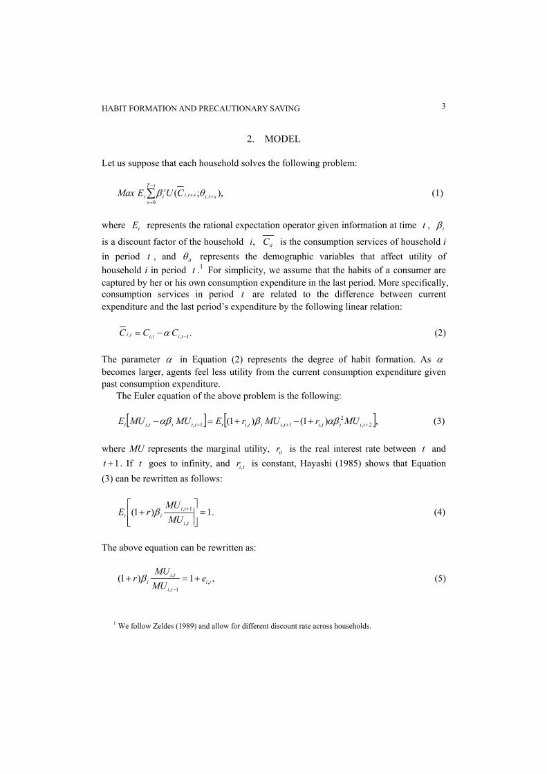
2. MODEL

Let us suppose that each household solves the following problem:

),;( ,,0

stisti

tT

s

sit CUEMax ++

−

=∑ θβ (1)

where represents the rational expectation operator given information at time ,

is a discount factor of the household tE t iβ

,i itC is the consumption services of household i in period , and represents the demographic variables that affect utility of household i in period .

t itθt 1 For simplicity, we assume that the habits of a consumer are

captured by her or his own consumption expenditure in the last period. More specifically, consumption services in period are related to the difference between current expenditure and the last period’s expenditure by the following linear relation:

t

.1,,, −−= tititi CCC α (2)

The parameter α in Equation (2) represents the degree of habit formation. As α becomes larger, agents feel less utility from the current consumption expenditure given past consumption expenditure.

The Euler equation of the above problem is the following:

[ ] [ ],)1()1( 2,2

,1,,1,, +++ +−+=− tiititiitittiitit MUrMUrEMUMUE αββαβ (3) where MU represents the marginal utility, is the real interest rate between and

. If goes to infinity, and is constant, Hayashi (1985) shows that Equation (3) can be rewritten as follows:

itr t1+t t tir ,

.1)1(,

1, =

+ +

ti

tiit MU

MUrE β (4)

The above equation can be rewritten as:

,1)1( ,1,

,ti

ti

tii e

MUMU

r +=+−

β (5)

1 We follow Zeldes (1989) and allow for different discount rate across households.

WOOHEON RHEE 4

where denotes the forecast error. tie ,

Let us assume that the utility function takes the form of commonly used constant relative risk aversion:

,1

)exp();(1,

,,,γ

θθγ

−=

−ti

tititiCCU (6)

where γ represents the degree of relative risk aversion. If we combine Equations (5) and (6), we have:

,1)exp()1( ,1,

,, ti

ti

titii e

CCr +=

∆+

−

−

γ

θβ (7)

where (and equations below) represents the first difference of the variable x∆ x . If we take natural logarithms on both sides of Equation (7), we have:

( ) ( ).)1ln(ln)1ln(1ln ,,1,, titiititi erCC +−∆+++=−∆ − θβγ

α (8)

Following Muellbauer (1988), Dynan (2000) approximates the left hand side of

Equation (8) as:

( ) .lnlnln 1,,1,, −− ∆−∆≈−∆ titititi CCCC αα (9)

Combining Equations (8) and (9), we have:

( ) ).1ln(1ln1ln)1ln(1ln ,1,,, tititiiti eCrC +−∆+∆+++≈∆ − γαθ

γβ

γ (10)

If we take the second order approximation of the last term in Equation (10), we have:

( ) ,2

ln1ln)1ln(1ln ,

2,

1,,, titi

titiiti uCrC ++∆+∆+++≈∆ − γσ

αθγ

βγ

(11)

where ( )γσ

γ 21ln1 2

,2,

,,titi

titi

eeu

−++−= with mean zero.

It has been noticed that the consumption data has some measurement error, and it


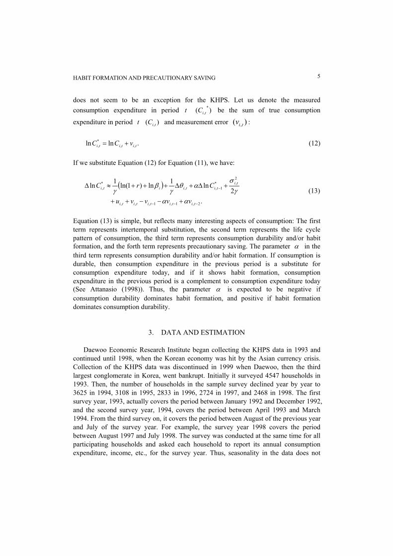
does not seem to be an exception for the KHPS. Let us denote the measured consumption expenditure in period t ) be the sum of true consumption

expenditure in period and measurement error :

( *,tiC

t )( ,tiC )( ,tiv

.lnln ,,*, tititi vCC += (12)

If we substitute Equation (12) for Equation (11), we have:

( )

.2

ln1ln)1ln(1ln

2,1,1,,,

2,*

1,,*,

−−−

−

+−−++

+∆+∆+++≈∆

tititititi

tititiiti

vvvvu

CrC

ααγ

σαθ

γβ

γ (13)

Equation (13) is simple, but reflects many interesting aspects of consumption: The first term represents intertemporal substitution, the second term represents the life cycle pattern of consumption, the third term represents consumption durability and/or habit formation, and the forth term represents precautionary saving. The parameter α in the third term represents consumption durability and/or habit formation. If consumption is durable, then consumption expenditure in the previous period is a substitute for consumption expenditure today, and if it shows habit formation, consumption expenditure in the previous period is a complement to consumption expenditure today (See Attanasio (1998)). Thus, the parameter α is expected to be negative if consumption durability dominates habit formation, and positive if habit formation dominates consumption durability.

3. DATA AND ESTIMATION Daewoo Economic Research Institute began collecting the KHPS data in 1993 and

continued until 1998, when the Korean economy was hit by the Asian currency crisis. Collection of the KHPS data was discontinued in 1999 when Daewoo, then the third largest conglomerate in Korea, went bankrupt. Initially it surveyed 4547 households in 1993. Then, the number of households in the sample survey declined year by year to 3625 in 1994, 3108 in 1995, 2833 in 1996, 2724 in 1997, and 2468 in 1998. The first survey year, 1993, actually covers the period between January 1992 and December 1992, and the second survey year, 1994, covers the period between April 1993 and March 1994. From the third survey on, it covers the period between August of the previous year and July of the survey year. For example, the survey year 1998 covers the period between August 1997 and July 1998. The survey was conducted at the same time for all participating households and asked each household to report its annual consumption expenditure, income, etc., for the survey year. Thus, seasonality in the data does not

WOOHEON RHEE 6

seem to be a serious problem. The KHPS consists of two parts; one is the household file and the other is the

individual file. The household file reports basic data for each household, and the individual file reports data for the individuals in the household. The KHPS is a valuable panel data in the sense that it reports many interesting questions and covers various ranges of consumption expenditures, incomes, assets and liabilities. For example, it reports job security evaluated by individual members of the household, and reports expenditures on various items of nondurables and services as well as durables (including automobiles). This is the greatest advantage of the KHPS over the most widely studied data, the PSID, which reports expenditures only on food.

Let us briefly describe the data that will be used in this study. The KHPS household file surveys expenditures on nondurables and services. It reports expenditures on food, rent, clothing, footwear, entertainment, heating, medical care, education, day care, restaurants, vacation, etc., We get real household consumption of nondurables and services by deflating each item by the sample period average of the corresponding consumer price index published by the National Statistics Office (NSO).

As demographic variables ( , we will consider the following variables; age, square of age, education level of the head of household, family size, number of earners, and the dependency ratio of each household. All of the variables are directly from the KHPS except the number of earners and the dependency ratio,

)itθ

2 which we constructed from the original data. We will also add several demographic dummy variables for the head of household in the regression analysis such as a dummy for sex, dummies for marital status, dummies for home ownership, and dummies for job.

The KHPS reports an interesting variable in the individual file, that is, the job security (jobsec in the regression equation) evaluated by each individual. The survey asked each individual to evaluate her or his job security on a scale of 1 to 5, with the higher rating indicating more secure jobs. Thus, job security increases as the rating of this variable increases from 1 to 5.

In estimating the model, we first chose households that existed during the whole sample period, and got 2266 households. Then, we removed all the households that had missing values in any of consumption expenditures, demographic variables, and job security evaluated by the head of household.3 Out of the 2266 households, we had 1766 households in the case of food consumption and 1093 households in the case of nondurables and services consumption. We had far fewer households for the analysis of nondurables and services consumption than food consumption because the former covers much broader ranges of consumption than the latter, and accordingly, has more chance of containing missing values. Among the items of nondurables and services,

2 The dependency ratio is constructed as the ratio of members under age 15 and over 65 to the total

number of family members. 3 Most households except very few report demographic variables.


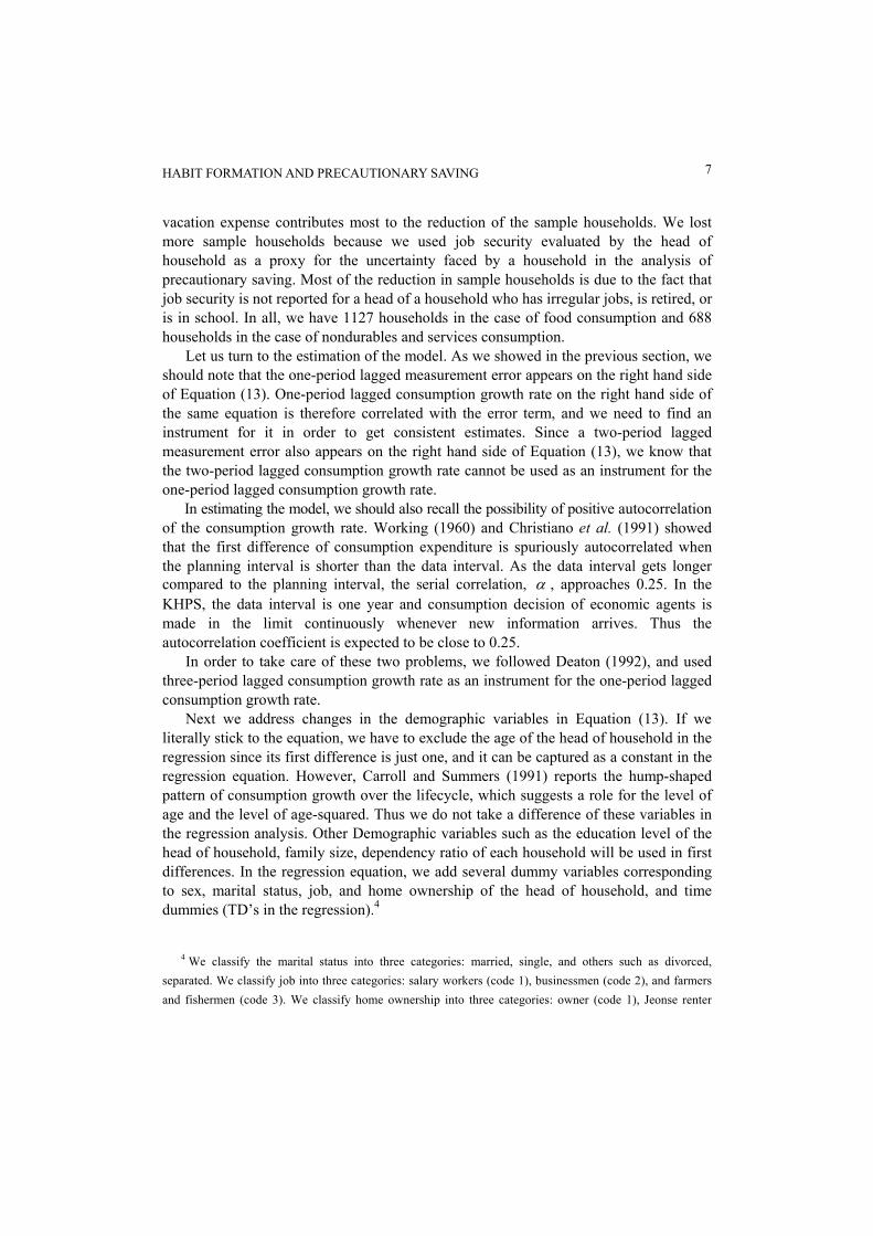
vacation expense contributes most to the reduction of the sample households. We lost more sample households because we used job security evaluated by the head of household as a proxy for the uncertainty faced by a household in the analysis of precautionary saving. Most of the reduction in sample households is due to the fact that job security is not reported for a head of a household who has irregular jobs, is retired, or is in school. In all, we have 1127 households in the case of food consumption and 688 households in the case of nondurables and services consumption.

Let us turn to the estimation of the model. As we showed in the previous section, we should note that the one-period lagged measurement error appears on the right hand side of Equation (13). One-period lagged consumption growth rate on the right hand side of the same equation is therefore correlated with the error term, and we need to find an instrument for it in order to get consistent estimates. Since a two-period lagged measurement error also appears on the right hand side of Equation (13), we know that the two-period lagged consumption growth rate cannot be used as an instrument for the one-period lagged consumption growth rate.

In estimating the model, we should also recall the possibility of positive autocorrelation of the consumption growth rate. Working (1960) and Christiano et al. (1991) showed that the first difference of consumption expenditure is spuriously autocorrelated when the planning interval is shorter than the data interval. As the data interval gets longer compared to the planning interval, the serial correlation, α , approaches 0.25. In the KHPS, the data interval is one year and consumption decision of economic agents is made in the limit continuously whenever new information arrives. Thus the autocorrelation coefficient is expected to be close to 0.25.

In order to take care of these two problems, we followed Deaton (1992), and used three-period lagged consumption growth rate as an instrument for the one-period lagged consumption growth rate.

Next we address changes in the demographic variables in Equation (13). If we literally stick to the equation, we have to exclude the age of the head of household in the regression since its first difference is just one, and it can be captured as a constant in the regression equation. However, Carroll and Summers (1991) reports the hump-shaped pattern of consumption growth over the lifecycle, which suggests a role for the level of age and the level of age-squared. Thus we do not take a difference of these variables in the regression analysis. Other Demographic variables such as the education level of the head of household, family size, dependency ratio of each household will be used in first differences. In the regression equation, we add several dummy variables corresponding to sex, marital status, job, and home ownership of the head of household, and time dummies (TD’s in the regression).4

4 We classify the marital status into three categories: married, single, and others such as divorced, separated. We classify job into three categories: salary workers (code 1), businessmen (code 2), and farmers and fishermen (code 3). We classify home ownership into three categories: owner (code 1), Jeonse renter

WOOHEON RHEE 8

In order to evaluate the significance of the precautionary saving motives, we will consider two variables; number of earners in a household (nearn) and the job security evaluated by the head of household (jobsec). Number of earners in a household is a demographic variable that is expected to be related to the precautionary saving motives. If there are more earners in a family, there would be less risk of a catastrophic drop in family income, and there would be less incentive for precautionary saving. Job security evaluated by the head of household can represent uncertainty about future income as we discussed in the above. We assume that the uncertainty faced by a household linearly declines as the score of job security (jobsec

)( ,2

tiσ

i,t) increases, and will use job security of the head of household as a proxy for the uncertainty faced by the household. One may suspect that the variable jobsec may carry the information about not only the expected second moment of income growth, but also the expected first moment of income growth. That is, a decrease in the variable is not a mean preserving increase in uncertainty, but rather embodies both a reduction in mean and an increase in variance. Certainly, we cannot rule out this possibility. However, right before it asks about the job security, the survey also asks each individual to evaluate the level of income (and/or income growth) of the job on a scale of 1 to 5, with a higher rating indicating higher income level (and/or growth) relative to the average income level (and/or growth). Thus, it seems that the variable jobsec is intended to ask about the second moment of income growth. Furthermore, even if jobsec carries information about both the expected first and second moments of income growth, it is not expected to qualitatively affect the results, since precautionary saving is captured by the second moment of expected income growth and the effect of the first moment of expected income growth on consumption growth whatsoever should be adjusted by the constant term.

The final equation to be estimated has the following form:5

,secln

tanln

,1,21,1*

1,

,1,0*,

titititi

titititi

jobnearnC

bbTDFEtconsC

εββα

θθ

+++∆+

+∆+++≈∆

−−−

(14)

where represents the household specific effect, and . Note that in the equation above, we use one-period lagged value of number of earners (nearn) and job security (jobsec). When uncertainty increases, consumers reduce consumption in the current period and accumulate wealth. This would reduce the

iFE 2,1,1,,,, −−− +−−+= titititititi vvvvu ααε

(code 2), and monthly renter (code 3). Jeonse is a Korean style rental system, where renters pay down payment of about 60 to 70% of the price of a house to the owner and rent it for two years. The Jeonse contract can be renewed every two years. After the rent is over, renters are paid back their down payments from the owner.

5 We include dummy variables corresponding to sex, marital status, job, and home ownership of the head of household in in order to save notations. ti,θ


incentive for saving next period. Thus, there would be a positive relationship between uncertainty evaluated at present and expected consumption growth rate between the present and the next period. Similar reasoning can be applied to the number of earners. We expect both and to be negative if the precautionary saving motive is important, since a higher number of earners reduces the incentive for precautionary saving and a larger rating of jobsec means more stable job security, and accordingly, less uncertainty about future income. Though not explicitly shown in Equation (14), we also use one-period lagged values of dummies for job and home ownership. These dummies can also be related to precautionary saving motives. For example, if a family owns a house, it may have less incentive for precautionary saving since the house can be used as an insurance against a sudden drop in income. Job dummies may also be related to precautionary saving motives as we will discuss in the next section.

1β 2β

Equation (14) has a lagged dependent variable on the right hand side, and it is sometimes called a dynamic panel regression. In order to estimate this equation, we employ the dynamic panel data estimation method (henceforth DPD) developed by Arellano and Bond (1991, 1998), and Blundell and Bond (1998). This estimation method suits for our purpose in several ways. First, the DPD can be well applied to a panel with few time series observations and relatively large cross section observations. This is exactly the case of the KHPS, which has six years of time series observation, and much more cross section observations. Second, DPD is an efficient estimation in the case where there is heteroskedasticity. We consider demographic variables in order to capture household specific behavior in consumption growth rates. However, there may still exist missing elements that we do not consider, and this may result in heteroskedasticity in the error terms. Third, DPD takes the second order moving average error structure in the estimation Equation (14) into account.

The DPD estimation of Arellano and Bond (1998), and Blundell and Bond (1998) produces linear GMM estimators for three cases; one step estimates, one-step and two-step estimates with heteroskedasticity consistent standard errors (See more details in Arellano and Bond (1998)). In the next section, we will report all three cases in order to check robustness of the results across estimation methods.

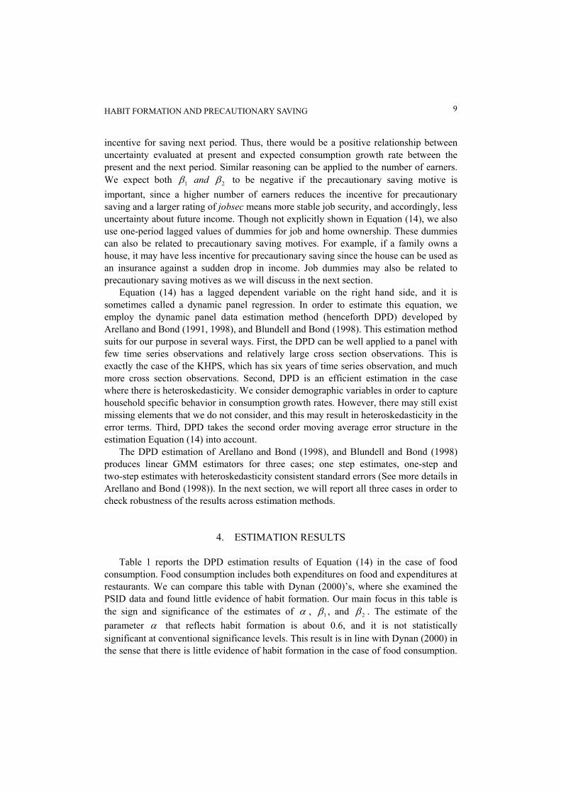
4. ESTIMATION RESULTS Table 1 reports the DPD estimation results of Equation (14) in the case of food

consumption. Food consumption includes both expenditures on food and expenditures at restaurants. We can compare this table with Dynan (2000)’s, where she examined the PSID data and found little evidence of habit formation. Our main focus in this table is the sign and significance of the estimates of α , , and . The estimate of the parameter

1β 2βα that reflects habit formation is about 0.6, and it is not statistically

significant at conventional significance levels. This result is in line with Dynan (2000) in the sense that there is little evidence of habit formation in the case of food consumption.

WOOHEON RHEE 10

The parameter estimates for the number of earners in a family and job security of the head of household, both of which are expected to capture precautionary saving motives are negative, respectively, whatever the estimation method is. Thus, the sign of these coefficients are consistent with the prediction of precautionary saving theory. However, they are not statistically significantly different from 0.

The twelve demographic variables as a whole including various dummy variables are significant at 1% significance level as the Wald test statistic shows. This is mainly due to the high significance of the job dummy variables. As we can see in the table, job dummy variables are negative and highly significant, implying that the growth rate of food consumption of salary workers and businessmen are lower than that of farmers and fishermen. Some may suspect that this may be regarded as an evidence of precautionary saving since agents’ job choice and attitudes towards risk may be correlated (See Skinner (1988) and Mckenzie (2001)). More risk averse agents will choose more secure jobs.

Table 1. DPD Estimation Results: Food (number of sample households = 1127)

,secln

ln

,1,21,1*

1,

,1,0*,

titititi

titititi

jobnearnC

bbTDEffectFixedttanconsC

εββα

θθ

+++∆+

+∆+++≈∆

−−−

A: One-Step Estimates ∆lnCi,t-1 0.56 (1.16)

∆θi,t

Family size Dependency Ratio Education Level

0.032 (0.77) 0.013 (0.08)

-0.055 (-1.28)

θi,t

Age Square of Age Male Married Single Home Owner Jeonse (2 Year Rent) Salary Workers Businessmen

0.0050 (0.46) -0.000027 (-0.24) 0.091 (0.79)

-0.068 (-0.66) 0.097 (0.56)

-0.0093 (-0.16) -0.0057 (-0.09) -0.09 (-2.02)** -0.17 (-4.02)***

Number of Earners (nearn) -0.039 (-1.15) Job security (jobsec) -0.0066 (-0.38) Time Dummy (TD) for 1998 -0.15 (-3.56)*** Wald statistic for 0,, ==∆ titi θθ 34.63 (0.001)+


B: One-Step Estimates with Heteroskedasticity-Consistent Standard Errors ∆lnCi,t-1 0.56 (1.13) ∆θi,t


0.032 (0.55) 0.013 (0.07)

-0.055 (-1.48) θi,t


0.0050 (0.50) -0.000027 (-0.26) 0.091 (0.79)

-0.068 (-0.74) 0.097 (0.65)

-0.0093 (-0.19) -0.0057 (-0.11) -0.09 (-1.82)* -0.17 (-3.51)***


C: Two-Step Estimates with Heteroskedasticity-Consistent Standard Errors ∆lnCi,t-1 0.62 (1.28) ∆θi,t


0.033 (0.58) -0.010 (-0.05) -0.062 (-1.70)*

θi,t


0.0051 (0.51) -0.000026 (-0.24) 0.093 (0.81)

-0.056 (-0.62) 0.12 (0.79)

-0.014 (-0.29) -0.0084 (-0.16) -0.10 (-2.13)** -0.18 (-3.79)***


Numbers in parentheses are t statistics. *, **, *** significant at 10%, 5%, and 1% level, respectively. + represents p-values.

WOOHEON RHEE 12

In Korea, at least before the Asian currency crisis, when traditional lifetime employment ceased to be the convention, more risk averse agents tended to be employed as salary workers rather than run her or his own business. This possibility can be confirmed by the correlation between job security and job dummy variables. In our sample, the correlation between job dummy 1 (salary workers) and job security is 0.22, and the correlation between job dummy 2 (businessmen) and job security is -0.1. Thus, salary workers tend to face more secure job than businessmen. Precautionary saving theory suggests more prudence for salary workers in the sense that they are more risk averse, and at the same time less prudence for salary workers in the sense that they have more secure jobs and less uncertainty about their future income.

With all these possibilities, the results in Table 1 do not seem to support the precautionary saving theory. Once job security is controlled by the variable jobsec, salary workers are expected to show more prudence than businessmen in the sense that they are more risk averse. However, the absolute value of the coefficient of job dummy 1 (salary workers) is smaller and less significant than that of job dummy 2 (businessmen) in all cases, which contradicts the implications of precautionary saving theory. In addition, the coefficient of the dummy variable for home owners is also insignificant, though it is negative. This is also an evidence against the precautionary saving theory.

In every case, the time dummy for 1998 has negative value and is statistically highly significant. This implies that households reduced their consumption expenditure significantly in 1998 when the Korean economy was severely hit by the Asian currency crisis. This may partly reflect the precautionary saving behavior not captured by the number of earners in a family and job security of the head of household in the regression equation. Asian currency crisis started in August 1997 when Thailand succumbed to the speculative attack and gave up defending Baht. Korea also gave in to the attack in December 1997, and asked for help from the IMF, and the Korean economy experienced an unprecedented severe downturn in the first half of 1998. This period (August 1997 - July 1998) is exactly the period covered by the 1998 survey. During this period, several commercial banks were closed, many firms went bankrupt, and many workers were removed from their previously thought to be pseudo-permanent jobs. This was the period of catastrophic disaster to at least some households in Korea.

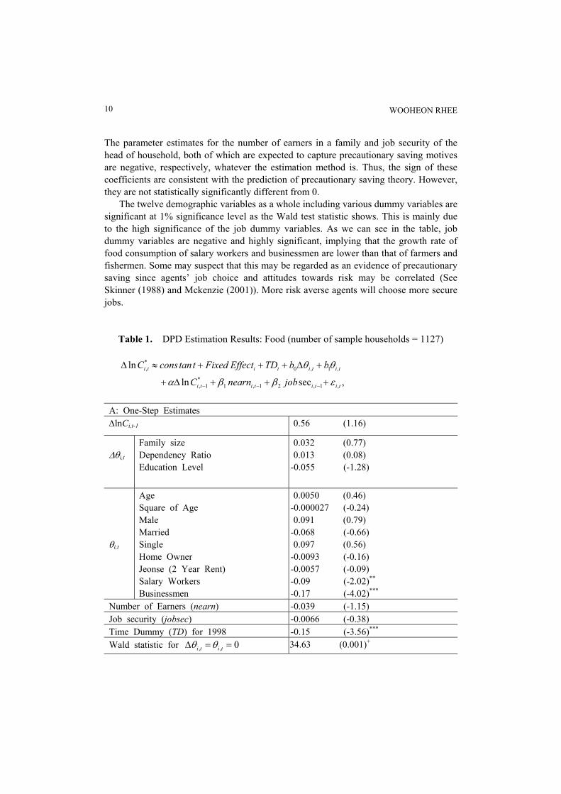
Table 2 reports the DPD estimation results of Equation (14) in the case of nondurables and services consumption. Compared with the results in Table 1, we can find much stronger evidence for both habit formation and precautionary saving in Table 2. Contrary to the results in Table 1, the estimate of the parameter α is now statistically significant at 8 to 11 percent significance levels. One should recall that the estimate α reflects the dominant factor between consumption durability and habit formation. There are some items in our nondurables and services variable that have durability, e.g., shoes. The estimate α can be regarded as a lower bound on the degree of habit formation. Thus from this table, we can find a relatively strong evidence of habit formation in the case of nondurables and services consumption.


Table 2. DPD Estimation Results: Nondurables and Services (number of sample households = 688)

,secln

ln

,1,21,1*

1,

,1,0*,

titititi

titititi

jobnearnC


εββα

θθ

+++∆+

+∆+++≈∆

−−−

A: One-Step Estimates ∆lnCi,t-1 0.58 (1.79)* ∆θi,t


-0.017 (-0.49) 0.36 (2.03)**

-0.028 (-0.95) θi,t


-0.0014 (-0.12) 0.00014 (0.13) 0.086 (0.73)

-0.12 (-1.14) 0.21 (1.12) 0.013 (0.24) 0.028 (0.47)

-0.0062 (-0.16) -0.030 (-0.77)

Number of Earners (nearn) -0.049 (-1.89)* Job security (jobsec) -0.019 (-1.15) Time Dummy (TD) for 1998 -0.22 (-5.49)*** Wald statistic for 0,, ==∆ titi θθ 11.26 (0.51)+ B: One-Step Estimates with Heteroskedasticity-Consistent Standard Errors ∆lnCi,t-1 0.58 (1.62) ∆θi,t


-0.017 (-0.41) 0.36 (1.76)*

-0.028 (-0.78) θi,t


-0.0014 (-0.12) 0.00014 (0.13) 0.086 (0.72)

-0.12 (-1.14) 0.21 (0.73) 0.013 (0.29) 0.028 (0.55)

-0.0062 (-0.15) -0.030 (-0.70)

Number of Earners (nearn) -0.049 (-1.68)* Job security (jobsec) -0.019 (-1.26) Time Dummy (TD) for 1998 -0.22 (-5.52)*** Wald statistic for 0,, ==∆ titi θθ 9.52 (0.66)+

WOOHEON RHEE 14

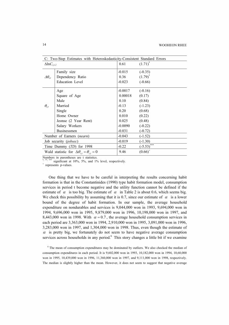
C: Two-Step Estimates with Heteroskedasticity-Consistent Standard Errors ∆lnCi,t-1 0.61 (1.71)*

∆θi,t


-0.015 (-0.35) 0.36 (1.79)*

-0.023 (-0.66)

θi,t


-0.0017 (-0.16) 0.00018 (0.17) 0.10 (0.84)

-0.13 (-1.23) 0.20 (0.68) 0.010 (0.22) 0.025 (0.48)

-0.0090 (-0.22) -0.031 (-0.72)



One thing that we have to be careful in interpreting the results concerning habit formation is that in the Constantinides (1990) type habit formation model, consumption services in period t become negative and the utility function cannot be defined if the estimate of α is too big. The estimate of α in Table 2 is about 0.6, which seems big. We check this possibility by assuming that it is 0.7, since our estimate of α is a lower bound of the degree of habit formation. In our sample, the average household expenditure on nondurables and services is 9,044,000 won in 1993, 9,694,000 won in 1994, 9,696,000 won in 1995, 9,879,000 won in 1996, 10,198,000 won in 1997, and 8,443,000 won in 1998. With 7.0=α , the average household consumption services in each period are 3,363,000 won in 1994, 2,910,000 won in 1995, 3,091,000 won in 1996, 3,283,000 won in 1997, and 1,304,000 won in 1998. Thus, even though the estimate of α is pretty big, we fortunately do not seem to have negative average consumption services across households in any period.6 This story changes a little bit if we examine

6 The mean of consumption expenditures may be dominated by outliers. We also checked the median of consumption expenditures in each period. It is 9,602,000 won in 1993, 10,182,000 won in 1994, 10,60,000 won in 1995, 10,439,000 won in 1996, 11,360,000 won in 1997, and 9,111,000 won in 1998, respectively. The median is slightly higher than the mean. However, it does not seem to suggest that negative average


consumption services of the individual household. With 7.0=α , we have 100 households (14.5% out of 688 households) in 1994, 143 (20.8%) in 1995, 115 (16.7%) in 1996, 113 (16.4%) in 1997, and 223 (32.4%) in 1998, respectively, with negative consumption services. These numbers and percentages drop significantly by almost half if we assume α to be 0.6. Anyway, high estimates of α cause a non-negligible portion of households to suffer from negative consumption services, though it does not cause the average consumption services across households to be negative. These negative consumption services may be explained in part by measurement error in consumption expenditure. Nonetheless, we should note that the number of households with negative consumption services increased dramatically in 1998, when Korea was hit by the Asian currency crisis. This suggests that some households were financially distressed severely in 1998.

Demographic variables as a whole do not seem to be significant in explaining the consumption growth rates of nondurables and services. We cannot reject the hypothesis at conventional significance level that the twelve demographic variables (including dummy variables) are jointly zero. However, the estimate for the dependency ratio is positive and significant at about 4 to 8%. Thus, the growth rate of the nondurables and services consumption seems larger as the dependency ratio increases.

The estimate of the number of earners in a family is again negative. It is now statistically significantly different from 0 at 6 to 13% significance levels depending on the estimation method. This implies that the evidence of precautionary saving is relatively stronger in the case of nondurables and services consumption than in the case of food consumption. Again, the time dummy for 1998 has negative value and is highly statistically significant. However, the estimate of job security of the head of household is still not statistically significant, even though it is negative. Furthermore, the coefficient of the dummy variable for home owners is positive, though it is not significant. These are evidence against the precautionary saving theory. Thus, it would be fair to say that the evidence of precautionary saving is mixed in the case of nondurables and services consumption.

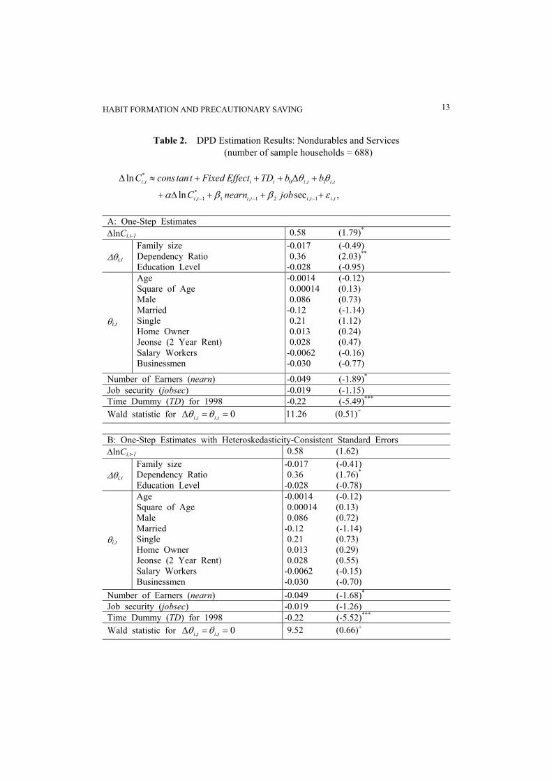
One may suspect that the job security evaluated by the head of household does not exactly reflect the descending order of uncertainty declining by equal magnitude, and so, it might be better to use dummies instead of using the variable directly. Furthermore, we may expect that the precautionary saving motive is most strong for the household with very insecure job security relative to other households. Another thing we also have to note is that job security may be related to job dummy variables as discussed in Table 1. This correlation may reduce the significance of job security in the regression. In order to take care of these problems we include a dummy variable for the household with very insecure job in the regression instead of using job security variable itself.

consumption services across households are a serious possibility on average across households.

WOOHEON RHEE 16

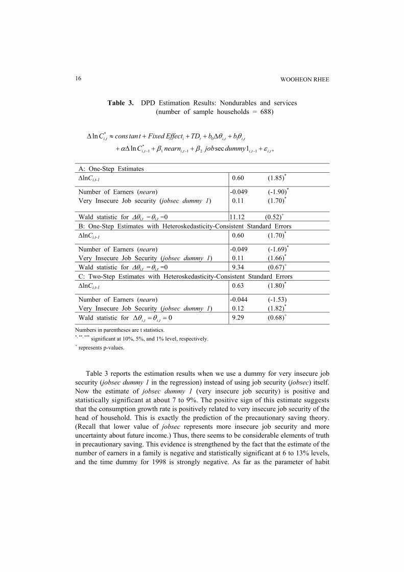
Table 3. DPD Estimation Results: Nondurables and services (number of sample households = 688)

,1secln

ln

,1,21,1*

1,

,1,0*,

titititi

titititi

dummyjobnearnC


εββα

θθ

+++∆+

+∆+++≈∆

−−−

A: One-Step Estimates ∆lnCi,t-1 0.60 (1.85)*

Number of Earners (nearn) Very Insecure Job security (jobsec dummy 1)

-0.049 (-1.90)* 0.11 (1.70)*

Wald statistic for ∆θi,t =θi,t =0 11.12 (0.52)+ B: One-Step Estimates with Heteroskedasticity-Consistent Standard Errors ∆lnCi,t-1 0.60 (1.70)*

Number of Earners (nearn) Very Insecure Job Security (jobsec dummy 1)

-0.049 (-1.69)* 0.11 (1.66)*

Wald statistic for ∆θi,t =θi,t =0 9.34 (0.67)+ C: Two-Step Estimates with Heteroskedasticity-Consistent Standard Errors ∆lnCi,t-1 0.63 (1.80)*

Number of Earners (nearn) Very Insecure Job Security (jobsec dummy 1)

-0.044 (-1.53) 0.12 (1.82)*

Wald statistic for 0,, ==∆ titi θθ 9.29 (0.68)+


Table 3 reports the estimation results when we use a dummy for very insecure job

security (jobsec dummy 1 in the regression) instead of using job security (jobsec) itself. Now the estimate of jobsec dummy 1 (very insecure job security) is positive and statistically significant at about 7 to 9%. The positive sign of this estimate suggests that the consumption growth rate is positively related to very insecure job security of the head of household. This is exactly the prediction of the precautionary saving theory. (Recall that lower value of jobsec represents more insecure job security and more uncertainty about future income.) Thus, there seems to be considerable elements of truth in precautionary saving. This evidence is strengthened by the fact that the estimate of the number of earners in a family is negative and statistically significant at 6 to 13% levels, and the time dummy for 1998 is strongly negative. As far as the parameter of habit


formation is concerned, it is estimated to be about 0.6 and statistically significantly different from 0 at 6 to 9% levels.

In summary, using the KHPS, we found that the estimates of parameters corresponding to the degree of habit formation and precautionary saving are statistically insignificant for food consumption, but statistically significant or, to say the least, marginally significant for nondurables and services consumption.

5. CONCLUSIONS In this paper, we examined the evidence of precautionary saving and Constantinides

(1990) type habit formation model in a single framework by using the Korean Household Panel Studies. If consumption shows habit formation, consumption expenditure in the previous period is a complement to consumption expenditure today. Then, the regression coefficient for the consumption growth rate on the one-period lagged consumption growth rate is expected to be positive. In addition, we examined the evidence of precautionary saving by employing the number of earners in a family and job security evaluated by the head of household as variables that are expected to capture various precautionary saving channels. If there are more earners in a family, there will be less risk of catastrophic drop in family income, and there will be less incentive for precautionary saving. Similarly, we expect that as the uncertainty faced by a household decreases, there is less incentive for precautionary saving. Employing the dynamic panel data estimation method, we found that the estimates of parameters corresponding to the degree of habit formation and precautionary saving are statistically insignificant for food consumption, but statistically significant or at least marginally significant for nondurables and services consumption.

In interpreting the results, we should take the following facts into consideration; First, our estimate of habit formation actually reflects the dominant force between habit formation and consumption durability. Some items in our nondurables and services show durability and our estimate can be regarded as a lower bound on the degree of habit formation. Second, our measures that are expected to capture various precautionary saving motives, that is, number of earners in a family and job security of the head of household, are not perfect in capturing uncertainty about future income. That may be why we could not detect stronger evidence of precautionary saving in the data.

One more caveat: Before we draw any strong conclusions about the evidence of habit formation, we should recall that the model we examined in this paper is just one of several models developed recently. It is hasty to say something strong about the evidence of habit formation before we examine empirical evidence of different models of habit formation, for example, such as Campbell and Cochrane’s (1999) and Abel’s (1990).

WOOHEON RHEE 18

REFERENCES Abel, A.B. (1990), “Asset Prices under Habit Formation and Catching Up with the

Joneses,” American Economic Review 40, pp. 38-42. Arellano, M., and S. Bond (1991), “Some Tests of Specification for Panel Data: Monte

Carlo Evidence and an Application to Employment Equations,” Review of Economic Studies 58, pp. 277-297.

_____ (1998), “Dynamic Panel Data Estimation Using DPD98 for GAUSS: A Guide for Users,” manuscript 6.

Attanasio, O.P. (1998), “Consumption Demand,” NBER WP #6466. Blundell, R., and S. Bond (1998), “Initial Conditions and Moment Restrictions in

Dynamic Panel Data Models,” Journal of Econometrics 87, pp. 115-143. Campbell, J.Y., and J.H. Cochrane (1999), “By Force of Habit: A Consumption-Based

Estimation of Aggregate Stock Market Behavior,” Journal of Political Economy 107, pp. 205-251.

Carroll, C.D., and L.H. Summers (1991), “Consumption Growth Parallels Income Growth: Some New Evidence,” in B. Douglas Bernheim and John B. Shoven, eds., National Saving and Economic Performance, University of Chicago Press, pp. 305-343.

Christiano, L.J., M. Eichenbaum, and D. Marshall (1991), “The Permanent Income Hypothesis Revisited,” Econometrica 59, pp. 397-423.

Constantinides, G.M. (1990), “Habit Formation: A Resolution of the Equity Premium Puzzle,” Journal of Political Economy 98, pp. 519-543.

Deaton, A. (1992), Understanding Consumption, Clarendon Lectures in Economics, Oxford University.

Dynan, K.E. (2000), “Habit Formation in Consumer Preferences: Evidence from Panel Data,” American Economic Review 90, pp. 391-406.

Hayashi, F. (1985), “The Permanent Income Hypothesis and Consumption Durability: Analysis Based on Japanese Panel Data,” Quarterly Journal of Economics 100, pp. 1083-1113.

McKenzie, D. (2001), “Consumption Growth in a Booming Economy: Taiwan 1976-96,” Economic Growth Center, Yale University, Discussion Paper #823.

Muellbauer, J. (1988), “Habits, Rationality and Myopia in the Life-Cycle Consumption Function,” Annales d’Economie et de Statistique 9, pp. 47-70.

Skinner, J. (1988), “Risky Income, Life Cycle Consumption, and Precautionary Savings,” Journal of Monetary Economics 22, pp. 237-255.

Working, H. (1960), “Note on the Correlation of First Differences of Averages in a Random Chain,” Econometrica 28, pp. 916-18.

Zeldes, S.P. (1989), “Consumption and Liquidity Constraints: An Empirical Investigation,” Journal of Political Economy 97, pp. 305-346.


Mailing Address: Department of Economics, Kyunghee University, Seoul, Korea. Tel: 82-2-961-0774, Fax: 82-2-966-7426. E-mail: [email protected]

Manuscript received Febrnary, 2004; final revision received July, 2004.

habit formation and precautionary saving: evidence from the korean

Documents