Paulo Jorge Baeta Mendes

H-O (H-N) COMPLEXES IN METALS, STUDIED BY PERTURBED ANGULAR

CORRELATIONS

University of Coimbra1987

INDEX

ABSTRACT . . . . . . . . . . . . . . . . . . . . . . . . . . . . . . . 3Acknowledgements . . . . . . . . . . . . . . . . . . . . . . . . . . . . 4

Chapter 1. - INTRODUCTION . . . . . . . . . . . . . . . . . . . . 51.1 - The project . . . . . . . . . . . . . . . . . . . . . . . . . . 51.2 - Plan of thesis . . . . . . . . . . . . . . . . . . . . . 7

Chapter 2. - THEORECTICAL CONSIDERATIONS . . . . . . . . . . 92.1 - Hyperfine interactions . . . . . . . . . . . . . . . . . . . . . 92.2 - The perturbed angular correlation . . . . . . . . . . . . . . 102.3 - The electric quadrupole interaction . . . . . . . . . . . . . . 132.4 - The probe nucleus . . . . . . . . . . . . . . . . . . . . . . . . 152.5 - The point charge model . . . . . . . . . . . . . . . . . . . . 17

Chapter 3. - EXPERIMENTAL . . . . . . . . . . . . . . . . . . . . . 203.1 - The experimental system . . . . . . . . . . . . . . . . . . . 203.1.1 - Detectors and electronics . . . . . . . . . . . . . . . . . . 203.1.2 - Criostat and temperature control . . . . . . . . . . . . . . 263.2 - Sample preparation . . . . . . . . . . . . . . . . . . . . . . . 273.2.1 - Probe atom dilution . . . . . . . . . . . . . . . . . . . . . . 273.2.2 - Nitrogen and oxygen dilution . . . . . . . . . . . . . . . . 303.2.3 - Hydrogen and deuterium dilution . . . . . . . . . . . . . 313.2.4 - Hydrogen and deuterium concentration determination . . . . 313.3 - Data analysis . . . . . . . . . . . . . . . . . . . . . . . . . . 333.3.1 - The perturbation factor extracted from the time spectra 333.3.2 - R(t) fitting . . . . . . . . . . . . . . . . . . . . . . . . . . . 383.3.3 - The Fourier transform . . . . . . . . . . . . . . . . . . . . . 40

Chapter 4. - OXYGEN AND NITROGEN STUDIES IN TANTALUM AND NIOBIUM . . . . . . . . . . . . . . . . . . . 414.1 - Experimental results . . . . . . . . . . . . . . . . . . . . . . 424.1.1 - The Ta-O system . . . . . . . . . . . . . . . . . . . . . . . . 424.1.2 - The Ta-N system . . . . . . . . . . . . . . . . . . . . . . . . 434.1.3 - The Nb-O system . . . . . . . . . . . . . . . . . . . . . . . 434.1.4 - The Nb-N system . . . . . . . . . . . . . . . . . . . . . . . 434.2 - Discussion . . . . . . . . . . . . . . . . . . . . . . . . . . . . 474.2.1 - The interaction frequencies νQ . . . . . . . . . . . . . . . � 48

4.2.2 - The asymmetry parameters η . . . . . . . . . . . . . . . . . �50

4.2.3 - The temperature dependence of νQ e η . . . . . . . . . . . �53

4.3 - Conclusions . . . . . . . . . . . . . . . . . . . . . . . . . . . 54

1

Chapter 5. - STUDIES OF THE INTERACTION OF HYDROGEN AND DEUTERIUM WITH OXYGEN AND NITROGEN IN TANTALUM AND NIOBIUM . . . . . . . . . . . . . 565.1 - Introduction . . . . . . . . . . . . . . . . . . . . . . . . . . . 565.2 - Experimental results . . . . . . . . . . . . . . . . . . . . . . 585.2.1 - The Ta-O-H(D) system . . . . . . . . . . . . . . . . . . . . . 595.2.2 - The Ta-N-H(D) system . . . . . . . . . . . . . . . . . . . . . 595.2.3 - The Nb-O-H(D) system . . . . . . . . . . . . . . . . . . . . 625.3 - Discussion . . . . . . . . . . . . . . . . . . . . . . . . . . . 685.3.1 - Assignment of the interaction frequencies νQ . . . . . . . � 68

5.3.2 - The asymmetry parameters η . . . . . . . . . . . . . . . � 725.3.3 - Temperature dependence of the defect fractions . . . . . . 755.3.3.a - Classical thermodynamical equilibrium . . . . . . . . . . 755.3.3.b - Thermodynamical equilibrium with trapped hydrogen . . . . . . . . . . . . . . . . . . . . . . . . 805.3.3.c - Hydrogen released by the nuclear decay . . . . . . . . . . 835.4 - Conclusions . . . . . . . . . . . . . . . . . . . . . . . . . . 88

Chapter 6. - FINAL REMARKS . . . . . . . . . . . . . . . . . . . . . 90

APPENDIXES:

APPENDIX A. - THE PERTURBED ANGULAR CORRELATION AND THE ELECTRIC HYPERFINE INTERACTION . . 92A.1 - The perturbed angular correlation . . . . . . . . . . . . . 92A.2 - The electric quadrupole interaction . . . . . . . . . . . . . 96A.2.1 - Classical hyperfine interaction . . . . . . . . . . . . . . . 96A.2.2 - Quantum treatment of the electric quadrupole interaction . . . . . . . . . . . . . . . . . . . . . . . 98A.2.3 - The perturbation factor for the electric quadrupole interaction . . . . . . . . . . . . . . . . . . . . . . . 103

APPENDIX B. - THE DATA ACQUISITION SYSTEM DEVELOPED IN COIMBRA . . . . . . . . . . . . . . . . . . . . . . . . . . . . . . 106B.1 - The digital router . . . . . . . . . . . . . . . . . . . . . . . 108

REFERENCES. . . . . . . . . . . . . . . . . . . . . . . . . . . . . 110

2

A B S T R A C T

Studies of the interaction of hydrogen and deuterium with the interstitial impurities oxygen and nitrogen in niobium and tantalum were performed using the perturbed angular correlation technique with 181Hf as probe atom.

The interactions due to oxygen and nitrogen in these metals were identified and their evolution as a function of temperature was studied. For oxygen in niobium and tantalum and for nitrogen in tantalum no complexes of more than one interstitial atom were observed for the low concentrations studied. However two different types of complexes were observed for nitrogen in niobium which were attributed to the loading method used for this interstitial.

The relative values of the interaction parameters are interpreted in terms of the va-lence charge distribution of the impurities. The largest temperature dependence of the asymmetry parameter η in niobium is justified by the fact that the 181Ta atom where the angular correlation is observed is an impurity in niobium whereas in tantalum is similar to the lattice atoms.

The interactions due to oxygen-hydrogen complexes in tantalum and niobium and to nitrogen-hydrogen complexes in tantalum were also identified and their evolution with temperature studied. Similar interactions are observed when deuterium is used instead of hydrogen.

The use of this method confirms that only one hydrogen atom is captured by oxy-gen or nitrogen in these metals. Using a simple point charge model it was also possi-ble to confirm the position of the trapped hydrogen atom at two neighbouring tetrahe-dral positions which are fourth nearest neighbours to the oxygen or nitrogen atoms. The probe atom, which is an impurity in these metals, plays an important role on the behaviour of the complexes studied lowering the temperature at which the interactions due to these complexes disappear.

A trapping model in which after the decay of hafnium hydrogen is released and diffuses around the trapping impurity is presented. The values for the mean time of stay of hydrogen obtained with this model lie between those predicted by an extrapo-lation of the Arrhenius behaviour of the experimental values for the pure metal and for the metal with oxygen or nitrogen as impurities.

3

A C K N O W L E D G E M E N T S

The present work was made possible only by the encouragement and support of all the members of the Applied Nuclear Physics Group, part of Linha 2 of the Centro de Física da Radiação e dos Materiais of the University of Coimbra, whose creation is due to Prof. Doutor Nuno Ayres de Campos with the collaboration of Prof. Doutor Adriano Pedroso de Lima.

I wish to express my gratitude especially to the following:

Prof. Doutor Nuno Ayres de Campos who selected the research theme and for his constant support and continuous encouragement and friendship,

Prof. Doutor Adriano Pedroso de Lima for his support throughout the work and for his patient and careful reading of the text.,

Prof. Doctor Eckehard Recknagel for granting me access to all the facilities of his laboratory in the Physics Department of the University of Konstanz,

Prof. Doctor Alois Weidinger for his invaluable help in the development of the re-search and for helpful discussions throughout the work,

Prof. Doutor José Carvalho Soares for the use of his facilities in Lisboa for some low temperature measurements,

to my colleagues in Coimbra, Konstanz and Lisboa,Deutscher Akademischer Austauschdienst (D.A.A.D.) and the Instituto Nacional de

Investigação Científica (I.N.I.C.) for their financial support.

4

CHAPTER 1

INTRODUCTION

1.1 - The project

This work is the first application of the perturbed angular correlation

technique to the study of complexes of hydrogen trapped at interstitial im-

purities in metallic lattices. The study of these complexes is of great impor-

tance particularly in hydrogen diffusion studies in metals. Hydrogen diluted

in a perfect metallic lattice has properties similar to those of a gas with a gas

phase (α phase), a liquid phase (α‘ phase) and ordered solid phases which

depend on temperature as well as hydrogen concentration. The amount of

hydrogen which remains in the α phase when the temperature is lowered is

drastically reduced due to precipitations in ordered phases. For this reason

diffusion measurements at low temperatures are extremely difficult to per-

form and the diffusion coefficients for hydrogen and it’s isotopes are only

known above 120K. A large number of experimental studies have shown

that at low temperatures oxygen and nitrogen are good trapping centers for

hydrogen in niobium and tantalum. The trapping of hydrogen by nitrogen

in niobium has been particularly well studied [Pfeiffer 76, Chen 76, Hanada

77 and 81a, Sado 82, Okuda 84] using methods such as electrical resistivity

5

and internal friction. It was found that for these systems and at low tem-

peratures N-H (or O-H) complexes are formed while trapping centers are

available and that the excess hydrogen atoms precipitate. The internal fric-

tion relaxation peaks observed suggest that hydrogen diffuses around nitro-

gen or oxygen trap centers. This shows that the study of hydrogen diffusion

processes at low temperatures is possible by studying it’s local diffusion

around immobile trap centers as long as the binding energy between hydro-

gen and the trapping center is high enough to prevent precipitation.

The local diffusion of hydrogen in O-H and N-H complexes in niobium

and tantalum has been studied by internal friction [Baker 73, Mattas 75,

Schiller 75, Poker 79, Zapp 80a and 80], heat capacity [Morkel 78, Wipf 84],

thermal conductivity [Locattelli 78] and neutron spectroscopy [Wipf 81,

Magerl 83 e 86]. This studies suggest that hydrogen is located at two neigh-

bouring lattice positions (tetrahedral or quasi-tetrahedral) jumping between

them by tunneling. Both oxygen and nitrogen are located at octahedral in-

terstitial positions in niobium and tantalum and the most likely positions

for trapped hydrogen is in the pair of tetrahedral positions which are 4th

nearest neighbours (4NN) to oxygen or nitrogen. When the temperature is

increased hydrogen diffuses around the trapping center jumping to the

other 4NN possible positions. If the energy available is enough then hydro-

gen moves away from the impurity and diffuses through the metal.

Microscopic methods such as perturbed angular correlations overcome

some of the limitations of the refered macroscopic methods. It´s local char-

acter (defects which are more than three or four unit cells away from the

probe are not detected) allows an easy distinction between different types of

defects and even between different configurations of the same defect. With

this technique measurements of the mean time of residence of hydrogen in

6

tantalum at temperatures below 30K were first performed by Weidinger and

Peichl [Weidinger 85].

In the present work the perturbed angular correlation technique was

used to study the trapping and local diffusion of hydrogen and deuterium

around oxygen and nitrogen in niobium and tantalum.

1.2 - Plan of thesis

Some of the fundamental aspects of the perturbed angular correlation

method used in this work are presented in chapter 2. A summary of the

theory of angular correlations and of the hyperfine interaction between the

nuclear quadrupole moment and the external electric field gradient is pre-

sented in appendix A. The properties of the nuclear probe used as well as

the point charge model for electric field gradient calculation are also pre-

sented.

In chapter 3 the experimental systems and the methods used to dilute

the probe atoms, oxygen, nitrogen, hydrogen and deuterium are described.

The hydrogen concentration measurement system developed is also dis-

cussed as well as the numerical methods used in the data analysis. In ap-

pendix B the data acquisition system developed in Coimbra is presented.

The studies of oxygen and nitrogen interactions in niobium and tanta-

lum are presented in chapter 4. The interactions observed are identified and

the temperature dependence of their parameters are discussed for the dif-

ferent systems. At the end of this chapter a summary of the relevant conclu-

sions is made.

The results of the studies of the interaction of hydrogen with oxygen

and nitrogen in tantalum and with oxygen in niobium are presented in

7

chapter 5. The different interactions present are identified and the depend-

ence on temperature of the fraction of trapped hydrogen atoms s inter-

preted in terms of trapping models. The limitations of several models are

discussed and a summary of conclusions is presented at the end of the

chapter.

Finally in chapter 6 some final remarks are made and future develop-

ments are suggested.

8

CHAPTER 2

THEORETICAL CONSIDERATIONS

2.1 - Hyperfine interactions

The interaction of the nuclear charge distribution with the electromag-

netic fields produced either by the atomic electrons or by the crystal

charges, hyperfine interactions, induce changes in the nuclear and atomic

energy levels. The hyperfine interaction Hamiltonian may be conveniently

written in terms of a multipolar expansion:

Hhi = H (E0) + H (M1) + H (E2) + ... (2.1)

where H(E0) is the electric monopole term, H(M1) is the magnetic dipole

term, H(E2) is the electric quadrupole term, etc. and correspond to the nu-

clear moments which do not vanish due to symmetries of the nuclear states.

Each term of the expansion of Hhi may be written as a product of a nu-

clear moment and a corresponding electromagnetic moment. Therefore hy-

perfine interaction studies give information concerning nuclear moments or

crystal fields. However the experimental determination of either of the two

terms requires a detailed knowledge of the other.

Studies of hyperfine interactions may be carried out by several methods

wether in ground states of stable nuclei, or with half-lives of the order of

several minutes (high resolution optical spectroscopy, nuclear magnetic

9

resonance(NMR)), or in nuclear excited states (Mössbauer spectroscopy, per-

turbed angular correlations (PAC)). These last methods use nuclear radia-

tion to detect the hyperfine interaction and are nowadays considered as

very powerful tools in different research fields such as Solid State Physics,

Chemistry and even Biology.

In the perturbed angular correlation method used in this work the hy-

perfine interaction between the nuclear quadrupole moment and the elec-

tric field gradient due to the atomic and crystalline charge distribution is

studied. The general theory of angular correlations and hyperfine interac-

tions is well known and only a brief summary is presented in Appendix A.

2.2 - The perturbed angular correlation

The perturbed angular correlation method consists basically in obtain-

ing an ensemble of aligned nuclei in an excited state and measuring the an-

gular distribution of the radiation emitted from this state. Alignment of an

ensemble of nuclei is obtained when the population of different magnetic

sub-states are not equal but states with symmetric magnetic quantum num-

bers, ± m, are equally populated.

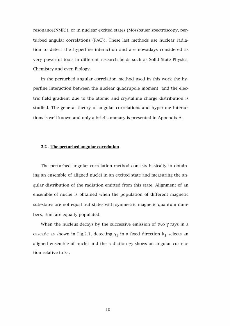
When the nucleus decays by the successive emission of two γ rays in a

cascade as shown in Fig.2.1, detecting γ1 in a fixed direction k1 selects an

aligned ensemble of nuclei and the radiation γ2 shows an angular correla-

tion relative to k1.

10

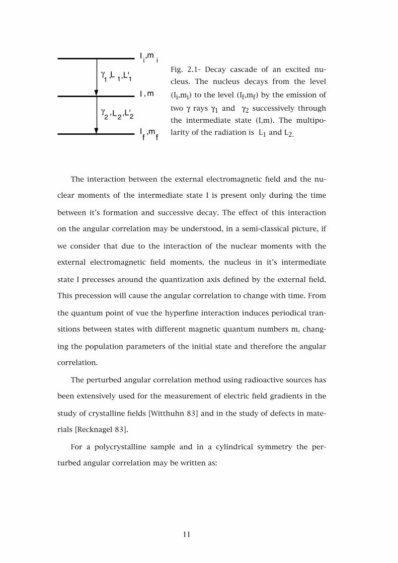
Fig. 2.1- Decay cascade of an excited nu-cleus. The nucleus decays from the level

(Ii,mi) to the level (If,mf) by the emission of

two γ rays γ1 and γ2 successively through the intermediate state (I,m). The multipo-larity of the radiation is L1 and L2.

The interaction between the external electromagnetic field and the nu-

clear moments of the intermediate state I is present only during the time

between it’s formation and successive decay. The effect of this interaction

on the angular correlation may be understood, in a semi-classical picture, if

we consider that due to the interaction of the nuclear moments with the

external electromagnetic field moments, the nucleus in it’s intermediate

state I precesses around the quantization axis defined by the external field.

This precession will cause the angular correlation to change with time. From

the quantum point of vue the hyperfine interaction induces periodical tran-

sitions between states with different magnetic quantum numbers m, chang-

ing the population parameters of the initial state and therefore the angular

correlation.

The perturbed angular correlation method using radioactive sources has

been extensively used for the measurement of electric field gradients in the

study of crystalline fields [Witthuhn 83] and in the study of defects in mate-

rials [Recknagel 83].

For a polycrystalline sample and in a cylindrical symmetry the per-

turbed angular correlation may be written as:

γ1 ,

I i,i m

I ,m

I ,fmf

L 1,L'1

2γ , 2L ,L'2

11

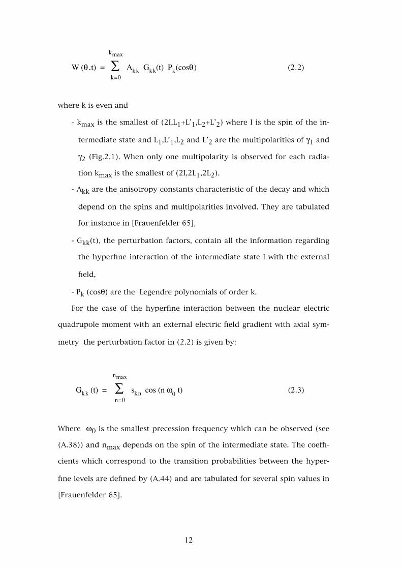
W (θ, t) = ∑k=0

kmax

Akk Gkk(t) Pk(cosθ) (2.2)

where k is even and

- kmax is the smallest of (2I,L1+L’1,L2+L’2) where I is the spin of the in-

termediate state and L1,L’1,L2 and L’2 are the multipolarities of γ1 and

γ2 (Fig.2.1). When only one multipolarity is observed for each radia-

tion kmax is the smallest of (2I,2L1,2L2).

- Akk are the anisotropy constants characteristic of the decay and which

depend on the spins and multipolarities involved. They are tabulated

for instance in [Frauenfelder 65],

- Gkk(t), the perturbation factors, contain all the information regarding

the hyperfine interaction of the intermediate state I with the external

field,

- Pk (cosθ) are the Legendre polynomials of order k.

For the case of the hyperfine interaction between the nuclear electric

quadrupole moment with an external electric field gradient with axial sym-

metry the perturbation factor in (2.2) is given by:

Gkk (t) = ∑n=0

nmax

skn cos (n ω0 t) (2.3)

Where ω0 is the smallest precession frequency which can be observed (see

(A.38)) and nmax depends on the spin of the intermediate state. The coeffi-

cients which correspond to the transition probabilities between the hyper-

fine levels are defined by (A.44) and are tabulated for several spin values in

[Frauenfelder 65].

12

When the electric field gradient is not axial symmetric the transition

probabilities and energies are a function of the asymmetry parameter η

(defined below) and the perturbation factor becomes:

Gkk (t) = ∑n=0

nmax

skn(η) cos (nn(η) ω0 t) (2.4)

where nn(η) is the ratio between the experimental frequencies, ωn, and the

frequency w0 for η=0.

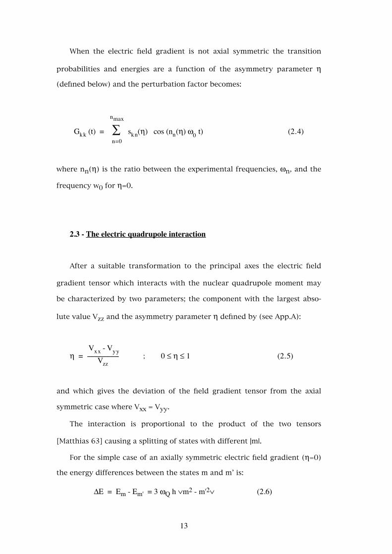
2.3 - The electric quadrupole interaction

After a suitable transformation to the principal axes the electric field

gradient tensor which interacts with the nuclear quadrupole moment may

be characterized by two parameters; the component with the largest abso-

lute value Vzz and the asymmetry parameter η defined by (see App.A):

η = ------------------------ Vxx - Vyy

Vzz ; 0 ≤ η ≤ 1 (2.5)

and which gives the deviation of the field gradient tensor from the axial

symmetric case where Vxx = Vyy.

The interaction is proportional to the product of the two tensors

[Matthias 63] causing a splitting of states with different |m|.

For the simple case of an axially symmetric electric field gradient (η=0)

the energy differences between the states m and m’ is:

ΔE = Em - Em' = 3 ωQ h ∨m2 - m'2∨ (2.6)

13

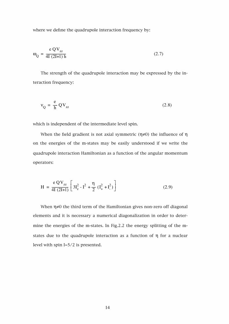
where we define the quadrupole interaction frequency by:

ωQ = --------------------------e Q Vzz

4I (2I+1) h (2.7)

The strength of the quadrupole interaction may be expressed by the in-

teraction frequency:

νQ = ------eh Q Vzz (2.8)

which is independent of the intermediate level spin.

When the field gradient is not axial symmetric (η≠0) the influence of η

on the energies of the m-states may be easily understood if we write the

quadrupole interaction Hamiltonian as a function of the angular momentum

operators:

H = ----------------------e Q Vzz

4I (2I+1) ⎢⎡⎣ ⎥

⎤⎦3Iz

2 - I2 + ------η2 ( )I+

2 + I-2 (2.9)

When η≠0 the third term of the Hamiltonian gives non-zero off diagonal

elements and it is necessary a numerical diagonalization in order to deter-

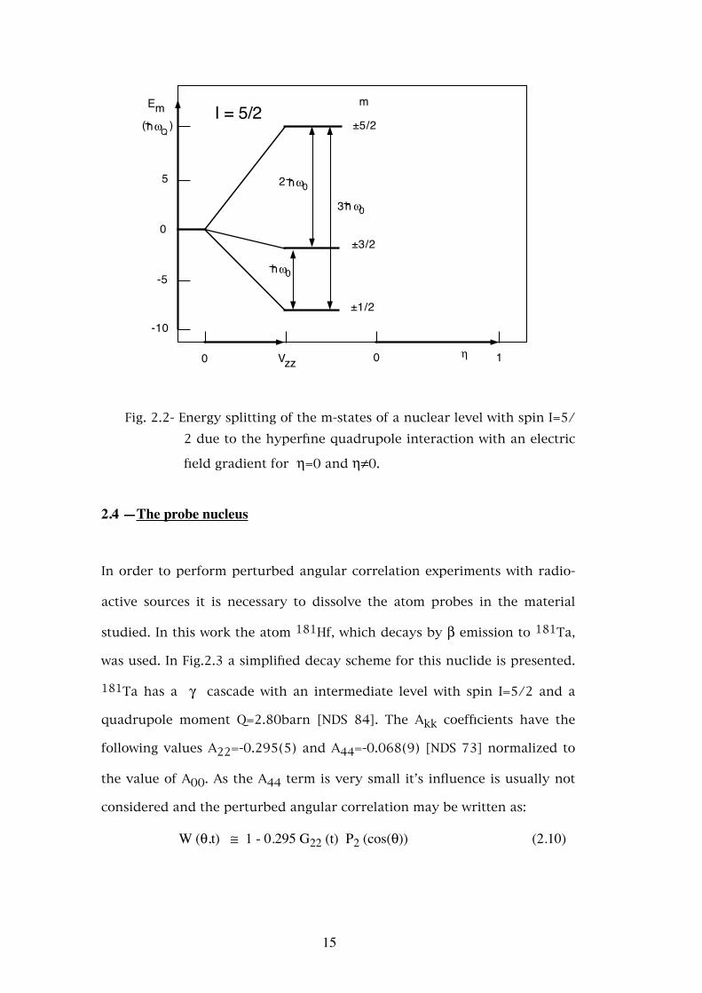
mine the energies of the m-states. In Fig.2.2 the energy splitting of the m-

states due to the quadrupole interaction as a function of η for a nuclear

level with spin I=5/2 is presented.

14

±5/2

±3/2

±1/2

mmE

Vzz

hωQ( )

hω02

hω03

hω0

I = 5/2

5

0

-5

-10

0 0 1η

Fig. 2.2- Energy splitting of the m-states of a nuclear level with spin I=5/2 due to the hyperfine quadrupole interaction with an electric

field gradient for η=0 and η≠0.

2.4 —The probe nucleus

In order to perform perturbed angular correlation experiments with radio-

active sources it is necessary to dissolve the atom probes in the material

studied. In this work the atom 181Hf, which decays by β emission to 181Ta,

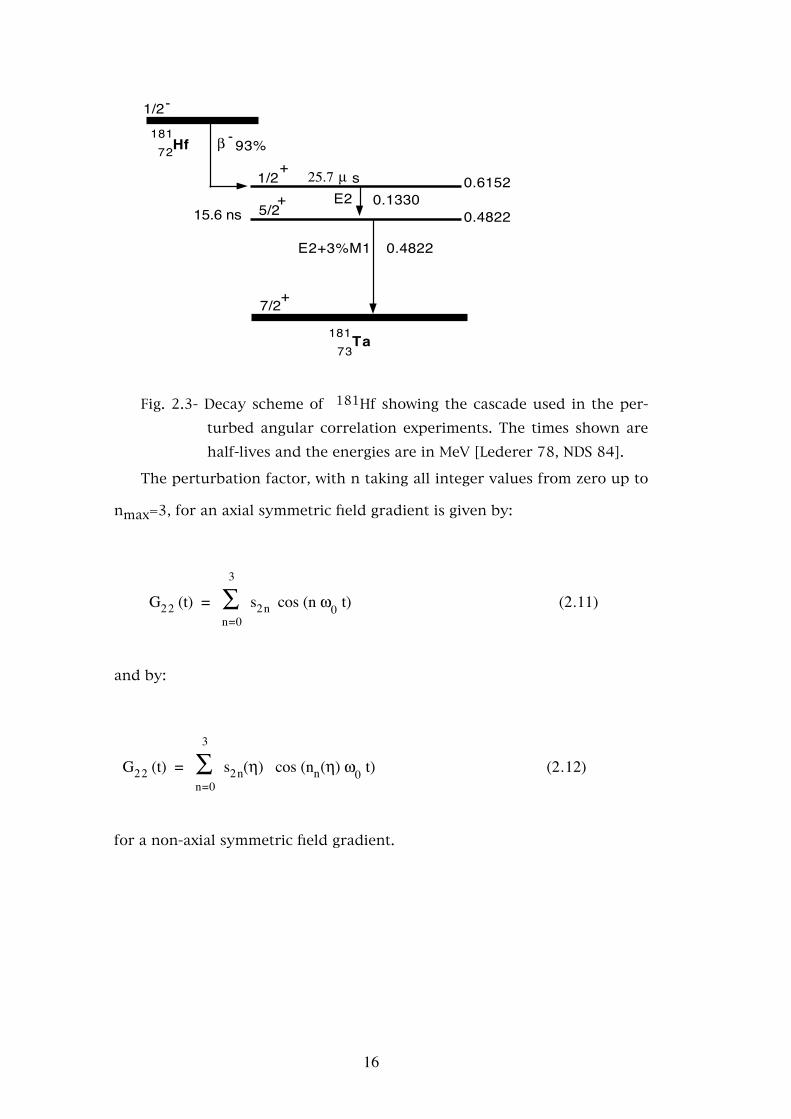
was used. In Fig.2.3 a simplified decay scheme for this nuclide is presented.

181Ta has a γ cascade with an intermediate level with spin I=5/2 and a

quadrupole moment Q=2.80barn [NDS 84]. The Akk coefficients have the

following values A22=-0.295(5) and A44=-0.068(9) [NDS 73] normalized to

the value of A00. As the A44 term is very small it’s influence is usually not

considered and the perturbed angular correlation may be written as:

W (θ,t) ≅ 1 - 0.295 G22 (t) P2 (cos(θ)) (2.10)

15

181Hf72

181Ta73

1/2-

1/2+

+5/2

+7/2

β - 93%

25.7 µ s

15.6 nsE2

E2+3%M1

0.6152

0.48220.1330

0.4822

Fig. 2.3- Decay scheme of 181Hf showing the cascade used in the per-turbed angular correlation experiments. The times shown are half-lives and the energies are in MeV [Lederer 78, NDS 84].

The perturbation factor, with n taking all integer values from zero up to

nmax=3, for an axial symmetric field gradient is given by:

G22 (t) = ∑n=0

3

s2n cos (n ω0 t) (2.11)

and by:

G22 (t) = ∑n=0

3

s2n(η) cos (nn(η) ω0 t) (2.12)

for a non-axial symmetric field gradient.

16

2.5 - The point charge model

As the theoretical determination of the electric field gradient in a metal

requires a detailed knowledge of the electronic wave functions of the crystal

it is not possible to calculate it exactly even for the simplest metals. The

theoretical methods developed for these calculations are usually based in

approximations depending on the particular metal in study which difficults

their application to other metals.

Furthermore these studies have usually been concentrated in non-cubic

metals [Kaufman 79, Vianden 83] and on the calculation of field gradients

caused by substitutional impurities in cubic metals at their nearest neigh-

bours [Ponnambalam 84,85, Pal 85, Prakash 85]. Theoretical studies of elec-

tric field gradients caused by interstitial impurities in cubic metals are prac-

tically non-existent.

Usually two contributions to the electric field gradient are considered,

one is due to the electronic charge density outside the atom used as probe

and the second is due to non-spherical charge distributions belonging to the

probe atom:

Vzz = (1-γ∞) VzzExt + (1-R) Vzz

Loc (2.13)

The Sternheimer anti-shielding factor γ∞ gives the enhancement of the field

gradient at the nucleus due to the polarization of the probe nucleus elec-

tronic shells by the external field gradient. This factor is negative for most

ions and has usually values in the range 10 ≤- γ∞ ≤ 80 [Feiock 69]. R is the

shielding factor for the local gradient and has usually values in the range

-0.2≤R≤0.2 [Kaufmann 79].

17

As refered above theoretical calculations of electric field gradients use

rather elaborate models that are specific for each metal studied. With the

use of models the identification of defect configurations is, in principle, pos-

sible by comparing the experimental results with the theoretical calcula-

tions. However due to the fact that each model must be adapted to the type

of defect considered and that the field gradient has to be calculated for all

possible defect configurations, these calculations are not feasible from the

practical point of vue.

These difficulties have led to the use of a very simple, although rather

unrealistic, model for the determination of the electric field gradient; the

point charge model. In this model the crystal charge distribution is replaced

by point charges placed at the equilibrium lattice points and the field gradi-

ent is calculated using this charge distribution. The so called lattice contri-

bution to the electric field gradient, (1- γ∞)VzzRede, which is often used in-

stead of the first term in (2.13). This value is usually much different from

the experimental values. This difference is often attributed to local gradients

included on the second term of (2.13). In spite of it’s simplicity this model

has been successfully used to predict the symmetry of field gradients in the

presence of impurities [Weidinger 79, Wrede 86]. An improved version of

this model where the crystal electronic charge distribution is also replaced

by negative point charges placed in points where this density is greater is

sometimes used [Bodenstedt 85, Gil 87b].

In the point charge model the electric field gradient tensor created by

the charge distribution external to the probe atom is calculated from the

second derivatives of the electrostatic potential:

VαβRede = -----------------

∂2V∂x

α∂x

β (2. 14)

18

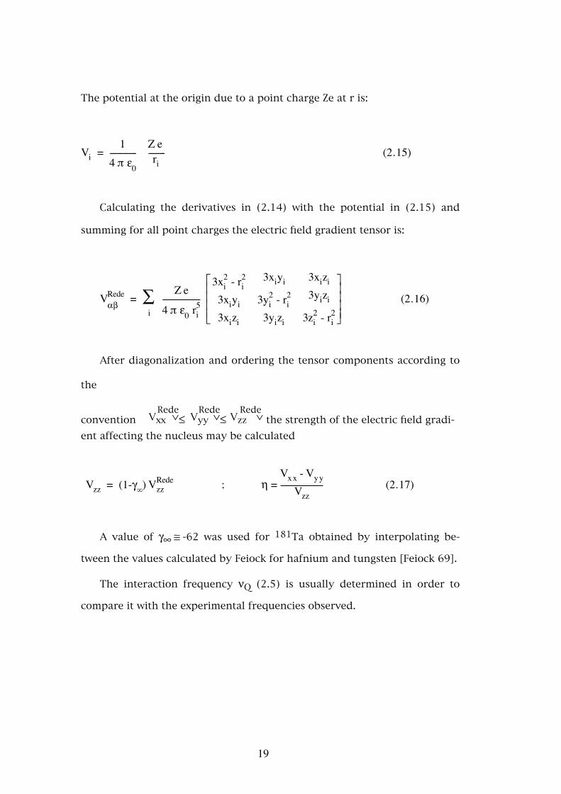
The potential at the origin due to a point charge Ze at r is:

Vi = --------------1

4 π ε0

---------Z e ri

(2.15)

Calculating the derivatives in (2.14) with the potential in (2.15) and

summing for all point charges the electric field gradient tensor is:

VαβRede = ∑

i --------------------

Z e

4 π ε0 ri5 ⎢⎢⎢⎢

⎡

⎣

⎥⎥⎥⎥

⎤

⎦

3xi2 - ri

2

3xiyi3xizi

3xiyi

3yi2 - ri

2

3yizi

3xizi3yizi

3zi2 - ri

2 (2.16)

After diagonalization and ordering the tensor components according to

the

Rede Rede Redeconvention Vxx ∨≤ Vyy ∨≤ Vzz ∨ the strength of the electric field gradi-ent affecting the nucleus may be calculated

Vzz = (1-γ∞) VzzRede ; η = -----------------------

Vxx - VyyVzz

(2.17)

A value of γ∞ ≅ -62 was used for 181Ta obtained by interpolating be-

tween the values calculated by Feiock for hafnium and tungsten [Feiock 69].

The interaction frequency νQ (2.5) is usually determined in order to

compare it with the experimental frequencies observed.

19

CHAPTER 3

EXPERIMENTAL

3.1 - The experimental system

The experimental set-up for perturbed angular correlation experiments

is basically formed by a set of detectors suitable for the radiation used and

an electronic system for signal processing and data collection.

3.1.1 - Detectors and electronics

In the experimental system used in this work four detectors at 90° and a

fast-slow coincidence system were used. This system allows the collection of

eight time spectra and the block diagram of the electronics associated with

each detector is represented in Fig.3.1. This geometry allows a compensa-

tion of the efficiencies and of small asymmetries on the detector geometries

in the analysis of the results (see section 3.3). On the other hand the coinci-

dences between the time and energy signals from each detector lowers the

count rate at the time to amplitude converter inputs.

Sodium iodide scintillators (NaI(Tl)) coupled to Phillips XP-2020 pho-

tomultipliers were used and a time resolution of the order of 2.6ns was

20

achieved. In some experiments cesium fluoride (CsF) and barium fluoride

(Ba2F) scintillators also coupled to XP-2020 photomultipliers were used.

Using these scintillators has the advantage of achieving a better time resolu-

tion allowing a better determination of the interaction frequencies observed.

Barium fluoride has the further advantage of a better energy resolution as

well as greater efficiency than cesium fluoride. However as the fast compo-

nent of light emitted by this scintillator is in the ultra-violet region they

require the use of photomultipliers with quartz windows ( XP-2020 Q). Time

resolutions of 1ns and 0,8ns were obtained with cesium fluoride and barium

fluoride respectively.

Two signals are produced by the detectors for each γ ray detected, one

corresponding to the energy deposited by the radiation on the scintillator

(slow signal) and one which defines the time at which the interaction with

the detector took place (fast signals). The slow signals are identified by sin-

gle channel analyzers as being start or stop signals of the relevant cascade.

The fast signals are delayed and coincidences with the slow signals are per-

formed. Fast signals which correspond to valid coincidences are mixed in

fast OR’s and go to the input of the time to amplitude converter. On the

other hand logic signals of valid coincidences go to a routing module which

identifies the particular combination of detectors responsible for this event.

Of the twelve possible spectra only eight are stored corresponding to

four 180° and four 90° angles as shown in Tab.3.1. The main advantage of

this particular choice is that it allows a better suppression of crosstalk

problems between the fast electronics of detectors 1 and 2 and of detectors

3 and 4. This problem, which causes spurious oscillations in the spectra, is

not critical when sodium iodide scintillators are used but becomes impor-

tant with the faster scintillators cesium fluoride and barium fluoride.

21

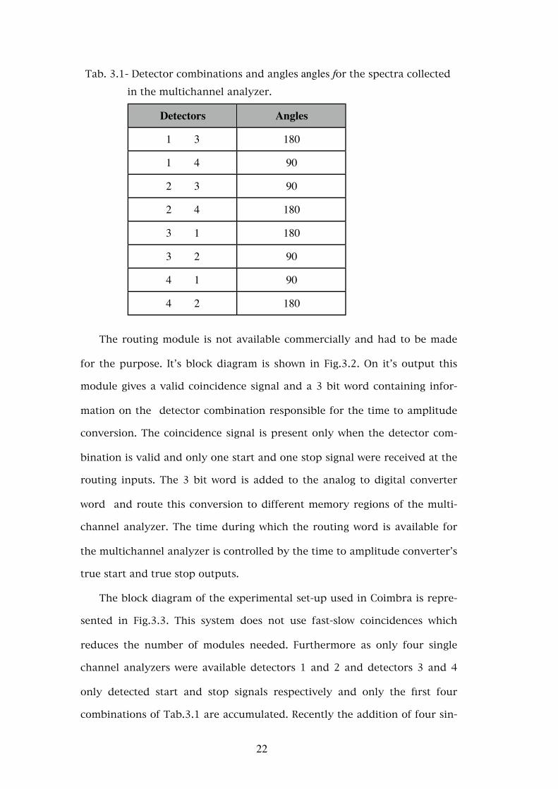
Tab. 3.1- Detector combinations and angles angles for the spectra collected

in the multichannel analyzer.

Detectors Angles

1 3 180

1 4 90

2 3 90

2 4 180

3 1 180

3 2 90

4 1 90

4 2 180

The routing module is not available commercially and had to be made

for the purpose. It’s block diagram is shown in Fig.3.2. On it’s output this

module gives a valid coincidence signal and a 3 bit word containing infor-

mation on the detector combination responsible for the time to amplitude

conversion. The coincidence signal is present only when the detector com-

bination is valid and only one start and one stop signal were received at the

routing inputs. The 3 bit word is added to the analog to digital converter

word and route this conversion to different memory regions of the multi-

channel analyzer. The time during which the routing word is available for

the multichannel analyzer is controlled by the time to amplitude converter’s

true start and true stop outputs.

The block diagram of the experimental set-up used in Coimbra is repre-

sented in Fig.3.3. This system does not use fast-slow coincidences which

reduces the number of modules needed. Furthermore as only four single

channel analyzers were available detectors 1 and 2 and detectors 3 and 4

only detected start and stop signals respectively and only the first four

combinations of Tab.3.1 are accumulated. Recently the addition of four sin-

22

gle channel analyzers made possible the use of all eight spectra combina-

tions.

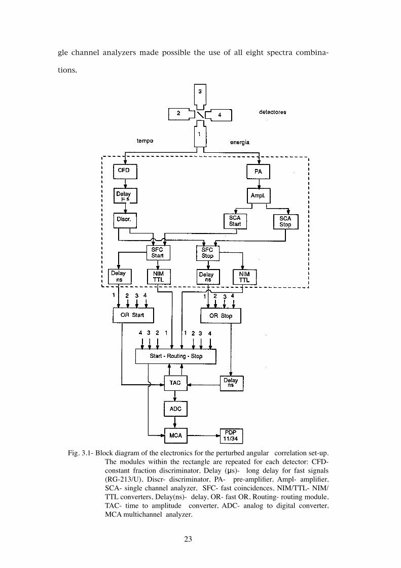
Fig. 3.1- Block diagram of the electronics for the perturbed angular correlation set-up.

The modules within the rectangle are repeated for each detector: CFD- constant fraction discriminator, Delay (μs)- long delay for fast signals (RG-213/U), Discr- discriminator, PA- pre-amplifier, Ampl- amplifier, SCA- single channel analyzer, SFC- fast coincidences, NIM/TTL- NIM/TTL converters, Delay(ns)- delay, OR- fast OR, Routing- routing module, TAC- time to amplitude converter, ADC- analog to digital converter, MCA multichannel analyzer.

23

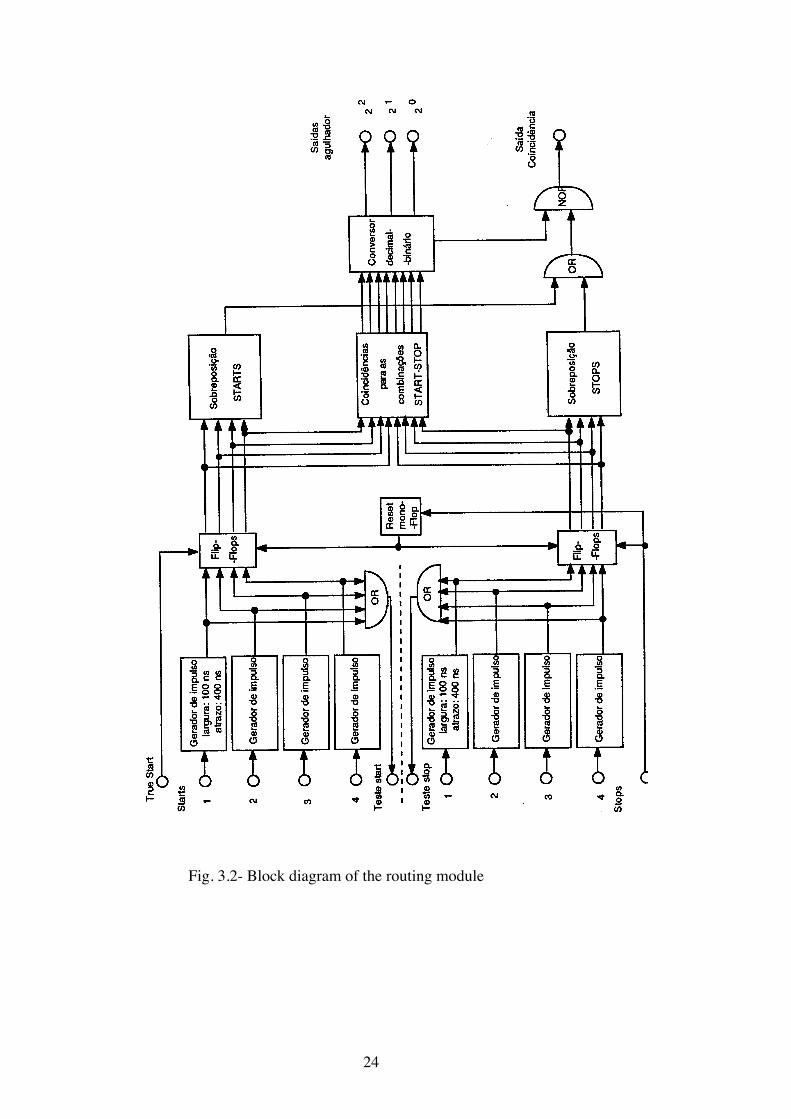
Fig. 3.2- Block diagram of the routing module

24

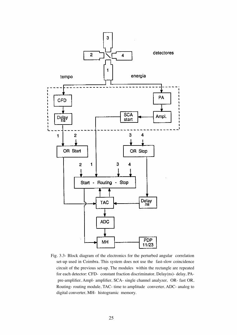
Fig. 3.3- Block diagram of the electronics for the perturbed angular correlation set-up used in Coimbra. This system does not use the fast-slow coincidence circuit of the previous set-up. The modules within the rectangle are repeated for each detector: CFD- constant fraction discriminator, Delay(ns)- delay, PA- pre-amplifier, Ampl- amplifier, SCA- single channel analyzer, OR- fast OR, Routing- routing module, TAC- time to amplitude converter, ADC- analog to digital converter, MH- histogramic memory.

25

The detectors used in this system consist of sodium iodide scintillators cou-

pled to XP-2020 photomultipliers and a time resolution of 2.7ns was

achieved.

Besides the perturbed angular correlation experiments also positron an-

nihilation experiments are performed in Coimbra. Therefore a modular data

acquisition system with independent analog to digital converters was devel-

oped. The acquisition process is controlled by a computer thru an appropri-

ate CAMAC interface. This system is described in Appendix B.

3.1.2 - Cryostat and temperature control

All measurements were made in the temperature range between 8K and

300K. To achieve these temperatures the samples were placed in a closed

cycle helium cryostat. The temperature is controlled by a high precision PID

controller with an uncertainty of ±0.2K. In Fig.3.4 the sample holder is rep-

resented.

b)

3

4

1

2

amostra

Cu

2º estágio do refrigerador

5mm

a)

48mm

32mm

sensor

Fig. 3.4- a) Sample holder for the closed cycle helium cryostat.

b) Relative position of the sample holder and the detectors in order to minimize self-absorption.

26

3.2 Sample preparation

3.2.1 - Probe atom dilution

As was previously refered to perform perturbed angular correlation ex-

periments in metals it’s necessary to dilute the radioactive probe in the

metal studied. In metals this dilution depends on the metal affinity to form

alloys with the radioactive species.

In the present work 181Hf was used as radioactive probe as it presents

several advantages for these studies: Hafnium is soluble in metals of the va-

nadium group [Moffat 78] and since it occupies substitutional places in the

cubic lattice the electric field gradient is zero in the absence of other de-

fects; on the other hand the fact that the recoil energy of the β decay of

181Hf to 181Ta (approximately 2eV) is much smaller than the average en-

ergy necessary to move a lattice atom to an interstitial position (typically

25eV [Nelson 75]) the radioactive 181Ta remains in the same position as it’s

parent nucleus. When studying tantalum, hafnium has also the advantage of

being transformed into a lattice atom by the decay leaving the lattice unper-

turbed. The half-life of 181Hf is 42.4 days which allows several months for

measurements. Also the activated 181Hf is very easy to obtain by irradiating

in a reactor natural hafnium according to the reaction 180Hf(n,γ) 181Hf.

The hafnium for irradiation (approximately 1mg) is encapsulated in a

quartz ampoule to facilitate transport and irradiation. The activation was

done at the Kernforschungsanlage Jülich with a thermal neutron flux of

1015 n/cm2s during approximately two months and the specific activity

reached was of the order of 200mCi/mg. One disadvantage of this nuclide

is the fact that the irradiated hafnium is still essentially inactive (for the

27

specific activities reached only 10% of the atoms are activated) and as, in

general it is not possible to separate the activated atoms we must dilute a

high fraction of inactive hafnium in the metal.

The dilution of the radioactive species in the metal may be performed

by either of the three following methods: diffusion, implantation or melting

of the two metals. As the diffusion coefficients of hafnium in tantalum and

niobium are very small the diffusion method can not be used. Implantation

raises some technical problems specially the strong and persistent contami-

nations of the accelerator due to the long half-life of 181Hf. The samples

were therefore prepared by melting together tantalum and niobium of

99.96% purity, both from Materials Research Corporation, and irradiated

hafnium (96.6% Hf, 3.3% Zr). Melting was performed in an electron

gun in ultra-high vacuum

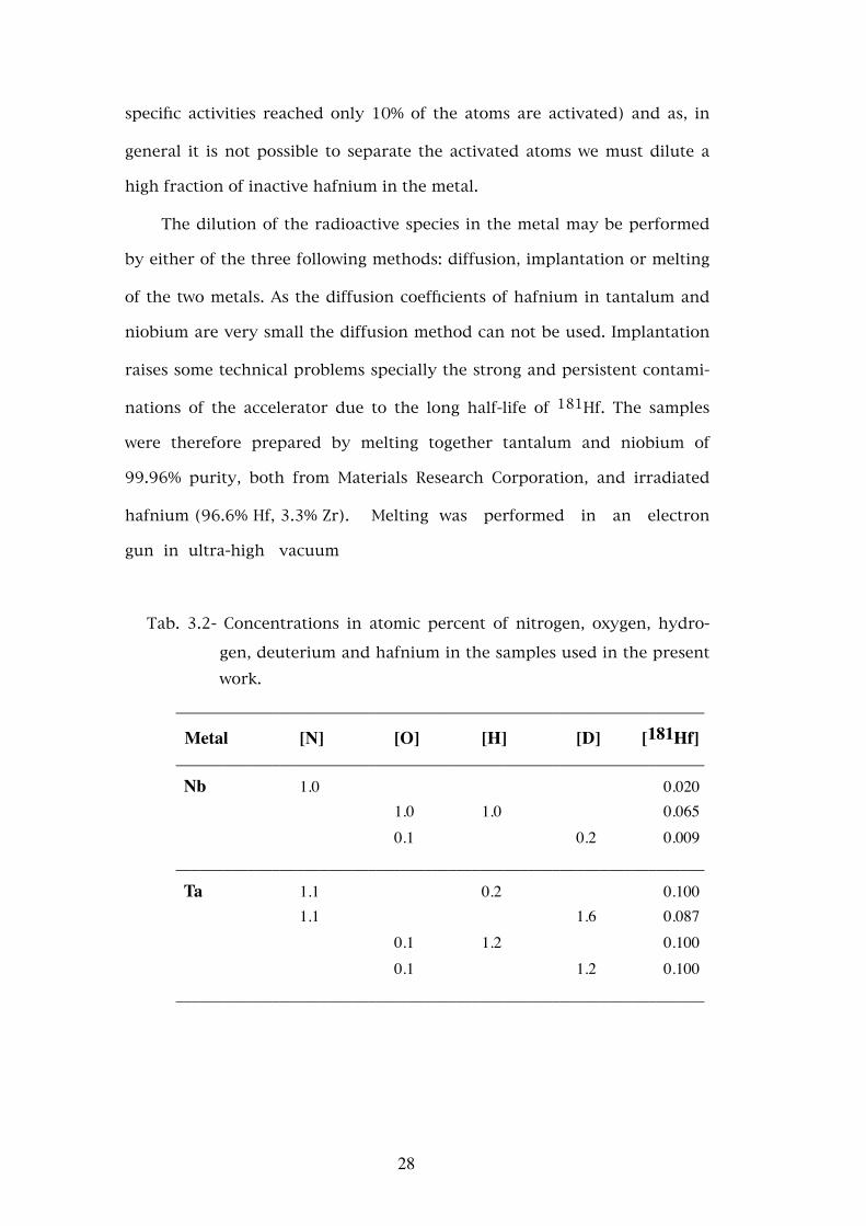
Tab. 3.2- Concentrations in atomic percent of nitrogen, oxygen, hydro-

gen, deuterium and hafnium in the samples used in the present work.

__________________________________________________________________

Metal [N] [O] [H] [D] [181Hf]__________________________________________________________________ Nb 1.0 0.020 1.0 1.0 0.065 0.1 0.2 0.009__________________________________________________________________ Ta 1.1 0.2 0.100 1.1 1.6 0.087 0.1 1.2 0.100 0.1 1.2 0.100__________________________________________________________________

28

NbHf181

Hf181 Ta

0 10 20 30 40 50 60

tempo (ns)

0.0

-0.1

-0.2

0.0

-0.3

-0.2

-0.1

R (t)

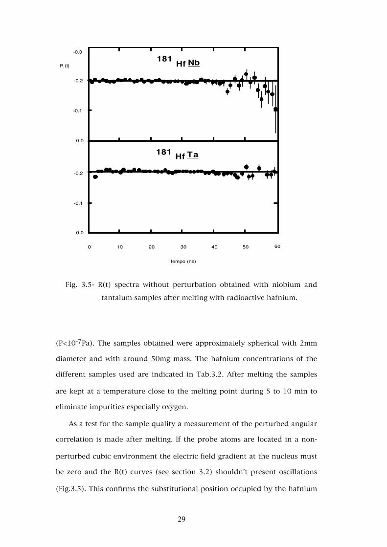
Fig. 3.5- R(t) spectra without perturbation obtained with niobium and

tantalum samples after melting with radioactive hafnium.

(P<10-7Pa). The samples obtained were approximately spherical with 2mm

diameter and with around 50mg mass. The hafnium concentrations of the

different samples used are indicated in Tab.3.2. After melting the samples

are kept at a temperature close to the melting point during 5 to 10 min to

eliminate impurities especially oxygen.

As a test for the sample quality a measurement of the perturbed angular

correlation is made after melting. If the probe atoms are located in a non-

perturbed cubic environment the electric field gradient at the nucleus must

be zero and the R(t) curves (see section 3.2) shouldn’t present oscillations

(Fig.3.5). This confirms the substitutional position occupied by the hafnium

29

atoms, the absence of impurities after melting and also shows that the num-

ber of hafnium atoms in non-cubic environments, such as grain boundaries,

is not detectable.

3.2.2 - Nitrogen and oxygen dilution

The dilution of nitrogen or oxygen in the samples is made from the gas

phase. Before loading with any of these gases the superficial oxide layer is

removed by heating as described before. The pressures and temperatures

used are taken from the solubility data for these metals available in the

literature [Taylor 67, Smithels 67 e Schulze 77,79]. In the case of tantalum

the dilution of oxygen was performed at a temperature of 2300K and a par-

tial pressure of oxygen of 3x10-4Pa and for nitrogen 2020K and 0.1Pa were

used. For niobium the temperatures and pressures used were 2400K and

0.01Pa (or 0.001Pa) for oxygen and 2300K and 0.5Pa for nitrogen.

Special care must be taken to dilute nitrogen in these metals to avoid

contamination in particular from oxygen. Indeed the solubility of nitrogen

in these metals is much smaller than that of oxygen and oxygen also diffuses

faster than nitrogen [Fromm80]. For this reason the initial vacuum before

loading was better than 5x10-8Pa and high purity nitrogen (99.999%)

flowed through an adsorbing coal filter in order to eliminate any oxygen

impurity. The nitrogen and oxygen concentrations of the samples used are

indicated in Tab.3.2.

30

3.2.3 - Hydrogen and deuterium dilution

Implantation could not be used to dilute hydrogen or deuterium due to

the small dimensions of the samples and to the fact that the energies avail-

able were too high and would cause unwanted defects during implantation.

Dilution from the gas phase was also not used since at the temperatures at

which the samples must be heated (of the order of 400°C to 500°C for low

concentrations of the order of 1%[Fromm 80]) oxygen from the surface ox-

ide layer diffuses and is captured by hafnium.

The method used was electrolysis in a solution of H2SO4 1 molar (for

deuterium D2SO4 in D2O was used). The sample is placed in a gold gasket

which also makes the electric contact with the rest of the circuit. The elec-

trolytic solution is kept at 80°C for tantalum and 90°C for niobium. At lower

temperatures ordered phases of the metal-hydrogen system are formed

during electrolysis which may produce small cracks in the sample prevent-

ing the control of the hydrogen quantity dissolved. As for deuterium the

surface potential barrier is larger than for hydrogen the surface oxide layer

is removed before electrolysis. For this purpose the samples are kept for 10

to 15 seconds in an etching solution made from 1ml HNO3 + 2.5ml of H2SO4

(for deuterium D2O and D2SO4 are used) to which 1ml of HF is added im-

mediately before using.

3.2.4 - Hydrogen and deuterium concentration determination

In the electrolysis the concentrations of hydrogen (deuterium) is condi-

tioned by parameters such as the current used, the geometrical shape of the

sample, time, temperature, etc. For low concentrations it is possible to pre-

31

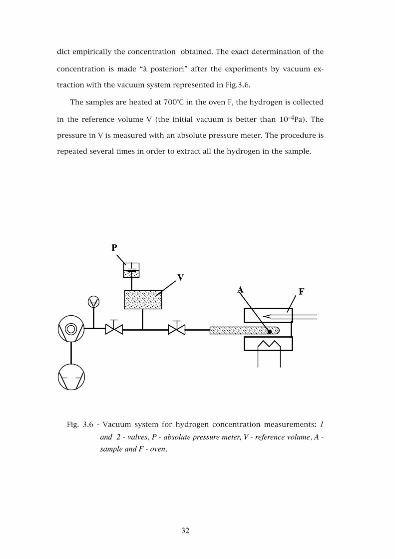
dict empirically the concentration obtained. The exact determination of the

concentration is made “à posteriori” after the experiments by vacuum ex-

traction with the vacuum system represented in Fig.3.6.

The samples are heated at 700°C in the oven F, the hydrogen is collected

in the reference volume V (the initial vacuum is better than 10-4Pa). The

pressure in V is measured with an absolute pressure meter. The procedure is

repeated several times in order to extract all the hydrogen in the sample.

A

P

VF

Fig. 3.6 - Vacuum system for hydrogen concentration measurements: 1 and 2 - valves, P - absolute pressure meter, V - reference volume, A - sample and F - oven.

32

3.3 - Data analysis

As we refered in chapter 2 in perturbed angular correlation experiments

the function W(θ,t) contains all the information regarding the hyperfine in-

teraction. This function may be obtained experimentally by a convenient

analysis of the time spectra. This analysis eliminates the exponential decay

and minimizes the effects due to detectors efficiencies, self-absorption in the

samples, width and live time of the time analyzer channels, finite time

resolution and background coincidences. The most commonly used method

for these corrections is based on the use of four detectors and the storage

of the different time spectra which are then added in a convenient way as

described below.

3.3.1 - The perturbation factor extracted from the time spectra

The coincidence count rate between two detectors i and j, whose axis

form an angle θ with a radioactive sample at the vertex is given by

Cij(θ,t) = N0 Pij(θ,t) Tij(t) Lij(t) + Bij(θ,t) (3.1)

where t is the time interval between the detection of γ1 and γ2, N0 is the

number of cascades per unit time occurring in the sample, Pij(θ,t) is the

probability of detecting γ1 and γ2 at an angle θ with a time difference t,

Tij(t) is the live time, Lij(t) is the channel width of the time analyzer and

Bij(θ,t) is the background coincidences count rate.

33

If we consider a detection system in which the angle θ is defined by two

point detectors and the time interval is measured with infinite precision

then the probability Pij, for t>0, is given by:

Pij (θ, t) = ------1τN

ei ej ai j e-t/τ

Ν W (θ, t) (3.2)

where τN is the lifetime of the intermediate state, ei and ej are the detector

efficiencies of the detectors for the energies of γ1 and γ2, aij is a correction

factor due to the source self-absorption and W(θ,t) is the correlation func-

tion of the γ cascade. However the time resolution and the solid angle de-

fined by the detectors are finite and the probability Pij must be corrected

accordingly. For t>Γt (Γt is the half maximum width of the time resolution

function of the experimental system) the effect of the finite time resolution

may be written as an attenuation factor, frequency dependent, which affects

the modulation amplitudes of W(θ,t) [Pleiter 73]. For cylindrical detectors

with their axes oriented towards the source the effect of finite solid angle is

described by an attenuation factor of each term of W(θ,t) and which are

tabulated [Yates 65]. The correction due to the finite time resolution used is

described in section 3.3.2 and no correction due to the finite solid angle was

considered as the fits were always normalized to the anisotropy coefficient

sk0 observed experimentally.

The first step in the manipulation of the experimental data is the sub-

traction of the background coincidences count rate. The most direct method

is to calculate this count rate in a zone of the time spectra where the first

term of (3.1) is zero. This occurs for t<0 or t >> τN. The live time Tij(t) may

influence the background and for high count rates Tij(t) may vary strongly

with t. Therefore it is important to subtract correctly the background count

34

rate since a difference of a few percent in this value may lead to distortions

of W(θ,t) which may be interpreted as hyperfine interactions [Arends 80].

To minimize the effects of Tij(t) low count rates were used and as a suffi-

cient number of channels were available in the multichannel analyzer the

background count rate for t>0 was always calculated from channels in the

region t>>τN. With the count rates and counting times used after 5 or 6 τN

periods there was no appreciable contribution from the decay of the inter-

mediate state.

The count rate corrected for the background C+ij(θ,t) is given by:

C+ij (θ, t) = Ci j (θ, t) - Bi j (θ, t) = N0 ------

1τN

Ei j (t) e-t/τ

Ν W (θ, t) (3.3)

where Eij(t) = ei ej aij Tij(t) Lij(t).

After this operation the zeros of the several spectra must be made to

coincide. This is required in order to be able to use the channels for times

t<τN [Arends 80]. the time t=0 is ideally defined by the centroid of the

prompt curve obtained with radiation of the same energies of the γ rays of

the cascade. As usually there are no prompt cascades available with the

required energies the positron annihilation radiation (obtained for instance

from the decay of 22Na) or the prompt cascade of 60Co are used. However

in our case the time zero of each spectra were always adjusted before each

measurement so that the difference between them is smaller than one or

two channels, and therefore the prompt curve was not measured. As long as

the difference between the time zero of the several spectra is smaller than

the time resolution of the experimental system the misalignment only af-

fects the channels for t<τN. Furthermore this effect is partially canceled in

the data analysis programme where a first approximation for the time zero

35

of each spectrum is determined and all spectra are aligned by the same time

zero.

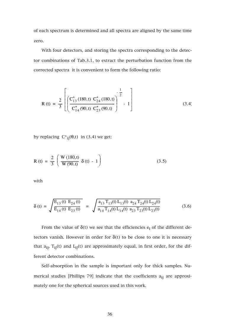
With four detectors, and storing the spectra corresponding to the detec-

tor combinations of Tab.3.1, to extract the perturbation function from the

corrected spectra it is convenient to form the following ratio:

R (t) = ------23

⎢⎢⎢⎢

⎡

⎣

⎥⎥⎥⎥

⎤

⎦⎜⎜⎛

⎝⎟⎟⎞

⎠---------------------------------------------------------C+

13 (180, t) C+24 (180, t)

C+14 (90, t) C+

23 (90, t)

- -------12

- 1 (3.4)

by replacing C+ij(θ,t) in (3.4) we get:

R (t) = ------23 ⎜

⎛⎝ ⎟

⎞⎠ -----------------------

W (180, t)W (90, t) δ (t) - 1 (3.5)

with

δ (t) = ----------------------------------E13 (t) E24 (t)E14 (t) E23 (t) = ---------------------------------------------------------------------------------

a13 T13(t) L13(t) a24 T24(t) L24(t)a14 T14(t) L14(t) a23 T23(t) L23(t) (3.6)

From the value of δ(t) we see that the efficiencies ei of the different de-

tectors vanish. However in order for δ(t) to be close to one it is necessary

that aij, Tij(t) and Lij(t) are approximately equal, in first order, for the dif-

ferent detector combinations.

Self-absorption in the sample is important only for thick samples. Nu-

merical studies [Phillips 79] indicate that the coefficients aij are approxi-

mately one for the spherical sources used in this work.

36

Lij(t) and Tij(t) depend mainly on the electronic system used and on the

experimental conditions of the measurements. As their dependence on the

delay time t is usually small they are considered to be approximately con-

stant. They may however affect considerably the results if there is a high

differential or integral non-linearity of the time to amplitude converter or of

the multichannel analyzer. The influence of the experimental conditions

was minimized in this work using symmetric geometries, low count rates

and similar coincidence count rates in the various detector combinations.

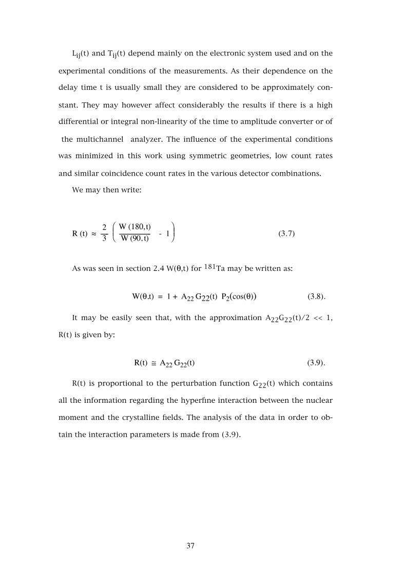
We may then write:

R (t) ≈ ------23 ⎜

⎛⎝ ⎟

⎞⎠ -----------------------

W (180, t)W (90, t) - 1 (3.7)

As was seen in section 2.4 W(θ,t) for 181Ta may be written as:

W(θ,t) = 1 + A22 G22(t) P2(cos(θ)) (3.8).

It may be easily seen that, with the approximation A22G22(t)/2 << 1,

R(t) is given by:

R(t) ≅ A22 G22(t) (3.9).

R(t) is proportional to the perturbation function G22(t) which contains

all the information regarding the hyperfine interaction between the nuclear

moment and the crystalline fields. The analysis of the data in order to ob-

tain the interaction parameters is made from (3.9).

37

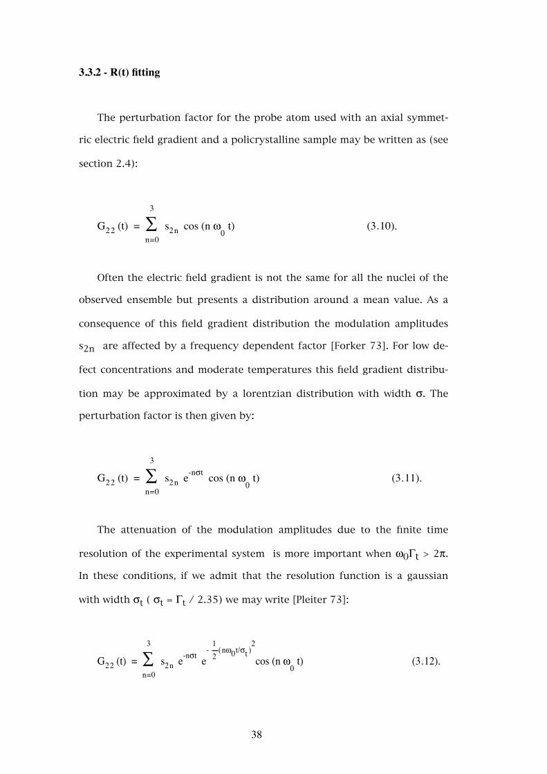
3.3.2 - R(t) fitting

The perturbation factor for the probe atom used with an axial symmet-

ric electric field gradient and a policrystalline sample may be written as (see

section 2.4):

G22 (t) = ∑n=0

3

s2n cos (n ω0 t) (3.10).

Often the electric field gradient is not the same for all the nuclei of the

observed ensemble but presents a distribution around a mean value. As a

consequence of this field gradient distribution the modulation amplitudes

s2n are affected by a frequency dependent factor [Forker 73]. For low de-

fect concentrations and moderate temperatures this field gradient distribu-

tion may be approximated by a lorentzian distribution with width σ. The

perturbation factor is then given by:

G22 (t) = ∑n=0

3

s2n e-nσt cos (n ω0 t) (3.11).

The attenuation of the modulation amplitudes due to the finite time

resolution of the experimental system is more important when ω0Γt > 2π.

In these conditions, if we admit that the resolution function is a gaussian

with width σt ( σt = Γt / 2.35) we may write [Pleiter 73]:

G22 (t) = ∑n=0

3

s2n e-nσt e- -------

12( )nω0t/σt

2

cos (n ω0 t) (3.12).

38

When in the same sample there are k different electric field gradients

the perturbation factor may be written as follows:

G22 (t) = f0 ∑n=0

3

s2n e-nσ0t

+ ∑i=1

k

fi ∑n=0

3

s2n e-nσit e

- -------12( )nω0it/σt

2

cos (n ω0i t) (3.13)

where fi (i=1,...,k) are the fractions of probe atoms perturbed by the electric

field gradient i and f0 is the fraction of probe atoms unperturbed or per-

turbed by a distribution of electric field gradients close to zero.

In the general case of field gradients without axial symmetry (η≠0) the

amplitudes s2n are functions of η and the transition frequencies are no

longer integer multiples of the lowest frequency ω0. The perturbation fac-

tor is then given by:

G22 (t) = f0 ∑n=0

3

s2n e-nσ0t

+ ∑i=1

k

fi ∑n=0

3

s2n(ηi) e-nn(ηi)σit e

- -------12( )nn(ηi)ω0it/σt

2

cos (nn(ηi) ω0i t)

(3.14)

with s2n(η) and nn(η) (nn(η=0)=n) different for each interaction and func-

tions of η. The experimental curve R(t) is adjusted to the function A22G22(t)

with G22(t) given by (3.14) by the least squares method using a gradient

algorithm [Bevington 69]. The adjustable parameters for each interaction

are : the fraction of atoms influenced by the interaction fi, the frequency ω0i

(proportional to the electric field gradient), and the width of the electric

field gradient distribution σi around ω0i. The statistical error is calculated

according to the theory of the propagation of errors for this algorithm

[Bevington 69]. In the analysis programme used the fit of the parameter η is

not included. The values presented for this parameter were obtained calcu-

lating the minimum of χ2 by varying systematically the value of η. The error

39

in η was calculated by the usual approximation of the quadratic variation

of χ2 with η around the minimum [Bevington 69].

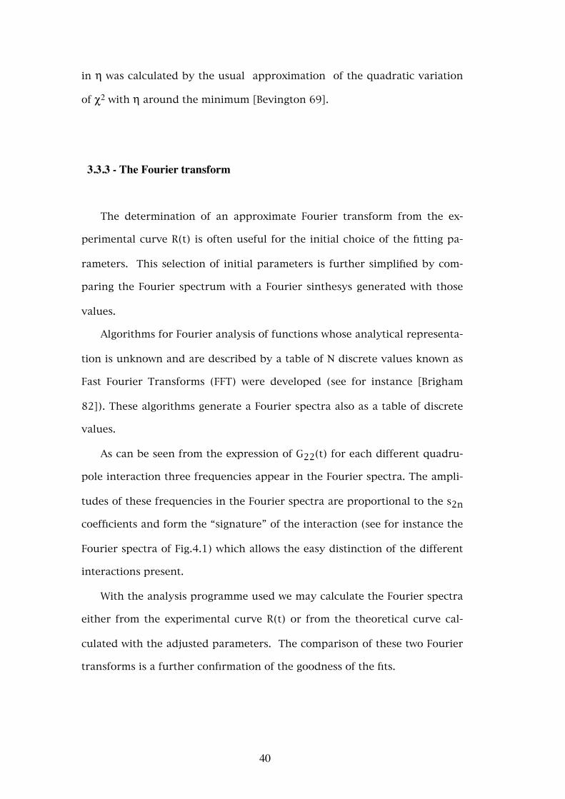
3.3.3 - The Fourier transform

The determination of an approximate Fourier transform from the ex-

perimental curve R(t) is often useful for the initial choice of the fitting pa-

rameters. This selection of initial parameters is further simplified by com-

paring the Fourier spectrum with a Fourier sinthesys generated with those

values.

Algorithms for Fourier analysis of functions whose analytical representa-

tion is unknown and are described by a table of N discrete values known as

Fast Fourier Transforms (FFT) were developed (see for instance [Brigham

82]). These algorithms generate a Fourier spectra also as a table of discrete

values.

As can be seen from the expression of G22(t) for each different quadru-

pole interaction three frequencies appear in the Fourier spectra. The ampli-

tudes of these frequencies in the Fourier spectra are proportional to the s2n

coefficients and form the “signature” of the interaction (see for instance the

Fourier spectra of Fig.4.1) which allows the easy distinction of the different

interactions present.

With the analysis programme used we may calculate the Fourier spectra

either from the experimental curve R(t) or from the theoretical curve cal-

culated with the adjusted parameters. The comparison of these two Fourier

transforms is a further confirmation of the goodness of the fits.

40

CHAPTER 4

OXYGEN AND NITROGEN STUDIES

IN TANTALUM AND NIOBIUM

As oxygen and nitrogen present a high solubility in the metals of the Vb

group of the periodic table, vanadium, niobium and tantalum, studies with

high concentrations of these elements may be performed without perturba-

tions due to precipitates. However internal friction studies in these systems

suggest the formation of On complexes in these metals due to precipitation

for concentrations as low as 1 at.% [Cost 84]. On the other hand results in

high purity systems suggest a repulsive interaction between oxygen atoms

[Weller 85b] which should inhibit the formation of the complexes suggested

by Cost. A similar behaviour should be observed for nitrogen. Weller and

Giballa [Weller 85a, Gibala 85] suggest that the complexes observed are due

to the interaction of oxygen with nitrogen which exists as an impurity in the

samples. Inelastic X-Ray studies [Schubert 84, Dosch 85] confirm the non-

existence of nitrogen precipitates in niobium.

4.1 - Experimental results

The study of the quadrupole interaction due to hydrogen (deuterium)

trapped at oxygen (nitrogen) requires a previous knowledge of the interac-

41

tions due to oxygen and nitrogen alone as well as the temperature depend-

ence of the parameters characterizing these interactions. These experiments

were done with the samples indicated in Tab.3.2 before loading with hydro-

gen or deuterium. The samples were placed in a closed cycle helium criostat

and the system described in section 3.1 was used for the measurements.

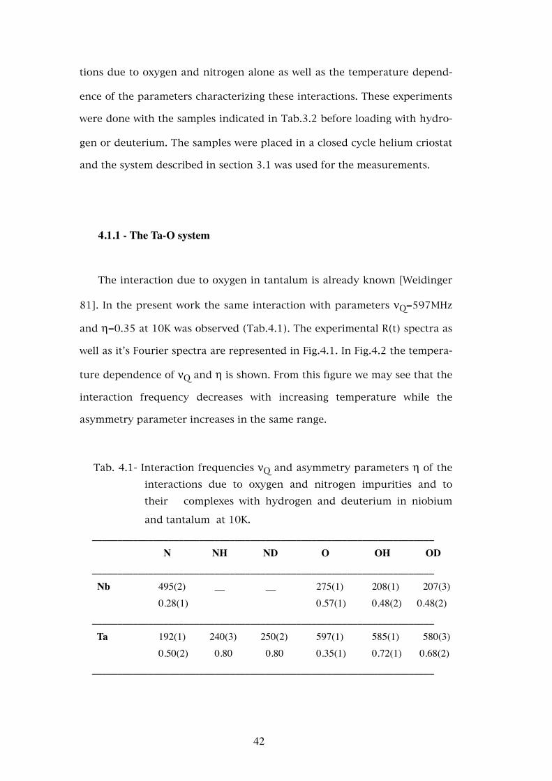
4.1.1 - The Ta-O system

The interaction due to oxygen in tantalum is already known [Weidinger

81]. In the present work the same interaction with parameters νQ=597MHz

and η=0.35 at 10K was observed (Tab.4.1). The experimental R(t) spectra as

well as it’s Fourier spectra are represented in Fig.4.1. In Fig.4.2 the tempera-

ture dependence of νQ and η is shown. From this figure we may see that the

interaction frequency decreases with increasing temperature while the

asymmetry parameter increases in the same range.

Tab. 4.1- Interaction frequencies νQ and asymmetry parameters η of the interactions due to oxygen and nitrogen impurities and to their complexes with hydrogen and deuterium in niobium

and tantalum at 10K.___________________________________________________________________ N NH ND O OH OD___________________________________________________________________ Nb 495(2) __ __ 275(1) 208(1) 207(3) 0.28(1) 0.57(1) 0.48(2) 0.48(2)___________________________________________________________________ Ta 192(1) 240(3) 250(2) 597(1) 585(1) 580(3) 0.50(2) 0.80 0.80 0.35(1) 0.72(1) 0.68(2)___________________________________________________________________

42

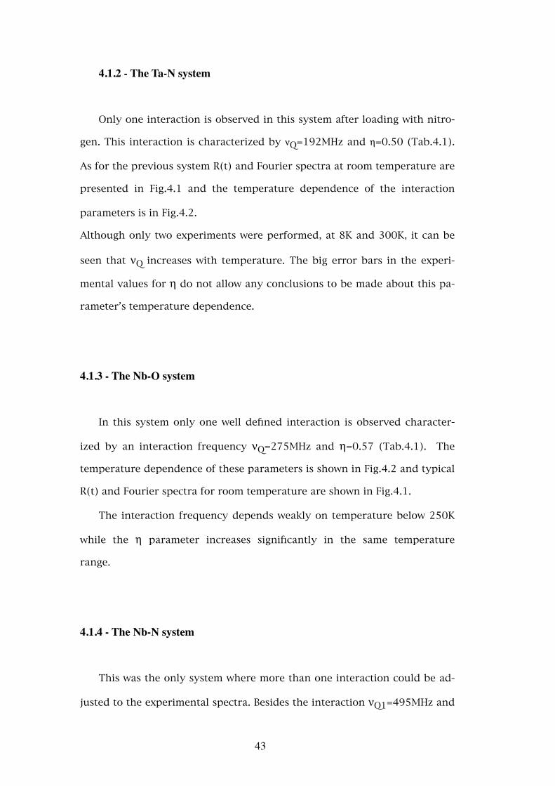
4.1.2 - The Ta-N system

Only one interaction is observed in this system after loading with nitro-

gen. This interaction is characterized by νQ=192MHz and η=0.50 (Tab.4.1).

As for the previous system R(t) and Fourier spectra at room temperature are

presented in Fig.4.1 and the temperature dependence of the interaction

parameters is in Fig.4.2.

Although only two experiments were performed, at 8K and 300K, it can be

seen that νQ increases with temperature. The big error bars in the experi-

mental values for η do not allow any conclusions to be made about this pa-

rameter’s temperature dependence.

4.1.3 - The Nb-O system

In this system only one well defined interaction is observed character-

ized by an interaction frequency νQ=275MHz and η=0.57 (Tab.4.1). The

temperature dependence of these parameters is shown in Fig.4.2 and typical

R(t) and Fourier spectra for room temperature are shown in Fig.4.1.

The interaction frequency depends weakly on temperature below 250K

while the η parameter increases significantly in the same temperature

range.

4.1.4 - The Nb-N system

This was the only system where more than one interaction could be ad-

justed to the experimental spectra. Besides the interaction νQ1=495MHz and

43

η1=0.28 presented in Tab.4.1, two other interactions with smaller fractions

are observed characterized by νQ2=240MHz and η2=0.68 and νQ3=350MHz

and η3=0.73. The R(t) and Fourier spectra are shown in Fig.4.1. The interac-

tion νQ1 indicated by the lines in the Fourier spectrum is clearly dominant

over the other two. In two different samples which were loaded with nitro-

gen in the same conditions and with similar concentrations (see Tab.3.2) it

was observed that in each sample the fraction of probe atoms perturbed by

νQ2 and νQ3 is smaller than the fraction of νQ1 and the ratio of these three

fractions is constant with temperature. However this ratio depends on the

sample considered. The ratio (f1: f2: f3) of the observed fractions was (1 :

0.6 : 0.3) and (1 : 0.3 : 0.5) for the two samples studied. On the other hand

while νQ1 and η1 are identical between the two samples νQ2, η2 and νQ3, η3

vary by approximately 16% in the same samples. Within the experimental

uncertainty no significant variation of these parameters with temperature

was observed.

These facts lead to the conclusion that the interactions νQ2 and νQ3

must be due to a mixture of different complexes, which are stable in the

temperature range studied, and that the number of these defects depend

strongly on the conditions in which samples are prepared. The well defined

and sample independent interaction νQ1 must be due to the interaction of

one single nitrogen atom with the hafnium probe.

The temperature dependence of νQ1 and η1 is shown in Fig.4.2. We may

see from this figure that νQ1 is almost constant while η1 is constant up to

150K and then increases slightly.

44

a) b)

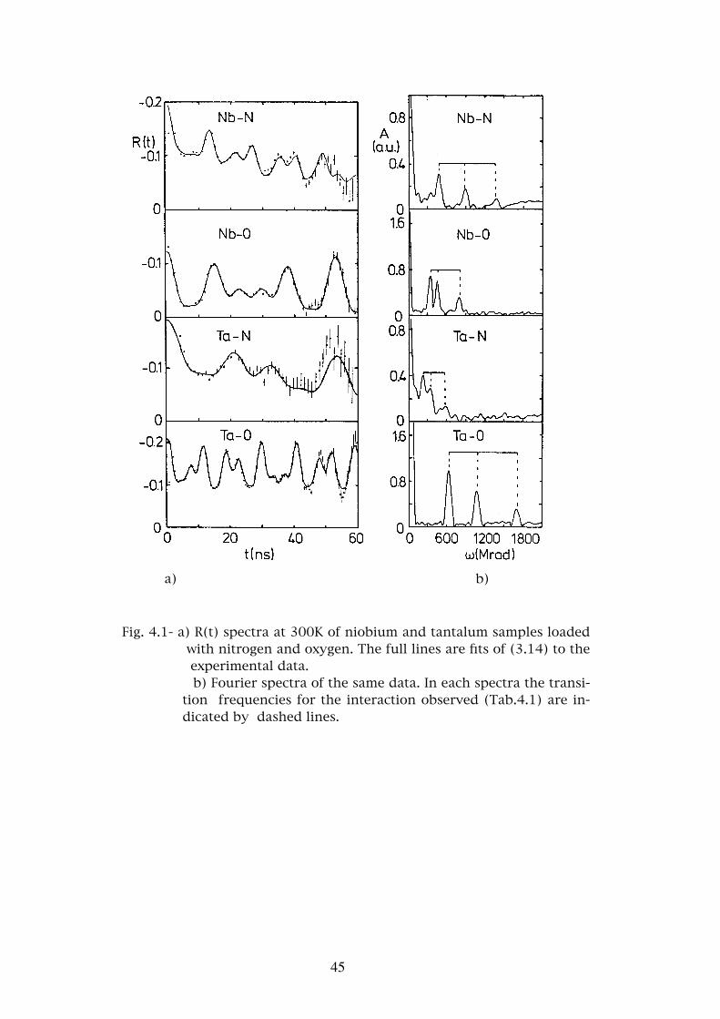
Fig. 4.1- a) R(t) spectra at 300K of niobium and tantalum samples loaded with nitrogen and oxygen. The full lines are fits of (3.14) to the experimental data.

b) Fourier spectra of the same data. In each spectra the transi-tion frequencies for the interaction observed (Tab.4.1) are in-dicated by dashed lines.

45

a) b)

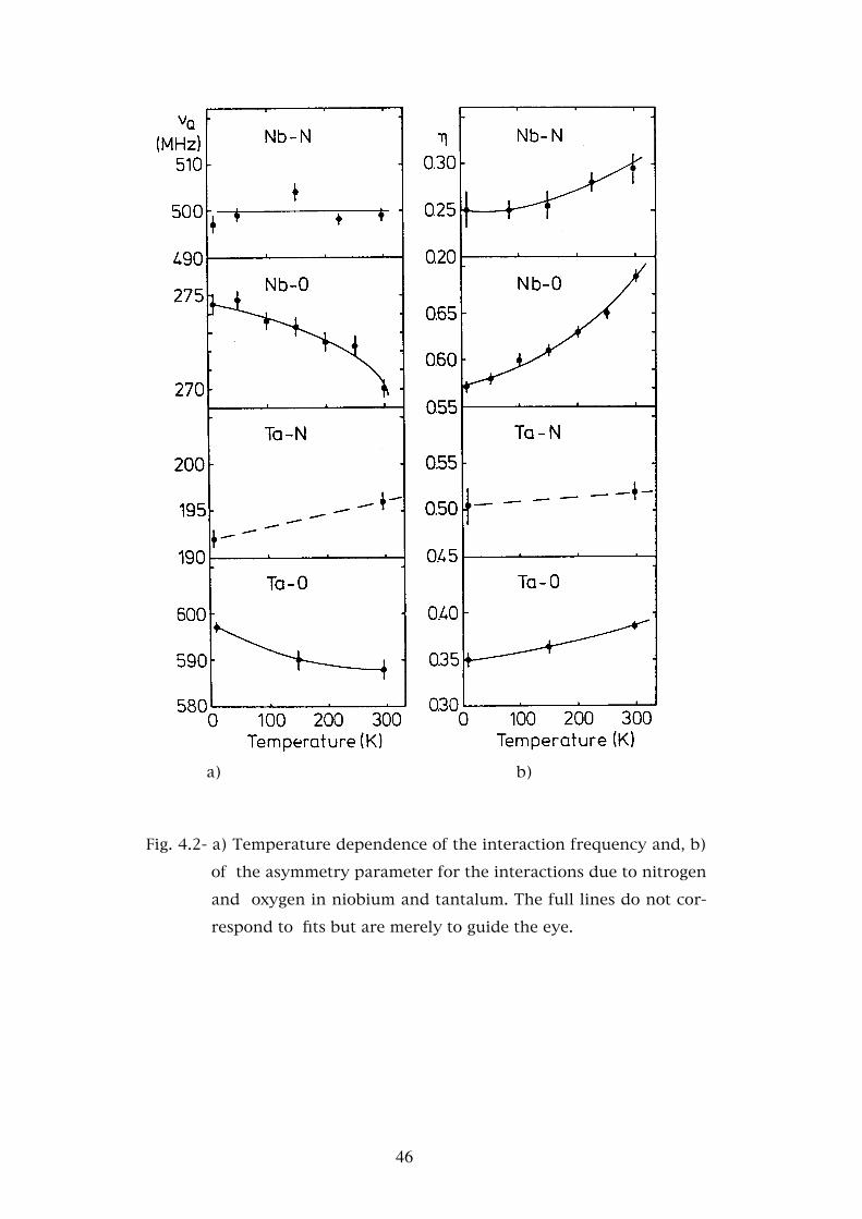
Fig. 4.2- a) Temperature dependence of the interaction frequency and, b)

of the asymmetry parameter for the interactions due to nitrogen

and oxygen in niobium and tantalum. The full lines do not cor-

respond to fits but are merely to guide the eye.

46

4.2 - Discussion

In order to understand the relative values of the interaction parameters

for the different systems, information about the position of the probe atom

relative to the interstitial impurity is required. The position occupied by

oxygen and nitrogen in the metallic lattices of niobium, tantalum and vana-

dium has been determined by ion channeling experiments [Hiraga 77,

Takahashi 78, Kaim 79, Carstanjen 82, Shakun 85] which have shown that

both oxygen and nitrogen occupy interstitial octahedral positions in these

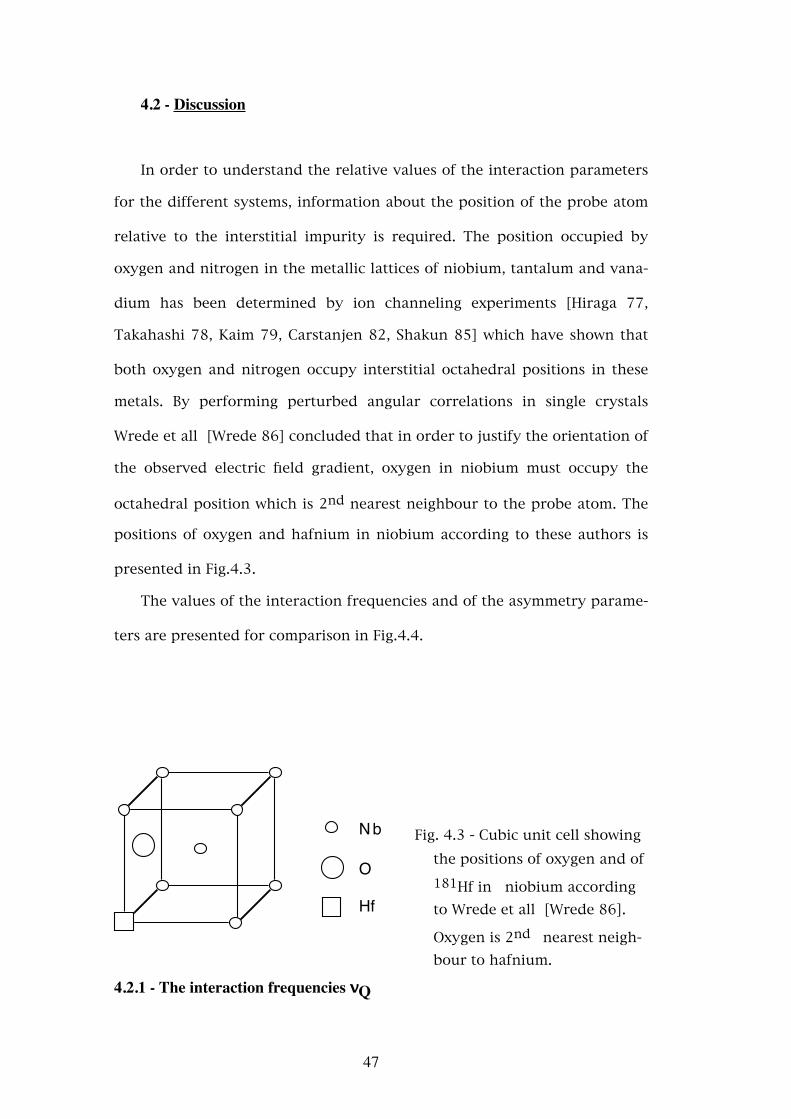
metals. By performing perturbed angular correlations in single crystals

Wrede et all [Wrede 86] concluded that in order to justify the orientation of

the observed electric field gradient, oxygen in niobium must occupy the

octahedral position which is 2nd nearest neighbour to the probe atom. The

positions of oxygen and hafnium in niobium according to these authors is

presented in Fig.4.3.

The values of the interaction frequencies and of the asymmetry parame-

ters are presented for comparison in Fig.4.4.

Fig. 4.3 - Cubic unit cell showing the positions of oxygen and of 181Hf in niobium according to Wrede et all [Wrede 86].

Oxygen is 2nd nearest neigh-bour to hafnium.

4.2.1 - The interaction frequencies νQ

Nb

O

Hf

47

Due to their low diffusion coefficient in the temperature range studied

oxygen and nitrogen when captured by hafnium remain immobile in their

interstitial positions after the decay of the probe atom. On the other hand as

the first excited state of the 181Ta cascade has a lifetime of 25.7µs (Fig.2.3)

and as the electronic relaxation times in metals are of the order of picosec-

onds and the lattice ion relaxation times are of the order of nano-seconds,

when the angular correlation is observed there is no longer any influence of

the original charge distribution due to the probe atom 181Hf. Therefore we

may consider that the system studied consists of the metallic lattice, the

radioactive atom 181Ta and the oxygen or nitrogen impurity.

If the positions of oxygen and nitrogen relative to the radioactive atom

are the same, the variation of the interaction frequencies must be essentially

due to differences of the electronic charge distribution caused by the differ-

ent valence of oxygen and nitrogen and, in the case of niobium, also due to

the radioactive atom which is an impurity in this metal.

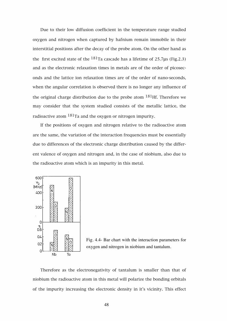
Fig. 4.4- Bar chart with the interaction parameters for oxygen and nitrogen in niobium and tantalum.

Therefore as the electronegativity of tantalum is smaller than that of

niobium the radioactive atom in this metal will polarize the bonding orbitals

of the impurity increasing the electronic density in it’s vicinity. This effect

48

will be stronger for nitrogen since this atom may receive up to three elec-

trons in it’s valence shell as opposed to two in oxygen. For this reason we

expect that the interaction frequency due to nitrogen is larger than that due

to oxygen in this metal, νQN > νQO, and that is what was experimentally

observed (see Fig.4.4).

In tantalum the charges involved are the same but as the radioactive

atom is the same as the lattice atoms, this charge will be equally distributed

by all the nearest neighbours of the interstitial impurity. As the bonding

orbitals of oxygen and nitrogen are p orbitals the distribution of charge is

larger for nitrogen, since it may receive three electrons which are then dis-

tributed by it’s 6 nearest neighbours, than for oxygen where the electrons

received form bonds to the four 2nd nearest neighbours avoiding the high

electronic density of the 1st nearest neighbour tantalum atoms. Therefore in

spite of nitrogen attracting more electrons we expect oxygen to give rise to a

higher interaction frequency, νQN < νQO as was experimentally observed

(see Fig.4.4).

The observation of more than one interaction frequency in the Nb-N

system shows, as was already mentioned, that several types of defects with

different numbers of nitrogen atoms are captured by the hafnium probe.

The formation of these precipitates seem to be strongly dependent on the

sample preparation particularly the cooling procedure. Cooling of samples

by flowing cool helium into the vacuum chamber immediately after switch-

ing the heating current off has been successfully used to quench the high

temperature α phase random distribution of nitrogen atoms in niobium and

no precipitates have been observed [Rowe 80, Schubert 84]. The samples

used in the present work were cooled simply by switching the electron gun

current off. The electron gun is enclosed in a glass enclosure with only one

open end in order to prevent the radioactive contamination of the vacuum

49

chamber. This difficults the gas flow around the sample and we should ex-

pect to have low cooling rates in this conditions. In the samples studied an

equal number of probe atoms with only one nitrogen and with more than

one nitrogen atom in it’s vicinity are observed which indicates that the

number of nitrogen atoms in precipitates is high. This indicates that substi-

tutional hafnium is an efficient trapping center for nitrogen as, according to

the phase-diagram for this system, at room temperature and for 1 at.% ni-

trogen in niobium only approximately 5% of the nitrogen atoms precipitate.

With the results available the identification of the complexes causing the

two extra interactions is not possible.

4.2.2 - The asymmetry parameters η

An increase of the asymmetry parameter when the temperature is in-

creased from 10K to 300K is observed for all systems. The relative variation

of this parameter is larger for niobium than for tantalum, while in tantalum

this variation is smaller than 10% in niobium is approximately 20% in the

same temperature range. This larger variation of η in niobium may be due

to an additional distortion of the electronic charge distribution due to the

fact that the radioactive atom (181Ta) is an impurity in this lattice.

From the definition of the asymmetry parameter, η =(Vyy- Vxx )/Vzz, we

may see that a larger value of η corresponds to a charge distribution which

is more compressed into a plane. Thus we may understand more easily the

η values for oxygen and nitrogen in niobium where the bonding electrons

are more attracted towards the radioactive atom. The two oxygen electrons

will occupy p bonding orbitals and are localized preferentially in the (100)

plane which contains the interstitial impurity creating a low symmetry

50

charge distribution and therefore a high η. The three bonding electrons in

nitrogen are not able to concentrate in the (100) plane due to the or-

thogonality of the p orbitals. Therefore the charge density outside this plane

is increased and the value of η decreases.

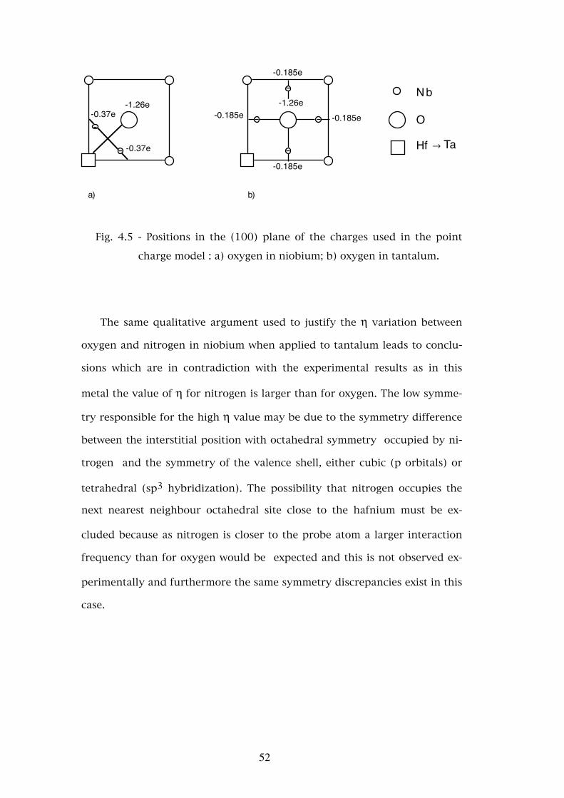
Wrede [Wrede 86] used a point charge model in order to justify the

asymmetry parameter observed in the Nb-O system. In this model a covalent

contribution to the bonding of oxygen to tantalum is considered The oxygen

bonding p electrons occupy orbitals at an angle of 90°, this situation is

simulated with two additional charges in the (100) plane at an equal dis-

tance from tantalum and from oxygen but outside the axis joining them as

is shown in Fig.4.5a. This configuration is justified by the fact that the elec-

trons will avoid the high electronic density outside this plane. Considering

the Pauling electronegativities of oxygen and tantalum [Cotton 66] the bond

between these two atoms is approximately 63% ionic and a charge of -1.26e

is localized on the oxygen atom and two charges of -0.37e are delocalized.

The experimental value of η is thus reproduced with the principal axis of

the electric field gradient (Vzz) in the <100> direction which contains the

oxygen atom, if the delocalized charges are moved towards the Ta-O axis. In

this model only the bond between the oxygen and tantalum atoms is con-

sidered. For the Ta-O system this approximation is no longer valid because

the radioactive atom 181Ta is equal to the lattice atoms. If we consider that

the p bonds are shared with the four nearest neighbours in the (100) plane

(Fig.4.5b), the value of η calculated is 0.31 close to the experimental value

of 0.35.

51

-0.185e-1.26e

-0.185e

a) b)

-0.37e

-0.37e

-0.185e

-1.26e-0.185e

Nb

O

Hf → Ta

Fig. 4.5 - Positions in the (100) plane of the charges used in the point

charge model : a) oxygen in niobium; b) oxygen in tantalum.

The same qualitative argument used to justify the η variation between

oxygen and nitrogen in niobium when applied to tantalum leads to conclu-

sions which are in contradiction with the experimental results as in this

metal the value of η for nitrogen is larger than for oxygen. The low symme-

try responsible for the high η value may be due to the symmetry difference

between the interstitial position with octahedral symmetry occupied by ni-

trogen and the symmetry of the valence shell, either cubic (p orbitals) or

tetrahedral (sp3 hybridization). The possibility that nitrogen occupies the

next nearest neighbour octahedral site close to the hafnium must be ex-

cluded because as nitrogen is closer to the probe atom a larger interaction

frequency than for oxygen would be expected and this is not observed ex-

perimentally and furthermore the same symmetry discrepancies exist in this

case.

52

4.2.3 - The temperature dependence of νQ and η

The temperature dependence of the values of νQ and η may be attrib-

uted to small changes of the charge distribution in the vicinity of the radio-

active atom. This charge distribution is altered by the increase of the ion

oscillations and by the lattice expansion. These contributions are coupled

and lead to the well known “T3/2 law” for the temperature dependence of

the electric field gradient - Vzz(T) = Vzz(T=0)(1 - B T 3/2) - [Christiansen

76]. However there is no definite trend of this dependence for impurities in

cubic metals [Witthuhn 83] which is confirmed by the present results.

Fig.4.2 shows that the behaviour of the electric field gradient strength with

temperature is different for all the systems studied. In Ta-O the variation

curve of νQ with temperature has a negative slope and a positive curvature,

in Ta-N the slope is positive and in Nb-N is approximately constant. Only in

the Nb-O system is both the slope and curvature negative and a fit of the

data to the “T3/2 law” may be done. However the value of B obtained (B=

2.7x10-6 T3/2) is one order of magnitude lower than the values obtained for

non-cubic metals [Vianden 83]. As may be seen from Fig.4.2 the negative

slope observed for the variation of νQ with temperature for oxygen is not

observed for nitrogen. The small relative variation of νQ in all systems

(smaller than 2%) indicates that the different contributions (thermal oscilla-

tions, electronic charge distribution variation and lattice expansion) either

are very small or in some way compensate each other. In the latter case

small variations in the relative values of these contributions would justify

the different behaviours observed.

Regarding the temperature dependence of η this parameter increases in

all systems with a larger variation in the case of niobium. Possibly an in-

crease of the interaction between the impurity valence electrons and the

53

metal electrons may constrain the electronic charge distribution to certain

crystal planes decreasing the charge distribution symmetry and causing an

increase in the value of η. The fact that the radioactive atom is a defect in

niobium may justify the stronger increase of η in this metal.

4.3 - Conclusions

From the perturbed angular correlation experiments made in low con-

centration alloys of niobium and tantalum with nitrogen and oxygen we

may conclude the following:

- The single and well defined interactions observed for oxygen and nitrogen

in tantalum and for oxygen in niobium, are due to trapping of one single

interstitial impurity atom and no higher order complexes are observed.

- In the Nb-N system the interaction due to one nitrogen atom is observed

and also interactions due to complexes of more than one nitrogen atom.

The formation of these complexes is strongly dependent on the nitrogen

dilution method. In order to avoid the formation of these complexes

quenching rates higher than those used for the other systems are needed.

The two additional interactions observed in this system suggest the exis-

tence of at least two distinct configurations for these complexes although

an identification of their structure has not been possible.

- Oxygen in niobium occupies an octahedral interstitial position which is

2nd nearest neighbour to hafnium and the same should hold for tanta-

lum. The present results and the models used do not allow similar con-

clusions to be made for nitrogen. The location of this atom in both the

1st or 2nd nearest neighbour position relative to hafnium is possible be-

ing excluded the simultaneous occupation of both sites as it is hard to

54

understand why only complexes of two atoms would be formed. On the

other hand the occupation of one site or the other is also excluded since

that would lead to two different electric field gradients and only one well

defined interaction is observed in both metals.

- The temperature dependence of the interaction frequencies is very small

and shows no definite trends. The larger variation of η with temperature

in niobium is attributed to the fact that 181Ta is an impurity in this

metal.

- The relative values of the electric field gradients (proportional to the in-

teraction frequencies) may be understood in terms of the valence elec-

trons of oxygen and nitrogen and of their spatial distribution relative to

the probe atom.

- The symmetry of the electric field gradient observed for oxygen in tanta-

lum and niobium may be understood in terms of a simple point charge

model involving the valence electrons of oxygen. For nitrogen a decrease

of η caused by the higher symmetry of it’s valence orbitals is expected

and is observed in niobium. The opposite behaviour observed in tanta-

lum is probably due to differences in the impurity valence orbital sym-

metry relative to it’s position in the lattice.

55

CHAPTER 5

STUDIES OF THE INTERACTION OF

HYDROGEN AND DEUTERIUM WITH OXYGEN AND NITROGEN

IN TANTALUM AND NIOBIUM

5.1 - Introduction

The trapping of hydrogen and deuterium by interstitial impurities such

as oxygen and nitrogen has been extensively studied by several methods. It

has generally been accepted that the interaction responsible for the trap-

ping of hydrogen by defects is partly due to the lattice elastic deformations

in their vicinity [Shirley 83]. The tetragonal symmetry of the deformation

field due to carbon, nitrogen and oxygen in body centered cubic metals is

well established [Shirley 83, refs Tab.1]. Quasi-elastic neutron scattering

measurements in niobium with deuterium have shown that the deformation

field for this impurity has cubic symmetry [Bauer 75]. Using inelastic X-Ray

scattering (Huang scattering) Metzger et all [Metzger 76] confirmed the

results of Bauer et all showing that the distortion field for hydrogen in nio-

bium also presents cubic symmetry. However Metzger et all [Metzger 85]

observed a tetragonal symmetry for the N-H complex in niobium indicating

56

that the symmetry of the trapping center predominates over that due to hy-

drogen.

Using electrical resistivity methods Pfeiffer and Wipf [Pfeiffer 76] and

Rosan and Wipf [Rosan 76] suggested that the reorientation of the N-H pairs

in niobium is short ranged and precipitation is suppressed when the hydro-

gen concentration is smaller than that of nitrogen. These authors also con-

cluded that only one hydrogen atom is trapped by nitrogen in niobium.

This was also observed for oxygen in niobium [Mattas 75 and Sado 82]. In-

ternal friction results showed that the trapped hydrogen position is tem-

perature dependent [Zapp 80a, Hanada 81a and 81b].

The general picture of trapping that emerges from these experimental

investigations is that a single hydrogen atom moves around on several in-

terstitial sites (tetrahedral or quasi- tetrahedral) near an immobile impurity

atom located at an octahedral site.

The structure of these complexes is still controversial. The first struc-

tures suggested by internal friction studies for the complex O-H in niobium

[Schiller 75, Zapp 80a] are in contradiction. While Schiller and Nijam sug-

gest a trigonal symmetry for the O-H pair in the <111> direction (consider-

ing hydrogen located in octahedral sites), Zapp and Birnbaum propose that

hydrogen tunnels between several interstitial positions in rings around the

oxygen atom excluding the octahedral positions and the <111> symmetry.

The structure of the N-D pair in tantalum has been studied by channel-

ing Carstanjen 80]. This system is, in principle, similar to N-H in niobium

[Rosan 76]. Carstanjen observed that nitrogen is located in an octahedral

position in tantalum and remains immobile when trapping a deuterium

atom. The trapping sites suggested for deuterium were later revised [Car-

stanjen 82] but the only safe conclusion was that the deuterium sites are not

57

located in the same face of the unit cell where the nitrogen impurity is

found.

At very low temperatures the N-H system shows an anomalous increase

of the specific heat [Morkel 78] attributed to tunneling of hydrogen between

two equivalent trapping sites close to nitrogen. This is supported by a neu-

tron diffraction experiment [Wipf 81] where the distance between the two

trapping sites was found to be around 0.1Å. In an inelastic neutron scatter-

ing study Magerl et all [Magerl 83] found that the local mode vibration en-

ergies of hydrogen in niobium are not altered when this is trapped by nitro-

gen. These authors also conclude that hydrogen remains in tetrahedral posi-

tions when trapped but at a sufficiently large distance from the trapping

center so that the hydrogen local potential remains practically undisturbed.

A N-H distance of 3.5Å was also suggested.

From these results is concluded that in the hydrogen-interstitial impu-

rity complexes configurations in niobium and tantalum hydrogen occupies

two neighbour tetrahedral sites tunneling between them. These two sites

must be 4th nearest neighbour to the interstitial impurity. At higher tem-

peratures hydrogen diffuses to the other interstitial positions available

around the trapping center until it receives enough energy to diffuse away.

5.2 - Experimental results

In the present studies of the interaction between hydrogen or deuterium

and nitrogen or oxygen the samples shown in Tab.3.2 were used. All per-

turbed angular correlation measurements were made with the samples in-

side the closed cycle helium cryostat and with the experimental system de-

scribed in chapter 3.

58

5.2.1 - The Ta-O-H(D) system

After loading Ta-ø samples with hydrogen only the well known oxygen

interaction frequency is observed at room temperature. At low tempera-

tures a new interaction frequency is observed with νQ=585MHz and η=0.72.

This interaction appears at around 55K and as may be seen in Fig.5.1, the

fraction of atoms perturbed by this interaction increases rapidly while the

fraction of atoms perturbed by oxygen decreases by the same amount when

the temperature is lowered [Peichl 83].

When deuterium is added instead of hydrogen a similar behaviour is

observed. At room temperature only the oxygen interaction is present and

at low temperatures the same interaction as for hydrogen is found. In

Fig.5.2 the temperature dependence of the fractions of atoms perturbed by

oxygen and by deuterium is presented. Although the behaviour is similar to

the previous one the new interaction appears at a higher temperature,

105K, and while for hydrogen the number of oxygen decorated atoms is

only 50% for deuterium 75% of the oxygen atoms have a trapped deute-

rium.

5.2.2 - The Ta-N-H(D) system

In this system at room temperature only the interaction due to nitrogen

is observed. At low temperatures two new interactions are observed charac-

terized by νQ1=240Mhz, η=0.80 and νQ2=250Mhz, η=0.40. The fractions of

probe atoms perturbed by these interactions are approximately equal and

disappear simultaneously at around 80K. The nitrogen interaction increases

considerably at the same temperature as can be seen in Fig.5.3. As none of

59

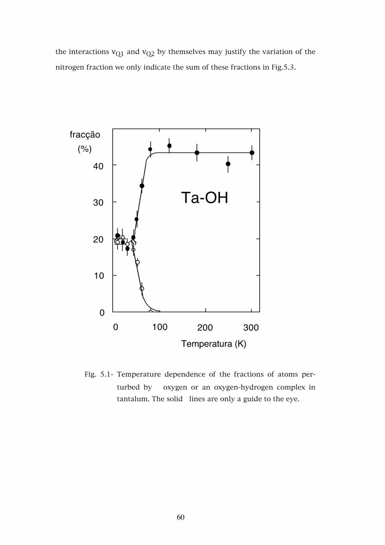
the interactions νQ1 and νQ2 by themselves may justify the variation of the

nitrogen fraction we only indicate the sum of these fractions in Fig.5.3.

Ta-OH

2001000

Temperatura (K)300

0

10

20

30

40

fracção(%)

Fig. 5.1- Temperature dependence of the fractions of atoms per-

turbed by oxygen or an oxygen-hydrogen complex in tantalum. The solid lines are only a guide to the eye.

60

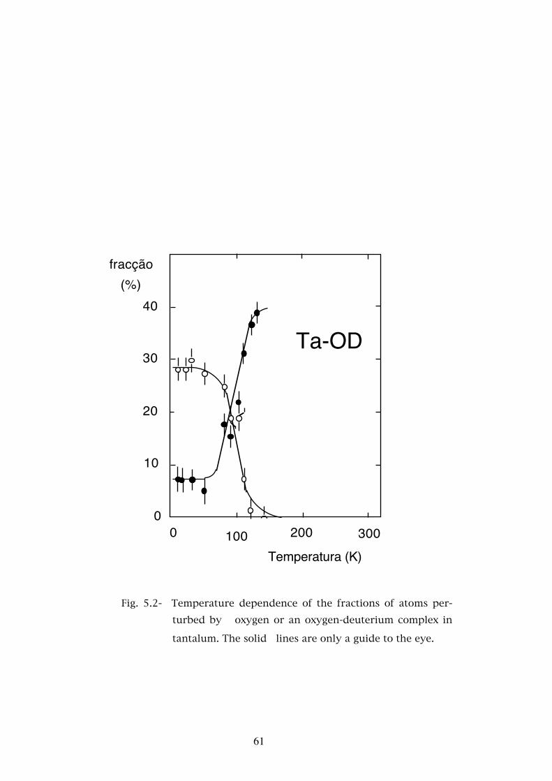
Ta-OD

2001000

Temperatura (K)

0

10

20

30

40

300

fracção(%)

Fig. 5.2- Temperature dependence of the fractions of atoms per-turbed by oxygen or an oxygen-deuterium complex in

tantalum. The solid lines are only a guide to the eye.

61

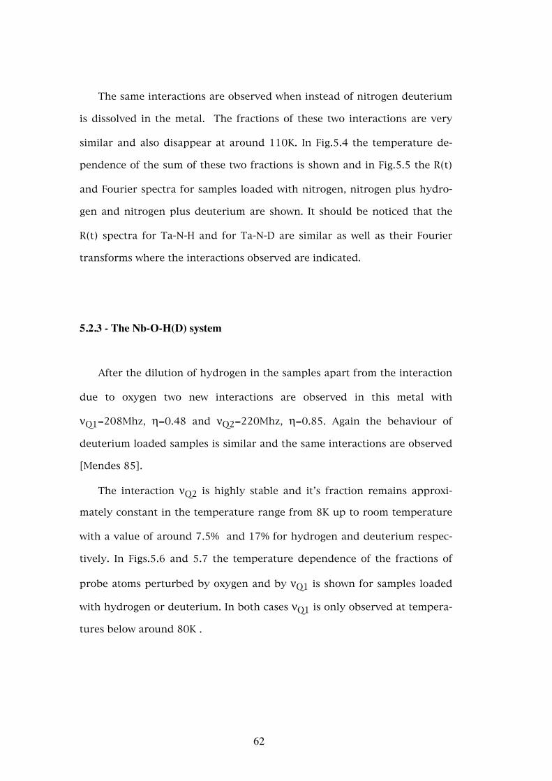
The same interactions are observed when instead of nitrogen deuterium

is dissolved in the metal. The fractions of these two interactions are very

similar and also disappear at around 110K. In Fig.5.4 the temperature de-

pendence of the sum of these two fractions is shown and in Fig.5.5 the R(t)

and Fourier spectra for samples loaded with nitrogen, nitrogen plus hydro-

gen and nitrogen plus deuterium are shown. It should be noticed that the

R(t) spectra for Ta-N-H and for Ta-N-D are similar as well as their Fourier

transforms where the interactions observed are indicated.

5.2.3 - The Nb-O-H(D) system

After the dilution of hydrogen in the samples apart from the interaction

due to oxygen two new interactions are observed in this metal with

νQ1=208Mhz, η=0.48 and νQ2=220Mhz, η=0.85. Again the behaviour of

deuterium loaded samples is similar and the same interactions are observed

[Mendes 85].

The interaction νQ2 is highly stable and it’s fraction remains approxi-

mately constant in the temperature range from 8K up to room temperature

with a value of around 7.5% and 17% for hydrogen and deuterium respec-

tively. In Figs.5.6 and 5.7 the temperature dependence of the fractions of

probe atoms perturbed by oxygen and by νQ1 is shown for samples loaded

with hydrogen or deuterium. In both cases νQ1 is only observed at tempera-

tures below around 80K .

62

Fig. 5.3 - Temperature dependence of the fractions of atoms perturbed

by nitrogen or a nitrogen-hydrogen complex in tantalum. The

solid lines are only a guide to the eye.

Fig. 5.4 - Temperature dependence of the fractions of atoms perturbed

by nitrogen or a nitrogen-deuterium complex in tantalum.

The solid lines are only a guide to the eye.

63

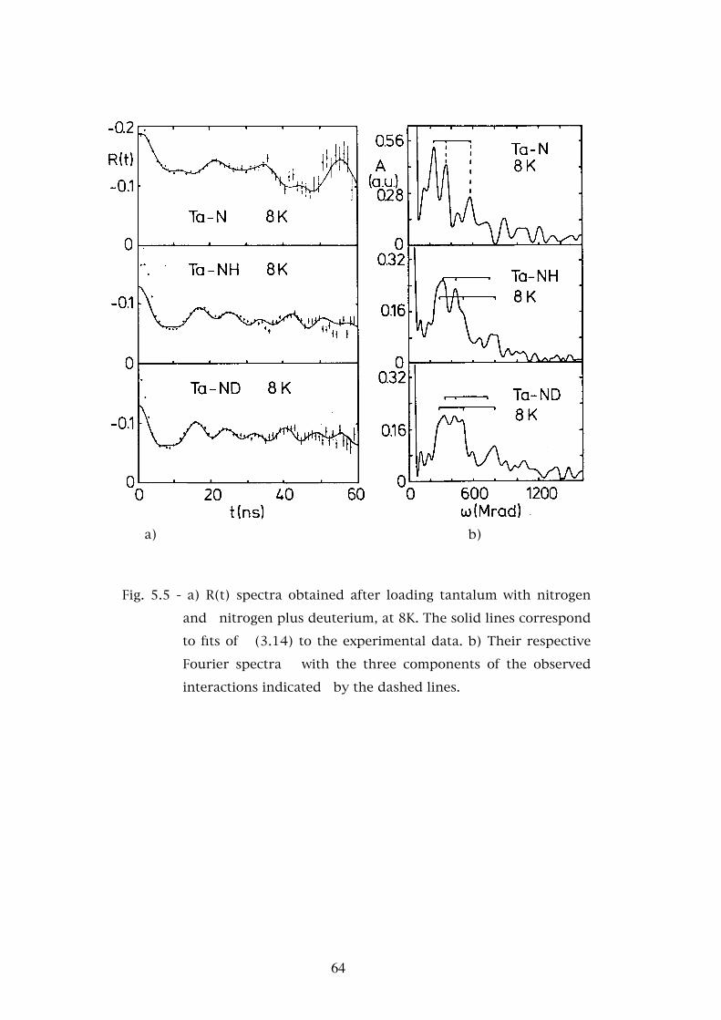
a) b)

Fig. 5.5 - a) R(t) spectra obtained after loading tantalum with nitrogen

and nitrogen plus deuterium, at 8K. The solid lines correspond

to fits of (3.14) to the experimental data. b) Their respective

Fourier spectra with the three components of the observed

interactions indicated by the dashed lines.

64

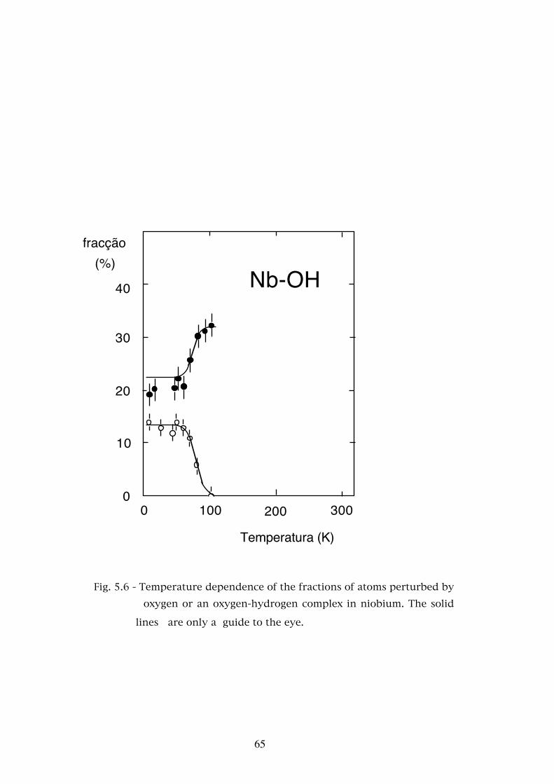
Nb-OH

200 3001000

Temperatura (K)

0

10

20

30

40

fracção (%)

Fig. 5.6 - Temperature dependence of the fractions of atoms perturbed by oxygen or an oxygen-hydrogen complex in niobium. The solid

lines are only a guide to the eye.

65

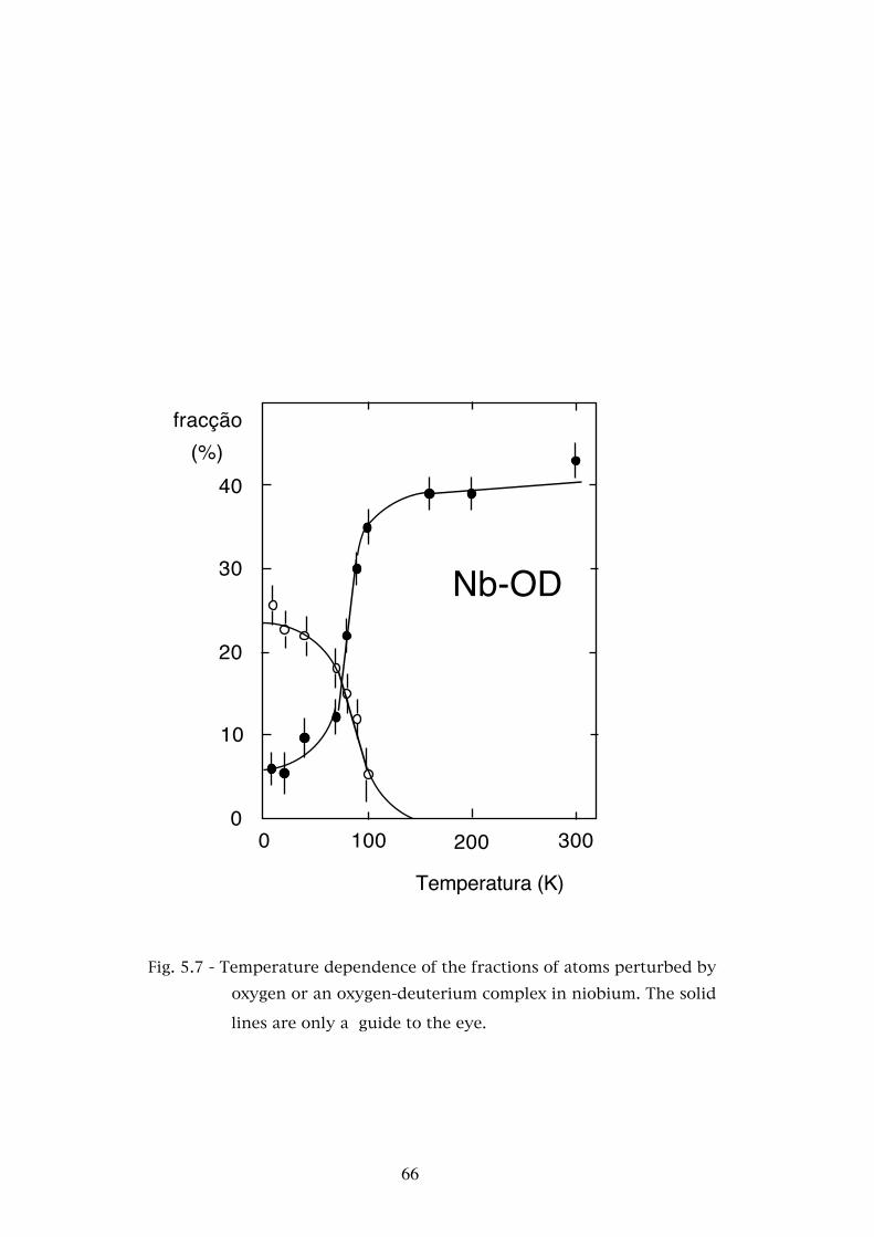
Nb-OD

10

20

30

40

0200 3001000

Temperatura (K)

fracção(%)

Fig. 5.7 - Temperature dependence of the fractions of atoms perturbed by oxygen or an oxygen-deuterium complex in niobium. The solid

lines are only a guide to the eye.

66

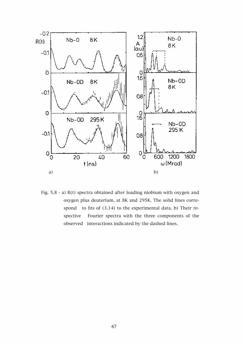
a) b)

Fig. 5.8 - a) R(t) spectra obtained after loading niobium with oxygen and

oxygen plus deuterium, at 8K and 295K. The solid lines corre-

spond to fits of (3.14) to the experimental data. b) Their re-

spective Fourier spectra with the three components of the

observed interactions indicated by the dashed lines.

67

In Fig.5.8 the R(t) spectra and their Fourier transforms after loading a

niobium sample successively with oxygen and deuterium is shown. In the

absence of deuterium only the oxygen interaction is observed. After loading

with deuterium at 295K the interaction νQ2, indicated in the Fourier spec-

trum, is also present and at 8K essentially the two interactions νQ1 and νQ2

are observed. In the Fourier spectrum corresponding to the 8K measure-

ment only the low temperature interaction νQ1 is indicated.

5.3 - Discussion

5.3.1 - Assignment of the interaction frequencies νQ

As may be seen by the present results in all the systems studied a simi-

lar behaviour is observed. There is a large decrease of the fraction of atoms

perturbed by the interaction due to oxygen (nitrogen) when the tempera-

ture is lowered and simultaneously the number of atoms perturbed by the

low temperature interaction increase by the same amount.

The interactions observed with this behaviour are summarized in

Tab.4.1. The fact that the low temperature interactions only appear in sam-

ples loaded with hydrogen (deuterium) and that they are converted to the

oxygen (nitrogen) interaction as the temperature is raised shows that they

should be due to trapping of hydrogen (deuterium) atoms by oxygen or ni-

trogen.

Due to the high hydrogen and deuterium concentrations relatively to

oxygen or nitrogen in some of the samples studied (see Tab.3.1) we would

expect to see different types of complexes due to trapping of more than one

68

atom of hydrogen (deuterium). However we only see one well defined inter-

action with this behaviour. Furthermore the trapping process is reversible

since the same transition temperatures and the same behaviour for the frac-

tions are observed when the same sample is submitted to several measure-

ment cycles wether increasing the temperature from 8K to 300K wether de-

creasing it. These facts show that the new interactions are due to trapping of

only one hydrogen (deuterium) atom in the vicinity of oxygen or nitrogen.

As was mentioned before in the Nb-O-H(D) system in addition to the in-

teractions attributed to oxygen and to the O-H(D) complex a third interac-

tion is observed νQ2=220MHz which is present at all temperatures, is iso-

tope independent and is stable in the temperature range studied. This inter-

action is not due to precipitation in ordered phases of the Nb-H system as it

was not observed in a systematic phase diagram study of this system by per-

turbed angular correlations [Mendes 83, Gil 84,87a and 87b]. In order to

clarify the origin of this interaction the sample loaded with deuterium was

submitted to an isochronal annealing programme at 400K with an angular

correlation measurement made at room temperature after each annealing

stage. In Fig.5.9 is shown the dependence on the annealing time of the frac-

tion of νQ2 which decreases linearly and vanishes after an annealing time

of 40 minutes. As this fraction decreases the fraction of the oxygen interac-

tion increases by the same amount indicating that νQ2 is converted to the

oxygen interaction by the annealing procedure. Low temperature measure-

ments after this procedure showed that the O-D interaction is still present at

80K as before and with a similar fraction.

69

Nb-O-D

0 10 20 30 40

tempo de recozimento (min )

20

10

0

fracção f3(%)

Fig. 5.9 - Fraction of probe atoms perturbed by the interaction

νQ=220MHz, η=0.85 as a function of the annealing time at 400K for a deuterium loaded sample.

From the results of this experiment we may conclude that the complex

responsible for νQ2 is very stable and dissociates irreversibly after anneal-

ing at 400K and that this complex must be due to more than one hydrogen

or deuterium atom trapped by oxygen.

The assignment of this interaction to trapping of more than one hydro-

gen atom by oxygen seems to contradict the well established fact that only

one hydrogen atom is trapped by either oxygen or nitrogen in niobium

[Pfeiffer 76, Sado 82]. This contradiction may be explained if we consider

that oxygen is not isolated in the metal but trapped in the vicinity of the

hafnium probe. This changes the potential which influences hydrogen and

may lead, under favourable conditions, to the trapping of more than one

hydrogen atom. However under normal conditions, for the concentrations,

studied the formation of these complexes is highly unlikely and will require

high local concentrations of hydrogen in the vicinity of the Hf-O complex.

As refered before in the hydrogen loading process by electrolysis the elec-

70

tric contact between the sample and the external electric circuit is made by

a gold wire in contact with the sample in several points. It is possible that

when diffusing along the preferred paths determined by this configuration

high local hydrogen concentrations exist in the sample giving rise to the

necessary conditions for the formation of these complexes. The number of

atoms affected by these complexes must therefore remain constant with

temperature, as is experimentally observed, and the dissociation process will

be irreversible since the conditions for their formation are no longer re-

peated. On the other hand as the mobility of deuterium is smaller than that

of hydrogen a greater number of probe atoms should be affected in the case

of deuterium, this is also observed experimentally. This process is not seen

in Ta-O samples which indicates that hafnium may play an important role in

the formation of these complexes favouring it in niobium.

The two interactions due to the presence of hydrogen in the Ta-N-H sys-

tem show similar behaviours, their fractions are similar and they vanish at

the same temperature. The interaction frequencies are similar (240MHz and

250MHz) however the large difference of the asymmetry parameters (0.80

and 0.40) shows that the configurations of the complexes causing these in-

teractions must be different. As both interactions are only present after

loading with hydrogen and as they are the same for deuterium they are

caused by trapping of these atoms at nitrogen. Considering that in the Ta-O-

H system trapping of hydrogen increases the value of η (Fig.5.10) and as we

expect the configuration of the N-H complex to be similar to the O-H com-

plex [Wipf 82] the interaction with η=0.80 must be due to trapping of one

hydrogen in the same position as for oxygen. The other interaction may

correspond to trapping of one hydrogen with a different configuration or

to trapping of more than one hydrogen atom.

71

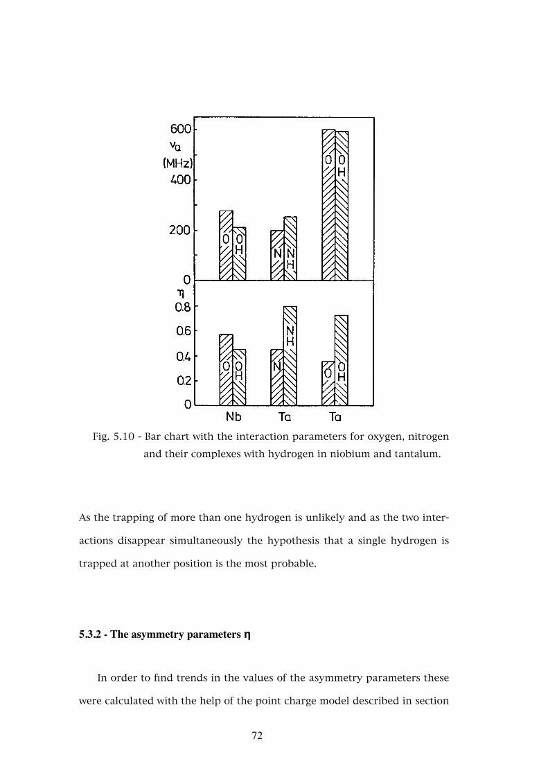
Fig. 5.10 - Bar chart with the interaction parameters for oxygen, nitrogen

and their complexes with hydrogen in niobium and tantalum.

As the trapping of more than one hydrogen is unlikely and as the two inter-

actions disappear simultaneously the hypothesis that a single hydrogen is

trapped at another position is the most probable.

5.3.2 - The asymmetry parameters η

In order to find trends in the values of the asymmetry parameters these

were calculated with the help of the point charge model described in section

72

2.5. The values for the positions and charges of oxygen in niobium and tan-

talum of the previous chapter were used and hydrogen atoms were placed

in the positions suggested by other researchers [Magerl 83] as is shown in

Fig.5.11. The charge placed in the hydrogen atom was adjusted in order to

reproduce the experimental value of η in the O-H system in niobium

(q=+0.72e). Calculations for tantalum were then performed only with a

symmetrization of the oxygen-lattice atoms bonds and leaving the rest iden-

tical. The value of η for the complex O-H obtained, η=0.82, is high relative

to the experimental value of 0.72 but the trend is correct. For any other po-

sitions of the oxygen and hydrogen atoms relative to hafnium in order that

hydrogen is 4th nearest neighbour to oxygen the value obtained for η is

always of the order of 0.35, therefore only the position indicated in Fig.5.11

may justify the large increase of this parameter. According to Tab.5.1 we

may see that, both for niobium and tantalum, the trend of the interaction

frequencies when oxygen traps hydrogen is the same as observed experi-

mentally. The point charge model fails however when the values for tanta-

lum and niobium are compared.

Nb,TaH

O

Hf

Fig. 5.11- Bcc unit cell showing the relative positions of the probe atom,

oxygen and the two tetrahedral positions occupied by hydro-gen.

73

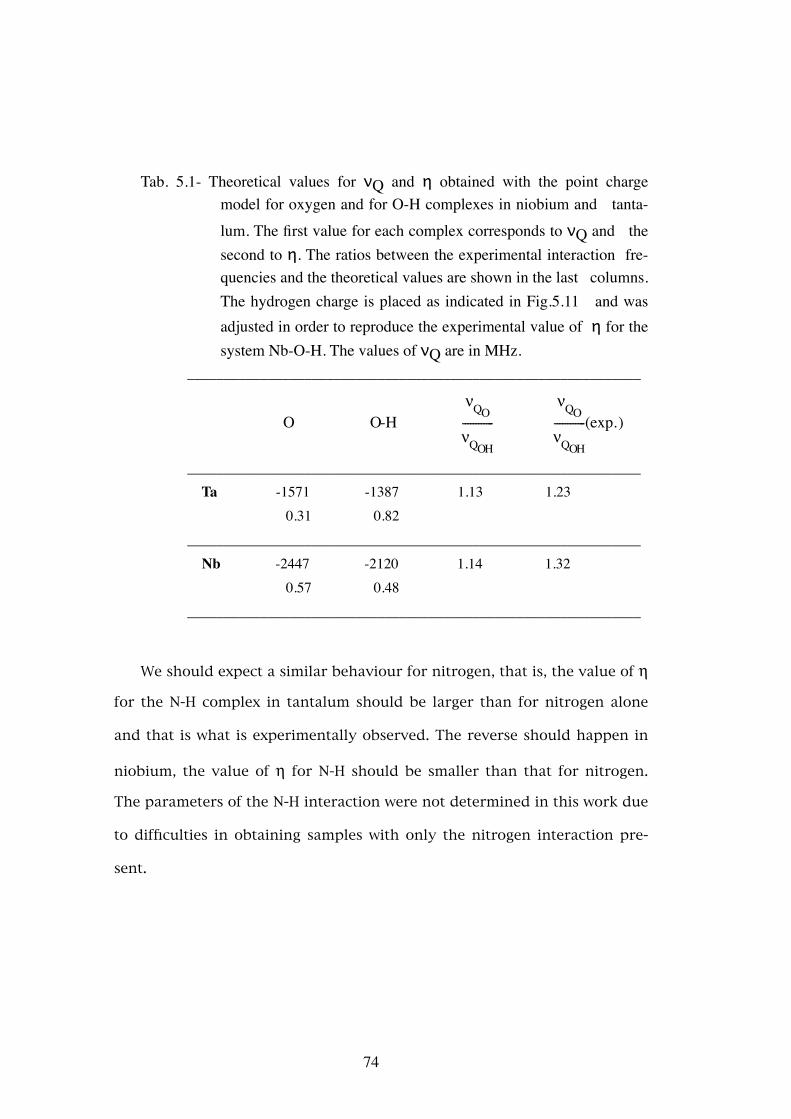
Tab. 5.1- Theoretical values for νQ and η obtained with the point charge model for oxygen and for O-H complexes in niobium and tanta-lum. The first value for each complex corresponds to νQ and the second to η. The ratios between the experimental interaction fre-quencies and the theoretical values are shown in the last columns. The hydrogen charge is placed as indicated in Fig.5.11 and was adjusted in order to reproduce the experimental value of η for the system Nb-O-H. The values of νQ are in MHz.

______________________________________________________________

O O-H ------------νQO

νQOH

------------νQO

νQOH

(exp.)

______________________________________________________________ Ta -1571 -1387 1.13 1.23 0.31 0.82______________________________________________________________ Nb -2447 -2120 1.14 1.32 0.57 0.48______________________________________________________________

We should expect a similar behaviour for nitrogen, that is, the value of η

for the N-H complex in tantalum should be larger than for nitrogen alone

and that is what is experimentally observed. The reverse should happen in

niobium, the value of η for N-H should be smaller than that for nitrogen.

The parameters of the N-H interaction were not determined in this work due

to difficulties in obtaining samples with only the nitrogen interaction pre-

sent.

74

5.3.3 - Temperature dependence of the defect fractions

The temperature dependence of the fractions of trapped hydrogen at-

oms may be interpreted in terms of trapping models. In the following sec-

tions we shall consider three distinct models.

5.3.3.a -Classical thermodynamical equilibrium

From a classical point of vue hydrogen in dilute solution in metals may

be described considering that it behaves as a gas. In the presence of trap-

ping defects the number of trapped hydrogen atoms, when thermodynami-

cal equilibrium is reached, will be a function of the defect and hydrogen

concentrations, the number of trapping sites per defect, the maximum

number of hydrogen atoms that each defect may trap and of the competi-

tion between different types of defects.

Pfeiffer and Wipf developed such a model to determine the binding en-

ergy of hydrogen to nitrogen in niobium [Pfeiffer 76]. In this model two dis-

tinct situations are considered leading to different behaviours: in the first

case the hydrogen concentration is smaller or equal to the nitrogen concen-

tration and in the second case it is larger.

When the hydrogen concentration is smaller than that of nitrogen and

the temperature is lowered all hydrogen atoms are trapped and no precipi-

tates are formed. Considering that the interstitial impurity concentrations

are very small there is no superposition of trapping sites belonging to dif-

ferent nitrogen atoms and the interaction between free hydrogens is small,

and also that only a limited number of hydrogen atoms may be trapped by

each nitrogen, the concentration ct of trapped hydrogen atoms is given by

[Pffeifer 76]:

75

ct = ------12 cH + q cN + --------

λ qz e

- ---------ε

kT

- ⎢⎡

⎣⎥⎤

⎦⎜⎛⎝ ⎟

⎞⎠ cH + q cN +--------

λ qz e

- 2

- 4 q cH cN

-------12

(5.1)⎪⎪⎧

⎩⎨ ⎪

⎪⎫

⎭⎬

---------ε

k T

where cH and cN are the hydrogen and nitrogen concentrations in the sam-

ple, q is the number of hydrogen atoms which may be trapped by each ni-

trogen, λ is the number of trapping sites per lattice atom, z is the number

of trapping sites for each nitrogen atom, ε is the binding energy of hydro-

gen to nitrogen, k is the Boltzmann constant and T the absolute tempera-

ture.

In the present work only the samples used in the study of the Nb-O-H

and Ta-N-H systems had a hydrogen concentration smaller than the intersti-

tial impurity. In both systems the temperature at which the number of

trapped hydrogen is 50% of their low temperature concentration is 80K. If

we use this value for T in (5.1) and with λ=6, z=12 and q=1, the binding en-

ergy for this concentration ratio is ε=0.028eV, much smaller than the bind-

ing energies determined by other methods for these systems; ε=0.08eV for

O-H in niobium [Hanada 81b] and ε=0.12eV for N-H in tantalum [Rosan 76].

The parameter λ corresponds to the number of interstitial tetrahedral sites

per atom in the bcc lattice. The parameter z is determined from geometrical

considerations based in the proposed trapping sites suggested by Wipf [Wipf

82]; anyway the ε dependence on z is weak and does not justify the differ-

ence between the experimental values of the binding energy and the values

calculated with this model. The value of q must be equal to unity in all sys-

tems studied. According to (5.1) the temperature dependence of the hydro-

gen concentration

76

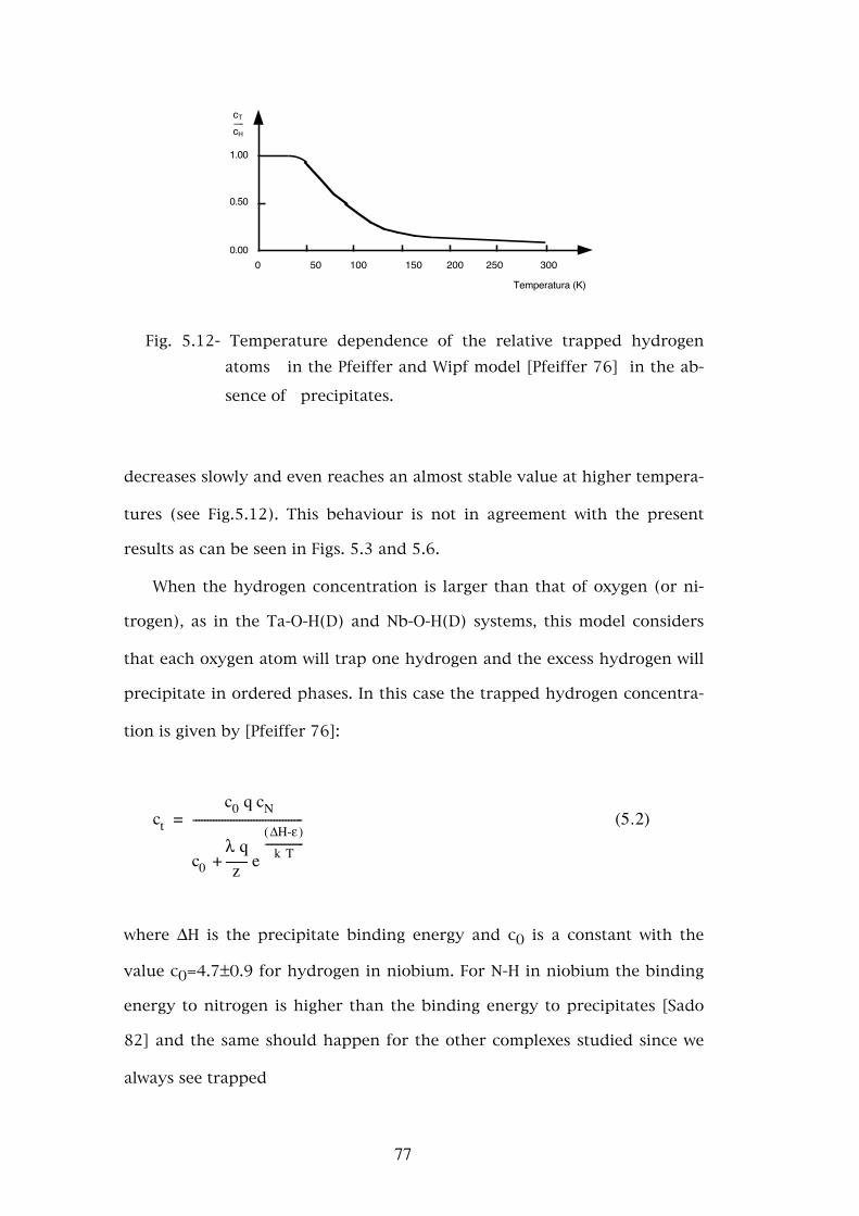
0 50 100 150 200 250 300

Temperatura (K)

0.50

0.00

1.00

------cT

cH

Fig. 5.12- Temperature dependence of the relative trapped hydrogen atoms in the Pfeiffer and Wipf model [Pfeiffer 76] in the ab-

sence of precipitates.

decreases slowly and even reaches an almost stable value at higher tempera-

tures (see Fig.5.12). This behaviour is not in agreement with the present

results as can be seen in Figs. 5.3 and 5.6.

When the hydrogen concentration is larger than that of oxygen (or ni-

trogen), as in the Ta-O-H(D) and Nb-O-H(D) systems, this model considers

that each oxygen atom will trap one hydrogen and the excess hydrogen will

precipitate in ordered phases. In this case the trapped hydrogen concentra-

tion is given by [Pfeiffer 76]:

ct = -------------------------------------- c0 q cN

c0 + --------λ qz e

--------------------------( )ΔH-ε

k T

(5.2)

where ΔH is the precipitate binding energy and c0 is a constant with the

value c0=4.7±0.9 for hydrogen in niobium. For N-H in niobium the binding

energy to nitrogen is higher than the binding energy to precipitates [Sado

82] and the same should happen for the other complexes studied since we

always see trapped

77

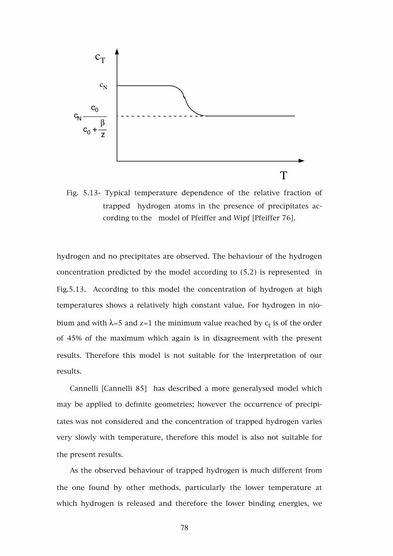
cT

cN

T

cNc0

c0 + ------βz

______

Fig. 5.13- Typical temperature dependence of the relative fraction of

trapped hydrogen atoms in the presence of precipitates ac-cording to the model of Pfeiffer and Wipf [Pfeiffer 76].

hydrogen and no precipitates are observed. The behaviour of the hydrogen

concentration predicted by the model according to (5.2) is represented in

Fig.5.13. According to this model the concentration of hydrogen at high

temperatures shows a relatively high constant value. For hydrogen in nio-

bium and with λ=5 and z=1 the minimum value reached by ct is of the order

of 45% of the maximum which again is in disagreement with the present

results. Therefore this model is not suitable for the interpretation of our

results.

Cannelli [Cannelli 85] has described a more generalysed model which

may be applied to definite geometries; however the occurrence of precipi-

tates was not considered and the concentration of trapped hydrogen varies

very slowly with temperature, therefore this model is also not suitable for

the present results.

As the observed behaviour of trapped hydrogen is much different from

the one found by other methods, particularly the lower temperature at

which hydrogen is released and therefore the lower binding energies, we

78

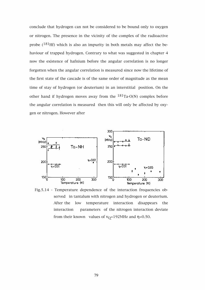
conclude that hydrogen can not be considered to be bound only to oxygen

or nitrogen. The presence in the vicinity of the complex of the radioactive

probe (181Hf) which is also an impurity in both metals may affect the be-

haviour of trapped hydrogen. Contrary to what was suggested in chapter 4

now the existence of hafnium before the angular correlation is no longer

forgotten when the angular correlation is measured since now the lifetime of

the first state of the cascade is of the same order of magnitude as the mean

time of stay of hydrogen (or deuterium) in an interstitial position. On the

other hand if hydrogen moves away from the 181Ta-O(N) complex before

the angular correlation is measured then this will only be affected by oxy-

gen or nitrogen. However after

Fig.5.14 - Temperature dependence of the interaction frequencies ob-

served in tantalum with nitrogen and hydrogen or deuterium.

After the low temperature interaction disappears the

interaction parameters of the nitrogen interaction deviate

from their known values of νQ=192MHz and η=0.50.

79

the O-H (or N-H) interaction has vanished we observe that the oxygen or

nitrogen interaction is different from it’s well known value even at high

temperatures as is shown, for instance, for the Ta-N-H(D) system in Fig.5.14.

This suggests that hydrogen is bound to the Hf-O complex before it’s decay

and that the disappearance of the low temperature interaction is related to

a rearrangement of hydrogen in the vicinity of oxygen but in a more

distant position from the radioactive atom 181Ta. It may be shown with the

point charge model that if hydrogen is released when hafnium decays, but

remains in the vicinity of oxygen occupying a position opposed to that of

hafnium, the electric field gradient due to this charge distribution is ap-

proximately the same as that created by oxygen alone. The two models pre-

sented in the next sections are based in these considerations.

5.3.3.b - Thermodynamical equilibrium with trapped hydrogen

After the previous considerations it is reasonable to suppose that the

crystal potential affecting hydrogen in the vicinity of the probe atom-

interstitial impurity has several trapping wells around oxygen and a deeper

one close to hafnium (Fig.5.15). In thermodynamical equilibrium, supposing

that for each “trapped” state bound to the Hf-O complex (i in fig.5.15) there

are s “free” states bound only to oxygen, then the probability of finding one

free hydrogen is proportional to the product of a Boltzmann factor by the

number of states available, while the probability of hydrogen being trapped

is constant:

80

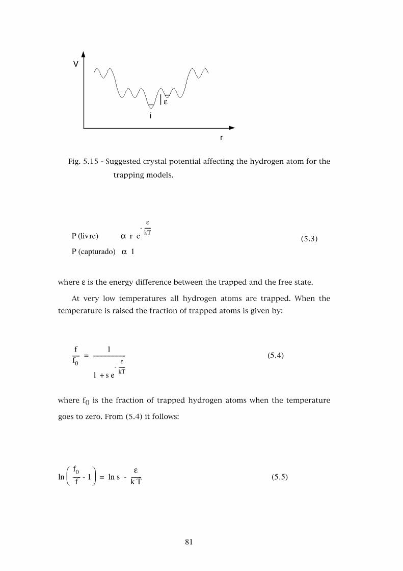
V

i

r

ε

Fig. 5.15 - Suggested crystal potential affecting the hydrogen atom for the

trapping models.

P (livre) α r e- ---------ε

kT (5.3)

P (capturado) α 1

where ε is the energy difference between the trapped and the free state.

At very low temperatures all hydrogen atoms are trapped. When the temperature is raised the fraction of trapped atoms is given by:

------ff0

= ------------------------1

1 + s e- ---------ε

kT

(5.4)

where f0 is the fraction of trapped hydrogen atoms when the temperature

goes to zero. From (5.4) it follows:

ln ⎜⎛⎝ ⎟

⎞⎠ ------

f0f - 1 = ln s - --------

εk T (5.5)

81

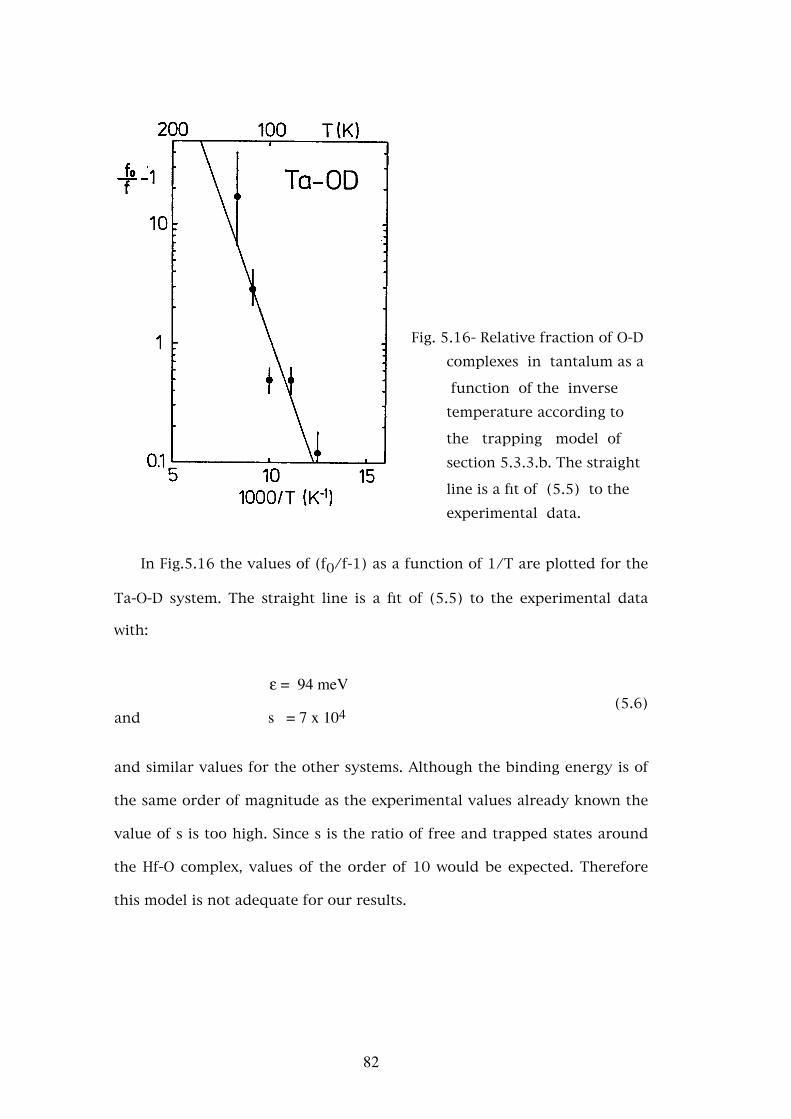
Fig. 5.16- Relative fraction of O-D complexes in tantalum as a

function of the inverse temperature according to

the trapping model of section 5.3.3.b. The straight

line is a fit of (5.5) to the experimental data.

In Fig.5.16 the values of (f0/f-1) as a function of 1/T are plotted for the

Ta-O-D system. The straight line is a fit of (5.5) to the experimental data

with:

ε = 94 meV (5.6)and s = 7 x 104

and similar values for the other systems. Although the binding energy is of

the same order of magnitude as the experimental values already known the

value of s is too high. Since s is the ratio of free and trapped states around

the Hf-O complex, values of the order of 10 would be expected. Therefore

this model is not adequate for our results.

82

5.3.3.c - Hydrogen released by the nuclear decay

In the previous model the decay of hafnium does not alter the crystal

potential of Fig.5.15 affecting hydrogen. In this model we shall suppose that

trapping of hydrogen close to hafnium only exists before the decay and that

hafnium releases hydrogen of the trapped state after decay. This is equiva-

lent to the disappearance of the potential well i in Fig.5.15 after the decay.

If we assume that the probability of hydrogen remaining in the same posi-

tion after the decay varies exponentially with time:

P (t=0) = 1

(5.7)

e P (t=t) = e- -------

t

τ_

Where τ is the mean time of stay of hydrogen in a trapped position at the

temperature T, Then the probability that, when the angular correlation is

observed at time t, hydrogen is still trapped is given by:

P0 (t) = e- -------

t

τ --------------- e

− ----------t

τΝ

τN

(5.8)_

where (1/tN e-t/τN ) is the probability of detecting the second γ-ray at the

time t after hafnium decays with τN the lifetime of the 181Ta excited state

populated by the hafnium decay.

83

In the region of temperatures where the hydrogen or deuterium interac-

tion vanishes, the ratio between this fraction and it’s value for very low

temperatures f/f0 is given by the integral of P0(t) from 0 to ∞:

------ff0

= ------1τN

⎮⎮⎮⎮⌠

⌡0

∞

e- -------

t

τ e- ---------

t

τN dt (5.9)_

calculating the integral in (5.9) we get:

------ff0

= --------------τ

τ + τN

(5.10)_

_

from where follows:

τ = ---------------τN

------ff0 - 1

(5.11)_

If we assume that τ has an Arrhenius behaviour in this temperature range:

τ = τ∞ e----------ε

κΤ (5. 12)_

we find:

------------------------ 1

------f0f - 1

= ------τ∞τN

e---------ε

kT (5.13)

From where we find:

84

ln ⎜⎛⎝ ⎟

⎞⎠------

f0f - 1 = ln ------

τN

τ∞ - --------

εk T (5.14)

From (5.14) values for the binding energy ε and for the time of stay τ∞

of hydrogen (deuterium) when the temperature goes to infinity can be ob-

tained. In Tab.5.2 values for ε and τ∞ calculated with (5.14) for the systems

studied are presented. In Figs.5.17 and 5.18 the dependence of τ as a func-

tion of 1/T obtained experimentally are plotted against the known values

for hydrogen and deuterium in tantalum and niobium [Qi 83]. The dashed

lines are an extrapolation from the high temperature region.

The values of ε and τ∞ obtained with oxygen and nitrogen in tantalum

are similar for the two isotopes which indicate that both atoms create simi-

lar potentials. The values of ε and τ∞ in niobium are identical as is expected

from the similar behaviour of these two systems. The activation energies

obtained with this model correspond to approximately 30-50% of the

binding energies to oxygen or nitrogen in pure systems.

85

Tab. 5.2- Energy activation ε and time of stay τ∞ when T goes to ∞ for the nuclear model of section 5.3.3.c.

_________________________________________________

ε τ∞ (mev) (10-9s)________________________________________________________

Nb � H(D)� 39 ± 23 � 155 ± 16

________________________________________________________

Ta � H � 28 ± 4 � 62 ± 2� D � 57 ± 18 � 32 ± 1________________________________________________________

Fig. 5.17- Values for the mean time of stay of hydrogen and deuterium

trapped by oxygen (black symbols) and by nitrogen (white

symbols) in tantalum according to the nuclear model of section

5.3.3.c compared with the diffusion data available. The dashed

lines are extrapolations of the high temperature data.

86

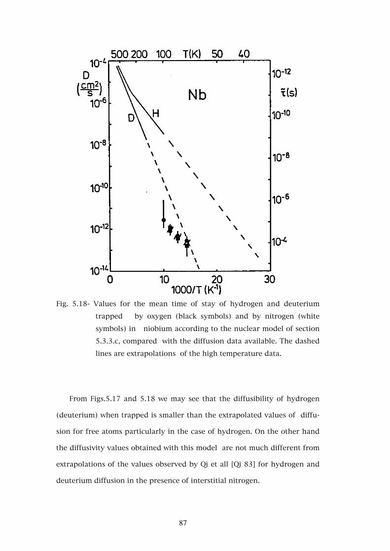
Fig. 5.18- Values for the mean time of stay of hydrogen and deuterium

trapped by oxygen (black symbols) and by nitrogen (white

symbols) in niobium according to the nuclear model of section

5.3.3.c, compared with the diffusion data available. The dashed

lines are extrapolations of the high temperature data.

From Figs.5.17 and 5.18 we may see that the diffusibility of hydrogen

(deuterium) when trapped is smaller than the extrapolated values of diffu-

sion for free atoms particularly in the case of hydrogen. On the other hand

the diffusivity values obtained with this model are not much different from

extrapolations of the values observed by Qi et all [Qi 83] for hydrogen and

deuterium diffusion in the presence of interstitial nitrogen.

87

5.4 - Conclusions

From the studies of hydrogen and deuterium complexes with oxygen

and nitrogen in niobium and tantalum we may conclude that:

- Under normal circunstances only one hydrogen or deuterium atom is

trapped by the interstitial impurities oxygen and nitrogen confirming the

results of other experiments with macroscopical techniques.

- In niobium the temperature at which these interactions vanish is the same

for both isotopes. This behaviour is attributed to the fact that, as oppo-

site to tantalum, both the probe atom and the product of it’s decay are

impurities in this metal.

- In some systems other interactions are observed also due to hydrogen and

with similar behaviour for the two isotopes. In the Nb-O system an inter-

action is observed which is due to meta-stable hydrogen complexes

formed during the electrolytical loading and which disappear after an-

nealing at 400K. In the Ta-N system one interaction probably due to a

different configuration of the N-H(D) complex is also observed.

- The relative values of the η parameter for the O-H(D) complex interaction

in tantalum may be understood in terms of a simple point charge model

if we consider the covalent bonding charges of oxygen delocalized and

oriented according to the crystal symmetry. This model agrees with the

positions suggested for hydrogen by other researchers [Wipf 82, Magerl

83] with hydrogen occupying tetrahedral sites 4th nearest neighbours to

oxygen or nitrogen.

- It was not possible to identify the interaction due to the N-H complex in

niobium since we were unable to isolate the nitrogen interaction. Sup-

pression of the interactions due to complexes of more than one nitrogen

88

requires changing the loading procedure in order to achieve higher

cooling rates to freeze the random distribution of nitrogen atoms in the α

phase and preventing precipitates.

- Trapping models were used for the interpretation of the temperature de-

pendence of the fractions of hydrogen atoms trapped. The classical point

of vue of thermodynamical equilibrium between trapped and free states

is unable to describe the present results as the binding energies calcu-

lated are very low when compared to results of other techniques and also

because the temperature dependence of the fractions of trapped atoms is

in disagreement with experiment. The results were therefore interpreted

in terms of hydrogen diffusing away from the radioactive probe but re-

maining in the vicinity of the interstitial impurity. In particular we find

values of the mean time of residence for these atoms which are between

extrapolations of high temperature data of the metal-hydrogen pure sys-

tems and the metal-hydrogen(deuterium)—oxygen(nitrogen) systems.

89

CHAPTER 6

FINAL REMARKS

The results of the present work show that the perturbed angular correla-

tion method may be used for the study of hydrogen in metals with some ad-

vantages over the more common macroscopic methods. The identification of

each type of defect by a unique interaction allows the study of it’s evolution

even when other interactions are present. This feature was used successfully

in the present work in the studies of the Nb-O-H(D) systems.

However when the number of interactions, or types of defects, is high as

in the Nb-N-H(D) systems the fitting procedures of the theoretical perturba-

tion function to the experimental data becomes difficult not allowing a

unique attribution of the interactions present. The possibility of hydrogen

being captured by each of the three types of defects observed in the Nb-N

system, with the possibility of the existence of different configurations for

the same defect, leads to a large number of interactions which difficults the

unambiguous and coherent fit of the different experimental spectra.

The identification and study of the interaction due to the N-H complex

in niobium is interesting since this is one of the most extensively studied

systems. For this purpose a better control of the nitrogen dilution in nio-

bium is necessary in particular the cooling rate must be fast enough to

90

quench the random solution of nitrogen atoms in the metal without the

occurrence of precipitates.

Although the present results agree with the position of hydrogen rela-

tive to oxygen or nitrogen as suggested by Magerl et all [Magerl 83] for

niobium (according to the calculations of the point charge model), it would

be interesting to investigate the symmetry of these defects by studying them

in single crystals. The Ta-O-H system is the most convenient for these stud-

ies as it is easy to prepare and the only interactions observed are due to

oxygen and to the O-H complex. Furthermore the probe atom after the de-

cay is similar to the lattice atoms. However this experiment involves the im-

plantation of the radioactive species in a tantalum single crystal.

Within the scope of this project studies of inelastic X-Ray scattering in

the Ta-O-H system are planned. This method has recently been used to

study the symmetry and lattice distortions caused by N-H complexes in nio-

bium [Metzger 85].

As a natural development of the hydrogen in metals project in which

this work is included studies of perturbed angular correlations in hydrogen-

ated alloys of technological importance such as LaNi5 and FeTi is being

planned.

91

APPENDIX A

THE PERTURBED ANGULAR CORRELATION AND

THE ELECTRIC HYPERFINE INTERACTION

A.1 - The Perturbed Angular Correlation

The general form of the angular correlation between two γ rays emitted

successively by an excited nucleus in the absence of extra nuclear perturba-

tions (fig.2.1) is given by [Frauenfelder 65]:

W (k1 ,k2) = ∑mi ma mb

<mf|H2|mb><ma|H 1|mi> δmamb

<mf|H2|m'a >*<m'b |H1|mi>* δm'am'b

m' a m'b mf

(A.1)

×

×

where the Hamiltonians H1 and H2 describe the interaction of the nucleus

with the radiation field. Without extra nuclear perturbations during the life-

time of the intermediate state the final eigenstates |ma>, |m’a> after the

emission of γ1 are identical to the initial eigenstates |mb>, |m’b> of the sec-

ond radiation γ2.

We now consider that the nucleus is no longer isolated but interacts

with an extra nuclear electromagnetic field. This interaction, characterized

by an Hamiltonian K, will affect the nucleus during the time interval be-

92

tween the emission of γ1 (t=0) and the emission of γ2 (t=t). During this time

interval the external field interacts with the nuclear moments of the inter-

mediate state giving rise to transitions from the magnetic substates |ma> to

different substates |mb>. The time evolution of these states is represented

by a unitary operator Λ(t) satisfying Schrödinger equation:

------∂∂t Δ (t) = - ------

ih K Δ (t) (A.2)

For time independent interactions, K does not depend on time and the

solution to (A.2) is simply:

Δ (t) = e- -------

ih

K t (A.3)

Therefore the perturbed angular correlation is given by:

× <mf|H 2Δ(t)|m'a >* <m'a |H1|mi>*ma m'a

mi mfW (k1,k2) = ∑ <mf|H2Δ(t)|ma><ma|H1|mi> × (Α. 4)

The states |m> form a complete set and the state vector Λ(t) |ma> may

be expanded in terms of this base:

Δ (t) |ma> = ∑mb

|mb><mb| Δ(t) |ma>

(A.5)

Δ (t) |m' a> = ∑m'b

|m' b><mb| Δ(t) |ma>

93

After this expansion the angular correlation may be written:

W (k1 ,k2 ,t) = ∑mi mf

m a m 'am b m' b

<mf| H2 |mb ><mb| Δ(t) |ma><ma | H1 |mi> × (Α. 6)

× <mf| H2 |m' b>*<m b| Δ(t) |m' a>*<m' a| H1 |mi>

*'

A comparison of (A.1) with (A.6) shows that the perturbed angular cor-

relation may be written as the product of the matrix elements of the unper-

turbed correlation by time dependent matrix elements describing the influ-

ence of the extra nuclear interaction on the angular correlation.

Finally the perturbed angular correlation (A.6) may be conveniently

written:

W (k1,k2,t) = Gk1k2

N1 N2 (t) [ ]( )2k1+1 (2k2+1)-------12 Yk1

N1*(θ1,ϕ

1) Yk2

N2*(θ

2,ϕ

2)∑

k1 k2N1 N2

Ak1(1) Ak2

(2)

(A.7)

with the perturbation factor given by:

× <mb|Δ(t)|ma><m'b |Δ(t)|m'a >* (A.8)

Gk1k2

N1N2 (t) = ∑ma mb

(-1)2I+ma+mb [(2k1+1)(2k2+1)]2 ⎜

⎛⎝

⎟⎞⎠

Im'a

I-m

k1N1

⎜⎛⎝

⎟⎞⎠

Im'b

I-mb

k2N2

×1

a

where k1 and k2 are the multipolarities allowed for γ1 and γ2, (θ1,ϕ1) and

(θ2,ϕ2) are the Euler angles for the directions k1 and k2 as indicated in

fig.A.1. For vanishing perturbation (t=0) the evolution matrix Λ(t) reduces

to the unit matrix and the orthogonal relations of the 3-j symbols gives:

94

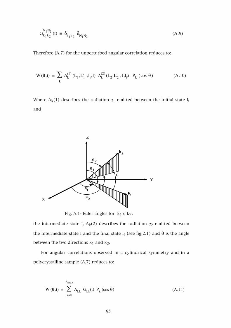
Gk1k2

N1N2 (t) ≡ δk1k2 δN1N2

(A.9)

Therefore (A.7) for the unperturbed angular correlation reduces to:

W (θ, t) = ∑k

Ak(1) (L1,L'1 ,Ii,I) Ak

(2) (L2,L'2 ,I,If) Pk (cos θ ) (A.10)

Where Ak(1) describes the radiation γ1 emitted between the initial state Ii

and

X

Y

Z

θ

θ1

2θ

ϕ2

ϕ1

k2

k1

Fig. A.1- Euler angles for k1 e k2.

the intermediate state I, Ak(2) describes the radiation γ2 emitted between

the intermediate state I and the final state If (see fig.2.1) and θ is the angle

between the two directions k1 and k2.

For angular correlations observed in a cylindrical symmetry and in a

polycrystalline sample (A.7) reduces to:

W (θ, t) = ∑k=0

kmax

Akk Gkk(t) Pk (cos θ) (Α. 11)

95

where Akk=Ak(1)Ak(2).

A.2 - The Electric Quadrupole Interaction

To determine the matrix elements of the perturbation in (A.8) a knowl-

edge of the electrostatic Hamiltonian, Hel, responsible for the hyperfine

interaction is essential.

A.2.1 - Classical Hyperfine Interaction

The electrostatic energy of the nuclear charge, described by ρn(r) under

the influence of the potential V(r), created by the electrons and the lattice

charges, is given by:

W = ∫ ρn (r) V (r) dτ (A.12)with

Z e = ∫ rn(r) dt (A.13)

the total nuclear charge.

Assuming that V(r) changes slowly in the region where ρn(r) is non

vanishing it may be expanded in a Taylor series in the vicinity of r=0:

V (r) = V(0) + ∑α= 1

3

⎜⎛⎝

⎟⎞⎠

---------∂V∂x

α 0

+ ------12 ∑

α=1

3

β=1

⎜⎜⎛

⎝

⎟⎟⎞

⎠-----------------∂

2v

∂xα∂x

β 0

xα xβ + . . . (A.14)

Inserting (A.13) and (A.14) in (A.12) the electrostatic energy is given by:

96

W = V0 Z e +∑α=1

3

⎜⎛⎝

⎟⎞⎠

---------∂V∂x

α 0

∫ ρn(r) xαd τ + ------

12 ∑

α=1β=1

3

⎜⎜⎛

⎝⎟⎟⎞

⎠-----------------∂2 V∂x

α∂x

β 0

∫ ρn (r)xαxβdτ + . . . (A.15)

The first term is the Coulomb energy of a point charge, which only con-

tributes to the potential energy of the lattice and therefore has no relevance

on the discussion of hyperfine interactions. The second term corresponds to

the dipole interaction which vanishes for nuclear states with a well defined

parity since the dipole moment for these states is zero. The third term in-

cludes the isomeric shift and the quadrupole interaction.

With r2=∑xα2 the third term may be written as follows

W = ------16 ∫ ρn(r)r2dτ ∑

α=1

3

β=1

⎜⎜⎛

⎝⎟⎟⎞

⎠-----------------∂2V∂x

α∂x

β0

+ ------16 ∑

α=1

3

β=1

⎜⎜⎛

⎝

⎟⎟⎞

⎠-----------------∂

2V

∂xα∂x

β 0

∫ ρn(r)(3xα

xβ-r2δ

αβ) dτ (A.16)

The second derivatives (∂2V/∂xα∂xβ)=qαβ form a symmetric (3x3) matrix

which may be diagonalized by a convenient rotation of the coordinate sys-

tem. Performing this rotation on the first term of (A.16) and considering

that the electrostatic potential V(r) obeys the Poisson equation ΔV=-4πρe(r),

where ρe(r) is the electronic charge density, in holding particularly for r=0

we get:

(ΔV)0 = ∑ qαα = 4 π e | ψ(0) |2 (A.17)

where e|ψ(0)|2 is the charge density of the electrons inside the nucleus.

The electrostatic hyperfine interaction is therefore:

97

W = ---------2πe3 ⎪Ψ(0)⎪

2 ⎮⎮⎮⎮⌠

⌡ ρn(r) r2 dτ + ------

16 ∑

α=1

3

β=1

⎜⎜⎛

⎝⎟⎟⎞

⎠-----------------∂2φ

∂xα∂x

β0

⎮⎮⎮⎮⌠

⌡ ρn(r) (3x

αxβ-r2δ

αβ) dτ

(A.18)

≡ V (I) + V(Q)

The isomeric shift V(I) reflects the interaction between the extended

charge of the nucleus and the electronic density at the nucleus.

The quadrupole term V(Q) gives the interaction between the electric

field gradient tensor and the quadrupole moment tensor which describes

the non spherical nuclear charge distribution.

A.2.2 - Quantum Mechanical treatment of the Electrostatic Hyperfine Interaction

The nuclear eigenstates may be characterized by the angular momen-

tum quantum numbers I and m. In this representation the energy of the

electrostatic interaction is given by the matrix element of the Hamiltonian:

Em = < Im | Hel | Im > (A.19)

with

Hel = ∑n,e

-------------------ρnρe

⎪rn - re⎪ (A.20)

the sum is extended to all the nuclear, n, and extra nuclear, e, charges

(fig.A.2).

Expanding (A.20) in Legendre polinomials

98

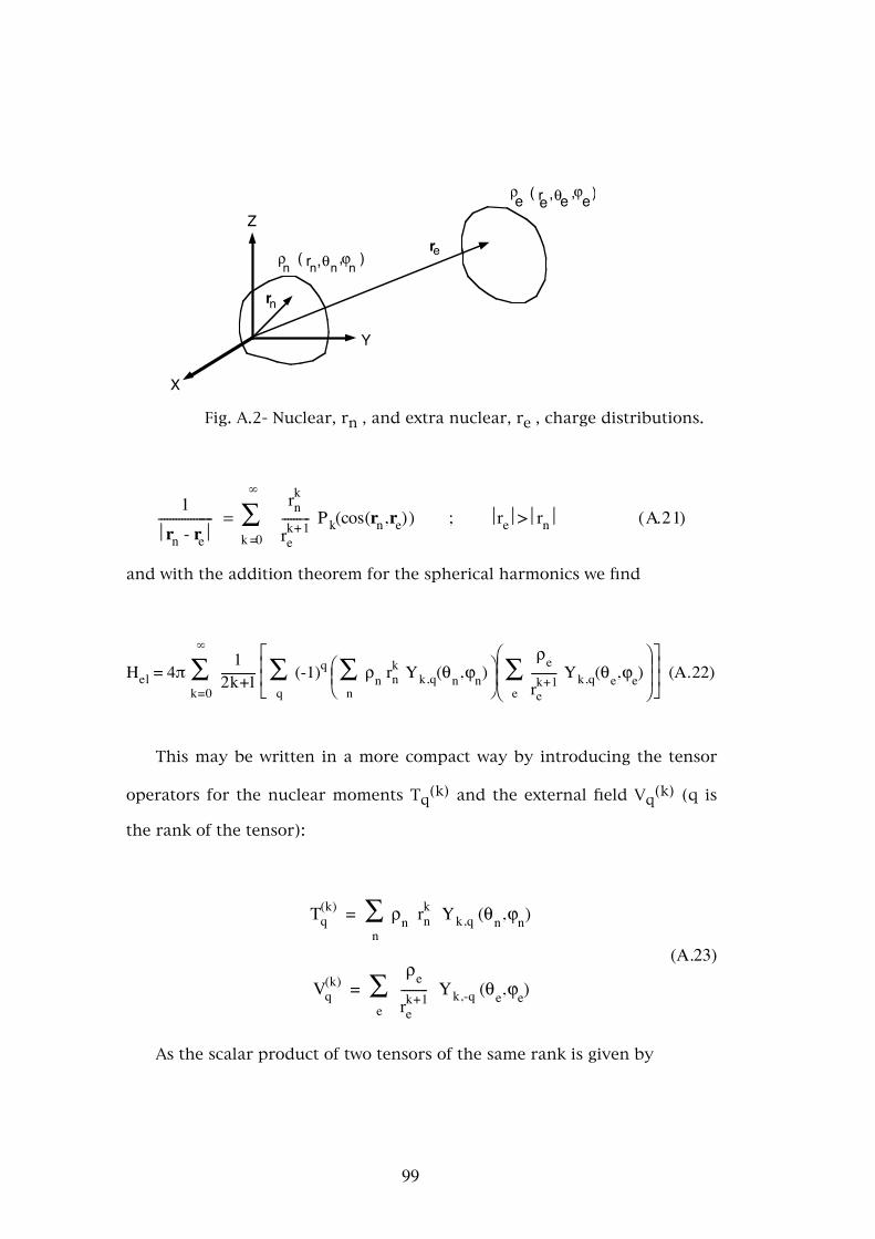
X

Y

Z

nnnnρ ( r ,,θ ϕ )

ρ ( r ,,θ ϕ )e ee e

re

rn

Fig. A.2- Nuclear, rn , and extra nuclear, re , charge distributions.

-------------------1

⎪rn - re⎪ = ∑

k =0

∞

---------rnk

rek+1 P k(cos(rn,re)) ; ⎪re⎪>⎪rn⎪ (A.21)

and with the addition theorem for the spherical harmonics we find

Hel = 4π ∑k=0

∞

------------1

2k+1 ⎢⎢⎡

⎣⎥⎥⎤

⎦∑

q (-1)q ⎜

⎛⎝

⎟⎞⎠

∑n

ρn rnk Yk,q(θn,ϕn) ⎜

⎜⎛

⎝⎟⎟⎞

⎠∑

e ---------ρe

rek+1 Yk,q(θe,ϕe) (A.22)

This may be written in a more compact way by introducing the tensor

operators for the nuclear moments Tq(k) and the external field Vq(k) (q is

the rank of the tensor):

Tq(k) = ∑

n

ρn rnk Yk,q (θn,ϕn)

(A.23)

Vq(k) = ∑

e ---------ρe

rek+1 Yk,-q (θe,ϕe)

As the scalar product of two tensors of the same rank is given by

99

T(k) V(k) = ∑q=-k

+k

(-1)q Tq(k) Vq

(k) (A.24)

the Hamiltonian may be written

Hel = ∑k=0

∞

------------4π

2k+1 T(k) V(k) = 4π ⎢⎢⎡

⎣ -------Z e4π V(0) + ------

13 ∑

q=-1

+1

(-1)q Tq(1) Vq

(1) +

+ ⎥⎥⎤

⎦------15 ∑

q=-2

+2

(-1)q Tq(2) Vq

(2) + ------17 ∑

q=-3

+3

(-1)q Tq(3) Vq

(3) + . . . (A.25)

The first term is the Coulomb term. The expectation values of T(1) (elec-

tric dipole moment) and of T(3) (electric quadrupole moment) are zero.

Higher order moments are usually very small and can be neglected. We are

therefore left with the Hamiltonian operator for the electric quadrupole in-

teraction:

Hel = ------4π5 T(2) V(2) = ------

4π5 ∑

q=-2

+2

(-1)q Tq(2) Vq

(2) (A.26)

The electric field gradient tensor V(2) can be expressed in an arbitrary

cartesian coordinate system (x’,y’,z’). Taking into account it’s symmetry

Vα'β' = -----------------

∂2V∂α' ∂β'

= Vβ'α' (A.27)

and Laplace’s equation ΔV = 0 (considering only the charge distribution

which is external to the nucleus) only five independent components remain

expressed as:

100

V0(2) = ------

14 ------

5π Vz'z'

V±1(2) = -+ ------

12 ------

56π ( )Vx'z' -+ i Vy'z' (A.28)

V±2(2) = ------

14 ------

56π (Vx'x' - Vy'y' ± 2Vx'y')

The number of components may be further reduced by a suitable trans-

formation to the principal axis

V0(2) = ------

14 ------

5π Vzz

V±1(2) = 0 (A.29)

V± 2(2) = ------

14 ------

56π (Vxx - Vyy)

If we define η=(Vxx-Vyy)/Vzz the electric field gradient is characterized

as well by the parameters Vzz and η. With the convention |Vxx|≤|Vyy|≤|Vzz|

the asymmetry parameter η has values in the range 0≤η≤1.

When the field gradient has axial symmetry, as for hexagonal or

tetragonal lattices, the components Vxx and Vyy are equal and the electric

field gradient is given by

V0(2) = ------

14 ------

5π Vzz (A.30)

And the Hamiltonian reduces to:

101

Hel = ------π5 T0

(2) Vzz (A.31)

with the quadrupole interaction energy given by:

Em = <Im| ΗQ|Im> = ------π5 Vzz <Im| T0

(2) |Im> (A.32)

The quadrupole moment of the nucleus is defined as the maximum Z

component (I=m) of the quadrupolar tensor

e Q = <II|∑n

ρn(3z2n-r2

n) |II> = 4 ------π5 Vzz <Im| T0

(2) |Im> (A.33)

Using the Wigner-Eckart theorem (A.32) and (A.33) become:

Em = (-1)I-m ------π5 Vzz ⎛⎝

⎞⎠

I-m 20 I

m <I || T(2) || I> (A.32a)

e Q = 4 ------π5 ⎛⎝

⎞⎠

I-I

20 II <I || T(2) || I> (A.33a)

Where < I || T(2) || I > is the reduced matrix element of the quadrupole mo-

ment operator.

By replacing (A.33a) in (A.32a) and evaluating the 3-j symbols we find

for the quadrupole interaction energies of the m states:

Em = -----------------------------3m2 - I(I+1)

4I (2I-1) e Q Vzz (A.34)

102

From the properties of the 3-j symbols it follows that Em=0 for I<1 and

Em≠0 for I>1. As the energies depend on m2 there remains a twofold degen-

eracy of the m states and the splitting between these substates is not equi-

distant.

The difference in energy between two substates m and m’ is given by:

Em - Em' = ----------------------3 e Q Vzz4I (2I-1) ⎪m2 - m' 2⎪ (A.35)

If we define the quadrupole frequency as:

ωQ = -------------------------e Q Vzz

4I (2I-1) h (A.36)

we get:

Em - Em' = 3 h ωQ | m2 - m'2 | (A.37)

The transition frequency ω0 corresponding to the smallest measurable

energy difference is:

ω0 = 3 ωQ for I integer

(A.38)

ω0 = 6 ωQ for I half-integer

A.2.3 - The Perturbation Factor for the Electric Quadrupole Interaction

The matrix elements <mi|L(t)|mj> of the perturbation factor (A.8) can be

calculated if we replace K in (A.3) by the Hamiltonian Hel (A.31):

103

<mb|Δ(t)|ma> = <mb|e- -------

ih

Hel t|ma> = e

- -------ih

Emb t δmamb

(A.39)

and similarly for m’a and m’b. The perturbation factor is only non vanishing

for ma=mb=m and m’a=m’b=m’ and is given by:

Gk1k2NN (t) = ∑

m, m'[ ](2k1+1)(2k2+1)

-------12 ⎜⎛⎝ ⎟

⎞⎠

Im'

I-m

k1N

⎜⎛⎝ ⎟

⎞⎠

Im'

I-m

k2N

e- -------

ih

(Em-Em') t (A.40)

For an axial symmetric field gradient with the energy differences Em-Em’

given by (A.37) the perturbation factor is:

Gk1k2NN (t) = ∑

n SnN

k1k2 cos (n ω0 t) (A.41)

where n is a positive integer (including 0) with values |m2-m’2| and 1/

2|m2-m’2| for integer and half-integer I respectively. The coefficients Sk1k2

nN

SnNk1k2 = ∑

m, m' [(2k1+1)(2k2+1)]

-------12 ⎜⎛⎝ ⎟

⎞⎠

Im'

I-m

k1N

⎜⎛⎝ ⎟

⎞⎠

Im'

I-m

k2N

(A.42)

For polycrystalline samples the angular correlation is obtained by aver-

aging over all the directions of the microcrystals symmetry axes. The per-

turbation factor is given by:

Gkk(t) = ∑n

skn cos (n ω0

t) (A.43)

with

104

skn = ∑m, m'

⎛⎝⎞⎠

Im'

I-m k

-m+m' ; s00 = 1 (A.44)

where n has the same values as for (A.41). Numerical values for skn are

tabulated for several values of the intermediate spin I in [Frauenfelder 65].

For a non-axial electric field gradient (η≠0) it is necessary to diagonalize

the Hamiltonian Hel for each value of η. The perturbation factor can still be

written as in (A.43) but the skn coefficients and transition frequencies de-

pend on the value of η:

Gkk (t) = ∑n

skn (η) cos (n n(η) ω0 t) (A.45)

n has the same restrictions as for (A.41), ω0 is defined for η=0 and the de-

pendence on the asymmetry parameter of the interaction frequencies is

given by nn(η) (n0(η)=0).

105

APPENDIX B

THE DATA ACQUISITION SYSTEM DEVELOPED IN COIMBRA

For the experiments developed in Coimbra a modular data acquisition

system with several analog to digital converters (ADC) was built. A CAMAC

histogrammic-memory (HM) controlled by a PDP 11/23 computer thru an

appropriate interface is used to store the conversions. This system is easily

and economically expanded by the addiction of more ADC’s and histo-

grammic -memories.

The HM consits of a memory with 16k words (channels) 24 bits wide

and a connection to an external ADC bus. In a Read-Increment cycle the HM

receives a conversion address from the ADC bus and increments by one unit

the corresponding word in it’s memory. One important advantage of the use

of this module is that, once initialized, it works independently of the CAMAC

releasing the computer for use in other tasks.

As each experiment only requires 4k channels and the HM has 16k a

digital router was built which divides the HM memory between four ADC’s.

This router receives the conversion addresses of up to four ADC’s and sends

them to the HM adding two routing bits to accumulate the ADC’s conver-

sions in different memory zones.

106

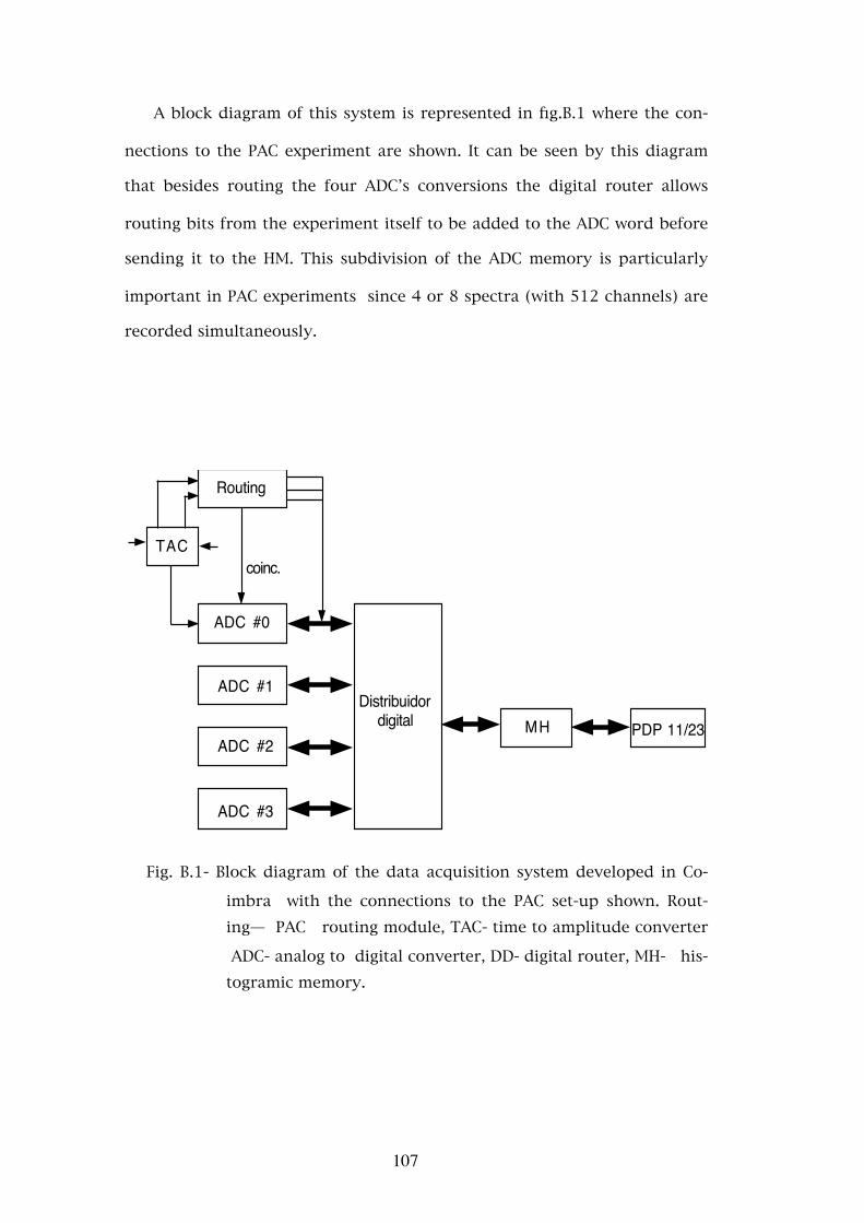
A block diagram of this system is represented in fig.B.1 where the con-

nections to the PAC experiment are shown. It can be seen by this diagram

that besides routing the four ADC’s conversions the digital router allows

routing bits from the experiment itself to be added to the ADC word before

sending it to the HM. This subdivision of the ADC memory is particularly

important in PAC experiments since 4 or 8 spectra (with 512 channels) are

recorded simultaneously.

coinc.

Routing

TAC

ADC #0

ADC #1

ADC #2

ADC #3

Distribuidordigital MH PDP 11/23

Fig. B.1- Block diagram of the data acquisition system developed in Co-

imbra with the connections to the PAC set-up shown. Rout-ing— PAC routing module, TAC- time to amplitude converter

ADC- analog to digital converter, DD- digital router, MH- his-togramic memory.

107

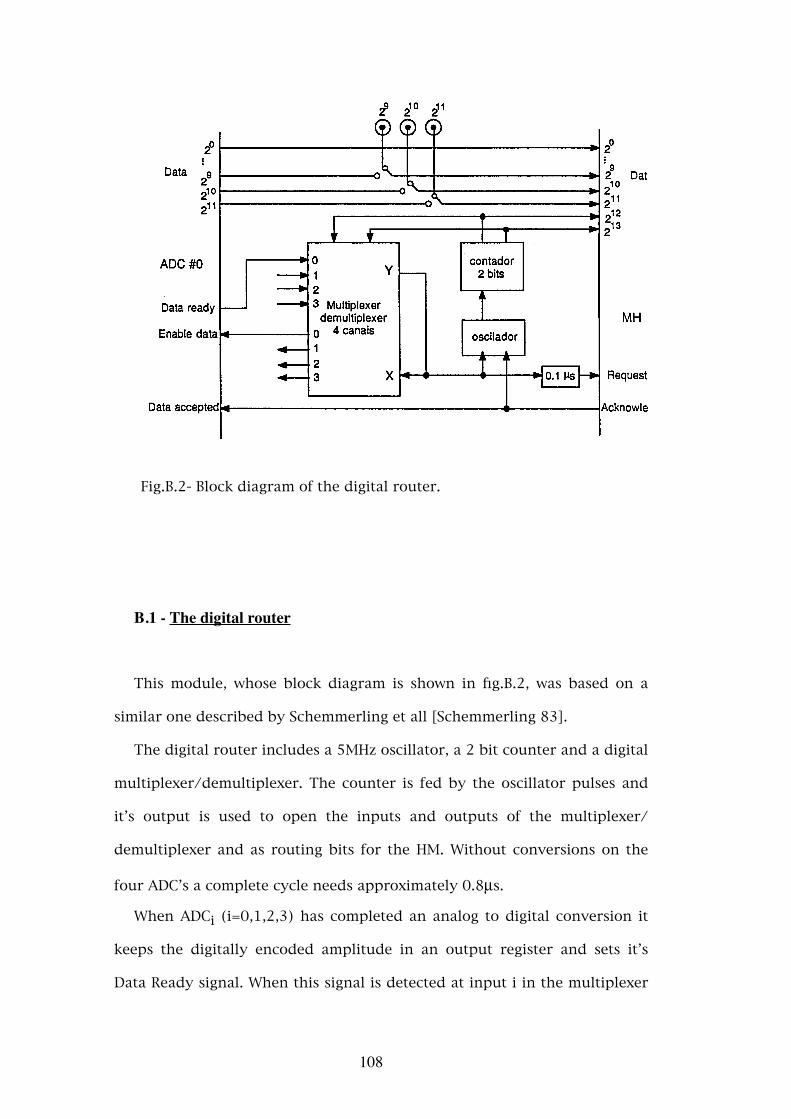
Fig.B.2- Block diagram of the digital router.

B.1 - The digital router

This module, whose block diagram is shown in fig.B.2, was based on a

similar one described by Schemmerling et all [Schemmerling 83].

The digital router includes a 5MHz oscillator, a 2 bit counter and a digital

multiplexer/demultiplexer. The counter is fed by the oscillator pulses and

it’s output is used to open the inputs and outputs of the multiplexer/

demultiplexer and as routing bits for the HM. Without conversions on the

four ADC’s a complete cycle needs approximately 0.8µs.

When ADCi (i=0,1,2,3) has completed an analog to digital conversion it

keeps the digitally encoded amplitude in an output register and sets it’s

Data Ready signal. When this signal is detected at input i in the multiplexer

108

it stops the oscillator via output Y. The same signal goes to input X of the

demultiplexer and is fed via it’s output i to the Enable Data of ADCi causing

it to send the output register contents to the address bus. The same Y signal,

after a delay of 0.1µs is sent to the Request input of the HM initiating a

Read-Increment cycle.

The HM receives 14 bits in it’s address bus. Bits 0 to 11 correspond to

the conversion of ADCi and bits 12 and 13 correspond to the counter

routing bits. After the Read-Increment cycle the HM sets it’s Acknowledge

signal which resets ADCi and disconnects it from the address bus. This sig-

nal also restarts the oscillator after the Y signal has disappeared.

109

REFERENCES

Arends 80 - A.R.Arends, C.Hohenemser, F.Pleiter, H.de Ward, L.Chow and R.M.Sutter, Hyp. Int. 8 (1980) 191-213

Baker 73 - C.Baker and H.K.Birnbaum, Acta Metall. 21 (1973) 865-871Bauer 75 - G.Bauer, E.Seitz, H.Horner and W.Schmtz, Sol.Stat. Comm. 17

(1975) 161-165Bevington 69 - P.R.Bevington, “Data Reduction and Error Analysis for the

Physical Sciences”, McGraw Hill Book Company, 1969, New York

Bodenstedt 85 - E.Bodensteadt, Hyp. Int. 24/26 (1985) 521-537Brigham 82 - E.O.Brigham, “FFT -Schnelle Fourier-Transformation”, R. Old-

enburg Verlag, 1982, MünchenCannelli 85 - G.Cannelli, R.Cantelli and F.Cordero, Phys. Rev. B32 (1985)

3573-3579Carstanjen 80 - H.D.Carstanjen, Phys. Stat. Sol. (a)59 (1980) 11-26

Carstanjen 82 - H.D.Carstanjen, Habilitation thesis, Universität München, 1982

Chen 76 - C.G.Chen and H.KBirnbaum, Phys. stat. sol. (a)36 (1976) 687-Christiansen 76 - J.Christiansen, P.Heubes, R.Keitel, W.Klinger, W.Loefler,

W.Sandner and W.Witthuhn, Z. Phys. B24 (1976) 177-187

Cost 84 - J.R.Cost, Acta Metall. 32 (1984) 123-130Cotton 66 - F.Cotton, G.Wilkinson, “Advanced Inorganic Chemistry”, John

Wiley & Sons, New York, 1966Dosch 85 - H.Dosch, U.Schubert, H.Metzger and J.Peisl, J. Phys. F14 (1984)

2467-2473Feiock 69 - F.D.Feiock and W.R.Johnson, Phys. Rev. 187 (1969)39-50

Forker 73 - M.Forker, Nucl. Instr. Meth. 106 (1973) 121-126Frauenfelder 65 - H.Frauenfelder and R.M.Steffen, in “Alpha-, Beta- and

Gamma-ray spectroscopy”, Vol 2, Cap.19, K.Siegbahn ed.,North-Holland Publ. Comp., Amesterdam, 1965

110

Fromm 80 - E.Fromm and G.Hörz, Int. Met. Rev. 5/6 (1980) 269-311

Gibala 85 - R.Gibala, J. Phys. Colloque C10-46 (1985) 43-46Gil 84 - J.M.Gil, P.J.Mendes, C.Lopes Gil, A.P.de Lima, N.Ayres deCampos and

A.Weidinger, J. Less Common Met. 103 (1984) 227-232Gil 87a - J.M.Gil, P.J.Mendes, A.P.de Lima, N.Ayres de Campos, S.Yuquin,

R.Peichl and A. Weidinger, J. Less Common Met. 129 (1987) 145-151

Gil 87b - J.M.Gil, Doctorate thesis, to be published

Hanada 77 - R.Hanada, Proc. 2nd Int. Conf. on Hydrogen in Metals, Paris, (Pergamon Oxford), Vol.3 (1977) 1B6

Hanada 81a - R.Hanada, M.Shinohara, Y.Sado and H.Kimura, J.Phys. Collo-

que C5 (1981) 757-761Hanada 81b - R.Hanada, Scripta Metall. 15 (1981) 1121-1125

Hiraga 77 - H.Hiraga, T.Onozuka and H.Hirabayashi, Mat. Sci. Eng. 27 (1977) 35-

Kaim 79 - R.E.Kaim and D.W.Palmer, Philos. Mag. A40 (1979) 279-296Kaufmann 79 - E.N.Kaufman and R.Vianden, Rev. Mod. Phys. 51 (1979)161-

214Lederer 78 - C.M.Lederer and V.S.Shirley eds., “Table of Isotopes”, 7ed., John

Wiley & Sons Inc., 1978, New YorkLocattelli 78 - M.Locattelli, K.Neumaier and H.Wipf, J. Phys. Colloque C6-39

(1985) 995-998Magerl 83 - A.Magerl, J.J.Rush, J.M.Rowe, D.Richter and H.Wipf, Phys Rev

B27 (1983) 927-934Magerl 86 - A.Magerl, J.Dianoux, H.Wipf, K.Neumaier and I.S.Anderson,

Phys. Rev. Lett. 56 (1986) 159-162Mattas 75 - R.F.Mattas and H.K.Birnbaum, Acta Metall. 23 (1975 973-977

Matthias 63 - E.Matthias, W.Schneider and R.M.Steffen, Phys. Lett. 4 (1963) 41-43

Mendes 83 - P.J.Mendes, J.M.Gil, N.Ayres de Campos, R.Peichl and A.Weidinger, Hyp.Int. 15/16 (1983) 791-794

Mendes 85 - P.J.Mendes, J.M.Gil, N.Ayres de Campos, A.Weidinger and R.Peichl, Zeit. Phys. Chem. Neue Folge 145 (1985) 141-

145Metzger 76 - H.Metzger, J.Peisl and J.Wanagel, J. Phys. F6 (1976) 2195-2206

Metzger 85 - H.Metzger, U.Schubert and J.Peisl, J. Phys. F15 (1985) 779-797

111

Moffat 78 - W.G.Moffat, “The Handbook of Binary Phase-Diagrams”, Genum

Publishing Company, New York, 1984Morkel 78 - C.Morkel, H.Wipf and K.Neumaier, Phys. Rev. Lett. 40 (1978)

947-950NDS 73 - Nuclear Data Sheets 9 (1973) 337

NDS 84 - Nuclear Data Sheets 43,3 (1984) 329Okuda 84 - S. Okuda, H. Mizubayashi, N. Martsumoto, N. Kuramochi, C. Mo-

chizuki and R. Hanada, Acta Metall. 32 (1984) 2125-2128

Nelson 75 - R.S.Nelson, “Radiation Damage Processes in Materials”, NATO Adv. Study Inst. Series E:Applied Sciences 8 (1975)

261-308Pal 85 - B.Pal, J.Singh, S.D.Raj and S.Prakash, Phys. Stat. Sol. (b)129 (1985)

301-312Peichl 83 - R.Peichl, A.Weidinger, E.Recknagel, J.M.Gil, P.J.Mendes and

N.Ayres de Campos, Hyp. Int. 15/16 (1983) 463-466Pfeiffer 76 - G.Pfeiffer and H.Wipf, J. Phys. F6 (1976) 167-179

Phillips 79 - M.E.Phillips and F.A.Smith, Nucl. Inst. Meth. 165 (1979) 83-90Pleiter 73 - F.Pleiter, H.Bertschat, E.Recknagel and B.Spelmeyer, Nucl. Phys.

A215 (1973) 471-476Poker 79 - D.B.Poker, G.G.Setser, A.V.Granato and H.KBirnbaum, Zeit. Phys.

Chem. Neue Folge 116 (1979) 39-45Poker 84 - D.B.Poker, G.G.Setser, A.V.Granato and H.KBirnbaum, Phys. Rev. B

29 (1984) 622-629Ponnambalam 84 - M.J.Ponnambalam and P.Jena, Hyp. Int. 20 (1984) 65-

117Ponnambalam 85 - M.J.Ponnambalam, J. Phys. F15 (1985) L7-L9

Prakash 85 - S.Prakash, Hyp.Int. 24-26 (1985) 491-519Qi 82 - Zh.Qi, J.Völkl and H.Wipf, Scr. Metall. 16 (1982) 859-864

Recknagel 83 - E.Recknagel, G.Schatz and Th.Wichert, “Hyperfine Interaction of Radioactive Nuclei”, Cap.4, J. Christiansen ed., Top-

ics in Current Physics, Springer Verlag, Berlin, 31 (1983) 133-204

Rosan 76 - K.Rosan and H.Wipf, Phys. Stat. Sol. (a)38 (1976) 611-620Rose 67 - H.J.Rose and D.M.Brink, Rev. Mod. Phys. 39 (1967) 306-347

Rowe 80 - J.M.Rowe and A.Magerl, Phys. Rev. B21 (1980) 1706-1707

112

Sado 82 - Y.Sado, M.Shinohara, R.Hanada and H.Kimura, Proc. 3rd. Int.

Congr. Hydr. in Mat., Paris, France, June 1982, pg.233-238

Schemmerling 83 - K.Schemmerling, J.Ahlert, M.Schumacher and F.Smend, Nucl. Instr. Meth. 216 (1983) 165-166

Schiller 75 - P.Schiller and H.Nijman, Phys.Stat. Sol. (a)31 (1975) K77-K79Schubert 84 - U.Schubert, H.Metzger and J.Peisl, J. Phys. F14 (1984) 2457-

2466Schulze 77 - K.Sculze and H.Jehn, Zeit. Metallkd. 68 (1977) 654-660

Schulze 79 - K.Sculze, H.Jehne and E.Grallath, Zeit. Metallkd. 70 (1979) 625-630

Shakun 85 - N.A.Shakun, P.A.Svetashov and V.E.Storizhko, Radiat. Effects 90 (1985) 49-56

Shirley 83 - A.I.Shirley, C.K.Hall and N.J.Prince, Acta Metall. 31 (1983) 985-992

Smithels 67 - C.J. Smithells, “Metals Referenca Book”, Butterworth & Co., London, 1967, Vol II, pg.628

Takahashi 78 - J. Takahashi, M.Koiwa, M.Hirabayashi, S.Yamaguchi, Y.Fujino, K.Ozawa and K.Doi, J. Phys. Soc. Jap. 45 (1978) 1690-

1696Taylor 67 - A.Taylor and N.J.Doyle, J. Less Common Met. 13 (1967) 313-330

Vianden 83 - R.Vianden, Hyp. Int. 15/16 (1983) 189-202Weidinger 79 - A.Weidinger, R.Wessner, Th.Wichert and E.Recknagel, Phys.

Lett. 72A (1979) 369-372Weidinger 81 - A.Weidinger, M.Deicher and T.Butz, Hyp. Int. 10 (1981) 717-

720Weidinger 85 - A.Weidinger and R.Peichl, Phys. Rev. Lett. 54 (1985) 1683-

1685Weller 85a - M.Weller, J. Phys. Colloque C10-46 (1985) 7-14

Weller 85b - M.Weller,I.Diehl, G.Hörz, R.Mann and K.Schulze, J. Phys. Collo-que C10-46 (1985) 47-50

Wipf 81 - H.Wipf, A.Magerl, S.M.Shapiro, S.K.Satija and W. Thomlinson, Phys. Rev. Lett. 46 (1981) 947-950

Wipf 82 - H.Wipf and K.Neumaier, Proc. Int. Symp. on the Electronic Struc-ture and Properties of Hydrogen in Metals, Richmond,

USA, 1982Wipf 84 - H.Wipf and K.Neumaier, Phys. Rev. Lett. 52 (1982) 1308-1311

113

Witthuhn 83 - W.Witthuhn and W Engel, “Hyperfine Interactions of Radioac-

tive Nuclei”, Cap.5, Topics in Current Physics, J.Christiansen ed., Springer Verlag, Berlin, 31 (1983)

205-289 Wrede 86 - U.Wrede, T.Schaefer and R.Vianden, Zeit. Phys. B64 (1986) 461-

467Yates 65 - M.J.L.Yates, in “Alpha-, Beta- and Gamma-ray spectroscopy”, Ap-

pendix 9, Vol 2, K.Siegbahn ed., North-Holland Publ. Comp., Amesterdam, 1965

Zapp 80a - P.E.Zapp and H.K.Birnbaum, Acta Metall. 28 (1980) 1275-1286Zapp 80b - P.E.Zapp and H.K.Birnbaum, Acta Metall. 28 (1980) 1523-1526

114