h. lu et al- stainless super p-branes
TRANSCRIPT
8/3/2019 H. Lu et al- Stainless Super p-branes
http://slidepdf.com/reader/full/h-lu-et-al-stainless-super-p-branes 1/35
a r X i v : h e p - t h / 9 5 0 8 0 4 2 v 2
1 2 O c t 9 5
CTP TAMU-31/95
Imperial/TP/94-95/56
SISSA 97/95/EP
hep-th/9508042
Stainless Super p-branes
H. Lu♣♥1, C.N. Pope♣♥1,2, E. Sezgin♣♠3 and K.S. Stelle♦♥4
♣ Center for Theoretical Physics, Texas A&M University, College Station, TX 77843-4242, USA
♦ The Blackett Laboratory, Imperial College, Prince Consort Road, London SW7 2BZ, UK
♥ SISSA, Via Beirut No. 2-4, 34013 Trieste, Italy
♠ ICTP, Strada Costiera 11, 34013 Trieste, Italy
Abstract
The elementary and solitonic supersymmetric p-brane solutions to supergravity theo-
ries form families related by dimensional reduction, each headed by a maximal (‘stainless’)
member that cannot be isotropically dimensionally oxidized into higher dimensions. We find
several new families, headed by stainless solutions in various dimensions D ≤ 9. In some
cases, these occur with dimensions (D, p) that coincide with those of descendants of known
families, but since the new solutions are stainless, they are necessarily distinct. The new
stainless supersymmetric solutions include a 6-brane and a 5-brane in D = 9, a string in
D = 5, and particles in all dimensions 5 ≤ D ≤ 9.
1Supported in part by the U.S. Department of Energy, under grant DE–FG05–91–ER40633.
2Supported in part by the EC Human Capital and Mobility Programme under contract ERBCHBGCT920176.
3Supported in part by the National Science Foundation, under grant PHY–9411543.
4Supported in part by the Commission of the European Communities under contract SC1*–CT92–0789.
8/3/2019 H. Lu et al- Stainless Super p-branes
http://slidepdf.com/reader/full/h-lu-et-al-stainless-super-p-branes 2/35
1 Introduction
Since the discovery of p-brane theories with manifest spacetime supersymmetry [1, 2], it has
become increasingly clear that there is a close relationship between such theories and the set of
soliton-like solutions to supergravity theories [3]. All the known supersymmetric p-brane theo-
ries achieve a matching of the on-shell world-volume bosonic and fermionic degrees of freedom,
by virtue of a local fermionic symmetry known as κ symmetry. This symmetry compensates
for the excess of fermionic over bosonic degrees of freedom by gauging away half of the former.
The consistency of κ symmetry with spacetime supersymmetry places severe constraints on the
spacetime dimension D and the world volume dimension d = p + 1 [4]. Four classic families of
super p-branes were found to satisfy the consistency criterion. The members within each family
are related by a process of double dimensional reduction [5], in which both the spacetime and
the world volume are simultaneously compactified on a circle, and the dependence on the extra
direction is dropped in each space. Thus the classic super p-branes may be classified by giving
the maximal-dimensional member of each of the four families. These occur in (D, d) = (11, 3),
(10, 6), (6, 4) and (4, 3). On a plot or ‘brane scan’ of D vs d, the additional p-branes obtained by
double dimensional reduction lie on the North-east/South-west diagonal lines descending from
the maximal cases.
The idea that a super p-brane could be viewed as a long-wavelength description of a topo-
logical defect in a supersymmetric theory originated in the construction of the supermembrane
in D = 4 [1]. This supermembrane occurs as a kink solution of a D = 4 chiral scalar supermul-
tiplet theory with a potential giving a degenerate vacuum. A crucial feature of this solution is
that half the original supersymmetry is left unbroken. This partial breaking of supersymmetry
is also a general feature of all the subsequently-discovered p-brane solitons.
Another feature of super p-branes became clear with the curved-superspace construction
of the D = 11 supermembrane action in [2], and its generalisations to the other classic super
p-branes. This new feature was the occurrence of integrability conditions on the supergravity
background that are required for the existence of the world-volume κ symmetry. In the case
of the D = 11 supermembrane, and of the type IIA string, related to it by double dimensional
reduction, these integrability conditions imply the full set of supergravity field equations [2, 5].
The association of super p-branes to supergravity is also natural because the supersymmetric
p-branes can be viewed as the natural ‘matter’ sources for the corresponding supergravity
theories. A very specific role in this association is played by the antisymmetric tensor field
1
8/3/2019 H. Lu et al- Stainless Super p-branes
http://slidepdf.com/reader/full/h-lu-et-al-stainless-super-p-branes 3/35
strengths, whose gauge potentials couple directly to the ( p + 1)-dimensional world volumes.
In the coupled solutions of super p-branes and their corresponding supergravity backgrounds,
the backgrounds are naturally singular on the p-brane world volumes, which can act like delta-
function sources. These singularities may or may not be clothed by horizons, depending upon
the circumstances. Such singular supergravity solutions are called ‘elementary,’ in distinction
to the non-singular ‘solitonic’ solutions described previously.
The association of p-branes with singular supergravity solutions was made concrete with
the explicit construction of superstring solutions in the case of N = 1, D = 10 supergravity [6].
These solutions preserve half of the original supersymmetry, and consequently they saturate a
Bogomol’ny bound on the energy density. Subsequently, an analogous elementary membrane
solution of D = 11 supergravity was found [7]. Many further solutions of supergravity theories
have also been found, both for elementary p-branes [8] and for solitonic p-branes [9]. (There
are also solitonic solutions in supergravity theories coupled to Yang-Mills, such as that based
upon Yang-Mills instantons, and corresponding to the heterotic string [10].)
The multiplicity of elementary and solitonic p-brane solutions to supergravity theories, cov-
ering many more values of (D, d) than the classic κ-symmetric points on the brane scan, suggests
that the original classification needs to be generalised. Leaving aside for the moment the prob-
lem of formulating more general κ-symmetric actions, it is worthwhile to try to find the general
pattern of elementary and solitonic p-brane solutions in supergravity theories.Many supergravity theories in D ≤ 10 dimensions can be obtained from D = 11 super-
gravity by Kaluza-Klein dimensional reduction, in which a consistent truncation of the higher-
dimensional to the lower-dimensional theory is made. Since the truncation is consistent, it fol-
lows that solutions of the lower-dimensional theory are also solutions of the higher-dimensional
one. This lifting of solutions to the higher dimension is known as dimensional oxidation. In
some cases, an elementary or solitonic brane solution in the lower dimension oxidizes to another
elementary or solitonic brane solution in the higher dimension. The ability to view an oxidized
brane solution as itself being a brane solution depends upon whether the isotropicity of thelower-dimensional solution extends to an isotropicity in the higher-dimensional sense. For the
isotropicity to extend, the extra coordinate of the higher-dimensional spacetime must either
become isotropically grouped with the p-brane coordinates of the lower dimension, making a
( p+1)-brane, or else it must become isotropically grouped with the coordinates of the transverse
space, making a p-brane in the higher dimension. As we shall show later, the latter can never
happen within the framework of Kaluza-Klein dimensional reduction. The former, on the other
2
8/3/2019 H. Lu et al- Stainless Super p-branes
http://slidepdf.com/reader/full/h-lu-et-al-stainless-super-p-branes 4/35
8/3/2019 H. Lu et al- Stainless Super p-branes
http://slidepdf.com/reader/full/h-lu-et-al-stainless-super-p-branes 5/35
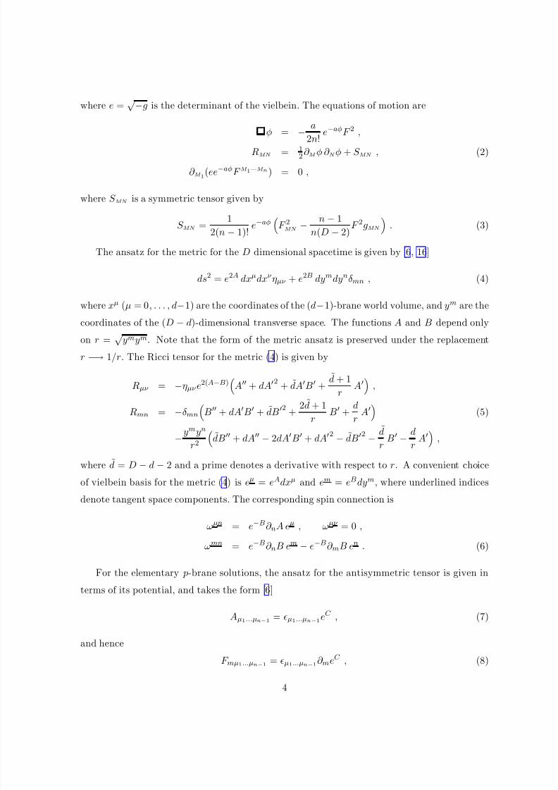
where e =√−g is the determinant of the vielbein. The equations of motion are
φ =−
a
2n!e−aφF 2 ,
RMN = 12∂ M φ ∂ N φ + S MN , (2)
∂ M 1(ee−aφF M 1···M n) = 0 ,
where S MN is a symmetric tensor given by
S MN =1
2(n − 1)!e−aφ
F 2MN −
n − 1
n(D − 2)F 2gMN
. (3)
The ansatz for the metric for the D dimensional spacetime is given by [6, 16]
ds2 = e2A dxµdxν ηµν + e2B dymdynδmn , (4)
where xµ (µ = 0, . . . , d−1) are the coordinates of the (d−1)-brane world volume, and ym are the
coordinates of the (D − d)-dimensional transverse space. The functions A and B depend only
on r =√
ymym. Note that the form of the metric ansatz is preserved under the replacement
r −→ 1/r. The Ricci tensor for the metric (4) is given by
Rµν = −ηµν e2(A−B)
A + dA2 + dAB +
d + 1
rA
,
Rmn = −δmnB + dAB +˜dB
2
+
2d + 1
r B +
d
r A (5)
−ymyn
r2
dB + dA − 2dAB + dA2 − dB2 − d
rB − d
rA
,
where d = D − d − 2 and a prime denotes a derivative with respect to r. A convenient choice
of vielbein basis for the metric (4) is eµ = eAdxµ and em = eBdym, where underlined indices
denote tangent space components. The corresponding spin connection is
ωµn = e−B∂ nA eµ , ωµν = 0 ,
ωmn = e−B∂ nB em
−e−B∂ mB en . (6)
For the elementary p-brane solutions, the ansatz for the antisymmetric tensor is given in
terms of its potential, and takes the form [6]
Aµ1...µn−1 = µ1...µn−1eC , (7)
and hence
F mµ1...µn−1 = µ1...µn−1∂ meC , (8)
4
8/3/2019 H. Lu et al- Stainless Super p-branes
http://slidepdf.com/reader/full/h-lu-et-al-stainless-super-p-branes 6/35
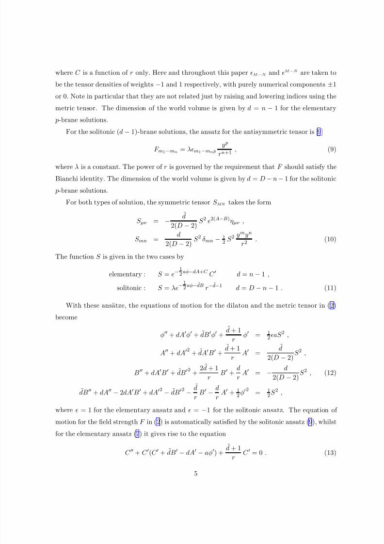
where C is a function of r only. Here and throughout this paper M ···N and M ···N are taken to
be the tensor densities of weights −1 and 1 respectively, with purely numerical components ±1
or 0. Note in particular that they are not related just by raising and lowering indices using the
metric tensor. The dimension of the world volume is given by d = n − 1 for the elementary
p-brane solutions.
For the solitonic (d − 1)-brane solutions, the ansatz for the antisymmetric tensor is [9]
F m1···mn = λm1···mn py p
rn+1, (9)
where λ is a constant. The power of r is governed by the requirement that F should satisfy the
Bianchi identity. The dimension of the world volume is given by d = D − n − 1 for the solitonic
p-brane solutions.
For both types of solution, the symmetric tensor S MN takes the form
S µν = − d
2(D − 2)S 2 e2(A−B)ηµν ,
S mn =d
2(D − 2)S 2 δmn − 1
2 S 2ymyn
r2. (10)
The function S is given in the two cases by
elementary : S = e−12aφ−dA+C C d = n − 1 ,
solitonic : S = λe−12aφ−dB r−d−1 d = D − n − 1 . (11)
With these ansatze, the equations of motion for the dilaton and the metric tensor in ( 2)
become
φ + dAφ + dBφ +d + 1
rφ = 1
2aS 2 ,
A + dA2 + dAB +d + 1
rA =
d
2(D − 2)S 2 ,
B + dAB + dB2 +2d + 1
rB +
d
rA =
−
d
2(D−
2)S 2 , (12)
dB + dA − 2dAB + dA2 − dB2 − d
rB − d
rA + 1
2φ2 = 12S 2 ,
where = 1 for the elementary ansatz and = −1 for the solitonic ansatz. The equation of
motion for the field strength F in (2) is automatically satisfied by the solitonic ansatz (9), whilst
for the elementary ansatz (7) it gives rise to the equation
C + C (C + dB − dA − aφ) +d + 1
rC = 0 . (13)
5
8/3/2019 H. Lu et al- Stainless Super p-branes
http://slidepdf.com/reader/full/h-lu-et-al-stainless-super-p-branes 7/35
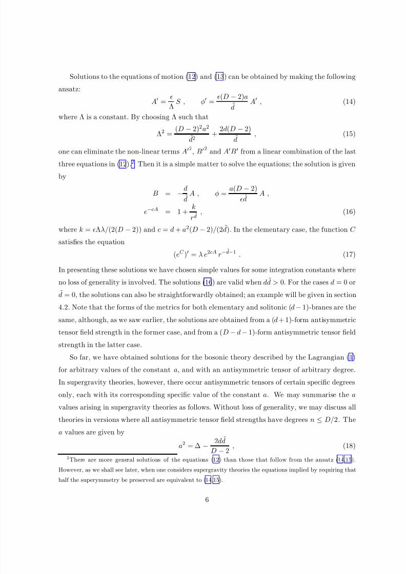
Solutions to the equations of motion (12) and (13) can be obtained by making the following
ansatz:
A = Λ S , φ = (D − 2)ad
A , (14)
where Λ is a constant. By choosing Λ such that
Λ2 =(D − 2)2a2
d2+
2d(D − 2)
d, (15)
one can eliminate the non-linear terms A2, B2 and AB from a linear combination of the last
three equations in (12).2 Then it is a simple matter to solve the equations; the solution is given
by
B =
−
d
d
A , φ =a(D − 2)
d
A ,
e−cA = 1 +k
rd, (16)
where k = Λλ/(2(D − 2)) and c = d + a2(D − 2)/(2d). In the elementary case, the function C
satisfies the equation
(eC ) = λ e2cA r−d−1 . (17)
In presenting these solutions we have chosen simple values for some integration constants where
no loss of generality is involved. The solutions (16) are valid when dd > 0. For the cases d = 0 or
d = 0, the solutions can also be straightforwardly obtained; an example will be given in section
4.2. Note that the forms of the metrics for both elementary and solitonic (d − 1)-branes are the
same, although, as we saw earlier, the solutions are obtained from a (d + 1)-form antisymmetric
tensor field strength in the former case, and from a (D − d − 1)-form antisymmetric tensor field
strength in the latter case.
So far, we have obtained solutions for the bosonic theory described by the Lagrangian (1)
for arbitrary values of the constant a, and with an antisymmetric tensor of arbitrary degree.
In supergravity theories, however, there occur antisymmetric tensors of certain specific degrees
only, each with its corresponding specific value of the constant a. We may summarise the a
values arising in supergravity theories as follows. Without loss of generality, we may discuss all
theories in versions where all antisymmetric tensor field strengths have degrees n ≤ D/2. The
a values are given by
a2 = ∆ − 2dd
D − 2, (18)
2There are more general solutions of the equations (12) than those that follow from the ansatz (14,15).
However, as we shall see later, when one considers supergravity theories the equations implied by requiring that
half the superymmetry be preserved are equivalent to (14,15).
6
8/3/2019 H. Lu et al- Stainless Super p-branes
http://slidepdf.com/reader/full/h-lu-et-al-stainless-super-p-branes 8/35
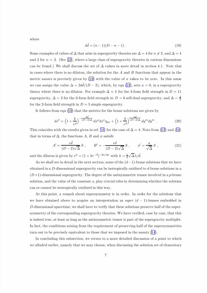
where
dd = (n − 1)(D − n − 1) . (19)
Some examples of values of ∆ that arise in supergravity theories are ∆ = 4 for n = 2, and ∆ = 4
and 2 for n = 2. (See [21], where a large class of supergravity theories in various dimensions
can be found.) We shall discuss the set of ∆ values in more detail in section 4.1. Note that
in cases where there is no dilaton, the solution for the A and B functions that appear in the
metric ansatz is precisely given by (16) with the value of a taken to be zero. In this sense
we can assign the value ∆ = 2dd/(D − 2), which, by eqn (18), sets a = 0, in a supergravity
theory where there is no dilaton. For example ∆ = 4 for the 4-form field strength in D = 11
supergravity, ∆ = 2 for the 3-form field strength in D = 6 self-dual supergravity, and ∆ = 43
for the 2-form field strength in D = 5 simple supergravity.
It follows from eqn (16) that the metrics for the brane solutions are given by
ds2 =
1 +k
rd
− 4d(D−2)∆ dxµdxν ηµν +
1 +
k
rd
4d(D−2)∆ dymdym . (20)
This coincides with the results given in ref. [16] for the case of ∆ = 4. Note from (15) and (16)
that in terms of ∆, the functions A, B and φ satisfy
A =d
(D − 2)√
∆S , B = − d
(D − 2)√
∆S , φ =
a√∆
S , (21)
and the dilaton is given by eφ = (1 + kr−d)−2a/∆ with k = 12√∆λ/d.
As we shall see in detail in the next section, some of the (d−1)-brane solutions that we have
obtained in a D-dimensional supergravity can be isotropically oxidized to d-brane solutions in a
(D +1)-dimensional supergravity. The degree of the antisymmetric tensor involved in a p-brane
solution, and the value of the constant a, play crucial roles in determining whether the solution
can or cannot be isotropically oxidized in this way.
At this point, a remark about supersymmetry is in order. In order for the solutions that
we have obtained above to acquire an interpretation as super (d − 1)-branes embedded in
D-dimensional spacetime, we shall have to verify that these solutions preserve half of the super-
symmetry of the corresponding supergravity theories. We have verified, case by case, that this
is indeed true, at least as long as the antisymmetric tensor is part of the supergravity multiplet.
In fact, the conditions arising from the requirement of preserving half of the supersymmetries
turn out to be precisely equivalent to those that we imposed in the ansatz ( 14).
In concluding this subsection, we return to a more detailed discussion of a point to which
we alluded earlier, namely that we may choose, when discussing the solution set of elementary
7
8/3/2019 H. Lu et al- Stainless Super p-branes
http://slidepdf.com/reader/full/h-lu-et-al-stainless-super-p-branes 9/35
and solitonic branes in supergravity theories, to restrict our attention to the versions of the
various supergravity theories in which all antisymmetric tensors F n have degrees n that do not
exceed D/2. The reason why we may do this without losing generality is that an elementary
or solitonic solution of a version of a supergravity theory in which the antisymmetric tensor
participating in the solution is dualised is precisely the same as the solitonic or elementary
solution, respectively, of the undualised form of the supergravity theory. To see this, consider
the solitonic solution of (2), with F n given by the ansatz (9). This has
F n =1
n!F m1···mn dym1 ∧ · · · ∧ dymn =
λ
n!e−nB m1···mn p
y p
rn+1em1 ∧ · · · ∧ emn . (22)
Thus the Hodge dual of this n-form is given by
∗ F n = λ(D − n)!
ym
rn+1e−nB µ1···µd em ∧ eµ1 ∧ · · · ∧ eµd . (23)
In the dual version of the theory, the (D − n)-form F whose Bianchi identity implies the field
equation for F n given in (2) is F = e−aφ ∗ F n, which, from (23), has components given by
F mµ1···µd =λym
rn+1edA−dB−aφ µ1···µd . (24)
Hence by using (16), with d = n − 1, we see that F mµ1···µd is precisely of the form of the
elementary ansatz (7) for a (d + 1)-index field strength, where the function C satisfies its
equation of motion (17). Thus we see that the solitonic solution of the dualised theory is
precisely the same thing as the elementary solution of the undualised theory, and vice versa ,
with the antisymmetric tensor written in different variables. We may therefore, without loss
of generality, consider all supergravity theories in their versions where the degrees of their
antisymmetric tensors F n satisfy n ≤ D/2. The set of all elementary and solitonic brane
solutions of these theories spans the entire set of inequivalent brane solutions of these theories
together with their dualised versions.
2.2 Kaluza-Klein dimensional reduction
In order to describe the processes of oxidation and reduction, we need to set up the Kaluza-
Klein procedure for dimensional reduction from (D + 1) to D dimensions. Let us denote the
coordinates of a (D + 1)-dimensional spacetime by xM = (xM , z), where z is the coordinate of
the extra dimension. The (D +1)-dimensional metric ds2 is related to the D-dimensional metric
ds2 by
ds2 = e2αϕds2 + e2βϕ(dz + AM dxM )2 , (25)
8
8/3/2019 H. Lu et al- Stainless Super p-branes
http://slidepdf.com/reader/full/h-lu-et-al-stainless-super-p-branes 10/35
where ϕ and A are taken to be independent of the extra coordinate z. The constants α and β
will be determined shortly. A convenient choice for the vielbein eAM of the (D + 1)-dimensional
spacetime is
eAM = eαϕ eAM , ezM = eβϕ AM ,
eAz = 0 , ezz = eβϕ . (26)
Note that M and z denote world indices, whilst A and z denote tangent-space indices.
The spin connection is given by
ωAB = ωAB + αe−αϕ
∂ Bϕ eA − ∂ Aϕ eB
− 12F ABe(β −2α)ϕ ez ,
ωAz =−
βe−αϕ ∂ Aϕ ez
−1
2F AB e(β −2α)ϕ eB , (27)
where ∂ A = E AM ∂ M is the partial derivative with a tangent-space index, and F MN = 2∂ [M AN ].
Here, E AM is the inverse vielbein in D dimensions. Choosing β = −(D − 2)α, we find that the
(D + 1)-dimensional Einstein-Hilbert action e R reduces to
eR = eR − (D − 1)(D − 2)α2 e(∂ϕ)2 − 14e e−2(D−1)αϕ F 2 . (28)
The Kaluza-Klein dilaton ϕ may be given its canonical normalisation by choosing the constant
α such that
α
2
=
1
2(D − 1)(D − 2) . (29)It is sometimes useful to have expressions for the (D + 1)-dimensional Ricci tensor. Its tangent-
space components are given, after setting β = −(D − 2)α, by
RAB = e−2αϕ
RAB − (D − 1)(D − 2)α2 ∂ Aϕ ∂ Bϕ − α ϕ ηAB
− 12e−2Dαϕ F ACF BC ,
RAz = 12e(D−3)αϕ B
e−2(D−1)αϕ F AB
, (30)
Rzz = (D − 2) α e−2αϕ ϕ + 14e−2Dαϕ F 2 .
Let us now apply the above formalism to the case of a bosonic Lagrangian of the form (1),
but in (D + 1) rather than D dimensions:
L = eR − 12 e(∂ φ)2 − 1
2 n!ee−aφ F 2n , (31)
where we add a subscript index n to indicate that F is an n-form. The Kaluza-Klein ansatz for
φ is simply φ = φ, where φ is independent of the extra coordinate z. For F n, which is written
locally in terms of a potential An−1 as F n = dAn−1, the ansatz for An−1 is
An−1 = Bn−1 + Bn−2 ∧ dz , (32)
9
8/3/2019 H. Lu et al- Stainless Super p-branes
http://slidepdf.com/reader/full/h-lu-et-al-stainless-super-p-branes 11/35
where Bn−1 and Bn−2 are potentials for the n-form field strength Gn = dBn−1 and the (n − 1)-
form field strength Gn−1 = dBn−2 in D dimensions. Defining
Gn = Gn − Gn−1 ∧ A , (33)
where A = AM dxM , one finds
F n = Gn + Gn−1 ∧ (dz + A) . (34)
The tangent-space components of F n in (D + 1) dimensions are therefore given by F A1···An =
GA1···Ane−nαϕ and F A1···An−1z = GA1···An−1e−(n−1)αϕ−βϕ . Substituting into (31), and using
β =
−(D
−2)α, we obtain the reduced D-dimensional Lagrangian
L = eR − 12e(∂φ)2 − 1
2e(∂ϕ)2 − 14ee−2(D−1)αϕ F 2
− e
2 n!e−2(n−1)αϕ−aφ G2
n − e
2 (n − 1)!e2(D−n)αϕ−aφ G2
n−1 , (35)
where α is given by (29). As one sees, different combinations of ϕ and φ appear in the expo-
nential prefactors of G2n and G2
n−1. Nonetheless, each of these prefactors may easily be seen to
be of the form e−anφ, where φ is an SO(2) rotated combination of ϕ and φ. In these prefactors,
the coefficients an satisfy the formula (18) in D dimensions, with dd given by (19), and with
the same value of ∆ as for a in (D + 1) dimensions. (Note that dd in (18) is n-dependent, so
one obtains different values for the G2n and G2
n−1 prefactors.) The 2-form field strength F has
an a value given by (18) with ∆ = 4.
Most supergravity theories can be obtained from 11-dimensional supergravity via Kaluza-
Klein dimensional reduction. Any such dimensional reduction can b e viewed as a sequence of
reductions by one dimension at a time, of the kind we are discussing here. Any solution of a
lower-dimensional supergravity theory in such a sequence can therefore be reinterpreted as a
solution of any one of the higher theories in the sequence by use of the Kaluza-Klein ansatz
(25). In particular, this implies that any elementary or solitonic p-brane solution is also a
solution in the higher dimensions. However, it is important to realise that the resulting higher
dimensional solution may not necessarily preserve the isotropic form of the p-brane ansatz (4).
In this paper, we are using the term ‘stainless’ to describe the property of a brane solution of
a lower-dimensional supergravity that cannot be oxidized into an isotropic brane solution in
any supergravity in the next higher dimension.3 On the other hand, a ( p + 1)-brane solution
3We note that in defining a stainless p-brane to be one that cannot be oxidized to an isotropic brane in a
10
8/3/2019 H. Lu et al- Stainless Super p-branes
http://slidepdf.com/reader/full/h-lu-et-al-stainless-super-p-branes 12/35
in (D + 1) dimensions necessarily gives rise under dimensional reduction to an isotropic p-
brane solution in D dimensions. This automatic preservation of isotropicity for solutions under
dimensional reduction corresponds directly to the process of double dimensional reduction [5]
of p-brane actions.
The above ideas can be illustrated in our example of the bosonic Lagrangians (31) and (35).
First, we shall show that the elementary and solitonic solutions in (D + 1) dimensions reduce
respectively to elementary and solitonic solutions in D dimensions. In the case of an elementary
solution, the n-index antisymmetric tensor in (D + 1) dimensions leads to an elementary brane
with world volume dimension d = n − 1. The elementary ansatz for the (D + 1)-dimensional
field strength F n in (31) is F mµ1...µn−2z = µ1...µn−2z∂ meC . It follows from eqn (34) that the
corresponding D dimensional fields Gn−1, Gn and A become
Gmµ1...µn−2 = µ1...µn−2∂ meC ,
GM 1...M n = 0 , AM = 0 . (36)
This is nothing but the usual elementary-type ansatz for an (n − 1)-index antisymmetric tensor
in D dimensions, and thus gives rise to an elementary brane solution (16) with world volume
dimension d = n − 2.
The metric ansatz in (D + 1) dimensions is given by ds2 = e2A(dxµdxν ηµν + dz2) +
e2Bdymdym. In the elementary solution in (D + 1) dimensions, it follows from (16) that
φ = a(D − 1)A/d, and B = −(d + 1)A/d. (Note that d is the same for both D and (D + 1)
dimensions since, by definition, d + 2 is the codimension of the world volume of the brane.)
On the other hand in D dimensions, we see from (35) that the combination of scalar fields
−2(D − n)αϕ + aφ = aφ, with a2 = a2 + 4(D − n)2α2, defines the SO(2)-rotated D-dimensional
dilaton φ, whilst the orthogonal combination 2(D − n)αφ + aϕ is set to zero. Since n = d + 2,
it then follows from (29) that a and a are related by
a2
= a2
−2d2
(D − 2)(D − 1) . (37)
higher dimension, we have not wanted to prejudge what a non-stainless p-brane may oxidize into. A priori , one
could envisage that the extra dimension acquired upon oxidation could either become isotropically included into
the world-brane dimensions, giving a ( p + 1)-brane in (D + 1) dimensions, or that the extra dimension could be
isotropically included into the transverse dimensions, in which case one would still have a p-brane in the (D + 1)
dimensions. The latter possibility, however, can never be realised within the scheme of Kaluza-Klein dimensional
reduction because all fields are by construction taken to be independent of the extra coordinate, and this would
be inconsistent with our ansatz (4).
11
8/3/2019 H. Lu et al- Stainless Super p-branes
http://slidepdf.com/reader/full/h-lu-et-al-stainless-super-p-branes 13/35
Thus we find that φ = a(D − 2)A/d, B = −dA/d and ecA = ecA, since, from the Kaluza-Klein
ansatz (25) for the metric, we have A = A + αϕ and B = B + αϕ. But these expressions for φ
and B are precisely of the form given in (16) for the elementary (d − 1)-brane in D dimensions.
Thus we conclude that under dimensional reduction, an elementary d-brane in (D + 1) reduces
to an elementary (d − 1)-brane in D dimensions.
In the case of solitonic solutions, the analysis is parallel. The ansatz for the n-index antisym-
metric tensor, which leads to a solitonic brane solution with world volume dimension d = D −n
in (D + 1) dimensions, takes the form F m1...mn = λm1...mn p y p r−n−1. It follows from eqn (34)
that the corresponding D dimensional fields Gn, Gn−1 and A become
Gm1...mn = λm1...mn p y p r−n−1 ,
GM 1...M n−1 = 0 , AM = 0 . (38)
This is indeed just the field configuration for a solitonic (d − 1)-brane in D dimensions. The
analysis of the relation between the metrics in (D +1) and D dimensions is very similar to that
in the elementary case.
It is of interest to note that in the reduction of a d-brane in (D + 1) dimensions to a (d − 1)
brane in D dimensions, the degree of the antisymmetric tensor involved in the solution reduces
by one in the elementary case, but remains unchanged in the solitonic case. Note also that the
relation between a and a in eqn (37) is always satisfied in the dimensional reduction of a brane
solution in (D +1) to one in D dimensions. This implies, conversely, that eqn (37) is a necessary
condition for the reverse procedure to be possible. It is easy to verify that the relation ( 37) is
uniquely satisfied with a and a given by eqn (18), provided that ∆ is the same for both a and
a.
We have seen that brane solutions in higher dimensions can be reduced to those in lower
dimensions via the Kaluza-Klein procedure; however, the inverse procedure is not necessarily
possible. For example the D-dimensional bosonic Lagrangian (35) that is derived from the
(D + 1)-dimensional Lagrangian (31) admits six brane solutions, namely an elementary and a
solitonic solution for each of the three antisymmetric tensors Gn, Gn−1 and F . Two of these
solutions are isotropically oxidizable to brane solutions in (D + 1) dimensions, by reversing
the procedure discussed above, namely the elementary solution using Gn−1 and the solitonic
solution using Gn. The remaining four solutions are stainless because they cannot be oxidized to
isotropic brane solutions of the (D+1) dimensional theory defined by eqn (31). To illustrate this,
consider the elementary solution that uses the antisymmetric tensor Gn in the D-dimensional
12
8/3/2019 H. Lu et al- Stainless Super p-branes
http://slidepdf.com/reader/full/h-lu-et-al-stainless-super-p-branes 14/35
Lagrangian (35). The solution for the metric in D dimensions is given by (4) with A and B
given in eqn (16). This solution can be oxidized into a solution in (D + 1) dimensions, whose
metric is given by
ds2 = e2Adxµdxν ηµν + e2B(dymdym + dz2) , (39)
where
A =(D − 2)(d + 1)
(D − 1)dA , B = − (D − 2)d
(D − 1)dA . (40)
From the form of this (D+1)-dimensional metric, we can see that it does not describe an isotropic
d-brane, since the different r-dependent prefactor for dz2 prevents z from being grouped together
with the coordinates xµ. Note also that, although dz2 does have the same prefactor as dymdym,
this metric is still not isotropic in the transverse directions because the prefactors e2A
and e2B
are functions of r =√
ymym and not of
ymym + z2.
To summarise, we have seen that an elementary or solitonic ( p +1)-brane solution in (D + 1)
dimensions can always be reduced respectively to an elementary or solitonic p-brane solution in
D dimensions. On the other hand, the inverse process of dimensional oxidation to an isotropic
brane solution is not always possible. Thus in a brane scan of elementary and solitonic solutions,
we may factor out the rusty solutions and characterise the full solution set by the stainless p-
branes only.
There are three cases in which a p-brane solution can turn out to be stainless. The first caseis when a brane solution arises in a supergravity theory that cannot be obtained by dimensional
reduction, such as D = 11 supergravity or type IIB supergravity in D = 10. In the remaining
two cases, the supergravity theory itself can be obtained by dimensional reduction, but oxidation
to an isotropic brane solution is nonetheless not possible. In the second case, no (D + 1)-
dimensional supergravity theory has the necessary antisymmetric tensor for an isotropic brane
solution. Specifically, if the D-dimensional solution is elementary, the (D+1)-dimensional theory
would need an antisymmetric tensor of degree one higher than that in the D-dimensional theory.
If it is instead a solitonic solution, the (D +1)-dimensional theory would need an antisymmetrictensor of the same degree as in the D-dimensional theory. In the third case, an antisymmetric
tensor of the required degree exists in the (D + 1)-dimensional theory, but the exponential
dilaton prefactor has a coefficient a that does not satisfy eqn (37). We shall meet examples of
all three cases in the subsequent sections.
13
8/3/2019 H. Lu et al- Stainless Super p-branes
http://slidepdf.com/reader/full/h-lu-et-al-stainless-super-p-branes 15/35
3 D ≥ 10 supergravity
D = 11 is the highest dimension for any supergravity theory, and hence all the D = 11 p-brane
solutions are necessarily stainless. Since there is only one antisymmetric tensor field strength in
the theory, namely a 4-index field, there is just one elementary membrane solution [7] and one
solitonic 5-brane solution [11]. (Original papers giving D = 11 supergravity, and all the other
supergravities in various dimensions that we will consider here, can be found in [ 21].)
Dimensional reduction of D = 11 supergravity to D = 10 yields type IIA supergravity. The
type IIA theory contains: a 2-form field strength giving rise to a particle and a 6-brane; a 3-form
giving rise to a string and a 5-brane; and a 4-form giving rise to a membrane and a 4-brane.
In each case we have listed first the elementary and then the solitonic solution. All of these
solutions break half of the D = 10, N = 2 supersymmetry. Of the six solutions two, namely the
elementary string and the solitonic 4-brane, can be oxidized to the corresponding elementary
membrane and solitonic 5-brane in D = 11. The remaining four solutions are stainless since
D = 11 supergravity lacks the necessary antisymmetric tensors. Note that the 11 −→ 10
situation corresponds precisely to the bosonic example we discussed in section 2.2.
In addition, in D = 10, there is the type IIB supergravity, which cannot be obtained by
dimensional reduction from D = 11. This theory contains a complex 3-form field strength giving
rise to an elementary string and a solitonic 5-brane solution; and a self-dual 5-form field strength
giving rise to a self-dual 3-brane [12]. The string and 5-brane are in fact also solutions of D = 10,
N = 1 supergravity, and are hence identical to the string and 5-brane solutions of the type IIA
theory. Thus, although the type IIB theory cannot itself be obtained by dimensional reduction
from D = 11, these particular solutions of the IIB theory do have an oxidation pathway up
to isotropic solutions in D = 11. In such situations, we do not consider brane solutions to
be stainless. The remaining solution, the self-dual 3-brane, is the only solution that belongs
exclusively to the IIB theory. It is stainless and breaks half of the N = 2 supersymmetry.
4 D = 9 supergravity
4.1 N = 1, D = 9 supergravity
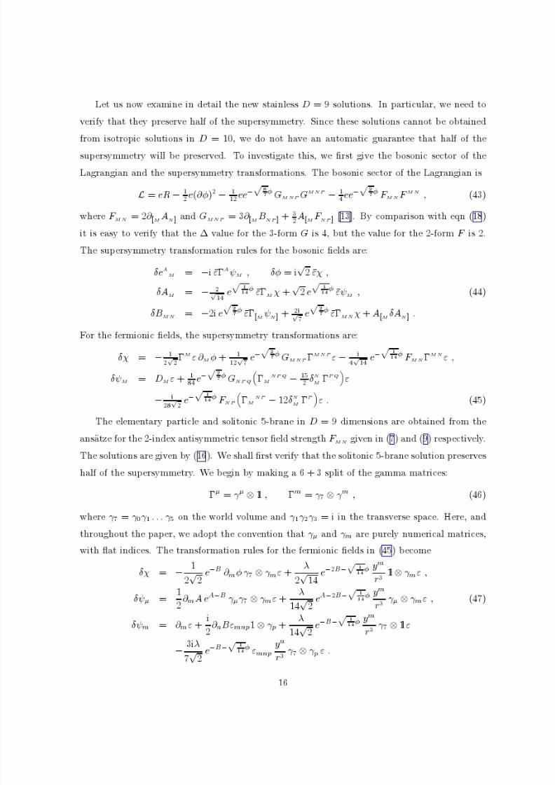
N = 1 supergravity in D = 9 [13] contains a 2-form field strength giving rise to an elementary
particle and a solitonic 5-brane; and a 3-form field strength giving rise to an elementary string
and a solitonic 4-brane. The solitonic 4-brane solution can be isotropically oxidized to the
14
8/3/2019 H. Lu et al- Stainless Super p-branes
http://slidepdf.com/reader/full/h-lu-et-al-stainless-super-p-branes 16/35
solitonic 5-brane of N = 1, D = 10 supergravity. The situation is somewhat more complicated
for the oxidation of the elementary string solution. Obviously, this solution cannot be oxidized
isotropically to an elementary membrane solution of N = 1, D = 10 supergravity because this
theory lacks the necessary 4-form field strength, and thus no elementary membrane exists in
the N = 1, D = 10 theory. Nonetheless, the D = 9 string solution is not stainless because
there is a different oxidation pathway available to it. The D = 9 string can also be viewed as a
solution of N = 2, D = 9 supergravity. In this guise, it can oxidize isotropically to a solution
of type IIA D = 10 supergravity, which does have a 4-form field strength.
The elementary particle and solitonic 5-brane solution that arise from the 2-form field
strength are stainless. Naıvely, one might expect these solutions could oxidize up to the el-
ementary string and solitonic 6-brane solutions of type IIA D = 10 supergravity. However, as
we showed in section 2.2, even when the necessary forms are present in the higher-dimensional
theory an isotropic oxidation is possible only when the coefficient a appearing in the dilaton
prefactor e−aφ satisfies the relation (37). In the case of N = 1, D = 9 supergravity, the coeffi-
cient a is given by eqn (18) with ∆ = 2. On the other hand, the coefficient a in the type IIA,
D = 10 theory is given by eqn (18) with ∆ = 4. Since the ∆ value has to be preserved under
dimensional reduction, it follows that the particle and 5-brane solutions in D = 9 are stainless.
There are elementary particle and solitonic 5-brane descendants in D = 9, nonetheless.
These are obtained by dimensional reduction from the type IIA D = 10 elementary membraneand solitonic 6-brane. From the D = 9 point of view, these are obtained as solutions to N = 2
supergravity using a 2-form field strength whose dilaton prefactor indeed has an a coefficient
given by (18) with the necessary ∆ = 4. The difference in ∆ values establishes the distinctness of
the stainless particle and 5-brane discussed above from those obtained by dimensional reduction.
The metrics for the stainless elementary particle and solitonic 5-brane are given by
elementary : ds2 = −
1 +k
r6
−12/7dt2 +
1 +
k
r6
2/7dymdym ,
solitonic : ds2
= 1 +
k
r −2/7
dxµ
dxν
ηµν + 1 +
k
r 12/7
dym
dym
. (41)
By contrast, the metrics for the elementary particle and solitonic 5-brane that can oxidize to
an elementary string and a solitonic 6-brane in D = 10 are given by
elementary : ds2 = −
1 +k
r6
−6/7dt2 +
1 +
k
r6
1/7dymdym ,
solitonic : ds2 =
1 +k
r
−1/7dxµdxν ηµν +
1 +
k
r
6/7dymdym . (42)
15
8/3/2019 H. Lu et al- Stainless Super p-branes
http://slidepdf.com/reader/full/h-lu-et-al-stainless-super-p-branes 17/35
8/3/2019 H. Lu et al- Stainless Super p-branes
http://slidepdf.com/reader/full/h-lu-et-al-stainless-super-p-branes 18/35
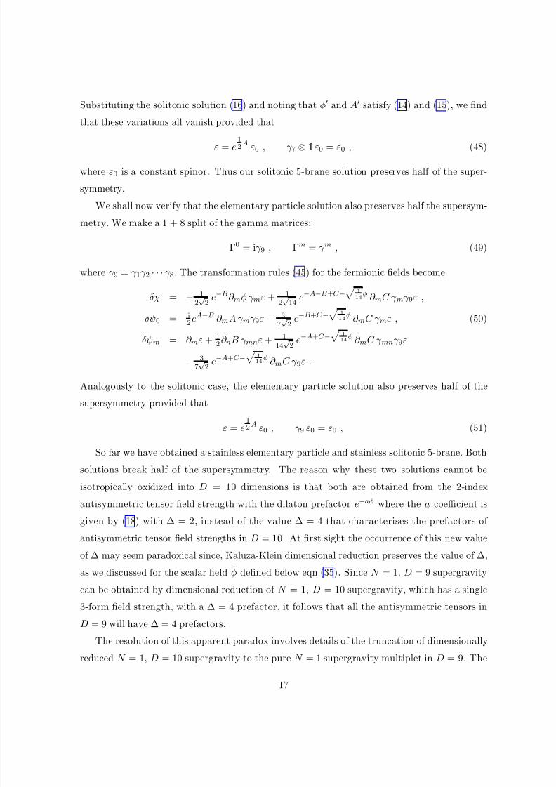
Substituting the solitonic solution (16) and noting that φ and A satisfy (14) and (15), we find
that these variations all vanish provided that
ε = e12A ε0 , γ 7 ⊗ 1l ε0 = ε0 , (48)
where ε0 is a constant spinor. Thus our solitonic 5-brane solution preserves half of the super-
symmetry.
We shall now verify that the elementary particle solution also preserves half the supersym-
metry. We make a 1 + 8 split of the gamma matrices:
Γ0 = iγ 9 , Γm = γ m , (49)
where γ 9 = γ 1γ 2 · · · γ 8. The transformation rules (45) for the fermionic fields become
δχ = − 12√2
e−B∂ mφ γ mε + 12√14
e−A−B+C −
1
14φ ∂ mC γ mγ 9ε ,
δψ0 = i2eA−B ∂ mA γ mγ 9ε − 3i
7√2
e−B+C −
1
14φ ∂ mC γ mε , (50)
δψm = ∂ mε + i2∂ nB γ mnε + 1
14√2
e−A+C −
1
14φ ∂ mC γ mnγ 9ε
− 37√2
e−A+C −
1
14φ ∂ mC γ 9ε .
Analogously to the solitonic case, the elementary particle solution also preserves half of the
supersymmetry provided that
ε = e12A ε0 , γ 9 ε0 = ε0 , (51)
So far we have obtained a stainless elementary particle and stainless solitonic 5-brane. Both
solutions break half of the supersymmetry. The reason why these two solutions cannot be
isotropically oxidized into D = 10 dimensions is that both are obtained from the 2-index
antisymmetric tensor field strength with the dilaton prefactor e−aφ where the a coefficient is
given by (18) with ∆ = 2, instead of the value ∆ = 4 that characterises the prefactors of
antisymmetric tensor field strengths in D = 10. At first sight the occurrence of this new value
of ∆ may seem paradoxical since, Kaluza-Klein dimensional reduction preserves the value of ∆,
as we discussed for the scalar field φ defined below eqn (35). Since N = 1, D = 9 supergravity
can be obtained by dimensional reduction of N = 1, D = 10 supergravity, which has a single
3-form field strength, with a ∆ = 4 prefactor, it follows that all the antisymmetric tensors in
D = 9 will have ∆ = 4 prefactors.
The resolution of this apparent paradox involves details of the truncation of dimensionally
reduced N = 1, D = 10 supergravity to the pure N = 1 supergravity multiplet in D = 9. The
17
8/3/2019 H. Lu et al- Stainless Super p-branes
http://slidepdf.com/reader/full/h-lu-et-al-stainless-super-p-branes 19/35
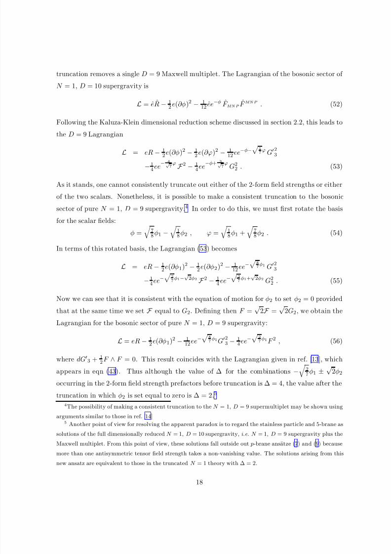
truncation removes a single D = 9 Maxwell multiplet. The Lagrangian of the bosonic sector of
N = 1, D = 10 supergravity is
L = eR − 12e(∂φ)2 − 1
12 ee−φ F MNP F MNP . (52)
Following the Kaluza-Klein dimensional reduction scheme discussed in section 2.2, this leads to
the D = 9 Lagrangian
L = eR − 12e(∂φ)2 − 1
2e(∂ϕ)2 − 112ee−φ−
1
7ϕ G2
3
−14ee
− 4√ 7ϕ F 2 − 1
4ee−φ+ 3√
7ϕ
G22 . (53)
As it stands, one cannot consistently truncate out either of the 2-form field strengths or either
of the two scalars. Nonetheless, it is possible to make a consistent truncation to the bosonic
sector of pure N = 1, D = 9 supergravity.4 In order to do this, we must first rotate the basis
for the scalar fields:
φ =
78φ1 −
18φ2 , ϕ =
18φ1 +
78φ2 . (54)
In terms of this rotated basis, the Lagrangian (53) becomes
L = eR − 12e(∂φ1)2 − 1
2e(∂φ2)2 − 112ee−
8
7φ1 G2
3
−14ee−
2
7φ1−
√2φ2 F 2 − 1
4ee−
2
7φ1+
√2φ2 G2
2 . (55)
Now we can see that it is consistent with the equation of motion for φ2 to set φ2 = 0 provided
that at the same time we set F equal to G2. Defining then F =√
2F =√
2G2, we obtain the
Lagrangian for the bosonic sector of pure N = 1, D = 9 supergravity:
L = eR − 12e(∂φ1)2 − 1
12ee−
8
7φ1G2
3 − 14ee−
2
7φ1F 2 , (56)
where dG3 + 1
2F ∧ F = 0. This result coincides with the Lagrangian given in ref. [13], which
appears in eqn (43). Thus although the value of ∆ for the combinations −
27φ1 ± √
2φ2
occurring in the 2-form field strength prefactors before truncation is ∆ = 4, the value after the
truncation in which φ2 is set equal to zero is ∆ = 2.5
4The possibility of making a consistent truncation to the N = 1, D = 9 supermultiplet may be shown using
arguments similar to those in ref. [14]5 Another point of view for resolving the apparent paradox is to regard the stainless particle and 5-brane as
solutions of the full dimensionally reduced N = 1, D = 10 supergravity, i.e. N = 1, D = 9 supergravity plus the
Maxwell multiplet. From this point of view, these solutions fall outside out p-brane ansatze (7) and (9) because
more than one antisymmetric tensor field strength takes a non-vanishing value. The solutions arising from this
new ansatz are equivalent to those in the truncated N = 1 theory with ∆ = 2.
18
8/3/2019 H. Lu et al- Stainless Super p-branes
http://slidepdf.com/reader/full/h-lu-et-al-stainless-super-p-branes 20/35
Having studied this example in detail, we are now in a position to be more precise about
the possible values of ∆ that can arise in supergravity theories. We have seen that we may
treat D = 11 supergravity, which has no dilaton, as having the value ∆ = 4 for its 4-form
field strength, since this value corresponds, by virtue of eqn (18), to a = 0. We have also seen
that pure Kaluza-Klein dimensional reduction, where one performs no truncation on the lower-
dimensional theory, preserves the values of ∆ from the higher dimension. Thus in the absence
of any truncation, all supergravity theories that are obtained by dimensional reduction from
D = 11 will have ∆ = 4 for all dilaton couplings. However, as we demonstrated in the case of
N = 1, D = 9 supergravity above, if a supergravity theory in a lower dimension is obtained by
a process of truncation as well as dimensional reduction, then the values of ∆ for the coupling
of the particular combinations of dilaton fields that survive the truncation to the antisymmetric
tensor combinations that survive the truncation can differ from 4. For example, one can have
∆ = 2 for 2-form field strengths in D ≤ 9 supergravities.
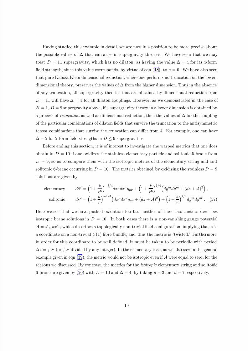
Before ending this section, it is of interest to investigate the warped metrics that one does
obtain in D = 10 if one oxidizes the stainless elementary particle and solitonic 5-brane from
D = 9, so as to compare them with the isotropic metrics of the elementary string and and
solitonic 6-brane occurring in D = 10. The metrics obtained by oxidizing the stainless D = 9
solutions are given by
elementary : ds2 =
1 +kr6−7/4
dxµdxν ηµν +
1 +kr61/4
dymdym + (dz + A)2
,
solitonic : ds2 =
1 +k
r
−1/4dxµdxν ηµν + (dz + A)2
+
1 +k
r
7/4dymdym . (57)
Here we see that we have pushed oxidation too far: neither of these two metrics describes
isotropic brane solutions in D = 10. In both cases there is a non-vanishing gauge potential
A = AM dxM , which describes a topologically non-trivial field configuration, implying that z is
a coordinate on a non-trivial U (1) fibre bundle, and thus the metric is ‘twisted.’ Furthermore,
in order for this coordinate to be well defined, it must be taken to be periodic with period
∆z = F (or F divided by any integer). In the elementary case, as we also saw in the general
example given in eqn (39), the metric would not be isotropic even if A were equal to zero, for the
reasons we discussed. By contrast, the metrics for the isotropic elementary string and solitonic
6-brane are given by (20) with D = 10 and ∆ = 4, by taking d = 2 and d = 7 respectively.
19
8/3/2019 H. Lu et al- Stainless Super p-branes
http://slidepdf.com/reader/full/h-lu-et-al-stainless-super-p-branes 21/35
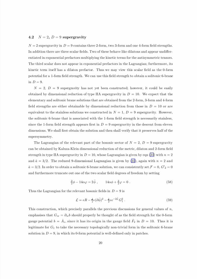
4.2 N = 2, D = 9 supergravity
N = 2 supergravity in D = 9 contains three 2-form, two 3-form and one 4-form field strengths.
In addition there are three scalar fields. Two of these behave like dilatons and appear undiffer-
entiated in exponential prefactors multiplying the kinetic terms for the antisymmetric tensors.
The third scalar does not appear in exponential prefactors in the Lagrangian; furthermore, its
kinetic term itself has a dilaton prefactor. Thus we may view this scalar field as the 0-form
potential for a 1-form field strength. We can use this field strength to obtain a solitonic 6-brane
in D = 9.
N = 2, D = 9 supergravity has not yet been constructed; however, it could be easily
obtained by dimensional reduction of type IIA supergravity in D = 10. We expect that the
elementary and solitonic brane solutions that are obtained from the 2-form, 3-form and 4-form
field strengths are either obtainable by dimensional reduction from those in D = 10 or are
equivalent to the stainless solutions we constructed in N = 1, D = 9 supergravity. However,
the solitonic 6-brane that is associated with the 1-form field strength is necessarily stainless,
since the 1-form field strength appears first in D = 9 supergravity in the descent from eleven
dimensions. We shall first obtain the solution and then shall verify that it preserves half of the
supersymmetry.
The Lagrangian of the relevant part of the bosonic sector of N = 2, D = 9 supergravity
can be obtained by Kaluza-Klein dimensional reduction of the metric, dilaton and 2-form field
strength in type IIA supergravity in D = 10, whose Lagrangian is given by eqn (31) with n = 2
and a = 3/2. The reduced 9-dimensional Lagrangian is given by (35), again with n = 2 and
a = 3/2. In order to obtain a solitonic 6-brane solution, we can consistently set F = 0, G2 = 0
and furthermore truncate out one of the two scalar field degrees of freedom by setting
32φ − 14αϕ = 2φ , 14αφ + 3
2ϕ = 0 . (58)
Thus the Lagrangian for the relevant bosonic fields in D = 9 is
L = eR − 12e(∂ φ)2 − 1
2ee−2φ G21 . (59)
This construction, which precisely parallels the previous discussions for general values of n,
emphasises that GM = ∂ M b should properly be thought of as the field strength for the 0-form
gauge potential b = Az, since it has its origin in the gauge field F 2 in D = 10. Thus it is
legitimate for G1 to take the necessary topologically non-trivial form in the solitonic 6-brane
solution in D = 9, in which its 0-form potential is well-defined only in patches.
20
8/3/2019 H. Lu et al- Stainless Super p-branes
http://slidepdf.com/reader/full/h-lu-et-al-stainless-super-p-branes 22/35
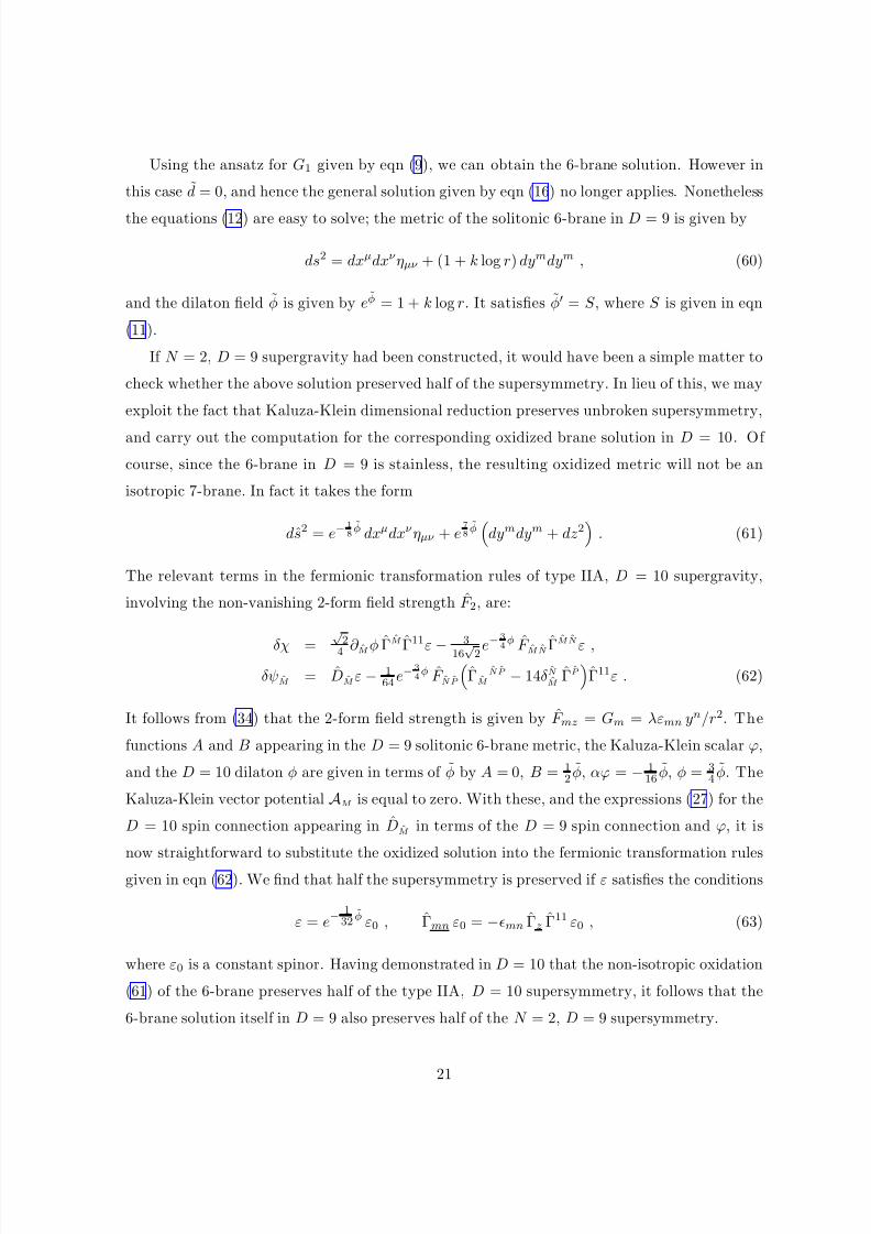
Using the ansatz for G1 given by eqn (9), we can obtain the 6-brane solution. However in
this case d = 0, and hence the general solution given by eqn (16) no longer applies. Nonetheless
the equations (12) are easy to solve; the metric of the solitonic 6-brane in D = 9 is given by
ds2 = dxµdxν ηµν + (1 + k log r) dymdym , (60)
and the dilaton field φ is given by eφ = 1 + k log r. It satisfies φ = S , where S is given in eqn
(11).
If N = 2, D = 9 supergravity had been constructed, it would have been a simple matter to
check whether the above solution preserved half of the supersymmetry. In lieu of this, we may
exploit the fact that Kaluza-Klein dimensional reduction preserves unbroken supersymmetry,
and carry out the computation for the corresponding oxidized brane solution in D = 10. Of
course, since the 6-brane in D = 9 is stainless, the resulting oxidized metric will not be an
isotropic 7-brane. In fact it takes the form
ds2 = e−1
8φ dxµdxν ηµν + e
7
8φ
dymdym + dz2
. (61)
The relevant terms in the fermionic transformation rules of type IIA, D = 10 supergravity,
involving the non-vanishing 2-form field strength F 2, are:
δχ =
√24 ∂ M φ Γ
M
Γ11
ε −3
16√2e−3
4φ
F M N ΓM N
ε ,
δψM = DM ε − 164e−
3
4φ F N P
ΓM
N P − 14δN M
ΓP
Γ11ε . (62)
It follows from (34) that the 2-form field strength is given by F mz = Gm = λεmn yn/r2. The
functions A and B appearing in the D = 9 solitonic 6-brane metric, the Kaluza-Klein scalar ϕ,
and the D = 10 dilaton φ are given in terms of φ by A = 0, B = 12 φ, αϕ = − 1
16 φ, φ = 34 φ. The
Kaluza-Klein vector potential AM is equal to zero. With these, and the expressions (27) for the
D = 10 spin connection appearing in DM in terms of the D = 9 spin connection and ϕ, it is
now straightforward to substitute the oxidized solution into the fermionic transformation rules
given in eqn (62). We find that half the supersymmetry is preserved if ε satisfies the conditions
ε = e−132 φ ε0 , Γmn ε0 = −mn Γz Γ11 ε0 , (63)
where ε0 is a constant spinor. Having demonstrated in D = 10 that the non-isotropic oxidation
(61) of the 6-brane preserves half of the type IIA, D = 10 supersymmetry, it follows that the
6-brane solution itself in D = 9 also preserves half of the N = 2, D = 9 supersymmetry.
21
8/3/2019 H. Lu et al- Stainless Super p-branes
http://slidepdf.com/reader/full/h-lu-et-al-stainless-super-p-branes 23/35
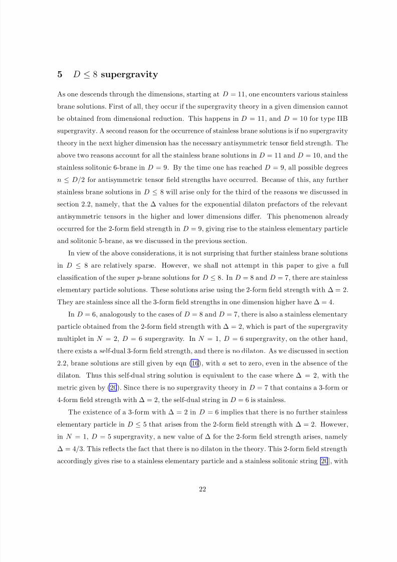
5 D ≤ 8 supergravity
As one descends through the dimensions, starting at D = 11, one encounters various stainless
brane solutions. First of all, they occur if the supergravity theory in a given dimension cannot
be obtained from dimensional reduction. This happens in D = 11, and D = 10 for type IIB
supergravity. A second reason for the occurrence of stainless brane solutions is if no supergravity
theory in the next higher dimension has the necessary antisymmetric tensor field strength. The
above two reasons account for all the stainless brane solutions in D = 11 and D = 10, and the
stainless solitonic 6-brane in D = 9. By the time one has reached D = 9, all possible degrees
n ≤ D/2 for antisymmetric tensor field strengths have occurred. Because of this, any further
stainless brane solutions in D≤
8 will arise only for the third of the reasons we discussed in
section 2.2, namely, that the ∆ values for the exponential dilaton prefactors of the relevant
antisymmetric tensors in the higher and lower dimensions differ. This phenomenon already
occurred for the 2-form field strength in D = 9, giving rise to the stainless elementary particle
and solitonic 5-brane, as we discussed in the previous section.
In view of the above considerations, it is not surprising that further stainless brane solutions
in D ≤ 8 are relatively sparse. However, we shall not attempt in this paper to give a full
classification of the super p-brane solutions for D ≤ 8. In D = 8 and D = 7, there are stainless
elementary particle solutions. These solutions arise using the 2-form field strength with ∆ = 2.
They are stainless since all the 3-form field strengths in one dimension higher have ∆ = 4.
In D = 6, analogously to the cases of D = 8 and D = 7, there is also a stainless elementary
particle obtained from the 2-form field strength with ∆ = 2, which is part of the supergravity
multiplet in N = 2, D = 6 supergravity. In N = 1, D = 6 supergravity, on the other hand,
there exists a self-dual 3-form field strength, and there is no dilaton. As we discussed in section
2.2, brane solutions are still given by eqn (16), with a set to zero, even in the absence of the
dilaton. Thus this self-dual string solution is equivalent to the case where ∆ = 2, with the
metric given by (20). Since there is no supergravity theory in D = 7 that contains a 3-form or
4-form field strength with ∆ = 2, the self-dual string in D = 6 is stainless.
The existence of a 3-form with ∆ = 2 in D = 6 implies that there is no further stainless
elementary particle in D ≤ 5 that arises from the 2-form field strength with ∆ = 2. However,
in N = 1, D = 5 supergravity, a new value of ∆ for the 2-form field strength arises, namely
∆ = 4/3. This reflects the fact that there is no dilaton in the theory. This 2-form field strength
accordingly gives rise to a stainless elementary particle and a stainless solitonic string [20], with
22
8/3/2019 H. Lu et al- Stainless Super p-branes
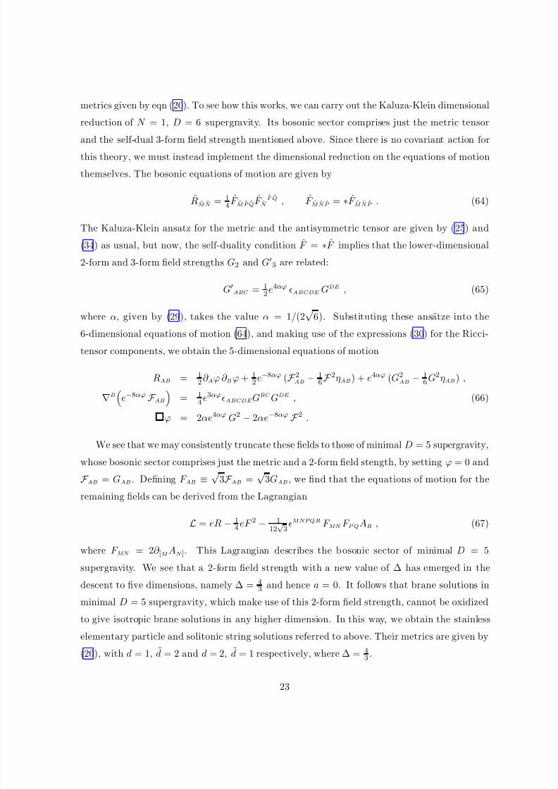
http://slidepdf.com/reader/full/h-lu-et-al-stainless-super-p-branes 24/35
metrics given by eqn (20). To see how this works, we can carry out the Kaluza-Klein dimensional
reduction of N = 1, D = 6 supergravity. Its bosonic sector comprises just the metric tensor
and the self-dual 3-form field strength mentioned above. Since there is no covariant action for
this theory, we must instead implement the dimensional reduction on the equations of motion
themselves. The bosonic equations of motion are given by
RM N = 14 F M P QF N
P Q , F M N P = ∗F M N P . (64)
The Kaluza-Klein ansatz for the metric and the antisymmetric tensor are given by ( 25) and
(34) as usual, but now, the self-duality condition F = ∗F implies that the lower-dimensional
2-form and 3-form field strengths G2 and G3 are related:
GABC = 1
2e4αϕ ABCDE GDE , (65)
where α, given by (29), takes the value α = 1/(2√
6). Substituting these ansatze into the
6-dimensional equations of motion (64), and making use of the expressions (30) for the Ricci-
tensor components, we obtain the 5-dimensional equations of motion
RAB = 12∂ Aϕ ∂ Bϕ + 1
2e−8αϕ (F 2AB
− 16F 2ηAB) + e4αϕ (G2
AB− 1
6G2ηAB) ,
B
e−8αϕ F AB
= 14e3αϕABCDEGBCGDE , (66)
ϕ = 2αe4αϕ G2 − 2αe−8αϕ F 2 .
We see that we may consistently truncate these fields to those of minimal D = 5 supergravity,
whose bosonic sector comprises just the metric and a 2-form field stength, by setting ϕ = 0 and
F AB = GAB. Defining F AB ≡ √3F AB =
√3GAB, we find that the equations of motion for the
remaining fields can be derived from the Lagrangian
L = eR − 14eF 2 − 1
12√3
MNPQR F MN F PQAR , (67)
where F MN = 2∂ [M AN ]. This Lagrangian describes the b osonic sector of minimal D = 5supergravity. We see that a 2-form field strength with a new value of ∆ has emerged in the
descent to five dimensions, namely ∆ = 43 and hence a = 0. It follows that brane solutions in
minimal D = 5 supergravity, which make use of this 2-form field strength, cannot be oxidized
to give isotropic brane solutions in any higher dimension. In this way, we obtain the stainless
elementary particle and solitonic string solutions referred to above. Their metrics are given by
(20), with d = 1, d = 2 and d = 2, d = 1 respectively, where ∆ = 43 .
23
8/3/2019 H. Lu et al- Stainless Super p-branes
http://slidepdf.com/reader/full/h-lu-et-al-stainless-super-p-branes 25/35
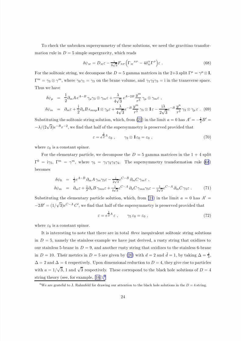
To check the unbroken supersymmetry of these solutions, we need the gravitino transfor-
mation rule in D = 5 simple supergravity, which reads
δψM = DM ε − i8√3
F NP ΓM
NP − 4δN M ΓP ε . (68)
For the solitonic string, we decompose the D = 5 gamma matrices in the 2+3 split Γµ = γ µ⊗1l,
Γm = γ 3 ⊗ γ m, where γ 0γ 1 = γ 3 on the brane volume, and γ 1γ 2γ 3 = i in the transverse space.
Thus we have
δψµ =1
2∂ mA eA−B γ µγ 3 ⊗ γ mε +
λ
4√
3eA−2B ym
r3γ µ ⊗ γ mε ,
δψm = ∂ mε +i
2∂ nB mnp1l ⊗ γ pε +
λ
4√
3e−B
ym
r3γ 3 ⊗ 1l ε − iλ
2√
3e−B
yn
r3γ 3 ⊗ γ p ε . (69)
Substituting the solitonic string solution, which, from (21) in the limit a = 0 has A = −12B =
−λ/(2√
3)e−Br−2, we find that half of the supersymmetry is preserved provided that
ε = e12A ε0 , γ 3 ⊗ 1l ε0 = ε0 , (70)
where ε0 is a constant spinor.
For the elementary particle, we decompose the D = 5 gamma matrices in the 1 + 4 split
Γ0 = iγ 5, Γm = γ m, where γ 5 = γ 1γ 2γ 3γ 4. The supersymmetry transformation rule (68)
becomes
δψ0 = i2eA−B ∂ mA γ mγ 5ε − i2√3eC −B ∂ mC γ mε ,
δψm = ∂ mε + 12∂ nB γ mnε + 1
4√3
eC −A ∂ nC γ mnγ 5ε − 12√3
eC −A ∂ mC γ 5ε . (71)
Substituting the elementary particle solution, which, from (21) in the limit a = 0 has A =
−2B = (1/√
3)eC −A C , we find that half of the supersymmetry is preserved provided that
ε = e12A ε , γ 5 ε0 = ε0 , (72)
where ε0 is a constant spinor.
It is interesting to note that there are in total three inequivalent solitonic string solutions
in D = 5, namely the stainless example we have just derived, a rusty string that oxidizes to
our stainless 5-brane in D = 9, and another rusty string that oxidizes to the stainless 6-brane
in D = 10. Their metrics in D = 5 are given by (20) with d = 2 and d = 1, by taking ∆ = 43 ,
∆ = 2 and ∆ = 4 respectively. Upon dimensional reduction to D = 4, they give rise to particles
with a = 1/√
3, 1 and√
3 respectively. These correspond to the black hole solutions of D = 4
string theory (see, for example, [16]).6
6We are grateful to J. Rahmfeld for drawing our attention to the black hole solutions in the D = 4 string.
24
8/3/2019 H. Lu et al- Stainless Super p-branes
http://slidepdf.com/reader/full/h-lu-et-al-stainless-super-p-branes 26/35
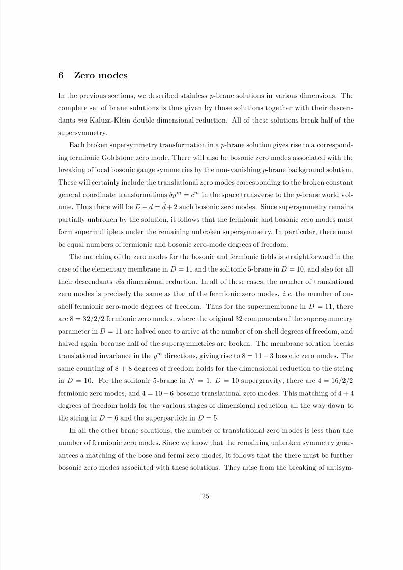
6 Zero modes
In the previous sections, we described stainless p-brane solutions in various dimensions. The
complete set of brane solutions is thus given by those solutions together with their descen-
dants via Kaluza-Klein double dimensional reduction. All of these solutions break half of the
supersymmetry.
Each broken supersymmetry transformation in a p-brane solution gives rise to a correspond-
ing fermionic Goldstone zero mode. There will also be bosonic zero modes associated with the
breaking of local bosonic gauge symmetries by the non-vanishing p-brane background solution.
These will certainly include the translational zero modes corresponding to the broken constant
general coordinate transformations δym = cm in the space transverse to the p-brane world vol-
ume. Thus there will be D − d = d + 2 such bosonic zero modes. Since supersymmetry remains
partially unbroken by the solution, it follows that the fermionic and bosonic zero modes must
form supermultiplets under the remaining unbroken supersymmetry. In particular, there must
be equal numbers of fermionic and bosonic zero-mode degrees of freedom.
The matching of the zero modes for the bosonic and fermionic fields is straightforward in the
case of the elementary membrane in D = 11 and the solitonic 5-brane in D = 10, and also for all
their descendants via dimensional reduction. In all of these cases, the number of translational
zero modes is precisely the same as that of the fermionic zero modes, i.e. the number of on-
shell fermionic zero-mode degrees of freedom. Thus for the supermembrane in D = 11, there
are 8 = 32/2/2 fermionic zero modes, where the original 32 components of the supersymmetry
parameter in D = 11 are halved once to arrive at the number of on-shell degrees of freedom, and
halved again because half of the supersymmetries are broken. The membrane solution breaks
translational invariance in the ym directions, giving rise to 8 = 11 − 3 bosonic zero modes. The
same counting of 8 + 8 degrees of freedom holds for the dimensional reduction to the string
in D = 10. For the solitonic 5-brane in N = 1, D = 10 supergravity, there are 4 = 16/2/2
fermionic zero modes, and 4 = 10
−6 bosonic translational zero modes. This matching of 4 + 4
degrees of freedom holds for the various stages of dimensional reduction all the way down to
the string in D = 6 and the superparticle in D = 5.
In all the other brane solutions, the number of translational zero modes is less than the
number of fermionic zero modes. Since we know that the remaining unbroken symmetry guar-
antees a matching of the bose and fermi zero modes, it follows that the there must be further
bosonic zero modes associated with these solutions. They arise from the breaking of antisym-
25
8/3/2019 H. Lu et al- Stainless Super p-branes
http://slidepdf.com/reader/full/h-lu-et-al-stainless-super-p-branes 27/35
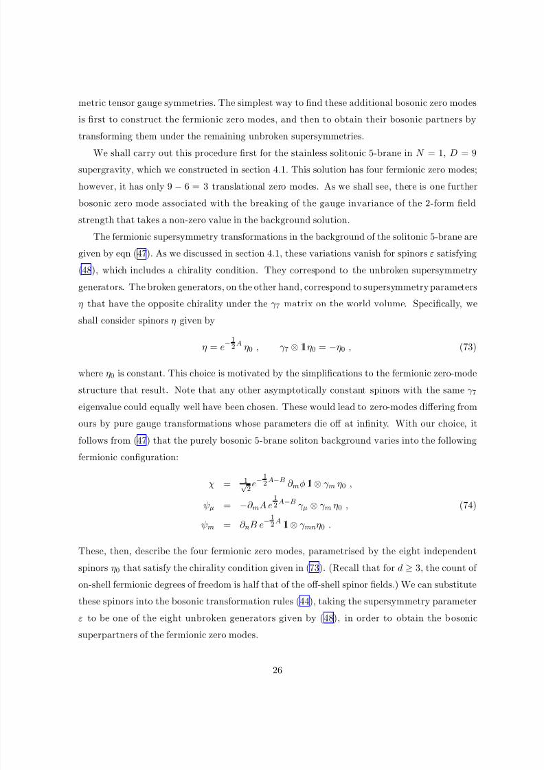
metric tensor gauge symmetries. The simplest way to find these additional bosonic zero modes
is first to construct the fermionic zero modes, and then to obtain their bosonic partners by
transforming them under the remaining unbroken supersymmetries.
We shall carry out this procedure first for the stainless solitonic 5-brane in N = 1, D = 9
supergravity, which we constructed in section 4.1. This solution has four fermionic zero modes;
however, it has only 9 − 6 = 3 translational zero modes. As we shall see, there is one further
bosonic zero mode associated with the breaking of the gauge invariance of the 2-form field
strength that takes a non-zero value in the background solution.
The fermionic supersymmetry transformations in the background of the solitonic 5-brane are
given by eqn (47). As we discussed in section 4.1, these variations vanish for spinors ε satisfying
(48), which includes a chirality condition. They correspond to the unbroken supersymmetry
generators. The broken generators, on the other hand, correspond to supersymmetry parameters
η that have the opposite chirality under the γ 7 matrix on the world volume. Specifically, we
shall consider spinors η given by
η = e−12A η0 , γ 7 ⊗ 1l η0 = −η0 , (73)
where η0 is constant. This choice is motivated by the simplifications to the fermionic zero-mode
structure that result. Note that any other asymptotically constant spinors with the same γ 7
eigenvalue could equally well have been chosen. These would lead to zero-modes differing from
ours by pure gauge transformations whose parameters die off at infinity. With our choice, it
follows from (47) that the purely bosonic 5-brane soliton background varies into the following
fermionic configuration:
χ = 1√2
e−12A−B ∂ mφ 1l ⊗ γ m η0 ,
ψµ = −∂ mA e12A−B γ µ ⊗ γ m η0 , (74)
ψm = ∂ nB e−12A 1l ⊗ γ mnη0 .
These, then, describe the four fermionic zero modes, parametrised by the eight independent
spinors η0 that satisfy the chirality condition given in (73). (Recall that for d ≥ 3, the count of
on-shell fermionic degrees of freedom is half that of the off-shell spinor fields.) We can substitute
these spinors into the bosonic transformation rules (44), taking the supersymmetry parameter
ε to be one of the eight unbroken generators given by (48), in order to obtain the b osonic
superpartners of the fermionic zero modes.
26
8/3/2019 H. Lu et al- Stainless Super p-branes
http://slidepdf.com/reader/full/h-lu-et-al-stainless-super-p-branes 28/35
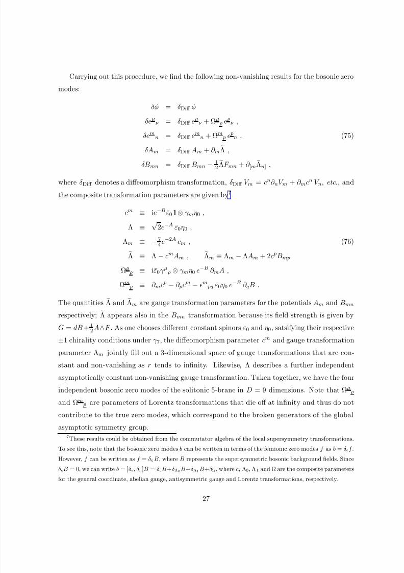
Carrying out this procedure, we find the following non-vanishing results for the bosonic zero
modes:
δφ = δDiff φ
δeµν = δDiff eµν + Ωµ
ρ eρν ,
δemn = δDiff emn + Ωm
p e pn , (75)
δAm = δDiff Am + ∂ mΛ ,
δBmn = δDiff Bmn − 12ΛF mn + ∂ [mΛn] ,
where δDiff denotes a diffeomorphism transformation, δDiff V m = cn∂ nV m + ∂ mcn V n, etc., and
the composite transformation parameters are given by7
cm ≡ ie−B ε01l ⊗ γ mη0 ,
Λ ≡√
2e−A ε0η0 ,
Λm ≡ − 74e−2A cm , (76)
Λ ≡ Λ − cmAm , Λm ≡ Λm − ΛAm + 2c pBmp
Ωµρ ≡ iε0γ µρ ⊗ γ mη0 e−B ∂ mA ,
Ωm p ≡ ∂ mc p − ∂ pcm − m pq ε0η0 e−B ∂ qB .
The quantities Λ and Λm are gauge transformation parameters for the potentials Am and Bmn
respectively; Λ appears also in the Bmn transformation because its field strength is given by
G = dB + 12A∧F . As one chooses different constant spinors ε0 and η0, satsifying their respective
±1 chirality conditions under γ 7, the diffeomorphism parameter cm and gauge transformation
parameter Λm jointly fill out a 3-dimensional space of gauge transformations that are con-
stant and non-vanishing as r tends to infinity. Likewise, Λ describes a further independent
asymptotically constant non-vanishing gauge transformation. Taken together, we have the four
independent bosonic zero modes of the solitonic 5-brane in D = 9 dimensions. Note that Ωµρ
and Ωm p are parameters of Lorentz transformations that die off at infinity and thus do not
contribute to the true zero modes, which correspond to the broken generators of the global
asymptotic symmetry group.7These results could be obtained from the commutator algebra of the local supersymmetry transformations.
To see this, note that the b osonic zero modes b can be written in terms of the femionic zero modes f as b = δf .
However, f can be written as f = δηB, where B represents the supersymmetric bosonic background fields. Since
δB = 0, we can write b = [δ, δη]B = δcB+δΛ0B+δΛ1B+δΩ, where c, Λ0, Λ1 and Ω are the composite parameters
for the general coordinate, abelian gauge, antisymmetric gauge and Lorentz transformations, respectively.
27
8/3/2019 H. Lu et al- Stainless Super p-branes
http://slidepdf.com/reader/full/h-lu-et-al-stainless-super-p-branes 29/35
8/3/2019 H. Lu et al- Stainless Super p-branes
http://slidepdf.com/reader/full/h-lu-et-al-stainless-super-p-branes 30/35
7 Discussion
In this paper, we have searched for supersymmetric p-brane solutions of supergravity theories
in diverse dimensions. As these solutions occur in families related by dimensional reduction,
we have concentrated on the maximal, or stainless, solution in each family. In addition to the
previously-known examples, we have found a number of new solutions in 5 ≤ D ≤ 9 dimensions.
(The lower dimensional bound arises here because we have restricted our attention to solutions of
supergravity theories, and have not considered p-branes in theories with rigid supersymmetry.)
Our new stainless solutions cannot oxidize isotropically to brane solutions in higher dimensions.
Put another way, this means that these new solutions cannot simply be viewed as dimensional
reductions of previously-known brane solutions in D = 11 or D = 10 dimensions.
A question that we have not addressed so far concerns the world brane actions that should
describe the zero-mode fluctuations around the static, isotropic solutions considered here. From
supersymmetry, one has detailed knowledge of the supermultiplet structure of the zero modes
that would appear in a gauge-fixed world brane action. In general, one expects that such gauge-
fixed actions should be extendable to spacetime supersymmetric and Lorentz invariant actions
by adding the appropriate additional unphysical degrees of freedom and their associated local
world volume gauge symmetries. For the four classic sequences of super p-branes, these actions
are generalisations of the D = 10 superstring [17, 1] or D = 11 supermembrane [2] actions.
Very little is known about the structure of the covariant world volume actions for any of the
other p-brane cases; this subject remains an important open problem.
In the absence of detailed knowledge of the world volume action, some information can
be extracted if one assumes that the bosonic sector of the action takes the general form of a
Nambu-Goto action coupled to the spacetime metric, dilaton, and a d-form gauge potential,
with the non-polynomiality removed by the introduction of a world-volume metric γ ij as an
auxiliary field [18]:
I brane = dd
ξ−12√−γγ
ij
∂ iX M
∂ jX N
gMN ebφ
+d
−2
2 √−γ
− 1
d!i1···id ∂ i1X M 1 · · · ∂ idX M d AM 1···M d
. (77)
The exponent b of the dilaton coupling in the first term is a priori unknown. One way of
selecting a value for it in a number of cases is by resorting to an argument based on a scaling
symmetry of the pure supergravity theory [16]. Under the constant rescalings
eφ −→ λα eφ , gMN −→ λ2β gMN , AM 1···M d −→ λγ AM 1···M d , (78)
29
8/3/2019 H. Lu et al- Stainless Super p-branes
http://slidepdf.com/reader/full/h-lu-et-al-stainless-super-p-branes 31/35
the action given by (1) scales by an overall factor λβ (D−2), provided that we choose γ = βd +aα.
Requiring that I brane scale in the same way, one finds that the parameters must be related by
α =dd
a(D − 2), β =
d
D − 2γ = d , b =
a
d. (79)
Substituting the ansatze (4) and (7) into (77), one finds that the branewave equation following
from (77) implies [16]
(eC ) = (edA+aφ/2) . (80)
Comparing with the solution given by (16) and (17), one finds that a must satisfy
a2 = 4 − 2dd
D − 2. (81)
Thus requiring that the elementary brane solution should also satisfy the branewave equation,
with the parameter b in (77) determined by requiring the above scaling symmetry, the value of
a appearing in (1) is in all cases given by (18) with ∆ = 4.
All of the antisymmetric tensors in D = 11 and D = 10 supergravities have ∆ = 4, as
we have seen. Thus the elementary p-brane solutions associated to these antisymmetric tensors
accord with the above discussion. However, as we have seen, there are other values of ∆ that also
occur in lower dimensional supergravity theories. Elementary p-brane solutions in such cases
cannot have zero modes that are described by the action (77) with the choice of parameter b
dictated by the scaling symmetry. An example is provided by the self-dual string in D = 6,
for which the self-dual 3-form has ∆ = 2. In this case, since there is no action for N = 1,
D = 6 supergravity, one has to implement the scaling argument at the level of the equations of
motion. The supergravity equations of motion themselves (64) are invariant under the scaling
gMN −→ λ2β gMN and GMNP −→ λ2β GMNP , for arbitrary β . However, the energy-momentum
tensor T MN (x) = − d2ξ
√−γγ ij∂ iX P ∂ jX Q gMP gNQδ6(x − X )/√−g scales with a factor λ−2β .
Thus the coupled supergravity-string equations break the scaling symmetry. In fact all of the
new stainless elementary p-branes, which have ∆ = 2 or ∆ = 43 , exhibit a similar breaking of
the scaling symmetry in their couplings.
The ultimate significance of the scaling symmetry used in the above arguments remains
unclear to us. Are elementary p-brane solutions that respect the scaling symmetry in their cou-
plings more fundamental than others? We do not have an answer to this question at present.
We would remark, however, that couplings that break scaling symmetries present in pure un-
coupled gravity and supergravity theories are not at all uncommon. Take, for example, a
massless charged particle coupled to Einstein-Maxwell theory in D = 4. The Einstein-Maxwell
30
8/3/2019 H. Lu et al- Stainless Super p-branes
http://slidepdf.com/reader/full/h-lu-et-al-stainless-super-p-branes 32/35
action I =
d4x(eR − 14eF 2) in the absence of the particle coupling scales as I −→ ρ2I under
gµν −→ ρ2gµν , Aµ −→ ρAµ. But once the particle is coupled in, via the standard worldline-
reparametrisation invariant action dτ (e−1X µX ν gµν + AµX µ), the scaling symmetry is broken
by the electromagnetic coupling AµX µ.
Another reason why the status of the scaling symmetries remains in doubt comes from quan-
tisation. The supergravity theories arising as low-energy effective field theories of superstring
theories have field equations determined via the beta functions from the requirement that the
string’s conformal invariance be preserved. The leading terms of these effective field equations
reproduce standard supergravity field equations, but there are also an infinite series of quantum
corrections, all of which break the scaling symmetries.
Nonetheless, it is intriguing that a purely bosonic discussion based upon the coupling of
Nambu-Goto-type actions and preservation of scaling symmetries fixes dilaton couplings to
antisymmetric tensor gauge fields in a way that agrees with many of the couplings actually
found in supergravity theories (i.e. the ∆ = 4 couplings).
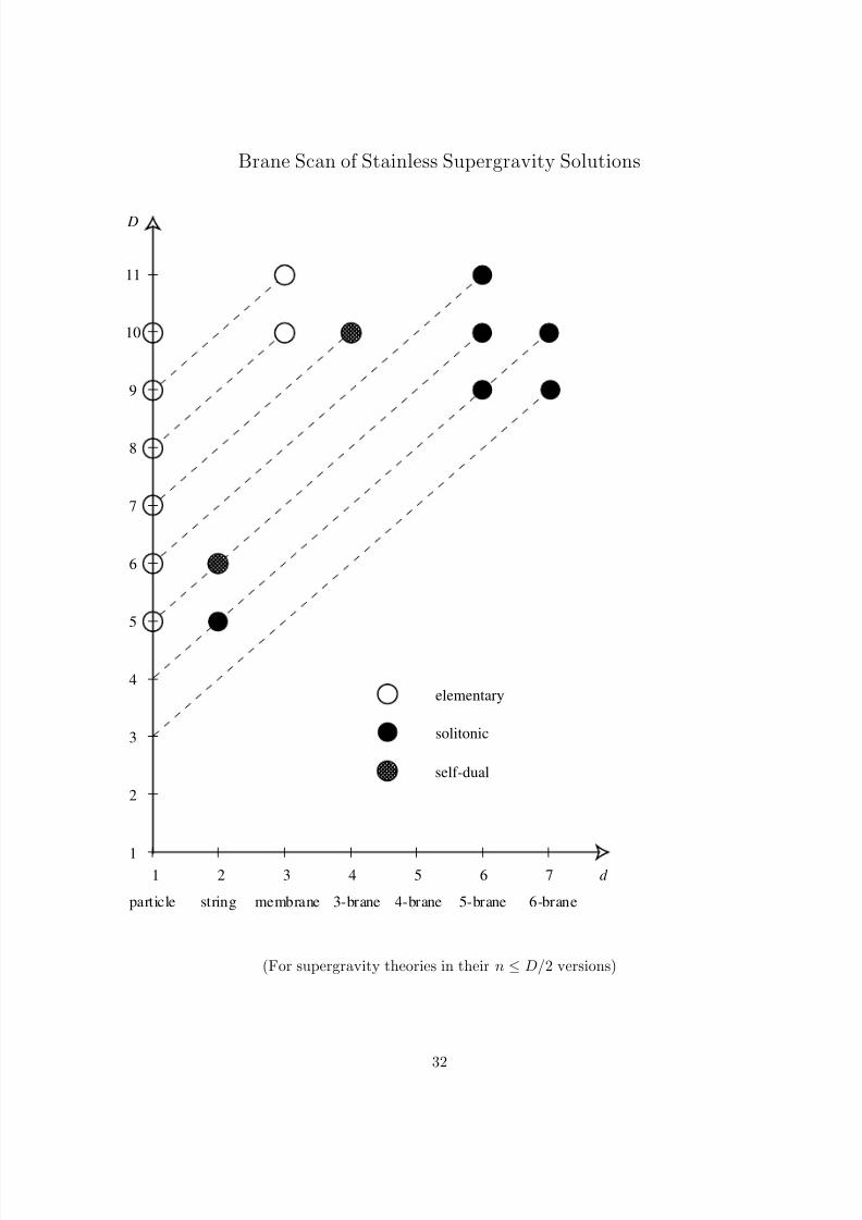
In concluding, we shall summarise the results that we have obtained in this paper in a revised
brane-scan, in which we plot only the stainless members of each p-brane family. In accordance
with our discussion at the end of section 2.1, we may, without loss of generality, consider
only the versions of the various supergravity theories where all the antisymmetric tensors have
degrees n ≤ D/2, since no further inequivalent elementary or solitonic brane solutions arise fromdualised versions of the theories. Accordingly, in the stainless brane-scan, we denote solutions
of the n ≤ D/2 theories that are elementary by open circles, solutions that are solitonic by solid
circles, and self-dual solutions by cross-hatched circles. The dashed lines extending diagonally
downwards from the various points on the brane scan indicate that each stainless solution gives
rise to its own set of dimensionally-reduced descendants.
31
8/3/2019 H. Lu et al- Stainless Super p-branes
http://slidepdf.com/reader/full/h-lu-et-al-stainless-super-p-branes 33/35
Brane Scan of Stainless Supergravity Solutions
1
2
3
4
5
6
7
8
9
10
11
1 2 3 4 5 6 7
particle string membrane 3-brane 4-brane 5-brane 6-brane
d
D
elementary
solitonic
self-dual
(For supergravity theories in their n ≤ D/2 versions)
32
8/3/2019 H. Lu et al- Stainless Super p-branes
http://slidepdf.com/reader/full/h-lu-et-al-stainless-super-p-branes 34/35
Acknowledgements
H.L., C.N.P. and K.S.S. thank SISSA, Trieste, and E.S. thanks ICTP, Trieste, for hospitality
during the course of this work.
References
[1] J. Hughes, J. Liu and J. Polchinski, Phys. Lett. B180 (1986) 370.
[2] E. Bergshoeff, E. Sezgin and P.K. Townsend, Phys. Lett. B189 (1987) 75.
[3] P.K. Townsend, Phys. Lett. B202 (1988) 53.
[4] A. Achucarro, J. Evans, P.K. Townsend and D. Wiltshire, Phys. Lett. B198 (1987) 441.
[5] M.J. Duff, P.S. Howe, T. Inami and K.S. Stelle, Phys. Lett. B191 (1987) 70.
[6] A. Dabholkar, G. W. Gibbons, J. A. Harvey and F. Ruiz Ruiz, Nucl. Phys. B340 (1990)
33.
[7] M.J. Duff and K.S. Stelle, Phys. Lett. B253 (1991) 113.
[8] C.G. Callan and R.R. Khuri, Phys. Lett. B261 (1991) 363; R.R. Khuri, Phys. Lett. 307
(1993) 302; R.R. Khuri, Nucl. Phys. B403 (1993) 335; M.J. Duff and J.X. Lu, Nucl. Phys.
B354 (1991) 141.
[9] C.G. Callan, J.A. Harvey and A. Strominger, Nucl. Phys. B359 (1991) 611; Nucl. Phys.
B367 (1991) 60; Supersymmetric String Solitons, Lectures given at the Trieste Summer
School, Trieste, Italy, 1991; M.J. Duff, R.R. Khuri and J.X. Lu, Nucl. Phys. B377 (1992)
281.
[10] A. Strominger, Nucl. Phys. B343 (1990) 167; M.J. Duff and J.X. Lu, Phys. Rev. Lett. 66
(1991) 1402.
[11] R. Guven, Phys. Lett. B276 (1992) 49; Phys. Lett. B212 (1988) 277.
[12] M.J. Duff and J.X. Lu, Phys. Lett. B273 (1991) 409.
[13] S.J. Gates, H. Nishino and E. Sezgin, Class. Quantum Grav. 3 (1986) 21.
[14] C.N. Pope and K.S. Stelle, Phys. Lett. B198 (1987) 151.
33
8/3/2019 H. Lu et al- Stainless Super p-branes
http://slidepdf.com/reader/full/h-lu-et-al-stainless-super-p-branes 35/35
[15] P.K. Townsend, The eleven-dimensional supermembrane revisited , hep-th/9501068.
[16] M.J. Duff, R.R. Khuri and J.X. Lu, String solitons, hep-th/9412184.
[17] M.B. Green and J.H. Schwarz, Phys. Lett. B136 (1984) 367.
[18] L. Brink, P.S. Howe and P. Di Vecchia, Phys. Lett. B65 (1976) 471.
[19] M.J. Duff and J.X. Lu, Nucl. Phys. B416 (1994) 301.
[20] G.W. Gibbons, G. Horowitz and P.K. Townsend, Class. Quant. Grav. 12 (1995) 297; G.W.
Gibbons, D. Kastor, L.A.J. London, P.K. Townsend and J. Traschen, Nucl. Phys. 416
(1994) 850.
[21] A. Salam and E. Sezgin, Supergravities in Diverse Dimensions, Vols. 1 & 2, World Scientific,
1989.